Embed Size (px)
Citation preview
Thermo-Calc Graphical Mode User Guide
Version 3.1
© 1995-2013 Foundation of Computational Thermodynamics
Stockholm, Sweden
Thermo-Calc Graphical User Guide Version 3.1
1
Thermo-Calc Graphical Mode User Guide
Contents 1 Introduction ........................................................................................................................ 3
1.1 The Thermo-Calc program ............................................................................ 3
1.2 Documentation for Thermo-Calc Graphical Mode ............................... 3
1.2.1 This User Guide ............................................................................... 3
1.2.2 Using online help ............................................................................ 4
1.2.3 The Thermo-Calc Graphical Examples .................................... 4
1.3 Program overview ............................................................................................ 5
1.3.1 Activity types .................................................................................... 5
2 Using the graphical interface ....................................................................................... 6
2.1 The Thermo-Calc Graphical mode interface .......................................... 6
2.2 Using the graphical mode interface ........................................................... 7
2.3 Default options ................................................................................................... 8
2.4 Workflow .............................................................................................................. 9
3 Using the Quick Start wizard .................................................................................... 10
3.1 How to use the Quick Start wizard ......................................................... 10
4 Working with Thermo-Calc projects ..................................................................... 11
4.1 Using templates .............................................................................................. 12
4.2 Creating activities and successors .......................................................... 13
4.2.1 Cloning activities and trees ..................................................... 13
4.2.2 Manipulating your activity tree and using the grid ....... 15
4.3 Performing projects, trees and activities ............................................. 16
4.3.1 Status markers in the “Project” window ............................ 17
4.3.2 Using the Scheduler .................................................................... 18
4.3.3 Status markers in the “Scheduler” window ...................... 18
4.3.4 Managing the schedule .............................................................. 19
4.3.5 The Event Log ............................................................................... 19
4.4 Using Thermo-Calc project files ............................................................... 20
5 The activities ................................................................................................................... 20
5.1 System definer ................................................................................................. 20
5.1.1 Predecessors and successors ................................................. 20
5.1.2 How to select a database and define your elements ..... 20
5.1.3 How to append data from an additional database ......... 21
5.2 Equilibrium Calculator ................................................................................. 22
5.2.1 Predecessors and successors ................................................. 22
5.2.2 Setting conditions for different calculations .................... 22
5.2.3 Setting conditions – advanced mode ................................... 24
5.2.4 How to calculate with a fixed phase .................................... 24
Thermo-Calc Graphical User Guide Version 3.1
2
5.2.5 How to calculate and plot your own functions ................ 25
5.3 Plot renderer .................................................................................................... 27
5.3.1 Predecessors and successors ................................................. 28
5.3.2 Configuration window settings ............................................. 28
5.3.3 Changing the appearance of a plotted diagram .............. 30
5.3.4 Adding labels ................................................................................. 30
5.3.5 Saving your diagram .................................................................. 31
5.3.6 How to plot several calculations in one diagram ........... 31
5.4 Table renderer................................................................................................. 33
5.4.1 Predecessors and successors ................................................. 33
5.4.2 Tabulated results from an equilibrium calculation ....... 33
5.4.3 Tabulated results from a stepping operation .................. 34
5.4.4 Setting number format and number of decimal digits . 35
5.4.5 Setting background colours .................................................... 35
5.4.6 Saving tabulated data ................................................................ 35
5.5 Experimental file reader ............................................................................. 36
5.5.1 Predecessors and successors ................................................. 36
5.5.2 How to plot an experimental data file................................. 36
5.6 Binary calculator ............................................................................................ 36
5.6.1 Predecessors and successors ................................................. 36
5.6.2 Configuration window settings ............................................. 37
5.7 Ternary calculator ......................................................................................... 38
5.7.1 Predecessors and successors ................................................. 38
5.7.2 Configuration window settings ............................................. 39
5.8 Scheil Calculator ............................................................................................. 40
5.8.1 Predecessors and successors ................................................. 40
5.8.2 Configuration window settings ............................................. 40
Thermo-Calc Graphical User Guide Version 3.1
3
1 Introduction
1.1 The Thermo-Calc program
Thermo-Calc is a sophisticated software, database and programming-interface package for performing thermodynamic calculations. It allows you to calculate complex homogeneous and heterogeneous phase equilibria, and plot the results as property diagrams and phase diagrams.
The program fully supports stoichiometric and non-ideal solution models and databases. These models and databases can be used to make calculations on a large variety of materials such as steels, alloys, slags, salts, ceramics, solders, polymers, subcritical aqueous solutions, supercritical electrolyte solutions, non-ideal gases and hydrothermal fluids or organic substances. The calculations can take into account a wide ranges of temperature, pressure and compositions conditions (you can set temperature up to 6000 K and pressure up to 1 Mbar).
There are two interfaces to the Thermo-Calc program, the Console Mode which uses a command line interface and the Graphical Mode which has a graphical user interface (GUI). This User Guide describes the use of the Thermo-Calc program in the Graphical Mode.
1.2 Documentation for Thermo-Calc Graphical Mode
Apart from this document, you can use the following documentation to learn more about how to use Thermo-Calc in the Graphical mode:
Online help in the Thermo-Calc Graphical mode contains general information about the Graphical mode, information about most “Configuration” window settings, as well as descriptions of two step-by-step examples.
Thermo-Calc Graphical Examples Collection contains eight example Thermo-Calc project files (*.TCU) that demonstrate a few ways in which you can use Thermo-Calc in the Graphical mode.
TC 3.1 Examples
contains brief descriptions of all the examples in the Thermo-Calc Graphical Examples Collection.
Additional documentation and educational materials are also available on Thermo-Calc Software’s website.
1.2.1 This User Guide
Target group
This user guide is intended for new users of the Thermo-Calc Graphical mode that are not familiar with its interface. It is expected, however, that such a user does understand the basics of thermodynamics.
Thermo-Calc Graphical User Guide Version 3.1
4
Purpose
This Thermo-Calc Graphical User Guide is intended to get you started using Thermo-Calc in the Graphical mode. It gives you a brief overview of the program and its underlying structure, describes the GUI, and describes how you define your system of components, set up calculations, run them and visualize the results.
Content
The following conventions will be used:
Buttons that you can click on in the GUI will be enclosed with “«” and “»”, the “much smaller than” and “much greater than” symbols. For example, «Create New Activity».
Menu items, window titles and field names are enclosed in quotation marks. For example, “Composition Unit”.
The vertical line (“|”) indicates menu structure. For example, “select Tools | Options” means that you should select the menu item “Options” from the “Tools” menu.
1.2.2 Using online help
You can access online help information in several ways:
Select Help | Help Contents to open a list of online help contents in your default web browser. Click “Graphical Mode” to get access to all the help pages that are available in the GUI.
In one of the main windows of the Graphical Mode GUI, the “Configuration” window, you can click the help button to view help information regarding the tab that is currently shown in this window. The help information will be shown in your default web browser. The help button looks like this:
1.2.3 The Thermo-Calc Graphical Examples
To learn more about how to use Thermo-Calc, you can open and run the example projects in the Thermo-Calc Graphical Examples Collection. These are in the format of Thermo-Calc project files (*.TCU).
The examples are the following:
1 Calculating a single-point equilibrium
2 Stepping in temperature in the Fe-C system
3 The Fe-C phase diagram
4 Ternary phase diagram in the Fe-Cr-C system at 1000 K
5 The stable and the metastable Fe-C phase diagrams
6 Serially coupled equilibrium calculators
7 User defined functions
8 Scheil and equilibrium solidification
Thermo-Calc Graphical User Guide Version 3.1
5
1.3 Program overview
The Thermo-Calc software architecture consists of modules that handle, for example, database retrieval and management, calculation, visualization and diagram plotting. See the Thermo-Calc Console Mode User Guide for more information about the modular architecture of the software.
Most of the calculation types that can be performed in the Console mode can also be performed in Graphical mode. However, you can only do data optimization and thermodynamic or kinetic assessments in the Console mode.
The two modes can be run simultaneously, but there is no communication between them. What you do in the Graphical mode will not affect the state of the Console mode session and vice versa. There is one exception to this. The options you set for plotting in the “Results” window or the “Console Results” window are applied to how diagrams are plotted in both modes.
In the Thermo-Calc Graphical mode, calculations are always set up, carried out, and visualized as part of a project. These different steps in your project is performed by different types of activities.
1.3.1 Activity types
The following table gives a brief description of each of the seven available activity types:
Activity type Description System Definer The System Definer activity is used
to define a certain thermodynamic system and to read it from file into memory.
(Appended System) To read data from multiple databases, multiple System Definer activities must be created and linked serially. The successor System Definer activities thus defined will by default be named Appended System.
Equilibrium Calculator The Equilibrium Calculator activity is used to set thermodynamic conditions and to define axis variables when a series of equilibrium calculations are to be performed in one or more dimensions.
Plot Renderer The Plot Renderer activity is used to determine the layout of non-text based output.
Table Renderer A table renderer activity is used for text based output.
Binary Calculator The Binary Calculator activity can be used for some calculations involving two components only. It can be thought of as a combination
Thermo-Calc Graphical User Guide Version 3.1
6
of a System Definer activity and an Equilibrium Calculator activity with certain adaptations to simplify the configuration of calculations on binary systems. Note that, to perform this activity successfully, you need a database that was designed for the Binary Calculator, such as the TCBIN database for example.
Ternary Calculator The Ternary Calculator activity can be used for some calculations involving three components. It can be thought of as a combination of a System Definer activity and an Equilibrium Calculator activity with certain adaptations to simplify the configuration of calculations on ternary systems. Note that, to get a reliable result from performing this activity, you need a database that contains fully assessed binary and ternary systems.
Scheil Calculator The Scheil Calculator activity is used to perform Scheil-Gulliver calculations (also known as Scheil calculations). A default Scheil calculation is used to estimate the solidification range of an alloy assuming that i) the liquid phase is homogeneous at all times and ii) the diffusivity is zero in the solid. However, it is possible to disregard the second assumption for selected components.
2 Using the graphical interface
This section introduces you to the GUI and describes the basic workflow of the program.
2.1 The Thermo-Calc Graphical mode interface
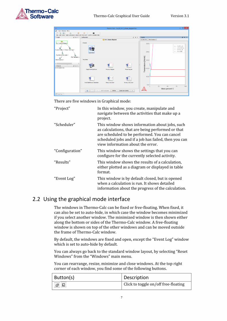
The GUI consist of four types of windows and a toolbar. The following screen shot shows the GUI with the standard window layout.
Thermo-Calc Graphical User Guide Version 3.1
7
There are five windows in Graphical mode:
“Project” In this window, you create, manipulate and navigate between the activities that make up a project.
“Scheduler” This window shows information about jobs, such as calculations, that are being performed or that are scheduled to be performed. You can cancel scheduled jobs and if a job has failed, then you can view information about the error.
“Configuration” This window shows the settings that you can configure for the currently selected activity.
“Results” This window shows the results of a calculation, either plotted as a diagram or displayed in table format.
“Event Log” This window is by default closed, but is opened when a calculation is run. It shows detailed information about the progress of the calculation.
2.2 Using the graphical mode interface
The windows in Thermo-Calc can be fixed or free-floating. When fixed, it can also be set to auto-hide, in which case the window becomes minimized if you select another window. The minimized window is then shown either along the bottom or sides of the Thermo-Calc window. A free-floating window is shown on top of the other windows and can be moved outside the frame of Thermo-Calc window.
By default, the windows are fixed and open, except the “Event Log” window which is set to auto-hide by default.
You can always go back to the standard window layout, by selecting “Reset Windows” from the “Windows” main menu.
You can rearrange, resize, minimize and close windows. At the top right corner of each window, you find some of the following buttons.
Button(s) Description
Click to toggle on/off free-floating
Thermo-Calc Graphical User Guide Version 3.1
8
Click to toggle on/off auto-hide.
Click to minimize an open window that has auto-hide turned on. Note that the window will automatically be minimized if you select another window.
Click to close the window. You can open the window again from the “Window” main menu.
2.3 Default options
You can set general settings for Thermo-Calc Graphical mode, as well as default settings for any new activities that will be created, in the “Options” window. To open this window, select “Options” from the “Tools” main menu. The tabs and panes that are relevant for Thermo-Calc Graphical mode are briefly described in the table that follows:
Tab / pane Description General Here you can select whether to turn
on tooltips information. If “Tooltips enabled” is selected, then a small text box will appear when you hold the cursor still above some buttons or other items.
Here you can also select which language that will be used in the program, and change the appearance of the program (“Look and feel”).
In the “Database directory” field, specify in which directory the Thermo-Calc database directory called “data” can be found. Note that you are not supposed to specify the path to where the database files can be found (that is, in the “data” directory), but the path to the directory that contains the “data” directory.
Adjust the “Log Level” slide bar to get more or less information presented in the “Event Log” window.
Default units Here you can specify which unit that will be used as the default for temperature, pressure, amount, composition, energy, volume, and density.
Graphical Mode>
Activities>Calculation
Here you can change the default settings for the Equilibrium
Thermo-Calc Graphical User Guide Version 3.1
9
Calculator. These settings can also be changed locally in each Equilibrium Calculator for that particular activity (in the “Options” tab in the “Configuration” window).
Graphical Mode>
Activities>Plotting
Here you can change the default settings for any diagrams that will be plotted. Note that these settings are shared with the Console Mode. Any changes you make here will also apply to the default settings on the Console Mode>Plotting tab in the “Options” window (and vice versa).
You can also change the settings for plotting locally for a certain Plot Renderer tab in the Console Results window, by right-clicking on a plot and selecting “Properties” from the pop-up menu.
In addition, the colour, stroke (solid/dashed/dotted/dash_dot) and line width of a particular series of lines in a plot can be changed by clicking one of the lines in that series.
Graphical Mode>
Activities>Tabulation
Here you can change the default setting for the Table Renderer activity.
2.4 Workflow
You can set up a whole tree in the Project window and then perform all the activities at once, or create and perform one activity at a time.
The typical workflow is the following:
1 Define your system: Create a System Definer activity, which allows you to select a database and select which elements to have as components in your system. The database and elements are selected in the “Configuration” window.
2 Set up and run your calculation: Create an Equilibrium Calculator activity, which allows you to set the conditions for your calculation (temperature, pressure, etc.) and set axis variables if you want to make a property or phase diagram. The settings of activities are specified in the “Configuration” window.
3 Visualize the results: Create either a Plot Renderer or a Table Renderer activity that present the results of your calculation in diagram or table format. The results are shown in a “Plot Renderer” or a “Table Renderer” tab in the “Results” window. Note that if you do not visualize the results by performing a Plot Renderer or a Table Renderer, then you will not see any calculation results at all, even if you have performed an Equilibrium Calculator.
Thermo-Calc Graphical User Guide Version 3.1
10
3 Using the Quick Start wizard
The “Quick Start” wizard allows you to quickly get started using Thermo-Calc in the Graphical mode, even before you have any knowledge about how to work with Thermo-Calc projects. You can quickly set up, calculate and visualize any of the following:
Single-point equilibrium
Property diagram
Phase diagram
Scheil solidification simulation
3.1 How to use the Quick Start wizard
This section describes how to calculate an equilibrium, a property diagram, a phase diagram, or a Scheil solidification simulation using the Quick start wizard.
Pre-requisites
None.
Procedure
To set up, perform and visualize a calculation using the Quick Start wizard, follow these steps:
Step Action
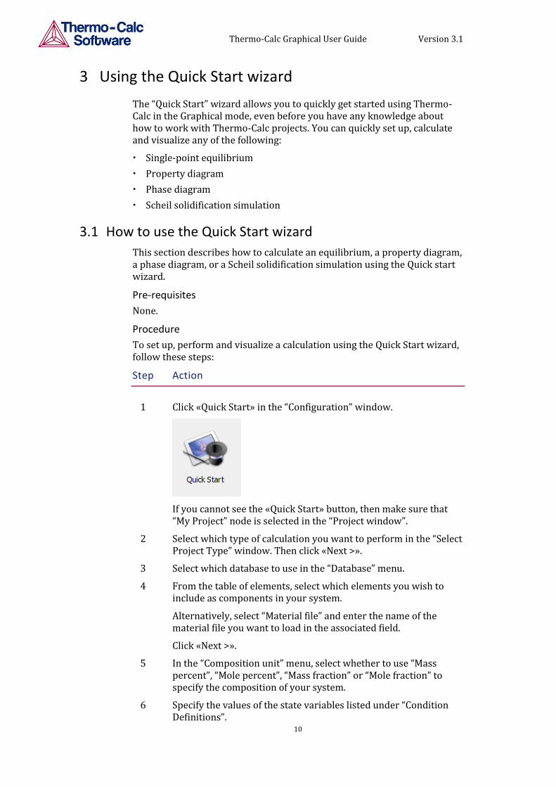
1 Click «Quick Start» in the “Configuration” window.
If you cannot see the «Quick Start» button, then make sure that “My Project” node is selected in the “Project window”.
2 Select which type of calculation you want to perform in the “Select Project Type” window. Then click «Next >».
3 Select which database to use in the “Database” menu.
4 From the table of elements, select which elements you wish to include as components in your system.
Alternatively, select “Material file” and enter the name of the material file you want to load in the associated field.
Click «Next >».
5 In the “Composition unit” menu, select whether to use “Mass percent”, “Mole percent”, “Mass fraction” or “Mole fraction” to specify the composition of your system.
6 Specify the values of the state variables listed under “Condition Definitions”.
Thermo-Calc Graphical User Guide Version 3.1
11
7 If you are calculating a property or a phase diagram, you must also specify the axis variable(s) of the stepping or mapping operation, as well as minimum and maximum values for the variable(s).
If you are calculating a Scheil solidification simulation, then you must select whether you want to account for back-diffusion of any fast-diffusing elements. For those (if any) elements, select “Fast diffuser”.
8 Click «Finish».
The “Event Log” window will now open and show information about the progress of the calculation.
Finally, the diagram is plotted in a “Plot Renderer” tab in the “Results” window. If you have calculated a single-point equilibrium, then a “Table Renderer” tab will show information about the equilibrium.
To save the project, click «Save» on the main toolbar. To save the diagram or table, right-click on the diagram or table and select “Save As” from the pop-up menu.
4 Working with Thermo-Calc projects
This section describes how you create and perform activities for your project, as well as how you manipulate and link various activities in your project.
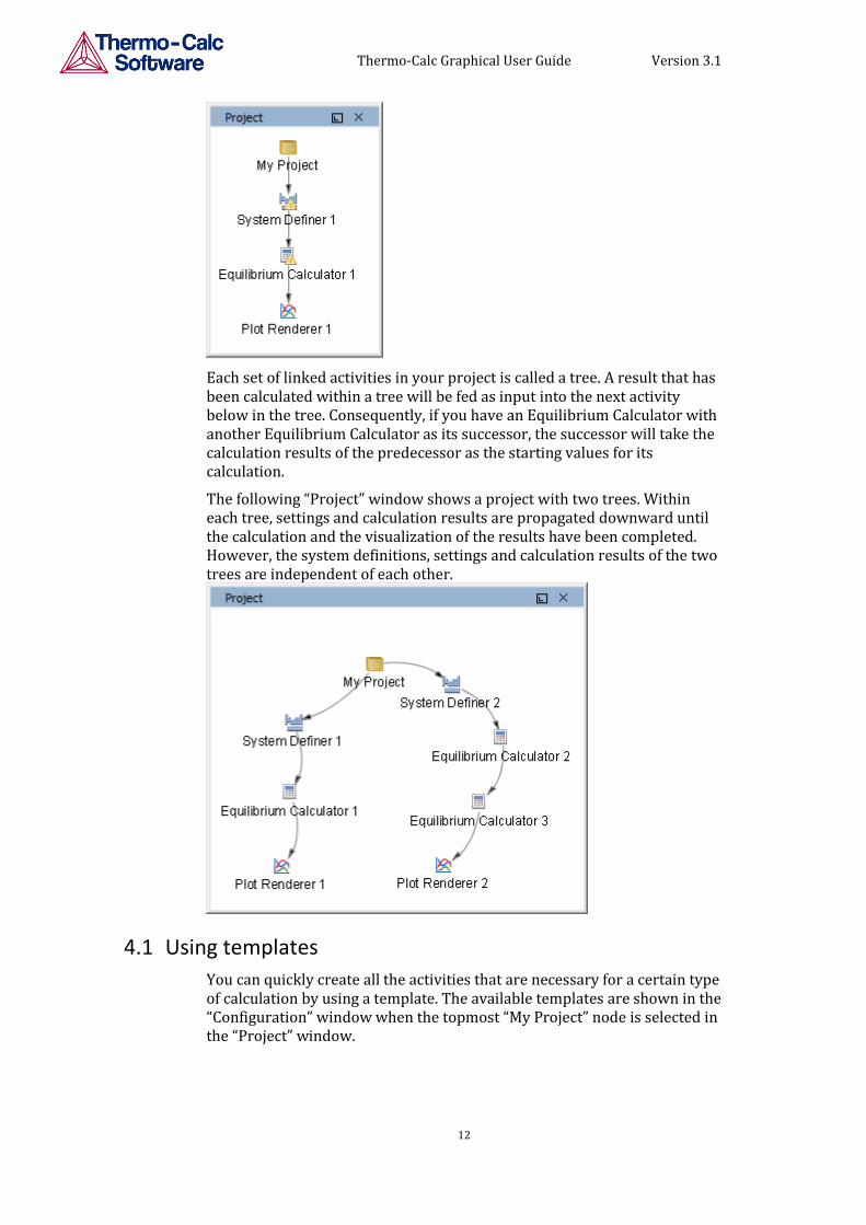
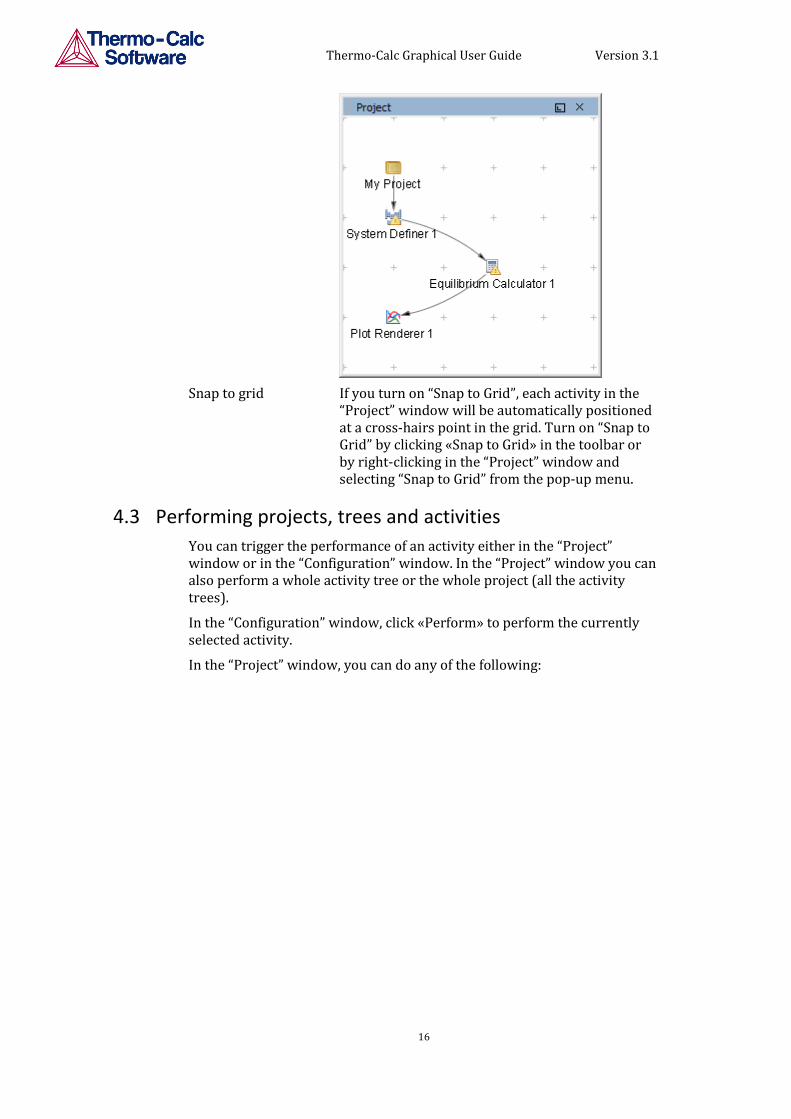
You work with Thermo-Calc in the Graphical mode by creating, configuring and performing activities within a project. The activities in your project and how they are linked are represented as a tree-structure in the Project window. This window is also where you add new activities. An activity that is located below another activity in a tree is referred to as that activity’s ‘successor’. An activity that is located above another activity in a tree is referred to as that activity’s ‘predecessor’. A predecessor is performed before the predecessor’s successors and its result is fed forward to any successor activities.
For example, to calculate and display a phase diagram, you would create one branch with three linked activities: A System Definer activity linked to an Equilibrium Calculator activity, which in turn would be connected to a Plot Renderer activity.
In the following “Project” window, “Equilibrium Calculator 1” is the successor to “System Definer 1” and the predecessor to “Plot Renderer 1”
Thermo-Calc Graphical User Guide Version 3.1
12
Each set of linked activities in your project is called a tree. A result that has been calculated within a tree will be fed as input into the next activity below in the tree. Consequently, if you have an Equilibrium Calculator with another Equilibrium Calculator as its successor, the successor will take the calculation results of the predecessor as the starting values for its calculation.
The following “Project” window shows a project with two trees. Within each tree, settings and calculation results are propagated downward until the calculation and the visualization of the results have been completed. However, the system definitions, settings and calculation results of the two trees are independent of each other.
4.1 Using templates
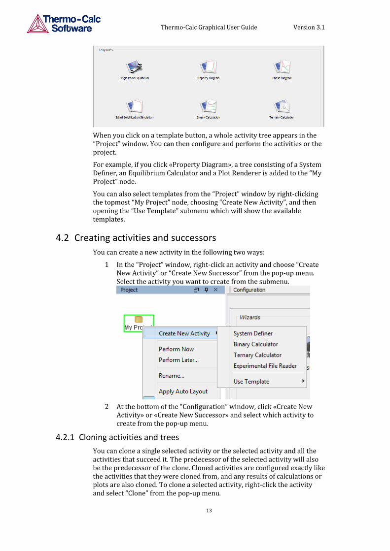
You can quickly create all the activities that are necessary for a certain type of calculation by using a template. The available templates are shown in the “Configuration” window when the topmost “My Project” node is selected in the “Project” window.
Thermo-Calc Graphical User Guide Version 3.1
13
When you click on a template button, a whole activity tree appears in the “Project” window. You can then configure and perform the activities or the project.
For example, if you click «Property Diagram», a tree consisting of a System Definer, an Equilibrium Calculator and a Plot Renderer is added to the “My Project” node.
You can also select templates from the “Project” window by right-clicking the topmost “My Project” node, choosing “Create New Activity”, and then opening the “Use Template” submenu which will show the available templates.
4.2 Creating activities and successors
You can create a new activity in the following two ways:
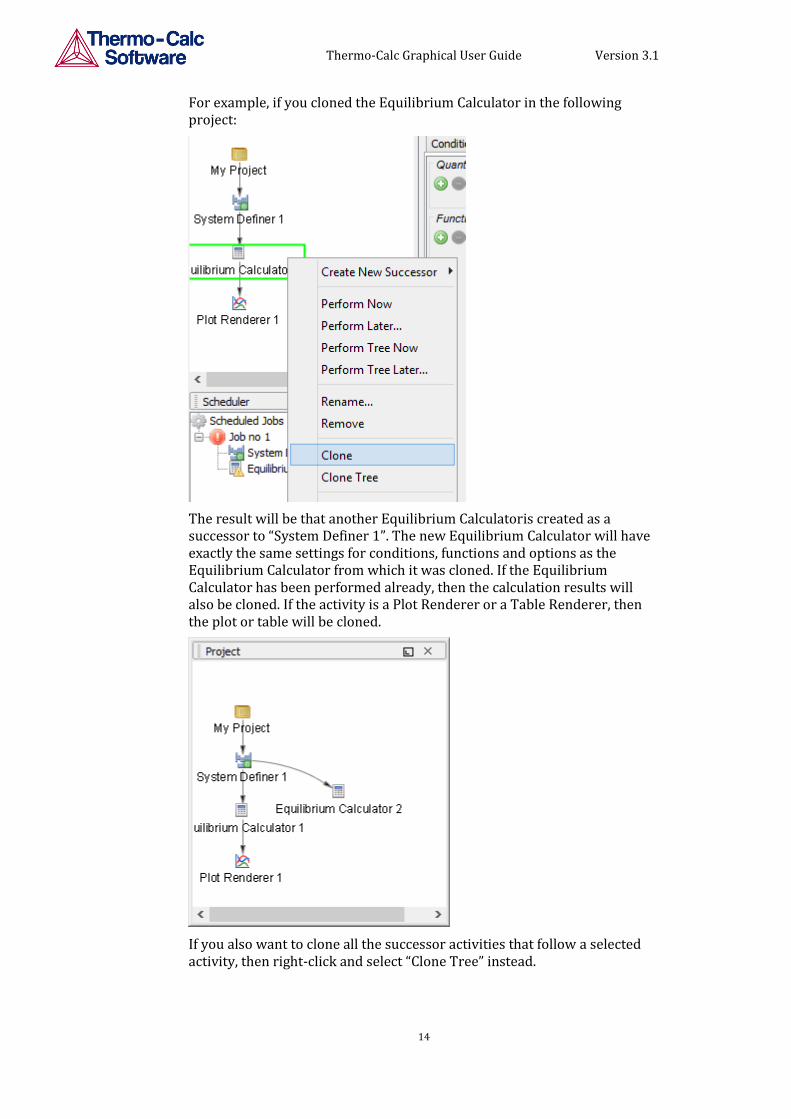
1 In the “Project” window, right-click an activity and choose “Create New Activity” or “Create New Successor” from the pop-up menu. Select the activity you want to create from the submenu.
2 At the bottom of the “Configuration” window, click «Create New Activity» or «Create New Successor» and select which activity to create from the pop-up menu.
4.2.1 Cloning activities and trees
You can clone a single selected activity or the selected activity and all the activities that succeed it. The predecessor of the selected activity will also be the predecessor of the clone. Cloned activities are configured exactly like the activities that they were cloned from, and any results of calculations or plots are also cloned. To clone a selected activity, right-click the activity and select “Clone” from the pop-up menu.
Thermo-Calc Graphical User Guide Version 3.1
14
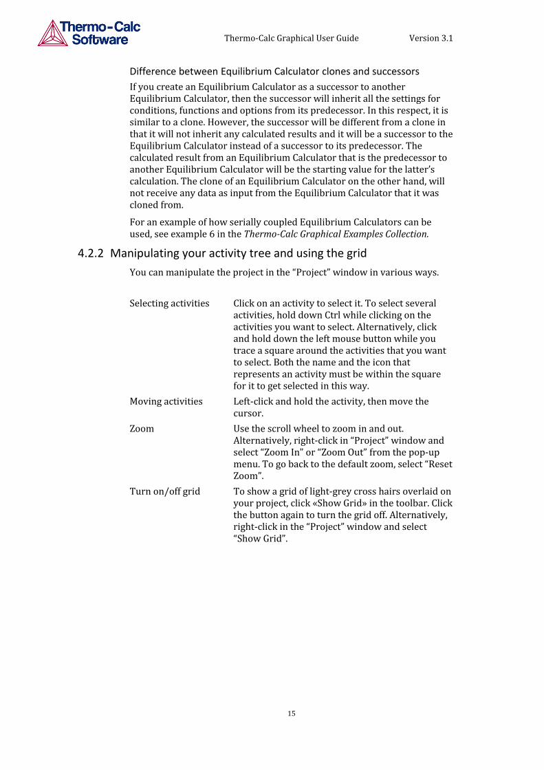
For example, if you cloned the Equilibrium Calculator in the following project:
The result will be that another Equilibrium Calculatoris created as a successor to “System Definer 1”. The new Equilibrium Calculator will have exactly the same settings for conditions, functions and options as the Equilibrium Calculator from which it was cloned. If the Equilibrium Calculator has been performed already, then the calculation results will also be cloned. If the activity is a Plot Renderer or a Table Renderer, then the plot or table will be cloned.
If you also want to clone all the successor activities that follow a selected activity, then right-click and select “Clone Tree” instead.
Thermo-Calc Graphical User Guide Version 3.1
15
Difference between Equilibrium Calculator clones and successors
If you create an Equilibrium Calculator as a successor to another Equilibrium Calculator, then the successor will inherit all the settings for conditions, functions and options from its predecessor. In this respect, it is similar to a clone. However, the successor will be different from a clone in that it will not inherit any calculated results and it will be a successor to the Equilibrium Calculator instead of a successor to its predecessor. The calculated result from an Equilibrium Calculator that is the predecessor to another Equilibrium Calculator will be the starting value for the latter’s calculation. The clone of an Equilibrium Calculator on the other hand, will not receive any data as input from the Equilibrium Calculator that it was cloned from.
For an example of how serially coupled Equilibrium Calculators can be used, see example 6 in the Thermo-Calc Graphical Examples Collection.
4.2.2 Manipulating your activity tree and using the grid
You can manipulate the project in the “Project” window in various ways.
Selecting activities Click on an activity to select it. To select several activities, hold down Ctrl while clicking on the activities you want to select. Alternatively, click and hold down the left mouse button while you trace a square around the activities that you want to select. Both the name and the icon that represents an activity must be within the square for it to get selected in this way.
Moving activities Left-click and hold the activity, then move the cursor.
Zoom Use the scroll wheel to zoom in and out. Alternatively, right-click in “Project” window and select “Zoom In” or “Zoom Out” from the pop-up menu. To go back to the default zoom, select “Reset Zoom”.
Turn on/off grid To show a grid of light-grey cross hairs overlaid on your project, click «Show Grid» in the toolbar. Click the button again to turn the grid off. Alternatively, right-click in the “Project” window and select “Show Grid”.
Thermo-Calc Graphical User Guide Version 3.1
16
Snap to grid If you turn on “Snap to Grid”, each activity in the “Project” window will be automatically positioned at a cross-hairs point in the grid. Turn on “Snap to Grid” by clicking «Snap to Grid» in the toolbar or by right-clicking in the “Project” window and selecting “Snap to Grid” from the pop-up menu.
4.3 Performing projects, trees and activities
You can trigger the performance of an activity either in the “Project” window or in the “Configuration” window. In the “Project” window you can also perform a whole activity tree or the whole project (all the activity trees).
In the “Configuration” window, click «Perform» to perform the currently selected activity.
In the “Project” window, you can do any of the following:
Thermo-Calc Graphical User Guide Version 3.1
17
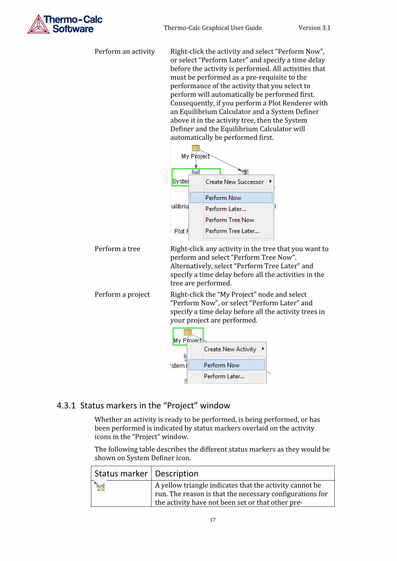
Perform an activity Right-click the activity and select “Perform Now”, or select “Perform Later” and specify a time delay before the activity is performed. All activities that must be performed as a pre-requisite to the performance of the activity that you select to perform will automatically be performed first. Consequently, if you perform a Plot Renderer with an Equilibrium Calculator and a System Definer above it in the activity tree, then the System Definer and the Equilibrium Calculator will automatically be performed first.
Perform a tree Right-click any activity in the tree that you want to perform and select “Perform Tree Now”. Alternatively, select “Perform Tree Later” and specify a time delay before all the activities in the tree are performed.
Perform a project Right-click the “My Project” node and select “Perform Now”, or select “Perform Later” and specify a time delay before all the activity trees in your project are performed.
4.3.1 Status markers in the “Project” window
Whether an activity is ready to be performed, is being performed, or has been performed is indicated by status markers overlaid on the activity icons in the “Project” window.
The following table describes the different status markers as they would be shown on System Definer icon.
Status marker Description
A yellow triangle indicates that the activity cannot be run. The reason is that the necessary configurations for the activity have not been set or that other pre-
Thermo-Calc Graphical User Guide Version 3.1
18
requisites have not been met.
No status marker means that the activity is ready to be performed and that it has not yet been performed.
A red circle with a dial (a clock face) indicates that the activity is currently being performed.
A green disc indicates that the activity has been performed.
4.3.2 Using the Scheduler
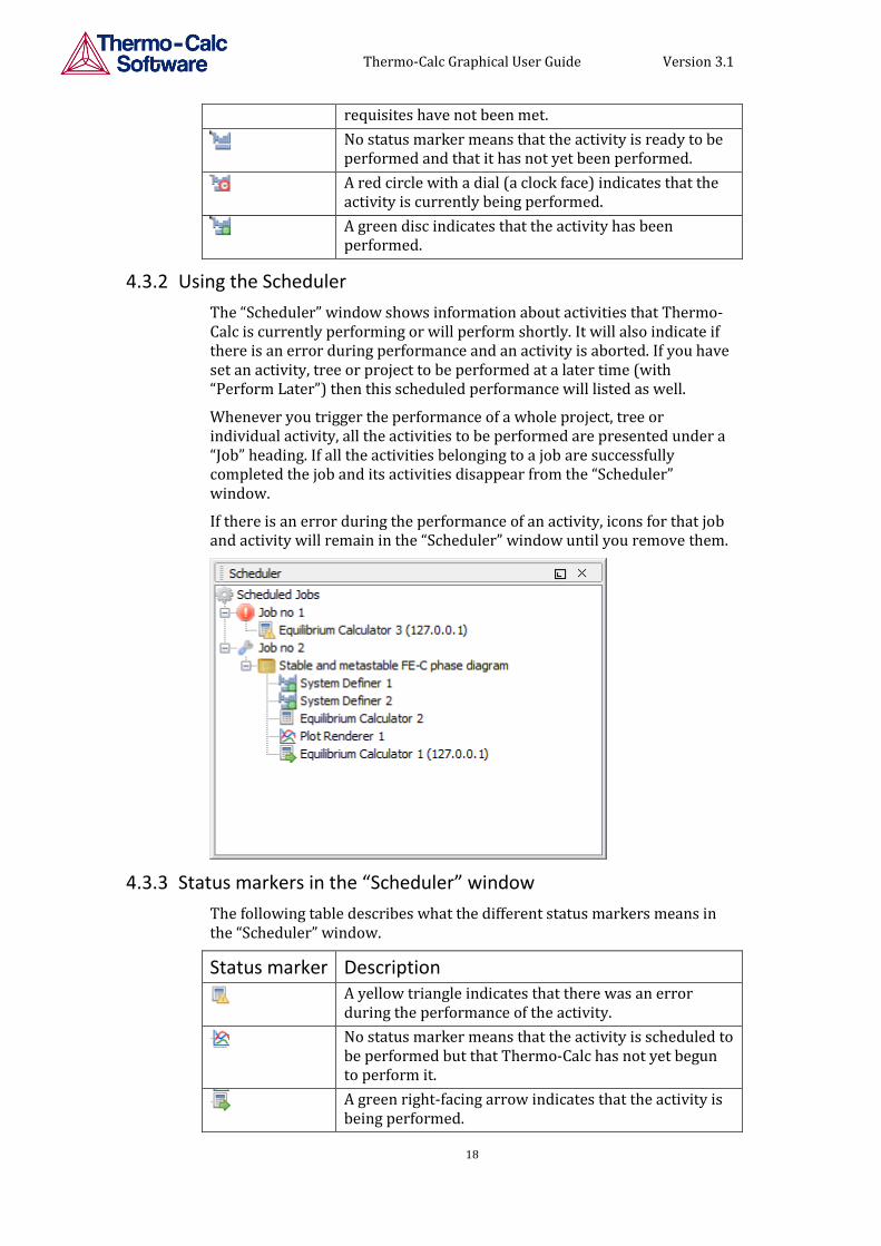
The “Scheduler” window shows information about activities that Thermo-Calc is currently performing or will perform shortly. It will also indicate if there is an error during performance and an activity is aborted. If you have set an activity, tree or project to be performed at a later time (with “Perform Later”) then this scheduled performance will listed as well.
Whenever you trigger the performance of a whole project, tree or individual activity, all the activities to be performed are presented under a “Job” heading. If all the activities belonging to a job are successfully completed the job and its activities disappear from the “Scheduler” window.
If there is an error during the performance of an activity, icons for that job and activity will remain in the “Scheduler” window until you remove them.
4.3.3 Status markers in the “Scheduler” window
The following table describes what the different status markers means in the “Scheduler” window.
Status marker Description
A yellow triangle indicates that there was an error during the performance of the activity.
No status marker means that the activity is scheduled to be performed but that Thermo-Calc has not yet begun to perform it.
A green right-facing arrow indicates that the activity is being performed.
Thermo-Calc Graphical User Guide Version 3.1
19
A green disc indicates that the activity has already been performed successfully.
4.3.4 Managing the schedule
In the “Scheduler” window, you can cancel scheduled jobs, remove errors and show information about errors.
“Cancel All Jobs” To cancel all jobs, right-click the “Scheduled Jobs” label or the cogwheel icon, then select “Cancel All Jobs” from the pop-up menu.
“Clear All Errors” To remove all failed activities and jobs, right-click the “Scheduled Jobs” label or the cogwheel icon, then select “Clear All Errors” from the pop-up menu.
“Cancel Job” To cancel one specific job, right-click the job label (for example, “Job no 1”) and select “Cancel Job” from the pop-up menu.
“Clear Error” To remove a specific failed job, right-click the job label (for example, “Job no 1”) and select “Cancel Job” from the pop-up menu.
“Show Error Log” To open a window with information about an error, right-click the label for the failed job (for example, “Job no 1”), and select “Show Error Log”.
4.3.5 The Event Log
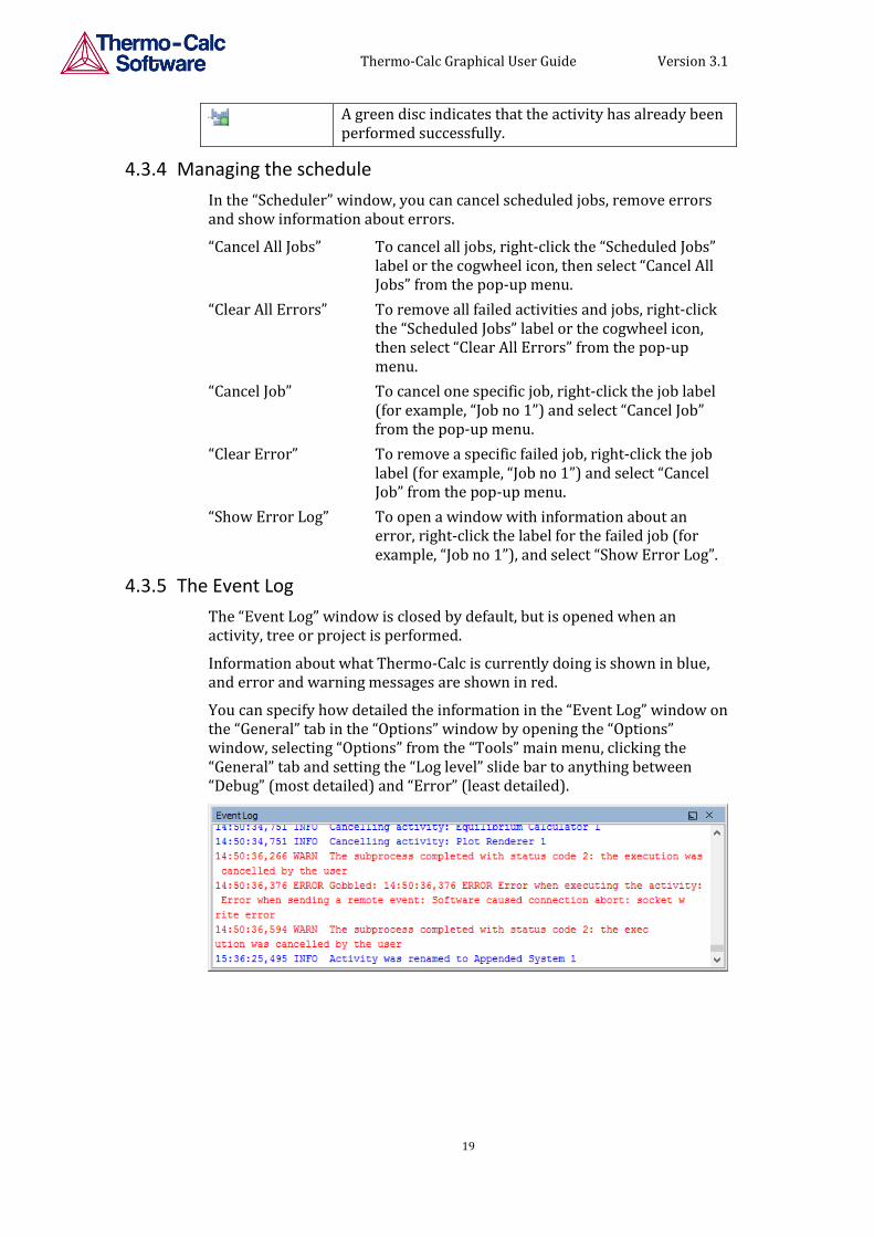
The “Event Log” window is closed by default, but is opened when an activity, tree or project is performed.
Information about what Thermo-Calc is currently doing is shown in blue, and error and warning messages are shown in red.
You can specify how detailed the information in the “Event Log” window on the “General” tab in the “Options” window by opening the “Options” window, selecting “Options” from the “Tools” main menu, clicking the “General” tab and setting the “Log level” slide bar to anything between “Debug” (most detailed) and “Error” (least detailed).
Thermo-Calc Graphical User Guide Version 3.1
20
4.4 Using Thermo-Calc project files
Thermo-Calc makes use of project files with the file name suffix .TCU. To save your project and all its settings and results, click «Save» on the toolbar. In the “Save” window that opens, you can select whether or not to “Include calculated results in the project file” (by default, this is selected). To open a Thermo-Calc project file, click «Open» on the toolbar and select the project file in the “Open file” window.
You can only have one project file open at a time. However, you can attach the trees from additional project files to the topmost “My Project” node. To append an additional project file in this way, select “Append Project” from the “File” main menu and then open a project file of your choice.
5 The activities
In this chapter, you find a description of each type of activity, brief descriptions of the “Configuration” window settings, and descriptions of some procedures that are tied to specific activities.
5.1 System definer
In a System Definer activity, you select which database to use for retrieving thermodynamic data, and define which elements your system will have as components. You can also select which species to include as well as change the reference temperature and pressure for your components.
5.1.1 Predecessors and successors
Possible predecessors My Project System Definer
Possible successors System Definer Equilibrium Calculator Scheil Calculator
A System Definer that is a successor to another System Definer by default gets the name “Appended System”.
5.1.2 How to select a database and define your elements
This procedure describes the procedure you need to go through to define your system, namely select a database and defining the elements that will be in your system.
Pre-requisites
You must have created and selected a System Definer activity in the “Project” window.
Procedure
To define your system, follow these steps:
Step Action
1 In the “Configuration” window, select the database you want to use from the “Select database” menu near the top of the window.
Thermo-Calc Graphical User Guide Version 3.1
21
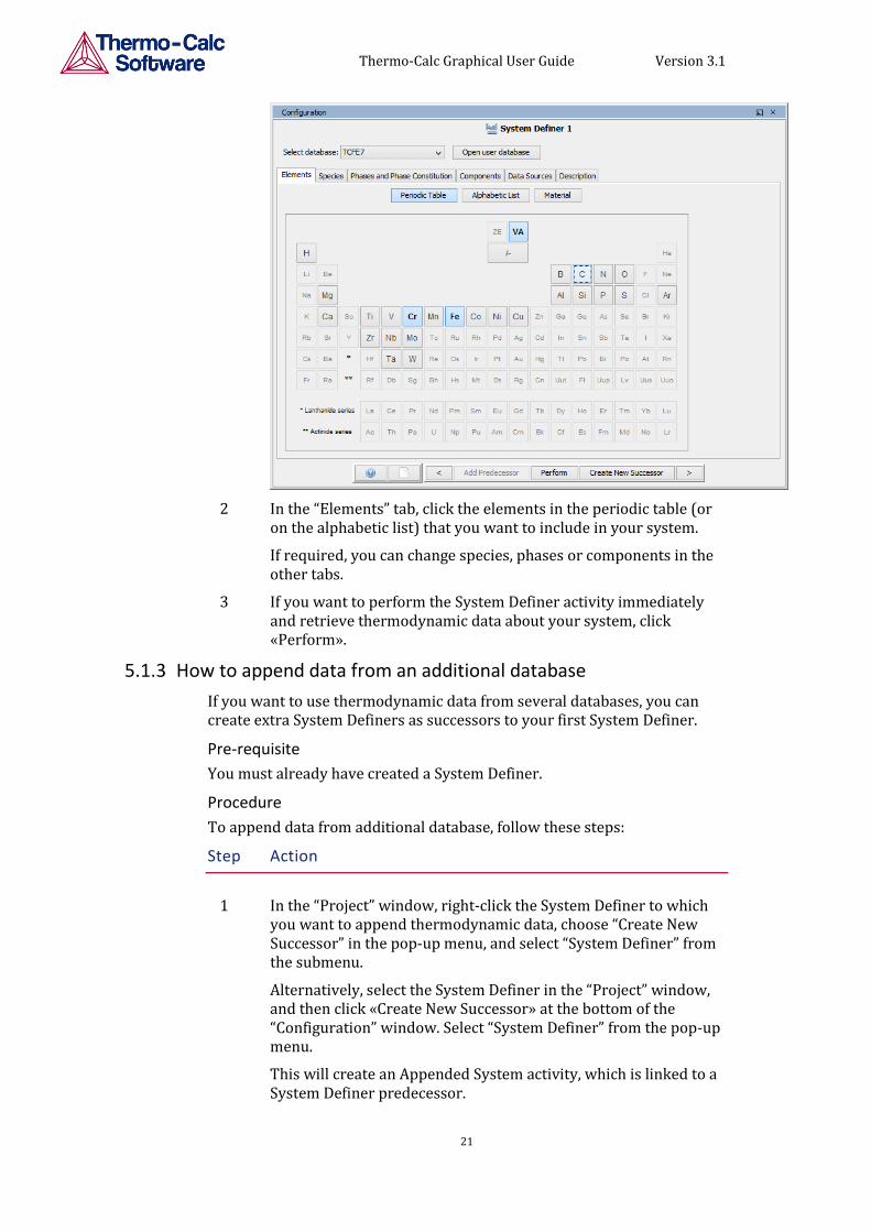
2 In the “Elements” tab, click the elements in the periodic table (or on the alphabetic list) that you want to include in your system.
If required, you can change species, phases or components in the other tabs.
3 If you want to perform the System Definer activity immediately and retrieve thermodynamic data about your system, click «Perform».
5.1.3 How to append data from an additional database
If you want to use thermodynamic data from several databases, you can create extra System Definers as successors to your first System Definer.
Pre-requisite
You must already have created a System Definer.
Procedure
To append data from additional database, follow these steps:
Step Action
1 In the “Project” window, right-click the System Definer to which you want to append thermodynamic data, choose “Create New Successor” in the pop-up menu, and select “System Definer” from the submenu.
Alternatively, select the System Definer in the “Project” window, and then click «Create New Successor» at the bottom of the “Configuration” window. Select “System Definer” from the pop-up menu.
This will create an Appended System activity, which is linked to a System Definer predecessor.
Thermo-Calc Graphical User Guide Version 3.1
22
2 In the “Configuration” window for the Appended System, select which database you want to append thermodynamic data from, regarding which components, phases, etc.
5.2 Equilibrium Calculator
An Equilibrium Calculator allows you to set the conditions for, and perform, a calculation. The “Configuration” window for an Equilibrium Calculator has three tabs:
“Conditions” tab Here you set the conditions for your calculation that define the stepping or mapping axis variables. This tab can be viewed in a simplified mode and in an advanced mode.
“Functions” tab Here you define your own quantities and functions, which you then can calculate and plot.
“Options” tab Here you can modify various numerical settings that determine how equilibria are calculated, as well as how stepping and mapping calculations are performed.
5.2.1 Predecessors and successors
Possible predecessors System Definer Equilibrium Calculator
Possible successors Plot Renderer Table Renderer Equilibrium Calculator
An Equilibrium Calculator that is the successor of another Equilibrium Calculator inherits all the “Configuration” window settings of the predecessor.
For an example of how serially coupled Equilibrium Calculators can be used, see example 6 in the Thermo-Calc Graphical Examples Collection.
5.2.2 Setting conditions for different calculations
Conditions and axis variables are set in the “Conditions” tab of the “Configuration” window. There you can specify the conditions and axis variables you want to use for your calculation. The tab can be viewed in two modes, the simplified mode (default) or the advanced mode.
What conditions you have to set depends on the type of calculation you intend to perform.
For examples of how various kinds of calculations can be set up using an Equilibrium Calculator, see the Thermo-Calc Graphical Examples Collection: example 1 is an example of a single-point equilibrium calculation; example 2 an example of a stepping calculation; and example 5 is an example of a mapping calculation.
Thermo-Calc Graphical User Guide Version 3.1
23
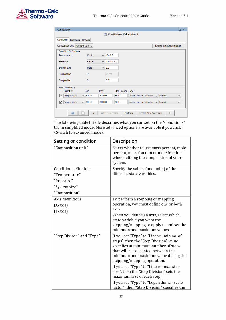
The following table briefly describes what you can set on the “Conditions” tab in simplified mode. More advanced options are available if you click «Switch to advanced mode».
Setting or condition Description “Composition unit” Select whether to use mass percent, mole
percent, mass fraction or mole fraction when defining the composition of your system.
Condition definitions
“Temperature”
“Pressure”
“System size”
“Composition”
Specify the values (and units) of the different state variables.
Axis definitions
(X-axis)
(Y-axis)
To perform a stepping or mapping operation, you must define one or both axes.
When you define an axis, select which state variable you want the stepping/mapping to apply to and set the minimum and maximum values.
“Step Divison” and “Type” If you set “Type” to “Linear - min no. of steps”, then the “Step Division” value specifies at minimum number of steps that will be calculated between the minimum and maximum value during the stepping/mapping operation.
If you set “Type” to “Linear - max step size”, then the “Step Division” sets the maximum size of each step.
If you set “Type” to “Logarithmic - scale factor”, then “Step Division” specifies the
Thermo-Calc Graphical User Guide Version 3.1
24
scale factor of a logarithmic function that distributes the steps from the initial equilibrium to the minimum and maximum values you have defines.
“Normal” / “Separate phases” / “T-Zero”
To do the stepping operation along an axis one phase at a time, select “Separate phases”.
If you want to calculate the T0-line, where the Gibbs energy for each phase is the same, then select “T-Zero”.
5.2.3 Setting conditions – advanced mode
In advanced mode, you can add and remove conditions as you see fit. Furthermore, you can define additional axis definitions beyond the two that you can set in simplified mode. However, the number and types of conditions that you set must still conform to the Gibbs’ phase rule (see Thermo-Calc Educational Material). The “Number of missing conditions is” field, at the top of the tab shows how many conditions that you have left to set. If the number is negative, then you need to remove that number of conditions.
The next section demonstrates how to calculate and plot a diagram with a fixed phase in order to find out, for example, at what temperature a material starts to melt.
5.2.4 How to calculate with a fixed phase
This section describes how you use the advanced mode to set a certain phase to be fixed at a certain amount. This allows you to, for example, find out at what temperature you material starts to melt. If you set the phase to be fixed to liquid phase at zero amount, and leave the temperature state variable undefined, then you can calculate at what temperature your material will enter a state where the liquid phase is no longer zero (that is when it will start to melt).
When you perform an equilibrium calculation with a fixed phase, it is recommend that you do this in an Equilibrium Calculator that is the successor to an Equilibrium Calculator that performs an ordinary equilibrium calculation for which you roughly estimate the value of the condition you are interested in. This will provide your fixed phase calculation with better starting values.
Pre-requisites
You must have created an Equilibrium Calculator and you must have this activity selected in the “Project” window.
Procedure
To make a calculation with a fixed phase, follow these steps:
Step Action
1 In the “Configuration” window, click «Switch to advanced mode».
Thermo-Calc Graphical User Guide Version 3.1
25
If you have set “Default calculation mode” to “Advanced” in the “Calculation” tab of the “Options” window, then the “Configuration” window will be in advanced mode by default, see section 2.3.
2 Click the green “+” button to add a condition.
3 Select “Fix phase” from the first menu.
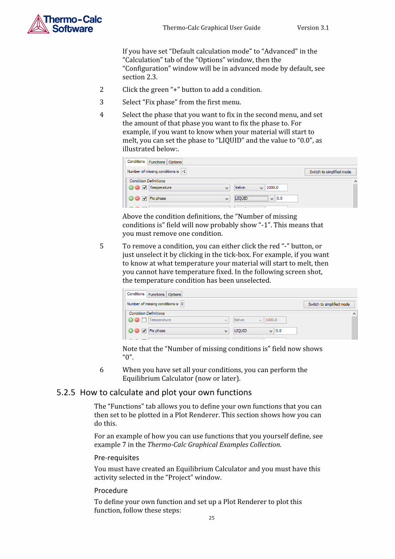
4 Select the phase that you want to fix in the second menu, and set the amount of that phase you want to fix the phase to. For example, if you want to know when your material will start to melt, you can set the phase to “LIQUID” and the value to “0.0”, as illustrated below:.
Above the condition definitions, the “Number of missing conditions is” field will now probably show “-1”. This means that you must remove one condition.
5 To remove a condition, you can either click the red “-” button, or just unselect it by clicking in the tick-box. For example, if you want to know at what temperature your material will start to melt, then you cannot have temperature fixed. In the following screen shot, the temperature condition has been unselected.
Note that the “Number of missing conditions is” field now shows “0”.
6 When you have set all your conditions, you can perform the Equilibrium Calculator (now or later).
5.2.5 How to calculate and plot your own functions
The “Functions” tab allows you to define your own functions that you can then set to be plotted in a Plot Renderer. This section shows how you can do this.
For an example of how you can use functions that you yourself define, see example 7 in the Thermo-Calc Graphical Examples Collection.
Pre-requisites
You must have created an Equilibrium Calculator and you must have this activity selected in the “Project” window.
Procedure
To define your own function and set up a Plot Renderer to plot this function, follow these steps:
Thermo-Calc Graphical User Guide Version 3.1
26
Step Action
1 In the “Configuration” window, click the “Functions” tab.
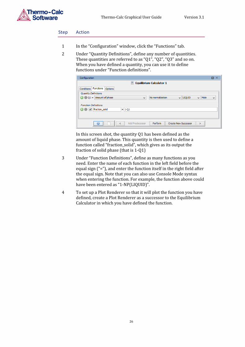
2 Under “Quantity Definitions”, define any number of quantities. These quantities are referred to as “Q1”, “Q2”, “Q3” and so on. When you have defined a quantity, you can use it to define functions under “Function definitions”.
In this screen shot, the quantity Q1 has been defined as the amount of liquid phase. This quantity is then used to define a function called “fraction_solid”, which gives as its output the fraction of solid phase (that is 1-Q1)
3 Under “Function Definitions”, define as many functions as you need. Enter the name of each function in the left field before the equal sign (“=”), and enter the function itself in the right field after the equal sign. Note that you can also use Console Mode syntax when entering the function. For example, the function above could have been entered as “1-NP(LIQUID)”.
4 To set up a Plot Renderer so that it will plot the function you have defined, create a Plot Renderer as a successor to the Equilibrium Calculator in which you have defined the function.
Thermo-Calc Graphical User Guide Version 3.1
27
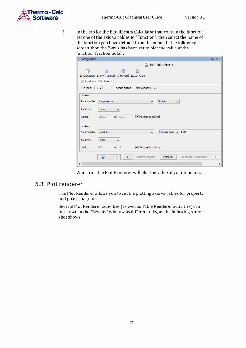
5 In the tab for the Equilibrium Calculator that contain the function, set one of the axis variables to “Function”, then select the name of the function you have defined from the menu. In the following screen shot, the Y-axis has been set to plot the value of the function “fraction_solid”.
When run, the Plot Renderer will plot the value of your function.
5.3 Plot renderer
The Plot Renderer allows you to set the plotting axis variables for property and phase diagrams.
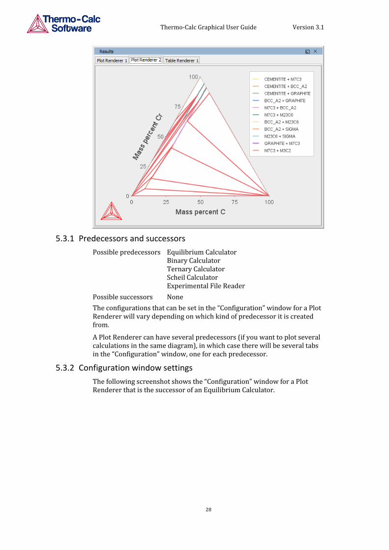
Several Plot Renderer activities (as well as Table Renderer activities) can be shown in the “Results” window as different tabs, as the following screen shot shows:
Thermo-Calc Graphical User Guide Version 3.1
28
5.3.1 Predecessors and successors
Possible predecessors Equilibrium Calculator Binary Calculator Ternary Calculator Scheil Calculator Experimental File Reader
Possible successors None
The configurations that can be set in the “Configuration” window for a Plot Renderer will vary depending on which kind of predecessor it is created from.
A Plot Renderer can have several predecessors (if you want to plot several calculations in the same diagram), in which case there will be several tabs in the “Configuration” window, one for each predecessor.
5.3.2 Configuration window settings
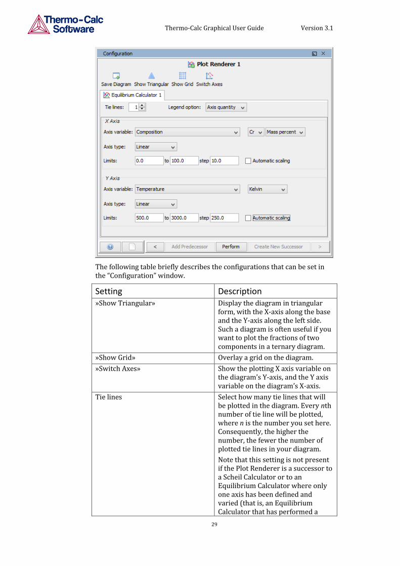
The following screenshot shows the “Configuration” window for a Plot Renderer that is the successor of an Equilibrium Calculator.
Thermo-Calc Graphical User Guide Version 3.1
29
The following table briefly describes the configurations that can be set in the “Configuration” window.
Setting Description »Show Triangular» Display the diagram in triangular
form, with the X-axis along the base and the Y-axis along the left side. Such a diagram is often useful if you want to plot the fractions of two components in a ternary diagram.
»Show Grid» Overlay a grid on the diagram.
»Switch Axes» Show the plotting X axis variable on the diagram’s Y-axis, and the Y axis variable on the diagram’s X-axis.
Tie lines Select how many tie lines that will be plotted in the diagram. Every nth number of tie line will be plotted, where n is the number you set here. Consequently, the higher the number, the fewer the number of plotted tie lines in your diagram.
Note that this setting is not present if the Plot Renderer is a successor to a Scheil Calculator or to an Equilibrium Calculator where only one axis has been defined and varied (that is, an Equilibrium Calculator that has performed a
Thermo-Calc Graphical User Guide Version 3.1
30
stepping calculation).
Legend option Select whether the diagram’s legend should display the “Stable phases” or the “Axis quantity”.
Axis variable Set which state variable that you want plotted along the X-axis and the Y-axis.
Axis type Select what type of scale to use on the axis. Choose between “Linear”, “Logarithmic”, “Logarithmic 10” or “Inverse”.
Limits Specify the range along the axis that should be shown in the plot by setting the minimum and maximum values of the axis variable. You can also determine the step size between the tick marks along each axis.
Alternatively, select “Automatic scaling”.
5.3.3 Changing the appearance of a plotted diagram
To change the appearance of your diagram, right click on the diagram and select “Properties” from the pop-up menu. This will open up a Plot Properties window. Here you can, for example, change the fonts and colours used, and enter a title for your diagram.
You can also change the colour, stroke (solid/dashed/dotted/dash_dot) and line width of a particular series of lines in the plot by double-clicking one of the lines in the series. In this way, you can also toggle whether data points should be shown or not for a series of lines. The crosshair cursor turns into a cursor resembling a pointing hand when it is placed over a line that can clicked but if you hold down Ctrl, this will not happen (the cursor will continue to be shown as a crosshair).
To configure the default settings for plotting, select “Options” from the “Tools” main menu and open the “Plotting” tab under Graphical Mode>Activities.
5.3.4 Adding labels
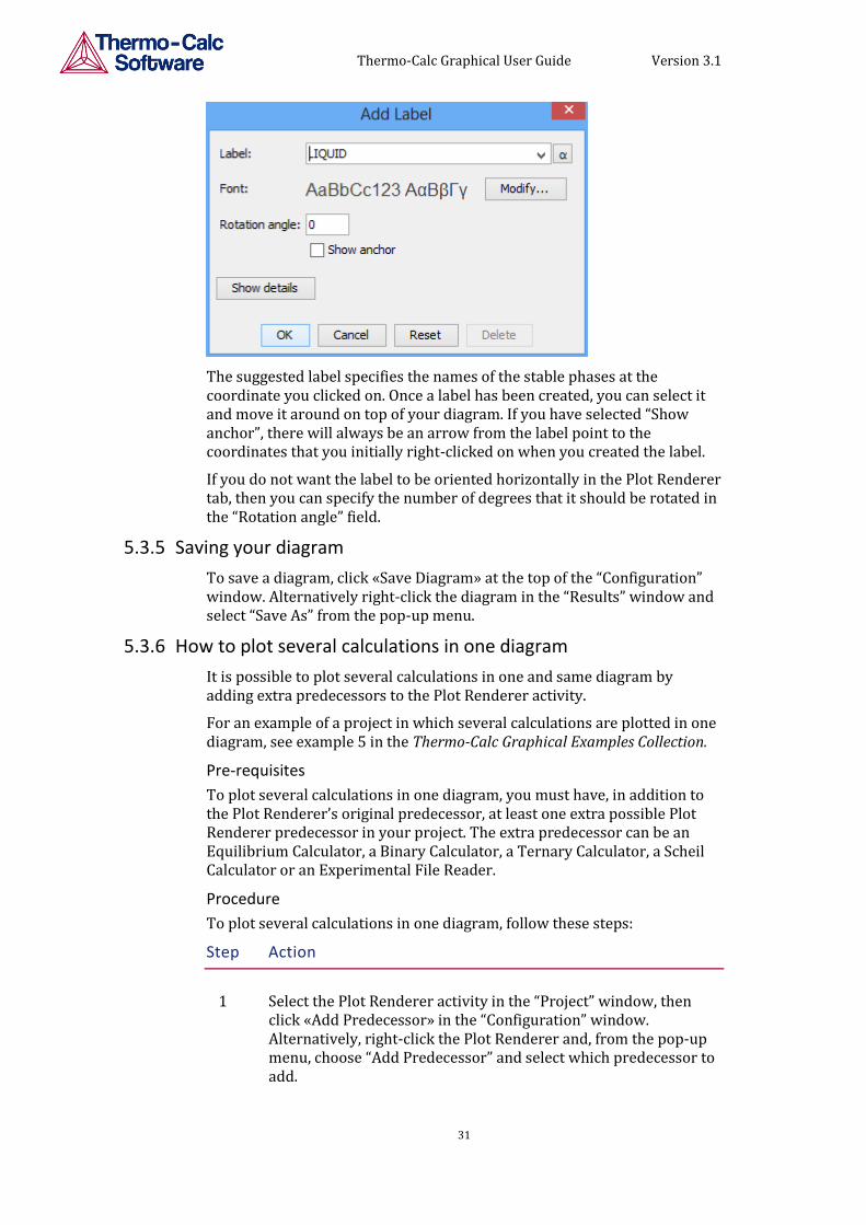
To add a label text at a certain point in the diagram, right click on that point, and select “Add Label” from the pop-up menu. This will open the “Add Label” window.
Thermo-Calc Graphical User Guide Version 3.1
31
The suggested label specifies the names of the stable phases at the coordinate you clicked on. Once a label has been created, you can select it and move it around on top of your diagram. If you have selected “Show anchor”, there will always be an arrow from the label point to the coordinates that you initially right-clicked on when you created the label.
If you do not want the label to be oriented horizontally in the Plot Renderer tab, then you can specify the number of degrees that it should be rotated in the “Rotation angle” field.
5.3.5 Saving your diagram
To save a diagram, click «Save Diagram» at the top of the “Configuration” window. Alternatively right-click the diagram in the “Results” window and select “Save As” from the pop-up menu.
5.3.6 How to plot several calculations in one diagram
It is possible to plot several calculations in one and same diagram by adding extra predecessors to the Plot Renderer activity.
For an example of a project in which several calculations are plotted in one diagram, see example 5 in the Thermo-Calc Graphical Examples Collection.
Pre-requisites
To plot several calculations in one diagram, you must have, in addition to the Plot Renderer’s original predecessor, at least one extra possible Plot Renderer predecessor in your project. The extra predecessor can be an Equilibrium Calculator, a Binary Calculator, a Ternary Calculator, a Scheil Calculator or an Experimental File Reader.
Procedure
To plot several calculations in one diagram, follow these steps:
Step Action
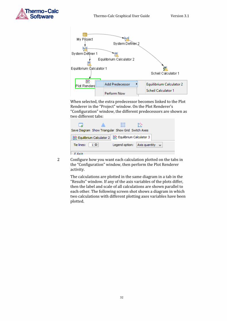
1 Select the Plot Renderer activity in the “Project” window, then click «Add Predecessor» in the “Configuration” window. Alternatively, right-click the Plot Renderer and, from the pop-up menu, choose “Add Predecessor” and select which predecessor to add.
Thermo-Calc Graphical User Guide Version 3.1
32
When selected, the extra predecessor becomes linked to the Plot Renderer in the “Project” window. On the Plot Renderer’s “Configuration” window, the different predecessors are shown as two different tabs:
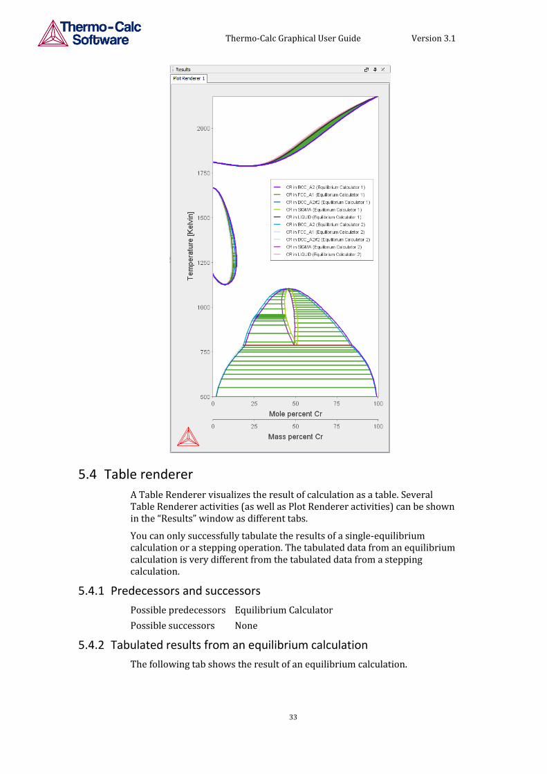
2 Configure how you want each calculation plotted on the tabs in the “Configuration” window, then perform the Plot Renderer activity.
The calculations are plotted in the same diagram in a tab in the “Results” window. If any of the axis variables of the plots differ, then the label and scale of all calculations are shown parallel to each other. The following screen shot shows a diagram in which two calculations with different plotting axes variables have been plotted.
Thermo-Calc Graphical User Guide Version 3.1
33
5.4 Table renderer
A Table Renderer visualizes the result of calculation as a table. Several Table Renderer activities (as well as Plot Renderer activities) can be shown in the “Results” window as different tabs.
You can only successfully tabulate the results of a single-equilibrium calculation or a stepping operation. The tabulated data from an equilibrium calculation is very different from the tabulated data from a stepping calculation.
5.4.1 Predecessors and successors
Possible predecessors Equilibrium Calculator
Possible successors None
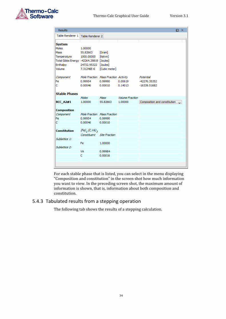
5.4.2 Tabulated results from an equilibrium calculation
The following tab shows the result of an equilibrium calculation.
Thermo-Calc Graphical User Guide Version 3.1
34
For each stable phase that is listed, you can select in the menu displaying “Composition and constitution” in the screen shot how much information you want to view. In the preceding screen shot, the maximum amount of information is shown, that is, information about both composition and constitution.
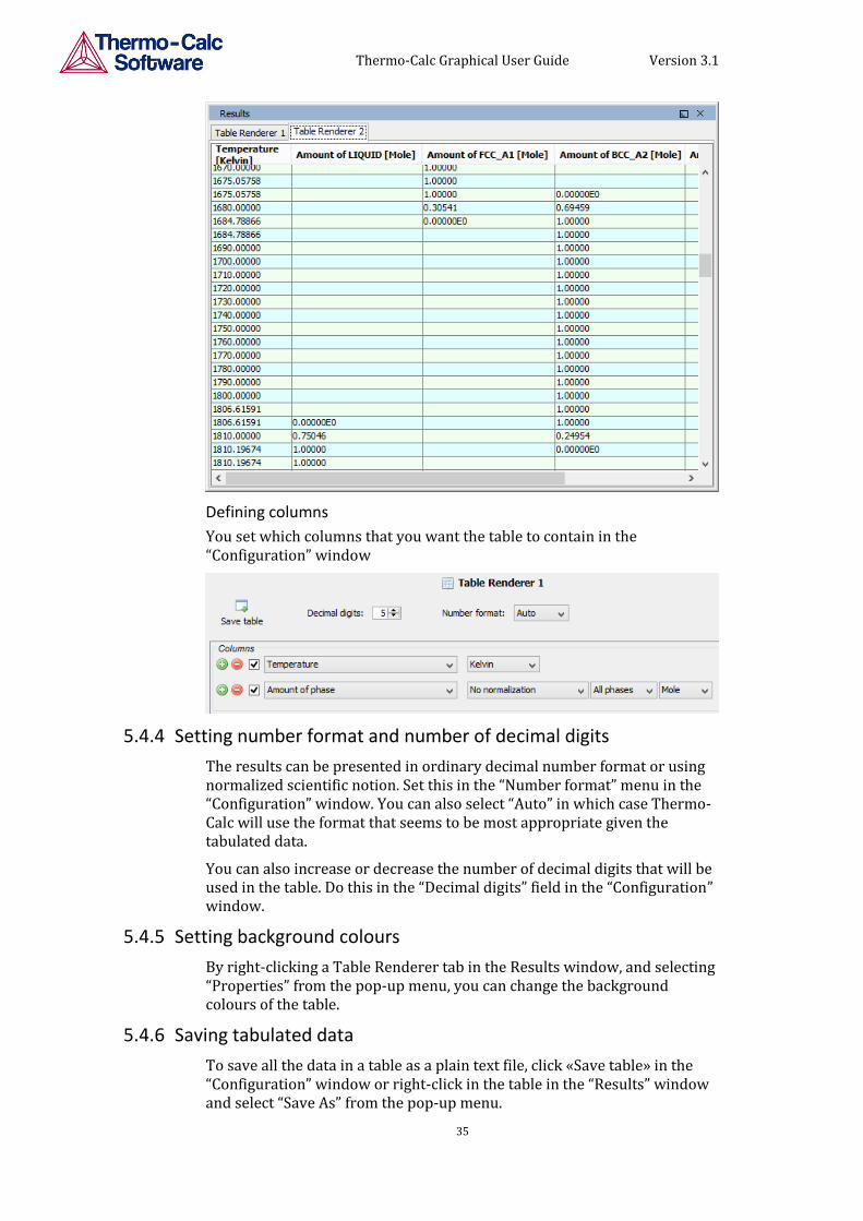
5.4.3 Tabulated results from a stepping operation
The following tab shows the results of a stepping calculation.
Thermo-Calc Graphical User Guide Version 3.1
35
Defining columns
You set which columns that you want the table to contain in the “Configuration” window
5.4.4 Setting number format and number of decimal digits
The results can be presented in ordinary decimal number format or using normalized scientific notion. Set this in the “Number format” menu in the “Configuration” window. You can also select “Auto” in which case Thermo-Calc will use the format that seems to be most appropriate given the tabulated data.
You can also increase or decrease the number of decimal digits that will be used in the table. Do this in the “Decimal digits” field in the “Configuration” window.
5.4.5 Setting background colours
By right-clicking a Table Renderer tab in the Results window, and selecting “Properties” from the pop-up menu, you can change the background colours of the table.
5.4.6 Saving tabulated data
To save all the data in a table as a plain text file, click «Save table» in the “Configuration” window or right-click in the table in the “Results” window and select “Save As” from the pop-up menu.
Thermo-Calc Graphical User Guide Version 3.1
36
To copy the data from a single cell of a table to the clipboard, right-click the cell and select “Copy” from the pop-up menu. To copy the whole table to the clipboard, select “Copy all”.
Note that data that is saved is the data that is shown in the Table Renderer tab. Data that has been calculated but which is not displayed there will not be saved.
5.5 Experimental file reader
The Experimental File Reader activity can only be created from the top “My Project” node. This activity allows you to read an experimental data file (*.EXP). Such a file contains information specifying a plotted diagram, written in the DATAPLOT graphical language. See the DATAPLOT User Guide for more information.
5.5.1 Predecessors and successors
Possible predecessors My project
Possible successors Plot Renderer
5.5.2 How to plot an experimental data file
Step Action
3 Right-click “My Project”, and choose “Experimental File Reader” from the “Create New Activity” submenu.
4 In the “EXP file” field in the “Configuration” window, enter the name of EXP-file that you want to plot.
5 Click «Create New Successor» in the “Configuration” window and select “Plot Renderer”. Alternatively: right-click the experimental file reader activity in the “Project” window and choose “Plot Renderer” from the “Create New Successor” submenu.
6 Click «Perform» in the “Configuration” window or right-click the plot renderer activity that you just created in the “Project” window.
5.6 Binary calculator
A Binary Calculator can be used for some calculations involving two components. You can think of this activity as a combination of a System Definer and an Equilibrium Calculator, but designed to simplify setting up and performing calculations on binary systems.
The Binary Calculator relies on some specifications that are not supported by all databases. You therefore need a database that was designed for the Binary Calculator, such as the TCBIN database for example.
For an example of how a Binary Calculator can be used in a project, see example 3 in the Thermo-Calc Graphical Examples Collection.
5.6.1 Predecessors and successors
Possible predecessors My Project
Possible successors Plot Renderer
Thermo-Calc Graphical User Guide Version 3.1
37
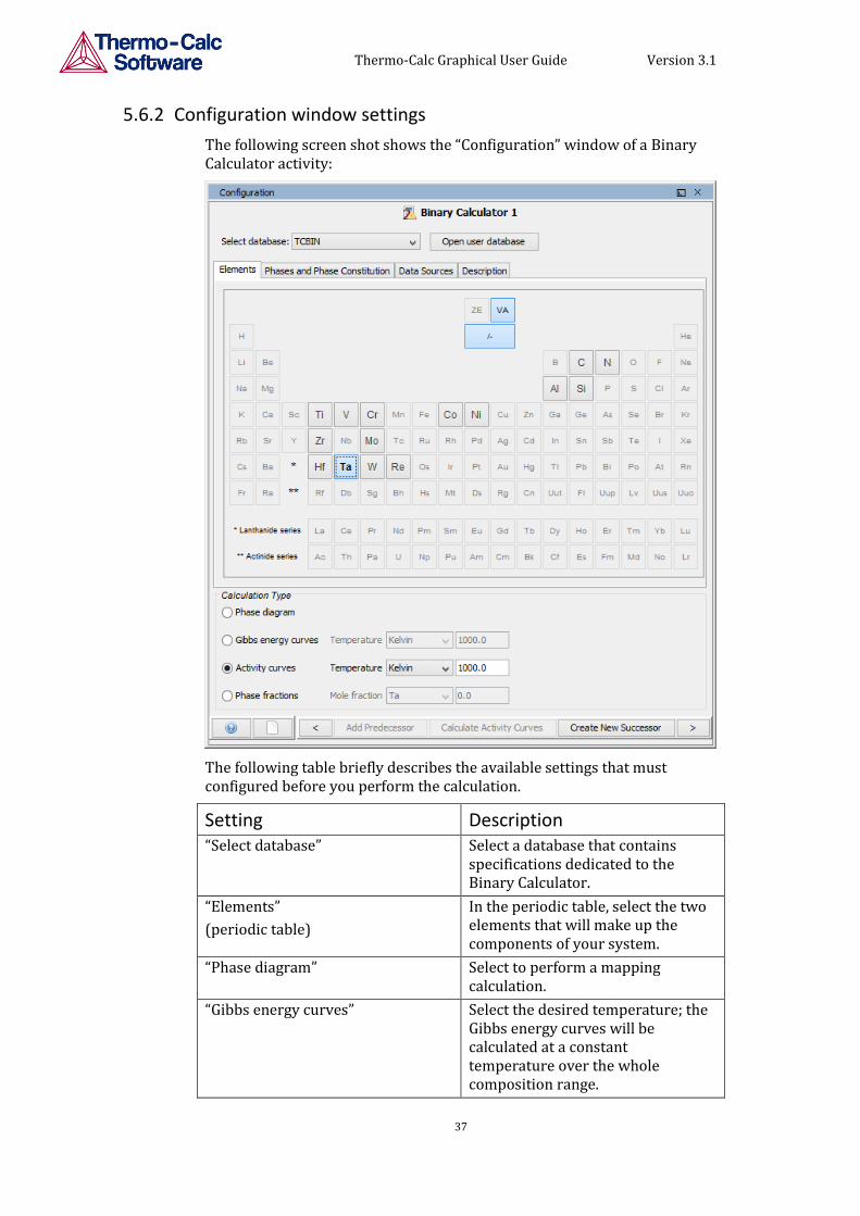
5.6.2 Configuration window settings
The following screen shot shows the “Configuration” window of a Binary Calculator activity:
The following table briefly describes the available settings that must configured before you perform the calculation.
Setting Description “Select database” Select a database that contains
specifications dedicated to the Binary Calculator.
“Elements”
(periodic table)
In the periodic table, select the two elements that will make up the components of your system.
“Phase diagram” Select to perform a mapping calculation.
“Gibbs energy curves” Select the desired temperature; the Gibbs energy curves will be calculated at a constant temperature over the whole composition range.
Thermo-Calc Graphical User Guide Version 3.1
38
“Activity curves” Select the desired temperature; the activity curves will be calculated at a constant temperature over the whole composition range.
“Phase fractions” Select the desired composition; the phase fractions will be calculated as a function of temperature at a constant composition.
5.7 Ternary calculator
A Ternary Calculator can be used for some calculations involving three components. You can think of this activity as a combination of a System Definer and an Equilibrium Calculator, but designed to simplify setting up and performing calculations on ternary systems.
For an example of how a Ternary Calculator can be used in a project, see example 4 in the Thermo-Calc Graphical Examples Collection.
5.7.1 Predecessors and successors
Possible predecessors My Project
Possible successors Plot Renderer
Thermo-Calc Graphical User Guide Version 3.1
39
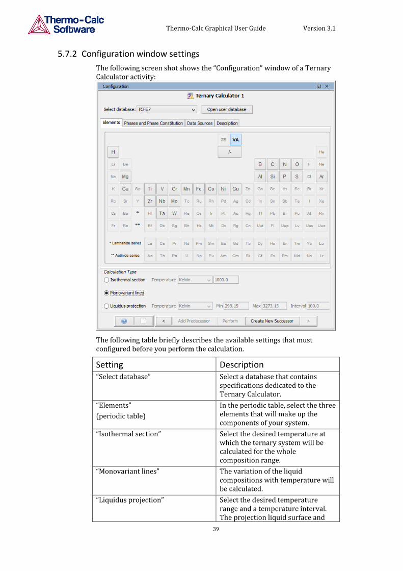
5.7.2 Configuration window settings
The following screen shot shows the “Configuration” window of a Ternary Calculator activity:
The following table briefly describes the available settings that must configured before you perform the calculation.
Setting Description “Select database” Select a database that contains
specifications dedicated to the Ternary Calculator.
“Elements”
(periodic table)
In the periodic table, select the three elements that will make up the components of your system.
“Isothermal section” Select the desired temperature at which the ternary system will be calculated for the whole composition range.
“Monovariant lines” The variation of the liquid compositions with temperature will be calculated.
“Liquidus projection” Select the desired temperature range and a temperature interval. The projection liquid surface and
Thermo-Calc Graphical User Guide Version 3.1
40
the monovariant lines will be calculated over the given temperature range.
5.8 Scheil Calculator
The Scheil Calculator activity is used to perform simulations of so-called Scheil (Scheil-Gulliver) solidification processes. By default, a Scheil calculation will result in an estimation of the solidification range of an alloy. The calculation is based on the assumptions that the liquid phase is homogeneous at all times and that the diffusivity is zero in the solid. However, it is possible to disregard the latter assumption for selected components.
For an example of how a Scheil Calculator can be used in a project, see example 8 in the Thermo-Calc Graphical Examples Collection.
5.8.1 Predecessors and successors
Possible predecessors System Definer
Possible successors Plot Renderer
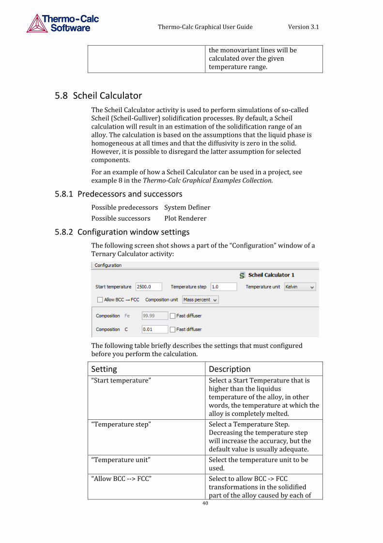
5.8.2 Configuration window settings
The following screen shot shows a part of the “Configuration” window of a Ternary Calculator activity:
The following table briefly describes the settings that must configured before you perform the calculation.
Setting Description “Start temperature” Select a Start Temperature that is
higher than the liquidus temperature of the alloy, in other words, the temperature at which the alloy is completely melted.
“Temperature step” Select a Temperature Step. Decreasing the temperature step will increase the accuracy, but the default value is usually adequate.
“Temperature unit” Select the temperature unit to be used.
“Allow BCC --> FCC” Select to allow BCC -> FCC transformations in the solidified part of the alloy caused by each of
Thermo-Calc Graphical User Guide Version 3.1
41
the components that you have specified to be “Fast Diffuser”. It is recommended that you only select this for steels.
“Composition unit” Select the composition unit to be used.
“Composition” Specify the composition of the alloy.
“Fast diffuser” Select if you want to allow redistribution of this component in both the solid and liquid parts of the alloy.