Release Notes: Thermo-Calc Software Package Version 2019bThermo-Calc version 2019b Thermo-Calc Version 2019b Highlights ★Thermo-Calc : T he new P rocess Metallurgy Module is designed

Release Notes:

Thermo-Calc Software Package

Version 2019b

© 2019 Foundation of Computational Thermodynamics: Solna, Sweden

Release notes Thermo-Calc version 2019b

Contents Thermo-Calc Version 2019b Release Highlights 4

Thermo-Calc 5

New Process Metallurgy Module 5

Process Metallurgy Calculator 5

License Requirements 6

Examples and Videos 6

New Template 6

Changed the Name of Two Calculation Types 6

One-Axis Plot Axes Quantities: Grouped and Flexible Modes 7

Gibbs Energy System (GES6) 7

GES6 vs GES5: Global and Local Settings 7

Change the Default Globally (Graphical and Console Mode) 7

Change the Version for a Local Session (Console Mode) 8

Defaults for the Software Development Kits (SDKs) 8

Note for Custom User Databases: Use the Database Checker for Verification 8

Logging Messages and Information 9

PARROT Optimization Users 9

Improvements, Changes and Bug Fixes 9

General 9

Graphical Mode Only 9

Project File Related 9

Plot Related 10

Speed Improvements 10

Both Graphical and Console Mode. TC-Python when indicated 10

Scheil Calculations 10

Keep Composition Set Numbers 11

Console Mode Only 11

Thermo-Calc Steel Model Library and Property Models 12

New Steel Library Template and Plotting Mode 12

New Template for the Steel Library - TTT Diagrams 12

New Plotting Option: TTT Mode 12

Improvements and Bug Fixes 13

Precipitation Module (TC-PRISMA) 13

New Growth Rate Models: NPLE and Para-equilibrium 13

1


New Example Using the Paraequilibrium Growth Rate Model 14


Diffusion Module (DICTRA) 15


Both Console and Graphical Mode 15

Graphical Mode Only (and TC-Python where Indicated) 16

Console Mode Only (and TC-Python where Indicated) 17

TC-Python API 18

New Features 18


Diffusion Improvements 18

Updating TC-Python from 2019a to 2019b 19

New TC-Python Examples 19

Diffusion 19

Miscellaneous 19

Databases 20

New Thermodynamic and Kinetic Databases 20

TCOX9 TCS Metal Oxide Solutions Database 20

Major changes from TCOX8 to TCOX9 20

TCCU3 TCS Cu-based Alloys Database 20

Major changes from TCCU2 to TCCU3 20

MOBCU3 TCS Cu Alloys Mobility Database 20

Changes from MOBCU2 to MOBCU3 20

Updated Thermodynamic and Kinetic Databases 21

TCFE9 TCS Steels/Fe-Alloys Database: Updated to version 9.1 21

Updates from TCFE9 to TCFE9.1 21

TCTI2 TCS Ti/TiAl-based Alloys Database: Updated to version 2.1 21

Updates from TCTI2 to TCTI2.1 21

Documentation, Examples and Tutorials 21

Reorganized Help and PDFs 21

New Tutorial: The Role of Diffusion in Materials 21

New Examples in Thermo-Calc 22

Precipitation Module (TC-PRISMA) Step-by-Step Instructions for Three Examples 22

Removed Console Mode Examples 22

TC-Python HTML Help on the Website 22

2


Installation 22

Thermo-Calc Changes and Improvements 22

Administrative Rights Needed for Windows Installation 22

Resources (e.g. manuals, materials folders) copied from Public to a User Documents folder (Windows only) 23

License File Installation Location 23

General 24

Linux installations 24

Demo and Academic Downloads and the new Process Metallurgy Module 24

TC-Python: New Script for Troubleshooting TC-Python Installations 24

Installation Disk Space Requirement 25

Platform Roadmap 25

3


Thermo-Calc Version 2019b

Highlights

★ Thermo-Calc: The new Process Metallurgy Module is designed for application to

steel-making and steel refining processes including converters, such as basic oxygen

furnaces, electric arc furnaces, ladle furnace metallurgy, and more. There is a new

version of the Gibbs Energy System calculation engine (GES6), a new easy-to-use

Steel Model Library template specifically for calculating TTT diagrams, some key

installation improvements, and a variety of other changes.

★ Precipitation Module (TC-PRISMA): Two new growth rate models are available for

use with the Precipitation Calculator: Para-equilibrium and Non-Partition Local

Equilibrium (NPLE). These models are designed specifically to address the fast

diffusion elements in Fe alloys. For details see Precipitation Module (TC-PRISMA).

★ Diffusion Module (DICTRA): Added several numerical options to be 'automatic' by

default. A simplified setup of homogenization simulations in Console Mode is also

implemented. See Diffusion Module (DICTRA). There is also a new comprehensive

tutorial available to teach you about the role of diffusion in materials. See

Documentation, Examples and Tutorials.

★ TC-Python: You can now set all options for each calculation type in a consistent way

using the with_option() method. There is also a method on the system object

that can convert between different composition units without performing an

equilibrium calculation, making the conversion much faster. For details about this

and other changes, see TC-Python API.

★ Databases: Three new database versions are available: TCOX9 TCS Metal Oxide

Solutions Database, TCCU3 TCS Cu-based Alloys Database, and MOBCU3 TCS Cu

Alloys Mobility Database. Two updated databases are also available: TCFE9 TCS

Steels/Fe-Alloys Database and TCTI2 TCS Ti/TiAl-based Alloys Database.

4


Thermo-Calc

New Process Metallurgy Module

The new Process Metallurgy Module includes the Process Metallurgy Calculator and makes it

easy to set up calculations for steel and slag. The new module is designed for application to

steel-making and steel refining processes including converters, such as basic oxygen furnaces,

electric arc furnaces, ladle furnace metallurgy, and more.

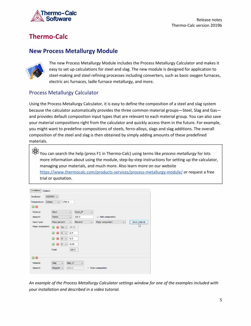
Process Metallurgy Calculator

Using the Process Metallurgy Calculator, it is easy to define the composition of a steel and slag system

because the calculator automatically provides the three common material groups—Steel, Slag and Gas—

and provides default composition input types that are relevant to each material group. You can also save

your material compositions right from the calculator and quickly access them in the future. For example,

you might want to predefine compositions of steels, ferro-alloys, slags and slag additions. The overall

composition of the steel and slag is then obtained by simply adding amounts of these predefined

materials.

You can search the help (press F1 in Thermo-Calc) using terms like process metallurgy for lots

more information about using the module, step-by-step instructions for setting up the calculator,

managing your materials, and much more. Also learn more on our website

https://www.thermocalc.com/products-services/process-metallurgy-module/ or request a free

trial or quotation.

An example of the Process Metallurgy Calculator settings window for one of the examples included with

your installation and described in a video tutorial.

5

https://www.thermocalc.com/products-services/process-metallurgy-module/


License Requirements

Users who have the thermodynamic database TCOX9 TCS Metal Oxide Solutions Database (which is also

new in this release) or the previous version, TCOX8, plus a valid Maintenance and Support Subscription

(M&SS) receive the new module for free. All other users can test the module with the included OXDEMO

database, which has been updated and includes the elements Al, C, Ca, Fe, O, S and Si.

Examples and Videos

Two examples plus companion videos are available to demonstrate some of the applications of the

Process Metallurgy Module. The project examples are available from in Thermo-Calc. Users with

Thermo-Calc 2019b who do not have TCOX8 or TCOX9 can still run the examples with the updated

OXDEMO database.

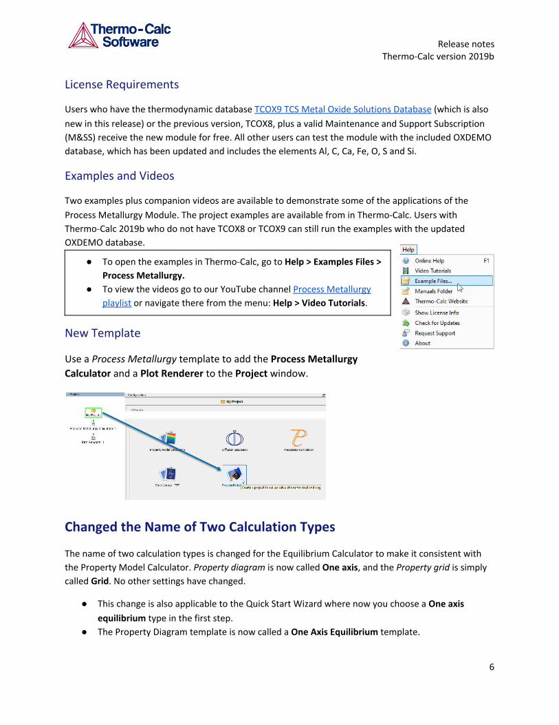
● To open the examples in Thermo-Calc, go to Help > Examples Files >

Process Metallurgy.

● To view the videos go to our YouTube channel Process Metallurgy

playlist or navigate there from the menu: Help > Video Tutorials.

New Template

Use a Process Metallurgy template to add the Process Metallurgy

Calculator and a Plot Renderer to the Project window.

Changed the Name of Two Calculation Types

The name of two calculation types is changed for the Equilibrium Calculator to make it consistent with

the Property Model Calculator. Property diagram is now called One axis, and the Property grid is simply

called Grid. No other settings have changed.

● This change is also applicable to the Quick Start Wizard where now you choose a One axis

equilibrium type in the first step.

● The Property Diagram template is now called a One Axis Equilibrium template.

6

https://www.youtube.com/playlist?list=PLfv6McToaTGS4g5LC9tjiqjCo9OX2-YOa

https://www.youtube.com/playlist?list=PLfv6McToaTGS4g5LC9tjiqjCo9OX2-YOa


One-Axis Plot Axes Quantities: Grouped and Flexible Modes

For the Equilibrium, Scheil, Binary, Ternary, Property Model, and Process Metallurgy Calculators, using a

One axis calculation type, the Grouped mode or Flexible mode is available on the Plot Renderer to help

you more easily define the plot quantities.

● Use Grouped mode to add and configure groups of axis quantities at the same time. For

example, change units or settings in groups with similar settings like temperature units or axis

types.

● Use Flexible mode to individually add and configure axes quantities and change the units or

other associated settings one at a time.

● There is also a new TTT mode available with the Property Model Calculator and the Steel Model

Library. See New Template for the Steel Library - TTT Diagrams and TTT Mode below.

Search the help for “One axis calculation”, or for “Grouped mode” or “Flexible mode”. The

settings are described for the Plot Renderer.

Gibbs Energy System (GES6)

The part of the calculation engine known as the Gibbs Energy System module, or GES for short, is

completely rewritten and is now updated from version 5 (GES5) to version 6 (GES6). GES6 is now

enabled by default.

The main purpose of GES6 is to support faster development of new features than is currently possible.

GES6 already shows improved calculation times for many long-running calculations. For short

calculations, the execution time of GES6 may be a little longer than for GES5.

Since GES6 does not yet support all the features of GES5, the two versions will continue to co-exist in the

application for some time to come. GES6 is enabled by default but in most cases it will fall back gracefully

to automatically use GES5 if a certain functionality is not yet implemented. When this is not possible you

will be advised by the application to manually switch to GES5.

GES6 vs GES5: Global and Local Settings

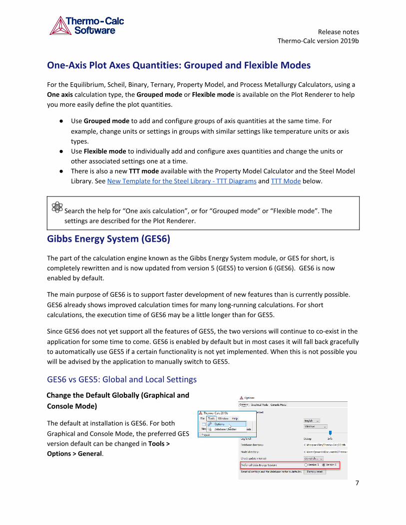
Change the Default Globally (Graphical and

Console Mode)

The default at installation is GES6. For both

Graphical and Console Mode, the preferred GES

version default can be changed in Tools >

Options > General.

7


● In Graphical Mode, the setting affects which GES version is used for all following calculations.

● In Console Mode, the setting affects which GES version is set as the default for newly launched

Console windows. The selected GES version of already existing Console window(s) is not

affected.

Change the Version for a Local Session (Console Mode)

In Console Mode, the preferred GES version can also be set with the SYS command SET_GES_VERSION. This setting is only applicable for the Console window in which the command is entered. If you launch a

new Console window it will always start with the default setting selected under Tools > Options >

General.

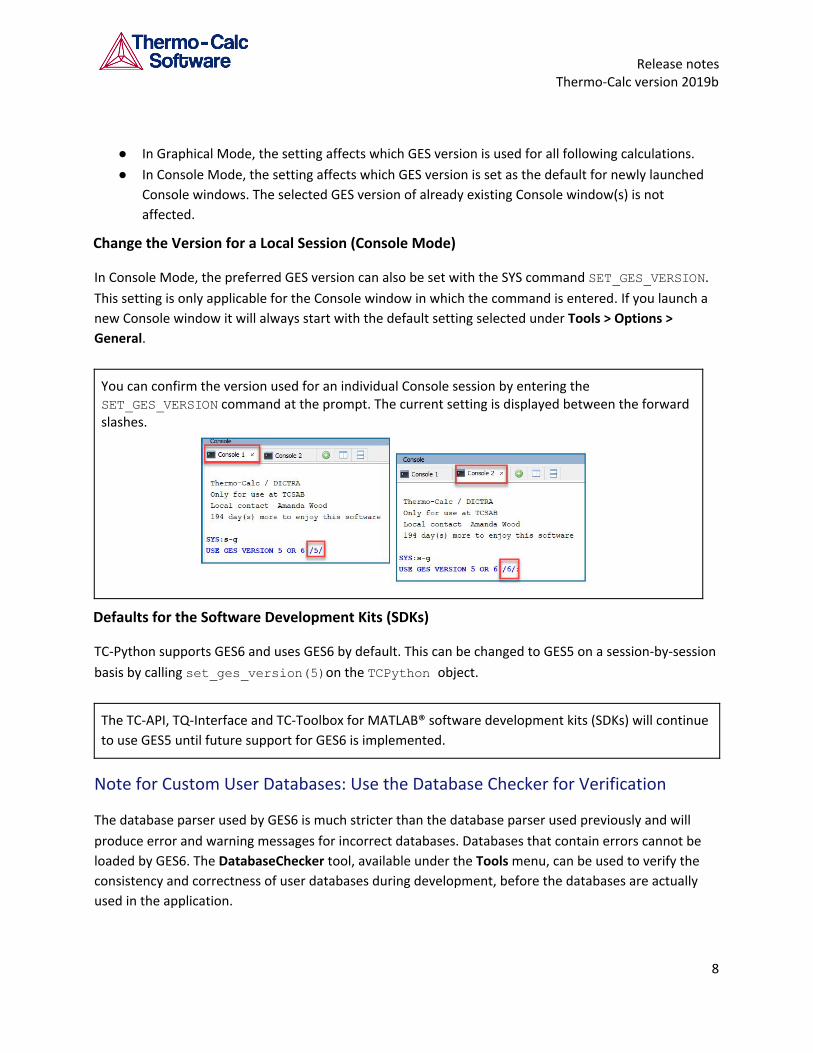
You can confirm the version used for an individual Console session by entering the SET_GES_VERSION command at the prompt. The current setting is displayed between the forward slashes.

Defaults for the Software Development Kits (SDKs)

TC-Python supports GES6 and uses GES6 by default. This can be changed to GES5 on a session-by-session

basis by calling set_ges_version(5)on the TCPython object.

The TC-API, TQ-Interface and TC-Toolbox for MATLAB® software development kits (SDKs) will continue

to use GES5 until future support for GES6 is implemented.

Note for Custom User Databases: Use the Database Checker for Verification

The database parser used by GES6 is much stricter than the database parser used previously and will

produce error and warning messages for incorrect databases. Databases that contain errors cannot be

loaded by GES6. The DatabaseChecker tool, available under the Tools menu, can be used to verify the

consistency and correctness of user databases during development, before the databases are actually

used in the application.

8


Logging Messages and Information

The use of GES6 is indicated in the log by the message “*** Invoking Gibbs Energy System v6 ***” and messages similar to “Verified the system state for 1 database(s) in 29 ms”. This may happen once, several times or not at all, depending on the compatibility of the calculations and

the database(s) with GES6 and how the Thermo-Calc application’s scheduler distributes the tasks of a

calculation. Otherwise, the use of GES6 will mostly be transparent.

PARROT Optimization Users

For PARROT optimization users, you need to use GES5. When you try to enter the PARROT

module, you are instructed to switch to GES5 using the SET_GES_VERSION command. To change

the default to use GES5, see Change the Default Globally (Graphical and Console Mode).

Improvements, Changes and Bug Fixes

General

● The Thermo-Calc temporary directory that was previously created to run subprocesses (e.g.

during a precipitation calculation) is now deleted afterwards.

● Apply Auto Layout: You can now reset the nodes in the Project window to the default layout. In

the Project window, right-click anywhere and choose Apply Auto Layout from the menu. The

nodes and the tree default to the center of the window.

Graphical Mode Only

Project File Related

● Stopped supporting old project files from Thermo-Calc version 4.1 and earlier. Starting from this

release, version 2019b, it is no longer possible to open project files created with version 4.1 or

older.

● Fixed a bug related to project files and when working between different platforms. When results

were saved in one platform (e.g. Windows) the project file would not open in the other platform

(e.g. Mac). Now if you switch platforms, the project file will open but then you have to re-run the

project file to get the results again.

● Improved how opening a project file works when you do not have a license for a database.

● Fixed a bug for the Equilibrium Calculator on the Options tab. Now the checkbox Control step size

is selected when the property is set in the Project file.

9


Plot Related

● Fixed a bug where choosing to turn off the legend would also hide the contour plot annotations.

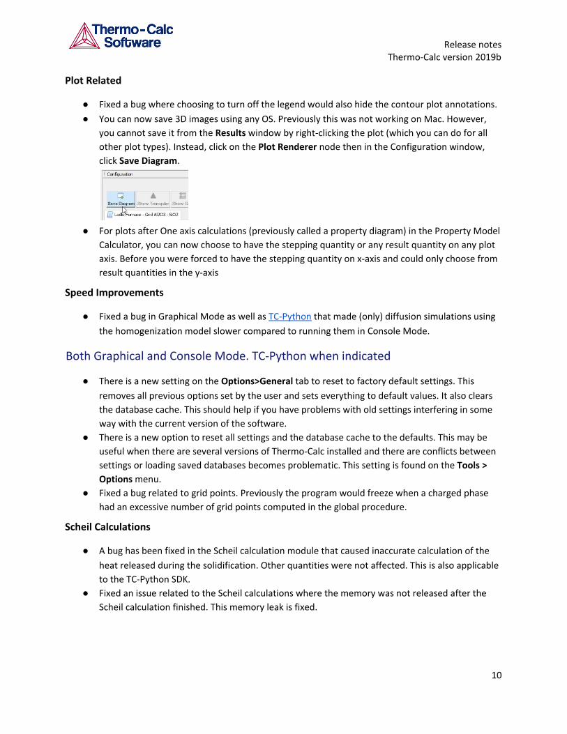
● You can now save 3D images using any OS. Previously this was not working on Mac. However,

you cannot save it from the Results window by right-clicking the plot (which you can do for all

other plot types). Instead, click on the Plot Renderer node then in the Configuration window,

click Save Diagram.

● For plots after One axis calculations (previously called a property diagram) in the Property Model

Calculator, you can now choose to have the stepping quantity or any result quantity on any plot

axis. Before you were forced to have the stepping quantity on x-axis and could only choose from

result quantities in the y-axis

Speed Improvements

● Fixed a bug in Graphical Mode as well as TC-Python that made (only) diffusion simulations using

the homogenization model slower compared to running them in Console Mode.

Both Graphical and Console Mode. TC-Python when indicated

● There is a new setting on the Options>General tab to reset to factory default settings. This

removes all previous options set by the user and sets everything to default values. It also clears

the database cache. This should help if you have problems with old settings interfering in some

way with the current version of the software.

● There is a new option to reset all settings and the database cache to the defaults. This may be

useful when there are several versions of Thermo-Calc installed and there are conflicts between

settings or loading saved databases becomes problematic. This setting is found on the Tools >

Options menu.

● Fixed a bug related to grid points. Previously the program would freeze when a charged phase

had an excessive number of grid points computed in the global procedure.

Scheil Calculations

● A bug has been fixed in the Scheil calculation module that caused inaccurate calculation of the

heat released during the solidification. Other quantities were not affected. This is also applicable

to the TC-Python SDK.

● Fixed an issue related to the Scheil calculations where the memory was not released after the

Scheil calculation finished. This memory leak is fixed.

10


Keep Composition Set Numbers

The composition set numbers from previous equilibrium calculations are now kept when the constitution

of a phase in the new equilibrium result is similar to the constitution of one of the composition sets of

that phase in the previous result. The major constituents, given in the thermodynamic database, are

used if no previous result exists.

By default the setting is ON within Thermo-Calc, and it affects all subsequent equilibrium calculations

until explicitly turned off again. When working in Graphical Mode, there is no option to turn this off,

whereas the setting can be turned on and off in Console Mode and it is available with all SDKs.

If this setting is on, performing the COMPUTE_EQUILIBRIUM command keeps the composition set

number for any phases that were also present in the last result from COMPUTE_EQUILIBRIUM.

The specific calculations where this is applicable is as follows.

● When in Console Mode and using the POLY3 module command COMPUTE_EQUILIBRIUM, this is

ON by default. To turn it off, go to ADVANCED OPTIONS and use a new command called

KEEP_COMP_SET_NUMBERS.

● If you are working with routines using the TQ-Interface this is OFF by default there and you use

the subroutine called TQKEEP_CS_NUMBERS (in Fortran), or tq_keep_cs_numbers (in C) to turn

it ON or OFF.

● When working with any of the other SDKs this can be turned ON and OFF again by using their

respective functions to run a POLY command.

● In Graphical Mode, for information only as the setting cannot be changed, this is set to ON in the

following calculation types: Equilibrium Calculator (Single equilibrium and Grid); Property Model

Calculator (in the general model "Equilibrium"), and for the Process Metallurgy Calculator (all

calculation types).

Console Mode Only

● Fixed a bug in the Gibbs Energy System (GES) module in Console Mode where you could not

enter a parameter when it had an asterisk * in a sub-lattice. It only worked when the * was in

the first sub-lattice, for example, G(FCC_L12,AL:*:VA;0) did not work.

● Fixed a bug that caused an exception when saving a plot image with a z-axis.

● Fixed a bug that could cause writing calculation results to file using the command TABULATE to

fail when the number of columns was large.

11


Thermo-Calc Steel Model Library and Property Models

Search the help (press F1 in Thermo-Calc) for more information about the Steel Model Library as

well as for details about the new template and TTT mode.

Use of the Steel Model Library (including the pearlite and martensite property models), the new steel TTT

template and TTT mode all require a valid Maintenance and Support Subscription (M&SS) plus licenses for

both the TCFE9 and MOBFE4 databases.

New Steel Library Template and Plotting Mode

New Template for the Steel Library - TTT Diagrams

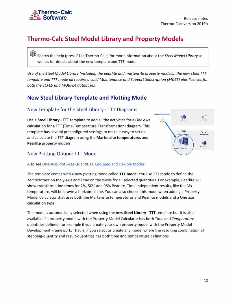
Use a Steel Library - TTT template to add all the activities for a One axis

calculation for a TTT (Time-Temperature-Transformation) diagram. This

template has several preconfigured settings to make it easy to set up

and calculate the TTT diagram using the Martensite temperatures and

Pearlite property models.

New Plotting Option: TTT Mode

Also see One-Axis Plot Axes Quantities: Grouped and Flexible Modes.

The template comes with a new plotting mode called TTT mode. You use TTT mode to define the

Temperature on the y-axis and Time on the x-axis for all selected quantities. For example, Pearlite will

show transformation times for 2%, 50% and 98% Pearlite. Time independent results, like the Ms

temperature, will be drawn a horizontal line. You can also choose this mode when adding a Property

Model Calculator that uses both the Martensite temperatures and Pearlite models and a One axis

calculation type.

The mode is automatically selected when using the new Steel Library - TTT template but it is also

available if a property model with the Property Model Calculator has both Time and Temperature

quantities defined, for example if you create your own property model with the Property Model

Development Framework. That is, if you select or create any model where the resulting combination of

stepping-quantity and result-quantities has both time and temperature definitions.

12


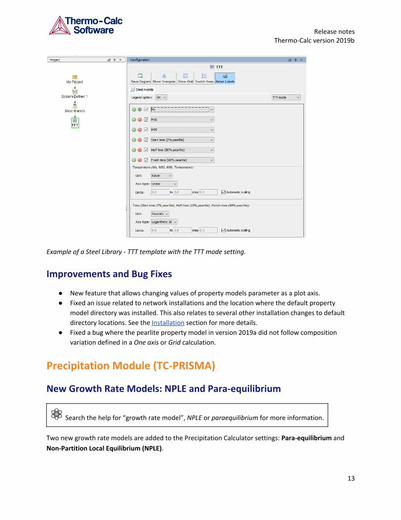
Example of a Steel Library - TTT template with the TTT mode setting.

Improvements and Bug Fixes

● New feature that allows changing values of property models parameter as a plot axis.

● Fixed an issue related to network installations and the location where the default property

model directory was installed. This also relates to several other installation changes to default

directory locations. See the Installation section for more details.

● Fixed a bug where the pearlite property model in version 2019a did not follow composition

variation defined in a One axis or Grid calculation.

Precipitation Module (TC-PRISMA)

New Growth Rate Models: NPLE and Para-equilibrium

Search the help for “growth rate model”, NPLE or paraequilibrium for more information.

Two new growth rate models are added to the Precipitation Calculator settings: Para-equilibrium and

Non-Partition Local Equilibrium (NPLE).

13


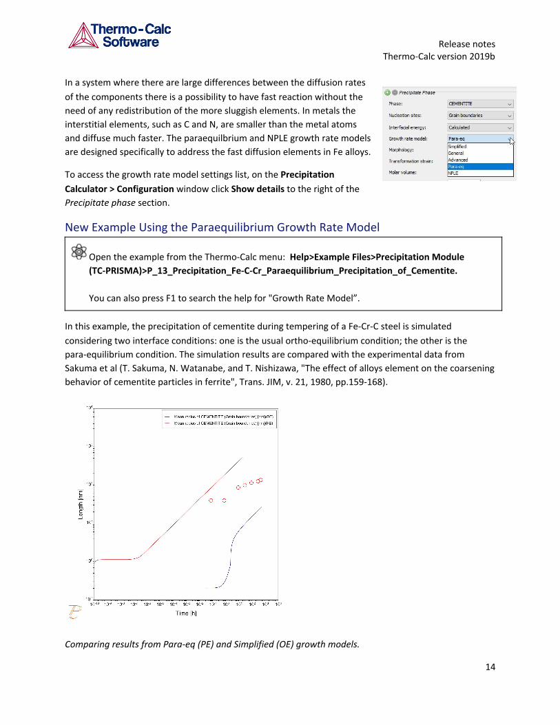
In a system where there are large differences between the diffusion rates

of the components there is a possibility to have fast reaction without the

need of any redistribution of the more sluggish elements. In metals the

interstitial elements, such as C and N, are smaller than the metal atoms

and diffuse much faster. The paraequilbrium and NPLE growth rate models

are designed specifically to address the fast diffusion elements in Fe alloys.

To access the growth rate model settings list, on the Precipitation

Calculator > Configuration window click Show details to the right of the

Precipitate phase section.

New Example Using the Paraequilibrium Growth Rate Model

Open the example from the Thermo-Calc menu: Help>Example Files>Precipitation Module

(TC-PRISMA)>P_13_Precipitation_Fe-C-Cr_Paraequilibrium_Precipitation_of_Cementite.

You can also press F1 to search the help for "Growth Rate Model”.

In this example, the precipitation of cementite during tempering of a Fe-Cr-C steel is simulated

considering two interface conditions: one is the usual ortho-equilibrium condition; the other is the

para-equilibrium condition. The simulation results are compared with the experimental data from

Sakuma et al (T. Sakuma, N. Watanabe, and T. Nishizawa, "The effect of alloys element on the coarsening

behavior of cementite particles in ferrite", Trans. JIM, v. 21, 1980, pp.159-168).

Comparing results from Para-eq (PE) and Simplified (OE) growth models.

14



● Fixed a bug for non-isothermal simulations with the Precipitation Calculator where the

simulation got stuck at the final time if nothing precipitated during the simulation. This is also

applicable to the TC-Python SDK.

● Fixed a bug from 2019a related to plotting results after a TTT or CCT calculation. You can now

change the temperature units on the Y-axis (e.g. from Kelvin to Celsius or vice versa).

Diffusion Module (DICTRA)


Both Console and Graphical Mode

● The labels for time and distance plot variables are now corrected and improved. There was a bug

for both Console and Graphical Mode where the output label was not correct.

● Fixed a bug related to the evaluation of some homogenization functions, for example using the

command ENTER_HOMOGENIZATION_FUNCTION. The affected homogenization functions are

Hashin-Shtrikman prescribed matrix phase, Hashin-Shtrikman prescribed matrix phase with

excluded phases, Hashin-Shtrikman majority phase as matrix phase and Hashin-Shtrikman

majority phase as matrix phase with excluded phases. ● “Automatic" options are implemented for the following settings in Graphical Mode> Diffusion

Calculator>Options and for the Console Mode command SET_SIMULATION_CONDITION: ○ Time integration method (Graphical Mode) and Degree of implicity when integrating

PDEs (Console Mode). With the automatic option, the default degree of implicity

correspond to trapezoidal (0.5) for classic and Euler Backward (1.0) for homogenization

model.

○ Use forced starting values in equilibrium calculations (Graphical Mode). When a phase

with an ordering contribution is entered into the simulation, for example the

gamma-prime/fcc_l12 phase in Ni-base superalloys, forced starting values are

automatically turned on.

○ The timestep is to be controlled by the phase interface displacement during the

simulation (Graphical Mode) and Check interface position (Console Mode). When a liquid

phase is entered in a simulation this option is automatically turned on.

15


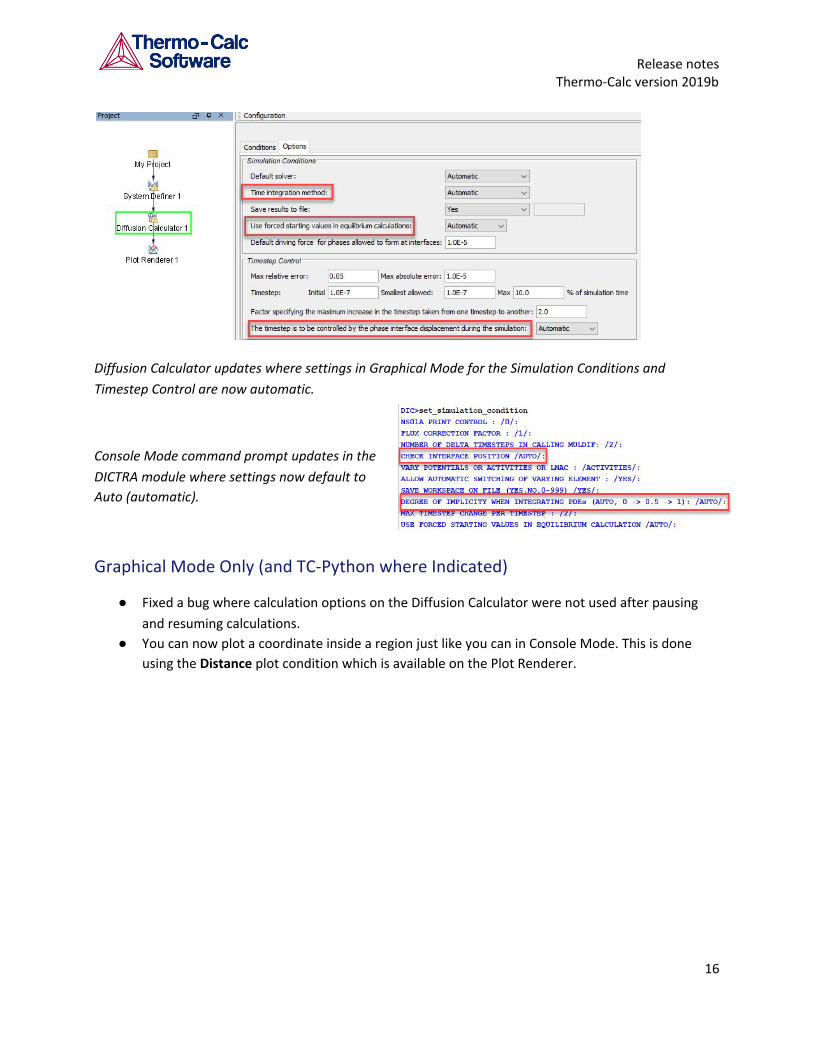
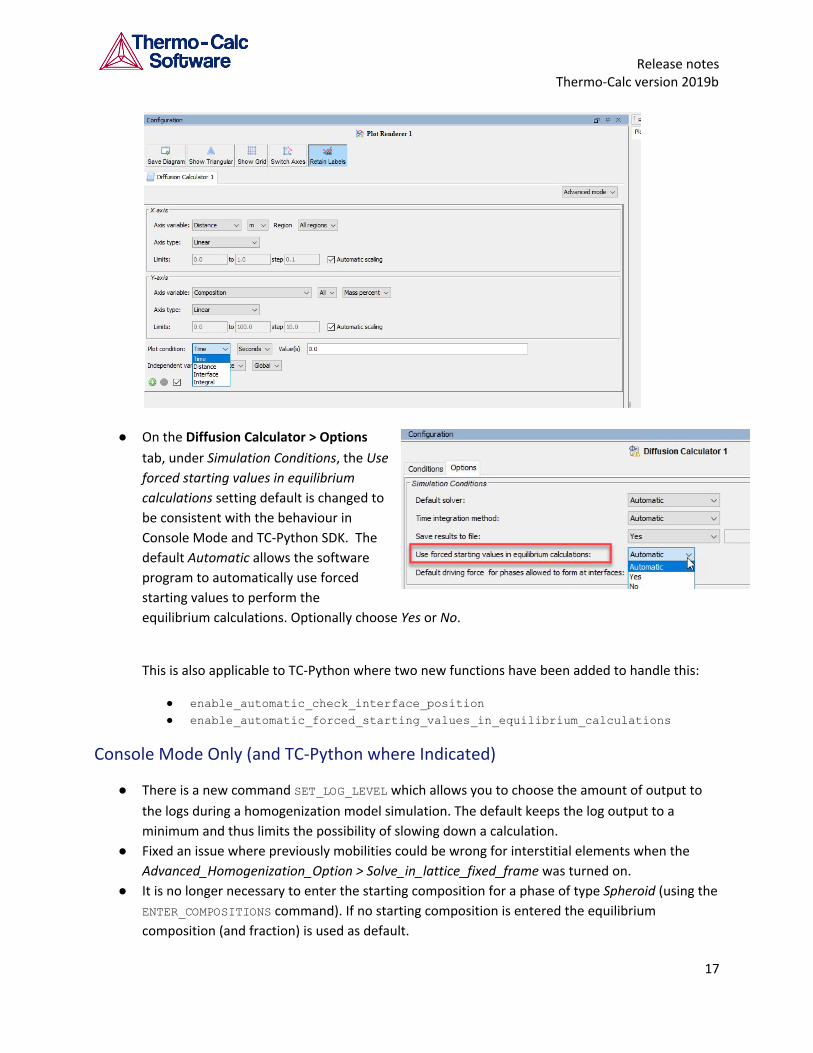
Diffusion Calculator updates where settings in Graphical Mode for the Simulation Conditions and

Timestep Control are now automatic.

Console Mode command prompt updates in the

DICTRA module where settings now default to

Auto (automatic).

Graphical Mode Only (and TC-Python where Indicated)

● Fixed a bug where calculation options on the Diffusion Calculator were not used after pausing

and resuming calculations.

● You can now plot a coordinate inside a region just like you can in Console Mode. This is done

using the Distance plot condition which is available on the Plot Renderer.

16


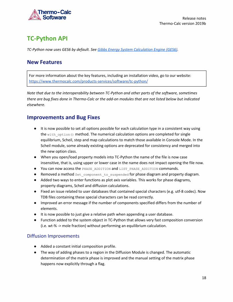
● On the Diffusion Calculator > Options

tab, under Simulation Conditions, the Use

forced starting values in equilibrium

calculations setting default is changed to

be consistent with the behaviour in

Console Mode and TC-Python SDK. The

default Automatic allows the software

program to automatically use forced

starting values to perform the

equilibrium calculations. Optionally choose Yes or No.

This is also applicable to TC-Python where two new functions have been added to handle this:

● enable_automatic_check_interface_position

● enable_automatic_forced_starting_values_in_equilibrium_calculations

Console Mode Only (and TC-Python where Indicated)

● There is a new command SET_LOG_LEVEL which allows you to choose the amount of output to

the logs during a homogenization model simulation. The default keeps the log output to a

minimum and thus limits the possibility of slowing down a calculation.

● Fixed an issue where previously mobilities could be wrong for interstitial elements when the

Advanced_Homogenization_Option > Solve_in_lattice_fixed_frame was turned on.

● It is no longer necessary to enter the starting composition for a phase of type Spheroid (using the

ENTER_COMPOSITIONS command). If no starting composition is entered the equilibrium

composition (and fraction) is used as default.

17


TC-Python API

TC-Python now uses GES6 by default. See Gibbs Energy System Calculation Engine (GES6).

New Features

For more information about the key features, including an installation video, go to our website:

https://www.thermocalc.com/products-services/software/tc-python/

Note that due to the interoperability between TC-Python and other parts of the software, sometimes

there are bug fixes done in Thermo-Calc or the add-on modules that are not listed below but indicated

elsewhere.


● It is now possible to set all options possible for each calculation type in a consistent way using

the with_option() method. The numerical calculation options are completed for single

equilibrium, Scheil, step and map calculations to match those available in Console Mode. In the

Scheil module, some already existing options are deprecated for consistency and merged into

the new option class.

● When you open/load property models into TC-Python the name of the file is now case

insensitive, that is, using upper or lower case in the name does not impact opening the file now.

● You can now access the PHASE_ADDITION and LIST_PHASE_ADDITION commands. ● Removed a method Set_component_to_suspended for phase diagram and property diagram.

● Added two ways to enter functions as plot axis variables. This works for phase diagrams,

property diagrams, Scheil and diffusion calculations.

● Fixed an issue related to user databases that contained special characters (e.g. utf-8 codec). Now

TDB files containing these special characters can be read correctly.

● Improved an error message if the number of components specified differs from the number of

elements.

● It is now possible to just give a relative path when appending a user database.

● Function added to the system object in TC-Python that allows very fast composition conversion

(i.e. wt-% -> mole fraction) without performing an equilibrium calculation.

Diffusion Improvements

● Added a constant initial composition profile.

● The way of adding phases to a region in the Diffusion Module is changed. The automatic

determination of the matrix phase is improved and the manual setting of the matrix phase

happens now explicitly through a flag.

18

https://www.thermocalc.com/products-services/software/tc-python/


● A bug was fixed in TC-Python that prevented the calculation cache from working correctly for

diffusion calculations with multiple phases in one region.

● The syntax of the diffusion quantity constructors DistanceCondition / PlotCondition.distance() and TimeCondition / PlotCondition.time() is changed due

to necessary bug fixes.

Updating TC-Python from 2019a to 2019b

Note the following if you installed earlier versions of TC-Python with Thermo-Calc. When updating to a

newer version of Thermo-Calc, you always also need to install the latest version of TC-Python. It is not

sufficient to run the installer of Thermo-Calc. See the section “Updating to a newer version” in the

TC-Python Quick Installation Guide. You can also search the help in Thermo-Calc or open the HTML

version of the TC-Python help available on our website (which is also included with your installation).

New TC-Python Examples

Diffusion

There is a new diffusion example called pyex_D_07_Homogenization_Of_Scheil_Profile.py. It demonstrates the simulation of the homogenization heat treatment of an alloy from the as-cast state. As

a first step, the microsegregation after solidification is simulated using a Scheil-calculation, then as a

second step the homogenization is simulated using a diffusion simulation.

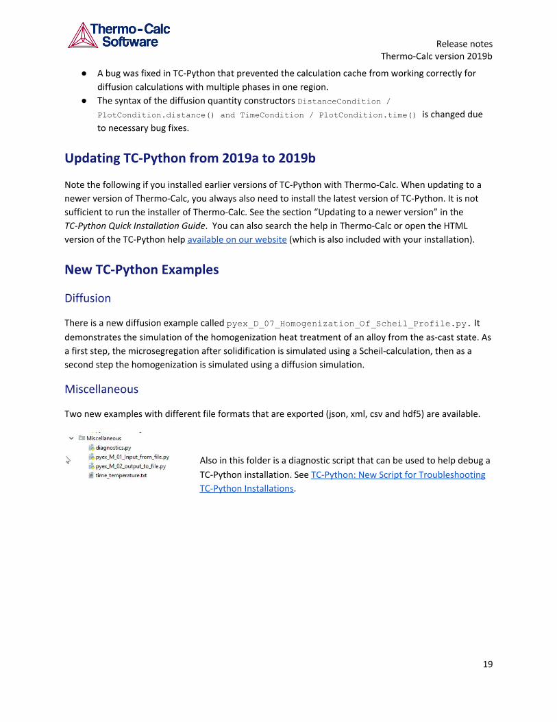
Miscellaneous

Two new examples with different file formats that are exported (json, xml, csv and hdf5) are available.

Also in this folder is a diagnostic script that can be used to help debug a

TC-Python installation. See TC-Python: New Script for Troubleshooting

TC-Python Installations.

19

https://www2.thermocalc.com/downloads/support/python/python/index.html


Databases

New Thermodynamic and Kinetic Databases

TCOX9 TCS Metal Oxide Solutions Database

Major changes from TCOX8 to TCOX9

● Addition of Ti: Assessed or added from literature all binary and a few ternary metallic systems.

Assessed Ti-O and Ti-S binary systems. Assessed 19 ternary Me-Ti-O, 2 Me-Ti-S and 23 higher

order oxide systems as indicated in the TCOX information sheet. Ti+2/+3/+4 is included in the

liquid oxide, so the correct distribution of oxidation states in the slag can be calculated.

● The following systems have been assessed for version 9: CaO-SiO2-VOx. The correct distribution

of oxidation states in the slag (+3/+4/+5) can now be calculated.

● The following systems have been reassessed for version 9: Ca-O-V, Mg-O-V, O-Si-V and and

CaO-SiO2-Y2O3. ● The following systems have been estimated for version 9: MgO-SiO2-VOx, MnS-NbS, MnS-VS.

● Changed model for VO solid solution, from Halite to FCC_A1 to be consistent with cubic TiO.

Reassessed solubility of V2O3 in CaO/CoO/FeO/MgO/MnO/NiO Halite due to change of model for

VO. Assessed C-V-O, modeling complete solid solution between VCx and VOy (same applies to the

C-Ti-O system).

● Merged CoV2O6 and NiV2O6 compounds to the CaV2O6 phase.

● Removed the SO4-2 species in the liquid phase.

● Minor changes to the following systems: W-O, Al-Cr-O, Ca-Ni-O, Co-O-V, Cr-Cu-O, Mg-Mn-O,

Co-Mn-O, Co-Mo-O, Co-O-P, Nb-O-P, Ni-O-Si, Ni-O-V, Al-Ca-Ni-O, Al-Ni-O-Y, Ca-Co-Cu-O,

Ca-Co-Ni-O, Co-Mn-O-Y, Fe-La-Ni-O, Gd-Mn-O-Si.

TCCU3 TCS Cu-based Alloys Database

Major changes from TCCU2 to TCCU3

● Addition of Ge.

● 10 Ge-X (X=Ag, Al, Au, Co, Cr, Cu, Ni, Sn, Ti, Zr) binary systems are added.

● 2 ternary systems Ag-Cu-Ge and Au-Cu-Ge are included.

● Volume data for the newly added phases are assessed or estimated.

MOBCU3 TCS Cu Alloys Mobility Database

Changes from MOBCU2 to MOBCU3

This database is compatible with TCS Cu-based Alloys Database (TCCU3) and the update from MOBCU2

to MOBCU3 now contains data for the diffusion of the new element Ge in both Fcc and liquid phases of

Cu alloys.

20


Updated Thermodynamic and Kinetic Databases

TCFE9 TCS Steels/Fe-Alloys Database: Updated to version 9.1

Updates from TCFE9 to TCFE9.1

● Revision of C-Fe-S system.

● Revision of Cr-Fe-Nb and Fe-Nb-Si system and the addition of 15 new silicide phases.

● Revision of the Laves phase description in Fe-Nb-W and Cr-Mo-Nb systems.

● Updates to the molar volumes of Liquid Mn, CEMENTITE, Fe-Si-B ternary phases, MNS, and

several sulfides.

● Correction of the magnetic properties of CBCC_A12 phase.

● Removing the pressure dependent parameters from Fe for compatibility with GES6.

TCTI2 TCS Ti/TiAl-based Alloys Database: Updated to version 2.1

Updates from TCTI2 to TCTI2.1

● Improved description of liquidus temperature for Ti64 alloy.

● Adjusted phase stability of HCP_A3 and BCC_A2 in some systems.

Documentation, Examples and Tutorials

Reorganized Help and PDFs

The online help (and therefore the PDF documentation) is updated and reorganized to better reflect the

divergence between the Graphical Mode and Console Mode content. The help is continuously being

improved and streamlined but if you find any issues or want to contribute to the content, send an email

to [email protected].

New Tutorial: The Role of Diffusion in Materials

A new set of examples is available. This comprehensive tutorial teaches you about the role of diffusion in

materials and how the Diffusion Module (DICTRA) can be applied to materials design and processing.

The tutorial is intended for engineers interested in using the Diffusion Module (DICTRA), as well as

students learning about the role of diffusion in materials. It is designed to be useful at many levels, from

undergraduate studies to someone with a PhD and experience in a related field. Fill out a short form on

our website to access The Role of Diffusion in Materials tutorial.

21

https://www.thermocalc.com/products-services/software/diffusion-module-(dictra)/the-role-of-diffusion-in-materials-tutorial/


New Examples in Thermo-Calc

There are new examples described elsewhere in this document:

● TC-Python: See TC-Python API. ● Precipitation Module (TC-PRISMA): New paraequilibrium growth rate model. See the

Precipitation Module (TC-PRISMA) section for details. Also see Precipitation Module (TC-PRISMA)

Step-by-Step Instructions for Three Examples. ● Process Metallurgy: See New Process Metallurgy Module.

Precipitation Module (TC-PRISMA) Step-by-Step Instructions for Three

Examples

The following examples now have a PDF that includes step-by-step instructions about how to recreate

the project file included with your installation:

● P_01: Isothermal Precipitation of Al3Sc

● P_07: Continuous Cooling Transformation (CCT) Diagram of Ni-Al-Cr γ-γ’

● P_09: Precipitation of Al-Sc AL3SC with Assumption of Sphere and Cuboid Morphologies

You can access the PDF from within Thermo-Calc help.

Removed Console Mode Examples

Thermo-Calc examples tcex-45, tcex-46 and tcex-47 have been removed from the Console Mode

Example collection as 3D plots in Console Mode rely on external third-party tools no longer available.

TC-Python HTML Help on the Website

The HTML version of the TC-Python help is now available on our website as well as included with your

installation.

Installation

Thermo-Calc Changes and Improvements

Administrative Rights Needed for Windows Installation

Windows installations now require administrator rights to install and

uninstall the program.

22

https://www2.thermocalc.com/downloads/support/python/python/index.html


Resources (e.g. manuals, materials folders) copied from Public to a User

Documents folder (Windows only)

This is for Windows operating systems. Note that access to some of the folder contents shown requires

additional licenses.

The default folders where documents, materials files, property models and other content is installed

under Public Documents for ALL USERS. For a local user these files are copied to the user’s Documents

folder where this local copy is associated to the user login. The Public Documents folder will always

contain the original set of contents as per the installation.

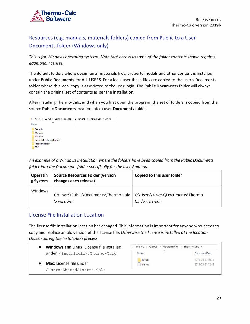
After installing Thermo-Calc, and when you first open the program, the set of folders is copied from the

source Public Documents location into a user Documents folder.

An example of a Windows installation where the folders have been copied from the Public Documents

folder into the Documents folder specifically for the user Amanda.

Operating System

Source Resources Folder (version changes each release)

Copied to this user folder

Windows C:\Users\Public\Documents\Thermo-Calc

\<version>

C:\Users\<user>\Documents\Thermo-

Calc\<version>

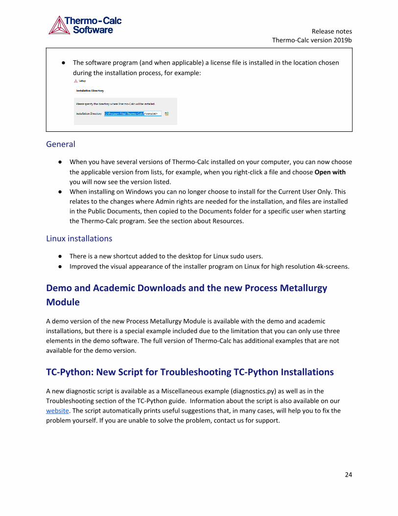
License File Installation Location

The license file installation location has changed. This information is important for anyone who needs to

copy and replace an old version of the license file. Otherwise the license is installed at the location

chosen during the installation process.

● Windows and Linux: License file installed

under <installdir>/Thermo-Calc

● Mac: License file under

/Users/Shared/Thermo-Calc

23


● The software program (and when applicable) a license file is installed in the location chosen

during the installation process, for example:

General

● When you have several versions of Thermo-Calc installed on your computer, you can now choose

the applicable version from lists, for example, when you right-click a file and choose Open with

you will now see the version listed.

● When installing on Windows you can no longer choose to install for the Current User Only. This

relates to the changes where Admin rights are needed for the installation, and files are installed

in the Public Documents, then copied to the Documents folder for a specific user when starting

the Thermo-Calc program. See the section about Resources.

Linux installations

● There is a new shortcut added to the desktop for Linux sudo users.

● Improved the visual appearance of the installer program on Linux for high resolution 4k-screens.

Demo and Academic Downloads and the new Process Metallurgy

Module

A demo version of the new Process Metallurgy Module is available with the demo and academic

installations, but there is a special example included due to the limitation that you can only use three

elements in the demo software. The full version of Thermo-Calc has additional examples that are not

available for the demo version.

TC-Python: New Script for Troubleshooting TC-Python Installations

A new diagnostic script is available as a Miscellaneous example (diagnostics.py) as well as in the

Troubleshooting section of the TC-Python guide. Information about the script is also available on our

website. The script automatically prints useful suggestions that, in many cases, will help you to fix the

problem yourself. If you are unable to solve the problem, contact us for support.

24

https://www.thermocalc.com/products-services/software/tc-python/#troubleshooting


Installation Disk Space Requirement

Due to precompiled databases added to the Thermo-Calc installation, 2 GB of disk space and 8 GB of

RAM is recommended for the 2019b installation.

Platform Roadmap

For information about platforms being phased out visit our website

http://www.thermocalc.com/products-services/software/system-requirements/platformroadmap/.

25

http://www.thermocalc.com/products-services/software/system-requirements/platformroadmap/