Release Notes: Thermo-Calc Software Package Version 2017b · Release Notes: Thermo-Calc Software Package . Version 2017b . Release notes Thermo-Calc version 2017b . 2 of 24| Contents

© 2017 Foundation of Computational Thermodynamics: Stockholm, Sweden

Release Notes:

Thermo-Calc Software Package

Version 2017b

Release notes Thermo-Calc version 2017b

2 of 24|

Contents Thermo-Calc 2017b ................................................................................................... 4 Databases ................................................................................................................. 5

TCTI1 TCS Ti/TiAl-based Alloys Thermodynamic Database ....................................................... 5 TCNOBL1 TCS Noble Metal-based Alloys Database ................................................................... 5

TCAL5 TCS Aluminium-based Alloys Database .......................................................................... 6 TCHEA version 2.1 TCS High Entropy Alloys Database .............................................................. 7 MOBTI2 TCS Ti-alloys Mobility Database .................................................................................. 7 SSUB6 SGTE Substances Database ............................................................................................ 7 New Copper Demo Databases ................................................................................................... 8

Thermo-Calc ............................................................................................................. 8

Windows OS ............................................................................................................................... 9 Linux and Mac OS .................................................................................................................... 10

General .................................................................................................................................... 10 Activity Nodes (e.g. System Definer and Calculators) (Graphical Mode) ................................ 11 Project Files (.tcu) (Graphical Mode) ....................................................................................... 11 Experimental Data (*.EXP) Files .............................................................................................. 11 Plots and Tables ....................................................................................................................... 12 DATAPLOT DIGLIB Symbols ...................................................................................................... 13 Scheil Calculations ................................................................................................................... 13 Batching Improvements .......................................................................................................... 14

Diffusion Module (DICTRA) ..................................................................................... 14

Boundary Conditions ............................................................................................................... 14 Table Renderer ........................................................................................................................ 15 Initial Composition Visualization ............................................................................................. 15 Advanced Mode in Plotting ..................................................................................................... 16

D_05 γ/α/γ Diffusion couple of Fe-Ni-Cr alloys ....................................................................... 17 D_06 Diffusion Through a Tube Wall ...................................................................................... 17 D_07 Multiphase Carburization of a Ni-25 Cr-0.0001C alloy .................................................. 17

USE_INTERPOLATION_FOR_D ................................................................................................. 17

Precipitation Module (TC-PRISMA).......................................................................... 19

P_07: Cooling Rate (CCT) Diagram of Ni-Al-Cr γ-γ’ .................................................................. 19

About the Cuboid, Plate and Needle Morphologies ................................................................ 20


3 of 24|

P_08: Precipitation of Cu-Ti CU4TI1 with Assumptions of Sphere and Needle Morphologies 21 P_09: Precipitation of Al-Sc AL3SC with Assumption of Sphere and Cuboid Morphologies .... 21

Documentation and Examples ................................................................................ 22

New Examples for the Add-on Modules .................................................................................. 22 New Names and Folders for the Graphical Mode Examples ................................................... 23 Property Model Development Framework Tutorial Examples ................................................ 23 DATAPLOT Examples ............................................................................................................... 23 TQ-Interface Examples ............................................................................................................ 24

New and Updated Training Videos .......................................................................... 24 Installation Disk Space Requirement ....................................................................... 24 Platform Roadmap ................................................................................................. 24


4 of 24|

Thermo-Calc 2017b Highlights

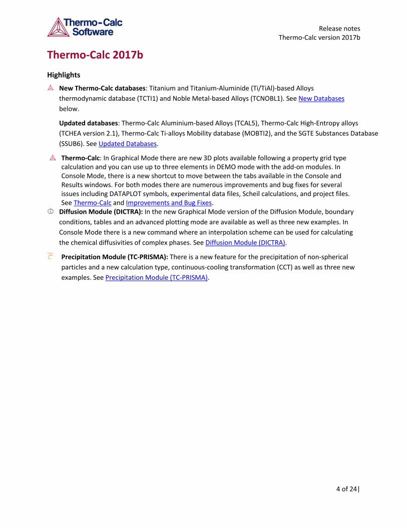
New Thermo-Calc databases: Titanium and Titanium-Aluminide (Ti/TiAl)-based Alloys thermodynamic database (TCTI1) and Noble Metal-based Alloys (TCNOBL1). See New Databases below.

Updated databases: Thermo-Calc Aluminium-based Alloys (TCAL5), Thermo-Calc High-Entropy alloys (TCHEA version 2.1), Thermo-Calc Ti-alloys Mobility database (MOBTI2), and the SGTE Substances Database (SSUB6). See Updated Databases.

Thermo-Calc: In Graphical Mode there are new 3D plots available following a property grid type calculation and you can use up to three elements in DEMO mode with the add-on modules. In Console Mode, there is a new shortcut to move between the tabs available in the Console and Results windows. For both modes there are numerous improvements and bug fixes for several issues including DATAPLOT symbols, experimental data files, Scheil calculations, and project files. See Thermo-Calc and Improvements and Bug Fixes.

Diffusion Module (DICTRA): In the new Graphical Mode version of the Diffusion Module, boundary conditions, tables and an advanced plotting mode are available as well as three new examples. In Console Mode there is a new command where an interpolation scheme can be used for calculating the chemical diffusivities of complex phases. See Diffusion Module (DICTRA).

Precipitation Module (TC-PRISMA): There is a new feature for the precipitation of non-spherical particles and a new calculation type, continuous-cooling transformation (CCT) as well as three new examples. See Precipitation Module (TC-PRISMA).


5 of 24|

Databases

New Databases

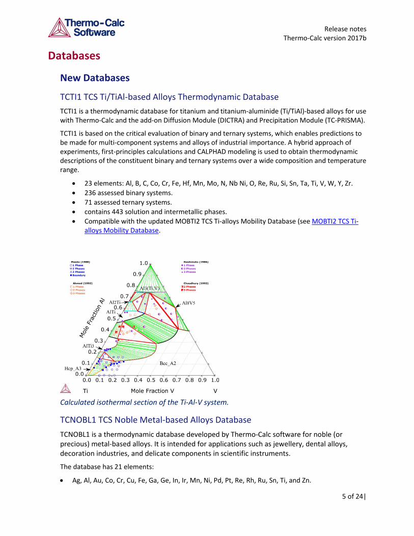
TCTI1 TCS Ti/TiAl-based Alloys Thermodynamic Database TCTI1 is a thermodynamic database for titanium and titanium-aluminide (Ti/TiAl)-based alloys for use with Thermo-Calc and the add-on Diffusion Module (DICTRA) and Precipitation Module (TC-PRISMA).

TCTI1 is based on the critical evaluation of binary and ternary systems, which enables predictions to be made for multi-component systems and alloys of industrial importance. A hybrid approach of experiments, first-principles calculations and CALPHAD modeling is used to obtain thermodynamic descriptions of the constituent binary and ternary systems over a wide composition and temperature range.

• 23 elements: Al, B, C, Co, Cr, Fe, Hf, Mn, Mo, N, Nb Ni, O, Re, Ru, Si, Sn, Ta, Ti, V, W, Y, Zr. • 236 assessed binary systems. • 71 assessed ternary systems. • contains 443 solution and intermetallic phases. • Compatible with the updated MOBTI2 TCS Ti-alloys Mobility Database (see MOBTI2 TCS Ti-

alloys Mobility Database.

Calculated isothermal section of the Ti-Al-V system.

TCNOBL1 TCS Noble Metal-based Alloys Database TCNOBL1 is a thermodynamic database developed by Thermo-Calc software for noble (or precious) metal-based alloys. It is intended for applications such as jewellery, dental alloys, decoration industries, and delicate components in scientific instruments.

The database has 21 elements:

• Ag, Al, Au, Co, Cr, Cu, Fe, Ga, Ge, In, Ir, Mn, Ni, Pd, Pt, Re, Rh, Ru, Sn, Ti, and Zn.


6 of 24|

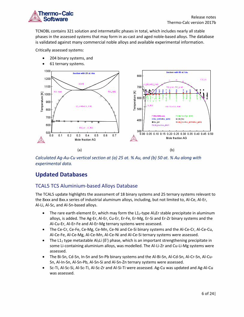
TCNOBL contains 321 solution and intermetallic phases in total, which includes nearly all stable phases in the assessed systems that may form in as-cast and aged noble-based alloys. The database is validated against many commercial noble alloys and available experimental information.

Critically assessed systems:

• 204 binary systems, and • 61 ternary systems.

(a) (b)

Calculated Ag-Au-Cu vertical section at (a) 25 at. % Au, and (b) 50 at. % Au along with experimental data.

Updated Databases

TCAL5 TCS Aluminium-based Alloys Database The TCAL5 update highlights the assessment of 18 binary systems and 25 ternary systems relevant to the 8xxx and 8xx.x series of industrial aluminum alloys, including, but not limited to, Al-Ce, Al-Er, Al-Li, Al-Sc, and Al-Sn-based alloys.

• The rare earth element Er, which may form the L12-type Al3Er stable precipitate in aluminum alloys, is added. The Ag-Er, Al-Er, Cu-Er, Er-Fe, Er-Mg, Er-Si and Er-Zr binary systems and the Al-Cu-Er, Al-Er-Fe and Al-Er-Mg ternary systems were assessed.

• The Ce-Cr, Ce-Fe, Ce-Mg, Ce-Mn, Ce-Ni and Ce-Si binary systems and the Al-Ce-Cr, Al-Ce-Cu, Al-Ce-Fe, Al-Ce-Mg, Al-Ce-Mn, Al-Ce-Ni and Al-Ce-Si ternary systems were assessed.

• The L12 type metastable Al3Li (δ') phase, which is an important strengthening precipitate in some Li-containing aluminium alloys, was modelled. The Al-Li-Zr and Cu-Li-Mg systems were assessed.

• The Bi-Sn, Cd-Sn, In-Sn and Sn-Pb binary systems and the Al-Bi-Sn, Al-Cd-Sn, Al-Cr-Sn, Al-Cu-Sn, Al-In-Sn, Al-Sn-Pb, Al-Sn-Si and Al-Sn-Zn ternary systems were assessed.

• Sc-Ti, Al-Sc-Si, Al-Sc-Ti, Al-Sc-Zr and Al-Si-Ti were assessed. Ag-Cu was updated and Ag-Al-Cu was assessed.


7 of 24|

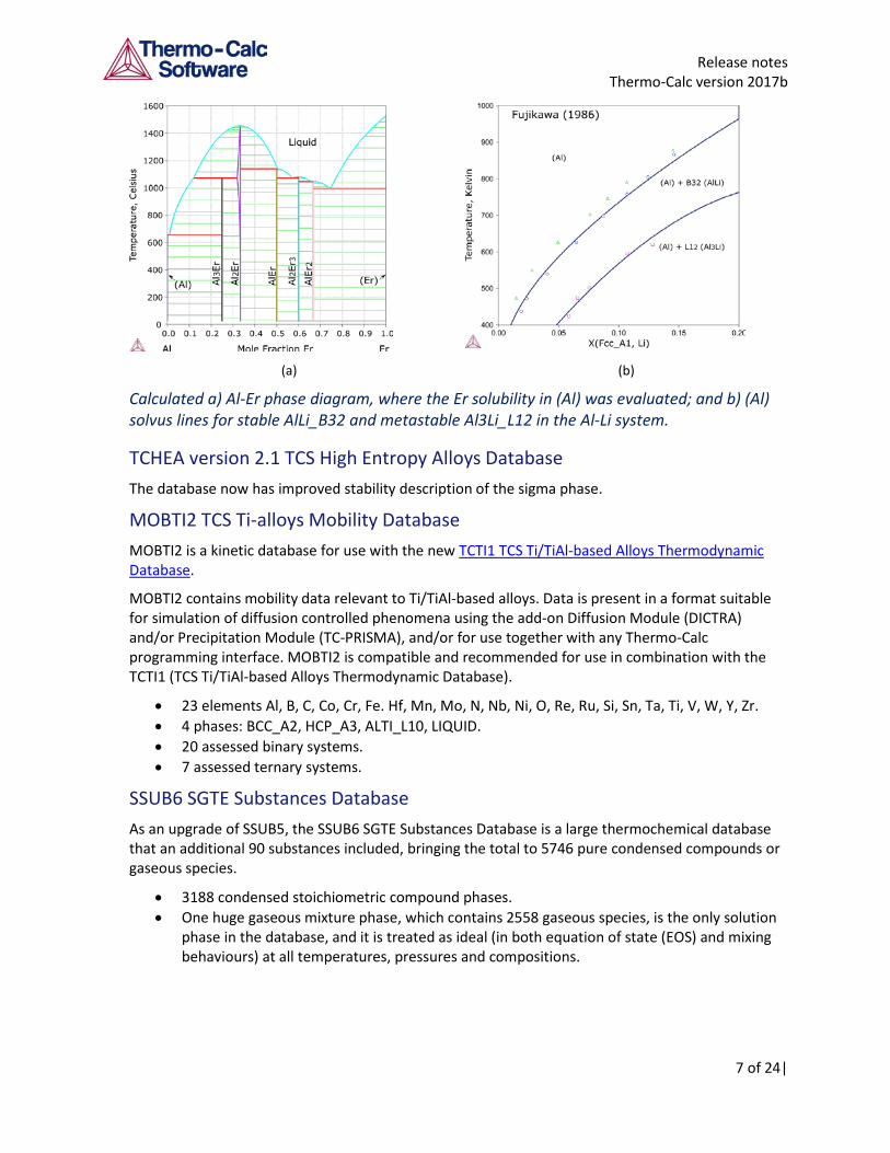
(a) (b)

Calculated a) Al-Er phase diagram, where the Er solubility in (Al) was evaluated; and b) (Al) solvus lines for stable AlLi_B32 and metastable Al3Li_L12 in the Al-Li system.

TCHEA version 2.1 TCS High Entropy Alloys Database The database now has improved stability description of the sigma phase.

MOBTI2 TCS Ti-alloys Mobility Database MOBTI2 is a kinetic database for use with the new TCTI1 TCS Ti/TiAl-based Alloys Thermodynamic Database.

MOBTI2 contains mobility data relevant to Ti/TiAl-based alloys. Data is present in a format suitable for simulation of diffusion controlled phenomena using the add-on Diffusion Module (DICTRA) and/or Precipitation Module (TC-PRISMA), and/or for use together with any Thermo-Calc programming interface. MOBTI2 is compatible and recommended for use in combination with the TCTI1 (TCS Ti/TiAl-based Alloys Thermodynamic Database).

• 23 elements Al, B, C, Co, Cr, Fe. Hf, Mn, Mo, N, Nb, Ni, O, Re, Ru, Si, Sn, Ta, Ti, V, W, Y, Zr. • 4 phases: BCC_A2, HCP_A3, ALTI_L10, LIQUID. • 20 assessed binary systems. • 7 assessed ternary systems.

SSUB6 SGTE Substances Database As an upgrade of SSUB5, the SSUB6 SGTE Substances Database is a large thermochemical database that an additional 90 substances included, bringing the total to 5746 pure condensed compounds or gaseous species.

• 3188 condensed stoichiometric compound phases. • One huge gaseous mixture phase, which contains 2558 gaseous species, is the only solution

phase in the database, and it is treated as ideal (in both equation of state (EOS) and mixing behaviours) at all temperatures, pressures and compositions.


8 of 24|

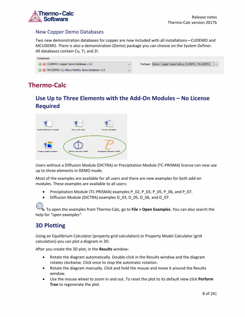
New Copper Demo Databases Two new demonstration databases for copper are now included with all installations—CUDEMO and MCUDEMO. There is also a demonstration (Demo) package you can choose on the System Definer. All databases contain Cu, Ti, and Zr.

Thermo-Calc

Use Up to Three Elements with the Add-On Modules – No License Required

Users without a Diffusion Module (DICTRA) or Precipitation Module (TC-PRISMA) license can now use up to three elements in DEMO mode.

Most of the examples are available for all users and there are new examples for both add-on modules. These examples are available to all users:

• Precipitation Module (TC-PRISMA) examples P_02, P_03, P_05, P_06, and P_07. • Diffusion Module (DICTRA) examples D_03, D_05, D_06, and D_07.

To open the examples from Thermo-Calc, go to File > Open Examples. You can also search the help for “open examples”.

3D Plotting Using an Equilibrium Calculator (property grid calculation) or Property Model Calculator (grid calculation) you can plot a diagram in 3D.

After you create the 3D plot, in the Results window:

• Rotate the diagram automatically. Double-click in the Results window and the diagram rotates clockwise. Click once to stop the automatic rotation.

• Rotate the diagram manually. Click and hold the mouse and move it around the Results window.

• Use the mouse wheel to zoom in and out. To reset the plot to its default view click Perform Tree to regenerate the plot.


9 of 24|

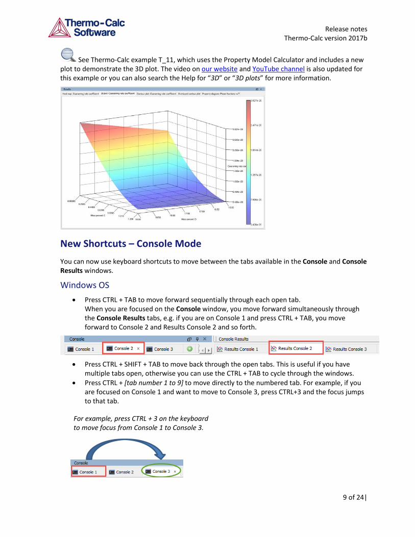
See Thermo-Calc example T_11, which uses the Property Model Calculator and includes a new plot to demonstrate the 3D plot. The video on our website and YouTube channel is also updated for this example or you can also search the Help for “3D” or “3D plots” for more information.

New Shortcuts – Console Mode You can now use keyboard shortcuts to move between the tabs available in the Console and Console Results windows.

Windows OS • Press CTRL + TAB to move forward sequentially through each open tab.

When you are focused on the Console window, you move forward simultaneously through the Console Results tabs, e.g. if you are on Console 1 and press CTRL + TAB, you move forward to Console 2 and Results Console 2 and so forth.

• Press CTRL + SHIFT + TAB to move back through the open tabs. This is useful if you have

multiple tabs open, otherwise you can use the CTRL + TAB to cycle through the windows. • Press CTRL + [tab number 1 to 9] to move directly to the numbered tab. For example, if you

are focused on Console 1 and want to move to Console 3, press CTRL+3 and the focus jumps to that tab.

For example, press CTRL + 3 on the keyboard to move focus from Console 1 to Console 3.

http://www.thermocalc.com/training/video-tutorials/

https://youtu.be/THAXL_iPrx4


10 of 24|

Note that the tab number corresponds to the order of the tabs, not necessarily the name. That is, if Console 4 is first, then it is what is highlighted when CTRL + 1 is used.

When you are focussed on the Console Results window and use any of the shortcuts this only moves you through the open tabs on this same window.

Linux and Mac OS The same Windows OS keyboard shortcuts are used but must be pressed twice to move forward and backward.

Improvements and Bug Fixes

General Both Graphical and Console Mode

The speed of the command COMPUTE_TRANSITION is improved when the option ANY is used and temperature is the released condition.

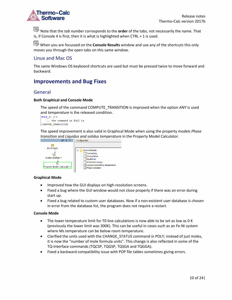
The speed improvement is also valid in Graphical Mode when using the property models Phase transition and Liquidus and solidus temperature in the Property Model Calculator.

Graphical Mode

• Improved how the GUI displays on high-resolution screens. • Fixed a bug where the GUI window would not close properly if there was an error during

start up. • Fixed a bug related to custom user databases. Now if a non-existent user database is chosen

in error from the database list, the program does not require a restart.

Console Mode

• The lower temperature limit for T0 line calculations is now able to be set as low as 0 K (previously the lower limit was 300K). This can be useful in cases such as an Fe-Ni system where Ms temperature can be below room temperature.

• Clarified the units used with the CHANGE_STATUS command in POLY; instead of just moles, it is now the “number of mole formula units”. This change is also reflected in some of the TQ-Interface commands (TQCSP, TQGSP, TQSGA and TQGGA).

• Fixed a backward compatibility issue with POP file tables sometimes giving errors.


11 of 24|

Activity Nodes (e.g. System Definer and Calculators) (Graphical Mode) • A higher contrast for selected and deselected elements in the System Definer Configuration

window is implemented. • Fixed a bug where Binary Calculator or Ternary Calculator predecessors could not be added

to a Plot Renderer. This was applicable when you had more than one Binary or Ternary Calculator.

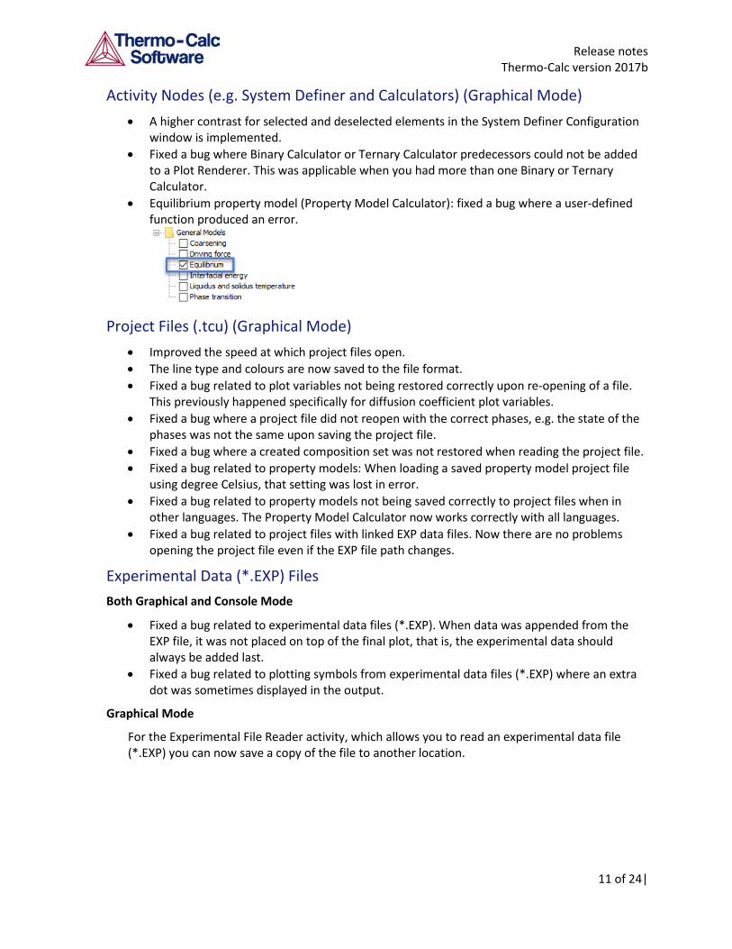
• Equilibrium property model (Property Model Calculator): fixed a bug where a user-defined function produced an error.

Project Files (.tcu) (Graphical Mode) • Improved the speed at which project files open. • The line type and colours are now saved to the file format. • Fixed a bug related to plot variables not being restored correctly upon re-opening of a file.

This previously happened specifically for diffusion coefficient plot variables. • Fixed a bug where a project file did not reopen with the correct phases, e.g. the state of the

phases was not the same upon saving the project file. • Fixed a bug where a created composition set was not restored when reading the project file. • Fixed a bug related to property models: When loading a saved property model project file

using degree Celsius, that setting was lost in error. • Fixed a bug related to property models not being saved correctly to project files when in

other languages. The Property Model Calculator now works correctly with all languages. • Fixed a bug related to project files with linked EXP data files. Now there are no problems

opening the project file even if the EXP file path changes.

Experimental Data (*.EXP) Files Both Graphical and Console Mode

• Fixed a bug related to experimental data files (*.EXP). When data was appended from the EXP file, it was not placed on top of the final plot, that is, the experimental data should always be added last.

• Fixed a bug related to plotting symbols from experimental data files (*.EXP) where an extra dot was sometimes displayed in the output.

Graphical Mode

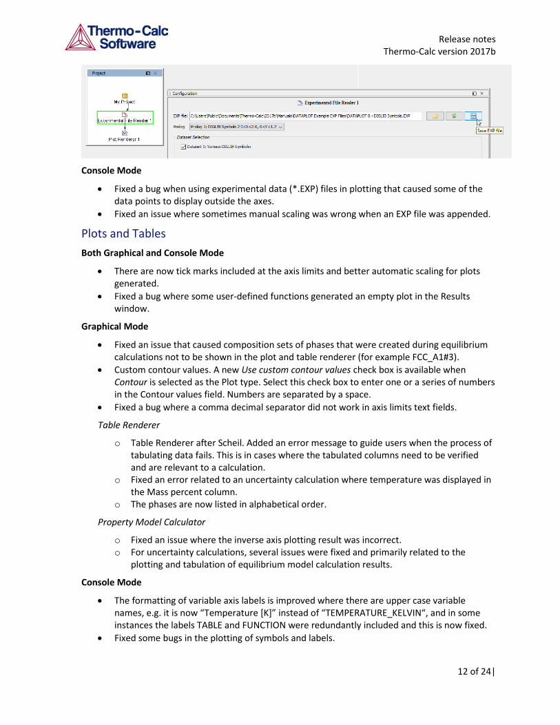
For the Experimental File Reader activity, which allows you to read an experimental data file (*.EXP) you can now save a copy of the file to another location.


12 of 24|

Console Mode

• Fixed a bug when using experimental data (*.EXP) files in plotting that caused some of the data points to display outside the axes.

• Fixed an issue where sometimes manual scaling was wrong when an EXP file was appended.

Plots and Tables Both Graphical and Console Mode

• There are now tick marks included at the axis limits and better automatic scaling for plots generated.

• Fixed a bug where some user-defined functions generated an empty plot in the Results window.

Graphical Mode

• Fixed an issue that caused composition sets of phases that were created during equilibrium calculations not to be shown in the plot and table renderer (for example FCC_A1#3).

• Custom contour values. A new Use custom contour values check box is available when Contour is selected as the Plot type. Select this check box to enter one or a series of numbers in the Contour values field. Numbers are separated by a space.

• Fixed a bug where a comma decimal separator did not work in axis limits text fields.

Table Renderer

o Table Renderer after Scheil. Added an error message to guide users when the process of tabulating data fails. This is in cases where the tabulated columns need to be verified and are relevant to a calculation.

o Fixed an error related to an uncertainty calculation where temperature was displayed in the Mass percent column.

o The phases are now listed in alphabetical order.

Property Model Calculator

o Fixed an issue where the inverse axis plotting result was incorrect. o For uncertainty calculations, several issues were fixed and primarily related to the

plotting and tabulation of equilibrium model calculation results.

Console Mode

• The formatting of variable axis labels is improved where there are upper case variable names, e.g. it is now “Temperature [K]” instead of “TEMPERATURE_KELVIN“, and in some instances the labels TABLE and FUNCTION were redundantly included and this is now fixed.

• Fixed some bugs in the plotting of symbols and labels.


13 of 24|

• Fixed a bug that caused the software to crash if a function was entered incorrectly in the POST module. In this case it was when an extra dot (.) was added after the function name, e.g. h.t.

• Improved the automatic scaling of plots. Previously the automatic range was frequently too large, especially for Scheil-calculations the lower limit was often even negative.

• Improved the automatic pre-settings for the liquidus projection in the Ternary module. • Fixed an issue related to exported tables where lines got cut off after 80 characters.

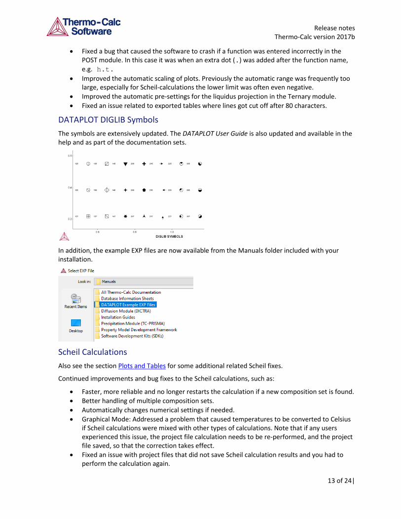
DATAPLOT DIGLIB Symbols The symbols are extensively updated. The DATAPLOT User Guide is also updated and available in the help and as part of the documentation sets.

In addition, the example EXP files are now available from the Manuals folder included with your installation.

Scheil Calculations Also see the section Plots and Tables for some additional related Scheil fixes.

Continued improvements and bug fixes to the Scheil calculations, such as:

• Faster, more reliable and no longer restarts the calculation if a new composition set is found. • Better handling of multiple composition sets. • Automatically changes numerical settings if needed. • Graphical Mode: Addressed a problem that caused temperatures to be converted to Celsius

if Scheil calculations were mixed with other types of calculations. Note that if any users experienced this issue, the project file calculation needs to be re-performed, and the project file saved, so that the correction takes effect.

• Fixed an issue with project files that did not save Scheil calculation results and you had to perform the calculation again.


14 of 24|

Batching Improvements Improvements have been made to how Thermo-Calc performs when batch jobs are run from a custom macro file. For example, when Thermo-Calc is launched to run a single macro after which it is closed (terminated). These improvements are as follows.

• Thermo-Calc shuts down when the job is finished instead of hanging. • Thermo-Calc "pipes" the output from the macro-calculation to the calling program (Before it

was "silent" and this information was not conveyed). See below for an example. • Up to 10 instances of Thermo-Calc can be launched (previously only 5 instances were

allowed).

For Windows users, the new file to start Thermo-Calc application in batch mode is Thermo-Calc.bat instead of the default Thermo-Calc.exe.

There are no changes to the file to be called for Linux and Mac users.

• For Linux: Thermo-Calc.sh • For Mac Thermo-Calc.command

Piping or Redirecting Data

For users who want to pipe or redirect data from Thermo-Calc running a macro in Console Mode.

This information has changed from a previous technical note.

Windows: Thermo-Calc.bat macro.tcm > results.log

Linux: Thermo-Calc.sh -E < macro.tcm > results.log

Mac: Thermo-Calc.command -E < macro.tcm > results.log

Diffusion Module (DICTRA)

New Graphical Mode Features

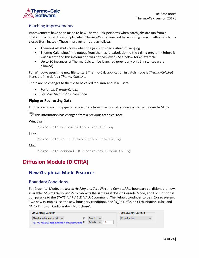
Boundary Conditions For Graphical Mode, the Mixed Activity and Zero Flux and Composition boundary conditions are now available. Mixed Activity and Zero Flux acts the same as it does in Console Mode, and Composition is comparable to the STATE_VARIABLE_VALUE command. The default continues to be a Closed system. Two new examples use the new boundary conditions. See ‘D_06 Diffusion Carburization Tube’ and ‘D_07 Diffusion Carburization Multiphase’.


15 of 24|

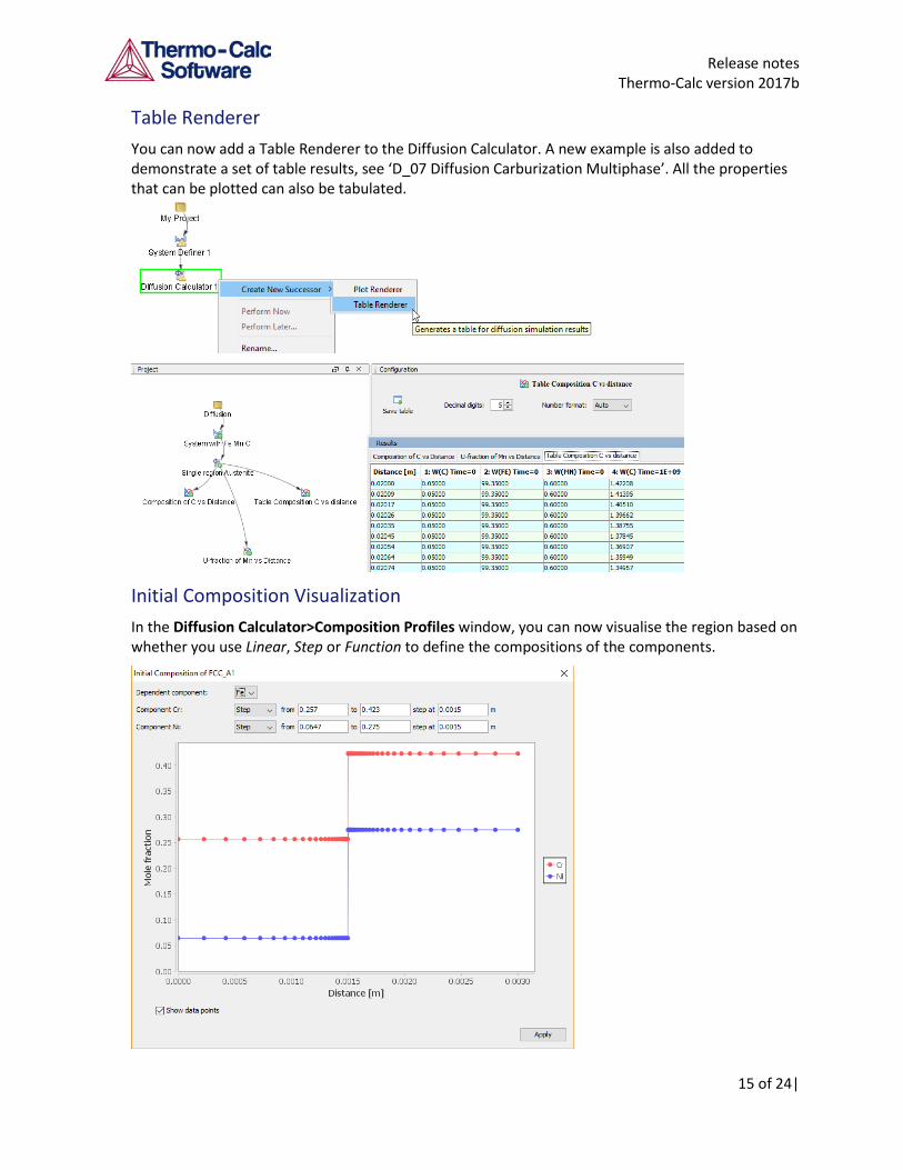
Table Renderer You can now add a Table Renderer to the Diffusion Calculator. A new example is also added to demonstrate a set of table results, see ‘D_07 Diffusion Carburization Multiphase’. All the properties that can be plotted can also be tabulated.

Initial Composition Visualization In the Diffusion Calculator>Composition Profiles window, you can now visualise the region based on whether you use Linear, Step or Function to define the compositions of the components.


16 of 24|

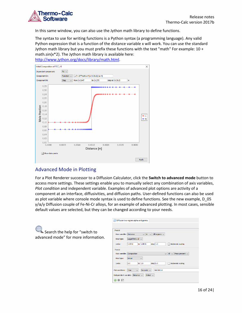
In this same window, you can also use the Jython math library to define functions.

The syntax to use for writing functions is a Python syntax (a programming language). Any valid Python expression that is a function of the distance variable x will work. You can use the standard Jython math library but you must prefix these functions with the text "math" For example: 10 + math.sin(x*2). The Jython math library is available here: http://www.jython.org/docs/library/math.html.

Advanced Mode in Plotting For a Plot Renderer successor to a Diffusion Calculator, click the Switch to advanced mode button to access more settings. These settings enable you to manually select any combination of axis variables, Plot condition and independent variable. Examples of advanced plot options are activity of a component at an interface, diffusivities, and diffusion paths. User-defined functions can also be used as plot variable where console mode syntax is used to define functions. See the new example, D_05 γ/α/γ Diffusion couple of Fe-Ni-Cr alloys, for an example of advanced plotting. In most cases, sensible default values are selected, but they can be changed according to your needs.

Search the help for “switch to advanced mode” for more information.

http://www.jython.org/docs/library/math.html


17 of 24|

New Graphical Mode Examples

D_05 γ/α/γ Diffusion couple of Fe-Ni-Cr alloys This example demonstrates the evolution of a ternary Fe-Cr-Ni diffusion couple. A thin slice of ferrite (α phase) (38%Cr, 0%Ni) is clamped between two thicker slices of austenite (γ phase) (27%Cr, 20%Ni). The assembly is subsequently heat treated at 1373 K. This example demonstrates the use of advanced plotting.

D_06 Diffusion Through a Tube Wall This is a simple example of diffusion through a tube wall. The tube material is an Fe-0.06Mn-0.05C alloy. Two plots comparing distance to the U-fraction of manganese and composition of carbon are generated to visualize the austenite region. A cylindrical geometry is used with mixed zero flux and activity boundary conditions.

On the inside wall a carbon activity of 0.9 is maintained whereas on the outside the carbon activity is very low. This example demonstrates the use of boundary conditions, advanced plotting and tables.

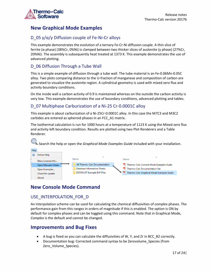
D_07 Multiphase Carburization of a Ni-25 Cr-0.0001C alloy This example is about carburization of a Ni-25Cr-0.0001C alloy. In this case the M7C3 and M3C2 carbides are entered as spheroid phases in an FCC_A1 matrix.

The Isothermal calculation is run for 1000 hours at a temperature of 1123 K using the Mixed zero flux and activity left boundary condition. Results are plotted using two Plot Renderers and a Table Renderer.

Search the help or open the Graphical Mode Examples Guide included with your installation.

New Console Mode Command

USE_INTERPOLATION_FOR_D An interpolation scheme can be used for calculating the chemical diffusivities of complex phases. The performance gain from this ranges in orders of magnitude if this is enabled. The option is ON by default for complex phases and can be toggled using this command. Note that in Graphical Mode, Complex is the default and cannot be changed.


• A bug is fixed so you can calculate the diffusivities of W, Y, and Zr in BCC_B2 correctly. • Documentation bug: Corrected command syntax to be Zerovolume_Species (from

Zero_Volume_Species).


18 of 24|

• Graphical Mode: Corrected the default driving force value in the Tools > Options panel to match that used in the Diffusion Calculator (1e-5).

• Graphical Mode. Fixed a bug that occurred when you switched database packages on the System Definer resulting in incorrect or no species being available for selection on the Diffusion Calculator.

• Graphical Mode: Very small regions are clearly visible in the Configuration Settings window on the Diffusion Calculator.

• Console Mode: Fixed a bug where a simulation would crash the software if it was saving every nth time-step incorrectly.

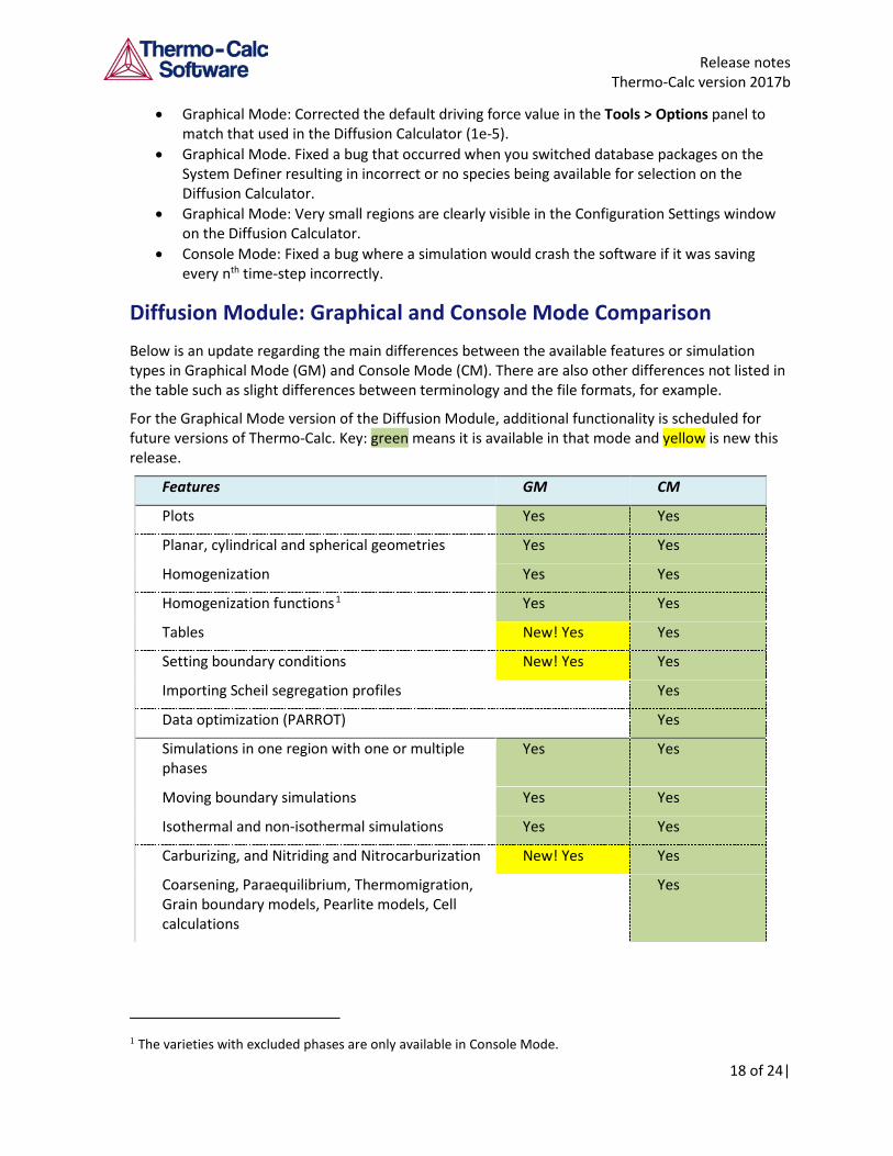
Diffusion Module: Graphical and Console Mode Comparison Below is an update regarding the main differences between the available features or simulation types in Graphical Mode (GM) and Console Mode (CM). There are also other differences not listed in the table such as slight differences between terminology and the file formats, for example.

For the Graphical Mode version of the Diffusion Module, additional functionality is scheduled for future versions of Thermo-Calc. Key: green means it is available in that mode and yellow is new this release.

Features GM CM

Plots Yes Yes

Planar, cylindrical and spherical geometries Yes Yes

Homogenization Yes Yes

Homogenization functions1 Yes Yes

Tables New! Yes Yes

Setting boundary conditions New! Yes Yes

Importing Scheil segregation profiles Yes

Data optimization (PARROT) Yes

Simulations in one region with one or multiple phases

Yes Yes

Moving boundary simulations Yes Yes

Isothermal and non-isothermal simulations Yes Yes

Carburizing, and Nitriding and Nitrocarburization New! Yes Yes

Coarsening, Paraequilibrium, Thermomigration, Grain boundary models, Pearlite models, Cell calculations

Yes

1 The varieties with excluded phases are only available in Console Mode.


19 of 24|

Precipitation Module (TC-PRISMA)

New Calculation Type - Continuous-Cooling Transformation (CCT) You can now plot a CCT diagram with the Precipitation Module. Choose this calculation type on the Precipitation Calculator. A new example (P_07) plots the cooling rate of a Ni-Al-Cr γ-γ’ alloy with superimposition of the cooling rate values. A new video for example P_07 is available on our website and YouTube channel.

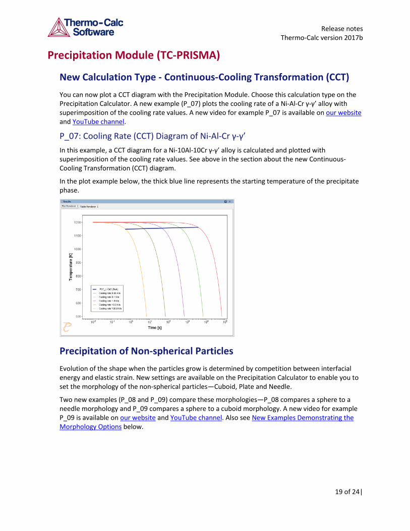
P_07: Cooling Rate (CCT) Diagram of Ni-Al-Cr γ-γ’ In this example, a CCT diagram for a Ni-10Al-10Cr γ-γ’ alloy is calculated and plotted with superimposition of the cooling rate values. See above in the section about the new Continuous-Cooling Transformation (CCT) diagram.

In the plot example below, the thick blue line represents the starting temperature of the precipitate phase.

Precipitation of Non-spherical Particles Evolution of the shape when the particles grow is determined by competition between interfacial energy and elastic strain. New settings are available on the Precipitation Calculator to enable you to set the morphology of the non-spherical particles—Cuboid, Plate and Needle.

Two new examples (P_08 and P_09) compare these morphologies—P_08 compares a sphere to a needle morphology and P_09 compares a sphere to a cuboid morphology. A new video for example P_09 is available on our website and YouTube channel. Also see New Examples Demonstrating the Morphology Options below.


https://www.youtube.com/channel/UCLTh3apGItuaVK69mrwcpJg




20 of 24|

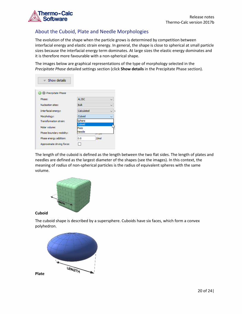
About the Cuboid, Plate and Needle Morphologies The evolution of the shape when the particle grows is determined by competition between interfacial energy and elastic strain energy. In general, the shape is close to spherical at small particle sizes because the interfacial energy term dominates. At large sizes the elastic energy dominates and it is therefore more favourable with a non-spherical shape.

The images below are graphical representations of the type of morphology selected in the Precipitate Phase detailed settings section (click Show details in the Precipitate Phase section).

The length of the cuboid is defined as the length between the two flat sides. The length of plates and needles are defined as the largest diameter of the shapes (see the images). In this context, the meaning of radius of non-spherical particles is the radius of equivalent spheres with the same volume.

Cuboid

The cuboid shape is described by a supersphere. Cuboids have six faces, which form a convex polyhedron.

Plate


21 of 24|

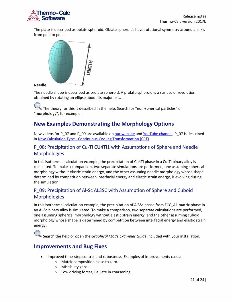
The plate is described as oblate spheroid. Oblate spheroids have rotational symmetry around an axis from pole to pole.

Needle

The needle shape is described as prolate spheroid. A prolate spheroid is a surface of revolution obtained by rotating an ellipse about its major axis.

The theory for this is described in the help. Search for “non-spherical particles” or “morphology”, for example.

New Examples Demonstrating the Morphology Options New videos for P_07 and P_09 are available on our website and YouTube channel. P_07 is described in New Calculation Type - Continuous-Cooling Transformation (CCT).

P_08: Precipitation of Cu-Ti CU4TI1 with Assumptions of Sphere and Needle Morphologies In this isothermal calculation example, the precipitation of Cu4Ti phase in a Cu-Ti binary alloy is calculated. To make a comparison, two separate simulations are performed, one assuming spherical morphology without elastic strain energy, and the other assuming needle morphology whose shape, determined by competition between interfacial energy and elastic strain energy, is evolving during the simulation.

P_09: Precipitation of Al-Sc AL3SC with Assumption of Sphere and Cuboid Morphologies In this isothermal calculation example, the precipitation of Al3Sc phase from FCC_A1 matrix phase in an Al-Sc binary alloy is simulated. To make a comparison, two separate calculations are performed, one assuming spherical morphology without elastic strain energy, and the other assuming cuboid morphology whose shape is determined by competition between interfacial energy and elastic strain energy.

Search the help or open the Graphical Mode Examples Guide included with your installation.


• Improved time-step control and robustness. Examples of improvements cases: o Matrix composition close to zero. o Miscibility gaps. o Low driving forces, i.e. late in coarsening.




22 of 24|

• New time step criterium “Maximum relative solute composition change at each time step” • Documentation: For a Plot Renderer associated to a Precipitation Calculator, improved the

axis variable descriptions (e.g. mean radius, number density, nucleation rate etc.) • Documentation: Improved the descriptions of mobility enhancement prefactor and mobility

enhancement activation energy • Fixed an issue for tables and plots associated to a Precipitation Calculator. Now the units for

nucleation rate and number density are included in plot axes and table headers. • Fixed a bug related to tables and size distribution that crashed the software.

Documentation and Examples

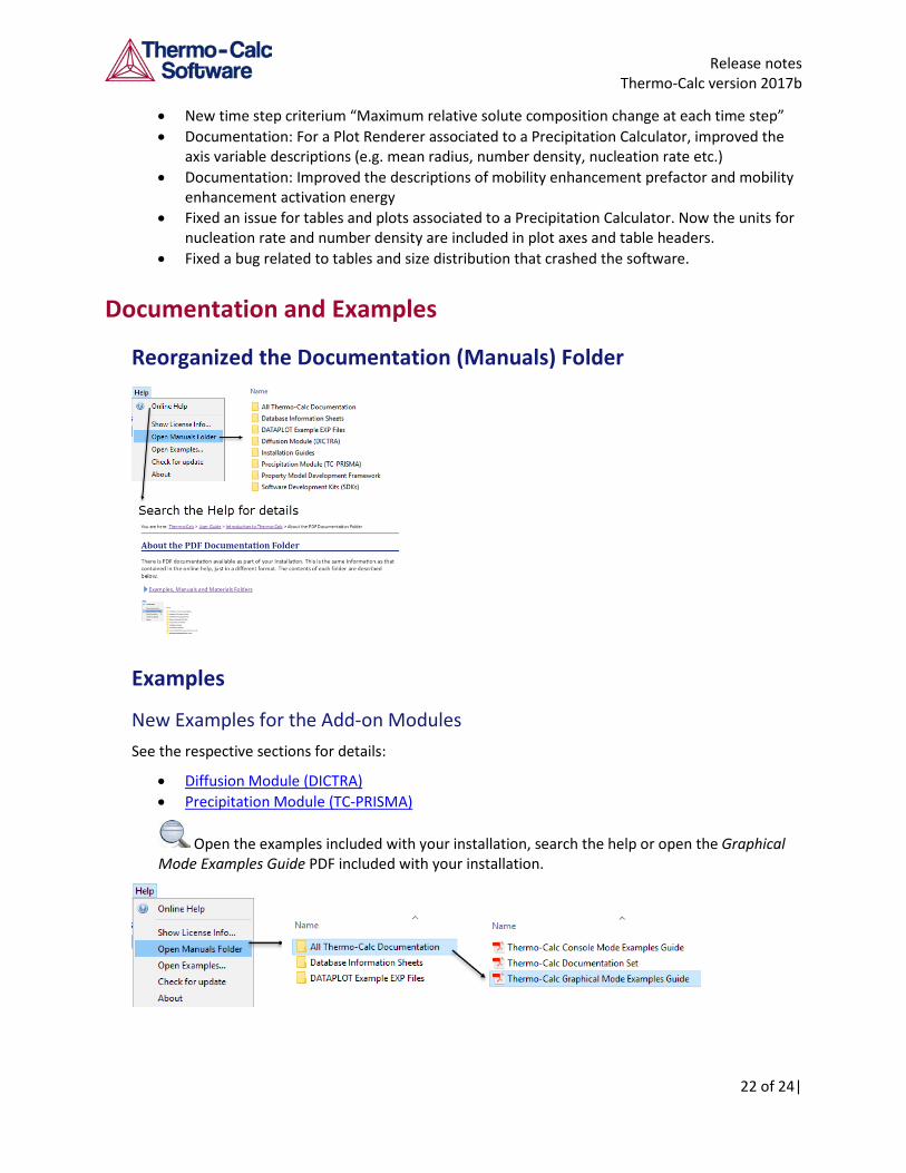
Reorganized the Documentation (Manuals) Folder

Examples

New Examples for the Add-on Modules See the respective sections for details:

• Diffusion Module (DICTRA) • Precipitation Module (TC-PRISMA)

Open the examples included with your installation, search the help or open the Graphical Mode Examples Guide PDF included with your installation.


23 of 24|

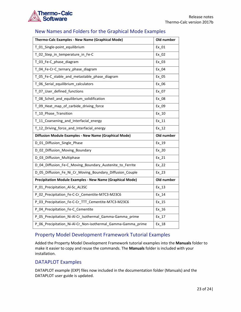
New Names and Folders for the Graphical Mode Examples Thermo-Calc Examples - New Name (Graphical Mode) Old number

T_01_Single-point_equilibrium Ex_01

T_02_Step_in_temperature_in_Fe-C Ex_02

T_03_Fe-C_phase_diagram Ex_03

T_04_Fe-Cr-C_ternary_phase_diagram Ex_04

T_05_Fe-C_stable_and_metastable_phase_diagram Ex_05

T_06_Serial_equilibrium_calculators Ex_06

T_07_User_defined_functions Ex_07

T_08_Scheil_and_equilibrium_solidification Ex_08

T_09_Heat_map_of_carbide_driving_force Ex_09

T_10_Phase_Transition Ex_10

T_11_Coarsening_and_Interfacial_energy Ex_11

T_12_Driving_force_and_Interfacial_energy Ex_12

Diffusion Module Examples - New Name (Graphical Mode) Old number

D_01_Diffusion_Single_Phase Ex_19

D_02_Diffusion_Moving_Boundary Ex_20

D_03_Diffusion_Multiphase Ex_21

D_04_Diffusion_Fe-C_Moving_Boundary_Austenite_to_Ferrite Ex_22

D_05_Diffusion_Fe_Ni_Cr_Moving_Boundary_Diffusion_Couple Ex_23

Precipitation Module Examples - New Name (Graphical Mode) Old number

P_01_Precipitation_Al-Sc_AL3SC Ex_13

P_02_Precipitation_Fe-C-Cr_Cementite-M7C3-M23C6 Ex_14

P_03_Precipitation_Fe-C-Cr_TTT_Cementite-M7C3-M23C6 Ex_15

P_04_Precipitation_Fe-C_Cementite Ex_16

P_05_Precipitation_Ni-Al-Cr_Isothermal_Gamma-Gamma_prime Ex_17

P_06_Precipitation_Ni-Al-Cr_Non-isothermal_Gamma-Gamma_prime Ex_18

Property Model Development Framework Tutorial Examples Added the Property Model Development Framework tutorial examples into the Manuals folder to make it easier to copy and reuse the commands. The Manuals folder is included with your installation.

DATAPLOT Examples DATAPLOT example (EXP) files now included in the documentation folder (Manuals) and the DATAPLOT user guide is updated.


24 of 24|

TQ-Interface Examples For Linux OS, fixed a bug where the TQ-Interface examples in FORTRAN did not run.

For a list of TQ-Interface examples and the installation location, search the help for TQ Examples or TQ-Interface Examples.

New and Updated Training Videos All videos are available on our website and YouTube channel.

• T_08_Scheil_and_equilibrium_solidification • T_09_Heat_Map_of_Carbide_Driving_Force • T_11 is updated to demonstrate the 3D plot. • T_12_Driving_Force_and_Interfacial_Energy • D_07_Diffusion_Carburization_Multiphase • P_07_Precipitation_Ni-Al-Cr_CCT_Gamma-Gamma_prime • P_09_Precipitation_Al-Sc_AL3SC_Sphere_Cuboid • 2017b Release Overview

Installation Disk Space Requirement Due to precompiled databases added to the Thermo-Calc installation, 2 GB of disk space is recommended for the 2017b installation.

Platform Roadmap This is the last release where Windows 32-Bit will be supported.

For information about platforms being phased out visit http://www.thermocalc.com/products-services/software/system-requirements/platformroadmap/.



http://www.thermocalc.com/products-services/software/system-requirements/platformroadmap/

http://www.thermocalc.com/products-services/software/system-requirements/platformroadmap/

Documents

Release Notes: Thermo-Calc Software Package Version 2017b · Release Notes: Thermo-Calc Software Package . Version 2017b . Release notes Thermo-Calc version 2017b . 2 of 24| Contents