Thermalconvectioninliquidbridgeswithcurvedfreesurfaces ...homepages.ulb.ac.be/~dmelniko/Papers/Journal_of_Crystal...Benchmarkofnumericalsolutions ValentinaShevtsova MRC, CP-165/62,

ARTICLE IN PRESS

0022-0248/$ - se

doi:10.1016/j.jcr

�Tel.: +32 2

E-mail addre

URL: http:/

Journal of Crystal Growth 280 (2005) 632–651

www.elsevier.com/locate/jcrysgro

Thermal convection in liquid bridges with curved free surfaces:Benchmark of numerical solutions

Valentina Shevtsova�

MRC, CP-165/62, Universite Libre de Bruxelles, 50, av. F.D. Roosevelt, B-1050 Brussels, Belgium

Received 28 February 2005; accepted 31 March 2005

Available online 23 May 2005

Communicated By T. Hibiya

Abstract

Numerical solutions of thermocapillary and buoyant convection in liquid bridges with curved free interfaces are

benchmarked. The results were presented in the Second International Marangoni Association, IMA-2 Congress,

Brussels, 2004. Only small Prandtl number fluids (Pr � 10�2) are considered. The study consists of two parts:

(1) investigation of axisymmetric steady states in curved liquid bridges in a wide range of contact angles and different

gravity conditions; (2) calculation of critical Reynolds numbers for the first stationary bifurcation with straight and

concave interfaces. The numerical simulations were performed for two aspect ratios G ¼ 1 and 1.2.

Nine research groups participated in this effort and are thus considered co-authors of the present manuscript. Because

all the groups employed body-fitted curvilinear coordinates for solving the Navier–Stokes and energy equations a brief

description of this method is presented.

r 2005 Elsevier B.V. All rights reserved.

PACS: 47.11.þj; 47.20.Dr; 81.10.Fq; 83.50.�v

Keywords: A1. Interfaces; A1. Computer simulation; A1. Convection; A2. Floating zone technique; A2. Microgravity conditions

1. Introduction

Surface tension can vary locally due to tem-perature or concentration gradients along liquid–gas interfaces. Thermocapillary convection drivenby these tangential stresses is gravity independent.

e front matter r 2005 Elsevier B.V. All rights reserve

ysgro.2005.03.092

650 30 24; fax: +32 2 650 31 26.

ss: [email protected].

/www.ulb.ac.be/polytech/mrc.

At ground conditions the flow is modified by therelatively strong influence of buoyancy forces. Thethermoconvective flow is of particular importancein the floating zone crystal growth technique. Thehalf-zone model (liquid bridge) is used as anapproximation of the side-heated liquid zoneassuming that the flow in this latter configurationis reflection-symmetric with respect to the hor-izontal mid-plane. To simplify the model it is quitereasonable in a first approach to neglect the

d.

www.elsevier.com/locate/jcrysgro

ARTICLE IN PRESS

V. Shevtsova / Journal of Crystal Growth 280 (2005) 632–651 633

complexities of phase change and to focus on bulkconvection.Extensive knowledge concerning transition from

steady to oscillatory states in liquid bridges hasbeen gained from numerous experiments andnumerical simulations, see overviews by Kuhl-mann [1] and Schatz and Neitzel [2]. Ground-based experiments deal with tiny liquid bridges toreduce buoyant convection. In order to eliminatebuoyancy effects experiments have been performedin low-gravity environments and have demon-strated that thermocapillary convection alone caninduce instabilities, e.g. Refs. [3,4]. Recent studiesinvestigate the role of secondary effects on thedevelopment of non-steady flow patterns in liquidbridges: free-surface deformation, heat exchangewith gas environment, and extremely short orlong bridges, etc. Among these free-surface defor-mations have been investigated by several re-searchers.With respect to the stability of convection in

deformable liquid bridges, theoretical develop-ments are not as advanced as experimental results.The first calculations on steady thermocapillaryconvection in a floating zone with a deformablefree surface were done by Kozhoukharova andSlavchev [5] for small deformations. The thermo-capillary flow near the cold corner was consideredby Shevtsova et al. [6] in liquid bridges with Pr ¼

1:0 and a wide range of contact angles. A study ofthe viscous flow in a wedge between a rigidplane and a liquid surface with a constantshear stress was given by Kuhlmann et al. [7].Shevtsova and Legros [8] investigated transitionfrom steady axisymmetric flows to oscillatoryregimes in silicone oil ðPr ¼ 105Þ liquid bridgesincluding the effects of free surfaces with largestatic deformations. They reported buoyant-thermocapillary instabilities with m ¼ 0 forrelatively low Marangoni numbers and ~ga0;he steady state was unstable to axially runningwaves. Using linear stability analysis (LSA) Chenand Hu [9] determined the onset of oscillatoryinstability for Pr ¼ 1; 10 and 50 and zero gravity(~g ¼ 0).Recently, significant progress in the study of

transition from 2D steady states to steady 3Dconvection in liquid metals has been achieved.

Marangoni convection with statically deformedfree surfaces with Pr ¼ 0:001; 0:01; 0:02 was com-puted by Chen et al. [10], Lappa et al. [11] andNienhuser et al. [12,13].Transition to oscillatory 3D states in high

Prandtl number liquids have also been consideredby Sumner et al. [14], Tang et al. [15], Sim andZebib [16], and Ermakov and Ermakova [17]. Theclosely related case of annuli with free interfaceswas considered by Kamotani et al. [18] and Simand Zebib [19].The first attempt to capture dynamic free-

surface deformations in liquid bridges was re-ported by Shevtsova et al. [20]. For small capillarynumbers Ca51 they showed that the amplitude ofinterface oscillations is very small and is onlyabout 1% of the static shape with Pr ¼ 105. Theamplitude of free-surface oscillation varied alongthe axial coordinate with a maximum near thehot corner.Kuhlmann et al. [21] performed a detailed

study of dynamic free-surface deformations inliquid bridges with Pr ¼ 0:02 and 4.38 usingan asymptotic expansion in the limit Ca ! 0 incombination with LSA. As in the case ofrectangular cavities considered by Mundraneand Zebib [22] they concluded that surfacedeformations are caused by lower-order flowfields. Thus, in both geometries dynamic deforma-tions did not play a dominant role in the onset ofoscillations.The numerical results for thermocapillary flows

in deformed liquid bridges should be consideredwith care because of discrepancies in the publishedresults. For this reason it was decided in the frameof the IMA-2 Congress, Brussels, Belgium 2004(http://www.ulb.ac.be/polytech/mrc/ima2.html) tobenchmark 2D and 3D flows in liquid bridges withstatically deformed interfaces. Accordingly, all theparticipants in this benchmark are co-authors ofthe present manuscript. Results of the nineparticipating groups employing different numer-ical codes are given in the manuscript according tothe acronyms listed in Table 1. All the nine groupsutilize the body-fitted method for transforming thecoordinate system although it was not requested.This method has also been used in the majority ofpreviously published results on this subject.

http://www.ulb.ac.be/polytech/mrc/ima2.html

ARTICLE IN PRESS

Table 1

Benchmark participants; IMA-2 14–17 July 2004, Brussels

Acronyms Names, contact e-mail City, Country Code info

1 CLR G. Chen, C.W. Lan, B. Roux University of Marseille, France BF

[email protected] LSA

2. DKL S. Domesi, H.C. Kuhlmann, J. Leypoldt Tech.University of Vienna, Austria WD

[email protected]

3. EE M.K. Ermakov, M.S. Ermakova Inst. for Problems in Mech., Moscow, Russia BF

[email protected] LSA

4. FK K. Fukui, H. Kawamura Tokyo University of Science, Japan BF

[email protected]

5. SH S. Shiratori, T. Hibiya Tokyo Metropolitan University, Japan WD

[email protected]/[email protected] LSA

6. MSL D. Melnikov, V. Shevtsova, J.C. Legros Brussels University, Belgium BF

[email protected]

7. LI K. Li, N. Imaishi Kyushu University, Japan WD

[email protected]

8. SL V. Shevtsova, J.C. Legros Brussels University, Belgium BF

[email protected]

9. SZ B.-C. Sim, A. Zebib Rutgers University, NJ, USA BF

[email protected]

V. Shevtsova / Journal of Crystal Growth 280 (2005) 632–651634

The last column in Table 1 indicates that either thebody-fitted (BF) method was applied or that theparticular group only considered the problemwithout deformation (WD).

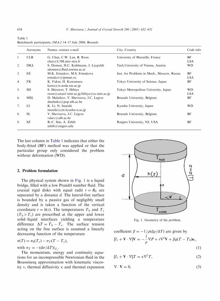
Fig. 1. Geometry of the problem.

2. Problem formulation

The physical system shown in Fig. 1 is a liquidbridge, filled with a low Prandtl number fluid. Thecoaxial rigid disks with equal radii r ¼ R0 areseparated by a distance d. The lateral-free surfaceis bounded by a passive gas of negligibly smalldensity and is taken a function of the verticalcoordinate r ¼ hðzÞ. The temperatures Th and T c

(Th4T c) are prescribed at the upper and lowersolid–liquid interfaces yielding a temperaturedifference DT ¼ Th � Tc. The surface tensionacting on the free surface is assumed a linearlydecreasing function of the temperature

sðTÞ ¼ s0ðTcÞ � sT ðT � TcÞ,

with sT ¼ �ðds=dTÞjT c.

The momentum, energy and continuity equa-tions for an incompressible Newtonian fluid in theBoussinesq approximation with kinematic viscos-ity n, thermal diffusivity k and thermal expansion

coefficient b ¼ �1=rðdr=dTÞ are given by

½qt þ V r�V ¼ �1

rrP þ nr2Vþ bgðT � T0Þez,

(1)

½qt þ V r�T ¼ kr2T , (2)

r V ¼ 0, (3)

ARTICLE IN PRESS


where the velocity, pressure and temperature aredenoted as V, T and P.The stress balance between the viscous fluid

and the inviscid gas on the non-flat free surfacer ¼ hðzÞ is given by

½P � P0 þ sðr.nÞ�ni ¼ Siknk þ si rr, (4)

where Sik ¼ mðqVi=qxk þ qVk=qxiÞ is the viscousstress tensor, P and P0, are the liquid and ambientgas pressures, and sðr nÞ is the Laplace pressure.The tangential projections of Eq. (4) define the

driving thermocapillary force

sz.S.nþ qs=qsz ¼ 0, (5)

sj S nþ qs=qsj ¼ 0, (6)

where sz and su are the unit tangential vectors tothe free surface in r–z and r–j planes, respectively,and n is the unit normal vector directed out ofliquid into the ambient gas. The location of theinterface r ¼ hðz; tÞ is determined by the normalprojection

DP0nþ rgðd � zÞn ¼ n.S.n� sr.n. (7)

The mean curvature is

r n ¼1

R1þ

1

R2

� �,

where R1 and R2 are the principal radii of interfacecurvature.The condition that the fluid at the free surface

r ¼ hðz; tÞ flows along the boundary and neverleaves the interface results in kinematic boundarycondition

n.V ¼1ffiffiffiffiffiffiffiffiffiffiffiffiffiffiffiffiffiffiffiffiffiffiffiffiffiffi

1þ ðdh=dzÞ2q qh

qt: ð8Þ

The free surface is assumed thermally insulated

n.rT ¼ 0. (9)

Table 2

Physical scales

Variable t z r; h V r;Vj;Vz

Scale d2=n d R0 n=d

The boundary conditions on the rigid wallscomplete the problem specification. No slip con-ditions are imposed for the velocity

V ¼ 0 at z ¼ 0; d ð10Þ

and the temperature at the rigid walls is constant

Tz¼0 ¼ Tc at Tz¼d ¼ Th. (11)

3. Mathematical aspects

The motion is referred to a cylindrical coordi-nate system with the velocity V ¼ ðVr;Vj;VzÞ.For 2D solutions the Stokes stream function c is

Vr ¼ �1

r

qcdz

; V z ¼1

r

qcdr

.

The physical quantities are non-dimensionalizedwith respect to the scales given in Table 2.Note that two characteristic length scales d and

R0 are used for the vertical and radial coordinates,respectively. Thus, r ¼ ½Gqr; ðG=rÞqj; qz�. Thetemperature deviation from the linear profile ~T ¼

Yþ z was also employed by some participants.With these characteristic scales Eqs. (1)–(11)

include few typical dimensionless parameters: thePrandtl, Reynolds, Grashof and dynamic Bondnumbers,

G ¼d

R0; Pr ¼

nk; Re ¼

sTDTd

r0n2,

Gr ¼gbDTd3

n2; Bodyn ¼

Gr

Re¼

grbd2

sT

. ð12Þ

The dynamic Bond number measures the relativestrength of the buoyancy force compared to thethermocapillary force. Instead of Re and Gr, theMarangoni number Ma ¼ Re Pr and Rayleighnumber Ra ¼ Gr Pr can be used.

c P T Vol

nd rðn=dÞ2 ~T ¼ ðT � T cÞ=DT pR20d

ARTICLE IN PRESS


The free-surface shape is controlled by thecharacteristic capillary ðs0=dÞ, hydrostatic ðrgdÞ

and hydrodynamic ðsTDT=dÞ pressures, andthe viscous force per unit area Pscale ¼

rV 2scale ¼ rðn=dÞ2. Thus, the dimensionless version

of the interface boundary conditions Eqs. (5)–(7)includes combination of these quantities. Themagnitude of the static deformation of the inter-face depends on the static Bond number which isthe ratio of the hydrostatic to the capillarypressure

Bo ¼ðrgdÞ

ðs0=dÞ¼

rgd2

s0. (13)

The Capillary number provides a measure of themagnitude of dynamic free-surface deformations.One may define the Capillary number in twodifferent manners: Ca as the ratio of the hydro-dynamic pressure to the typical capillary pressureor C as the ratio of the viscous force per unit areato the typical capillary pressure. These Capillarynumbers are coupled through the Reynoldsnumber

Ca ¼ðsTDT=dÞ

ðs0=dÞ¼

sTDT

s0; C ¼

ðrn2=d2Þ

ðs0=dÞ¼

rn2

s0d,

Ca ¼ C Re. ð14Þ

In most liquid bridge experiments C51 andCao1. The small value of Capillary number, Ca,corresponds to the case of small surface tensionvariation as compared to the mean surface tensionand thus the dynamic free-surface deformationscan be neglected. It is usually assumed that Ca andC have the same order of magnitude, i.e.OðCaÞ � OðCÞ, see Ref. [21].The moving boundary problem Eqs. (1)–(11)

can be solved by perturbation methods in theasymptotic limit of small Capillary numberCa;C ! 0. Taking into account that quantitieswith tilde denote a dimensionless value we have

s ¼ s0 � gðT � T0Þ ¼ s0½1� Ca ~T � and

~DP ¼ ðDP0 þ rgdÞ=Pch,

Eq. (7) becomes

D ~P �Bost

Cz ¼ n. ~S.n�

1

Cð1� Ca ~TÞ G ~r n. (15)

The Laplace pressure, the last term in Eq. (15), inthe limit C ! 0 can only be balanced by thehydrostatic pressure jump between the fluid in theliquid bridge and the ambient gas. This pressurejump is asymptotically large, 1=C or 1=Ca.Thus, the following expansions are used to find theleading order contributions to the flow andtemperature fields (henceforth, we drop the tildeand all variables are dimensionless):

f ðr; zÞ ¼ f 0ðr; zÞ þ C f 1ðr; zÞ þ OðC2Þ,

~P ¼ C�1Pst þ P0 þ C P1 þ OðC2Þ,

~h ¼ h0ðzÞ þ Ch1ðr; zÞ þ OðC2Þ, ð16Þ

here f ðr; z; tÞ reads for the components of velocityvector—V, temperature—T and volume—Vol.The Capillary number C ! 0 is used as the smallparameter for the asymptotic expansion.The perturbation method splits the solution in a

few steps: first the shape of interface is accuratelydetermined in a static configuration; then thecomplete moving boundary problem transformsinto a convection problem with the previouslycalculated free-surface location. At the next pointdynamic surface deformations are determinedfrom the flow field computed in the previous step.This approach was used by Shevtsova et al. [20],Kuhlmann et al. [21] in liquid bridge problems. Inthe present benchmark the solution is limited toOðC0Þ and dynamic surface deformations were notcalculated. Comparable small effects should betaken into account at OðC1Þ and higher orders, e.g.highest order terms in Boussinesq expansion, thechange of the liquid volume due to thermalexpansion, etc. Calculations at OðC1Þ are straight-forward and were done for a rectangular cavity inRef. [22].The solution at lowest order, e.g. OðC�1Þ

determines the hydrostatic free-surface shape.The position of the free surface, r ¼ hðzÞ is thusindependent of the flow. Taking into account thatthe projections of the unit vectors are

~n ¼1ffiffiffiffiffiffiffiffiffiffiffiffiffiffiffiffiffiffiffiffiffiffiffiffiffi

ð1þ G�2h02Þ

q ½1; 0;�h0=G�,

~tz ¼1ffiffiffiffiffiffiffiffiffiffiffiffiffiffiffiffiffiffiffiffiffiffiffiffiffi

ð1þ G�2h02Þ

q ½h0=G; 0; 1�; ~tj ¼ ½0; 1; 0�,

ARTICLE IN PRESS


where the superscript 0 denotes the derivative, e.g.h0

¼ dh=dz. The dimensionless mean curvaturebecomes

~r n ¼1

R1þ

1

R2

¼1

ð1þ G�2h02Þ1=2

h00

G2ð1þ G�2h02Þ�1

h

� �.

Eq. (15) transforms into the Young–Laplaceequation for the static meniscus shape

DPst � Bostz ¼1

N

1

h0�

h000

G2N2

� �; where

N ¼

ffiffiffiffiffiffiffiffiffiffiffiffiffiffiffiffiffiffiffiffiffiffiffiffiffið1þ G�2h02

0 Þ

q. ð17Þ

The boundary conditions associate with thesecond-order ordinary differential equationEq. (17) are

(1)
constant fluid volume (scaled by V cyl ¼ pR2d)Vol0 ¼
R 10 h20ðzÞdz,

(2)
fixed contact points h0ð0Þ ¼ h0ð1Þ ¼ 1, (3) fixed contact angles: G�1 hzð0Þ ¼ � cot ac or
G�1 hzð1Þ ¼ cot ah.

Here the angles ac and ah are measured from therigid disks to the free surface. Thus, threeboundary conditions can be applied to solve theordinary differential equation of the second order.Any two of these conditions may be used for thesolution of Eq. (17) and a third determines DPst.At OðCa0Þ the governing equations are identical tothe initial Eqs. (1)–(3)

qV0

qtþ V0.rV0 ¼ �rP0 þr2V0 þ Gr T0ez, ð18Þ

qT0

qtþ V0 rT0 ¼

1

Pr r2T0, ð19Þ

r V0 ¼ 0. ð20Þ

The boundary conditions are to be applied at thefixed boundary r ¼ h0ðzÞ.The tangential balance equations (5)–(6) become

(Z ¼ nr)

1

Nð1� G�2h02

0 Þ GqVz0

qrþ

qV r0

qz

� ��

þ2h0

0

GGqV r0

qr�

qV z0

qz

� ��

¼ �Re h00

qT0

qrþ

qT0

qz

� �, ð21Þ

1

N

qVj0

qr�

Vj0

rþ1

r

qV r0

qj�

h00

GG�1 qVj0

qz

��

þ1

r

qV z0

qj

��¼ �Re

1

r

qT0

qj. ð22Þ

The free surface remains motionless and thekinematic condition leads to

Vn ¼1ffiffiffiffiffiffiffiffiffiffiffiffiffiffiffiffiffiffiffiffiffiffiffiffiffi

ð1þ G�2h020 Þ

q ðVr0 � h00V z0Þ

¼1ffiffiffiffiffiffiffiffiffiffiffiffiffiffiffiffiffiffiffiffiffiffiffiffiffi

ð1þ G�2h020 Þ

q qh

qt¼ 0 thus Vr0 ¼ h0

0Vz0.

The free surface is assumed thermally insulated

qnYðr ¼ h0;j; z; tÞ ¼ 0.

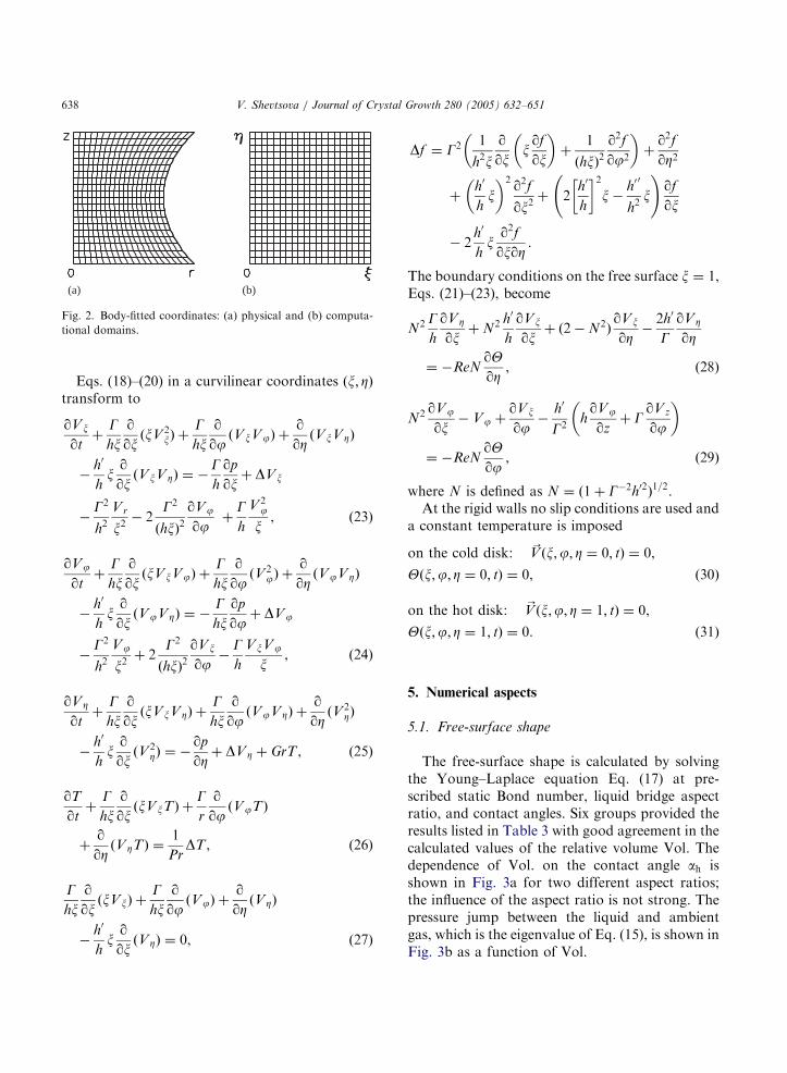
4. Body-fitted coordinate transformation

Here and below h0¼ dh=dx and h00

¼ d2h=d2x.The static free-surface shape does not depend onthe azimuthal coordinate. In the new variables theradial coordinate x varies from x ¼ 0 at the axis, tox ¼ 1 at the free surface and the axial coordinatearies from Z ¼ 0 at the cold disk up to Z ¼ 1 at thehot disk. To simplify notation the subscript ‘‘0’’,denoting OðC0Þ, is dropped.Detailed description is given here because of

discrepancies in the literature. The original physi-cal domain in the ðr; zÞ plane (see Fig. 2) istransformed into a rectangular computationaldomain in the ðx; ZÞ plane by the transformations

x ¼ r=hðzÞ; Z ¼ z !qqr

¼1

h

qqx

,

qqz

¼qqZ

� xh0

h

qqx

,

Vr ¼ Vx; Vz ¼ V Z,

velocities are not transformed.

ARTICLE IN PRESS

(a) (b)

Fig. 2. Body-fitted coordinates: (a) physical and (b) computa-

tional domains.


Eqs. (18)–(20) in a curvilinear coordinates ðx; ZÞtransform to

qV x

qtþ

Ghx

qqx

ðxV 2xÞ þ

Ghx

qqj

ðV xVjÞ þqqZ

ðV xV ZÞ

�h0

hxqqx

ðV xV ZÞ ¼ �Gh

qp

qxþ DVx

�G2

h2V r

x2� 2

G2

ðhxÞ2qVj

qjþ

Gh

V 2j

x, ð23Þ

qVj

qtþ

Ghx

qqx

ðxV xVjÞ þGhx

qqj

ðV2jÞ þ

qqZ

ðVjV ZÞ

�h0

hxqqx

ðVjVZÞ ¼ �Ghx

qp

qjþ DVj

�G2

h2Vj

x2þ 2

G2

ðhxÞ2qV x

qj�

Gh

V xVj

x, ð24Þ

qV Z

qtþ

Ghx

qqx

ðxV xV ZÞ þGhx

qqj

ðVjV ZÞ þqqZ

ðV 2ZÞ

�h0

hxqqx

ðV 2ZÞ ¼ �

qp

qZþ DV Z þ GrT , ð25Þ

qT

qtþ

Ghx

qqx

ðxV xTÞ þGr

qqj

ðVjTÞ

þqqZ

ðV ZTÞ ¼1

PrDT , ð26Þ

Ghx

qqx

ðxVxÞ þGhx

qqj

ðVjÞ þqqZ

ðVZÞ

�h0

hxqqx

ðV ZÞ ¼ 0, ð27Þ

Df ¼ G2 1

h2x

qqx

xqf

qx

� �þ

1

ðhxÞ2q2fqj2

� �þ

q2fqZ2

þh0

hx

� �2 q2f

qx2þ 2

h0

h

� �2x�

h00

h2x

!qf

qx

� 2h0

hxq2fqxqZ

.

The boundary conditions on the free surface x ¼ 1,Eqs. (21)–(23), become

N2 Gh

qV Z

qxþ N2 h0

h

qV x

qxþ ð2� N2Þ

qVx

qZ�2h0

GqV Z

qZ

¼ �ReNqYqZ

, ð28Þ

N2 qVj

qx� Vj þ

qVx

qj�

h0

G2hqVj

qzþ G

qV z

qj

� �

¼ �ReNqYqj

, ð29Þ

where N is defined as N ¼ ð1þ G�2h02Þ1=2.

At the rigid walls no slip conditions are used anda constant temperature is imposed

on the cold disk: ~V ðx;j; Z ¼ 0; tÞ ¼ 0,

Yðx;j; Z ¼ 0; tÞ ¼ 0, ð30Þ

on the hot disk: ~V ðx;j; Z ¼ 1; tÞ ¼ 0,

Yðx;j; Z ¼ 1; tÞ ¼ 0. ð31Þ

5. Numerical aspects

5.1. Free-surface shape

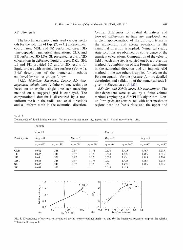
The free-surface shape is calculated by solvingthe Young–Laplace equation Eq. (17) at pre-scribed static Bond number, liquid bridge aspectratio, and contact angles. Six groups provided theresults listed in Table 3 with good agreement in thecalculated values of the relative volume Vol. Thedependence of Vol. on the contact angle ah isshown in Fig. 3a for two different aspect ratios;the influence of the aspect ratio is not strong. Thepressure jump between the liquid and ambientgas, which is the eigenvalue of Eq. (15), is shown inFig. 3b as a function of Vol.

ARTICLE IN PRESS


5.2. Flow field

The benchmark participants used various meth-ods for the solution of Eqs. (23)–(31) in curvilinearcoordinates. MSL and SZ performed direct 3Dtime-dependent numerical simulations. CLR andEE performed 3D LSA. SL presented results of 2Dcalculations in deformed liquid bridges. DKL, SH,LI and FK provided 3D and/or 2D results forliquid bridges with straight free surfaces (Vol ¼ 1).Brief descriptions of the numerical methodsemployed by various groups follow.

MSL: Melnikov, Shevtsova, Legros; 3D time-

dependent calculations: A finite volume techniquebased on an explicit single time step marchingmethod on a staggered grid is employed. Thecomputational domain is discretized by a non-uniform mesh in the radial and axial directionsand a uniform mesh in the azimuthal direction.

Table 3

Dependence of liquid bridge volume—Vol on the contact angle—ah,

Volume

G ¼ 1:0

Participants Bost ¼ 0 Bost ¼ 5

ah ¼ 40� ah ¼ 140� ah ¼ 60� ah ¼ 9

CLR 0.685 1.348 0.97 1.173

EE 0.685 1.348 0.970 1.173

FK 0.69 1.350 0.97 1.17

MSL 0.685 1.348 0.97 1.173

SL 0.685 1.348 0.97 1.173

SZ 0.681 1.350 — —

(a) (b)

Fig. 3. Dependence of (a) relative volume on the hot corner contact

volume Vol; Bost ¼ 0.

Central differences for spatial derivatives andforward differences in time are employed. Animplicit approximation of the diffusion terms inthe momentum and energy equations in theazimuthal direction is applied. Numerical steadystate solutions are obtained by convergence of thetransient calculations. Computation of the velocityfield at each time step is carried out by a projectionmethod. A combination of fast Fourier transformsin the azimuthal direction and an implicit ADImethod in the two others is applied for solving thePoisson equation for the pressure. A more detaileddescription and validation of the numerical code isgiven in Shevtsova et al. [23].

SZ: Sim and Zebib; direct 3D calculations: Thetime-dependent were solved by a finite volumemethod employing a SIMPLER algorithm. Non-uniform grids are constructed with finer meshes inregions near the free surface and the upper and

aspect ratio—G and gravity level—Bost

G ¼ 1:2

Bost ¼ 0 Bost ¼ 5

0� ah ¼ 40� ah ¼ 140� ah ¼ 60� ah ¼ 90�

0.620 1.425 0.965 1.215

0.620 1.425 0.965 1.215

0.620 1.43 0.965 1.210

0.62 1.425 0.965 1.215

0.62 1.425 0.965 1.215

0.616 1.428 — —

angle—ah and (b) the interfacial pressure jump on the relative

ARTICLE IN PRESS


lower walls where boundary layers develop. Amesh of 51ðxÞ � 61ðZÞ with regularization is used in2D simulations. In the 3D model a mesh of 41ðxÞ �41ðZÞ � 40ðjÞ is used. For the transition fromaxisymmetric (2D) to steady non-axisymmetric(3D) flow Re is varied in increments of 10 toestimate the critical Reynolds number, Recr. Thesesteps in Re, DRe ¼ 10, are less than 1% of thereported Recr at the first stationary bifurcation.Validation of the code is in Sim and Zebib [16].

EE: Ermakov and Ermakova; 3D LSA: The basicaxisymmetric flow is computed on a staggered gridby a finite volume technique. Regularization wasnot employed to resolve the thin structure near thetop and bottom corners. The 2D discretizedequations are solved directly by iterative New-ton–Raphson procedure with optimal choice ofthe relaxation parameter. Calculations were per-formed on non-uniform 161� 161 grids for thestraight cylinder geometry.The 3D problem was treated as a LSA. Normal

mode perturbations of the form expðlt þ

imjÞð~u; p; tÞTðr; zÞ; m ¼ 0; 1; 2; . . . were considered.The azimuthal wave number m ¼ 0 corresponds to2D axisymmetric perturbations, m ¼ 1 corre-sponds to 3D perturbations with non-zero velocityat the axes line, and m41 corresponds to 3Dperturbation with zero velocity at r ¼ 0. Perturba-tions in the radial and axial directions areapproximated on the same staggered grid as thebasic flow. The governing LSA equations andboundary conditions can be found in Wanschuraet al. [24] and Nienhuser et al. [12]. The LSA studyis reduced to the generalized eigenvalue problemAx ¼ lBx, x 2 Cn (B is a diagonal singular matrix)and was solved by inverse iterations. Inversions ofmatrices are performed by stabilized bi-conjugategradient method with ILU pre-conditioning. Sav-ings in computer memory and time are due to acompact storage scheme and matrix operations forsparse matrices. Typical calculation time is up to10min on a 3.2GHz PC for the steady 2D problemand up to 30min for an LSA calculations (oneeigenvalue/eigenvector set). 2GB RAM was re-quired.

CLR: Chen, Lan, Roux; 3D LSA: Formulationof the full problem was in primitive variables. Thefinite-difference method was used on body-fitted

coordinates. The discretized equations are solveddirectly by iterative Newton–Raphson procedure.The global iteration was used to determine thedynamic free-surface deformation h1ðr; zÞ.LSA was used for the 3D problem. The method

is similar to that used by EE and described above.Special procedure was adopted for locatingbifurcation points of the basic state. The equationswere solved simultaneously with conditions satis-fied at these points that depend on the type ofbifurcation. The bifurcation points and the corre-sponding eigenfunctions are predicted precisely bysolving an appropriate extended system of equa-tions; see Chen et al. [25] for a full description ofthe method.

SL: Shevtsova and Legros; 2D time-dependent

calculations: The calculations were done usingfinite-differences in curvilinear coordinates asdescribed in Shevtsova and Legros [8]. Timederivatives are forward-differenced and spacederivatives are approximated by a second-ordercentral-difference scheme. The resulting Poissonequation for the stream function c was solved byintroducing an artificial iterative term analogousto a time-derivative. The ADI method is used tosolve the time-dependent problem for the vorticity,temperature, and stream function. The numericalsteady-state solution, if it exists, is obtained byconvergence of the transient calculations. Thecalculations were done either on a 161� 161uniform grid or on an 81� 81 non-uniform gridwith the smallest steps Dx ¼ 0:005; and DZ ¼ 0:005near the free surface and the rigid disks.

SH: Shiratori and Hibiya; LSA; straight free

surface: The basic axisymmetric steady flow wascalculated using the stream function-vorticityformulation. The equations and boundary condi-tions were discretized by a Chebyshev collocationmethod on Gauss–Lobatto-points in the radialdirection and a second-order finite differencemethod on non-equidistant grids in the axialdirection. The resulting non-linear differenceequations were solved implicitly by Newton–Raphson iterations with damping.Linear stability of the basic state leads to a

complex generalized eigenvalue problem Ax ¼

aBx, using the same discretization and grids asfor the basic state. The most dangerous mode was

ARTICLE IN PRESS


calculated using inverse iteration with severalinitial guesses. Brent’s method was used to searchfor points on the stability boundary RðaÞ ¼ 0.Band structure storage and the optimized numer-ical library (Intel MKL) were employed.

FK: Fukui and Kawamura; 2D time-dependent

calculations; straight free surface: A second-orderfinite difference method on a staggered grid is usedfor both the convection and diffusion terms.Coupling of the velocity field is performed by thefractional step method. The pressure Poissonequation is solved by SOR. Time advancementwas by Euler’s method until convergence to asteady state. Equal and non-equal mesh intervalsare employed. The non-uniform mesh size is:

xi ¼ � 1þ 2i

nriðziÞ

¼1

2þ

1

2atanh

1

2xi log

1þ a

1� a

� � �, ð32Þ

where n is the number of grid points, i the gridnumber, a the ratio between minimum andmaximum grid distance with a ¼ 0.9 in the presentcalculation. Body-fitted coordinates were adoptedfor the deformed interface.

DKL: Domesi and Kuhlmann, Leypoldt; 2D and

3D results; straight free surface: The equations arediscretized using finite volumes on a staggered gridin the ðr; zÞ-plane combined with a pseudo-spectralmethod in the azimuthal direction. The spectralresolution in the azimuthal direction is homoge-neous, the radial and the axial grids can bestretched in order to better resolve the boundarylayers which develop adjacent to the rigid walls.The time integration is performed using anoperator-splitting method, the so-calledY-scheme.The code was written in FORTRAN 90 and detailscan be found in Leypoldt et al. [26].

DL:Li and Imaishi; 2D and 3D results; straight

free surface: The governing equations are discre-tized by finite differences on a staggered grid. Non-uniform grids in the radial and axial directions areconstructed to increase the resolution near theboundary. Fully implicit second-order upwindscheme for the convective terms is used forcalculation of the 2D steady convection. A third-order accurate scheme is adopted for the con-vective terms in the 3D case and the radial

velocities at the axis are calculated by the methodof Ozoe et al. [27]. SIMPLEC algorithm is adoptedfor the pressure correction. A fully implicit code isdeveloped based on the Bi-CGSTAB (Bi-Conju-gate Gradient STABility) method together with aspecially tuned preconditioner as matrix solver.Simulations with different Reynolds numbers

were conducted. An exponential growth rateconstant B is determined as a function of theReynolds number from the plot of Vj slope versustime. The first critical Reynolds number isdetermined by interpolation to B ! 0.

6. Results

The benchmark tests involved different volumes,aspect ratios and gravity levels. The first 3 testsinvestigate axisymmetric 2D steady-state solutionsand the last one considers transition from 2D to3D stationary solutions.

6.1. Steady-state axisymmetric solutions

The geometries and parameter values are shownin Table 4. The first two tests 1.1 and 1.2 deal withthe two different aspect ratios G ¼ 1 and 1.2 atzero gravity conditions. The liquid bridge shape issymmetrical with respect to mid-height.

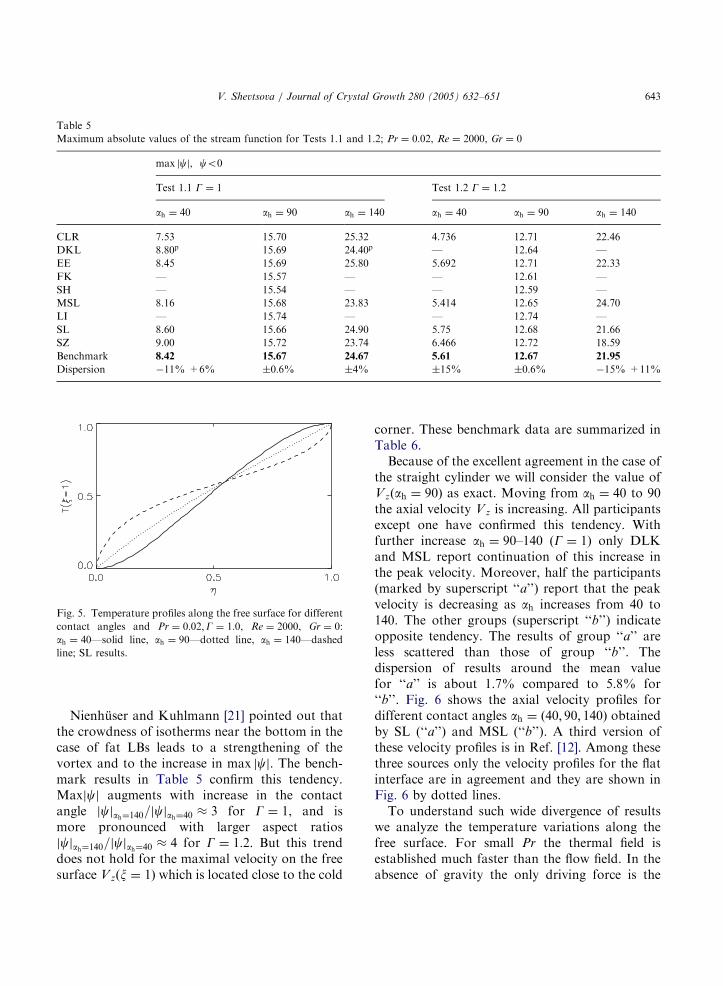
Zero gravity case, Gr ¼ 0: The steady axisym-metric flow patterns in the case of Test 1.1 arepresented in Fig. 4. The isotherms are parallel atthe core part of the LB indicating weak convectionfor small Pr number. They are perpendicular tothe thermally insulated free surface. The center ofthe vorticity is shifted downwards for the slenderLB and moves up with increasing LB volumeapproaching the mid-plane and the streamlinesbecome more circular.The first test compares the values of the stream

function, which is negative, co0. Thus, theabsolute values are placed in the Table 5. Thesuperscript ‘‘p’’ in the case of DKL indicatesresults from Nienhuser [12] coming from the sameschool. The last line shows the benchmark value,which is defined as the mean value for this case ofsmall dispersion of results.

ARTICLE IN PRESS

(a) (b) (c)

Fig. 4. Isotherms (left) and stream lines (right) for the Test 1.1; Pr ¼ 0:02;G ¼ 1:0, Re ¼ 2000, Gr ¼ 0. Different geometries

correspond to (a) ah ¼ 40, (b) ah ¼ 90, (c) ah ¼ 140; SL results.

Table 4

Geometries used in the benchmark tests


For the stream function the best agreement isobtained in the case of straight interface, thescattering of the results does not exceed 1% forboth unit and non-unit aspect ratios. Even in thiscase the results are grid dependent as was shownby two groups, DKL and FK, who performedsuch study. Results with best resolution are placedin Table 5.Note that smaller angles and larger aspect ratios

lead to the largest dispersion in max jcj. In the caseG ¼ 1:0 the dispersion is 3–5% for the fat liquidbridges ah ¼ 140, increasing to 6–11% for theslender ones ah ¼ 40. The situation is worse for

aspect ratio G ¼ 1:2 when the divergence reaches15% for both slender and fat LBs.Temperature profiles for different contact angles

are shown in Fig. 5. The ‘‘S’’— shape of highPrandtl number temperature profiles is not applic-able here. In the case of a plain interface thetemperature profile is close to linear. For smalland large contact angles the temperature profilesbend to opposite sides. In contrast with high Pr

number liquids there is no pronounced spike ofisotherms near the rigid walls. However, with largevolumes ah ¼ 140 the isolines are denser near thecold and hot corners.

ARTICLE IN PRESS

Table 5

Maximum absolute values of the stream function for Tests 1.1 and 1.2; Pr ¼ 0:02, Re ¼ 2000, Gr ¼ 0

max jcj, co0

Test 1.1 G ¼ 1 Test 1.2 G ¼ 1:2

ah ¼ 40 ah ¼ 90 ah ¼ 140 ah ¼ 40 ah ¼ 90 ah ¼ 140

CLR 7.53 15.70 25.32 4.736 12.71 22.46

DKL 8.80p 15.69 24.40p — 12.64 —

EE 8.45 15.69 25.80 5.692 12.71 22.33

FK — 15.57 — — 12.61 —

SH — 15.54 — — 12.59 —

MSL 8.16 15.68 23.83 5.414 12.65 24.70

LI — 15.74 — — 12.74 —

SL 8.60 15.66 24.90 5.75 12.68 21.66

SZ 9.00 15.72 23.74 6.466 12.72 18.59

Benchmark 8.42 15.67 24.67 5.61 12.67 21.95

Dispersion �11% +6% �0:6% �4% �15% �0:6% �15% +11%

Fig. 5. Temperature profiles along the free surface for different

contact angles and Pr ¼ 0:02;G ¼ 1:0, Re ¼ 2000, Gr ¼ 0:

ah ¼ 40—solid line, ah ¼ 90—dotted line, ah ¼ 140—dashed

line; SL results.


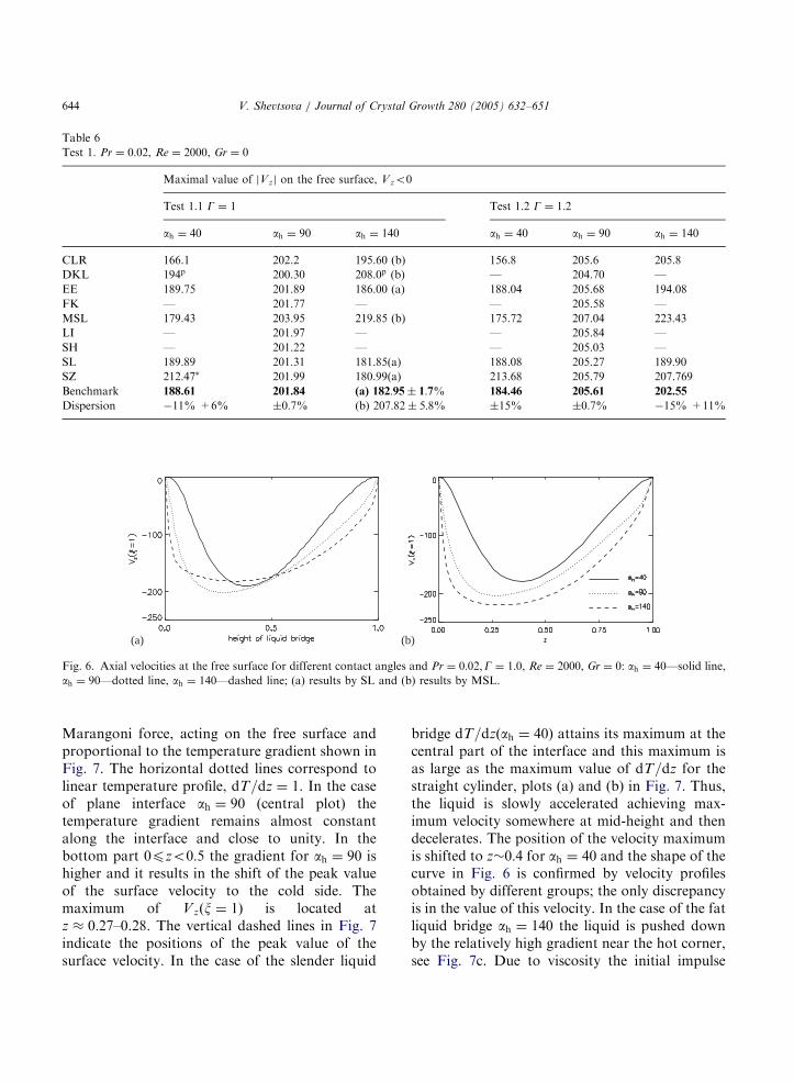
Nienhuser and Kuhlmann [21] pointed out thatthe crowdness of isotherms near the bottom in thecase of fat LBs leads to a strengthening of thevortex and to the increase in max jcj. The bench-mark results in Table 5 confirm this tendency.Maxjcj augments with increase in the contactangle jcjah¼140=jcjah¼40 � 3 for G ¼ 1, and ismore pronounced with larger aspect ratiosjcjah¼140=jcjah¼40 � 4 for G ¼ 1:2. But this trenddoes not hold for the maximal velocity on the freesurface V zðx ¼ 1Þ which is located close to the cold

corner. These benchmark data are summarized inTable 6.Because of the excellent agreement in the case of

the straight cylinder we will consider the value ofVzðah ¼ 90Þ as exact. Moving from ah ¼ 40 to 90the axial velocity Vz is increasing. All participantsexcept one have confirmed this tendency. Withfurther increase ah ¼ 90–140 (G ¼ 1) only DLKand MSL report continuation of this increase inthe peak velocity. Moreover, half the participants(marked by superscript ‘‘a’’) report that the peakvelocity is decreasing as ah increases from 40 to140. The other groups (superscript ‘‘b’’) indicateopposite tendency. The results of group ‘‘a’’ areless scattered than those of group ‘‘b’’. Thedispersion of results around the mean valuefor ‘‘a’’ is about 1.7% compared to 5.8% for‘‘b’’. Fig. 6 shows the axial velocity profiles fordifferent contact angles ah ¼ ð40; 90; 140Þ obtainedby SL (‘‘a’’) and MSL (‘‘b’’). A third version ofthese velocity profiles is in Ref. [12]. Among thesethree sources only the velocity profiles for the flatinterface are in agreement and they are shown inFig. 6 by dotted lines.To understand such wide divergence of results

we analyze the temperature variations along thefree surface. For small Pr the thermal field isestablished much faster than the flow field. In theabsence of gravity the only driving force is the

ARTICLE IN PRESS

Table 6

Test 1. Pr ¼ 0:02, Re ¼ 2000, Gr ¼ 0

Maximal value of jVzj on the free surface, Vzo0

Test 1.1 G ¼ 1 Test 1.2 G ¼ 1:2

ah ¼ 40 ah ¼ 90 ah ¼ 140 ah ¼ 40 ah ¼ 90 ah ¼ 140

CLR 166.1 202.2 195.60 (b) 156.8 205.6 205.8

DKL 194p 200.30 208.0p (b) — 204.70 —

EE 189.75 201.89 186.00 (a) 188.04 205.68 194.08

FK — 201.77 — — 205.58 —

MSL 179.43 203.95 219.85 (b) 175.72 207.04 223:43LI — 201.97 — — 205.84 —

SH — 201.22 — — 205.03 —

SL 189.89 201.31 181.85(a) 188.08 205.27 189:90SZ 212:47� 201.99 180.99(a) 213.68 205.79 207.769

Benchmark 188.61 201.84 (a) 182:95� 1:7% 184.46 205.61 202.55

Dispersion �11% +6% �0:7% (b) 207:82� 5:8% �15% �0:7% �15% +11%

(a) (b)

Fig. 6. Axial velocities at the free surface for different contact angles and Pr ¼ 0:02;G ¼ 1:0, Re ¼ 2000, Gr ¼ 0: ah ¼ 40—solid line,

ah ¼ 90—dotted line, ah ¼ 140—dashed line; (a) results by SL and (b) results by MSL.


Marangoni force, acting on the free surface andproportional to the temperature gradient shown inFig. 7. The horizontal dotted lines correspond tolinear temperature profile, dT=dz ¼ 1. In the caseof plane interface ah ¼ 90 (central plot) thetemperature gradient remains almost constantalong the interface and close to unity. In thebottom part 0pzo0:5 the gradient for ah ¼ 90 ishigher and it results in the shift of the peak valueof the surface velocity to the cold side. Themaximum of Vzðx ¼ 1Þ is located atz � 0:27–0.28. The vertical dashed lines in Fig. 7indicate the positions of the peak value of thesurface velocity. In the case of the slender liquid

bridge dT=dzðah ¼ 40Þ attains its maximum at thecentral part of the interface and this maximum isas large as the maximum value of dT=dz for thestraight cylinder, plots (a) and (b) in Fig. 7. Thus,the liquid is slowly accelerated achieving max-imum velocity somewhere at mid-height and thendecelerates. The position of the velocity maximumis shifted to z 0:4 for ah ¼ 40 and the shape of thecurve in Fig. 6 is confirmed by velocity profilesobtained by different groups; the only discrepancyis in the value of this velocity. In the case of the fatliquid bridge ah ¼ 140 the liquid is pushed downby the relatively high gradient near the hot corner,see Fig. 7c. Due to viscosity the initial impulse

ARTICLE IN PRESS

(a) (b) (c)

Fig. 7. Temperature gradients along the free surface for different contact angles—ah ¼ ð40; 90; 140Þ: Pr ¼ 0:02;G ¼ 1:0, Re ¼ 2000,

Gr ¼ 0; SL results. The vertical dashed lines indicate location of the maximum of Vz and horizontal dotted lines correspond to

dT=dz ¼ 1:

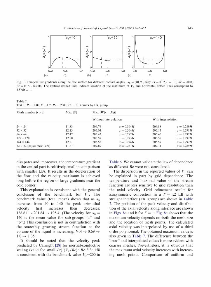
Table 7

Test 1. Pr ¼ 0:02;G ¼ 1:2, Re ¼ 2000, Gr ¼ 0; Results by FK group

Mesh number ðr � zÞ Max jCj Max jW ðr ¼ R0Þj

Without interpolation With interpolation

24� 24 11.83 204.76 z ¼ 0:304H 204.88 z ¼ 0:289H

32� 32 12.13 205.04 z ¼ 0:304H 205.13 z ¼ 0:291H

64� 64 12.47 205.42 z ¼ 0:282H 205.46 z ¼ 0:292H

128� 128 12.60 205.58 z ¼ 0:293H 205.58 z ¼ 0:292H

144� 144 12.61 205.58 z ¼ 0:294H 205.59 z ¼ 0:292H

32� 32 (equal mesh size) 11.67 207.69 z ¼ 0:281H 207.74 z ¼ 0:289H


dissipates and, moreover, the temperature gradientin the central part is relatively small in comparisonwith smaller LBs. It results in the deceleration ofthe flow and the velocity maximum is achievedlong before the region of large gradients near thecold corner.This explanation is consistent with the general

conclusion of the benchmark for V z. Thebenchmark value (total mean) shows that as ahincreases from 40 to 140 the peak azimuthalvelocity first increases then decreases:188:61 ! 201:84 ! 195:4. (The velocity for ah ¼140 is the mean value for sub-groups ‘‘a’’ and‘‘b’’.) This conclusion is not in contradiction withthe smoothly growing stream function as thevolume of the liquid is increasing: Vol ) 0:69 !

1:0 ! 1:35:It should be noted that the velocity peak

predicted by Canright [28] for inertial-conductivescaling (valid for small Pr) ðV z=ReÞ Re�1=3 158is consistent with the benchmark value V z 200 in

Table 6. We cannot validate the law of dependenceas different Re were not considered.The dispersion in the reported values of V z can

be explained in part by grid dependence. Thetemperature and maximal value of the streamfunction are less sensitive to grid resolution thanthe axial velocity. Grid refinement results foraxisymmetric convection in a G ¼ 1:2 LB withstraight interface (FK group) are shown in Table7. The position of the peak velocity and distribu-tion of the axial velocity along interface are shownin Figs. 8a and b for G ¼ 1. Fig. 8a shows that themaximum velocity depends on both the mesh sizeand the location of mesh points. The calculatedaxial velocity was interpolated by use of a thirdorder polynomial. The obtained maximum value isalso given in Table 7. The difference between the‘‘raw’’ and interpolated values is more evident withcoarser meshes. Nevertheless, it is obvious thatthe maximum axial velocity increases with increas-ing mesh points. Comparison of uniform and

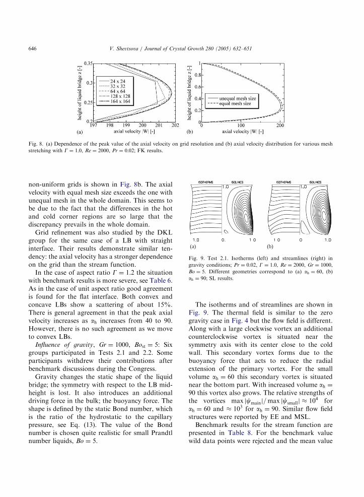
ARTICLE IN PRESS

Fig. 8. (a) Dependence of the peak value of the axial velocity on grid resolution and (b) axial velocity distribution for various mesh

stretching with G ¼ 1:0, Re ¼ 2000, Pr ¼ 0:02; FK results.

(a) (b)

Fig. 9. Test 2.1. Isotherms (left) and streamlines (right) in

gravity conditions; Pr ¼ 0:02, G ¼ 1:0, Re ¼ 2000, Gr ¼ 1000,

Bo ¼ 5. Different geometries correspond to (a) ah ¼ 60, (b)

ah ¼ 90; SL results.


non-uniform grids is shown in Fig. 8b. The axialvelocity with equal mesh size exceeds the one withunequal mesh in the whole domain. This seems tobe due to the fact that the differences in the hotand cold corner regions are so large that thediscrepancy prevails in the whole domain.Grid refinement was also studied by the DKL

group for the same case of a LB with straightinterface. Their results demonstrate similar ten-dency: the axial velocity has a stronger dependenceon the grid than the stream function.In the case of aspect ratio G ¼ 1:2 the situation

with benchmark results is more severe, see Table 6.As in the case of unit aspect ratio good agreementis found for the flat interface. Both convex andconcave LBs show a scattering of about 15%.There is general agreement in that the peak axialvelocity increases as ah increases from 40 to 90.However, there is no such agreement as we moveto convex LBs.

Influence of gravity, Gr ¼ 1000, Bost ¼ 5: Sixgroups participated in Tests 2.1 and 2.2. Someparticipants withdrew their contributions afterbenchmark discussions during the Congress.Gravity changes the static shape of the liquid

bridge; the symmetry with respect to the LB mid-height is lost. It also introduces an additionaldriving force in the bulk; the buoyancy force. Theshape is defined by the static Bond number, whichis the ratio of the hydrostatic to the capillarypressure, see Eq. (13). The value of the Bondnumber is chosen quite realistic for small Prandtlnumber liquids, Bo ¼ 5.

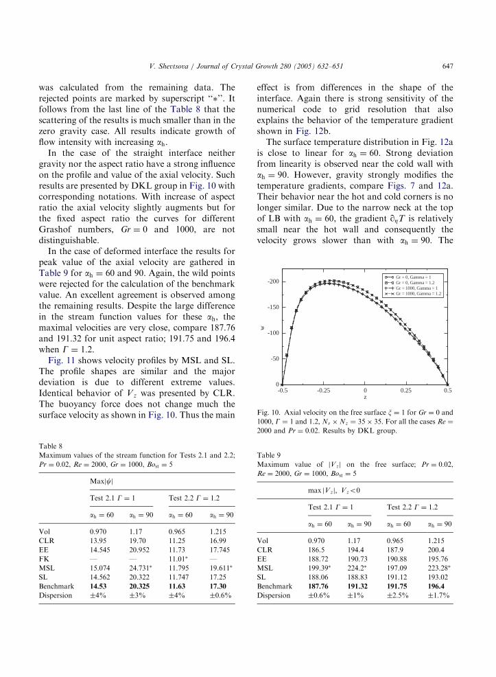
The isotherms and of streamlines are shown inFig. 9. The thermal field is similar to the zerogravity case in Fig. 4 but the flow field is different.Along with a large clockwise vortex an additionalcounterclockwise vortex is situated near thesymmetry axis with its center close to the coldwall. This secondary vortex forms due to thebuoyancy force that acts to reduce the radialextension of the primary vortex. For the smallvolume ah ¼ 60 this secondary vortex is situatednear the bottom part. With increased volume ah ¼90 this vortex also grows. The relative strengths ofthe vortices max jcmainj=max jcsmallj � 104 forah ¼ 60 and � 103 for ah ¼ 90. Similar flow fieldstructures were reported by EE and MSL.Benchmark results for the stream function are

presented in Table 8. For the benchmark valuewild data points were rejected and the mean value

ARTICLE IN PRESS

-0.5 -0.25 0 0.25 0.5z

-200

-150

-100

-50

0

w

Gr = 0, Gamma = 1Gr = 0, Gamma = 1.2Gr = 1000, Gamma = 1Gr = 1000, Gamma = 1.2

Fig. 10. Axial velocity on the free surface x ¼ 1 for Gr ¼ 0 and

1000, G ¼ 1 and 1.2, N � N ¼ 35� 35. For all the cases Re ¼


was calculated from the remaining data. Therejected points are marked by superscript ‘‘�’’. Itfollows from the last line of the Table 8 that thescattering of the results is much smaller than in thezero gravity case. All results indicate growth offlow intensity with increasing ah.In the case of the straight interface neither

gravity nor the aspect ratio have a strong influenceon the profile and value of the axial velocity. Suchresults are presented by DKL group in Fig. 10 withcorresponding notations. With increase of aspectratio the axial velocity slightly augments but forthe fixed aspect ratio the curves for differentGrashof numbers, Gr ¼ 0 and 1000, are notdistinguishable.In the case of deformed interface the results for

peak value of the axial velocity are gathered inTable 9 for ah ¼ 60 and 90. Again, the wild pointswere rejected for the calculation of the benchmarkvalue. An excellent agreement is observed amongthe remaining results. Despite the large differencein the stream function values for these ah, themaximal velocities are very close, compare 187:76and 191:32 for unit aspect ratio; 191:75 and 196:4when G ¼ 1:2.Fig. 11 shows velocity profiles by MSL and SL.

The profile shapes are similar and the majordeviation is due to different extreme values.Identical behavior of Vz was presented by CLR.The buoyancy force does not change much thesurface velocity as shown in Fig. 10. Thus the main

Table 8

Maximum values of the stream function for Tests 2.1 and 2.2;

Pr ¼ 0:02, Re ¼ 2000, Gr ¼ 1000, Bost ¼ 5

Maxjcj

Test 2.1 G ¼ 1 Test 2.2 G ¼ 1:2

ah ¼ 60 ah ¼ 90 ah ¼ 60 ah ¼ 90

Vol 0.970 1.17 0.965 1.215

CLR 13.95 19.70 11.25 16.99

EE 14.545 20.952 11.73 17.745

FK — — 11.01� —

MSL 15.074 24.731� 11.795 19.611�

SL 14.562 20.322 11.747 17.25

Benchmark 14.53 20.325 11.63 17.30

Dispersion �4% �3% �4% �0:6%

effect is from differences in the shape of theinterface. Again there is strong sensitivity of thenumerical code to grid resolution that alsoexplains the behavior of the temperature gradientshown in Fig. 12b.The surface temperature distribution in Fig. 12a

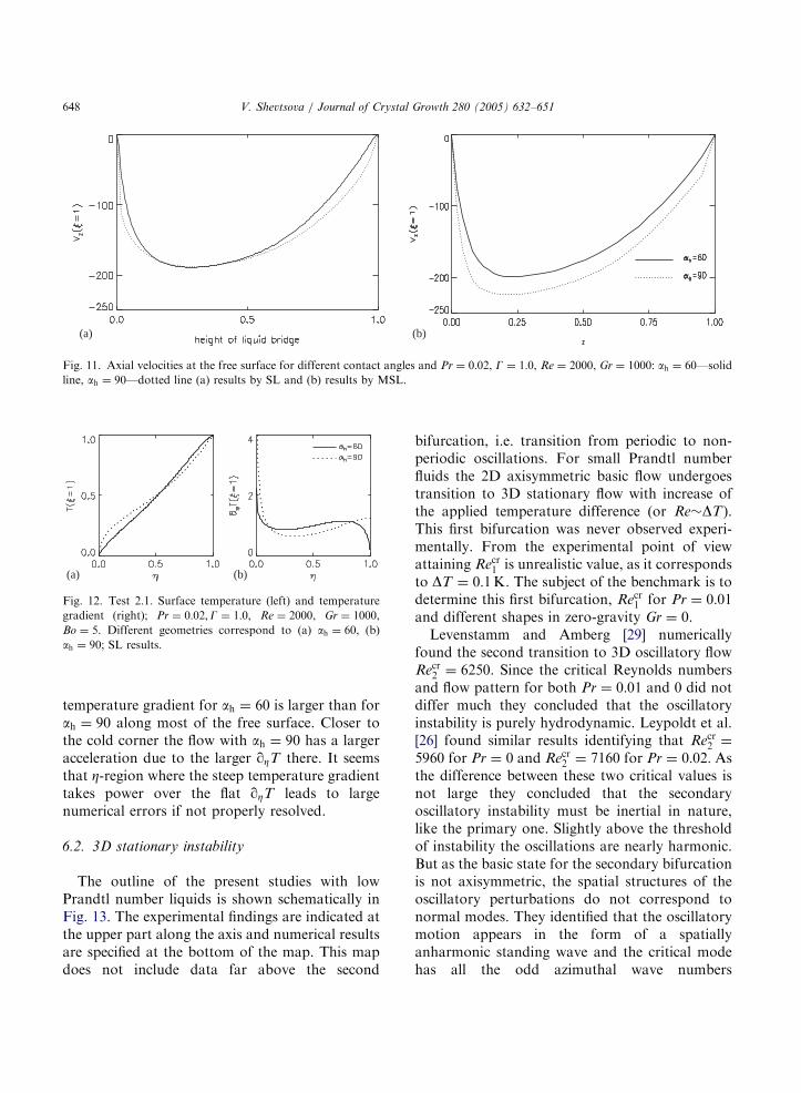
is close to linear for ah ¼ 60. Strong deviationfrom linearity is observed near the cold wall withah ¼ 90. However, gravity strongly modifies thetemperature gradients, compare Figs. 7 and 12a.Their behavior near the hot and cold corners is nolonger similar. Due to the narrow neck at the topof LB with ah ¼ 60, the gradient qZT is relativelysmall near the hot wall and consequently thevelocity grows slower than with ah ¼ 90: The

r z

2000 and Pr ¼ 0:02. Results by DKL group.

Table 9

Maximum value of jV zj on the free surface; Pr ¼ 0:02,Re ¼ 2000, Gr ¼ 1000, Bost ¼ 5

max jV zj; Vzo0

Test 2.1 G ¼ 1 Test 2.2 G ¼ 1:2

ah ¼ 60 ah ¼ 90 ah ¼ 60 ah ¼ 90

Vol 0.970 1.17 0.965 1.215

CLR 186.5 194.4 187.9 200.4

EE 188.72 190.73 190.88 195.76

MSL 199.39� 224.2� 197.09 223.28�

SL 188.06 188.83 191.12 193.02

Benchmark 187.76 191.32 191.75 196.4

Dispersion �0:6% �1% �2:5% �1:7%

ARTICLE IN PRESS

(a) (b)

Fig. 11. Axial velocities at the free surface for different contact angles and Pr ¼ 0:02, G ¼ 1:0, Re ¼ 2000, Gr ¼ 1000: ah ¼ 60—solid

line, ah ¼ 90—dotted line (a) results by SL and (b) results by MSL.

(a) (b)

Fig. 12. Test 2.1. Surface temperature (left) and temperature

gradient (right); Pr ¼ 0:02;G ¼ 1:0, Re ¼ 2000, Gr ¼ 1000,

Bo ¼ 5. Different geometries correspond to (a) ah ¼ 60, (b)

ah ¼ 90; SL results.


temperature gradient for ah ¼ 60 is larger than forah ¼ 90 along most of the free surface. Closer tothe cold corner the flow with ah ¼ 90 has a largeracceleration due to the larger qZT there. It seemsthat Z-region where the steep temperature gradienttakes power over the flat qZT leads to largenumerical errors if not properly resolved.

6.2. 3D stationary instability

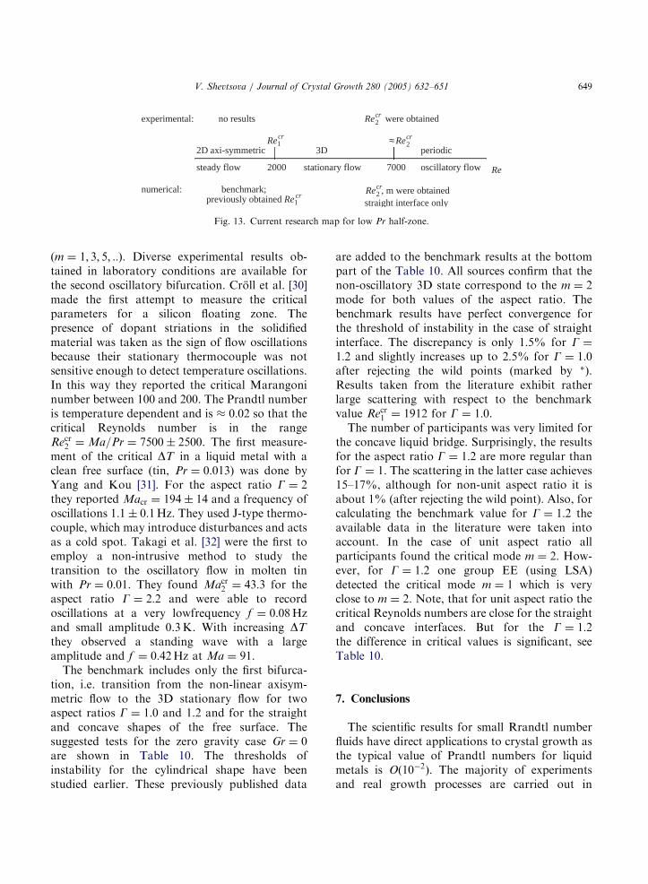
The outline of the present studies with lowPrandtl number liquids is shown schematically inFig. 13. The experimental findings are indicated atthe upper part along the axis and numerical resultsare specified at the bottom of the map. This mapdoes not include data far above the second

bifurcation, i.e. transition from periodic to non-periodic oscillations. For small Prandtl numberfluids the 2D axisymmetric basic flow undergoestransition to 3D stationary flow with increase ofthe applied temperature difference (or Re DT).This first bifurcation was never observed experi-mentally. From the experimental point of viewattaining Recr1 is unrealistic value, as it correspondsto DT ¼ 0:1K. The subject of the benchmark is todetermine this first bifurcation, Recr1 for Pr ¼ 0:01and different shapes in zero-gravity Gr ¼ 0.Levenstamm and Amberg [29] numerically

found the second transition to 3D oscillatory flowRecr2 ¼ 6250. Since the critical Reynolds numbersand flow pattern for both Pr ¼ 0:01 and 0 did notdiffer much they concluded that the oscillatoryinstability is purely hydrodynamic. Leypoldt et al.[26] found similar results identifying that Recr2 ¼

5960 for Pr ¼ 0 and Recr2 ¼ 7160 for Pr ¼ 0:02: Asthe difference between these two critical values isnot large they concluded that the secondaryoscillatory instability must be inertial in nature,like the primary one. Slightly above the thresholdof instability the oscillations are nearly harmonic.But as the basic state for the secondary bifurcationis not axisymmetric, the spatial structures of theoscillatory perturbations do not correspond tonormal modes. They identified that the oscillatorymotion appears in the form of a spatiallyanharmonic standing wave and the critical modehas all the odd azimuthal wave numbers

ARTICLE IN PRESS

experimental: no results

numerical: benchmark;previously obtained Re1

cr

Re2000

Re1cr

2D axi-symmetric

steady flow

3D

stationary flow 7000

≈

Re2 were obtained

, m were obtainedstraight interface only

periodic

oscillatory flow

cr

Re2cr

Re2cr

Fig. 13. Current research map for low Pr half-zone.


ðm ¼ 1; 3; 5; ::Þ. Diverse experimental results ob-tained in laboratory conditions are available forthe second oscillatory bifurcation. Croll et al. [30]made the first attempt to measure the criticalparameters for a silicon floating zone. Thepresence of dopant striations in the solidifiedmaterial was taken as the sign of flow oscillationsbecause their stationary thermocouple was notsensitive enough to detect temperature oscillations.In this way they reported the critical Marangoninumber between 100 and 200. The Prandtl numberis temperature dependent and is � 0:02 so that thecritical Reynolds number is in the rangeRecr2 ¼ Ma=Pr ¼ 7500� 2500. The first measure-ment of the critical DT in a liquid metal with aclean free surface (tin, Pr ¼ 0:013) was done byYang and Kou [31]. For the aspect ratio G ¼ 2they reported Macr ¼ 194� 14 and a frequency ofoscillations 1:1� 0:1Hz. They used J-type thermo-couple, which may introduce disturbances and actsas a cold spot. Takagi et al. [32] were the first toemploy a non-intrusive method to study thetransition to the oscillatory flow in molten tinwith Pr ¼ 0:01. They found Macr2 ¼ 43:3 for theaspect ratio G ¼ 2:2 and were able to recordoscillations at a very lowfrequency f ¼ 0:08Hzand small amplitude 0.3K. With increasing DT

they observed a standing wave with a largeamplitude and f ¼ 0:42Hz at Ma ¼ 91.The benchmark includes only the first bifurca-

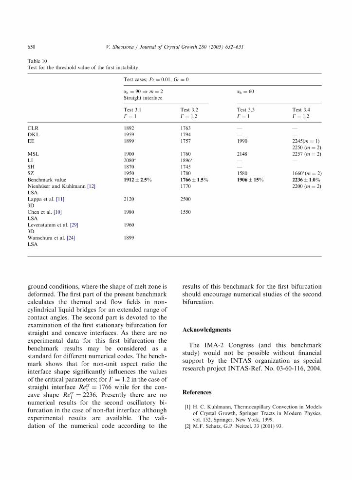
tion, i.e. transition from the non-linear axisym-metric flow to the 3D stationary flow for twoaspect ratios G ¼ 1:0 and 1.2 and for the straightand concave shapes of the free surface. Thesuggested tests for the zero gravity case Gr ¼ 0are shown in Table 10. The thresholds ofinstability for the cylindrical shape have beenstudied earlier. These previously published data

are added to the benchmark results at the bottompart of the Table 10. All sources confirm that thenon-oscillatory 3D state correspond to the m ¼ 2mode for both values of the aspect ratio. Thebenchmark results have perfect convergence forthe threshold of instability in the case of straightinterface. The discrepancy is only 1:5% for G ¼

1:2 and slightly increases up to 2:5% for G ¼ 1:0after rejecting the wild points (marked by �).Results taken from the literature exhibit ratherlarge scattering with respect to the benchmarkvalue Recr1 ¼ 1912 for G ¼ 1:0.The number of participants was very limited for

the concave liquid bridge. Surprisingly, the resultsfor the aspect ratio G ¼ 1:2 are more regular thanfor G ¼ 1. The scattering in the latter case achieves15–17%, although for non-unit aspect ratio it isabout 1% (after rejecting the wild point). Also, forcalculating the benchmark value for G ¼ 1:2 theavailable data in the literature were taken intoaccount. In the case of unit aspect ratio allparticipants found the critical mode m ¼ 2. How-ever, for G ¼ 1:2 one group EE (using LSA)detected the critical mode m ¼ 1 which is veryclose to m ¼ 2. Note, that for unit aspect ratio thecritical Reynolds numbers are close for the straightand concave interfaces. But for the G ¼ 1:2the difference in critical values is significant, seeTable 10.

7. Conclusions

The scientific results for small Rrandtl numberfluids have direct applications to crystal growth asthe typical value of Prandtl numbers for liquidmetals is Oð10�2Þ. The majority of experimentsand real growth processes are carried out in

ARTICLE IN PRESS

Table 10

Test for the threshold value of the first instability

Test cases; Pr ¼ 0:01, Gr ¼ 0

ah ¼ 90 ) m ¼ 2 ah ¼ 60

Straight interface

Test 3.1 Test 3.2 Test 3.3 Test 3.4

G ¼ 1 G ¼ 1:2 G ¼ 1 G ¼ 1:2

CLR 1892 1763 — —

DKL 1959 1794 — —

EE 1899 1757 1990 2245ðm ¼ 1Þ

2250 ðm ¼ 2Þ

MSL 1900 1760 2148 2257 ðm ¼ 2Þ

LI 2080� 1896� — —

SH 1870 1745 —

SZ 1950 1780 1580 1660�ðm ¼ 2Þ

Benchmark value 1912� 2:5% 1766� 1:5% 1906� 15% 2236� 1:0%Nienhuser and Kuhlmann [12] 1770 2200 ðm ¼ 2Þ

LSA

Lappa et al. [11] 2120 2500

3D

Chen et al. [10] 1980 1550

LSA

Levenstamm et al. [29] 1960

3D

Wanschura et al. [24] 1899

LSA


ground conditions, where the shape of melt zone isdeformed. The first part of the present benchmarkcalculates the thermal and flow fields in non-cylindrical liquid bridges for an extended range ofcontact angles. The second part is devoted to theexamination of the first stationary bifurcation forstraight and concave interfaces. As there are noexperimental data for this first bifurcation thebenchmark results may be considered as astandard for different numerical codes. The bench-mark shows that for non-unit aspect ratio theinterface shape significantly influences the valuesof the critical parameters; for G ¼ 1:2 in the case ofstraight interface Recr1 ¼ 1766 while for the con-cave shape Recr1 ¼ 2236: Presently there are nonumerical results for the second oscillatory bi-furcation in the case of non-flat interface althoughexperimental results are available. The vali-dation of the numerical code according to the

results of this benchmark for the first bifurcationshould encourage numerical studies of the secondbifurcation.

Acknowledgments

The IMA-2 Congress (and this benchmarkstudy) would not be possible without financialsupport by the INTAS organization as specialresearch project INTAS-Ref. No. 03-60-116, 2004.

References

[1] H. C. Kuhlmann, Thermocapillary Convection in Models

of Crystal Growth, Springer Tracts in Modern Physics,

vol. 152, Springer, New York, 1999.

[2] M.F. Schatz, G.P. Neitzel, 33 (2001) 93.

ARTICLE IN PRESS


[3] D. Schwabe, R. Velten, A. Scharmann, J. Crystal Growth

99 (1990) 1258.

[4] L. Carotenuto, D. Castagnolo, C. Albanese, R. Monti,

Phys. Fluids 10 (1997) 555.

[5] Zh. Kozhoukharova, S. Slavchev, J. Crystal Growth 74

(1986) 236.

[6] V.M. Shevtsova, H.C. Kuhlmann, H.J. Rath, in: L. Ratke,

H. Walter, B. Feuerbacher (Eds.), LNP, Materials

and Fluids Under Low Gravity, Springer, Berlin, 1995,

pp. 323–329.

[7] H.C. Kuhlmann, C. Nienhuser, H.J. Rath, J. Eng. Math.

36 (1999) 207.

[8] V.M. Shevtsova, J.C. Legros, Phys. Fluids 10 (1998) 1621.

[9] Q.S. Chen, W.R. Hu, Int. J. Heat Mass Transfer 42 (1998)

825.

[10] Q.S. Chen, W.R. Hu, V. Prasad, J. Crystal Growth 203

(1999) 261.

[11] M. Lappa, R. Savino, R. Monti, Int. J. Heat Mass

Transfer 44 (2001) 1983.

[12] C. Nienhuser, H.C. Kuhlmann, J. Fluid Mech. 458 (2002)

35.

[13] C. Nienhuser, H.C. Kuhlmann, J. Fluid Mech. 480 (2003)

333.

[14] L.B.S. Sumner, G.P. Neitzel, Phys. Fluids 13 (2001) 107.

[15] Z.M. Tang, W.R. Hu, N. Imaishi, Int. J. Heat Mass

Transfer 44 (2001) 1299.

[16] B.C. Sim, A. Zebib, AIAA J. Thermophys. Heat transfer

16 (2002a) 553.

[17] M.K. Ermakov, M.S. Ermakova, J. Crystal Growth 266

(2004) 160.

[18] Y. Kamotani, S. Ostrach, J. Masud, J. Fluid Mech. 410

(2000) 211.

[19] B.-C. Sim, A. Zebib, Int. J. Heat Mass Transfer 45 (2002b)

4983.

[20] V.M. Shevtsova, M.K. Ermakov, E. Ryabitskii, J.C.

Legros, Acta Astonautica 41 (1997) 471.

[21] H.C. Kuhlmann, C. Nienhuser, Fluid Dynamic Res. 31

(2002) 103.

[22] M.R. Mundrane, A. Zebib, AIAA J. Thermophys. Heat

Transfer 9 (1995) 795.

[23] V.M. Shevtsova, D.E. Melnikov, J.C. Legros, Phys. Fluids

13 (2001) 2851.

[24] M. Wanschura, V.M. Shevtsova, H.C. Kuhlmann, H.J.

Rath, Phys. Fluids 5 (1995) 912.

[25] G. Chen Lizee, B. Roux, J. Crystal Growth 180 (1997) 638.

[26] J. Leypoldt, H.C. Kuhlmann, H.J. Rath, J. Fluid Mech.

414 (2000) 285.

[27] H. Ozoe, K. Toh, J. Crystal Growth 130 (1993) 645.

[28] D. Canright, Phys. Fluids 6 (1994) 1415.

[29] M. Levenstam, G. Amberg, J. Fluid Mech. 297 (1995) 357.

[30] A. Croll, W. Muller-Sebert, K.W. Benz, R. Nitsche,

Microgravity Sci. Tehcnol. III/4 (1991) 204.

[31] Y.K. Yang, S. Kou, J. Crystal Growth 222 (2001) 135.

[32] K. Takagi, M. Otaka, H. Natsui, T. Arai, S. Yoda, Z.

Yuan, K. Mukai, S. Yasuhiro, N. Imaishi, J. Crystal

Growth 233 (2001) 399.

Documents

Thermalconvectioninliquidbridgeswithcurvedfreesurfaces ...homepages.ulb.ac.be/~dmelniko/Papers/Journal_of_Crystal...Benchmarkofnumericalsolutions ValentinaShevtsova MRC, CP-165/62,