Embed Size (px)
Citation preview

THERMAL-FLOW CODE FOR MODELING GAS DYNAMICS AND HEAT TRANSFERIN SPACE SHUTTLE SOLID ROCKET MOTOR JOINTS
Qunzhen Wang*, Edward C. Mathias t, Joe R. Heman _ and Cory W. Smith*
Thiokol Propulsion, Cordant Technologies Inc.
P.O. Box 707, M/S 252, Brigham City, UT 84302
INTRODUCTION
It is important to accurately predict the pressure,
temperature, as well as the amount of O-ring erosion in
the space shuttle Reusable Solid Rocket Motor(RSRM) joints in the event of a leak path. The
scenarios considered are typically hot combustion gas
rapid pressurization events of small volumes throughnarrow, restricted flow paths. The ideal method for this
prediction is a transient three-dimensional
computational fluid dynamics calculation withcomputational domain including both the combustion
gas and the surrounding solid regions. However, this
has not yet been demonstrated to be economical for this
application due to the enormous amount of computertime and memory required. Consequently, all CFD
applications in RSRM joints t2 are steady-statesimulations with solid regions being excluded from the
computational domain by either assuming a constant
wall temperature or assuming no heat transfer betweenthe hot combustion gas and cool solid walls.
Currently there are two computer codes, known to theauthors, available to model the gas dynamics, heat
transfer, and O-ring erosion in the RSRM joint
pressurization process. One is ORING2 36, which wasdeveloped at Thioko[ Propulsion, and the other is JPR 7,
which was developed at NASA Marshall Space Flight
Center. A way to improve the current prediction
technique is to modify the transient compressible flowcalculation since the pressure, temperature, and
velocity of the combustion gas are not calculated from
the time-dependent Navier-Stokes equations. Instead.
some empirical correlations are used to predict the gas
temperature, mass flow rate, and other flow properties
by assuming a quasi-steady state flow in a constantcross-section area pipe (i.e., there is no grid in the
paths). Furthermore, ORING2 can only handleconfigurations with two volumes and two paths while it
takes significant coding for JPR to do complicated
configurations with more than two volumes.
A new thermal-flow simulation code, called SFLOW,
has been developed to model the gas dynamics, heattransfer, as well as O-ring and flow path erosion inside
the space shuttle RSRM joints. The details arediscussed in this paper. The SFLOW methodologyeliminates some of the approximations inherent in other
simulation and prediction tools. This is accomplished
by combining SINDA/G ® (Network Analysis, Inc.8), acommercial thermal analyzer, and SHARP ®9t4, a
general-purpose CFD code developed at Thiokol
Propulsion. The pressure, temperature, and velocity ofthe combustion gas in the leak paths are calculated in
SHARP" by solving the time-dependent Navier-Stokes
equations while the heat conduction in the solid is
modeled by SINDA/G ®. The two codes are coupled bythe heat transfer at the solid-gas interface. The number
of flow paths and volumes in SFLOW is limited only
by the memory of the computer used to run SFLOW.
Although SHARP * can solve one-dimensional, two-dimensionaL, as well as three-dimensional flow
problems, the flow inside paths is assumed to be one-dimensional in the current version of SFLOW to reduce
the CPU time and memory requirements. This is a
reasonable approximation due to the fact that leak pathsare usually narrow. The solid in SFLOW, however, canbe one-dimensional, two-dimensional, as well as three-dimensional since it is not always a good
approximation to assume the heat conduction in thesolid region is one-dimensional, especially when thewall material is metal. This is feasible in terms of CPU
time and memory because there is only one equation
(i.e., conservation of energy) to solve in the solid
region compared to five equations (i.e., conservation ofmass, momentum, and energy) needed in the gas regionif the flow is modeled as three-dimensional.
Furthermore, a larger time step can be used in the solidcalculation than that used in the gas calculation since
the solid temperature usually changes much slower than
the flow properties.
Copyright © 2000, Thiokol Propulsion, a Divisionof Cordant Technolgies Inc.Published by the Amencan Institute of Aeronautics and Astronautics, Inc., with permission.
*Principal Engineer, Gas Dynamics, AIAA membert Principal Engineer,HeatTransfer, AIAA memberSSeniorEngineeer, Heat Transfer 1
AmericanInstitute of Aeronautics and Astronautics
https://ntrs.nasa.gov/search.jsp?R=20000065640 2018-06-04T01:38:05+00:00Z

The SHARP® mainprogramis convertedinto asubroutinesothatit canbecalledfromSINDA/G_.Theinputfor thissubroutineincludestheheatfluxfromgastowall,frictionfactoroftheflowpath,massadditionduetoerosion,gasproperties,grid,aswellasboundaryandinitialconditionswhiletheoutputis thepressure,temperature,andvelocityof thegasforeachflowcellataspecifictimestep.In SFLOW,theflowcalculation(i.e.,SHARP®) andthesolidcalculation(i.e.,SINDA/G®)aredecoupledfromeachothersuchthatasmallertimestepcanbeappliedinSHARP®thanthatusedinSINDA/G®.Furthermore,SHARP'*canusemorecellsfortheflowsolutionthanthenumberpassedfromSINDA/G®solidsurfaces.
As a general-purposeCFDcode,SHARPe doesnothavethefrictiontermin thegoverningequationssinceit is typicallyusedfor two-dimensionalandthree-dimensionalflow simulationswherethe frictionisimplicitlytakenintoaccountbytheviscousforceintheresolvednear-wallregionorbyawallfunction.In one-dimensionalflows,however,thefrictiontermhastobeexplicitlyaddeddueto the fact that the velocitygradientin thewall-normaldirectiondoesnotexist.Similarly,aheattransfertermisaddedtotheSHARP_¢equationsbecausethethermalboundarylayeris notsimulatedinSFLOW.Moreover,amassadditiontermis addedin SHARP_ sincetheerosionof thewallmaterialwill generatemass.Finally,minorlosstermssuchasthosedueto suddenexpansionor contractionand flow directionchangeare accountedfor byspecifyingalosscoefficientintheSFLOWinputfileattheappropriateflowcells.The detailsof the solutionscheme,includingthemodelingof gasdynamics,heattransfer,aswellasO-ringandpatherosion,arediscussedin thenextsection,followedby comparisonof SFLOWpredictionstoexactsolutionsor experimentaldata.ThetestcasesincludedFannoflow wherefriction is important,Rayleighflow whereheattransferbetweengasandsolidis important,flowwithmassadditiondueto theerosionof thesolidwall, transientvolumeventingprocess,aswell as sometransientone-dimensionalflowswithanalyticalsolutionsderivedby CaitS.Inaddition,SFLOWhasbeenappliedtomodeltheRSRMnozzlejoint4 subscalehot-flowtests_6,whichsimulateflowsto the primaryandsecondaryO-rings.Thepredictedpressure,temperature(bothgasandsolid),andO-ringerosionfromSFLOWarecomparedwiththemeasureddatainthispaper.
GAS DYNAMICS AND THERMAL
MODELING
GAS DYNAMICS MODELING
In SFLOW, the gas can be either in a flow path or avolume (i.e., cavity), which are treated very differently.
The gas in a volume is assumed to be in quasi-
equilibrium with uniform pressure, temperature, and no
velocity whereas that in a path is solved from the first
principles (i.e., conservation of mass, momentum and
energy).
Gas flow in paths
The transient compressible flow in a path is modeled
using SHARP ®, which is a general-purpose CFD code.
SHARP ® solves the Reynolds averaged Navier-Stokes
equations in one-dimensional form as
a(E,-E,)_c-)Q, S (1)@t ,3x
where the unknowns are
Q=A u (2)
In equation (2), A is the cross-section area, which is a
function of both space x and time t, and/9 and u are
the Reynolds averaged density and velocity,
respectively. The total energy is
)where T is the Reynolds averaged temperature and c v
is the specific heat at constant volume. The inviscid
flux term is given by
E, =A pu"+p (4)
L(e+P).J
while the viscous term is
[° 1Ev = A r_ (5)
ltrll +qtJ
2
American Institute of Aeronautics and Astronautics

The total stress and heat flux include both laminar parts
and turbulence parts as
rll = 2 (p L+// ;)x (6)
I _/, //r )_Tq,=- (y_t)prt " F(y-i_pr r _ (7)
where _ '- and pr _-are the laminar viscosity and Prandtl
number while Pr r is the turbulent Prandtl number. The
turbulent viscosity /.t r is zero for laminar flow while it
is obtained by the widely used k-£ model for
turbulent flow. The source term in equation (1) is
S _
rn
2 _ "2 ax-8 fD,,p I O(KApu:)
1 a(KAp t, _Ir
-O-8JD"PI'¢ 2 ax
(8)
where tn is the mass addition rate due to path erosion,f
is the Darcy friction factor, Dh is the hydraulic diameter
of the path, K is the minor loss coefficient and q is the
heat transfer rate per unit volume from the gas to the
solid wall. The boundary conditions for the pathflowfield are obtained from the pressure and
temperature of the volumes. A path has to be connectedwith a volume at one end; the other end can be
connected to a volume or a solid wall, which could be
either adiabatic or conducting heat away to the solid
region.
Note that, similar to other general-purpose CFD codes,SHARP ® does not have the friction term shown in
equation (8) since it is typically used for 2D and 3Dflow simulations where the friction is implicitly taken
into account by the viscous force in the resolved near-
wall region or by the wall function applied. In one-dimensional flows, however, the friction term has to be
explicitly accounted for due to the fact that the velocity
gradient _u/_ydoes not exist. Similarly, the heat
transfer term in equation (8) is added to SHARP ® due
to the fact that the thermal boundary layer is notsimulated in SFLOW. The mass addition terms are also
added since the erosion or decomposition of the walls
will generate this effect. Finally, minor loss terms suchas those due to sudden expansion or contraction and
turns or bends in the flow path are added in equation
(8).
Friction factor in the flow paths
The friction factor in equation (8) is obtained from the
empirical correlation of Idelchik 17, which depends on
both the shape of the path (i.e., circular, rectangular, or
triangular) and whether the flow is laminar, turbulent,or in transition.
According to Idelchik 17, the gas flow is divided into
laminar, turbulent, and transitional regimes depending
on the cutoff Reynolds numbers defined as
Re,, = 754 exp(0.0065D_, /e) (9)
- .I)11635
Re. = 20900exp(--_-)
(10)
(11)
where £ is the roughness of the flow path. The flow is
laminar if the Reynolds number is below R%, turbulent
if the Reynolds number is above Re¢ , and in the
transitional regime if the Reynolds number is betweenR% and R%. If there are two transitional zones, R% isused to determine which of the two zones the flow is in.
The friction factor in the flow path is then determined
based on the flow Reynolds number as:
• for Re < Re,,
• lbr Re, < Re < Re_,
64f =-- (12)
Re
p( - 0.00275e ) (13)f = 4.4 Re -°'s_ ex D h i
for Re_, < Re < Re
f= 0.145 _ -vat exp(-O.I)Ol7:(Re-Re):)+V,t (14)
Val =0.758-0.0109( f-- ]4,.:.6 (15)
Lo,,)
• for Re > Re
g{ E 2.51"]t-: --_2,o + J
• for Re, < Re < Re, and Re h _<Re, there
one transitional zone
16)
is only
American Institute of Aeronautics and Astronautics

f = (7.244Re -_'_- 0.32)exp (17)
(-0.00172(Re - Re)2)+ 0.032
Pressure and temperature in volumes
Once the flowfield in the path is solved by SHARP ®,
the pressure and temperature in the volumes can beobtained from mass conservation
_- (m) = rh, + Erh (18)
and energy conservation
_(mcJ)= Eri, h-O (19)
where the summation is for all paths which connect to
this volume, thand h are the mass flow rate and
enthalpy at the end of the path, th e is the rate of mass
addition to the gas due to surface erosion, Q is the heat
transfer rate from the gas to the solid boundary whichincludes the convective heat transfer as well as the heattransfer due to erosion, m, P, and T are the mass,
pressure and temperature of the gas in this volume,
respectively. In addition to equations (18) and (19), the
ideal gas law
pV = mRT (20)
where V is the volume of the cavity, was used to solve
the pressure p, temperature T, and mass m of thevolume.
HEAT TRANSFER MODELING
The convective heat transfer between the gas and the
solid wall is modeled as
q=hA (T -T_) (21)
where h is the heat transfer coefficient, A, is the
surface area, T_ and T_, are the temperature of the gas
and solid wall, respectively. This heat transfer rate isused in both SHARP ® and SINDA/G ® so that the total
energy in the system is conserved.
Heat transfer in paths
The heat transfer coefficient in flow paths can be
obtained from the Nusselt number as
kh = N, D (22)
where k is the thermal conductivity. The Nusselt
number depends on both the cross-section shape of the
path and the flow regime. If the flow is laminar and the
path is circular
N,, =4.36 (23)
while for rectangular paths
N = i. 18135 + 2.30595P 'a'3245 (24)
where
6 max(a'b)lr=min 1 ,_j (25)
with a and b being the width and height. For turbulentflow, the Nusselt number is calculated using the
following empirical correlation
SPrRe (#,)°"
N, = ,nax(f,r,.,,.(l.O7_12.Vut./.18(nr,,,_l)))[-_"_j (26)
where f is the friction factor calculated from equation
(12) through (17), and ,t/B and ,//w are the viscosity
evaluated at the average gas temperature and wall
temperature, respectively. In the transitional regime, alinear interpolation between the laminar and turbulent
Nusselt number is applied.
Jet impingement heat transfer
The jet impingement heat transfer correlation used inSFLOW is the same as that in ORING2 and JPR, which
depends on the standoff distance to diameter ratio aswell as whether the flow is laminar, turbulent, or in the
transitional regime. The heat transfer coefficient isobtained fi'om the Stanton number as
thh = S, cr,- (27)
A
If the flow is laminar, the Stanton number is
iS, : 0.763Pr"'_ _ee[,-_---,,, ) (28)
where the Reynolds number Re is calculated at the jet
exit, T_ is the gas temperature at the jet exit, and Tw isthe temperature of the wall surface. For turbulent flowwith a standoff distance to jet diameter ratio L ! D < 2.6
V _ xl/6,F¢T,S, = 0.763Pr -_'" _Wt _-)
(29)
while for LID > 2.6
AmericanInstitute of Aeronautics and Astronautics

s, =0442r'r l +----T--jV-V/T/C (30)
where Le is the Lewis number. The velocity gradient in
the above equations is
V_r,,, = I (31)
tbr L/D < 3.4,
V,r,,, =1-0.196 L� 34 (32)
for 3.4<L/D<8.4,and
ggrad _
( -' I1-exp 0.2315L/ D-0.74
O.13L/ D-0.39(33)
for L / D > 8.4. If the flow is in transitional regime, the
heat transfer coefficient is obtained by linear
interpolation between laminar and turbulent regimes.
Heat transfer in volumes
The heat transfer from the gas in a volume to the solid
boundary can be modeled in four different ways
• Using the impingement jet heat transfer correlationdescribed above
• Using the heat transfer coefficient in the pathsconnected to this volume
• Using a conduction length as h=k/l
• Using a user-specified heat transfer coefficient
The user of SFLOW specifies which of these methods
should be applied to calculate heat transfer coefficienttbr all the gas-solid interfaces in all volumes.
EROSION MODELING
The erosion model used in SFLOW is the same as that
in ORING2 and JPR. Specifically, the erosion rate is afunction of heat transfer coefficient between gas and
solid, the gas temperature, as well as the wall
temperature. Erosion has the following effects on the
gas:
* Increases the cross-section area of the path or the
volume of the cavity
• Adds mass to the gas
• Adds energy to the gas
VALIDATION CASES
For all the validation cases shown in this section, there
are only two volumes connected by one flow path. The
pressure and temperature in one or both volumes are
specified as input whereas the pressure, temperature,and velocity in the flow path are calculated usingSFLOW. Most of these tests are for SHARP ® in
solving one-dimensional flow problems with friction,heat transfer, mass addition, and area change since nomodification is made to the commercial thermal code
SINDA/G _'.
FANNO FLOW
For air entering an adiabatic 100-ft-diameter duct with
a total pressure of 3183.65 Ibf/ft-' and total temperature
of 540°R, it can be shown analytically that the inlet andoutlet Mach number will be 0.8 and 0.9, respectively, ifthe friction coefficient is assumed to be 0.0578, the
pipe length is 100 It, and the outlet pressure is 1829.12lbf/ft-'. SFLOW was used to simulate this test case and
the results are compared with the analytical solutions inTable 1. It is clear that the error in the predicted Mach
number is smaller when more flow cells are applied.
However, the error drops much more from 20 cells to200 cells than that from 200 cells to 1,000 cells. For
this particular case, 200 cells are enough to keep theerror in both inlet and outlet Mach number below
0.55%.
Table 1. The Mach Number Predicted by
SFLOW for the Fanno Flow Test Case
20 cells 200 cells 1,1300 cells
M,,, 0.8232 0.8043 0.8027
error in M,,, 2.90% 0.54% 0.34%
M .... 0.8900 0.8954 0.8958
1.11% 0.51% 0.47%error in M,,,,
RAYLEIGH FLOW
For air entering a frictionless 0. I-ft-diameter, 100-ft
long duct with a total pressure of 1481 lbf/ft" and total
temperature of 524°R, it can be shown analytically thatthe inlet and outlet Mach number will be 0.2 and 0.25,
respectively, if the heat addition is assumed to be60.367BTU/lbm, and the outlet pressure is 1389 Ibf/ft 2.SFLOW was used to simulate this test case and the
results are shown in Table 2. The error in the predicted
inlet Math number drops more from 20 cells to 200cells than from 200 cells to 1,000 cells. For the outlet
American Institute of Aeronautics and Astronautics

Mathnumber,theerroractuallyincreasesfrom20cellsto 200cells,butdecreasesslightlyfrom200cellsto1,000cells.For this particularcase,200cellsareenoughto keeptheerrorinbothinletandoutletMachnumberbelow0.65%.
Table 2. The Mach Number Predicted by
SFLOW for the Rayleigh Flow Test Case
20 cells 200 cells 1,000 cells
M,,, 0.1954 0.1987 0.1991
error in M,, 2.30% 0.65% 0.45%
M ..... 0.2498 0.2484 0.2485
crror in Mo,, 0.08% 0.64% 0.60%
IL =
D = consl
p = COIISI
2C.(C,,x + C, )
2C,_t + C,
(35)
if both friction and heat transfer are neglected. This
transient flow with area change case is simulated using
SFLOW with a uniform grid of 20 flow cells by
assuming C,=C R=C 3 =I and C 2=100. The flow
path is from x=0 tox=20 in and the time is fromt = 0sec to t = l sec. The velocity at the inlet and outlet
from SFLOW are compared with the exact solution in
Figure 1, which shows a very good agreement eventhough only 20 flow cells are used.
MASS ADDITION
For air entering a frictionless adiabatic 0. l-if-diameterduct with a total pressure of 1708 Ibf/ft z and total
temperature of 525°R, it can be shown analytically thatthe inlet and outlet Mach number will be 0.5 and 0.6,
respectively, if 0.021 Ibm/see of air at a temperature of525°R is added to the flow and the outlet pressure is
1421 Ibf/ft z. SFLOW was used to simulate this test case
and the results are shown in Table 3. With 200 or more
flow cells, the error in the inlet Mach number is lessthan 1.4% while that in the outlet Mach number is less
than 0.35%.
Table 3. The Mach Number Predicted bySFLOW for the Mass Addition Test Case
20 cells 200 cells
,_! 0.5088 0.5068
error in M,,, 1.76% 1.36%
M ..... 0.5917 0.5979
0.35%error in M,,, 1.38%
1.000 cells
0.5069
1.38%
0.5984
0.27%
TRANSIENT FLOW WITH AREA CHANGE
All the test cases shown above are steady state
problems so only the SFLOW predictions at long timeswere compared with the exact steady state solution. Inthis and the following three sections, SFLOW was
tested using one-dimensional unsteady flow cases with
analytical solutions derived by Cai _6.
It can be shown that ['or one-dimensional compressible
flow in a circular pipe with a cross-section area
C,A - (34)
C.x + C_
the exact solution of the governing equation is
250
200
mo_150
100
Transient Flow With Area Change
- - - i - - - | " " " ! - - i - - "
I
-" o
il
• -- Inlet S FLOW
II .... OuUet SFLOW
[: a InletExactm.
'IR m 111OutletExact"m
"m"m
'm"a" i'm"lit'am. ,
go n . | . • ! . . | _ a .
0.0 0.2 0.4 0.6 0.81Time (sec)
Figure 1. Comparison of the PredictedVelocity From SFLOW With the
Analytical Solution of Equation (35)
1.0,
TRANSIENT FLOW WITH HEAT TRANSFER
It can be shown that for one-dimensional compressible
flow in a circular pipe with a heat transfer rate per unitmass of
y C,p(C,x+C, ]t.c,/c,q- 7-1 C_ Ctt+C------__ (36)
the exact solution of the governing equation is
p = const
C, (C,t + C: )'"'"'P= (C,x +C,),_,,,c,
C i x + C_
C_t + C.
(37)
AmericanInstitute of Aeronautics and Astronautics

if the cross-section area is constant and the friction is
neglected. This transient flow with heat transfer case
was simulated using SFLOW with a uniform grid of
200 flow cells by assuming C_ = C 4 = 1,
C3 = C 5 =5000 and C., = 15. The flow path is from
x=0 to x = 20 m and the time is from t=0secto
t = 1 sec. The velocity and temperature at the inlet and
outlet from SFLOW are compared with the exact
solution in Figure 2 and Figure 3. The velocity profileat both the inlet and outlet agree very well with the
analytical solution and the agreement for the
temperature is also reasonable. Although not shown
here, the results using 20 cells are much worse than
those shown in Figure 2 and Figure 3 and it is expected
Transient Flow With Heat Transfer4oo
350
300
250
200
>150
100
5O,0.0 0.2 0.4 0.6 0.8
Time (sec)
Figure 2. Comparison of the PredictedVelocity From SFLOW With the
Analytical Solution of Equation (37)
_1_ X. _ Inlet SFLOW
_b_. • • Oullet SFLOW
"_'X O O Inlet Exact
_ X X X Oullet Exact• X ._
"__'X I('X'X-X.x. .
• , , i , , , I - - - ¢ - - - , _ . .
1.0,
Transient Flow With Heat Transfer
500 . . . , . . . , . . . , . . - , . - .
_" 450
i_ 400
35O
"X X'X'x X'X_ X'X _ X-X X.X.X X.X.X X.
Inlet SFLOW
• • • Outlet SFLOW
O O Inlet Exact
X X Outlet Exact
_1 lYl n m'l I"l N M M M i_ i_ n f,t i,,l L,I i,,l n i_1 1_1
! , _ . • . . . i . . • - - -
0.0 0.2 0.4 0.6 0.8Time (sec)
Figure 3. Comparison of the PredictedTemperature From SFLOW With the
Analytical Solution of Equation (37)
.0
that a better temperature prediction would be obtained
by using even more flow cells.
TRANSIENT FLOW WITH FRICTION AND HEATTRANSFER
It can be shown that for one-dimensional compressible
flow in a circular pipe with a heat transfer rate per unitmass of fluid
16A
q- rc f 2t3 (38)
the exact solution of the governing equation is
p = const
iO = const
4,¢rA
u = x/--_ft(39)
if both the cross-section area and friction factor are
constant. This transient flow with heat transfer and
constant friction factor case was simulated using
SFLOW with a uniform grid of 20 flow cells
and f =0.004/_'_-. The flow path is from x=0 to
x =20 m and the time is from t=5sec to t =10sec.
The velocity at the inlet and outlet, which are the same
at any given time according to equation (39), , from
SFLOW are compared with the exact solution in Figure4, which shows a very good agreement even though
only 20 flow cells are used.
2OO
180
160
8_ 140
120
100
5
Transient Flow With Friction
and Heat Transfer
...... , r r.
Inlet SFLOW 1
Outlet SFLOW
Exact
i
J
I
6 7 8 9 10
Time (sec)
Figure 4. Comparison of the Predicted
Velocity From SFLOW With theAnalytical Solution of Equation (39)
American Institute of Aeronautics and Astronautics

TRANSIENT FLOW WITH AREA CHANGE,FRICTION AND HEAT TRANSFER
It can be shown that for one-dimensional compressible
flow in a circular pipe with area A, friction factor f, and
heat transfer rate q given by
A _
1
C, exp(_ _Vl-_-_lx)+.f_ /tr (40)
f =
_/C, (C_exp(- _.f_j x)+ C,._--_-) (41)
(42)
the exact solution of the governing equation is
p = const
It =
= consl
c,(c,exp(- x)+C:t + C 3
(43)
This transient flow with area change, friction, and heat
transfer case is simulated using SFLOW with a uniform
grid of 20 flow cells by assuming C,)=C 3=C 4=1,
Ct = 1000 and C2 =15. The flow path is from x = 0
to x=20 m and the time is from t=0sec to
I = 0.]sec. The velocity at the inlet and outlet from
SFLOW are compared with the exact solution in Figure
5, which shows a very good agreement even thoughonly 20 flow cells are used.
Transient Flow With Area Change,Friction and Heat Transfer
300 , ' _ _ __r , __ • _.
250 F'x_, 'SFLOW Inlet
i _ ,SFLOW Outlet
"_ _ _ Exact Inletv × × Exact Outlet
o 2000
>
150 i _J_I
lOO0.00 0.02 0.04 0.06 0.08 0.10
Time (see)Figure 5. Comparison of the Predicted
Velocity From SFLOW With the
Analytical Solution of Equation (43)
VOLUME VENTING
The cases discussed above locus on the gas flow in
paths since only pressure, temperature, and velocity of
the gas in the pipe were compared with the analyticalsolutions. To validate the volume pressure and
temperature algorithm, the SFLOW prediction in avolume-venting experiment is compared with the
measured data. In the experiment, a tank with a volume
of 62.024 in3 is connected to a 2.27 in circular pipewith a diameter of 0.072 in, which is open to ambient
conditions at 12.5 psia. The tank is at ambient
condition initially and the tank pressure is increased to
about 258 psia from t=-10sec to t=0 with the
valve between the tank and pipe closed. This valve is
opened at t--0 and the tank pressure begins to fall.
The SFLOW prediction starts from t--0 using 20
flow cells in the pipe. The comparison of the predicted
pressure with the experimental data is shown in Figure
6, which indicates that the predicted pressure is smallerthan the measured data.
The friction in the pipe and heat transfer between the
gas and solid walls were neglected in the SFLOW
results shown in Figure 6. Figure 7 shows the resultswith both friction and heat transfer effects being taken
into account, which indicates that a better agreement
with experimental data. This volume venting case hasalso been simulated using ISENTANK iS, which
assumes the flow in the path is isentropic. The SFLOWprediction in Figure 6 is very similar to the result from
ISENTANK with a discharge coefficient of 1.0 while
300
250
200
150
d" 100
5O
Volume Venting Test
SFLOWExp
A
\
- _ "?-.
-2O -10 0 10Time (sec)
Figure 6. Comparison of the PredictedPressure From SFLOW With the
Experimental Data. (The Friction and Heat
Transfer Were Neglected in the Prediction)
2o
American Institute of Aeronautics and Astronautics
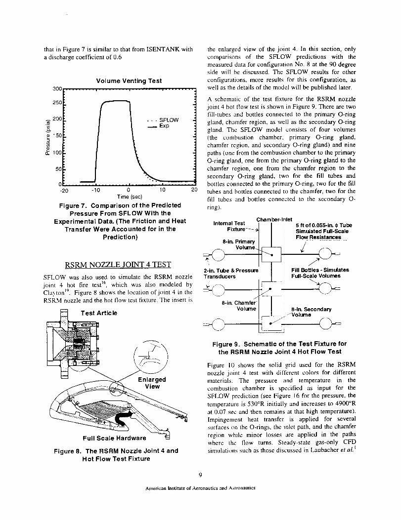
that in Figure 7 is similar to that from ISENTANK with
a discharge coefficient of 0.6
Volume Venting Test
300 ......... , ......... , ......... , .........
250
_2_
150
2100
5O
• --SFLOW_p
0 .... m .................. ; ..........-20 -10 0 10
Time (sec)
Figure 7. Comparison of the Predicted
Pressure From SFLOW With the
Experimental Data. (The Friction and Heat
Transfer Were Accounted for in the
Pred iction)
2o
RSRM NOZZLE JOINT 4 TEST
SFLOW was also used to simulate the RSRM nozzle
joint 4 hot fire test 16, which was also modeled by
Clavton =9. Figure 8 shows the location of joint 4 in the
RSRM nozzle and the hot flow test fixture. The insert is
Article
Figure 8. The RSRM Nozzle Joint 4 andHot Flow Test Fixture
the enlarged view of the joint 4. In this section, only
comparisons of the SFLOW predictions with the
measured data for configuration No. 8 at the 90 degree
side will be discussed. The SFLOW results for other
configurations, more results for this configuration, as
well as the details of the model will be published later.
A schematic of the test fixture for the RSRM nozzle
joint 4 hot flow test is shown in Figure 9. There are two
fill-tubes and bottles connected to the primary O-ring
gland, chamfer region, as well as the secondary O-ring
gland. The SFLOW model consists of four volumes
(the combustion chamber, primary O-ring gland,
chamfer region, and secondary O-ring gland) and nine
paths (one from the combustion chamber to the primary
O-ring gland, one from the primary O-ring gland to the
chamfer region, one from the chamfer region to the
secondary O-ring gland, two for the fill tubes and
bottles connected to the primary O-ring, two for the fill
tubes and bottles connected to the chamfer, two for the
fill tubes and bottles connected to the secondary O-
ring).
Internal Test_
Fixlure-_
8-in. Primary I
_ Volume._
2-in. Tube & PressureTransducers
___ /--_
8-in. Chamfer'Volume
Chamber-Inlet
15 ft of 0.055-in. ¢ TubeSimulated Full-ScaleFlow Resistances
-7
Fill Bottles - SimulatesFull-Scale Volumes
l 8-in. Secondary
---L_f i- zVolume
r
Figure 9. Schematic of the Test Fixture forthe RSRM Nozzle Joint 4 Hot Flow Test
Figure 10 shows the solid grid used for the RSRM
nozzle joint 4 test with different colors for different
materials. The pressure and temperature in the
combustion chamber is specified as input for the
SFLOW prediction (see Figure 16 for the pressure, the
temperature is 530°R initially and increases to 4900°R
at 0.07 sec and then remains at that high temperature).
Impingement heat transfer is applied for several
surfaces on the O-rings, the inlet path, and the chamfer
region while minor losses are applied in the paths
where the flow turns. Steady-state gas-only CFD
simulations such as those discussed in Laubacher et al.t
American Institute of Aeronautics and Astronautics

areusedto determinewhichsurfilcesshouldhavejetimpingementheattransfer.
Chamber
_ _ _ _r _ _'_ _
.... t.ea.
____ __ Path;-_'_r _ --_ Primary
_5> ,_-_,_ O-rin 9
i ::_ - . _ SY-;--_-"
_;:_ l_V_- ',_-_ Chamfer
.......... £; 2Secon.ar o-r,n0
'i I_ _--_Steel
Figure 10. The SFLOW Grid of the Solid forRSRM Joint 4 Hot Test Simulation
Isoc,mtours of the predicted temperatures of the solid at
4.(1 sec are sho_n in Figure I I. Initially the temperature
is at 530°R. At 4.0 sec, the solid cells near the
impinging surfaces as well as those near the flow path
from the chamber to the primary O-ring are hot while
the temperatures at the solid cells farther away are still
very low.
Solid Temperatures in the Whole
Computational Domain _,
i iii.
I,_c_lntt_ul-, _fl the prediclcd _lld temperatures at 1.0
,c_. 2!)_cc. 3.1/ scc. and 4 _ ,co are shown in Figure
!2. I:igurc 13, Figure 14. :rod Iqgure 15, respectively,
l:_l part ,q the domain illciuding the O-rings and
,:hantlcl-. ,\:, tinlc increLiscs, i/1()[c s_lid heats up while
t[lc tclltl+,crattlrcs oi the s_[id near the impingement
-,urfaccs decrease due t_ heat c_mduction. Since the
thermal ctmductivity is larger l_r steel than carbon
Solid Temperatures in Part of the
Computational Domain
Figure 12. Isocontours of SFLOW PredictedSolid at 1.0 sec
Solid Temperatures in Part of the
Computational Domain
Figure 11. Isocontours of SFLOW Predicted
Solid Temperatures at 4.0 sec
l_)
Figure13. IsocontoursofSFLOWPredicted
Solid Temperatures at 2.0 see
American Institute of .+\tJll!ll:ltltl,2_ +lild \,ttt+llLttltlC_,

Solid Temperatures in Part of the
Computational Domain
Figure14. IsocontoursofSFLOWPredicted
Solid Temperatures at 3.0 sec
Solid Temperatures in Part of the
Computational Domain
Figure15. IsocontoursofSFLOWPredicted
Solid Temperatures at 4.0 sec
l,r ;'IiL'm_lic IC('P). _t la[_'cr i_.'_1_,l_ q lhc _,Iccl is at a
h_ : ' r:mpcr:tturc thml CC[ >
r 1_:. i:1,_'u:c I- _::d l:_'ut: ['_ d:aw the
: :t,,l lhc _l:l _)\\ :,rc_I_,_,l _-x_i,_c_>ure with
' _'li,_,\c', Jh,lllllcF [J-'bq}, ,l13t! [ilL' scc_mdary 0-
: _:. ,,_. rc,lWctixcl,. :n I<MiRX! :l, /'it l,_mt 4. test..l_,_n m tl_c'sc li_u_cs _. _kc l_Ic",sLtrc of the
200
- 150
._,o
100
E.
50
Fill Bottle Pressure OffPrimary O-ring Groove: RSRM Joint 4
• . ........ ° . . . ° . .
a aExp
1 2 3
Time (sec)
Figure 16. Comparison of the PredictedGas Pressures With the Measured Data
200
.__ 150(/)
if_
50
Fill Bottle Pressure Off
Chamfer Region: RSRM Joint 4
,°
, o ......... . . ° o , o °
hamber
oT g ow....... _l ......... , ......... i .....
1 2 3
Time (sec)
Figure 17, Comparison of the PredictedGas Pressures With the Measured Data
4
11
Fill Bottle Pressure Off SecondaryO-ring Groove: RSRM Joint 4
......... i ......... , ......... , .........
200' ""
°° ......... o ° • . . . ° o i
Chamber
SFLOW
Exp
5O
........ | ....
0 1 2 3
Time (sec)
Figure 18. Comparison of the Predicted GasPressures With the Measured Data
__ 150
100
kmctlL'4n Institute of Aeronautics and Astronautics

combustion chamber, which is an input to the SFLOW
code. The pressures at all the fill bottles are very
similar and the predicted values agree very well withthe measured data.
The predicted temperatures of the fill bottles in the
RSRM nozzle joint 4 test are compared with themeasured data in Figure 19. The agreement is good
considering that the chamber temperature is about
5,000°R while that in the fill bottles is less than 600°R.
Fill Bottle Temperatures: RSRM Joint 4
56O
540
I •••ch.mfe,Bot,e. .1
_ Secondary Bottle, SFLOW V
I.- Itt II Primary Bottle, Exp520O O Chamfer Bottle, Exp
X X Secondary Bottle, Exp
500 ....................................0 1 2 3 4
Time (sec)
Figure 1 9. Comparison of the Predicted Gas
Temperatures With the Measured Data
Figure 20 and Figure 21 show the predicted solid
temperatures at two locations, one near the primary O-
ring (TI4 in Figure 22) and the other just before thesecondary O-ring (TI5 in Figure 22), together with themeasured data at the same locations. As discussed by
Temperature Versus Time: RSRM Joint 4
2,5001 ......... _ _ ........ _ .........! _ _ SFLOW
zoool /
_- 1,000t: _._ , , _'_,m_,500[ E
0 1 2 3 4Time (sec)
Figure 20. Comparison of the Predicted
Temperature of the Solid Near the Primary O-
ring (T14 in Figure 22) With the Measured Data
Temperature Versus Time:RSRM Joint 4
1,000
900
800
_" 700I-
600
50O
-- SFLOW
_ Exp_
J I I
0 1 2 3 4
Time (sec)
Figure 21. Comparison of the Predicted
Temperature of the Solid Near the
Secondary O-ring (T15 in Figure 22) Withthe Measured Data
_-fl, fl P1,TIA
P_T_
_,X / ,"X t
_://,/,,¥ -k ~ _-o.t_"'/;'i+'i[ \ ,tom.
\... qr.... I" ,,_,t,_® , IL_i.
Figure 22. The Location of the Thermocouplesin the RSRM Nozzle Joint 4 Test
Clayton _'_, the measured temperatures are not veryaccurate due to the large gradients, tiny gaps and brief
time scales. On the other hand, better agreement might
be obtained by using a full three-dimensional solid grid.
12
American Institute of Aeronautics and Astronautics

The predicted erosion of the secondary O-ring is shownin Figure 23. The predicted total erosion after 2 sec is
about 0.00813 in, which is very close to the measuredvalue of 0.008 in. This agreement is excellent
considering analytical modeling complexity andassumptions required, as well as the variability inmeasured data, measurement error due to very small
dimensions and short time frame.
0.010 t- ........ , ......... , .......... . ........
Fo.oo8F
[0.006o.oo,
_ o.oo2 I
0 000 ......0 1 2 3
Time (sec)
Figure 23. Secondary O-ringErosion Predicted by
SFLOW in RSRM Nozzle Joint 4 Test
discussed above, most CFD applications in theAs
RSRM joints do not include the solid region in the
computational domain and the solid wall is assumed tobe either adiabatic or isothermal. Figure 24 and Figure
25 compare the SFLOW predictions of the pressures
and gas temperatures in the fill bottles with and withoutheat transfer between the gas and solid. It indicates that,without heat transfer, the fill time is reduced by a/'actor
of about three and the gas temperature increases to
more than 1,400°R from around 580°R with heat
transfer. For these conditions, heat transfer to the solid
wall is a significant driver for the problem.
200,
150
$ lOO.
50t
2,000
1,500
Fill Bottle Pressures: RSRM Joint 4
ill
0 1
- Primary Bottle, w/o HT
-- Chamfer Bottle, w/o HT
-- Secondary Bottle,w/o HT_ Primary Bottle, With PIT
[] _ Chamfer Bottle, With HT
× _ Secondary Bottle, With HTI
2 3
Time (sec)
Figure 24. Comparison of theSFLOW Predicted Gas Pressure With and
Without Heat Transfer
:ill Bottle Temperatures: RSRM Joint 4
.......i.....j//'
, . /JI
f j" ',/ / _ .
1,000 ' ,_
Primary Bottle, w/o HT
Chamfer Bottle, _to HT
Secondary Bottle, w/o HT
Primary Bottle, With HT
-_ Chamfer Bottle, W'rth HT
× Secondary Bottle, With HT
500 :_ai=aalBii_ela=i,a,l_.,l. =t=t
0 1 2 3
Time (sec)
Figure 25. Comparison of theSFLOW Predicted Gas Temperature With
and Without Heat Transfer
13
American Institute of Aeronautics and Astronautics

SUMMARY AND CONCLUSIONS
A new thermal-flow simulation code, called SFLOW.
has been developed to model the gas dynamics, heat
transfer, as well as O-ring and flow path erosion insidethe space shuttle solid rocket motor joints by
combining SINDA/G ®, a commercial thermal analyzer.
and SHARP*, a general-purpose CFD code developed
at Thiokol Propulsion. SHARP* was modified so thatfriction, heat transfer, mass addition, as well as minorlosses in one-dimensional flow can be taken into
account. The pressure, temperature and velocity of thecombustion gas in the leak paths are calculated in
SHARP _ by solving the time-dependent Navier-Stokes
equations while the heat conduction in the solid is
modeled by SINDA/G ®. The two codes are coupled by
the heat flux at the solid-gas interface.
A few test cases are presented and the results from
SFLOW agree very well with the exact solutions orexperimental data. These cases include Fanno flow
where friction is important, Rayleigh flow where heat
transfer between gas and solid is important, flow withmass addition due to the erosion of the solid wall, a
transient volume venting process, as well as sometransient one-dimensional flows with analytical
solutions. In addition, SFLOW is applied to model the
RSRM nozzle joint 4 subscale hot-flow tests and the
predicted pressures, temperatures (both gas and solid),and O-ring erosions agree well with the experimentaldata. It was also found that the heat transfer between
gas and solid has a major effect on the pressures and
temperatures of the fill bottles in the RSRM nozzle
joint 4 configuration No. 8 test.
REFERENCE
I. Laubacher, B.A., Eaton, A.M., Pate, R.A., Wang.
Q., Mathias, E.C. and Shipley, J.L. 1999 "Cold-flow simulation and CFD modeling of the space
shuttle solid rocket motor nozzle joints," AIAA
Paper 99-2793.
2. Eaton A. and Mathias, E. 2000 "Simulating heat
transfer to a solid rocket motor nozzle-case-joint
thermal barrier," AIAA Paper 2000-3807.
3. O'Malley, M.J. 1988 "A model lor predicting
RSRM joint volume pressurization, temperaturetransients, and ablation," AIAA Paper 88-3332.
4. O'Malley, M.J. 1987a "ORING2: volume filling
and O-ring erosion prediction code with improvedmodel descriptions and validation, Part I:
Improved O-ring Erosion Prediction Code,"
Thiokol Corporation TWR- 17030
5. O'Malley, M.J. 1987b "ORING2: volume filling
and O-ring erosion prediction code with improved
14
model descriptions and validation, Part II:
Improved volume filling model and codevalidation," Thiokol Corporation TWR- 1703 I
6. O'Malley, M.J. 1990 "ORING2: volume filling and
O-ring erosion prediction code with improved
model descriptions and validation, Part III: User'sguide," Thiokol Corporation TWR-50398
7. Clayton, J.L. 1995 "Joint pressurization routine(JPR) theoretical development and users manual,"NASA-MSFC Internal Memorandum ED66 (95-
01).
8. Network Analysis Inc. 1996 SINDA/G ® User's
Guide, Tempe, AZ.
9. Golafshani, M. and Loh, H.T. 1989 "Computation
of two-phase viscous flow in solid rocket motors
using a flux-split Eulerian-Lagrangian technique,"
AIAA Paper 89-2785.
10. Loh, H.T. and Golafshani, M. 1990 "Computation
of viscous chemically reacting flows in hybridrocket motors using an upwind LU-SSOR
scheme," AIAA paper 90-1570.
11. Loh, H.T., Smith-Kent, R., Perkins, F and
Chwalowski, P. 1996 "Evaluation of aft skirt
length effects on rocket motor base heat usingcomputational fluid dynamics," AIAA paper 96-2645.
12. Wang, Q. 1999a "Theory Manual for SHARP*: a
general CFD solver," Thiokol Corporation TR-11580
13. Wang, Q. 1999b "Programer's guide for SHARP*:
a general CFD solver," Thiokol Corporation TR-11581
14. Wang, Q. 1999c "User's guide for SHARP*: a
general CFD solver," Thiokol Corporation TR-11582
15. Cai, R. 1998 "Some explicit analytical solutions of
unsteady compressible flow," Journal of Fluid
Eng., Vol. 120, pp. 760-764.
16. Prince, A. 1999 "Final report for ETP-1385:
Tortuous path thermal analysis test bed," Thiokol
Corporation TWR-66623.
17. Idelchik, I.E. 1986 Handbook of HydraulicResistapce, 2"j Edition, Hemisphere Publishing
Corp.
18. Wang, Q. 1998 "ISENTANK code," Thiokol
Corporation MEMO 32B2-FY98-M029.
19. Clayton, J.L. 1999 "Reusable solid rocket motor
nozzle joint-4 test correlated gas dynamics-thermal
analysis," AIAA Paper 99-279 I.
American Institute of Aeronautics and Astronautics