Daniella Lopez (41834598)Dr. Dimas/ MAE1521/29/2015

Homework#3 [ch.7]: Thermal analysis of a pipe connector and a heater

PIPE CONNECTOR:

In this problem a pipe connector made of Brass has four openings with different thermal loads on each face of the opening. The objective is to apply the thermal loads to the corresponding sides and conduct a steady state thermal analysis that calculates a temperature distribution plot, heat flux plot, and apply a static analysis with the thermal loads to calculate thermal stress.

Thermal Loads: (top) 80°C, (right) 400°C, (bottom) 250°C, (left) 100°C

Thermal boundary conditions are applied, which are provided by SolidWorks. The mesh created is very fine as we can see from the mesh details and the figure above. This allows fairly accurate calculations.

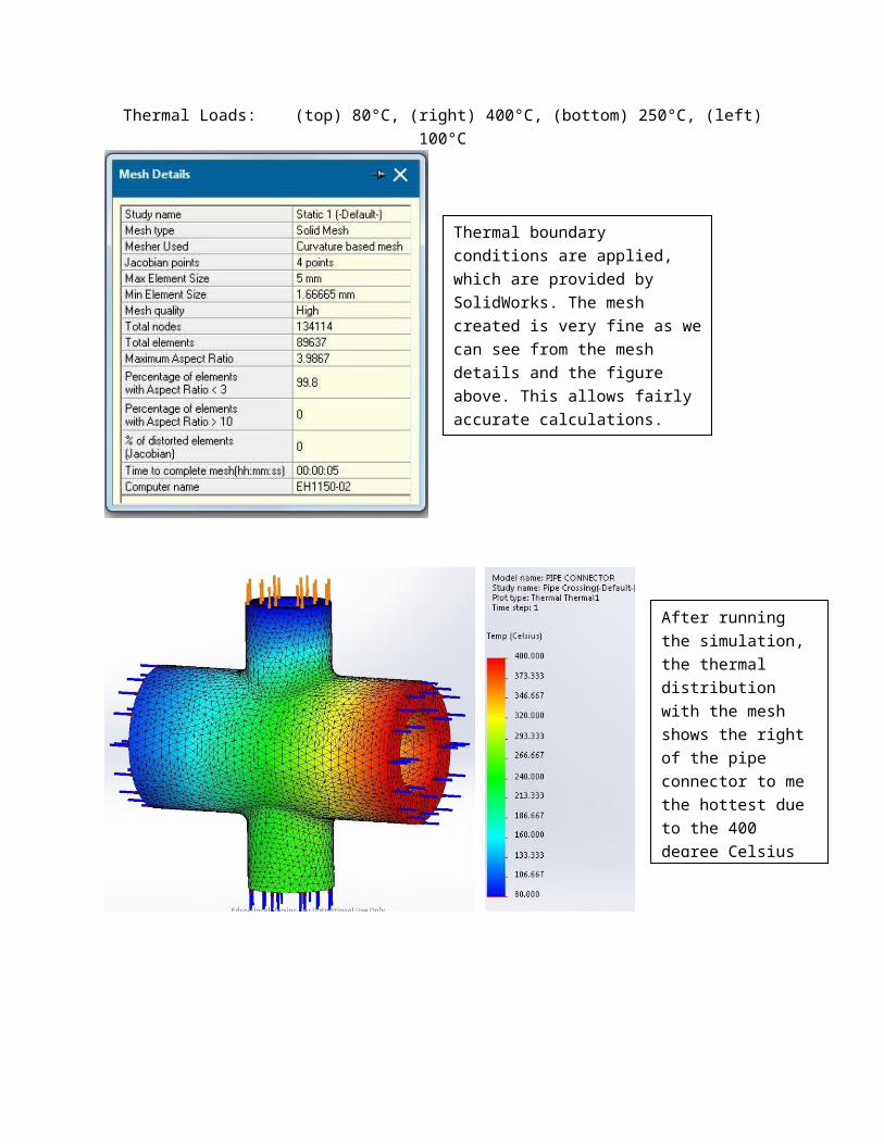
After running the simulation, the thermal distribution with the mesh shows the right of the pipe connector to me the hottest due to the 400 degree Celsius thermal load. The max temp is 400C while the minimum is 80C which is at the top of the pipe.

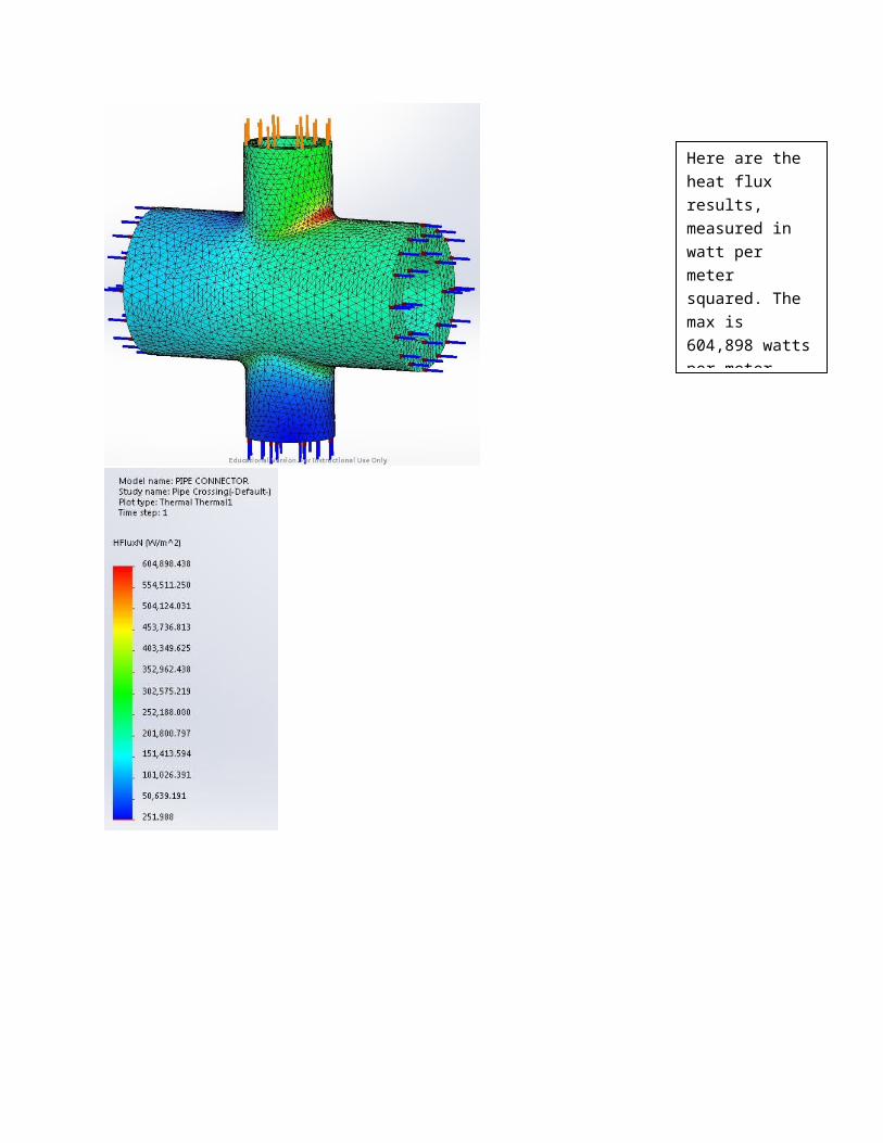
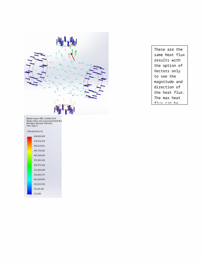
Here are the heat flux results, measured in watt per meter squared. The max is 604,898 watts per meter squared at the fillet of the top opening of the pipe connector.

These are the same Heat flux results with the option of Vectors only to see the magnitude and direction of the heat flux. The max heat flux can be seen with more precision.

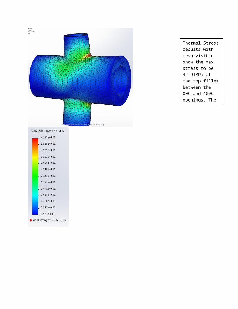
Thermal Stress results with mesh visible show the max stress to be 42.91MPa at the top fillet between the 80C and 400C openings. The yield strength is 239MPa.

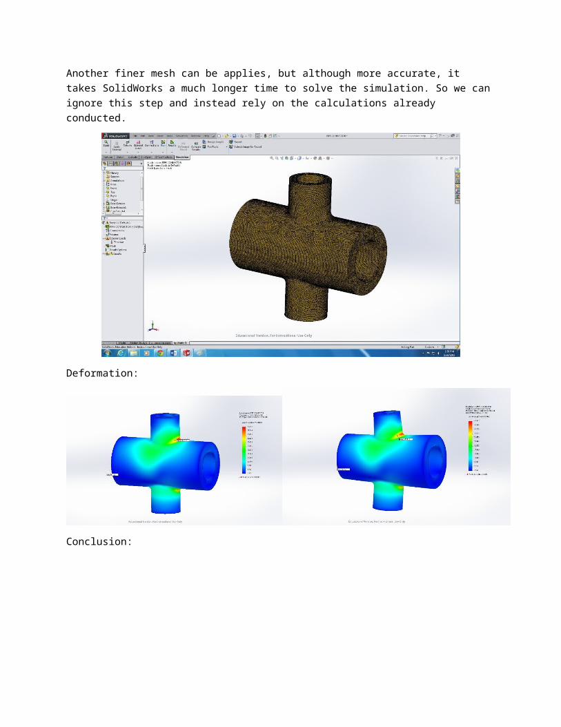
Another finer mesh can be applies, but although more accurate, it takes SolidWorks a much longer time to solve the simulation. So we can ignore this step and instead rely on the calculations already conducted.

Deformation:

Conclusion:

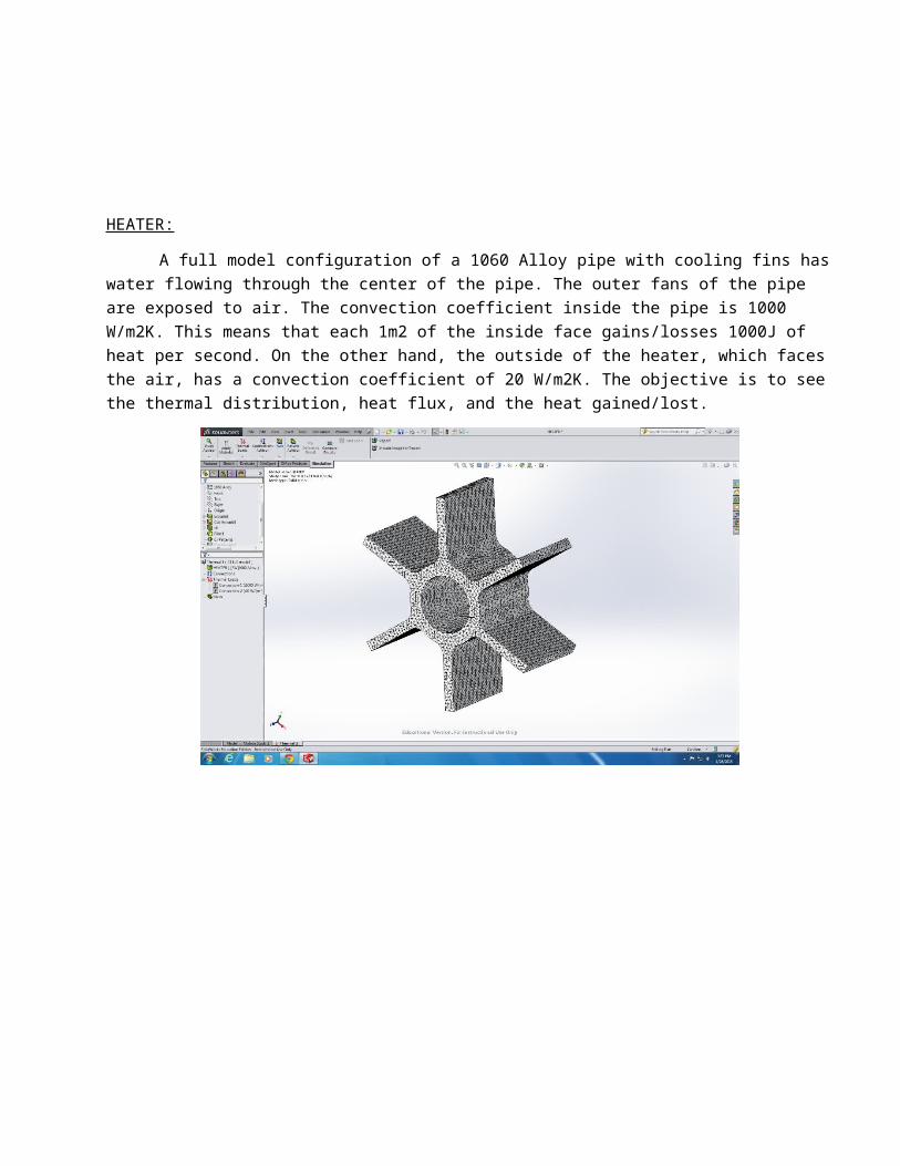
HEATER:

A full model configuration of a 1060 Alloy pipe with cooling fins has water flowing through the center of the pipe. The outer fans of the pipe are exposed to air. The convection coefficient inside the pipe is 1000 W/m2K. This means that each 1m2 of the inside face gains/losses 1000J of heat per second. On the other hand, the outside of the heater, which faces the air, has a convection coefficient of 20 W/m2K. The objective is to see the thermal distribution, heat flux, and the heat gained/lost.

Here is the thermal distribution of the heater. The max temperature is 92.75 C at the center of the pipe fan where it is closest to the high temperature water. The fan ends are the coolest at 90.48 C, but is very hot compared to ambient air at 27 C.

Here is the heat flux in the heater. The max heat flux is 17,721.5 W/m^2 located at the fillets of the fan blades. The lowest heat flux located at the ends of the blades is 2.161 W/m^2.

Conclusion:

When the center of the heater is selected (left) the summary shows the power in to be 39.317 W. When the entire outside of the heater fan is selected (right), the power out is 39.317 W. Power in equals the power out.