Thermal Analysis - METTLER TOLEDO Balances & … Notes Petroleum Products 5 METTLER TOLEDO Thermal Analysis Preface Thermal analysis is one of the oldest analysis techniques. Throughout

Advanced Thermal AnalysisApplied to Petroleum Products

Ther

mal

Ana

lysi

s

ApplicationNotes

Application Notes Petroleum Products METTLER TOLEDO Thermal Analysis

3

Application NotesThermal Analysis

Advanced Thermal Analysis Applied to Petroleum Products

This application handbook presents selected application examples. The experiments were conducted with the utmost care using the instruments speci-fied in the description of each application. The results were evaluated according to the current state of our knowledge.

This does not however absolve you from personally testing the suitability of the examples for your own methods, instruments and purposes. Since the transfer and use of an application is beyond our control, we cannot of course accept any responsibility.

When chemicals, solvents and gases are used, general safety rules and the instructions given by the manufacturer or supplier must be observed.

® TM All names of commercial products can be registered trademarks, even if they are not denoted as such

4 Application Notes Petroleum Products METTLER TOLEDO Thermal Analysis

5Application Notes Petroleum Products METTLER TOLEDO Thermal Analysis

Preface

Thermal analysis is one of the oldest analysis techniques. Throughout history, people have used simple heat tests to determine whether materials were genuine or fake.

The year 1887 is looked upon as the dawn of present-day thermal analysis. It was then that Henry Le Chatelier, the famous French scientist, carried out his first thermometric measurements on clays. Just a few years later in 1899, the British scientist William Roberts-Austen performed the first differential temperature measurements and so initiated the development of DTA. Commercial instruments however, did notappear until the early 1960s. Since then, thermal analysis has undergone fifty years of intense devel-opment. Thermal analysis is the ideal technique for determining material properties and transitions and for characterizing materials.

This compilation of application notes focuses on applications of thermal analysis techniques in the field of petroleum products. The chapters were previously published in different issues of METTLER TOLEDO's UserCom, a bi-annual technical customer mag-azine, and Collected Applications Handbooks.

From crude oil to gasoline, diesel, liquid gas, lubricants, polymers, plastics and many other end products, petrochemicals are ever present in our lives. The number of standards and regulations for analysis further reflects the importance and variety of petro-chemical raw materials and products. In today’s competitive environment, demands are acute when it comes to meeting quality and regulatory requirements, improving yield, and reducing downtime, corrosion and waste. To stay in control, you need instru-mentation that provides more than just a measurement. In addition, you also need a supplier partner who delivers solutions and provides advice, application support and technical assistance.

We hope that the introductory chapters and applications described here will be of interest and make you aware of the great poten-tial of thermal analysis methods in the petroleum products field.


Cont

ents

Contents1 Introduction to thermal analysis 8

1.1 Differential scanning calorimetry (DSC) 8 1.1.1 Conventional DSC 8 1.1.2 Temperature-modulated DSC 9

1.1.2.1 ADSC 9 1.1.1.2 IsoStep® 10 1.1.2.3 TOPEM® 11

1.2 Thermogravimetric analysis (TGA) 121.3 Thermomechanical analysis (TMA) 131.4 Dynamic mechanical analysis (DMA) 131.5 Simultaneous measurements with TGA 15

1.5.1 Differential thermal analysis (DTA, SDTA®) 15 1.5.2 Evolved gas analysis (EGA) 15

1.5.2.1 TGA-MS 15 1.5.2.2 TGA-FTIR 16

2 Characterization of petroleum products with DSC 172.1 Introduction 172.2 Characterization of petroleum products with DSC 182.3 Evaluation of DSC curves of petroleum products 182.4 Conclusions 20

3 Oxidative stability of petroleum oil fractions 223.1 Introduction 223.2 Samples and measurement parameters 223.3 Interpretation 223.4 Evaluation 223.5 Conclusions 23

4 Determination of the Noack evaporation loss of lubricants by TGA 24

4.1 Abstract 244.2 Introduction 244.3 The Noack evaporation loss test according to

ASTM D6375 244.4 Performing a Noack test 254.5 Conclusions 26

5 Rapid thermogravimetric analysis of coal 275.1 Introduction 275.2 Speeding up the TGA procedure 275.3 Experimental details 285.4 Results 295.5 Conclusions 30


6 Determination of oxidation stability by pressure-dependent OIT measurements 31

6.1 Introduction 316.2 Experimental details 326.3 Pressure dependence of OIT 326.4 Interpretation of the results 346.5 Assessment of experimental results 356.6 Conclusions 36

7. Standards for petrochemicals with respect to thermal analysis 37

7.1 More analytical instruments from METTLER TOLEDO 37

8. More Information 38


Intro

duct

ion

to th

erm

al a

naly

sis

Thermal analysis is the name given to a group of techniques used to measure the physical and chemical proper-ties of materials as a function of temperature. In all these methods, the sample is subjected to a heating, cooling or isothermal temperature program.The measurements can be performed in different atmospheres. Usually either an inert atmosphere (nitrogen, argon, helium) or an oxidative atmosphere (air, oxygen) is used. In some cases, the gases are switched from one atmosphere to another during the measurement. Another parameter sometimes selectively varied is the gas pressure.DSC can also be used in combination with instruments that allow the sample to be simultaneously observed (DSC microscopy) or exposed to light of different wavelengths (photocalorimetry).

1.1 Differential scanning calorimetry (DSC)

In DSC, the heat flow to and from the sample is measured. DSC can be used to investigate thermal events such as physi cal transitions (the glass transition, crystallization, melting, and the vaporization of volatile compounds) and chemical reactions. The information obtained characterizes the sample with regard to its thermal behavior and composition. In addition, properties such as the heat capacity, glass transition temperature, melting tem-perature, heat and extent of reaction can also be determined.

1.1.1 Conventional DSC

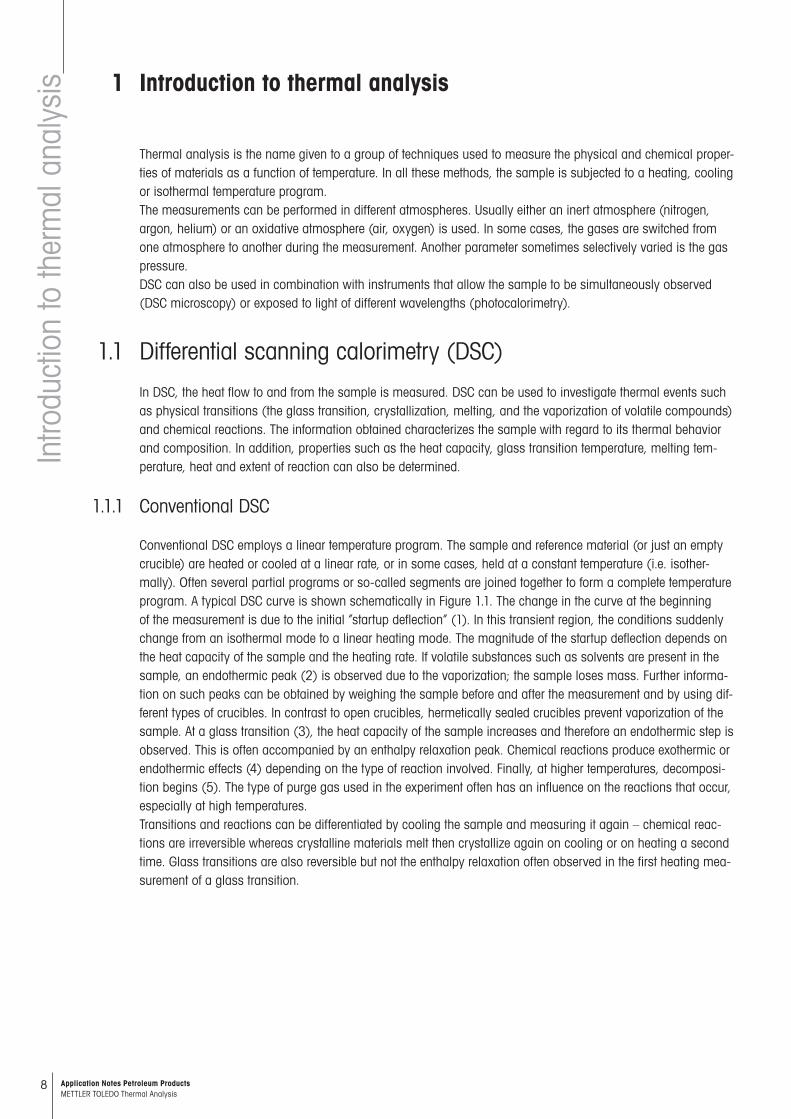
Conventional DSC employs a linear temperature program. The sample and reference material (or just an empty cruci ble) are heated or cooled at a linear rate, or in some cases, held at a constant temperature (i.e. isother-mally). Often several partial programs or so-called segments are joined together to form a complete temperature program. A typical DSC curve is shown schematically in Figure 1.1. The change in the curve at the beginning of the measurement is due to the initial “startup deflection” (1). In this transient region, the conditions suddenly change from an isothermal mode to a linear heating mode. The magnitude of the startup deflection depends on the heat capacity of the sample and the heating rate. If volatile substances such as solvents are present in the sample, an endothermic peak (2) is observed due to the vaporization; the sample loses mass. Further informa-tion on such peaks can be obtained by weighing the sample before and after the measurement and by using dif-ferent types of crucibles. In contrast to open crucibles, hermetically sealed crucibles prevent vaporization of the sample. At a glass transition (3), the heat capacity of the sample increases and therefore an endothermic step is observed. This is often accompanied by an enthalpy relaxation peak. Chemical reactions produce exothermic or endothermic effects (4) depending on the type of reaction involved. Finally, at higher temperatures, decomposi-tion begins (5). The type of purge gas used in the experiment often has an influence on the reactions that occur, especially at high temperatures.Transitions and reactions can be differentiated by cooling the sample and measuring it again – chemical reac-tions are irreversible whereas crystalline materials melt then crystallize again on cooling or on heating a second time. Glass tran sitions are also reversible but not the enthalpy relaxation often observed in the first heating mea-surement of a glass transition.

1 Introduction to thermal analysis


Figure 1.1. Schematic DSC curve: 1 initial startup deflection; 2 evaporation of moisture; 3 glass transition with relaxation peak; 4 reaction (e.g. curing); 5 beginning of decomposition.

1.1.2 Temperature-modulated DSC

1.1.2.1 ADSC

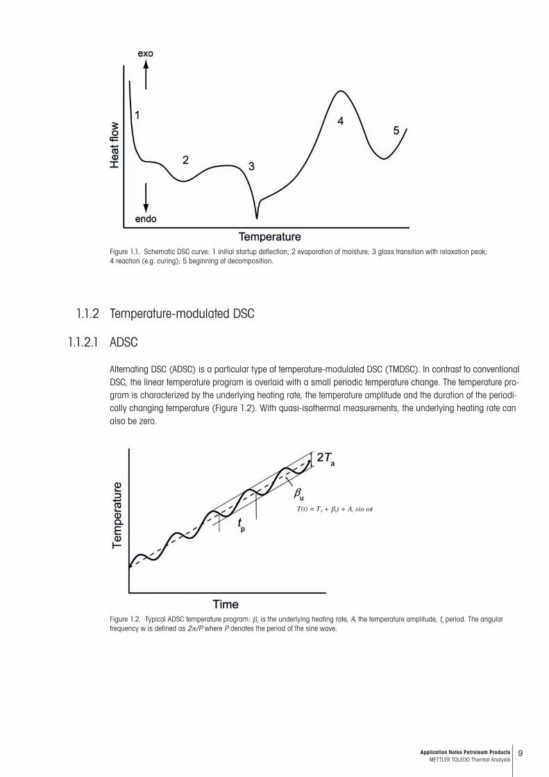
Alternating DSC (ADSC) is a particular type of temperature-modulated DSC (TMDSC). In contrast to conventional DSC, the linear temperature program is overlaid with a small periodic temperature change. The temperature pro-gram is char acterized by the underlying heating rate, the temperature amplitude and the duration of the periodi-cally changing tem perature (Figure 1.2). With quasi-isothermal measurements, the underlying heating rate can also be zero.

Figure 1.2. Typical ADSC temperature program: bu is the underlying heating rate, AT the temperature amplitude, tp period. The angular frequency w is defined as 2p/P where P denotes the period of the sine wave.

T(t) = T0 + but + At sin wt


Intro

duct

ion

to th

erm

al a

naly

sis

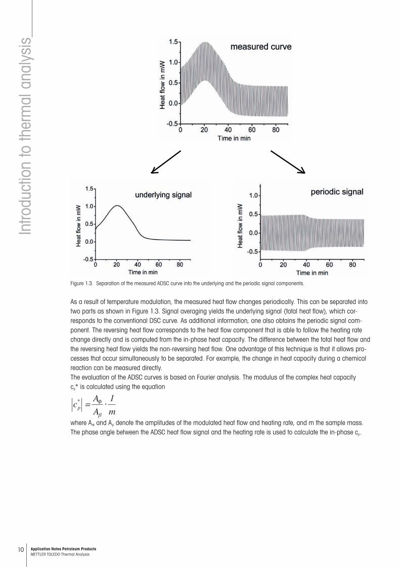
Figure 1.3. Separation of the measured ADSC curve into the underlying and the periodic signal components.

As a result of temperature modulation, the measured heat flow changes periodically. This can be separated into two parts as shown in Figure 1.3. Signal averaging yields the underlying signal (total heat flow), which cor-responds to the con ventional DSC curve. As additional information, one also obtains the periodic signal com-ponent. The reversing heat flow corresponds to the heat flow component that is able to follow the heating rate change directly and is computed from the in-phase heat capacity. The difference between the total heat flow and the reversing heat flow yields the non-reversing heat flow. One advantage of this technique is that it allows pro-cesses that occur simultaneously to be separated. For exam ple, the change in heat capacity during a chemical reaction can be measured directly.The evaluation of the ADSC curves is based on Fourier analysis. The modulus of the complex heat capacity cp* is calcu lated using the equation

mAAcp

1* =

where AF and Ab denote the amplitudes of the modulated heat flow and heating rate, and m the sample mass. The phase angle between the ADSC heat flow signal and the heating rate is used to calculate the in-phase cp.


1.1.1.2 IsoStep®

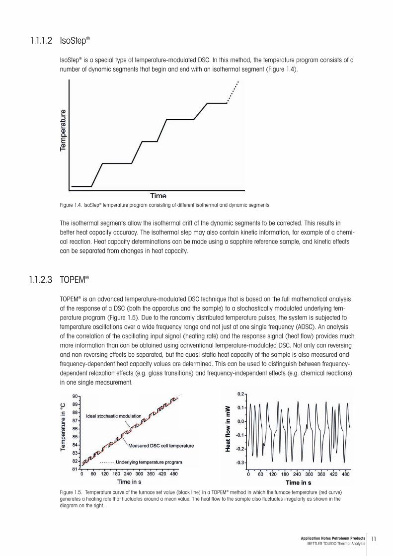
IsoStep® is a special type of temperature-modulated DSC. In this method, the temperature program consists of a number of dynamic segments that begin and end with an isothermal segment (Figure 1.4).

Figure 1.4. IsoStep® temperature program consisting of different isothermal and dynamic segments.

The isothermal segments allow the isothermal drift of the dynamic segments to be corrected. This results in better heat capacity accuracy. The isothermal step may also contain kinetic information, for example of a chemi-cal reaction. Heat capacity determinations can be made using a sapphire reference sample, and kinetic effects can be separated from changes in heat capacity.

1.1.2.3 TOPEM®

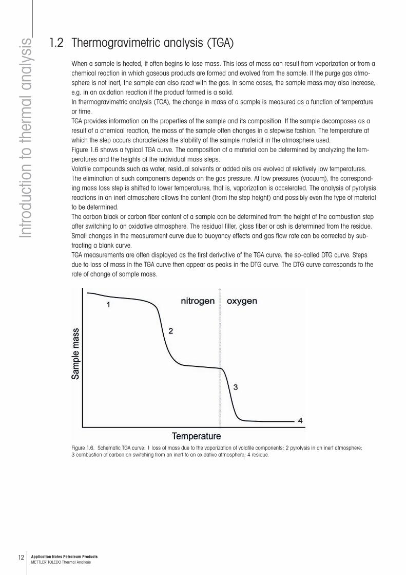
TOPEM® is an advanced temperature-modulated DSC technique that is based on the full mathematical analysis of the response of a DSC (both the apparatus and the sample) to a stochastically modulated underlying tem-perature program (Figure 1.5). Due to the randomly distributed temperature pulses, the system is subjected to temperature oscillations over a wide frequency range and not just at one single frequency (ADSC). An analysis of the correlation of the oscillating input signal (heating rate) and the response signal (heat flow) provides much more information than can be obtained using conventional temperature-modulated DSC. Not only can reversing and non-reversing effects be separated, but the quasi-static heat capacity of the sample is also measured and frequency-dependent heat capacity values are determined. This can be used to distinguish between frequency-dependent relaxation effects (e.g. glass transitions) and frequency-in de pendent effects (e.g. chemical reactions) in one single measurement.

Figure 1.5. Temperature curve of the furnace set value (black line) in a TOPEM® method in which the furnace temperature (red curve) generates a heating rate that fluctuates around a mean value. The heat flow to the sample also fluctuates irregularly as shown in the diagram on the right.


Intro

duct

ion

to th

erm

al a

naly

sis 1.2 Thermogravimetric analysis (TGA)

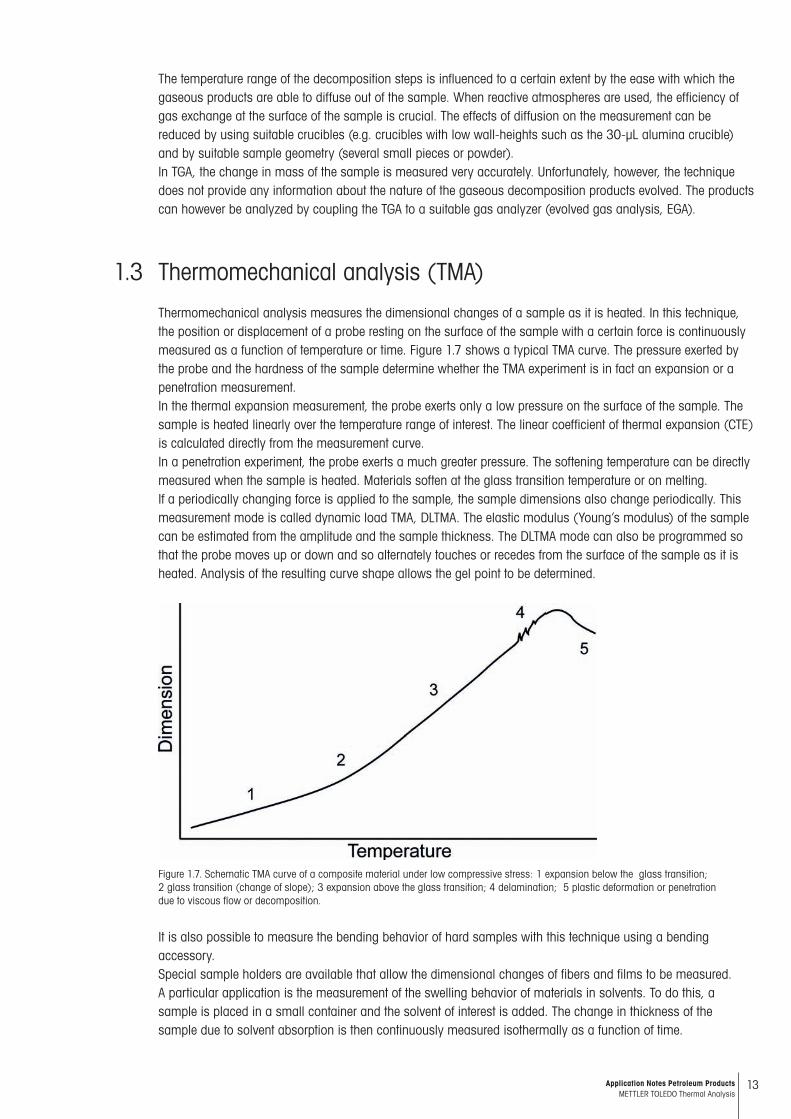
When a sample is heated, it often begins to lose mass. This loss of mass can result from vaporization or from a chemical reaction in which gaseous products are formed and evolved from the sample. If the purge gas atmo-sphere is not inert, the sample can also react with the gas. In some cases, the sample mass may also increase, e.g. in an oxidation reaction if the product formed is a solid.In thermogravimetric analysis (TGA), the change in mass of a sample is measured as a function of temperature or time.TGA provides information on the properties of the sample and its composition. If the sample decomposes as a result of a chemical reaction, the mass of the sample often changes in a stepwise fashion. The temperature at which the step occurs characterizes the stability of the sample material in the atmosphere used.Figure 1.6 shows a typical TGA curve. The composition of a material can be determined by analyzing the tem-peratures and the heights of the individual mass steps.Volatile compounds such as water, residual solvents or added oils are evolved at relatively low temperatures. The elimi nation of such components depends on the gas pressure. At low pressures (vacuum), the correspond-ing mass loss step is shifted to lower temperatures, that is, vaporization is accelerated. The analysis of pyrolysis reactions in an inert atmos phere allows the content (from the step height) and possibly even the type of material to be determined.The carbon black or carbon fiber content of a sample can be determined from the height of the combustion step after switching to an oxidative atmosphere. The residual filler, glass fiber or ash is determined from the residue. Small changes in the measurement curve due to buoyancy effects and gas flow rate can be corrected by sub-tracting a blank curve.TGA measurements are often displayed as the first derivative of the TGA curve, the so-called DTG curve. Steps due to loss of mass in the TGA curve then appear as peaks in the DTG curve. The DTG curve corresponds to the rate of change of sample mass.

Figure 1.6. Schematic TGA curve: 1 loss of mass due to the vaporization of volatile components; 2 pyrolysis in an inert atmosphere; 3 combustion of carbon on switching from an inert to an oxidative atmosphere; 4 residue.


The temperature range of the decomposition steps is influenced to a certain extent by the ease with which the gaseous products are able to diffuse out of the sample. When reactive atmospheres are used, the efficiency of gas exchange at the surface of the sample is crucial. The effects of diffusion on the measurement can be reduced by using suitable crucibles (e.g. crucibles with low wall-heights such as the 30-µL alumina crucible) and by suitable sample geometry (several small pieces or powder).In TGA, the change in mass of the sample is measured very accurately. Unfortunately, however, the technique does not provide any information about the nature of the gaseous decomposition products evolved. The products can however be analyzed by coupling the TGA to a suitable gas analyzer (evolved gas analysis, EGA).

1.3 Thermomechanical analysis (TMA)

Thermomechanical analysis measures the dimensional changes of a sample as it is heated. In this technique, the posi tion or displacement of a probe resting on the surface of the sample with a certain force is continuously measured as a function of temperature or time. Figure 1.7 shows a typical TMA curve. The pressure exerted by the probe and the hard ness of the sample determine whether the TMA experiment is in fact an expansion or a penetration measurement.In the thermal expansion measurement, the probe exerts only a low pressure on the surface of the sample. The sample is heated linearly over the temperature range of interest. The linear coefficient of thermal expansion (CTE) is calculated directly from the measurement curve.In a penetration experiment, the probe exerts a much greater pressure. The softening temperature can be directly meas ured when the sample is heated. Materials soften at the glass transition temperature or on melting.If a periodically changing force is applied to the sample, the sample dimensions also change periodically. This meas urement mode is called dynamic load TMA, DLTMA. The elastic modulus (Young’s modulus) of the sample can be esti mated from the amplitude and the sample thickness. The DLTMA mode can also be programmed so that the probe moves up or down and so alternately touches or recedes from the surface of the sample as it is heated. Analysis of the resulting curve shape allows the gel point to be determined.

Figure 1.7. Schematic TMA curve of a composite material under low compressive stress: 1 expansion below the glass transition; 2 glass transition (change of slope); 3 expansion above the glass transition; 4 delamination; 5 plastic deformation or penetration due to viscous flow or decomposition.

It is also possible to measure the bending behavior of hard samples with this technique using a bending accessory.Special sample holders are available that allow the dimensional changes of fibers and films to be measured. A particular application is the measurement of the swelling behavior of materials in solvents. To do this, a sample is placed in a small container and the solvent of interest is added. The change in thickness of the sample due to solvent absorption is then continuously measured isothermally as a function of time.


Intro

duct

ion

to th

erm

al a

naly

sis 1.4 Dynamic mechanical analysis (DMA)

In dynamic mechanical analysis, a mechanical modulus is determined as a function of temperature, frequency and amplitude.A periodically changing force (usually sinusoidal) applied to the sample creates a periodic stress in the sample. The sample reacts to this stress and the instrument measures the corresponding deformation behavior. The me-chanical modulus, M, is determined from the stress and deformation. Depending on the type of stress applied, ei-ther the shear modulus, G (with shear stress) or the Young’s modulus, E (with stretching or bending) is measured.The sample does not always immediately react to the periodically changing stress – a certain time delay occurs that depends on the viscoelastic properties of the sample. This is the cause of the phase shift between the applied stress and the deformation. To take this phase shift into account, the dynamically measured modulus is described by a real part M’ and an imaginary part M’’. The real part (storage modulus) describes the response of the sample in phase with the peri odic stress. It is a measure of the (reversible) elasticity of the sample. The imaginary part (loss modulus) describes the component of the response that is phase-shifted by 90°. This is a measure of mechanical energy converted to heat (and therefore irreversibly lost). The tangent of the phase shift, tan d, is also known as the loss factor and is a measure of the damping behavior of the material. The modulus and tan d depend on the temperature and the measuring frequency. At room temperature, rubbery materials show typical storage modulus values between 0.1 MPa and 10 MPa.

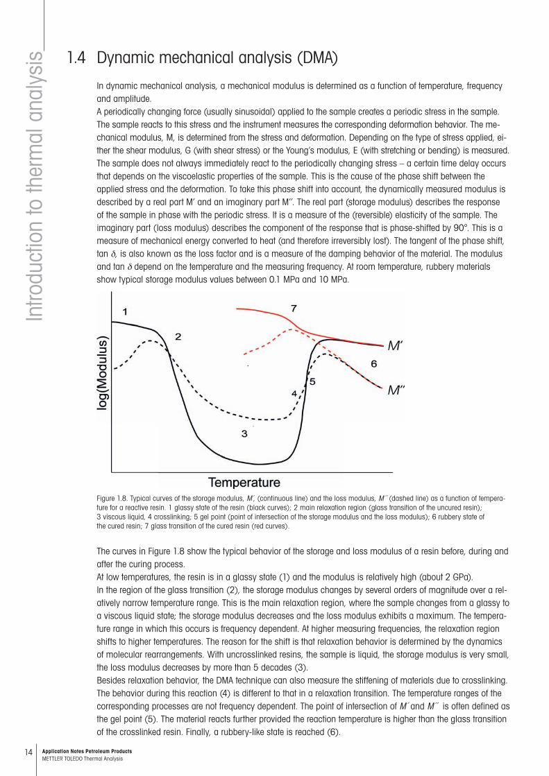
Figure 1.8. Typical curves of the storage modulus, M ,́ (continuous line) and the loss modulus, M´´ (dashed line) as a function of tempera-ture for a reactive resin. 1 glassy state of the resin (black curves); 2 main relaxation region (glass transition of the uncured resin); 3 viscous liquid, 4 crosslinking; 5 gel point (point of intersection of the storage modulus and the loss modulus); 6 rubbery state of the cured resin; 7 glass transition of the cured resin (red curves).

The curves in Figure 1.8 show the typical behavior of the storage and loss modulus of a resin before, during and after the curing process.At low temperatures, the resin is in a glassy state (1) and the modulus is relatively high (about 2 GPa).In the region of the glass transition (2), the storage modulus changes by several orders of magnitude over a rel-atively narrow temperature range. This is the main relaxation region, where the sample changes from a glassy to a viscous liquid state; the storage modulus decreases and the loss modulus exhibits a maximum. The tempera-ture range in which this occurs is frequency dependent. At higher measuring frequencies, the relaxation region shifts to higher temperatures. The reason for the shift is that relaxation behavior is determined by the dynamics of molecular rearrangements. With uncrosslinked resins, the sample is liquid, the storage modulus is very small, the loss modulus decreases by more than 5 decades (3).Besides relaxation behavior, the DMA technique can also measure the stiffening of materials due to crosslinking. The behavior during this reaction (4) is different to that in a relaxation transition. The temperature ranges of the corre sponding processes are not frequency dependent. The point of intersection of M´ and M´´ is often defined as the gel point (5). The material reacts further provided the reaction temperature is higher than the glass transition of the crosslinked resin. Finally, a rubbery-like state is reached (6).


The DMA curves of the crosslinked materials are marked red. Due to crosslinking, the glass transition now lies at higher temperatures compared to the uncrosslinked resin (7). With unfilled materials, the storage modulus changes by about 3 decades at the glass transition. At modulus values of about 1 MPa, the so-called rubbery plateau is reached.Besides the applied stress (e.g. shear or bending), the temperature, frequency and amplitude can also be varied in DMA measurements. The following table summarizes the information that can be obtained using the different measurements modes.

Table 1. DMA operating modes.

Variation of the temperature Variation of the frequency Variation of the amplitude

• Temperature of relaxation transitions• Glass transition• Curing reaction• Compatibility of components• Damping behavior

• Relaxation behavior• Glass transition• Molecular interaction• Damping behavior

• Non-linear mechanical behavior• Effect of fillers

1.5 Simultaneous measurements with TGA

As already mentioned in Section 1.2, the loss of mass due to vaporization or in reactions can be detected with great sen sitivity using TGA. The interpretation of the measurement results, however, frequently requires additional infor mation. This can be obtained by combining two or more suitable techniques into one instrument system. Techniques often used are simultaneous DTA (this is always included in a TGA/SDTA® system) and various meth-ods for on-line gas analysis (e.g. mass spectrometry and infrared spectroscopy).

1.5.1 Differential thermal analysis (DTA, SDTA®)

In differential thermal analysis (DTA), a sample and a reference material are heated in a furnace. The tempera-ture differ ence between the sample and the reference material is measured using thermocouples. If a thermal event occurs in the sample (such as a phase transition or chemical reaction), the additional uptake or release of energy changes the heating rate of the sample. This results in a temperature difference between the sample and reference sides. For example, during an exothermic reaction, the temperature difference between the sample and reference is larger than before or after the reaction. Thermal effects are indicated by the presence of steps and peaks, just as in a DSC measurement curve.In SDTA® (single DTA), no reference sample is used. The reference temperature corresponds to the program temperature and the sample temperature is measured.The SDTA® technique enables the DTA signal to be simultaneously measured in TGA, TMA and DMA experiments. This often aids interpretation because it detects thermal events that are not accompanied by a change in mass or dimensions. For example, in TMA measurements, simultaneous SDTA® can distinguish between exothermic and endothermic transi tions, and detect chemical reactions.

1.5.2 Evolved gas analysis (EGA)

For a reliable interpretation of TGA curves, one would often like to know more about the nature of the gases evolved from the sample in the TGA. This information can be obtained by connecting the TGA instrument to a gas analyzer by means of a heated transfer line. This allows the gases to be analyzed almost simultaneously. The two most frequently used on-line combinations are TGA-MS (a TGA coupled to a mass spectrometer, MS), or TGA-FTIR (a TGA coupled to a Fourier transform infrared spectrometer, FTIR).Practical details and applications of these techniques are given in the METTLER TOLEDO Collected Applications booklet entitled EVOLVED GAS ANALYSIS.


Intro

duct

ion

to th

erm

al a

naly

sis 1.5.2.1 TGA-MS

A mass spectrometer (MS) consists of an ion source, an analyzer and a detector. The gas mixture (volatile compounds/decomposition products and purge gas) arriving from the TGA is ionized in the ion source with the formation of mo lecular ions and numerous fragment ions. The ions are separated according to their mass-to-charge ratio (m/z) in the analyzer and then recorded by the detector system. The resulting mass spectrum displays the molecular ions and a large number of fragment ions formed from the fragmentation of the different molecules. The spectrum or fragmen tation pattern is characteristic of the particular compound measured. Furthermore, some elements have very charac teristic isotope patterns, e.g. chlorine.In general, evolved gases can be identified or characterized by the fragmentation pattern of the mass spectra measured. The spectra obtained can also be compared with collections of spectra in spectral databases.In combination with a TGA it is not always necessary or usual to measure (i.e. scan) the entire mass range repeatedly at short intervals throughout the TGA measurement. Fragment ions of mass-to-charge (m/z) ratio characteristic for par ticular substances can be individually selected and their intensities recorded as a function of time or temperature. This technique of continuously measuring a limited number of specific fragments is known as multiple ion detection (MID) or selected ion monitoring (SIM) and results in a large increase in sensitivity.A comparison of the MS ion curves with the TGA (or DTG) curve allows the presence of a substance responsible for the mass loss in a thermal effect to be identified or confirmed.

1.5.2.2 TGA-FTIR

Infrared spectroscopy is also used to identify gaseous products formed in a TGA analysis. This is achieved by coupling the TGA instrument directly to a Fourier transformation infrared spectrometer (FTIR). Infrared spectra of the gas mixture (volatile compounds or decomposition products and purge gas) arriving in the FTIR gas cell from the TGA instrument are measured in the range 4000 to 400 cm−1. Infrared energy is absorbed at wave-lengths that correspond to the specific vibrational frequencies of the different bonds in the molecules. This allows functional groups to be identified and pro vides information on the nature of the substances involved.In this technique, the spectra are recorded continuously throughout the TGA analysis (typically one spectrum ev-ery few seconds). This means that individual spectra are available for practically any temperature or time during the TGA analy sis. The spectra can be compared with database reference spectra and the substance or class of substance identified.In practice, to simplify the evaluation, curves are displayed as a function of time (or temperature) that make use of all or just part of the information included in the spectrum. These curves are known as Gram-Schmidt curves or chemi grams.Chemigrams display the infrared absorption of particular wave number regions as a function of time (or temper-ature) and allow the formation of gaseous products (via functional groups) to be observed as a function of time. Afterward, the corresponding full range FTIR spectra measured during the DTG peak are recalled and interpreted.


2 Characterization of petroleum products with DSC

2.1 Introduction

Conventional fuel is obtained exclusively from petroleum or crude oil. Petroleum is primarily a mixture of 6 dif-ferent classes of substances. The composition of the mixture is specific to the region where the oil occurs and consists of • straight-chain n-alkanes (CnH2n+2) with molar masses between 16 and 300 g/mol• branched-chain alkanes (iso-alkanes)• cycloalkanes• aromatics • sulfur-containing compounds • polycyclic and heterocyclic resins as well as bitumens with molar masses of about 1000 g/mol.

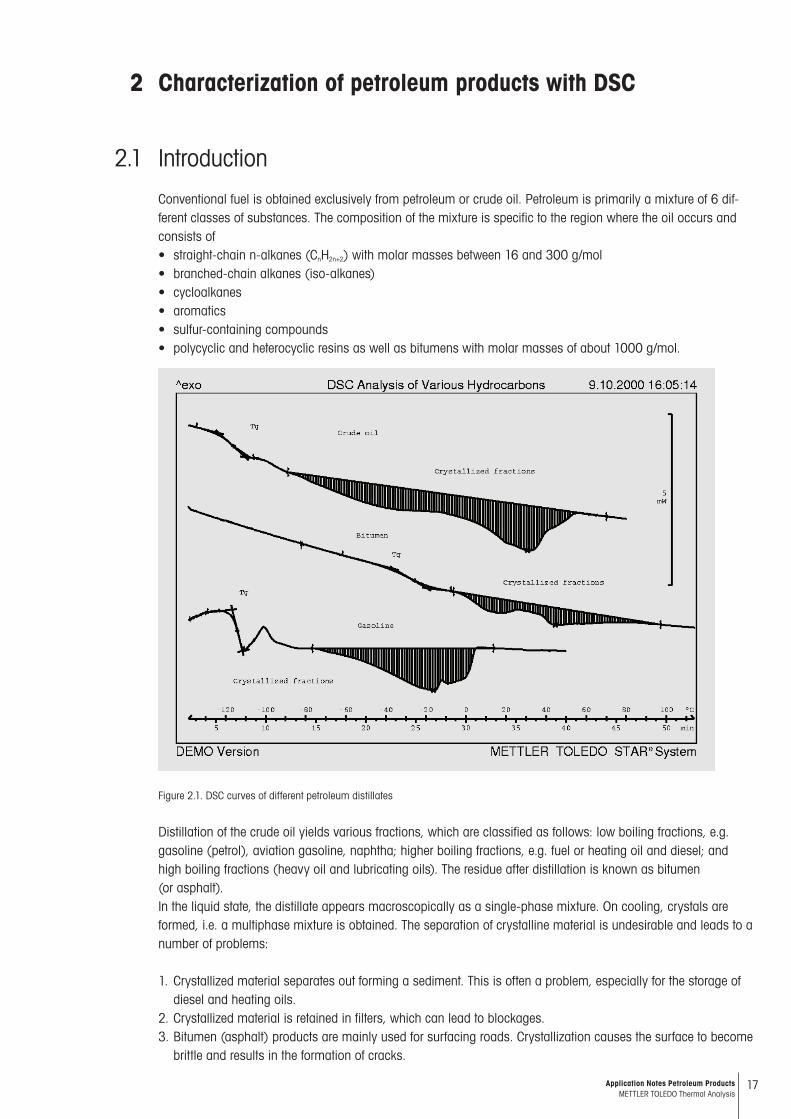
Figure 2.1. DSC curves of different petroleum distillates

Distillation of the crude oil yields various fractions, which are classified as follows: low boiling fractions, e.g. gasoline (petrol), aviation gasoline, naphtha; higher boiling fractions, e.g. fuel or heating oil and diesel; and high boiling fractions (heavy oil and lubricating oils). The residue after distillation is known as bitumen (or asphalt). In the liquid state, the distillate appears macroscopically as a single-phase mixture. On cooling, crystals are formed, i.e. a multiphase mixture is obtained. The separation of crystalline material is undesirable and leads to a number of problems:

1. Crystallized material separates out forming a sediment. This is often a problem, especially for the storage of diesel and heating oils.

2. Crystallized material is retained in filters, which can lead to blockages.3. Bitumen (asphalt) products are mainly used for surfacing roads. Crystallization causes the surface to become

brittle and results in the formation of cracks.


Char

acte

rizat

ion

of p

etro

leum

pro

duct

s w

ith D

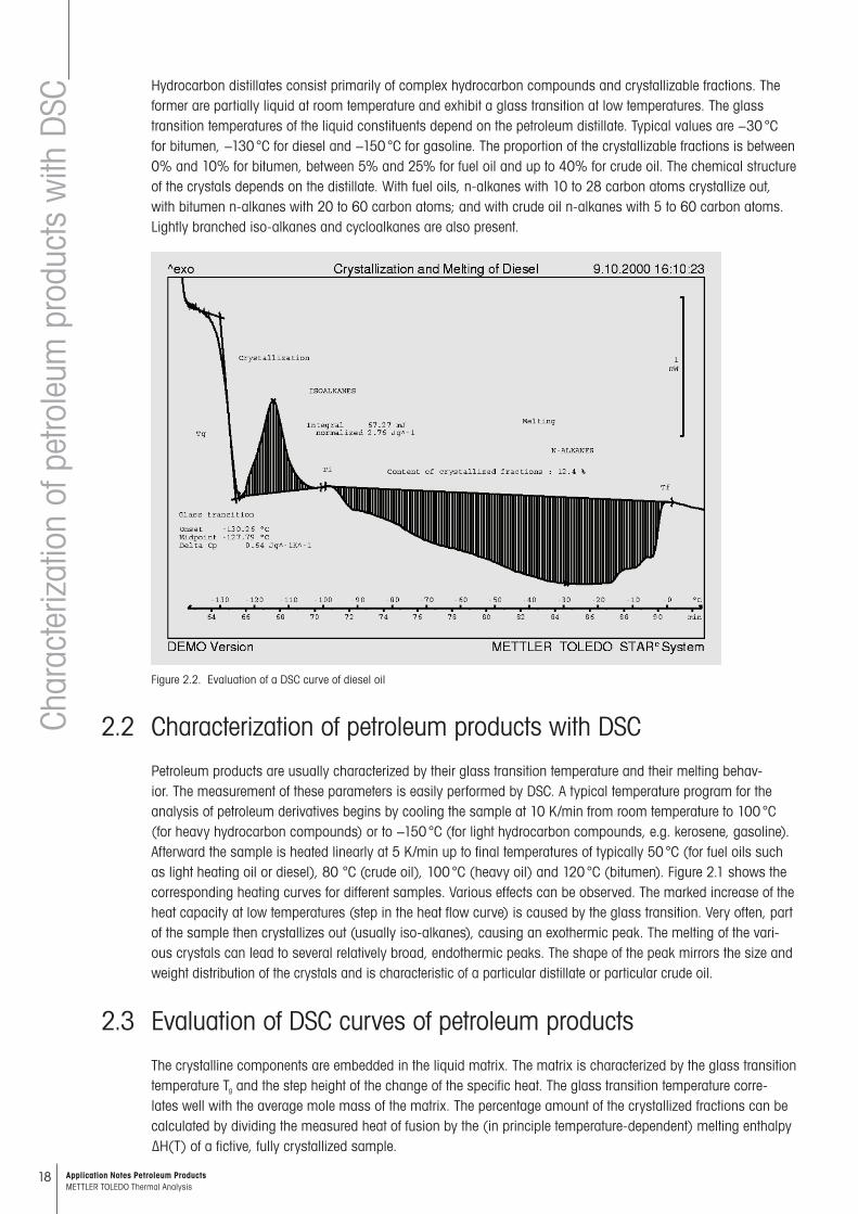
SCHydrocarbon distillates consist primarily of complex hydrocarbon compounds and crystallizable fractions. The former are partially liquid at room temperature and exhibit a glass transition at low temperatures. The glass transition temperatures of the liquid constituents depend on the petroleum distillate. Typical values are −30 °C for bitumen, −130 °C for diesel and −150 °C for gasoline. The proportion of the crystallizable fractions is between 0% and 10% for bitumen, between 5% and 25% for fuel oil and up to 40% for crude oil. The chemical structure of the crystals depends on the distillate. With fuel oils, n-alkanes with 10 to 28 carbon atoms crystallize out, with bitumen n-alkanes with 20 to 60 carbon atoms; and with crude oil n-alkanes with 5 to 60 carbon atoms. Lightly branched iso-alkanes and cycloalkanes are also present.

Figure 2.2. Evaluation of a DSC curve of diesel oil

2.2 Characterization of petroleum products with DSC

Petroleum products are usually characterized by their glass transition temperature and their melting behav-ior. The measurement of these parameters is easily performed by DSC. A typical temperature program for the analysis of petroleum derivatives begins by cooling the sample at 10 K/min from room temperature to 100 °C (for heavy hydrocarbon compounds) or to −150 °C (for light hydrocarbon compounds, e.g. kerosene, gasoline). Afterward the sample is heated linearly at 5 K/min up to final temperatures of typically 50 °C (for fuel oils such as light heating oil or diesel), 80 °C (crude oil), 100 °C (heavy oil) and 120 °C (bitumen). Figure 2.1 shows the corresponding heating curves for different samples. Various effects can be observed. The marked increase of the heat capacity at low temperatures (step in the heat flow curve) is caused by the glass transition. Very often, part of the sample then crystallizes out (usually iso-alkanes), causing an exothermic peak. The melting of the vari-ous crystals can lead to several relatively broad, endothermic peaks. The shape of the peak mirrors the size and weight distribution of the crystals and is characteristic of a particular distillate or particular crude oil.

2.3 Evaluation of DSC curves of petroleum products

The crystalline components are embedded in the liquid matrix. The matrix is characterized by the glass transition temperature Tg and the step height of the change of the specific heat. The glass transition temperature corre-lates well with the average mole mass of the matrix. The percentage amount of the crystallized fractions can be calculated by dividing the measured heat of fusion by the (in principle temperature-dependent) melting enthalpy ∆H(T) of a fictive, fully crystallized sample.


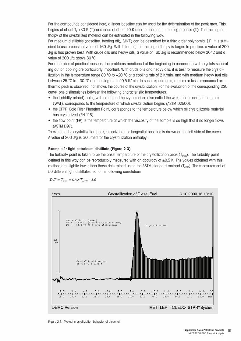
For the compounds considered here, a linear baseline can be used for the determination of the peak area. This begins at about Tg +30 K (Ti) and ends at about 10 K after the end of the melting process (Tf). The melting en-thalpy of the crystallized material can be estimated in the following way.For medium distillates (gasoline, heating oil), ∆H(T) can be described by a third order polynomial [1]. It is suffi-cient to use a constant value of 160 J/g. With bitumen, the melting enthalpy is larger. In practice, a value of 200 J/g is has proven best. With crude oils and heavy oils, a value of 160 J/g is recommended below 30 °C and a value of 200 J/g above 30 °C.For a number of practical reasons, the problems mentioned at the beginning in connection with crystals separat-ing out on cooling are particularly important. With crude oils and heavy oils, it is best to measure the crystal-lization in the temperature range 80 °C to −20 °C at a cooling rate of 2 K/min; and with medium heavy fuel oils, between 25 °C to −30 °C at a cooling rate of 0.5 K/min. In such experiments, a more or less pronounced exo-thermic peak is observed that shows the course of the crystallization. For the evaluation of the corresponding DSC curve, one distinguishes between the following characteristic temperatures:• the turbidity (cloud) point, with crude and heavy oils often also called the wax appearance temperature

(WAT), corresponds to the temperature at which crystallization begins (ASTM D2500).• the CFPP, Cold Filter Plugging Point, corresponds to the temperature below which all crystallizable material

has crystallized (EN 116).• the flow point (FP) is the temperature at which the viscosity of the sample is so high that it no longer flows

(ASTM D97).To evaluate the crystallization peak, a horizontal or tangential baseline is drawn on the left side of the curve. A value of 200 J/g is assumed for the crystallization enthalpy.

Example 1: light petroleum distillate (Figure 2.3)The turbidity point is taken to be the onset temperature of the crystallization peak (Tonset). The turbidity point defined in this way can be reproducibly measured with an accuracy of ±0.5 K. The values obtained with this method are slightly lower than those determined using the ASTM standard method (TASTM). The measurement of 50 different light distillates led to the following correlation:

WAT = Tonset = 0.98·TASTM −3.6

Figure 2.3. Typical crystallization behavior of diesel oil


For the determination of the CFPP value, the analysis of 40 light petroleum products gave the following correla-tion between the temperature at which 0.45% of the crystallizable material has crystallized out (Tc(0.45%)) and the CFPP determined according to EN 116:

Tc(0.45%) = 1.01·TCFPP EN 106 − 0.85.

For the determination of the flow point we found the optimum correlation to be:

Tc(1%) = 1.02·Tflow point ASTM − 0.28

Here, Tc(1%) is the temperature at which 1% of the crystallizable fractions has crystallized out. [2].

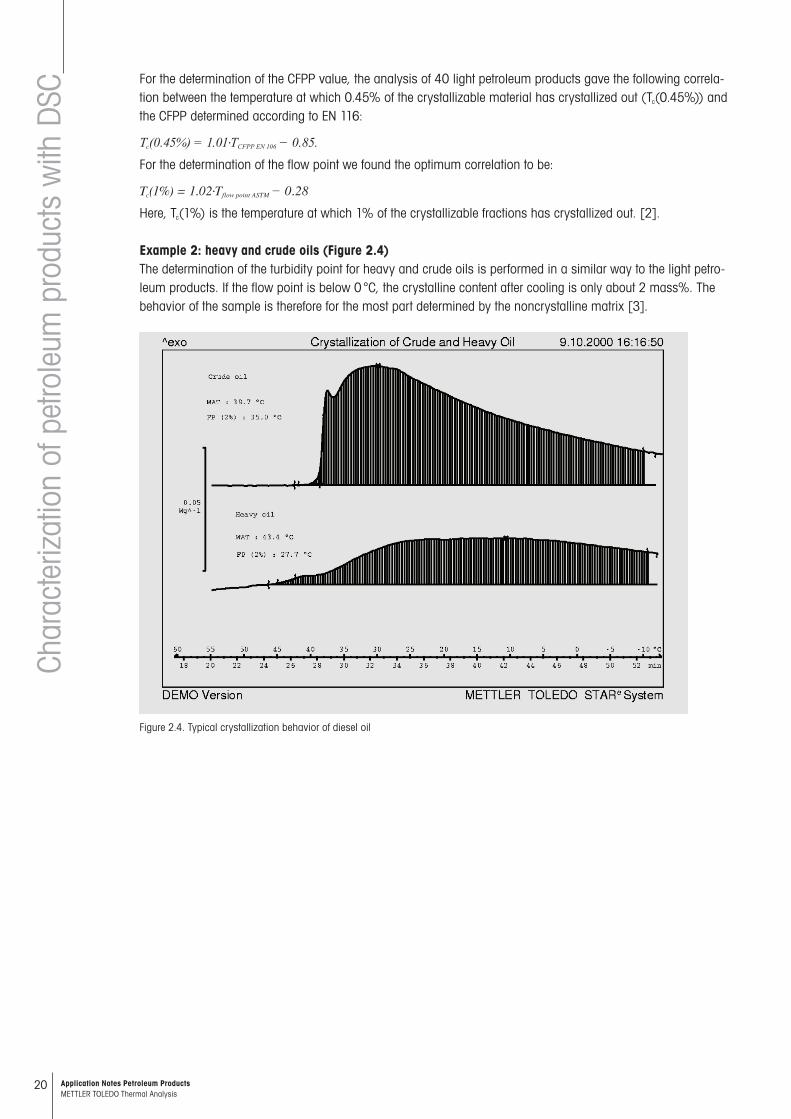
Example 2: heavy and crude oils (Figure 2.4)The determination of the turbidity point for heavy and crude oils is performed in a similar way to the light petro-leum products. If the flow point is below 0 °C, the crystalline content after cooling is only about 2 mass%. The behavior of the sample is therefore for the most part determined by the noncrystalline matrix [3].

Figure 2.4. Typical crystallization behavior of diesel oil

Char

acte

rizat

ion

of p

etro

leum

pro

duct

s w

ith D

SC


2.4 Conclusions

DSC measurements allow a rapid and reliable characterization of extremely different types of petroleum prod-ucts. The glass transition temperature and melting behavior provide important information on the quality of petroleum derivatives. In addition, the origin of a sample of unknown petroleum can be determined because the measured curves are characteristic of the petroleum, i.e. they are “fingerprints”. Cooling experiments yield impor-tant practical information on the crystallization behavior of petroleum derivatives.

AuthorJ. M. Létoffé, Laboratoire de Thermodynamique Appliqué, INSA 69621, Villeurbanne Cedex

Literature[1] F. Bosselet, Thèse Saint Etienne n°008 (1984)[2] P. Claudy, J.M. Létoffé, B. Neff, B. Damin, FUEL, 65 (1986) 861–864[3] J.M. Létoffé, P. Claudy, M.V. Kok, M. Garcin, J.L. Volle, FUEL, 74 (6) (1995) 810–817


Oxi

dativ

e st

abili

ty o

f pet

role

um o

il fra

ctio

ns

3.1 Introduction

The determination of the oxidative induction temperature is a rapid method for assessing the stability of petroleum oil fractions. The same method can be used to measure the effectiveness of stabilizers. Besides this, aging processes can also be investigated. Standardized isothermal methods are often used instead of dynamic methods (e.g. ASTM D 5483 and ASTM E 1858). Analysis under high pressures of oxygen prevents the vaporiza-tion of volatile components and increases the rate of oxidation, thereby shortening the measurement time [1, 2].The DSC measurements provide a comparison of the products with respect to their stability in oxygen.

3.2 Samples and measurement parameters

Diesel oils of the following petroleum fractions: Light (LGO), Light Cycle (LCGO), Light Vacuum (LVGO), Vacuum1 (VGO1), Vacuum2 (VGO2), Vacuum3 (VGO3) and Kerosine.

Measuring cell DSC27HP / TC15Crucible Aluminum 40 µl, with pierced lid (1 mm hole)DSC measurement Put the measuring cell under an atmosphere of oxygen and heatfrom 40 °C to 150 °C

at 20 K/min (to save time), then continue up to 350 °C at 5 K/min. The measurement is automatically terminated when the value of the exothermic DSC

signal reaches 10 mW (the combustion peak is not of interest).Atmosphere Oxygen at 3 MPa, no purge gas.

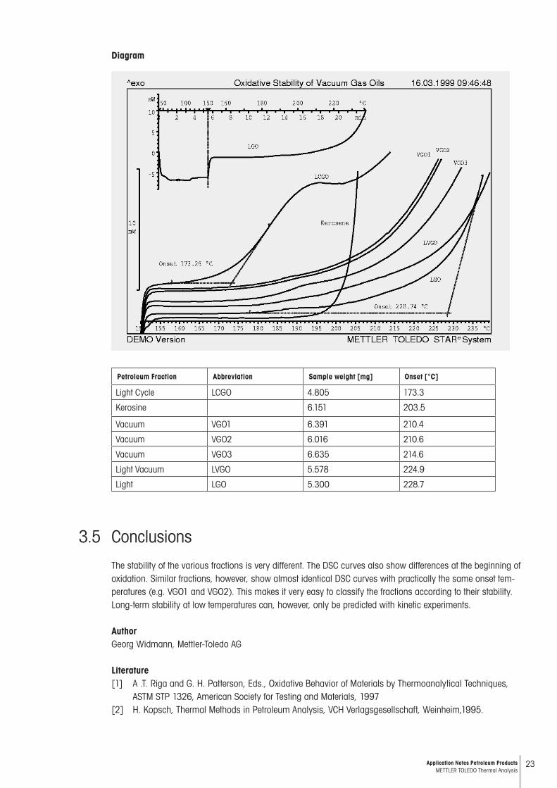
3.3 Interpretation

The high pressure of oxygen prevents any premature vaporization so that, on heating, a deflection in the DSC curve is caused only by a change in the specific heat of the sample and no other thermal effects are observed before the beginning of oxidation. The full curve for light diesel oil (LGO) is shown in the upper diagram; the change in the heating rate at 150 °C is marked with a vertical line. The lower diagram shows the measurements of all the samples from 150 °C onwards. The curves are arranged so that they can be seen clearly. The tangents used for the evaluation are drawn for the samples of lowest and highest stability. The abbreviations refer to the petroleum fractions mentioned above.

3.4 Evaluation

The oxidative stability is compared by determining the temperature at which oxidation begins (onset). This value is considered to be characteristic of the sample. It is measured as the point of intersection of the horizontal tangent of the baseline before oxidation and the tangent at the steepest part of the DSC curve:

3 Oxidative stability of petroleum oil fractions


Diagram

Petroleum Fraction Abbreviation Sample weight [mg] Onset [°C]

Light Cycle LCGO 4.805 173.3

Kerosine 6.151 203.5

Vacuum VGO1 6.391 210.4

Vacuum VGO2 6.016 210.6

Vacuum VGO3 6.635 214.6

Light Vacuum LVGO 5.578 224.9

Light LGO 5.300 228.7

3.5 Conclusions

The stability of the various fractions is very different. The DSC curves also show differences at the beginning of oxidation. Similar fractions, however, show almost identical DSC curves with practically the same onset tem-peratures (e.g. VGO1 and VGO2). This makes it very easy to classify the fractions according to their stability. Long-term stability at low temperatures can, however, only be predicted with kinetic experiments.

AuthorGeorg Widmann, Mettler-Toledo AG

Literature[1] A .T. Riga and G. H. Patterson, Eds., Oxidative Behavior of Materials by Thermoanalytical Techniques,

ASTM STP 1326, American Society for Testing and Materials, 1997[2] H. Kopsch, Thermal Methods in Petroleum Analysis, VCH Verlagsgesellschaft, Weinheim,1995.


Det

erm

inat

ion

of th

e N

oack

eva

pora

tion

loss

of l

ubric

ants

4.1 Abstract

For quality and environmental reasons, lubricants for engines and other applications must only exhibit a low evaporation rate. The loss of volatile components from an oil increases its viscosity and leads to increased oil consumption, coking and wear. The Noack method is a widely used standard test method for measuring the evaporation loss from lubricating oils. According to the ILSAC GF-3 and API-SL specifications the evaporation loss must not be greater than 15%.The ASTM standard test method D6375 for the determination of the evaporation loss of lubricating oils by the Noack method [1] uses thermogravimetric analysis, TGA. This method yields the same results as other standard test methods (e.g. ASTM D5800 [2], DIN 51581-1 [3], JPI-5S-41-93 [4]). This article describes how the Noack evaporation loss is determined in comparison to a reference oil sample using TGA.

4.2 Introduction

The increase in the usable lifetime of lubricants coupled with faster oil circulation rates, longer oil change inter-vals and lower lubricant consumption means that lubricants are subjected to greater stress. Higher temperatures coupled with smaller oil volumes and higher performance lead to a constant increase in the demands placed on the performance and quality of the lubricants. To ensure that the lubricants are properly used, they must be properly specified and classified.The specifications describe the physical properties of engine oils such as the viscosity, evaporation loss and shear stability. Performance behavior is also tested in engine tests. This includes wear protection and cleanli-ness as well as the influence on fuel consumption and the changes in the engine oil during operation due to viscosity changes (thickening). The classification is provided by organizations such as ILSAC, API or SAE (see the table of acronyms).

AcronymsAPI: American Petroleum InstituteASTM: ASTM International, originally known as the American Society for Testing and MaterialsDIN: Deutsches Institut für Normung (German Institute for Standardization)ILSAC: International Lubricant Standardization and Approval CommitteeJPI: Petroleum Association of JapanSAE: SAE International, Society of Automotive Engineers

One of the commonly used specifications is the evaporation loss. The low molecular mass constituents of an engine oil, which consists of fractions of different hydrocarbons with different chain lengths and molecular masses, can evaporate under increased thermal stress. This usually leads to an increase in the viscosity of the lubricant. At the same time, the solubility of the additives in the base oil is affected. The evaporation is important for all lubricant groups (e.g. also for synthetic oils) if they are used at higher tem-peratures. For example with engine oils, evaporation losses can occur through high temperatures at the piston rings and elsewhere. These losses lead to undesirable oil thickening and increased oil consumption.

4.3 The Noack evaporation loss test according to ASTM D6375

The Noack test to quantitatively determine the evaporation loss of oils under standard conditions was introduced many years ago. For example, the DIN 51581 [3] test method measures the evaporation loss over a period of one hour at 250 °C under vacuum (2 mbar).

4 Determination of the Noack evaporation loss of lubricants by TGA


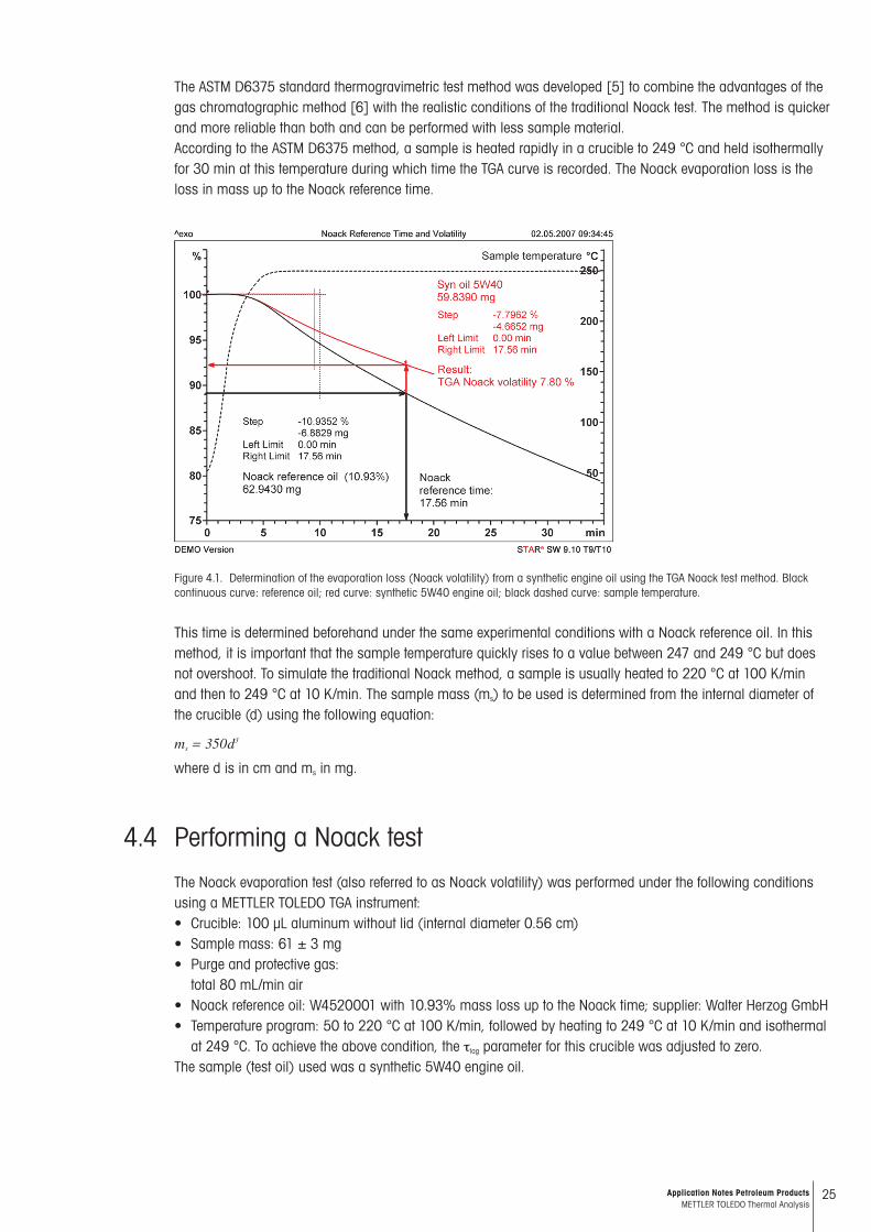
The ASTM D6375 standard thermogravimetric test method was developed [5] to combine the advantages of the gas chromatographic method [6] with the realistic conditions of the traditional Noack test. The method is quicker and more reliable than both and can be performed with less sample material. According to the ASTM D6375 method, a sample is heated rapidly in a crucible to 249 °C and held isothermally for 30 min at this temperature during which time the TGA curve is recorded. The Noack evaporation loss is the loss in mass up to the Noack reference time.

Figure 4.1. Determination of the evaporation loss (Noack volatility) from a synthetic engine oil using the TGA Noack test method. Black continuous curve: reference oil; red curve: synthetic 5W40 engine oil; black dashed curve: sample temperature.

This time is determined beforehand under the same experimental conditions with a Noack reference oil. In this method, it is important that the sample temperature quickly rises to a value between 247 and 249 °C but does not overshoot. To simulate the traditional Noack method, a sample is usually heated to 220 °C at 100 K/min and then to 249 °C at 10 K/min. The sample mass (ms) to be used is determined from the internal diameter of the crucible (d) using the following equation:

ms = 350d3

where d is in cm and ms in mg.

4.4 Performing a Noack test

The Noack evaporation test (also referred to as Noack volatility) was performed under the following conditions using a METTLER TOLEDO TGA instrument:• Crucible: 100 µL aluminum without lid (internal diameter 0.56 cm)• Sample mass: 61 ± 3 mg• Purge and protective gas:

total 80 mL/min air• Noack reference oil: W4520001 with 10.93% mass loss up to the Noack time; supplier: Walter Herzog GmbH• Temperature program: 50 to 220 °C at 100 K/min, followed by heating to 249 °C at 10 K/min and isothermal

at 249 °C. To achieve the above condition, the tlag parameter for this crucible was adjusted to zero.The sample (test oil) used was a synthetic 5W40 engine oil.


Figure 4.1 shows the TGA curve (black line) of the reference oil. The Noack reference time is 17.56 min; this is the time at which the certified loss of 10.93% is reached (see the black arrows). The TGA curve of the sample is shown as the red curve. After 17.56 min the loss is read off as 7.80% (see red arrows): the synthetic 5W40 engine oil thus has a Noack evaporation loss of 7.8%. This is often given in the oil specification simply as NOACK 7.8%.According to ASTM D6375, the repeatability with 8% loss is about 1% for two determinations by the same labo-ratory, and the reproducibility is about 1.4% for two determinations by different laboratories.According to ASTM D6375, the TGA furnace must be regularly heated out. The method recommends that this is done after about ten determinations. The furnace should be heated to 1000 °C without a crucible and held iso-thermally at this temperature for about 5 min. The air gas flow is left at about 80 mL/min.

4.5 Conclusions

Over the past years, the demands placed on lubricants in many application areas have changed significantly. Thermal oxidation stability, low tendency to evaporate and their influence on our natural and working environ-ments have become very important. The innovative development of modern lubricants and their proper applica-tion have far-reaching economical consequences. Lubricants (base liquid and additives) that have been opti-mized for the different tasks, for example with low evaporation losses,• save energy• reduce service intervals• minimize wear• increase engine service life• increase oil change intervals (lifetime) and result in considerable economical savings. The determination of the evaporation loss by thermogravimetry is therefore an important step in the qualification of lubricant. The METTLER TOLEDO TGA system with sample robot and automated evaluation provides high sample throughput and rapid pass/fail assessment of the oil in question.

AuthorDr. Rudolf Riesen, Mettler-Toledo AG

Literature[1] ASTM D6375 Standard Test Method for Evaporation Loss of Lubricating Oils by Thermogravimetric Analyzer

(TGA) Noack Method.[2] ASTM D-5800 Test Method for Evaporation Loss of Lubricating Oils by the Noack Method.[3] DIN 51581-1, 2003-02 Determination of the evaporative loss of petroleum products by the Noack

method – Part 1 (original in German).[4] JPI-5S-41-93 Determination of Evap-oration Loss of Engine Oils (Noack Method).[5] E. F. de Paz, C. B. Sneyd – The Thermogravimetric Noack Test: a Precise, Safe and Fast Method for

Measuring Lubricant Volatility, Subjects in Engine Oil Rheology and Tribology, SP1209, International Fall Fuel and Lubricants Meeting, San Antonio 1996, available also as SAE Technical Papers, Document Number: 962035.

[6] DIN 51581-2, 1997-05 Determination of the evaporation loss of petroleum products by gas chromatography – Part 2 (original in German).

Det

erm

inat

ion

of th

e N

oack

eva

pora

tion

loss

of l

ubric

ants


5 Rapid thermogravimetric analysis of coal

5.1 Introduction

The quantitative determination of moisture, volatile compounds, chemically bound carbon, and ash content has long been used to determine the quality and economic value of different types of coal. High ash content is unde-sirable for the operation of thermal power stations because inert material increases transport and waste disposal costs, and also means that the heat exchangers have to be cleaned more frequently. To make sure that assays can be properly compared, the analysis procedures have been standardized and described in many standard methods [1–10].Quite early on, measurement routines were developed for thermogravimetric instruments that enabled faster and more automated analyses to be performed. These techniques have been compared with the standard manual methods [11–14]. TGA (thermogravimetric analysis) is, however, also very useful for coal research, e.g. to compare combustion profiles or to determine the nature of volatile components with TGA-MS. Even the lime deposits (fur) formed in hot water systems have been investigated with TGA [15]. The determination of moisture, volatile content, soot, ash or fillers is also required for other applications. Analo-gous to the analysis of coal, a standardized thermo gravimetric procedure is nowadays used to determine the content of elastomers, thermoplastics and thermosets, as well as lubricants [16, 17]. Conversely, procedures developed for the determination of carbon black in rubber [17] are used for the analysis of brown coal, lignite and or other renewable fossil fuels [e.g. 18].

5.2 Speeding up the TGA procedure

As already indicated, the standard methods for coal analysis are laborious and often time-consuming.To determine the moisture content exactly, the measurement is usually started at room temperature, or slightly above. This leads to long cooling times before the next sample can be measured, which in turn limits the throughput of samples.The METTLER TOLEDO STARe system allows the analysis time to be reduced by half compared to the ASTM E1131 standard method. In this case, the measurement is started directly at 110 °C (or even higher), which means the otherwise long cooling time down to 30 °C is avoided. The moisture is, however, still accurately measured - the weight loss up to the start is automatically measured by determining the starting weight on reaching 110 °C. This is done by measuring the weight of the sample and the crucible during the sample preparation, which is in fact normal in the manual procedure [1–10]. Buoyancy effects are compensated in the TGA measurement by sub-traction of a blank curve.Besides this, oxygen is used instead of air, resulting in much shorter combustion times. One must of course make sure that coal particles are not blown out of the crucible by the rapid generation of gas. This can manifest itself for example in widely differing measurement values for the ash content. As with all analytical methods, it is essential that the coal samples are homogeneous and representative if one, for example, wants to characterize one hundred tons of coal. Vaporization, degassing and combustion proceed more rapidly when shallow, open crucibles are used and small sample weights are analyzed.


Rapi

d th

erm

ogra

vim

etric

ana

lysi

s of

coa

l 5.3 Experimental details

A METTLER TOLEDO TGA/SDTA851e with the small furnace (up to 1100 °C) was used for the measurements. The system was automated with a TSO800RO sample robot and a TSO800GC1 gas controller for gas switching.The balance was purged with 40 ml/min of nitrogen as protective gas. During the measurement, first 80 ml/min of nitrogen, and afterward 80 ml/min of oxygen were used as reactive gas.

The following samples were used as examples for coal analysis:1. Coal A with a particle size of 65 µm to 90 µm,2. Coal B with a particle size up to 1 mm,3. Coke, finely powered, manufactured from petroleum oil.

Unless otherwise specified, alumina crucibles (30 µl) were filled with about 20 mg of coal powder. During weighing-in, the crucible weight and the sample weight were noted and entered in the software program. Immediately after weighing-in, the special aluminum lid was placed on the crucible to prevent contamination of the sample and any large change in moisture content during the waiting time. The lid is removed by the sample robot during measurement.At the end of the measurement, the measuring cell automatically cools down to the starting temperature. The blank curve is automatically subtracted and the evaluation macro-program calculates the weight loss immediately after the measurement is finished.

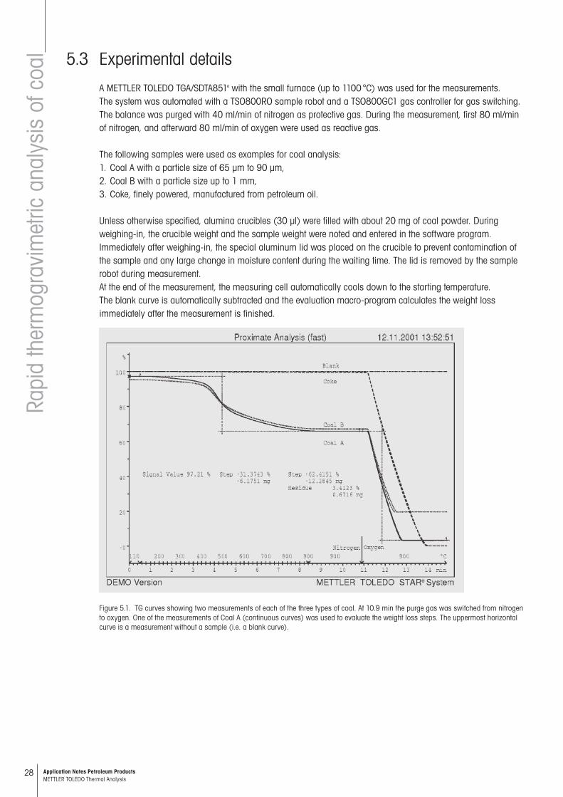
Figure 5.1. TG curves showing two measurements of each of the three types of coal. At 10.9 min the purge gas was switched from nitrogen to oxygen. One of the measurements of Coal A (continuous curves) was used to evaluate the weight loss steps. The uppermost horizontal curve is a measurement without a sample (i.e. a blank curve).


5.4 Results

Fast methodFigure 5.1 shows the TGA curves of the coal analyses performed with the fast method described above. The measurement conditions were chosen as follows:Under nitrogen: 110 °C for 0.5 min, then heating at 100 K/min to 900 °C and held at this temperature for 2.5 minutes. The system was then purged with oxygen for the following 4 minutes (furnace atmosphere is made up of 80 ml/min O2 and 40 ml/min N2).The blank curve was measured in the same way before the measurement series with an empty crucible.For all measurements (including the blank curve), the weight of the crucible is also entered in the software in addition to the sample weight, i.e. the total weight is determined directly after weighing-in. After insertion of the sample by the sample robot and the equilibration of the temperature at 110 °C (automatic “settling”), the total weight is determined at this instant with the first measurement point. The difference between this and the sample weight before the mea-surement yields the dry content (or the amount of moisture evolved). The starting weight is given by the Signal Value (Figure 5.1) at the beginning of the normalized TGA curve. This means that drying or moisture uptake during the wait-ing time up to the actual measurement has no influence on the original moisture content. However, especially with very moist coal samples, the use of an aluminum lid is recommended as described in the experimental section.In the first 30 seconds, the TG curves are practically horizontal with a loss of less than 3 µg (this corresponds to 0.01%), proving that drying is complete at the beginning of the measurement. The curves are also horizontal at the end of the isothermal phase at 900 °C because degassing and combustion have finished.The measured values are summarized in Table 5.1. The reproducibility is shown by the standard deviation and how well the measurement curves coincide. The slight differences in combustion rates are caused by small dif-ferences in the sample weights, e.g. with Coal B 19.801 mg as opposed to 21.547 mg (see Figure 5.1).In routine operation, the analysis including evaluation takes approximately 36 minutes; of this, about 15 minutes is for the actual measurement. The assay according to ASTM E1131 takes about 60 minutes because somewhat longer isothermal times are necessary and because an additional cooling time of 10 minutes is needed to reach 30 °C.As Table 1 shows, the corresponding mean values for both methods are very close. The differences are less than the reproducibility of >0.3% given in the manual methods [5–7]. It is noticeable that there is a tendency for the fast method to yield higher moisture values and lower volatile contents. This can be explained by a loss due to drying of about 0.4% with the ASTM method [16] before the actual measurement. This can only be prevented if the weighed-in sample is immediately measured.The comparatively high standard deviations with Coal B are also worth noting. This is also apparent in the man-ually weighed residues. Measurements in crucibles with alumina lids (with a hole) and in taller crucibles (70 µl) showed that the differences cannot however be explained through too rapid combustion with “firework-like” ejection of material (“sparkling coal”). Better grinding and homogenization of the sample however reduced the standard deviations by a factor three. The reason is the inhomogeneity of this coal sample. This underlines the necessity of good sample preparation. The comparison of the two coal types A and B show this very clearly.

Table 5.1. Comparison of the contents measured using the fast method with the values according to the ASTM E1131 standard. In each case, the mean values (M) and the corresponding standard deviations (SD) are calculated from three measurements. The residue is deter-mined by manually reweighing when the measurement is completed as specified in the standards [2 and 6]. All the values refer to the initial sample weight.


5.5 Conclusions

The assay of moisture, volatile content, carbon and ash in coal and coke using TGA is a standardized routine method. The time required for the method can be shortened by up to 50% without affecting the accuracy by using the METTLER TOLEDO STARe system and adapting the temperature program. In automated operation, this allows at least 35 analyses to be performed per day.The TGA curves show whether degassing and combustion are complete. This is necessary in order to optimize the method and for the control of routine measurements. Thermogravimetry, in addition, allows drying and com-bustion behavior to be investigated and different coal types to be characterized.Inhomogeneous samples must be well ground to achieve a high degree of repro ducibility. If necessary, larger amounts of sample can be measured thermogravi metrically in 900 µl crucibles.

AuthorDr. Rudolf Riesen, Mettler-Toledo AG

Literature 1. DIN 51718 Analysis of solid fuels - determination of water content and analysis moisture (in German). 2. DIN 51719 Analysis of solid fuels - determination of ash content. (in German) 3. DIN 51720 Analysis of solid fuels - determination of the content of volatile components. (in German) 4. ASTM D3172 Standard Practice for Proximate Analysis of Coal and Coke. 5. ASTM D3173 Standard Test Method for Moisture in the Analysis Sample of Coal and Coke. 6. ASTM D3174 Standard Test Method for Ash in the Analysis Sample of Coal and Coke. 7. ASTM D3175 Standard Test Method for Volatile Matter in the Analysis Sample of Coal and Coke. 8. ISO 11722 as well as BS 1016-104.1 Methods for analysis and testing of coal and coke. Proximate analy-

sis. Determination of moisture content of the general analysis test sample. 9. ISO 562 as well as BS 1016-104.3 Methods for analysis and testing of coal and coke. Proximate analysis.

Determination of volatile matter content.10. ISO 1171 as well as BS 1016-104.4 Methods for analysis and testing of coal and coke. Proximate analysis.

Determination of ash content.11. Richard L. Fyans, “Rapid Characteriza tion of Coal by Thermogravimetric and Scanning Calorimetric Analy-

sis”, Presentation at the 28th Pittsburgh Conference in Cleveland, Ohio, March (1977).12. John W. Cumming, Joseph McLaughlin, “The thermogravimetric behavior of coal”, Thermochimica Acta,

57 (1982) 253–272.13. F. S. Sadek, A. Y. Herrell, “Proximate analysis of solid fossil fuels by thermo gravimetry”, American Labora-

tory, March (1984) 75–78.14. Danny E. Larkin, “The development of a standard method”, ASTM STP 997 “Compositional analysis by

thermo gravimetry”, C.M. Earnest, Ed., American Society for Testing and Materials, Philadelphia (1988) 28–37.

15. Paul Baur, “Thermogravimetry speeds up proximate analysis of coal”, Power, March (1983) 91–93.16. ASTM E1131 Standard Test Method for Compositional Analysis by Thermo gravimetry.17. ISO 9924 Rubber and rubber products. Determination of the composition of vulcanizates and uncured

compounds by thermogravimetry.18. M.C. Mayoral, et. al., “Different approaches to proximate analysis by thermogravimetry analysis”, Thermo-

chimica Acta, 370 (2001) 91–97.

Rapi

d th

erm

ogra

vim

etric

ana

lysi

s of

coa

l


6 Determination of oxidation stability by pressure-dependent OIT measurements

6.1 Introduction

The determination of the oxidation induction time (OIT) is a method frequently used to estimate the oxidation stability of materials. This is done by first heating the sample to a sufficiently high temperature under inert conditions (purging the DSC cell with nitrogen). After a brief thermal equilibration time, the purge gas is switched from nitrogen to oxy-gen. If the temperature has been chosen correctly there is no immediate change in the DSC signal. However, after a certain induction time, the exothermic oxidation reaction begins. The OIT is the time at which the onset of the oxidation reaction occurs measured from the point when the gas is switched from nitrogen to oxygen. The OIT depends very much on the current chemical state of a material. For example, chemical aging causes a significant decrease in the measured OIT.

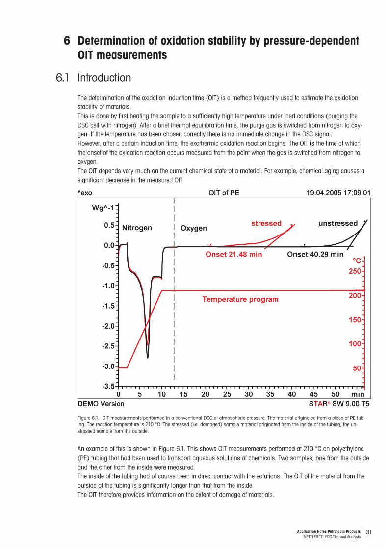
Figure 6.1. OIT measurements performed in a conventional DSC at atmospheric pressure. The material originated from a piece of PE tub-ing. The reaction temperature is 210 °C. The stressed (i.e. damaged) sample material originated from the inside of the tubing, the un-stressed sample from the outside.

An example of this is shown in Figure 6.1. This shows OIT measurements performed at 210 °C on polyethylene (PE) tubing that had been used to transport aqueous solutions of chemicals. Two samples, one from the outside and the other from the inside were measured. The inside of the tubing had of course been in direct contact with the solutions. The OIT of the material from the outside of the tubing is significantly longer than that from the inside. The OIT therefore provides information on the extent of damage of materials.


D

eter

min

atio

n of

oxi

datio

n st

abili

ty 6.2 Experimental details

The measurements described in this study on the pressure dependence of OIT were performed using the new high pressure DSC (HP DSC827e). The oxygen pressure and gas flow were set using a pressure and flow regula-tor. The gas flow was 40 mL/min and the oxygen pressure set to different values in the range 0.1 MPa to 10 MPa (1 to 100 bar). Since gas switching in pressure measurements is not always so easy, the oxygen pressure was set at room temperature and the sample heated rapidly at 50 K/min to the reaction temperature.The chemiluminescence measurements were performed in an HP DSC827e using a CCD camera and the relevant accessories [1].

6.3 Pressure dependence of OIT

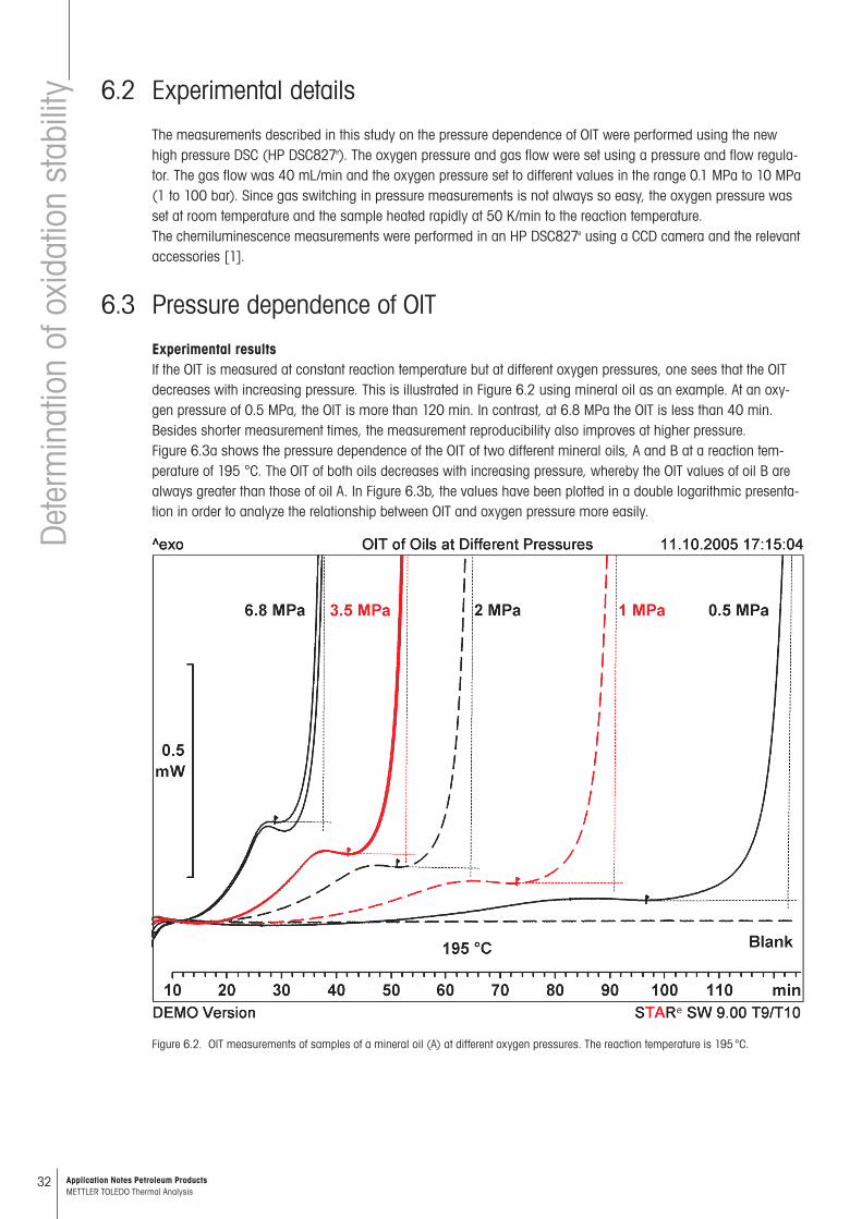
Experimental resultsIf the OIT is measured at constant reaction temperature but at different oxygen pressures, one sees that the OIT decreases with increasing pressure. This is illustrated in Figure 6.2 using mineral oil as an example. At an oxy-gen pressure of 0.5 MPa, the OIT is more than 120 min. In contrast, at 6.8 MPa the OIT is less than 40 min. Besides shorter measurement times, the measurement reproducibility also improves at higher pressure. Figure 6.3a shows the pressure dependence of the OIT of two different mineral oils, A and B at a reaction tem-perature of 195 °C. The OIT of both oils decreases with increasing pressure, whereby the OIT values of oil B are always greater than those of oil A. In Figure 6.3b, the values have been plotted in a double logarithmic presenta-tion in order to analyze the relationship between OIT and oxygen pressure more easily.

Figure 6.2. OIT measurements of samples of a mineral oil (A) at different oxygen pressures. The reaction temperature is 195 °C.


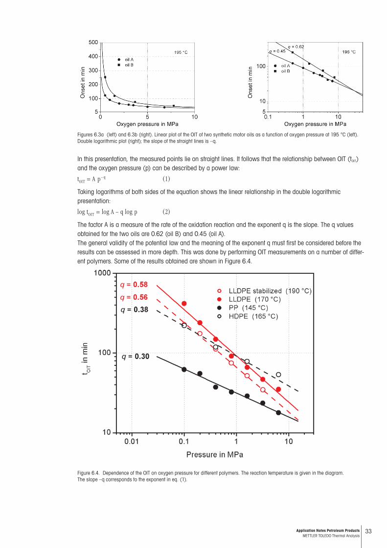
Figures 6.3a (left) and 6.3b (right). Linear plot of the OIT of two synthetic motor oils as a function of oxygen pressure at 195 °C (left). Double logarithmic plot (right); the slope of the straight lines is –q.

In this presentation, the measured points lie on straight lines. It follows that the relationship between OIT (tOIT) and the oxygen pressure (p) can be described by a power law:

Taking logarithms of both sides of the equation shows the linear relationship in the double logarithmic presentation:

The factor A is a measure of the rate of the oxidation reaction and the exponent q is the slope. The q values obtained for the two oils are 0.62 (oil B) and 0.45 (oil A). The general validity of the potential law and the meaning of the exponent q must first be considered before the results can be assessed in more depth. This was done by performing OIT measurements on a number of differ-ent polymers. Some of the results obtained are shown in Figure 6.4.

Figure 6.4. Dependence of the OIT on oxygen pressure for different polymers. The reaction temperature is given in the diagram. The slope –q corresponds to the exponent in eq. (1).


Different reaction temperatures were chosen for each polymer so that the OIT values were all in a convenient time frame (between 20 and 300 min). This facilitated the analysis of the pressure dependence of OIT for the materials tested. The diagram shows that in double logarithmic presentation the relationship is linear for all the polymers investigated. The exponent q here lies between 0.6 (linear low-density polyethylene, LLDPE), and 0.3 (polypropylene, PP).

6.4 Interpretation of the results

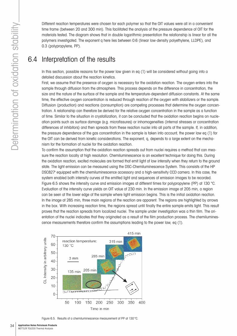
In this section, possible reasons for the power law given in eq (1) will be considered without going into a detailed discussion about the reaction kinetics.First, we assume that the presence of oxygen is necessary for the oxidation reaction. The oxygen enters into the sample through diffusion from the atmosphere. This process depends on the difference in concentration, the size and the nature of the surface of the sample and the temperature-dependent diffusion constants. At the same time, the effective oxygen concentration is reduced through reaction of the oxygen with stabilizers or the sample. Diffusion (production) and reactions (consumption) are competing processes that determine the oxygen concen-tration. A relationship can therefore be derived for the relative oxygen concentration in the sample as a function of time. Similar to the situation in crystallization, it can be concluded that the oxidation reaction begins on nucle-ation points such as surface damage (e.g. microfissures) or inhomogeneities (internal stresses or concentration differences of inhibitors) and then spreads from these reaction nuclei into all parts of the sample. If, in addition, the pressure dependence of the gas concentration in the sample is taken into account, the power law eq (1) for the OIT can be derived from kinetic considerations. The exponent, q, depends to a large extent on the mecha-nism for the formation of nuclei for the oxidation reaction.To confirm the assumption that the oxidation reaction spreads out from nuclei requires a method that can mea-sure the reaction locally at high resolution. Chemiluminescence is an excellent technique for doing this. During the oxidation reaction, excited molecules are formed that emit light of low intensity when they return to the ground state. The light emission can be measured using the DSC-Chemiluminescence System. This consists of the HP DSC827e equipped with the chemiluminescence accessory and a high-sensitivity CCD camera. In this case, the system enabled both intensity curves of the emitted light and sequences of emission images to be recorded.Figure 6.5 shows the intensity curve and emission images at different times for polypropylene (PP) at 130 °C. Evaluation of the intensity curve yields an OIT value of 230 min. In the emission image at 205 min, a region can be seen at the lower edge of the sample where light emission begins. This is the initial oxidation reaction. In the image at 285 min, three main regions of the reaction are apparent. The regions are highlighted by arrows in the box. With increasing reaction time, the regions spread until finally the entire sample emits light. This result proves that the reaction spreads from localized nuclei. The sample under investigation was a thin film. The ori-entation of the nuclei indicates that they originated as a result of the film production process. The chemilumines-cence measurements therefore confirm the assumptions leading to the power law, eq (1).

Figure 6.5. Results of a chemiluminescence measurement of PP at 130 °C.

Det

erm

inat

ion

of o

xida

tion

stab

ility


6.5 Assessment of experimental results

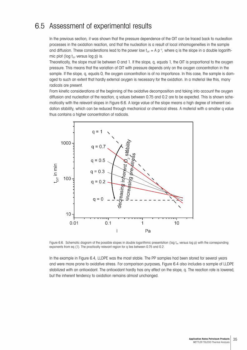
In the previous section, it was shown that the pressure dependence of the OIT can be traced back to nucleation processes in the oxidation reaction, and that the nucleation is a result of local inhomogeneities in the sample and diffusion. These considerations lead to the power law tOIT = A p–q, where q is the slope in a double logarith-mic plot (log tOIT versus log p) is.Theoretically, the slope must lie between 0 and 1. If the slope, q, equals 1, the OIT is proportional to the oxygen pressure. This means that the variation of OIT with pressure depends only on the oxygen concentration in the sample. If the slope, q, equals 0, the oxygen concentration is of no importance. In this case, the sample is dam-aged to such an extent that hardly external oxygen is necessary for the oxidation. In a material like this, many radicals are present. From kinetic considerations at the beginning of the oxidative decomposition and taking into account the oxygen diffusion and nucleation of the reaction, q values between 0.75 and 0.2 are to be expected. This is shown sche-matically with the relevant slopes in Figure 6.6. A large value of the slope means a high degree of inherent oxi-dation stability, which can be reduced through mechanical or chemical stress. A material with a smaller q value thus contains a higher concentration of radicals.

Figure 6.6. Schematic diagram of the possible slopes in double logarithmic presentation (log tOIT versus log p) with the corresponding exponents from eq (1). The practically relevant region for q lies between 0.75 and 0.2.

In the example in Figure 6.4, LLDPE was the most stable. The PP samples had been stored for several years and were more prone to oxidative stress. For comparison purposes, Figure 6.4 also includes a sample of LLDPE stabilized with an antioxidant. The antioxidant hardly has any effect on the slope, q. The reaction rate is lowered, but the inherent tendency to oxidation remains almost unchanged.


6.6 Conclusions

The pressure dependence of OIT obeys a power law. The exponent q is mainly influenced through oxygen diffu-sion processes and radical formation in the material under test. Materials with small exponents tend to oxidize more readily than those with large exponents. The power law dependence of OIT on pressure presupposes a nu-cleation process before the reaction. This means that the oxidation does not begin throughout the entire sample, but just in a few isolated regions in the sample where conditions are favorable for diffusion (e.g. microfissures) or where there is a greater concentration of radicals. This nucleation mechanism in the oxidation reaction can be measured by chemiluminescence.The pressure dependence of OIT provides additional information on the stability, previous damage, and inherent tendency for oxidation of materials.It is important to remember when performing OIT measurements that the geometry of samples plays an impor-tant role because of its influence on diffusion processes. For this reason, it is best to use very thin samples with defined surface areas.The author would like to thank his colleagues Dr. R. Riesen, M. Zappa and Dr M. Schubnell for valuable help and discussions.

AuthorDr. Jürgen Schawe, Mettler-Toledo AG

Literature1. Thermal Analysis UserCom 20, Mettler-Toledo AG, (2004).

Det

erm

inat

ion

of o

xida

tion

stab

ility


7 Standards for petrochemicals with respect to thermal analysis

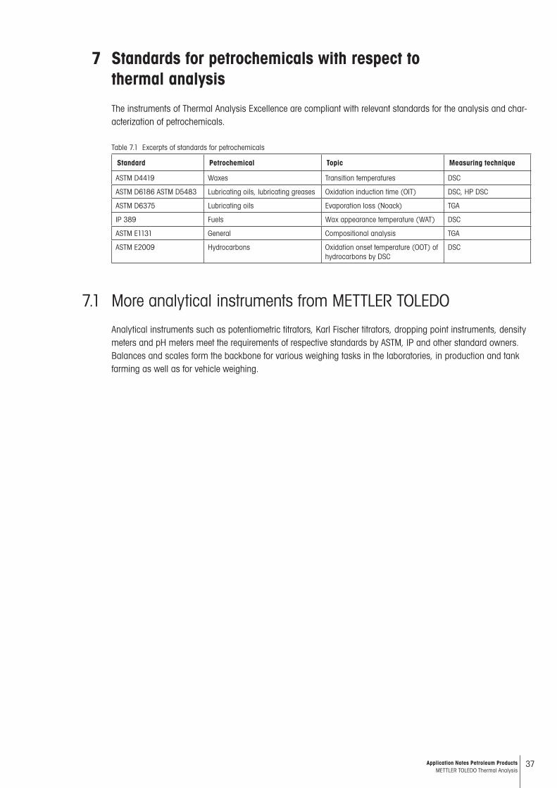
The instruments of Thermal Analysis Excellence are compliant with relevant standards for the analysis and char-acterization of petrochemicals.

Table 7.1 Excerpts of standards for petrochemicals

Standard Petrochemical Topic Measuring technique

ASTM D4419 Waxes Transition temperatures DSC

ASTM D6186 ASTM D5483 Lubricating oils, lubricating greases Oxidation induction time (OIT) DSC, HP DSC

ASTM D6375 Lubricating oils Evaporation loss (Noack) TGA

IP 389 Fuels Wax appearance temperature (WAT) DSC

ASTM E1131 General Compositional analysis TGA

ASTM E2009 Hydrocarbons Oxidation onset temperature (OOT) of hydrocarbons by DSC

DSC

7.1 More analytical instruments from METTLER TOLEDO

Analytical instruments such as potentiometric titrators, Karl Fischer titrators, dropping point instruments, density meters and pH meters meet the requirements of respective standards by ASTM, IP and other standard owners.Balances and scales form the backbone for various weighing tasks in the laboratories, in production and tank farming as well as for vehicle weighing.


Mor

e In

form

atio

n

METTLER TOLEDO offers you valuable support and services to keep you informed about new developments and help you expand your knowledge and expertise, including:

News on Thermal AnalysisInforms you about new products, applications and events. www.mt.com/ta-news

HandbooksWritten for thermal analysis users with background information, theory and practice, useful tables of material properties and many interesting applications. www.mt.com/ta-handbooks

The following Collected Applications Handbooks can be purchased as color-printed books:

TutorialThe Tutorial Kit handbook with twenty-two well-chosen application examples and the corresponding test substances provides an excellent introduction to thermal analysis techniques and is ideal for self-study. www.mt.com/ta-handbooks

UserComOur popular, biannual technical customer magazine, where users and specialists publish applications from different fields. www.mt.com/ta-usercoms

ApplicationsIf you have a specific application question, you may find the answer in the application database. www.mt.com/ta-applications

WebinarsWe offer web-based seminars (webinars) on different topics. After the presentation, you will have the opportunity to discuss any points of interest with specialists or with other participants. www.mt.com/ta-webinars (Live Webinars) www.mt.com/ta-ondemand (On Demand Webinars) www.mt.com/ta-etraining (Web-based)

TrainingClassroom training is still one of the most effective ways to learn. Our User Training Courses will help you get the most from your equipment. We offer a variety of one-day theory and hands-on courses aimed at familiarizing you with our thermal analysis sys-tems and their applications. www.mt.com/ta-training

8. For More Information

Title Order Number Title Order Number

Thermal Analysis in Practice 51725244 Elastomers Vol. 1 51725057

Validation in Thermal Analysis 51725141 Elastomers Vol. 2 51725058

Food 51725004 Elastomers Vol. 1 and Vol. 2 51725061

Pharmaceuticals 51725006 Thermosets Volume 1 51725067

Thermoplastics 51725002 Thermosets Volume 2 51725068

EGA Evolved Gas Analysis 51725056 Thermosets Volume 1 + 2 51725069

Title Order Number Title Order Number

Tutorial Kit (handbook only) 51709920 Tutorial Kit (handbook and test samples) 51140879

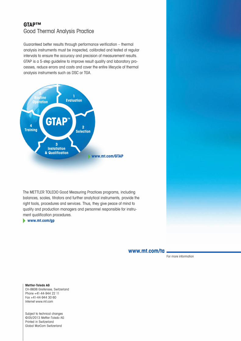
www.mt.com/ta

Mettler-Toledo AGCH-8606 Greifensee, SwitzerlandPhone +41-44-944 22 11Fax +41-44-944 30 60Internet www.mt.com

Subject to technical changes©05/2013 Mettler-Toledo AGPrinted in SwitzerlandGlobal MarCom Switzerland

Guaranteed better results through performance verification – thermal analysis instruments must be inspected, calibrated and tested at regular intervals to ensure the accuracy and precision of measurement results. GTAP is a 5-step guideline to improve result quality and laboratory pro-cesses, reduce errors and costs and cover the entire lifecycle of thermal analysis instruments such as DSC or TGA.

For more information

GTAP™ Good Thermal Analysis Practice

GTAPTM

1Evaluation

2Selection

3Installation

& Qualification

5Routine

Operation

4Training

The METTLER TOLEDO Good Measuring Practices programs, including balances, scales, titrators and further analytical instruments, provide the right tools, procedures and services. Thus, they give peace of mind to quality and production managers and personnel responsible for instru-ment qualification procedures. www.mt.com/gp

www.mt.com/GTAP

Documents

Thermal Analysis - METTLER TOLEDO Balances & … Notes Petroleum Products 5 METTLER TOLEDO Thermal Analysis Preface Thermal analysis is one of the oldest analysis techniques. Throughout