PORE PRESSURE AND FRACTURE PRESSURE MODELLING WITH- OFFSET WELL DATA

AND ITS APPLICATION TO-SURFACE CASING DESIGN OF A DEVELOPMET WELL

DEEP PANUKE GAS POOL OFFSHORE NOVA SCOTIA

By

Theja Kankanamge

Submitted in partial fulfillment of the requirements

for the degree of Master of Engineering

At

Dalhousie University

Halifax, Nova Scotia

August 21, 2013

© Copyright by Theja Kankanamge

1

ACKNOWLEDGEMENTS

First I would like to thank our petroleum engineering Department Chair Dr.Michael Pegg for

facilitating us to gain more knowledge of petroleum engineering during the study period.

Special thanks to my project supervisor Dr.Mae Seto for in partial fulfillment of the

requirements for the degree of Master of Engineering her patience and guidance throughout my

graduate studies. Her knowledge and experience provided tremendous benefit to growth in my

career and academic development.

I would like to give very sincere thanks to Mrs. Mary Jean Verrall from Geoscience Research

Centre Canada-Nova Scotia Offshore Petroleum Board for allowing the continued use of this data set to

perform this study.

Also I would like to thank current drilling engineering lecturer Mumni Amadu for his support and

guidance given.

I would like to thank Mrs. Nancy White for helping to find out the data for the formation from

Geoscience Research Centre Canada-Nova Scotia Offshore Petroleum Board

2

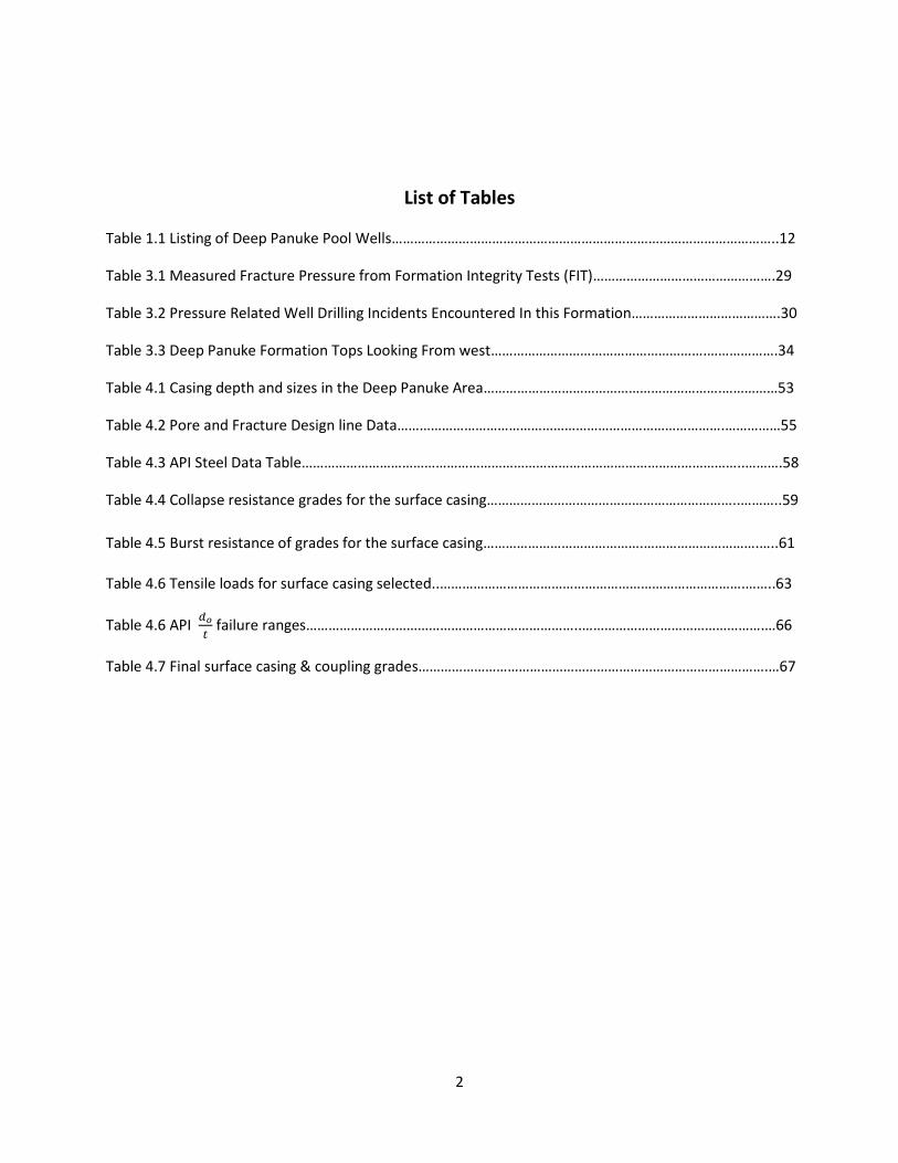
List of Tables

Table 1.1 Listing of Deep Panuke Pool Wells…………………………………………………………………………………………..12

Table 3.1 Measured Fracture Pressure from Formation Integrity Tests (FIT)………………………………………….29

Table 3.2 Pressure Related Well Drilling Incidents Encountered In this Formation………………………………….30

Table 3.3 Deep Panuke Formation Tops Looking From west………………………………………………….……………….34

Table 4.1 Casing depth and sizes in the Deep Panuke Area……………………………………………………….……………53

Table 4.2 Pore and Fracture Design line Data…………………………………………………………………………….……………55

Table 4.3 API Steel Data Table………………………………………………………………………………………………………..……….58

Table 4.4 Collapse resistance grades for the surface casing…………………………………………………………..………..59

Table 4.5 Burst resistance of grades for the surface casing…………………………………….………………………….…..61

Table 4.6 Tensile loads for surface casing selected..……………………………………………………………………….……..63

Table 4.6 API 𝑑𝑜

𝑡 failure ranges………………………………………………………………..………………………………………….…66

Table 4.7 Final surface casing & coupling grades………………………………………………………………………………….…67

3

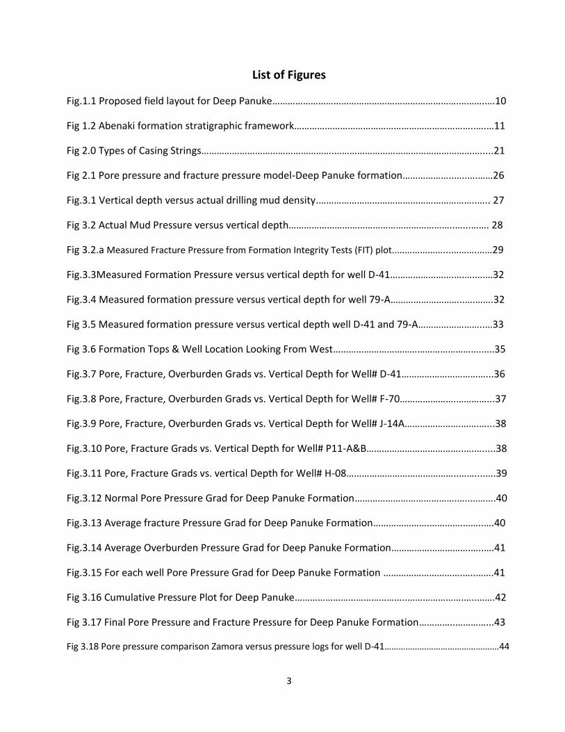
List of Figures

Fig.1.1 Proposed field layout for Deep Panuke……………………………………………………………….……….….10

Fig 1.2 Abenaki formation stratigraphic framework……………………………………………………………..….…11

Fig 2.0 Types of Casing Strings…………………………………………….………………………………………………….....21

Fig 2.1 Pore pressure and fracture pressure model-Deep Panuke formation………………..…..….……26

Fig.3.1 Vertical depth versus actual drilling mud density.……………………………………………………..….. 27

Fig 3.2 Actual Mud Pressure versus vertical depth………………………………………………………..…...……. 28

Fig 3.2.a Measured Fracture Pressure from Formation Integrity Tests (FIT) plot..………………...……….……29

Fig.3.3Measured Formation Pressure versus vertical depth for well D-41…………………….….….….…32

Fig.3.4 Measured formation pressure versus vertical depth for well 79-A………………………..….…….32

Fig 3.5 Measured formation pressure versus vertical depth well D-41 and 79-A……………………..…33

Fig 3.6 Formation Tops & Well Location Looking From West…………………………………………………..….35

Fig.3.7 Pore, Fracture, Overburden Grads vs. Vertical Depth for Well# D-41……………………………...36

Fig.3.8 Pore, Fracture, Overburden Grads vs. Vertical Depth for Well# F-70………………….…………...37

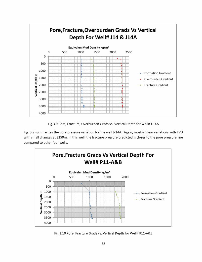
Fig.3.9 Pore, Fracture, Overburden Grads vs. Vertical Depth for Well# J-14A………………….…….…...38

Fig.3.10 Pore, Fracture Grads vs. Vertical Depth for Well# P11-A&B………………………………..….….....38

Fig.3.11 Pore, Fracture Grads vs. vertical Depth for Well# H-08……………………………………..……....….39

Fig.3.12 Normal Pore Pressure Grad for Deep Panuke Formation………………………………….…..……….40

Fig.3.13 Average fracture Pressure Grad for Deep Panuke Formation………………….………….……..….40

Fig.3.14 Average Overburden Pressure Grad for Deep Panuke Formation………………………….…..….41

Fig.3.15 For each well Pore Pressure Grad for Deep Panuke Formation ………………………….…..…….41

Fig 3.16 Cumulative Pressure Plot for Deep Panuke……………………………………..………………….…..…….42

Fig 3.17 Final Pore Pressure and Fracture Pressure for Deep Panuke Formation…………..…………...43

Fig 3.18 Pore pressure comparison Zamora versus pressure logs for well D-41……………………………………….…44

4

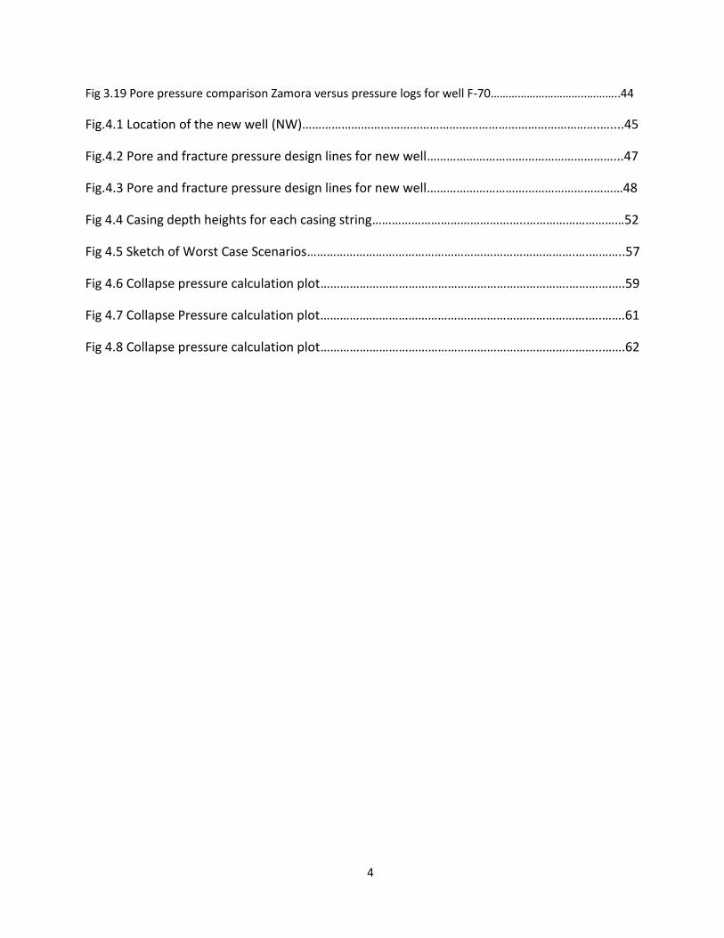
Fig 3.19 Pore pressure comparison Zamora versus pressure logs for well F-70…………………………..………..44

Fig.4.1 Location of the new well (NW)……………………………………………………………………………….…....45

Fig.4.2 Pore and fracture pressure design lines for new well…………………………………………………...47

Fig.4.3 Pore and fracture pressure design lines for new well……………………………………………………48

Fig 4.4 Casing depth heights for each casing string………………………………………..…………………………52

Fig 4.5 Sketch of Worst Case Scenarios……………………………………………………………………….….………..57

Fig 4.6 Collapse pressure calculation plot………………………………………………………………….………….….59

Fig 4.7 Collapse Pressure calculation plot……………………………………………………………………….….…….61

Fig 4.8 Collapse pressure calculation plot…………………………………………………………………………..…….62

5

ABSTRACT

The purpose of this project is to develop a pore pressure and fracture pressure prediction strategy

for Deep Panuke area and apply the proposed model to design a surface casing of a development well in the

formation. To achieve this offset well data from eight wells in the pool will be reviewed, analysed and predict

an analytical model. The final pore and fracture pressure model developed will be helpful for future

developments in the pool when they are drilling new developments wells.

In this study an analytical method is used to predict the pore pressure and fracture pressure model,

here the all the raw data collected will be transformed into a form where interpretations can be made. Using

the real-time drilling data the model is verified.

One Pore pressure and one fracture pressure prediction strategy correlations that can be applied to

the formation will be discussed.

When the pore pressure model is finalized that will be used to design the surface casing of a

development well in the formation.

The fracture pressure and pore pressure model can be used for future development of the Deep

Panuke Formation.

6

NOMENCLATURE

BHA - Bottom Hole Assembly

TVD -True Vertical Depth (m)

MD -Measured Depth (m)

ECD - Equivalent Circulating Density (kg/m³)

min -minimum

max -maximum

LWD -Logging While Drilling

MWD -Measured While Drilling

MW -Mud Weight or Mud density (kg/m³)

ROP -Rate of Penetration (m/hr)

TD -Total Depth (m)

TVD -Total Vertical Depth (m)

WOB -Weight on bit (daN)

RPM -Revolution per minute

Pf - Formation Pressure (kPa)

Pff -Fracture Pressure (kPa)

ᵛ - Poison ratio

ρ - Drilling fluid density (kg/m³)

ρe -Equivalent Mud Density (kg/m³)

C -Constant

σo -Overburden pressure (kPa)

σ’ -Effective stress (kPa)

D&A -Drilled and abandoned

σ’a -Effective horizontal stress (kPa)

σ’o -Effective overburden stress (kPa)

Vp -Compressional velocity (m/s)

Vs -Shear Velocity (m/s)

Yp -Joint yield strength (kgf)

σy -Yield stress (kgf)

RFT -Repeat formation test

MDT -Modular dynamic test

σ -Total stress (kPa)

7

Table of Contents

Acknowledgements…………………………………………………………………………………………………………………….…..…...1

List of Tables…………………………………………………………………………………………………………………..………..……………2

List of Figures…………………………………………………………………………………………………………………….................….3

Abstract………………………………………………………………………………………………………………………..……………...........5

Nomenclature.………………………………………………………………………………………………………………………….…….......6

1. Introduction …………………………………………………………………………………………………………..…….………………..…9

1.1.1 Introduction……………………………………………………………………………………………………………………...9 1.1.2 Project Objectives…………………………………………..…………………………………………….………………….9 1.2 Deep Panuke Formation Overview & Drilling History10 1.2.1Geology of Deep Panuke Formation……………………………………………………………....................11 1.2.2 Pool Discovery and Delineation History…………………………………………………………................12 1.3 Overview of the Project………………………………………………………………………………………………......12

2. Literature Review……………………………………………………………………………………………………..……………….…...13

2.1 Pore Pressure and Fracture Pressure Prediction Strategies….…………………………………………….….13

2.1.0 Introduction……………………………………………………………………………………….……………….13 2.1.1 Analytical Interpretation of Field Data……………………………….…………..…………………..14 …2.1.1.1 Overview of analytical Interpretation of field Data……………………….……………….14

2.1.1.2 Basic Concepts In interpretation of field Data…………………………………………….…..15 2.1.2 Estimation of Formation Pressure While Drilling……………………………..…................ 17 2.1.2.1 Analysis of Drilling Performance Data………………………………………..……………….....17 2.1.3 Prediction of Fracture Pressure…………………………………………………..….……………..…..…19 2.1.3.1 Ben Eaton Fracture Gradient Prediction…………………………………..………………….....19 2.2 Casing Design Literature Review………………………………………………………………….………………....….20

2.2.1Introduction………………………………………………………………………………………………….........20 2.2.2 Types of Casings and their functions……………………………………………….....……….…..…21 2.2.3 Design Criteria……………………………………………………………………………………………………..22 2.2.3.1 Burst Mechanism…………………………………………………………………………................…22 2.2.3.2 Collapse Mechanism……………………………………………………………….……….……….…...23 2.2.3.3 Tension Mechanism………………………………………………………………..………….….........24 2.2.3.4 Temperature effects……………………………………………………………….……...............…24 2.2.3.5 Biaxial Loading………………………………………………………………………..………………...…..24 2.2.3.6 Sour Service…………………………………………………………………………………………….……..25 2.2.3.7 Time Scenario…………………………………………………………………………….……………..…..25 2.2.3.7 Casing Wear……………………………………………………………………………..………………..….25 2.2.3.8 Casing Landing effect…………………………..…………………………………………………………25

3. Deep Panuke Offset Well Data Review………………………………………………………………………………...……...27

3.1 Drilling Data Review……………………………………………………………………………………………………….…..27

8

3.2 Measured Pressure Data Review ……………………………………………………………………………….……...31 3.3 Prediction of Pore Pressure & Fracture Pressure for the Pool………………………….………….....…35 3.4 Pore Pressure calculation from Zamora Method for Deep Panuke Formation……………………44

4. Casing Design Calculation………………………………………………………………..……………………….……………..…….45

4.1Location of the New Well (NW)…………………………………………………………………….……………….…...45

4.2 Basic Design Considerations …………………………………………………………………………………………...….46

4.3 Casing Setting Depth Calculations and Factors Considered…………………. ………………………….....47

4.4 Assumptions, Calculations and Steps Followed ……………………………………………………………....….48

4.5 To check the pipe sticking test for the production casing……………………………….……………….....49

4.6 Surface Casing String Settling Depth……………………………………………………………………………….…..49

4.7 Conductor Pipe Setting Depth………………………………………………………………………………………..…...51

4.8 Casing String Sizes Calculations and Factors Considered ………………………………………………..…..52

4.8.1 Factors affecting the selection of Casing Sizes

4.9 Selection of Casing Weight Grade and Couplings……………………………………………..…………………56

4.9.1Collapse Failure………………………………………………………………………………………..……………….….56

4.9.2 Burst Failure……………………………………………………………………………………………………….……..…59

4.9.3 Tension Failure…………………………………………………………………………………………………….….…..62

4.9.3.1 Pressure Testing and Shock Loading affecting the tension failure……………….……….…63

4.9.4 Biaxial Effects………………………………………………………………………………………………….……….…..64

4.10 Final Selection of the Surface Casing String……………………………………………..……………..……...67

5. Conclusions………………………………………………………….…………………………………………………………….……......68

5.1 Pore Pressure and Fracture Pressure Prediction……………………………………………………...……..….68 5.2 Casing Design ………………………………………………………………………………………………………..………..…69

References………………………………………………………………………………………………………………………………………....70

Appendix A1: Deep Panuke Well Recaps…………………………………………………………………………………………....71

Appendix A2: Measured well data in Deep Panuke formation………………………………………………….….…….78

Appendix A3: Pore, Fracture, Overburden pressure from well pressure logs …………………………………….80

Appendix A4: Zamora Method well data tables…………………………………………………………..…………….….....85

9

1. Introduction

1.1.1 Introduction

Accurate prediction of the sub-surface pore pressures and fracture gradients is a necessary

requirement for safe, economical and efficient drilling of the wells required to explore and produce oil and

natural gas reserves. One of the most important parameters to determine the reliability and success of a

casing design is the pore pressure. For normally pressurized areas pore pressure can be predicted easily.

For an abnormally pressurized formation, it is more difficult and that much more important to know the pore

pressure. Clear interpretation of the formation pressure is needed for the drilling plan to choose casing points

and to design a casing that allows the well to be drilled effectively and maintain well control during drilling

and completion operations. If accurate pore and fracture gradients are used at the design stage well control

events such as fluid kicks, lost circulation, surface blowouts and underground blowouts can be prevented.

The offset well data consisted of eight wells in the Deep Panuke gas pool and nearby block to create

an accurate pore pressure and fracture pressure model for the area. Analytical interpretation of field data

was used to predict pore pressure and fracture pressure for the formation. The pore pressure predicted

graph can be used as a reference in the Deep Panuke formation for future well drillings.

1.1.2 Project Objectives

The main objective of this project was to develop a pore pressure and fracture pressure model for the Deep

Panuke formation and a surface casing design for a development well. Offset well data consisted of eight

wells in the Deep Panuke gas pool nearby block are studied to create the model ,using the model and the

API design standard practice surface casing design of a development well is carried out.

10

1.2 Deep Panuke Formation Overview and Drilling History

The Deep Panuke natural gas field was discovered in 1998 by PanCanadian Petroleum Limited, now

EnCana Corporation. EnCana holds a majority working interest in, and is the operator of, the field located

approximately 250km southeast of Halifax, Nova Scotia, on the Scotia Shelf. Deep Panuke underlies the

Cohasset and Panuke oil fields which produced a total of 7.1 million cubic meters (44 million barrels)of oil

between 1992 and 1999.

Deep Panuke is considered a sour gas reservoir with raw gas containing approximately 0.18%

hydrogen sulphide. The acid gas produced is injected to the nearby Mississauga formation. The production

design sales gas throughput for the project was 300 MMscf/d.,Recoverable sales gas resources are estimated

to be within 390Bcf to 892Bcf with a mean of 632Bcf.The resource forecast shows the probable field life

ranging from 8 years to 17.5years.The topside is designed for a life of 20years and the structures for 25years.

Fig.1.1 Proposed field layout for Deep Panuke

(CNSOPB Deep Panuke Development Plan Decision Report 2007)

1.2.1Geology of Deep Panuke Formation

11

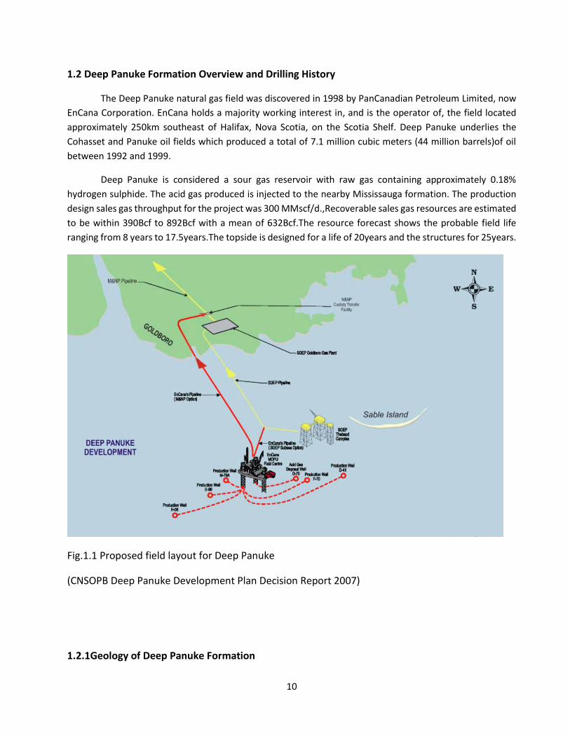
The Deep Panuke reservoir is located near the top of the Late Jurassic Abenaki formation. The

Abenaki is dominated by limestone of various depositional environments recording an ancient and long lived

reef margin like the modern Great Barrier Reef complex offshore eastern Australia(Fig1.2).The reservoir

lithology are leached and fractured lime stones and dolostones with various types and ranges of porosities

and permeabilities.

Fig 1.2 Abenaki formation stratigraphic framework

(EnCana Deep Panuke Project report-2, 2006)

12

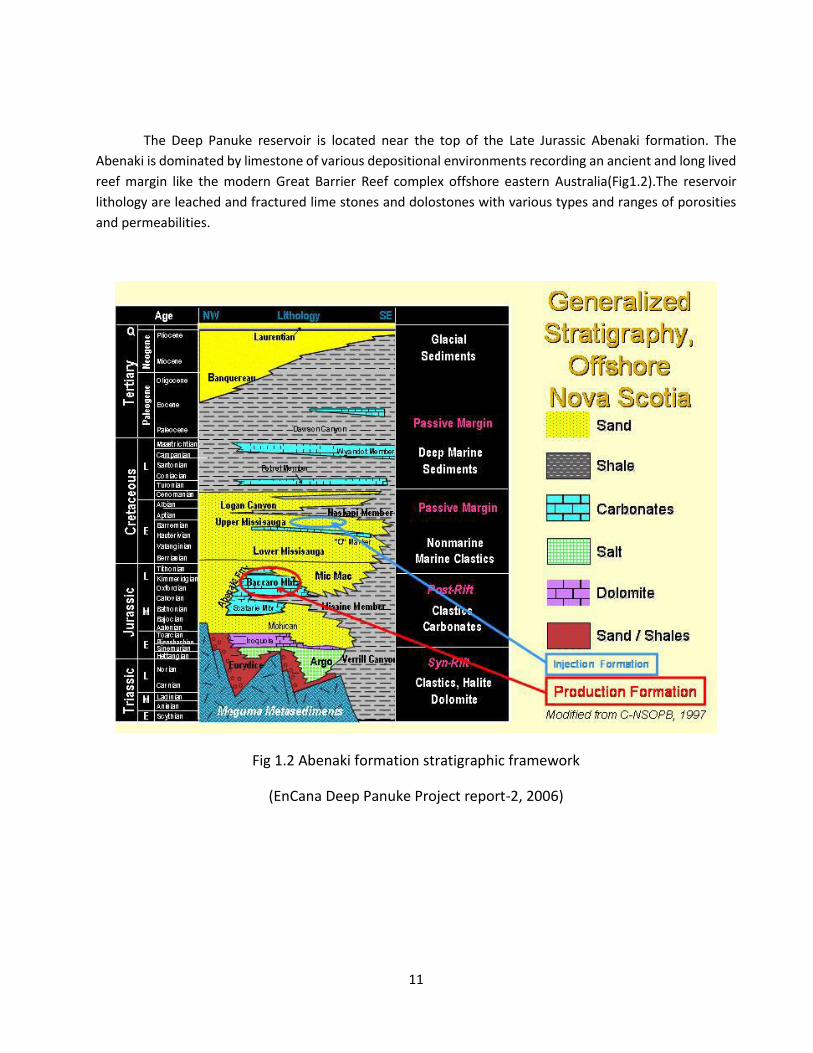
1.2.2 Pool Discovery and Delineation History

The Panuke PP-3C well is the discovery well for the Deep Panuke gas pool drilled in 1996.Table 1.1

summarizes the list of wells, history and their status.

Table 1.1 Listing of Deep Panuke Pool Wells

Well Name Operator Rig Release Status Flow Rate/(MMscfd)

Cohasset D-42 Mobil-Tetco 16-Jul-1973 Drilled & Abandoned

Dust mud

Panuke PP3-C EnCana 12-Apr-1999 Gas 55

Panuke PI-1A/B EnCana 19-Feb-2000 Gas 52

Panuke H-08 EnCana 20-Aug-2000 Gas 57 Panuke F-09 EnCana 11-Nov-2000 Drilled &

Abandoned 0.1

Panuke M-79/A EnCana 18-Dec-2000 Gas 63 Margaree F-70 EnCana 06-Aug-2003 Gas 50 MarCoh D-41 EnCana et al 23-Oct-2003 Gas No test

1.3 Overview of the Project

Chapter-1 describes the requirement for a pore pressure and fracture pressure gradient prediction

strategy, the project objectives, an overview of the Deep Panuke gas pool, and its drilling history.

Chapter-2 Discusses the literature reviewed to analyse the pore pressure and fracture pressure prediction

and then the theory behind casing designs.

Chapter-3 reviews the offset well data from the Deep Panuke formation, predictions of the pore pressure

model, and the fracture pressure model for the casing design.

Chapter-4 presents the surface casing design calculations for a development well. Finally,

Chapter-5 presents some conclusions, discussions, and recommendations.

2. Literature Review

13

2.1 Pore Pressure and Fracture Pressure Prediction Strategies

2.1.0 Introduction

Pore pressure is one of the most important parameters for drilling planning and geotechnical and

geological analysis. The pore pressure is the fluid pressure within the pore spaces of formations. Pore

pressure can vary from hydrostatic pressure to severely overpressure (48% to 95% of the overburden stress).

If the pore pressure is lower or higher than the hydrostatic pressure (Normal Pore Pressure), it is an abnormal

pore pressure. When pore pressure exceeds the normal pressure it is overpressure. Abnormal pore

pressures, particularly overpressures, can greatly increase drilling down time and cause serious drilling

incidents. If the abnormal pressures, especially, are not accurately predicted before drilling well blow outs,

pressure kicks and fluid influx can happen.

Overpressures can be generated by several mechanisms, such as compaction disequilibrium (under

compaction), hydrocarbon generation and gas cracking, aqua thermal expansion, tectonic compression,

mineral transformations, osmosis, hydraulic head and hydrocarbon buoyancy. One of the major reasons for

abnormal pore pressure is abnormal formation compaction. When sediments compact normally, formation

porosity is reduced at the same time pore fluid is expelled. During burial increasing overburden pressure is

the prime cause of fluid expulsion. If the sedimentation rate is slow, normal compaction occurs, i.e.

equilibrium between increasing overburden and the reduction of pore fluid volume due to compaction is

maintained. This is normal compaction, generates hydrostatic pore pressure in the formation. Rapid burial

however leads to faster expulsion of fluids in response to rapidly increasing overburden stresses. When the

sediments subside rapidly, or the formation has extremely low permeability, fluids in the sediments can only

be partially expelled. The remaining fluid in the pore spaces must support all or part of the weight of the

overburdened sediment, causing abnormally high pore pressure. In this case porosity decreases less rapidly

than it should with depth, and formations are said to be under compaction. Mud rock dominated sequences

may exhibit abnormal pore pressure changes with depth be sub parallel to the lithostatic (overburden)

pressure gradient. Compacted zones are often recognized by higher porosity than expected, i.e. an observed

deviation from the normal trend. But, increase in porosity can happen due to other reasons as well like micro-

fractures induced by hydrocarbon generation. Therefore, given the normal porosity trend line and measured

porosities from well log data, formation pressure can be calculated.

The evaluation of pore pressure is based primarily on the correlation of available data from nearby

wells and seismic data or from analysing the offset well data of the formation. When development wells are

being planned emphasis is placed on data from previous drilling experiences in the area. For wildcat wells

only seismic data may be available.

In the early days before well log based pore pressure and fracture pressure prediction were

commonly applied, the properties of shale (mud rock) was used. The pressure from this method is the pore

pressure in shale. For the pressure in sand stones, lime stones or other permeable formations, the pore

pressure was obtained assuming the shale pressure was equal to the sandstone pressure. Alternatively,

other methods include the centroid method proposed by Dickinson (1953), Traugott (1997), Bowers (2001)

and the lateral flow models proposed by Yardley and Swarbric (2000) as well as Meng et al (2011). In both

14

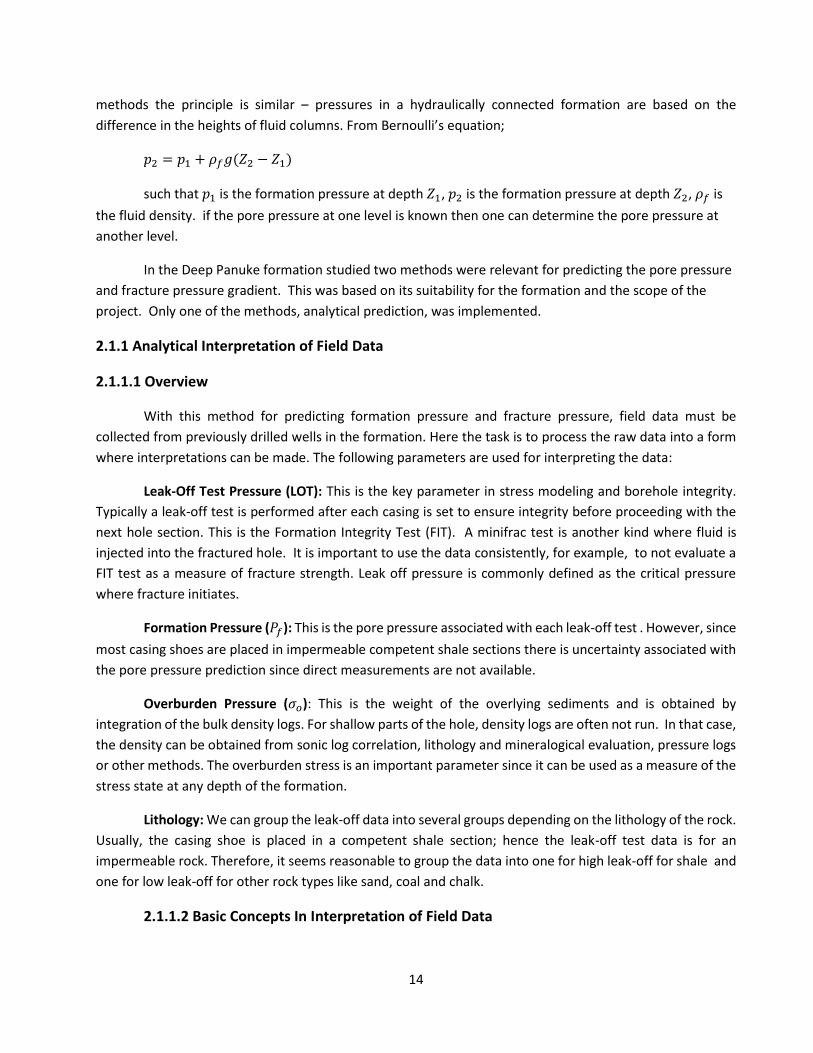
methods the principle is similar – pressures in a hydraulically connected formation are based on the

difference in the heights of fluid columns. From Bernoulli’s equation;

𝑝2 = 𝑝1 + 𝜌𝑓𝑔(𝑍2 − 𝑍1)

such that 𝑝1 is the formation pressure at depth 𝑍1, 𝑝2 is the formation pressure at depth 𝑍2, 𝜌𝑓 is

the fluid density. if the pore pressure at one level is known then one can determine the pore pressure at

another level.

In the Deep Panuke formation studied two methods were relevant for predicting the pore pressure

and fracture pressure gradient. This was based on its suitability for the formation and the scope of the

project. Only one of the methods, analytical prediction, was implemented.

2.1.1 Analytical Interpretation of Field Data

2.1.1.1 Overview

With this method for predicting formation pressure and fracture pressure, field data must be

collected from previously drilled wells in the formation. Here the task is to process the raw data into a form

where interpretations can be made. The following parameters are used for interpreting the data:

Leak-Off Test Pressure (LOT): This is the key parameter in stress modeling and borehole integrity.

Typically a leak-off test is performed after each casing is set to ensure integrity before proceeding with the

next hole section. This is the Formation Integrity Test (FIT). A minifrac test is another kind where fluid is

injected into the fractured hole. It is important to use the data consistently, for example, to not evaluate a

FIT test as a measure of fracture strength. Leak off pressure is commonly defined as the critical pressure

where fracture initiates.

Formation Pressure (𝑃𝑓): This is the pore pressure associated with each leak-off test . However, since

most casing shoes are placed in impermeable competent shale sections there is uncertainty associated with

the pore pressure prediction since direct measurements are not available.

Overburden Pressure (𝜎𝑜): This is the weight of the overlying sediments and is obtained by

integration of the bulk density logs. For shallow parts of the hole, density logs are often not run. In that case,

the density can be obtained from sonic log correlation, lithology and mineralogical evaluation, pressure logs

or other methods. The overburden stress is an important parameter since it can be used as a measure of the

stress state at any depth of the formation.

Lithology: We can group the leak-off data into several groups depending on the lithology of the rock.

Usually, the casing shoe is placed in a competent shale section; hence the leak-off test data is for an

impermeable rock. Therefore, it seems reasonable to group the data into one for high leak-off for shale and

one for low leak-off for other rock types like sand, coal and chalk.

2.1.1.2 Basic Concepts In Interpretation of Field Data

15

Process

This involves performing a field analysis then data collection. The modelling procedure is to first

normalize the data for known factors – drill floor elevation, water depth or other differences. Secondly, if

the data set consists of data from vertical and inclined borehole, they could be grouped accordingly. Thirdly,

if there are known differences in lithology, the data should preferably be divided between the two groups

defined above. Once the data set is consistent then model them.

Evaluate Leak-off data

The leak-off test data often shows considerable spread. From evaluating only this single parameter in

isolation it is difficult to obtain good correlations. However, as a starting point for the analysis, one should

start with a plot of the LOT data versus depth. Remember the quality of the analysis results mainly from

demonstrating an improved degree of correlation when additional factors are considered.

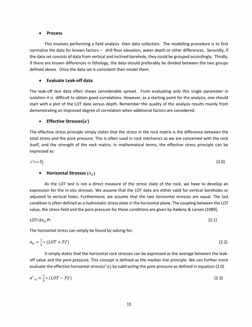
Effective Stresses(s')

The effective stress principle simply states that the stress in the rock matrix is the difference between the

total stress and the pore pressure. This is often used in rock mechanics as we are concerned with the rock

itself, and the strength of the rock matrix. In mathematical terms, the effective stress principle can be

expressed as:

s'=s-𝑃𝑓 (2.0)

Horizontal Stresses(𝜎𝑎)

As the LOT test is not a direct measure of the stress state of the rock, we have to develop an

expression for the in-situ stresses. We assume that the LOT data are either valid for vertical boreholes or

adjusted to vertical holes. Furthermore; we assume that the two horizontal stresses are equal. The last

condition is often defined as a hydrostatic stress state in the horizontal plane. The coupling between the LOT

value, the stress field and the pore pressure for these conditions are given by Aadony & Larsen (1989),

LOT=2𝜎𝑎-Pf (2.1)

The horizontal stress can simply be found by solving for:

𝜎𝑎 =1

2∗ (𝐿𝑂𝑇 + 𝑃𝑓) (2.2)

It simply states that the horizontal rock stresses can be expressed as the average between the leak-

off value and the pore pressure. This concept is defined as the median line principle. We can further more

evaluate the effective horizontal stress(𝜎′𝑎) by subtracting the pore pressure as defined in equation (2.0)

𝜎′ 𝑎 =1

2∗ (𝐿𝑂𝑇 − 𝑃𝑓) (2.3)

16

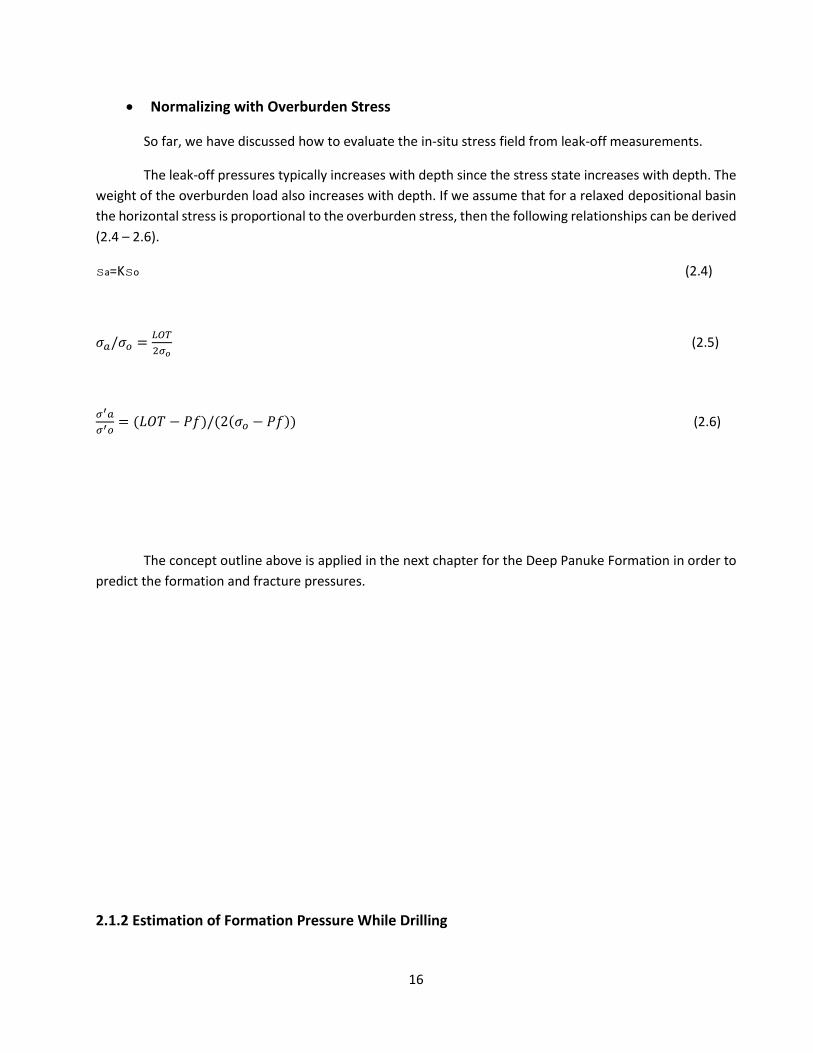
Normalizing with Overburden Stress

So far, we have discussed how to evaluate the in-situ stress field from leak-off measurements.

The leak-off pressures typically increases with depth since the stress state increases with depth. The

weight of the overburden load also increases with depth. If we assume that for a relaxed depositional basin

the horizontal stress is proportional to the overburden stress, then the following relationships can be derived

(2.4 – 2.6).

sa=Kso (2.4)

𝜎𝑎/𝜎𝑜 =𝐿𝑂𝑇

2𝜎𝑜 (2.5)

𝜎′𝑎

𝜎′𝑜= (𝐿𝑂𝑇 − 𝑃𝑓)/(2(𝜎𝑜 − 𝑃𝑓)) (2.6)

The concept outline above is applied in the next chapter for the Deep Panuke Formation in order to

predict the formation and fracture pressures.

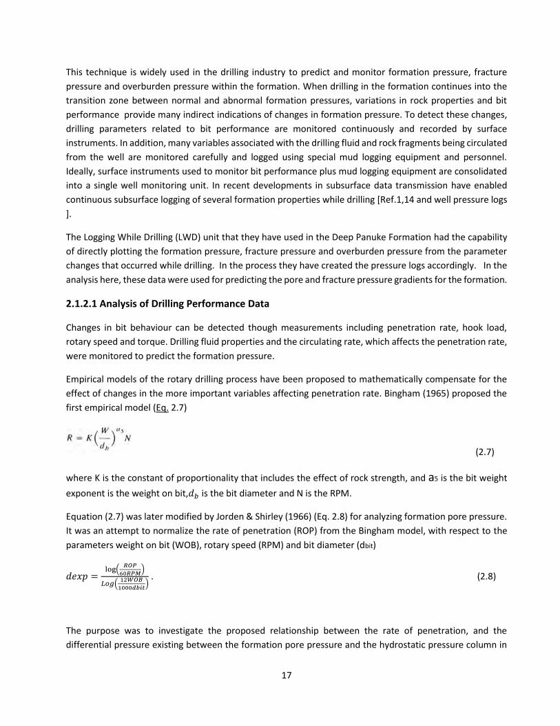
2.1.2 Estimation of Formation Pressure While Drilling

17

This technique is widely used in the drilling industry to predict and monitor formation pressure, fracture

pressure and overburden pressure within the formation. When drilling in the formation continues into the

transition zone between normal and abnormal formation pressures, variations in rock properties and bit

performance provide many indirect indications of changes in formation pressure. To detect these changes,

drilling parameters related to bit performance are monitored continuously and recorded by surface

instruments. In addition, many variables associated with the drilling fluid and rock fragments being circulated

from the well are monitored carefully and logged using special mud logging equipment and personnel.

Ideally, surface instruments used to monitor bit performance plus mud logging equipment are consolidated

into a single well monitoring unit. In recent developments in subsurface data transmission have enabled

continuous subsurface logging of several formation properties while drilling [Ref.1,14 and well pressure logs

].

The Logging While Drilling (LWD) unit that they have used in the Deep Panuke Formation had the capability

of directly plotting the formation pressure, fracture pressure and overburden pressure from the parameter

changes that occurred while drilling. In the process they have created the pressure logs accordingly. In the

analysis here, these data were used for predicting the pore and fracture pressure gradients for the formation.

2.1.2.1 Analysis of Drilling Performance Data

Changes in bit behaviour can be detected though measurements including penetration rate, hook load,

rotary speed and torque. Drilling fluid properties and the circulating rate, which affects the penetration rate,

were monitored to predict the formation pressure.

Empirical models of the rotary drilling process have been proposed to mathematically compensate for the

effect of changes in the more important variables affecting penetration rate. Bingham (1965) proposed the

first empirical model (Eq. 2.7)

(2.7)

where K is the constant of proportionality that includes the effect of rock strength, and a5 is the bit weight

exponent is the weight on bit,𝑑𝑏 is the bit diameter and N is the RPM.

Equation (2.7) was later modified by Jorden & Shirley (1966) (Eq. 2.8) for analyzing formation pore pressure.

It was an attempt to normalize the rate of penetration (ROP) from the Bingham model, with respect to the

parameters weight on bit (WOB), rotary speed (RPM) and bit diameter (dbit)

𝑑𝑒𝑥𝑝 =log(

𝑅𝑂𝑃

60𝑅𝑃𝑀)

𝐿𝑜𝑔(12𝑊𝑂𝐵

1000𝑑𝑏𝑖𝑡) . (2.8)

The purpose was to investigate the proposed relationship between the rate of penetration, and the

differential pressure existing between the formation pore pressure and the hydrostatic pressure column in

18

the wellbore. Knowledge of this relationship would make it possible to predict changes in the pore pressure

with respect to the obtained drilling data.

The d-exponent method (Eq. 2.8) can be utilized to identify transition zones going from a normal pressurized

zone into an abnormal pressurized zone. This can be done by acquiring data from formations assumed to

have a normal pressure gradient and creating a plot between d-exponent and the vertical depth. For a

normally pressurized formation d-exponent shows an increase as the depth increases. When it encounters

an abnormally pressured formation d-exponent starts to diminish. in some cases reverse trends with depth

are observed.

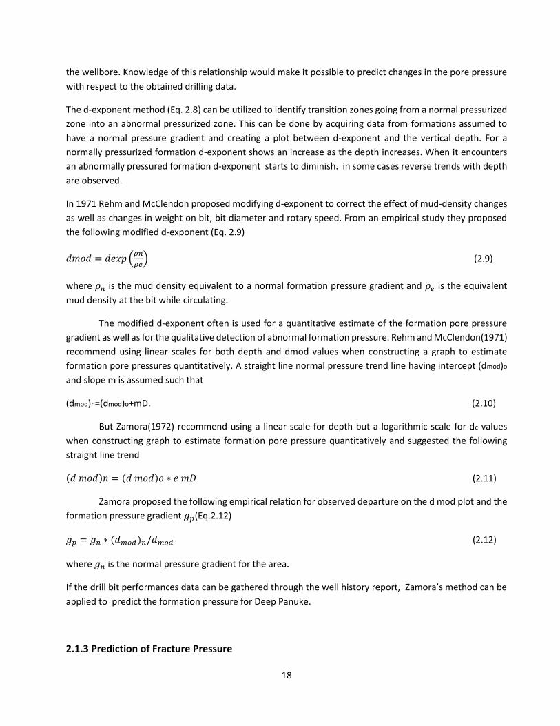
In 1971 Rehm and McClendon proposed modifying d-exponent to correct the effect of mud-density changes

as well as changes in weight on bit, bit diameter and rotary speed. From an empirical study they proposed

the following modified d-exponent (Eq. 2.9)

𝑑𝑚𝑜𝑑 = 𝑑𝑒𝑥𝑝 (𝜌𝑛

𝜌𝑒) (2.9)

where 𝜌𝑛 is the mud density equivalent to a normal formation pressure gradient and 𝜌𝑒 is the equivalent

mud density at the bit while circulating.

The modified d-exponent often is used for a quantitative estimate of the formation pore pressure

gradient as well as for the qualitative detection of abnormal formation pressure. Rehm and McClendon(1971)

recommend using linear scales for both depth and dmod values when constructing a graph to estimate

formation pore pressures quantitatively. A straight line normal pressure trend line having intercept (dmod)o

and slope m is assumed such that

(dmod)n=(dmod)o+mD. (2.10)

But Zamora(1972) recommend using a linear scale for depth but a logarithmic scale for dc values

when constructing graph to estimate formation pore pressure quantitatively and suggested the following

straight line trend

(𝑑 𝑚𝑜𝑑)𝑛 = (𝑑 𝑚𝑜𝑑)𝑜 ∗ 𝑒 𝑚𝐷 (2.11)

Zamora proposed the following empirical relation for observed departure on the d mod plot and the

formation pressure gradient 𝑔𝑝(Eq.2.12)

𝑔𝑝 = 𝑔𝑛 ∗ (𝑑𝑚𝑜𝑑)𝑛/𝑑𝑚𝑜𝑑 (2.12)

where 𝑔𝑛 is the normal pressure gradient for the area.

If the drill bit performances data can be gathered through the well history report, Zamora’s method can be

applied to predict the formation pressure for Deep Panuke.

2.1.3 Prediction of Fracture Pressure

19

Fracture pressure is the pressure required to fracture the formation and cause mud loss from the

wellbore into the induced fracture. Normally, the fracture gradient can obtain by dividing out the true vertical

depth from the fracture pressure. In other words it is the maximum mud weight that can be used to drill a

well bore at a given depth. Hence it is an important parameter for mud weight design in both the drilling

planning stage and while drilling. If the mud weight is higher than the fracture gradient of the formation the

well bore will undergo tensile failure, causing losses of drilling mud or even lost circulation. In practice

fracture pressure is measured from leak-off tests (LOT). There are several approaches to calculate fracture

gradient. From the literature review the most widely used is the Ben Eaton fracture gradient prediction

strategy [1975].

In 1996, Yoshida et al published results of a study that analysed the currently used technologies used

to predict, detect and evaluate the abnormal pressure and fracture pressure gradients in formations all over

the world. This study revealed Ben Eaton’s fracture gradient prediction strategy is one of the best methods

to apply.

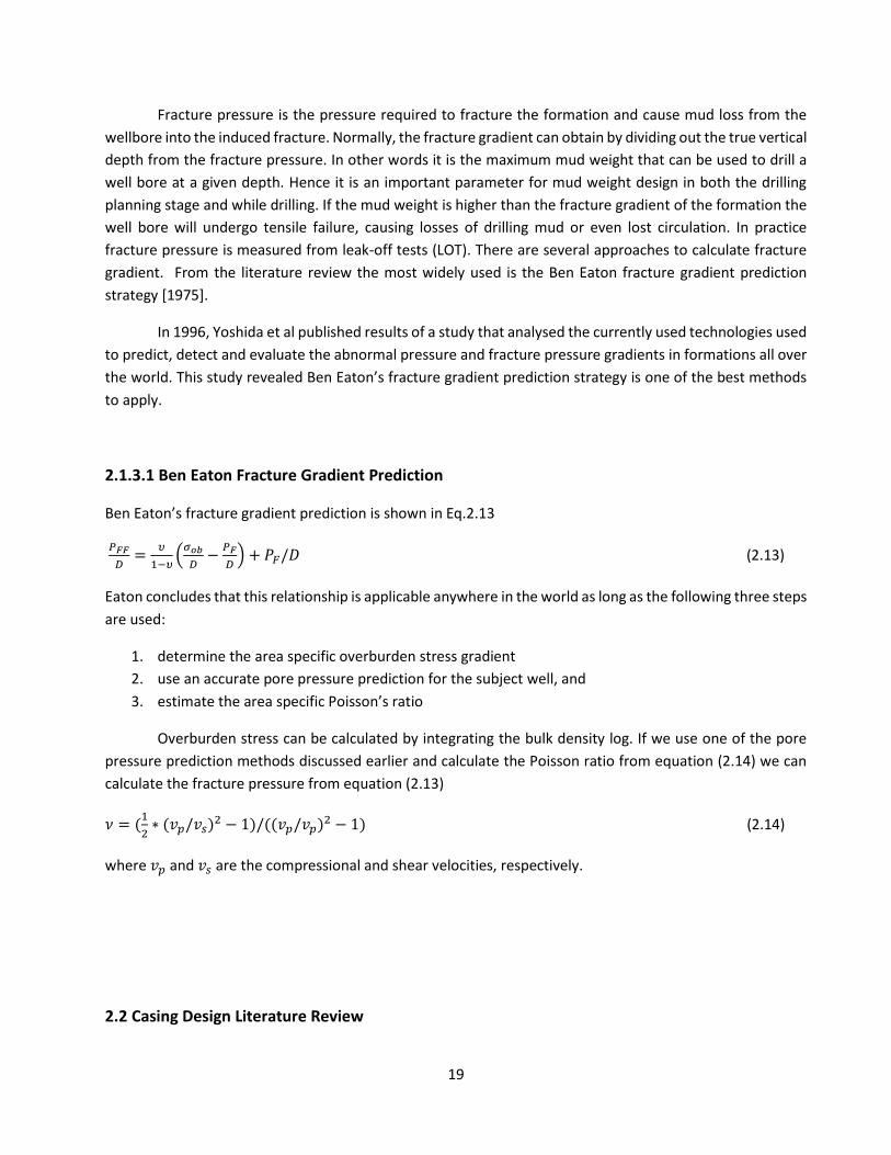
2.1.3.1 Ben Eaton Fracture Gradient Prediction

Ben Eaton’s fracture gradient prediction is shown in Eq.2.13

𝑃𝐹𝐹

𝐷=

𝜐

1−𝜐(

𝜎𝑜𝑏

𝐷−

𝑃𝐹

𝐷) + 𝑃𝐹/𝐷 (2.13)

Eaton concludes that this relationship is applicable anywhere in the world as long as the following three steps

are used:

1. determine the area specific overburden stress gradient

2. use an accurate pore pressure prediction for the subject well, and

3. estimate the area specific Poisson’s ratio

Overburden stress can be calculated by integrating the bulk density log. If we use one of the pore

pressure prediction methods discussed earlier and calculate the Poisson ratio from equation (2.14) we can

calculate the fracture pressure from equation (2.13)

𝜈 = (1

2∗ (𝑣𝑝/𝑣𝑠)2 − 1)/((𝑣𝑝/𝑣𝑝)2 − 1) (2.14)

where 𝑣𝑝 and 𝑣𝑠 are the compressional and shear velocities, respectively.

2.2 Casing Design Literature Review

20

2.2.1Introduction

A casing is a large heavy steel pipe which can be lowered into the well, Generally a casing is subjected

to various physical and chemically related loads during its life time. Its purpose is to prevent collapse of the

borehole while drilling, hydraulically isolate the wellbore fluids from formations and formation fluid,

minimize damage of both the subsurface environment from the drilling process and from extreme subsurface

environment, provide a high strength flow conduit for the drilling fluid, provide safe control of formation

pressure, and if the casing is properly cemented it can help to isolate communications between different

perforated formation levels. In selection of the number of casing string and their respective setting depths

generally is based on a consideration of the pore-pressure gradients and fracture gradients of the area that

the drilling is going to perform.

21

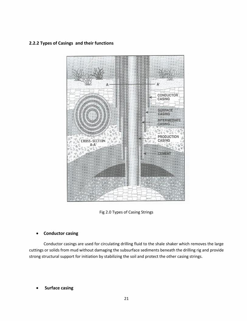
2.2.2 Types of Casings and their functions

Fig 2.0 Types of Casing Strings

Conductor casing

Conductor casings are used for circulating drilling fluid to the shale shaker which removes the large

cuttings or solids from mud without damaging the subsurface sediments beneath the drilling rig and provide

strong structural support for initiation by stabilizing the soil and protect the other casing strings.

Surface casing

22

The main purpose of the surface casing is to protect the shallow water region from contamination,

give structural support for weak soil areas near the subsurface, and also protect the casing strings inside.

Again, this can prevent blow-out and can close the surface casing in the event of a kick or explosion.

Intermediate casing

When drilling deeper through weak zones like salt sections and abnormally pressurized formations

these unstable sections need more pipe sections, in the form of intermediate casings, between the surface

casing and the final casing. When abnormal pore pressures are present below the surface casing

intermediate casings are needed to protect the formation.

Liners

The liner is a casing string that does not extend to the surface. It is suspended from the bottom of

the next large casing string. The principal advantage of a liner is its lower cost. It serves as a low cost

intermediate casing.

Production Casing

This casing string provides protection for the environment in the event of a failure during production.

Production casings are connected to wellhead using a tie-back when the well is completed. This casing is

used for the entire interval of the drilling.

2.2.3 Design Criteria

Casing strings have different functions as explained above. The conductor casing has the role of

supporting the well head. With the exception of the production case, the casing strings have temporary

functions. During the life time of the well production the casing’s structural integrity cannot be

compromised.

One of the most critical activities in designing a well is the selection of the casing design criteria. The

casing design involves a strength assessment for burst, collapse and tensional loads on the casing string.

When the surface casing was designed for the proposed Deep Panuke development well, failure scenarios

for: collapse, burst , tension, biaxial loading, temperatures, long time intervals, casing wear, field handling

effects, casing landing effect, internal pressure variations, sour service (effect of hydrogen sulfide) and shock

failure were evaluated and considered.

2.2.3.1 Burst Mechanism

The pipe body will have a tendency to burst when the differences between the internal and external

pressures exceeds the mechanical strength of the pipe. Burst is a tensile failure resulting in rupture along the

axis of the pipe. From the design point of view the following categories is considered

1. Gas filled Casing

23

It is assumed the well is completely filled with gas or formation fluids and then shut in. When

this happens the inside pressure below the wellhead will be the formation pressures minus the

weight of the gas column. The outside pressure on the casing is usually the hydrostatic weight of the

fluids behind the casing string. The gas filled casing scenario should be applied to the production

casing because, when the well is tested and produced, there is a potential exposure to gas filled

casing.

2. Leaking tubing criterion

During well testing or production, leaks can occur at the top of the production tubing just

below the wellhead. If a leak occurs at the top of the tubing the inside tubing pressure is

superimposed on top of the casing/tubing annulus. Therefore, due to the combined hydrostatic head

a significant pressure can build in the casing annulus (space between casing and drill pipe).

3. Maximum Gas Kick

This is based on the largest gas influx volume which can enter the wellbore at the next casing

setting depth (end of next casing level) and be circulated out without fracturing the formation at the

previous casing shoe.

2.2.3.2 Collapse Mechanisms

When a casing collapses due to external loading it changes its shape from circular to elliptical or some other

non-circular shape. The casing will collapse when the external pressure acting on the casing body exceeds

the internal pressure. Collapse is a deformation of the casing and geometric failure rather than a material

failure.

According to the API Bulletin 5C3, (1990), the collapse pressure is given by Eq. (2.15)

𝑃𝑐𝑜𝑙𝑙𝑎𝑝𝑠𝑒 =2𝐶𝐸

1−𝜈2 ∗ {1

𝐷𝑜𝑡

−1)2𝐷𝑜

𝑡

} . (2.15)

It is observed that casing wear can considerably impact on the collapse resistance. In collapse design the

following categories are considered

1. Mud loss to thief zone

During drilling mud losses can occur unexpectedly. When this happens the fluid level in the

annulus (space between drill pipe and casing) can drop. When mud is lost the pressure outside the casing

remains constant. But the inside pressure decreases creating a condition that makes the casing

vulnerable to collapse.

2. Collapse during cementing

In drilling operations cement is used to protect and support the casings, prevent the movement of

fluid through annular space (between the outside the casing and borehole) and stop movement of fluid into

fractured formations. Immediately after cementing there is a hydrostatic wet cement pressure along the

whole surface casing. Due to this there will be a pressure difference that could build towards a collapse

pressure.

24

2.2.3.3 Tension Mechanism

Tension failure occurs when the axial loads exceed the material strength resulting in a parted pipe

or connection. The maximum load during installation of a casing string should be evaluated. This must also

take into account drag forces if the casing will temporarily be pulled. When designing for tension the

following forces must be considered

1. Weight in air minus buoyancy force, plus bending forces, plus drag forces, plus load from pressure

testing or

2. Weight in air minus buoyancy force, plus bending force, plus drag force, plus shock load. (to check

these tensile failure checks needs to be carried out as per API standards)

2.2.3.4 Temperature effects

The strength of the casing decreases as the temperature increases. In a deeper high pressure well

the temperature margins for strength are often small, and temperature strength reduction is called for.

Another problem caused by temperature change is pressure build up in closed annuli.

2.2.3.5 Biaxial Loading

There are three main stresses acting on the casing string the axial, radial and tangential or hoop load. All

these forces are simultaneously present to some extent on the string. Here, coupled loading conditions are

analysed. The tensional strength depends on the axial tension while both the burst and collapse are

functions of the hoop stress. This means hoop and axial stresses govern all the failure mechanisms. The

radial stress is a loading factor but no radial failure mechanism has been addressed. Therefore from a

failure point of view we can neglect radial failure as it has a little effect. The biaxial failure mode can be

defined by the following equation

𝜎𝑡

𝜎𝑦𝑖𝑒𝑙𝑑=

1

2∗ 𝜎𝑑/𝜎𝑦𝑖𝑒𝑙𝑑 ± √(1 −

3

4∗ (𝜎𝑎/𝜎𝑦𝑖𝑒𝑙𝑑)2) (2.16)

Eq. (2.16) shows the reduction in collapse strength as a function of axial tension. It must be emphasised that

in casing design practice, the ellipse of plasticity cannot be applied unless the assumption of a yield strength

mode of failure is known to be valid (Bent S.Aadnoy, Modern Well Design 2010). If a very high material grade

casing is used the string may fail in a brittle manner before significant yield occurs.

25

2.2.3.6 Sour Service

This considers the effect of corrosive gases in the borehole. For this two aspects are considered.

1. Corrosion that leads to long term material failure, and

2. Hydrogen embrittlement that may lead to failure on a short term basis.

If corrosive elements are expected typically the bottom part of the production casing is made of a

quality stainless steel and often with an increased wall thickness as a corrosion allowance. There are no

simple methods to design the production casing for corrosive environments. In this case judgement and

experience often form the basis for material selection.

2.2.3.7 Time Scenario

Generally there are two types of wells. The first are exploration wells that are drilled and abandoned

within a few months. The second are production wells that are used continuously through their life. So when

designing wells the time is a factor that should be addressed when selecting materials.

2.2.3.7 Casing Wear

Casing wear may become important if it reduces its burst resistance. It is difficult to predict wear

but it is often related to the number of hours the drilling string is being rotated inside the casing.

2.2.3.8 Casing Landing effect

In some cases when the casing is landed, considerable additional axial stress will be placed in the casing at

the well head.API committee identified the following four common methods for landing casing.

1. Landing the casing with the same tension that was present when cement displacement was

completed.

2. Landing the casing in tension at the freeze point, this is generally considered to be at the top of

the cement.

3. Landing the casing with the neutral point of axial stress at the freeze point.

4. Landing the casing in compression at the freeze point.

Though all the general procedures are still used within the industry,API has recently withdrawn Bulletin D-

7,hence it currently does not have a recommended casing landing practice.( Adam T.Bourgene Jr., Keith

K.Milleim, Martin E.Chenvert, and F.S.Young Jr.(1986).)

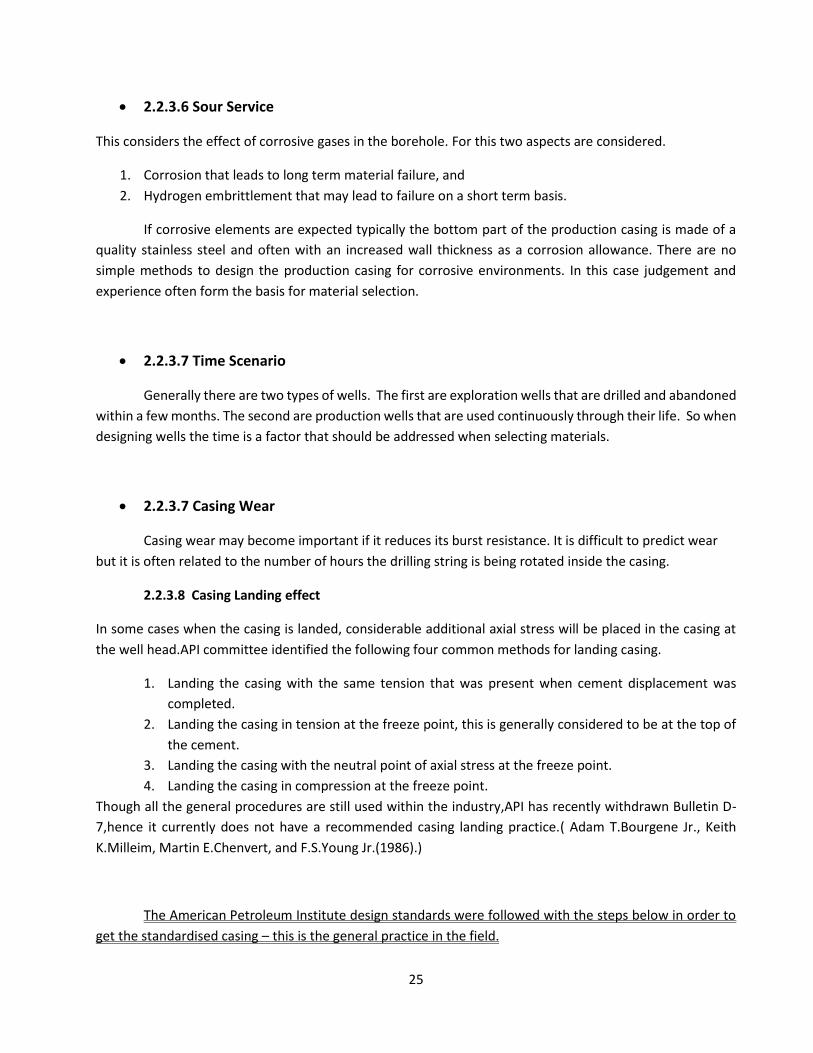
The American Petroleum Institute design standards were followed with the steps below in order to

get the standardised casing – this is the general practice in the field.

26

1. Get the pore pressure and fracture pressure chart finalized from the first part of the project

2. Select the casing setting depths

3. Select the Casing sizes

4. Determine the number of casing required

5. Perform design calculations and select the casing tubing grades and couplings

Fig 2.1 Pore pressure and fracture pressure model-Deep Panuke formation

3. Deep Panuke Offset Well Data Review

One of the main strategies in practice for developing an accurate pore and fracture pressure

gradient prediction is to analyse the offset well data in the formation of interest. Here, all the pressure

0

500

1000

1500

2000

2500

3000

3500

4000

0 500 1000 1500 2000

Ve

rtic

al D

ep

th m

Pressure Gradient Kg/m³

Pore and Fracture Pressure Design Lines for New Well

Pore Pressure Design Line ForNW

Fracture Pressure Design LineFor NW

Design Pore Pressure Line

Design Fracture Pressure Line

27

related data available for the Deep Panuke gas pool from well history reports, logs and other studies were

reviewed. This includes mud weight, kicks, leaks-off tests, lost circulations, formation pressures measured

from well tests and pressure data taken from the well pressure logs. Again, the objective is pore pressure

and fracture pressure predictions, in the form of a model, for the Deep Panuke gas pool.(data in Apendix-1)

3.1 Drilling Data Review

Here the data being analysed was obtained from the well history reports, mud logs, and pressure

logs available at the Canada Nova Scotia Offshore Petroleum Board (CNSOPB) research center.

One of the main important pieces of drilling data available is the actual drilling mud weight versus

the depth relationship for each well in the pool. These mud weights relative to the depth can be taken from

daily summary report, well logs or history report. This is very useful for representing the maximum expected

value for pore pressure since the drilling mud weights, in these cases, apply sufficient hydrostatic pressure

to control formation pressures in areas of permeable zones.

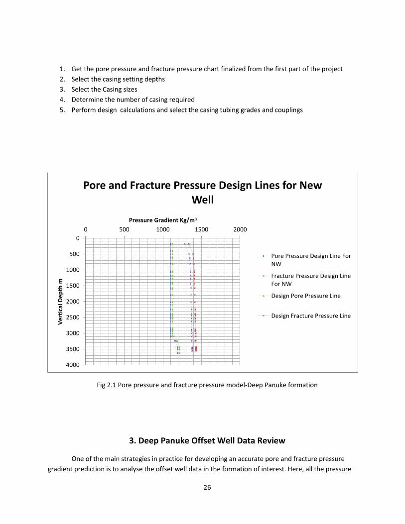
All the drilling mud data obtained from each well in the pool is tabulated in the Apendix-1 (all the

references which the data have been picked is listed in each table). Fig. 3.1 is a graph of the vertical depth

versus the actual drilling mud density.

Fig.3.1 Vertical depth versus actual drilling mud density

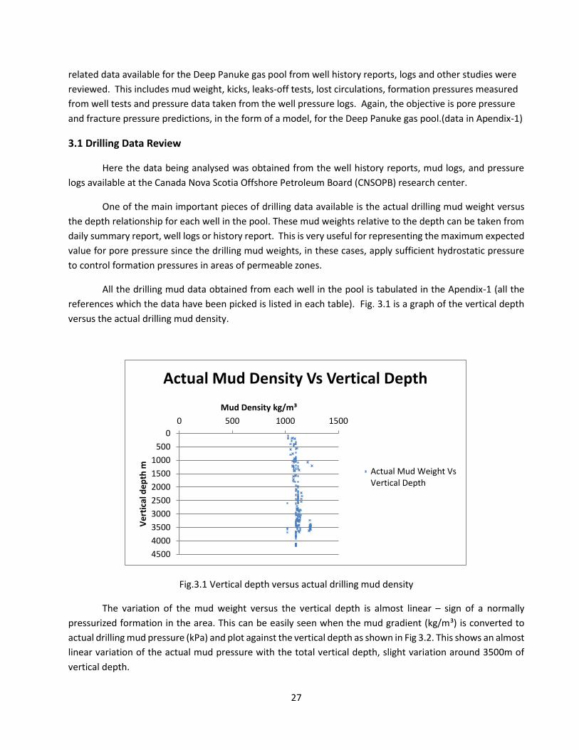
The variation of the mud weight versus the vertical depth is almost linear – sign of a normally

pressurized formation in the area. This can be easily seen when the mud gradient (kg/m³) is converted to

actual drilling mud pressure (kPa) and plot against the vertical depth as shown in Fig 3.2. This shows an almost

linear variation of the actual mud pressure with the total vertical depth, slight variation around 3500m of

vertical depth.

0

500

1000

1500

2000

2500

3000

3500

4000

4500

0 500 1000 1500

Ve

rtic

al d

ep

th m

Mud Density kg/m³

Actual Mud Density Vs Vertical Depth

Actual Mud Weight VsVertical Depth

28

Fig 3.2 Actual drilling mud pressure versus vertical depth

Normally, when a well is drilled and cased, leak-off tests (LOTs) are performed after the first casing

to determine the real-time fracture gradients before the next section is drilled. This gives an indication of

maximum mud weight that can be used below this section. Table 3.1 summarizes the LOTs data from the

Deep Panuke gas pool.

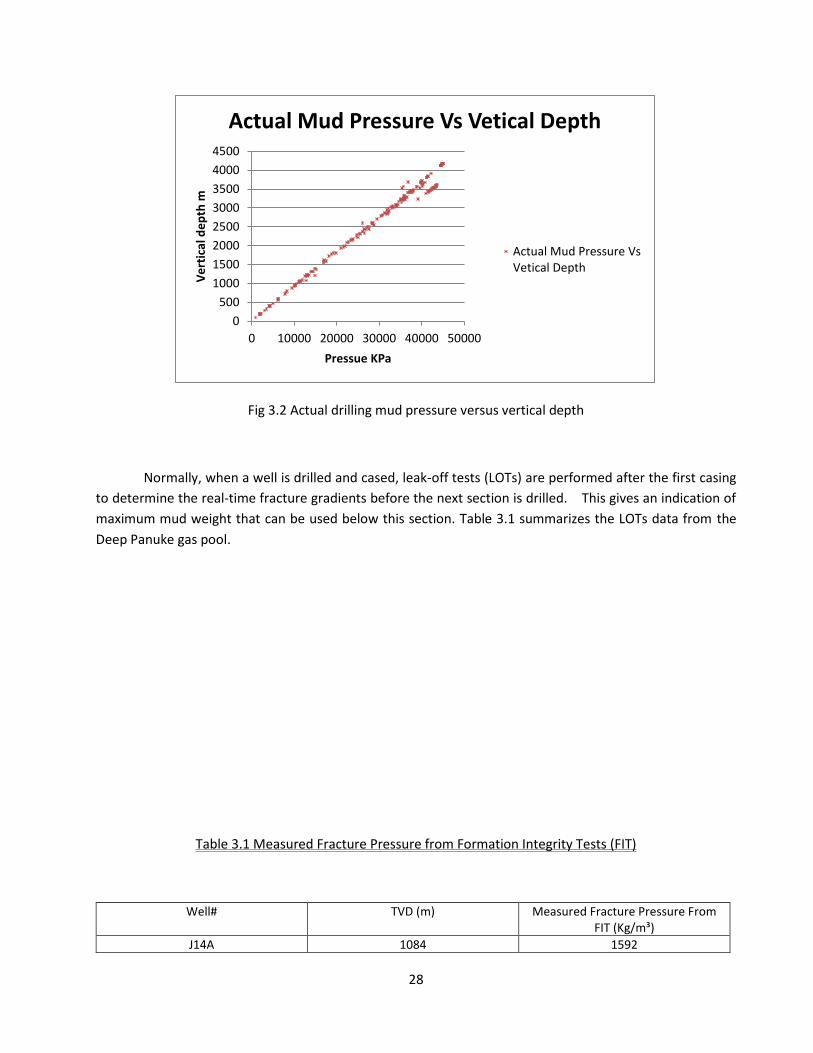
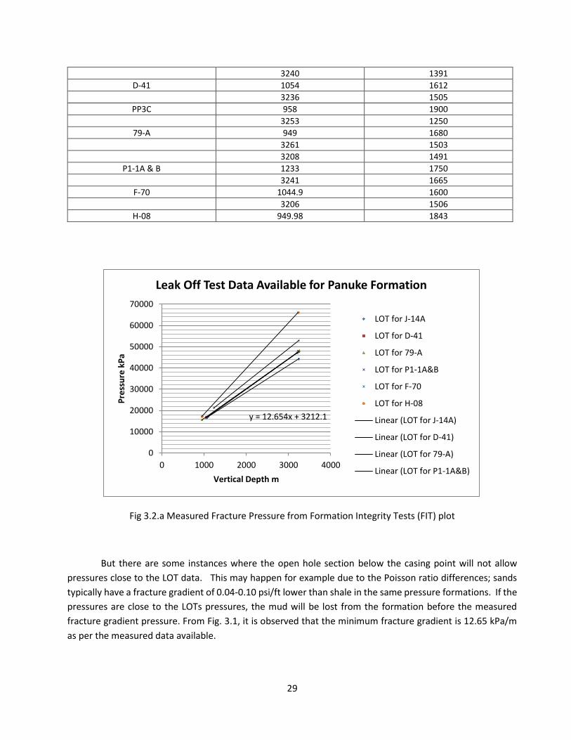
Table 3.1 Measured Fracture Pressure from Formation Integrity Tests (FIT)

Well# TVD (m) Measured Fracture Pressure From FIT (Kg/m³)

J14A 1084 1592

0

500

1000

1500

2000

2500

3000

3500

4000

4500

0 10000 20000 30000 40000 50000

Ve

rtic

al d

ep

th m

Pressue KPa

Actual Mud Pressure Vs Vetical Depth

Actual Mud Pressure VsVetical Depth

29

3240 1391

D-41 1054 1612

3236 1505

PP3C 958 1900

3253 1250

79-A 949 1680

3261 1503

3208 1491

P1-1A & B 1233 1750

3241 1665

F-70 1044.9 1600

3206 1506

H-08 949.98 1843

Fig 3.2.a Measured Fracture Pressure from Formation Integrity Tests (FIT) plot

But there are some instances where the open hole section below the casing point will not allow

pressures close to the LOT data. This may happen for example due to the Poisson ratio differences; sands

typically have a fracture gradient of 0.04-0.10 psi/ft lower than shale in the same pressure formations. If the

pressures are close to the LOTs pressures, the mud will be lost from the formation before the measured

fracture gradient pressure. From Fig. 3.1, it is observed that the minimum fracture gradient is 12.65 kPa/m

as per the measured data available.

y = 12.654x + 3212.1

0

10000

20000

30000

40000

50000

60000

70000

0 1000 2000 3000 4000

Pre

ssu

re k

Pa

Vertical Depth m

Leak Off Test Data Available for Panuke Formation

LOT for J-14A

LOT for D-41

LOT for 79-A

LOT for P1-1A&B

LOT for F-70

LOT for H-08

Linear (LOT for J-14A)

Linear (LOT for D-41)

Linear (LOT for 79-A)

Linear (LOT for P1-1A&B)

30

Another important source of information is the drilling incidents faced in the local area. Well control

events such as kicks and lost circulation events are a good indication of the minimum and maximum pressures

allowed during the drilling operations. These data can be used to predict an accurate pore and fracture

pressure gradient. Table 3.2 summarizes the drilling pressure related problems encountered in the Deep

Panuke Pool.

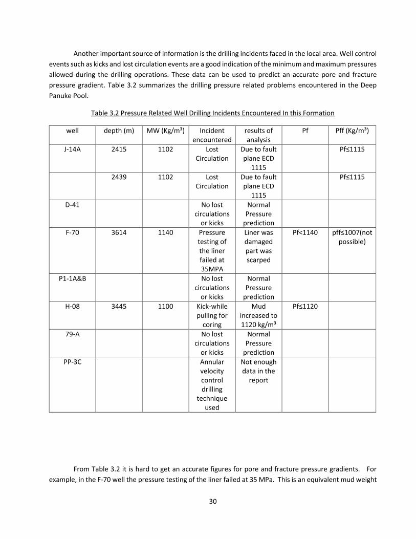
Table 3.2 Pressure Related Well Drilling Incidents Encountered In this Formation

well depth (m) MW (Kg/m³) Incident encountered

results of analysis

Pf Pff (Kg/m³)

J-14A 2415 1102 Lost Circulation

Due to fault plane ECD

1115

Pf≤1115

2439 1102 Lost Circulation

Due to fault plane ECD

1115

Pf≤1115

D-41 No lost circulations

or kicks

Normal Pressure

prediction

F-70 3614 1140 Pressure testing of the liner failed at 35MPA

Liner was damaged part was scarped

Pf<1140 pff≤1007(not possible)

P1-1A&B No lost circulations

or kicks

Normal Pressure

prediction

H-08 3445 1100 Kick-while pulling for

coring

Mud increased to 1120 kg/m³

Pf≤1120

79-A No lost circulations

or kicks

Normal Pressure

prediction

PP-3C Annular velocity control drilling

technique used

Not enough data in the

report

From Table 3.2 it is hard to get an accurate figures for pore and fracture pressure gradients. For

example, in the F-70 well the pressure testing of the liner failed at 35 MPa. This is an equivalent mud weight

31

of 1007 kg/m³. But that liner could hold 1140kg/m³ mud weight before testing which means the pore

pressure at that depth is greater than 1140Kg/m³. However, the recorded 35MPa pressure does not interpret

the fracture pressure information. In other words, to get the correct fracture pressure the failure pressure

cannot be used. Most of Table 3.2 is weak in determining the pore and fracture gradients. They can still be

used as reference values when predicting the final pore and fracture pressure model for the formation.

3.2 Measured Pressure Data Analysis

In the Deep Panuke gas pool there are two wells where they have carried out either the Repeat

Formation Test (RFT) or Modular Dynamics Test (MDT) to determine the reservoir formation pressures and

hydrostatic pressures. These tests are expensive and rarely carried out but they give very accurate results

(unless the tool malfunctions or there is no good formation permeability with which to provide accurate

measurements). These data are used to validate the pore pressure prediction methods used.

From the test tools data categories like “dry test”, “limited drawdown”, “lost seal” or “super charge“

were erroneous so they are ignored. Data categories of “normal pre-test”, “Good Test” or “Repeat Test” are

retained for the analysis here. Furthermore, measurements of the hydrostatic pressure prior to and after a

pressure measurement are available and useful for this analysis.

MDT & RFT data obtained for the Deep Panuke pool tabulated in Appendix-2. Fig.3.3 and Fig.3.4

shows plots of measured reservoir formation pressures and hydrostatic pressure exerted by the drilling mud

for the two offset wells D-41 & 79A. These were plotted using the validated data from the Table1 and Table2

in Appendix-2.

3350.00

3400.00

3450.00

3500.00

3550.00

3600.00

30000 32000 34000 36000 38000 40000 42000 44000 46000

Ve

tica

l De

pth

m

Pressure kPa

Measured Formation Pressure Vs Vertical Depth For Well # D41

Formation Pressure

Hydrostatic Pressure

32

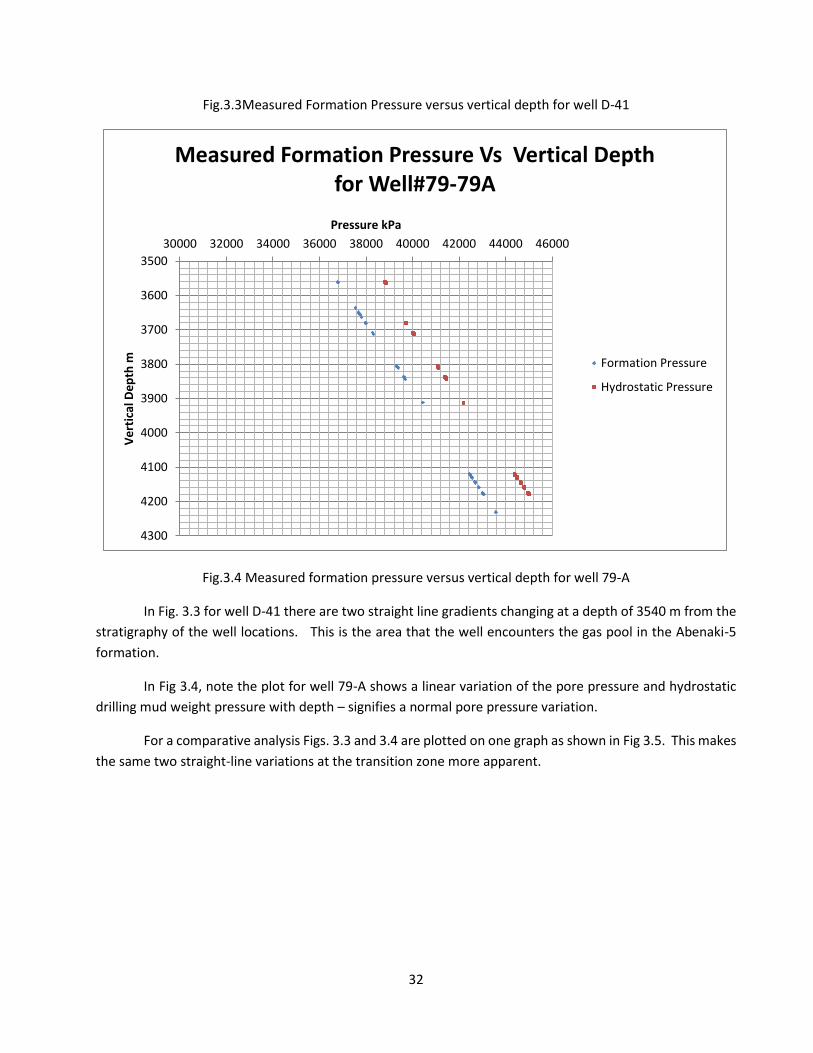
Fig.3.3Measured Formation Pressure versus vertical depth for well D-41

Fig.3.4 Measured formation pressure versus vertical depth for well 79-A

In Fig. 3.3 for well D-41 there are two straight line gradients changing at a depth of 3540 m from the

stratigraphy of the well locations. This is the area that the well encounters the gas pool in the Abenaki-5

formation.

In Fig 3.4, note the plot for well 79-A shows a linear variation of the pore pressure and hydrostatic

drilling mud weight pressure with depth – signifies a normal pore pressure variation.

For a comparative analysis Figs. 3.3 and 3.4 are plotted on one graph as shown in Fig 3.5. This makes

the same two straight-line variations at the transition zone more apparent.

3500

3600

3700

3800

3900

4000

4100

4200

4300

30000 32000 34000 36000 38000 40000 42000 44000 46000

Ve

rtic

al D

ep

th m

Pressure kPa

Measured Formation Pressure Vs Vertical Depth for Well#79-79A

Formation Pressure

Hydrostatic Pressure

33

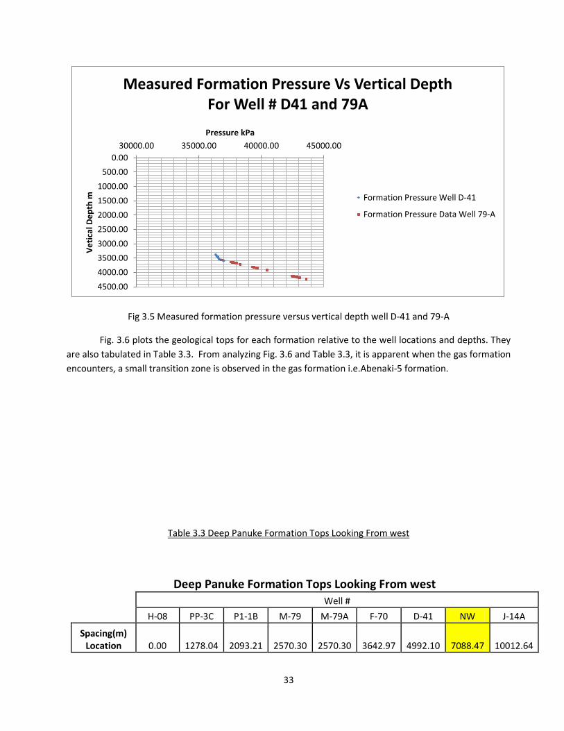
Fig 3.5 Measured formation pressure versus vertical depth well D-41 and 79-A

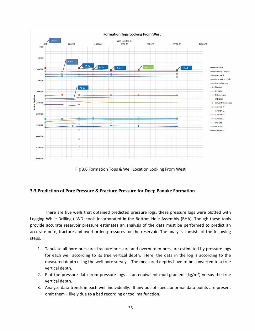
Fig. 3.6 plots the geological tops for each formation relative to the well locations and depths. They

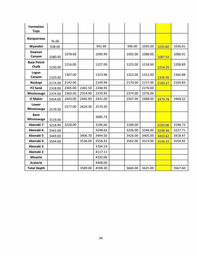
are also tabulated in Table 3.3. From analyzing Fig. 3.6 and Table 3.3, it is apparent when the gas formation

encounters, a small transition zone is observed in the gas formation i.e.Abenaki-5 formation.

Table 3.3 Deep Panuke Formation Tops Looking From west

Deep Panuke Formation Tops Looking From west Well #

H-08 PP-3C P1-1B M-79 M-79A F-70 D-41 NW J-14A

Spacing(m) Location 0.00 1278.04 2093.21 2570.30 2570.30 3642.97 4992.10 7088.47 10012.64

0.00

500.00

1000.00

1500.00

2000.00

2500.00

3000.00

3500.00

4000.00

4500.00

30000.00 35000.00 40000.00 45000.00

Ve

tica

l De

pth

m

Pressure kPa

Measured Formation Pressure Vs Vertical Depth For Well # D41 and 79A

Formation Pressure Well D-41

Formation Pressure Data Well 79-A

34

Formation Tops

Banquereau 76.00

Wyandot 938.00 941.99 996.00 1035.00 1035.80 1036.91

Dawson Canyon 1080.00

1078.00 1090.99

1092.00 1088.00 1087.54

1086.91

Base Petrel Chalk 1230.00

1216.00 1227.00

1225.00 1218.00 1214.20

1208.89

Logan Canyon 1320.00

1307.00 1313.98

1322.00 1312.00 1326.56

1346.88

Naskapi 2174.00 2142.00 2149.99 2170.00 2157.00 2160.27 2164.83

P2 Sand 2318.00 2305.00 2301.50 2248.95 2276.00

Mississauga 2374.00 2363.00 2354.90 2370.95 2374.00 2376.00

O Maker 2454.00 2443.00 2445.90 2431.00 2507.00 2488.00 2479.78 2468.32

Lower Mississauga 2579.00

2577.00 2620.30 2579.20

Base Mississauga 3119.00

3085.73

Abenaki 7 3218.90 3228.00 3196.66 3189.00 3193.06 3198.72

Abenaki 6 3342.00 3248.62 3226.00 3246.00 3238.36 3227.71

Abenaki 5 3449.00 3406.70 3444.50 3426.00 3405.00 3410.62 3418.47

Abenaki 4 3594.00 3536.00 3558.42 3562.00 3523.00 3536.33 3554.92

Abenaki 3 3704.19

Abenaki 2 4117.11

Misaine 4332.06

Scatarie 4448.00

Total Depth 3589.00 4598.30 3660.00 3625.00 3567.60

35

Fig 3.6 Formation Tops & Well Location Looking From West

3.3 Prediction of Pore Pressure & Fracture Pressure for Deep Panuke Formation

There are five wells that obtained predicted pressure logs, these pressure logs were plotted with

Logging While Drilling (LWD) tools incorporated in the Bottom Hole Assembly (BHA). Though these tools

provide accurate reservoir pressure estimates an analysis of the data must be performed to predict an

accurate pore, fracture and overburden pressures for the reservoir. The analysis consists of the following

steps.

1. Tabulate all pore pressure, fracture pressure and overburden pressure estimated by pressure logs

for each well according to its true vertical depth. Here, the data in the log is according to the

measured depth using the well bore survey. The measured depths have to be converted to a true

vertical depth.

2. Plot the pressure data from pressure logs as an equivalent mud gradient (kg/m³) versus the true

vertical depth.

3. Analyse data trends in each well individually. If any out-of-spec abnormal data points are present

omit them – likely due to a bad recording or tool malfunction.

36

4. Plot each pore pressure, fracture pressure and overburden pressure in kPa in separate plots as

functions of true vertical depth for all five wells. From the plots determine the average pore

pressure, overburden pressure and fracture pressure gradient (kPa/m). Identify any trends and clear

outliers.

5. Plot all pore pressure data from each well in one plot to look for trends, deviation points and

transition zones across the wells.

6. For further analysis, estimated pore pressure, estimated fracture pressure, estimated overburden

pressure, leak off test data, actual pore pressure measured from MDT/RFT tools and actual mud

weight is plotted on one graph to get insight into the relative variations for each type of pressure.

7. Using the plot from step 6, finalize the pore pressure trend line for the formation based on worst

case scenario for the casing design. Then determine the fracture pressure trend line based on the

minimum fracture trend line observed in the formation.

The pore pressure, fracture pressure and overburden pressure data for each well predicted by the well

pressure logs were tabulated and are in Appendix 3,

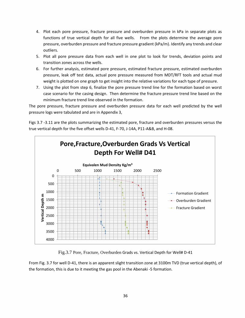
Figs 3.7 -3.11 are the plots summarizing the estimated pore, fracture and overburden pressures versus the

true vertical depth for the five offset wells D-41, F-70, J-14A, P11-A&B, and H-08.

Fig.3.7 Pore, Fracture, Overburden Grads vs. Vertical Depth for Well# D-41

From Fig. 3.7 for well D-41, there is an apparent slight transition zone at 3100m TVD (true vertical depth), of

the formation, this is due to it meeting the gas pool in the Abenaki -5 formation.

0

500

1000

1500

2000

2500

3000

3500

4000

0 500 1000 1500 2000 2500

Ve

rtic

al D

ep

th m

Equivalen Mud Density Kg/m³

Pore,Fracture,Overburden Grads Vs Vertical Depth For Well# D41

Formation Gradient

Overburden Gradient

Fracture Gradient

37

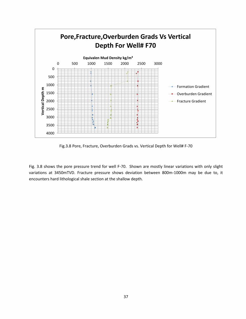
Fig.3.8 Pore, Fracture, Overburden Grads vs. Vertical Depth for Well# F-70

Fig. 3.8 shows the pore pressure trend for well F-70. Shown are mostly linear variations with only slight

variations at 3450mTVD. Fracture pressure shows deviation between 800m-1000m may be due to, it

encounters hard lithological shale section at the shallow depth.

0

500

1000

1500

2000

2500

3000

3500

4000

0 500 1000 1500 2000 2500 3000

Ve

rtic

al D

ep

th m

Equivalen Mud Density kg/m³

Pore,Fracture,Overburden Grads Vs Vertical Depth For Well# F70

Formation Gradient

Overburden Gradient

Fracture Gradient

38

Fig.3.9 Pore, Fracture, Overburden Grads vs. Vertical Depth for Well# J-14A

Fig. 3.9 summarizes the pore pressure variation for the well J-14A. Again, mostly linear variations with TVD

with small changes at 3250m. In this well, the fracture pressure predicted is closer to the pore pressure line

compared to other four wells.

Fig.3.10 Pore, Fracture Grads vs. Vertical Depth for Well# P11-A&B

0

500

1000

1500

2000

2500

3000

3500

4000

0 500 1000 1500 2000 2500

Ve

rtic

al D

ep

th m

Equivalen Mud Density kg/m³

Pore,Fracture,Overburden Grads Vs Vertical Depth For Well# J14 & J14A

Formation Gradient

Overburden Gradient

Fracture Gradient

0

500

1000

1500

2000

2500

3000

3500

4000

0 500 1000 1500 2000

Ve

rtic

al D

ep

th m

Equivalen Mud Density kg/m³

Pore,Fracture Grads Vs Vertical Depth For Well# P11-A&B

Formation Gradient

Fracture Gradient

39

Fig.3.10 shows for well P11-A7B, a deviated pore pressure point at the beginning this point will be omitted

when considering the final pore pressure prediction, the overburden resistance data is not plotted in the

pressure log.

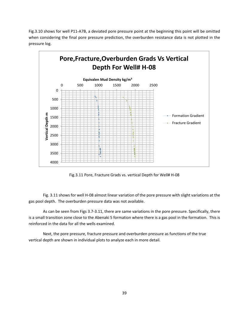
Fig.3.11 Pore, Fracture Grads vs. vertical Depth for Well# H-08

Fig. 3.11 shows for well H-08 almost linear variation of the pore pressure with slight variations at the

gas pool depth. The overburden pressure data was not available.

As can be seen from Figs 3.7-3.11, there are same variations in the pore pressure. Specifically, there

is a small transition zone close to the Abenaki 5 formation where there is a gas pool in the formation. This is

reinforced in the data for all the wells examined.

Next, the pore pressure, fracture pressure and overburden pressure as functions of the true

vertical depth are shown in individual plots to analyze each in more detail.

0

500

1000

1500

2000

2500

3000

3500

4000

0 500 1000 1500 2000 2500

Ve

rtic

al D

ep

th m

Equivalen Mud Density kg/m³

Pore,Fracture,Overburden Grads Vs Vertical Depth For Well# H-08

Formation Gradient

Fracture Gradient

40

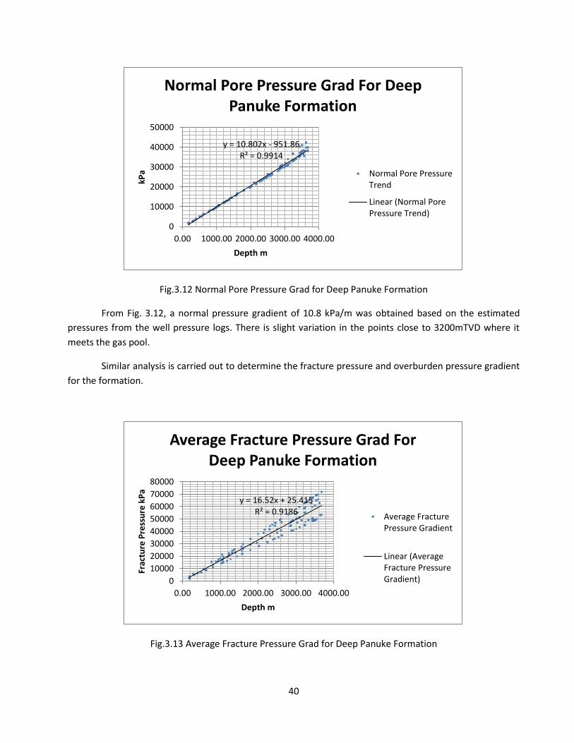
Fig.3.12 Normal Pore Pressure Grad for Deep Panuke Formation

From Fig. 3.12, a normal pressure gradient of 10.8 kPa/m was obtained based on the estimated

pressures from the well pressure logs. There is slight variation in the points close to 3200mTVD where it

meets the gas pool.

Similar analysis is carried out to determine the fracture pressure and overburden pressure gradient

for the formation.

Fig.3.13 Average Fracture Pressure Grad for Deep Panuke Formation

y = 10.802x - 951.86R² = 0.9914

0

10000

20000

30000

40000

50000

0.00 1000.00 2000.00 3000.00 4000.00

kPa

Depth m

Normal Pore Pressure Grad For Deep Panuke Formation

Normal Pore PressureTrend

Linear (Normal PorePressure Trend)

y = 16.52x + 25.415R² = 0.9186

0

10000

20000

30000

40000

50000

60000

70000

80000

0.00 1000.00 2000.00 3000.00 4000.00

Frac

ture

Pre

ssu

re k

Pa

Depth m

Average Fracture Pressure Grad For Deep Panuke Formation

Average FracturePressure Gradient

Linear (AverageFracture PressureGradient)

41

Fig. 3.13 shows the fracture pressure varies over a wider range with increase depth. The average

fracture pressure for the formation is extracted as 16.52KPa/m based on the estimated data from pressure

logs.

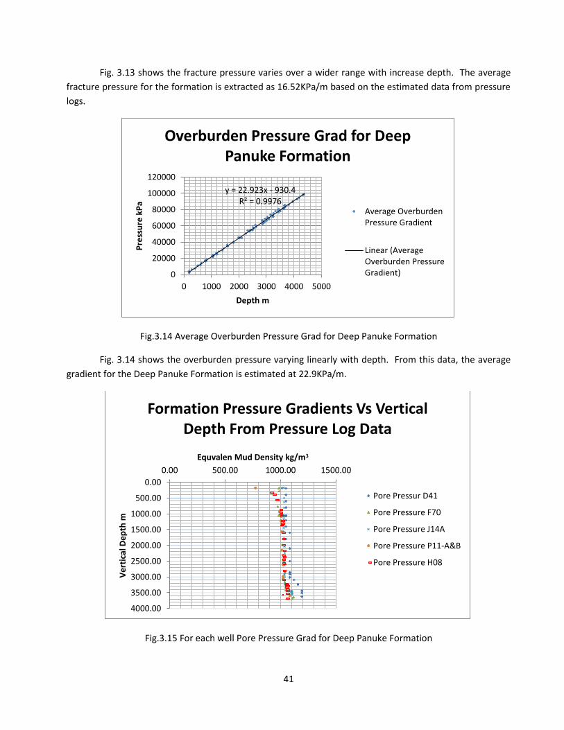
Fig.3.14 Average Overburden Pressure Grad for Deep Panuke Formation

Fig. 3.14 shows the overburden pressure varying linearly with depth. From this data, the average

gradient for the Deep Panuke Formation is estimated at 22.9KPa/m.

Fig.3.15 For each well Pore Pressure Grad for Deep Panuke Formation

y = 22.923x - 930.4R² = 0.9976

0

20000

40000

60000

80000

100000

120000

0 1000 2000 3000 4000 5000

Pre

ssu

re k

Pa

Depth m

Overburden Pressure Grad for Deep Panuke Formation

Average OverburdenPressure Gradient

Linear (AverageOverburden PressureGradient)

0.00

500.00

1000.00

1500.00

2000.00

2500.00

3000.00

3500.00

4000.00

0.00 500.00 1000.00 1500.00

Ve

rtic

al D

ep

th m

Equvalen Mud Density kg/m³

Formation Pressure Gradients Vs Vertical Depth From Pressure Log Data

Pore Pressur D41

Pore Pressure F70

Pore Pressure J14A

Pore Pressure P11-A&B

Pore Pressure H08

42

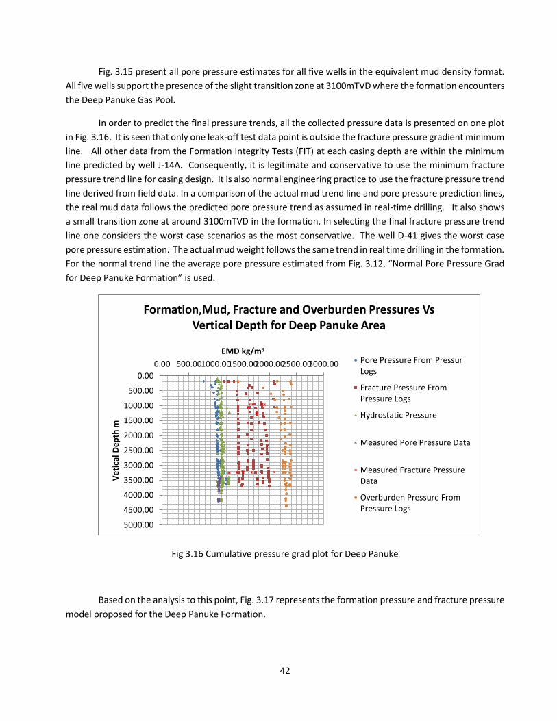
Fig. 3.15 present all pore pressure estimates for all five wells in the equivalent mud density format.

All five wells support the presence of the slight transition zone at 3100mTVD where the formation encounters

the Deep Panuke Gas Pool.

In order to predict the final pressure trends, all the collected pressure data is presented on one plot

in Fig. 3.16. It is seen that only one leak-off test data point is outside the fracture pressure gradient minimum

line. All other data from the Formation Integrity Tests (FIT) at each casing depth are within the minimum

line predicted by well J-14A. Consequently, it is legitimate and conservative to use the minimum fracture

pressure trend line for casing design. It is also normal engineering practice to use the fracture pressure trend

line derived from field data. In a comparison of the actual mud trend line and pore pressure prediction lines,

the real mud data follows the predicted pore pressure trend as assumed in real-time drilling. It also shows

a small transition zone at around 3100mTVD in the formation. In selecting the final fracture pressure trend

line one considers the worst case scenarios as the most conservative. The well D-41 gives the worst case

pore pressure estimation. The actual mud weight follows the same trend in real time drilling in the formation.

For the normal trend line the average pore pressure estimated from Fig. 3.12, “Normal Pore Pressure Grad

for Deep Panuke Formation” is used.

Fig 3.16 Cumulative pressure grad plot for Deep Panuke

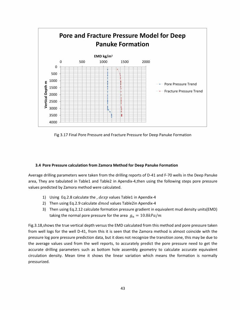
Based on the analysis to this point, Fig. 3.17 represents the formation pressure and fracture pressure

model proposed for the Deep Panuke Formation.

0.00

500.00

1000.00

1500.00

2000.00

2500.00

3000.00

3500.00

4000.00

4500.00

5000.00

0.00 500.001000.001500.002000.002500.003000.00

Ve

tica

l De

pth

m

EMD kg/m³

Formation,Mud, Fracture and Overburden Pressures Vs Vertical Depth for Deep Panuke Area

Pore Pressure From PressurLogs

Fracture Pressure FromPressure Logs

Hydrostatic Pressure

Measured Pore Pressure Data

Measured Fracture PressureData

Overburden Pressure FromPressure Logs

43

Fig 3.17 Final Pore Pressure and Fracture Pressure for Deep Panuke Formation

3.4 Pore Pressure calculation from Zamora Method for Deep Panuke Formation

Average drilling parameters were taken from the drilling reports of D-41 and F-70 wells in the Deep Panuke

area, They are tabulated in Table1 and Table2 in Apendix-4,then using the following steps pore pressure

values predicted by Zamora method were calculated.

1) Using Eq.2.8 calculate the , 𝑑𝑒𝑥𝑝 values Table1 in Apendix-4

2) Then using Eq.2.9 calculate 𝑑𝑚𝑜𝑑 values Table2in Apendix-4

3) Then using Eq.2.12 calculate formation pressure gradient in equivalent mud density units(EMD)

taking the normal pore pressure for the area 𝑔𝑛 = 10.8𝑘𝑃𝑎/𝑚

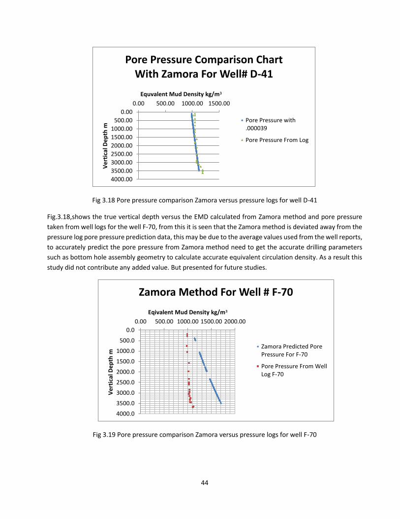
Fig.3.18,shows the true vertical depth versus the EMD calculated from this method and pore pressure taken

from well logs for the well D-41, from this it is seen that the Zamora method is almost coincide with the

pressure log pore pressure prediction data, but it does not recognize the transition zone, this may be due to

the average values used from the well reports, to accurately predict the pore pressure need to get the

accurate drilling parameters such as bottom hole assembly geometry to calculate accurate equivalent

circulation density. Mean time it shows the linear variation which means the formation is normally

pressurized.

0

500

1000

1500

2000

2500

3000

3500

4000

0 500 1000 1500 2000

Ve

rtic

al D

ep

th m

EMD kg/m³

Pore and Fracture Pressure Model for Deep Panuke Formation

Pore Pressure Trend

Fracture Pressure Trend

44

Fig 3.18 Pore pressure comparison Zamora versus pressure logs for well D-41

Fig.3.18,shows the true vertical depth versus the EMD calculated from Zamora method and pore pressure

taken from well logs for the well F-70, from this it is seen that the Zamora method is deviated away from the

pressure log pore pressure prediction data, this may be due to the average values used from the well reports,

to accurately predict the pore pressure from Zamora method need to get the accurate drilling parameters

such as bottom hole assembly geometry to calculate accurate equivalent circulation density. As a result this

study did not contribute any added value. But presented for future studies.

Fig 3.19 Pore pressure comparison Zamora versus pressure logs for well F-70

0.00

500.00

1000.00

1500.00

2000.00

2500.00

3000.00

3500.00

4000.00

0.00 500.00 1000.00 1500.00V

ert

ical

De

pth

m

Equvalent Mud Density kg/m³

Pore Pressure Comparison Chart With Zamora For Well# D-41

Pore Pressure with.000039

Pore Pressure From Log

0.0

500.0

1000.0

1500.0

2000.0

2500.0

3000.0

3500.0

4000.0

0.00 500.00 1000.00 1500.00 2000.00

Ve

rtic

al D

ep

th m

Eqivalent Mud Density kg/m³

Zamora Method For Well # F-70

Zamora Predicted PorePressure For F-70

Pore Pressure From WellLog F-70

45

4.0 Casing Design Calculation

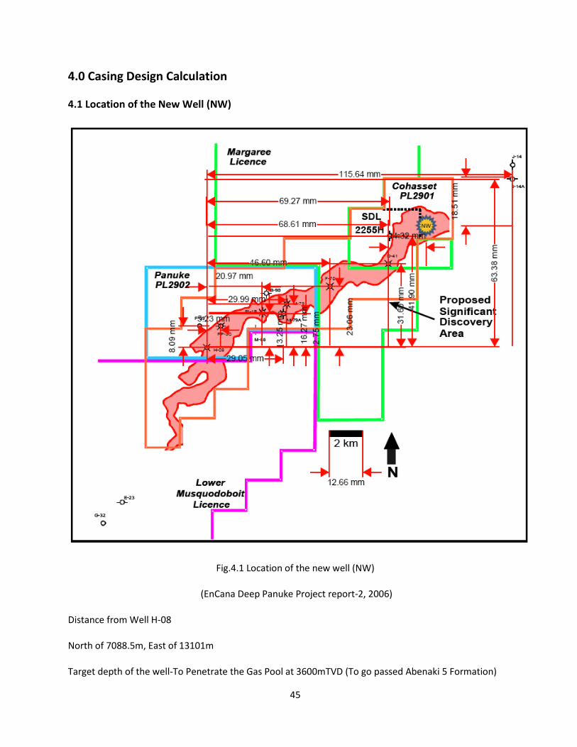
4.1 Location of the New Well (NW)

Fig.4.1 Location of the new well (NW)

(EnCana Deep Panuke Project report-2, 2006)

Distance from Well H-08

North of 7088.5m, East of 13101m

Target depth of the well-To Penetrate the Gas Pool at 3600mTVD (To go passed Abenaki 5 Formation)

46

4.2 Basic Design Considerations

Safety Factors for principle load calculations (As per Rabia 1987)

1.0 For Collapse Loading-0.85 to 1.125 2.0 For Burst Loading-1 to 1.1 3.0 For Tension Loading-1.6 to 1.8

Design load for collapse and burst should be considered first, then check for tension if needed, needs to correct for tension

Swab/Surge Pressure effect need to be considered

Pipe Sticking effect that happens when the pipe is longer(the tendency to stick in the formation) for normally pressured area & abnormally pressured area need to be checked

For normally pressurized area maximum differential pressure at which the casing can be run without severe pipe sticking 2000 psi to 2300 psi (13790kPa to 15859kPa) (as per Adams, 1985)

For abnormally pressured zones it is 3000psi to 3300psi (20684kPa to 22754kPa)

47

4.3 Casing Setting Depth Calculations and Factors Considered

Setting depths and number of casing strings depends on geological conditions and the protection of fresh water aquifers. In deep wells primary consideration is either given to the control of abnormal pressure and its isolation from weak shallow zones or to the control of salt beds which will tend to flow plastically.

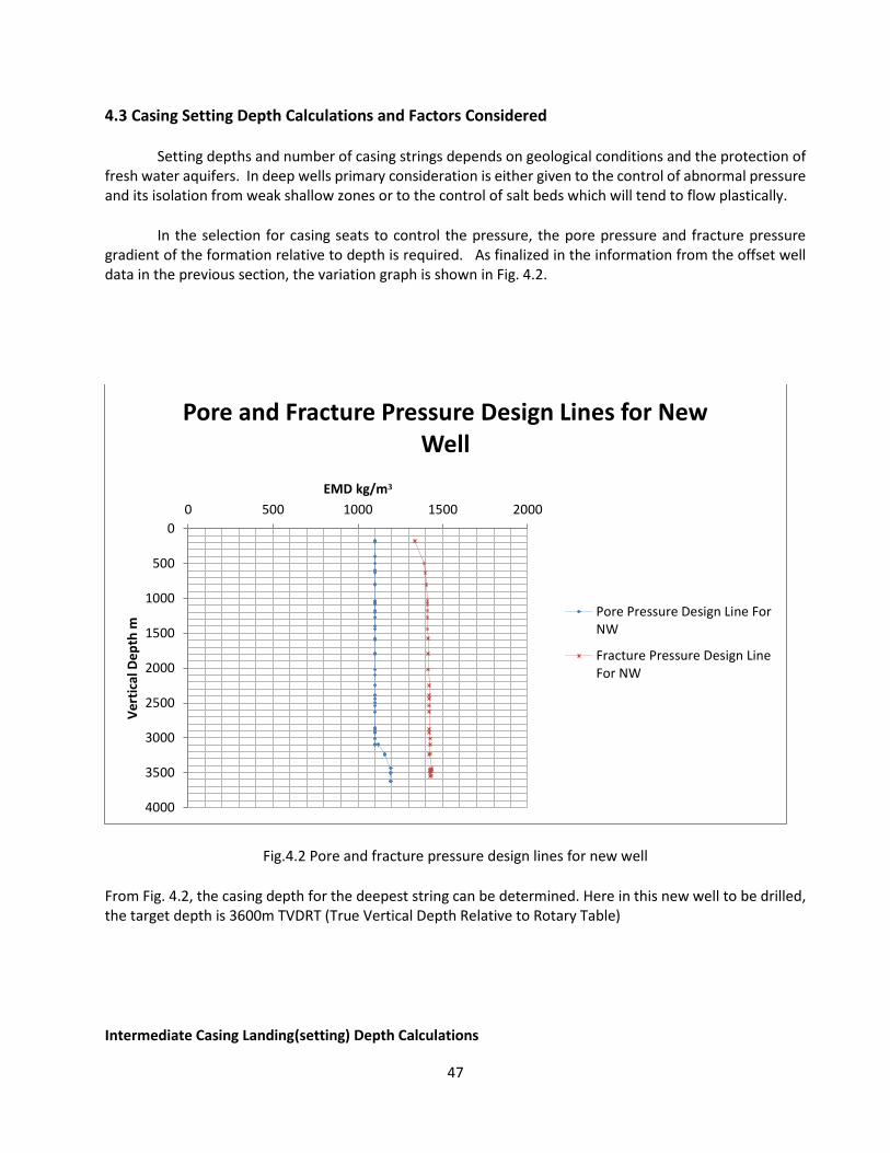
In the selection for casing seats to control the pressure, the pore pressure and fracture pressure gradient of the formation relative to depth is required. As finalized in the information from the offset well data in the previous section, the variation graph is shown in Fig. 4.2.

Fig.4.2 Pore and fracture pressure design lines for new well

From Fig. 4.2, the casing depth for the deepest string can be determined. Here in this new well to be drilled, the target depth is 3600m TVDRT (True Vertical Depth Relative to Rotary Table)

Intermediate Casing Landing(setting) Depth Calculations

0

500

1000

1500

2000

2500

3000

3500

4000

0 500 1000 1500 2000

Ve

rtic

al D

ep

th m

EMD kg/m³

Pore and Fracture Pressure Design Lines for New Well

Pore Pressure Design Line ForNW

Fracture Pressure Design LineFor NW

48

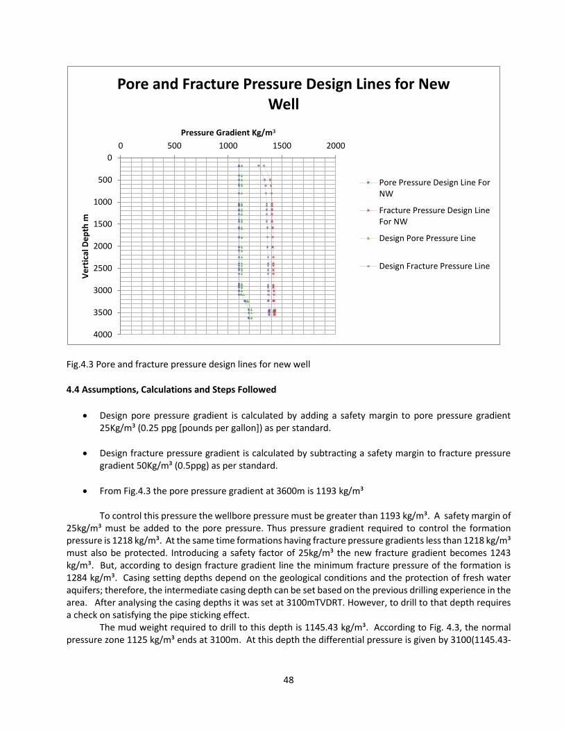
Fig.4.3 Pore and fracture pressure design lines for new well

4.4 Assumptions, Calculations and Steps Followed

Design pore pressure gradient is calculated by adding a safety margin to pore pressure gradient 25Kg/m³ (0.25 ppg [pounds per gallon]) as per standard.

Design fracture pressure gradient is calculated by subtracting a safety margin to fracture pressure gradient 50Kg/m³ (0.5ppg) as per standard.

From Fig.4.3 the pore pressure gradient at 3600m is 1193 kg/m³

To control this pressure the wellbore pressure must be greater than 1193 kg/m³. A safety margin of 25kg/m³ must be added to the pore pressure. Thus pressure gradient required to control the formation pressure is 1218 kg/m³. At the same time formations having fracture pressure gradients less than 1218 kg/m³ must also be protected. Introducing a safety factor of 25kg/m³ the new fracture gradient becomes 1243 kg/m³. But, according to design fracture gradient line the minimum fracture pressure of the formation is 1284 kg/m³. Casing setting depths depend on the geological conditions and the protection of fresh water aquifers; therefore, the intermediate casing depth can be set based on the previous drilling experience in the area. After analysing the casing depths it was set at 3100mTVDRT. However, to drill to that depth requires a check on satisfying the pipe sticking effect.

The mud weight required to drill to this depth is 1145.43 kg/m³. According to Fig. 4.3, the normal pressure zone 1125 kg/m³ ends at 3100m. At this depth the differential pressure is given by 3100(1145.43-

0

500

1000

1500

2000

2500

3000

3500

4000

0 500 1000 1500 2000

Ve

rtic

al D

ep

th m

Pressure Gradient Kg/m³

Pore and Fracture Pressure Design Lines for New Well

Pore Pressure Design Line ForNW

Fracture Pressure Design LineFor NW

Design Pore Pressure Line

Design Fracture Pressure Line

49

1125)*0.00981=621.3kPa which is outside of the 13790kPa – 15859kPa (as per Adams, 1985). This implies that there will not be any pipe sticking problem when drilling up to this depth.

If the above criterion was not satisfied, Eq.4.1 gives the maximum distance that can be drilled in this

formation without sticking the pipe.

∆P= Dh (Ym-Yf)*0.00981 (4.1)

where ∆P = Arbitral limit of differential pressure (kPa)

Ym =specific weight of drilling fluid (kg/m³)

Yf = specific weight of formation fluid (Kg/m³)

Dh =depth where normal zone end (m)

0.00981-Conversion Factor from kg/m³ to KPa

From the pipe sticking limit, now calculate the mud weight from Eq. xx to determine the depth from Fig. 4.3 to determine the equivalent mud density. In this design we do not have to do the reverse calculation as the requirement is satisfied.

Therefore the final setting depth for intermediate casing is 3100mTVD.

4.5 To check the pipe sticking test for the production casing

Drilling Mud Density at 3600mTVD=1217.72 kg/m³

Pressure Differential at this depth=3100(1217.72-1125)*0.00981=2819.7KPa which is less than 13790kPa to 15859kPa (as per Adams, 1985) this implies that there will not be any pipe sticking problem when drilling up to this depth.

Therefore final settling depth for production casing is 3600mTVD.

4.6 Surface Casing String Settling Depth Surface casing is subjected to abnormal pressures due to a kick arising from the deepest section of

the hole, if a kick occurs and the shut in casing pressure plus the drilling fluid hydrostatic pressure exceeds the fracture resistance pressure of the formation at the casing shoe, fracturing or an underground blowout can occur, thus surface casing depth needs to be selected to contain this kick imposed pressure. Other factor need to be considered is protection of fresh water aquifers. Aquifer normally occurs in the range of 600-1500m.

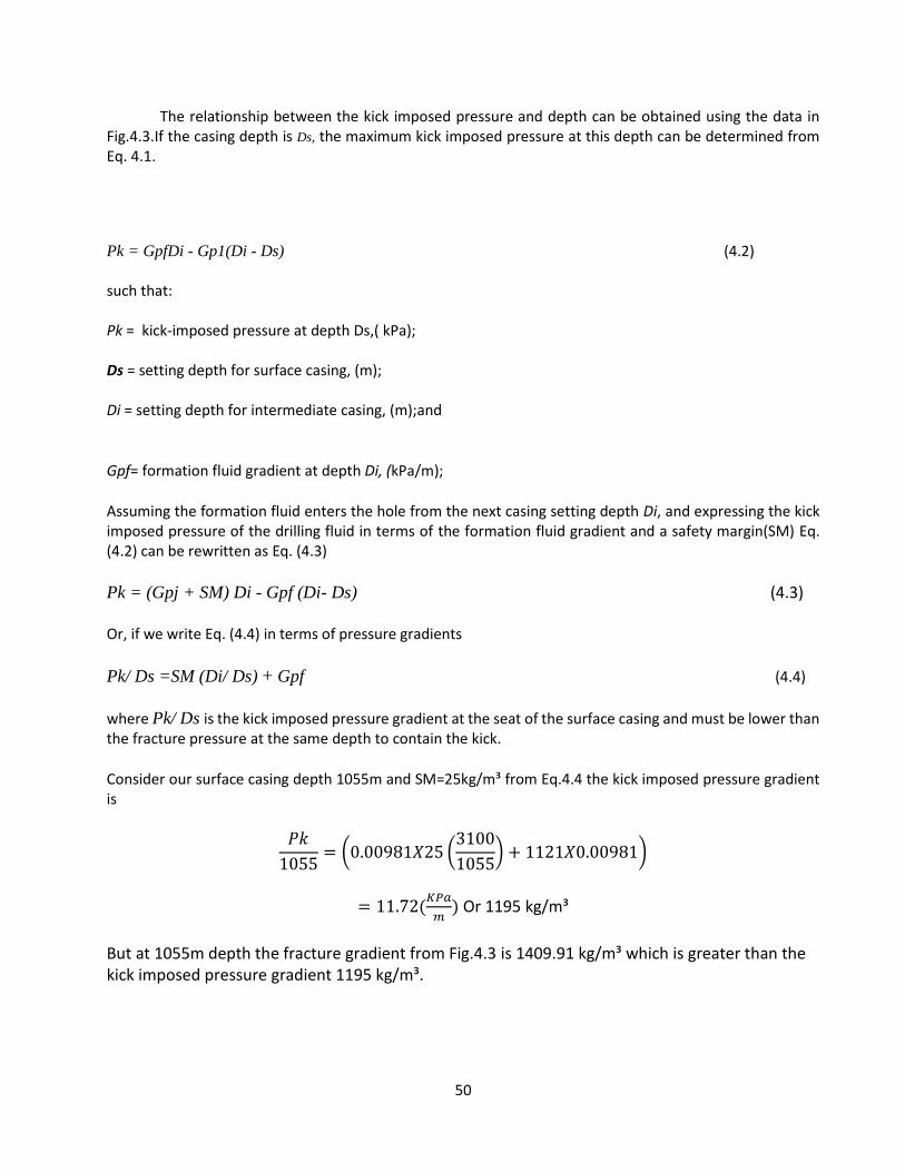
50

The relationship between the kick imposed pressure and depth can be obtained using the data in Fig.4.3.If the casing depth is Ds, the maximum kick imposed pressure at this depth can be determined from Eq. 4.1.

Pk = GpfDi - Gp1(Di - Ds) (4.2) such that: Pk = kick-imposed pressure at depth Ds,( kPa); Ds = setting depth for surface casing, (m); Di = setting depth for intermediate casing, (m);and

Gpf= formation fluid gradient at depth Di, (kPa/m);

Assuming the formation fluid enters the hole from the next casing setting depth Di, and expressing the kick imposed pressure of the drilling fluid in terms of the formation fluid gradient and a safety margin(SM) Eq. (4.2) can be rewritten as Eq. (4.3)

Pk = (Gpj + SM) Di - Gpf (Di- Ds) (4.3)

Or, if we write Eq. (4.4) in terms of pressure gradients

Pk/ Ds =SM (Di/ Ds) + Gpf (4.4)

where Pk/ Ds is the kick imposed pressure gradient at the seat of the surface casing and must be lower than the fracture pressure at the same depth to contain the kick.

Consider our surface casing depth 1055m and SM=25kg/m³ from Eq.4.4 the kick imposed pressure gradient is

𝑃𝑘

1055= (0.00981𝑋25 (

3100

1055) + 1121𝑋0.00981)

= 11.72(𝐾𝑃𝑎

𝑚) Or 1195 kg/m³

But at 1055m depth the fracture gradient from Fig.4.3 is 1409.91 kg/m³ which is greater than the kick imposed pressure gradient 1195 kg/m³.

51

Therefore, the selected depth for surface casing satisfies the requirement, i.e. satisfies the dual requirements to prevent underground blowouts and to protect fresh water aquifers.

4.7 Conductor Pipe Setting Depth

This settling depth usually is determined by the drilling incidents and protection of water aquifers at shallow depths in the formation. Severe lost circulation zones often occur at these shallow depths. Other factors considered include unconsolidated formations and gas traps at these shallow depth areas. After an analysis of the area for the well the conductor casing depth is set at 182mTVDRT. Fig. 4.4 summarizes the depth heights set for each casing.

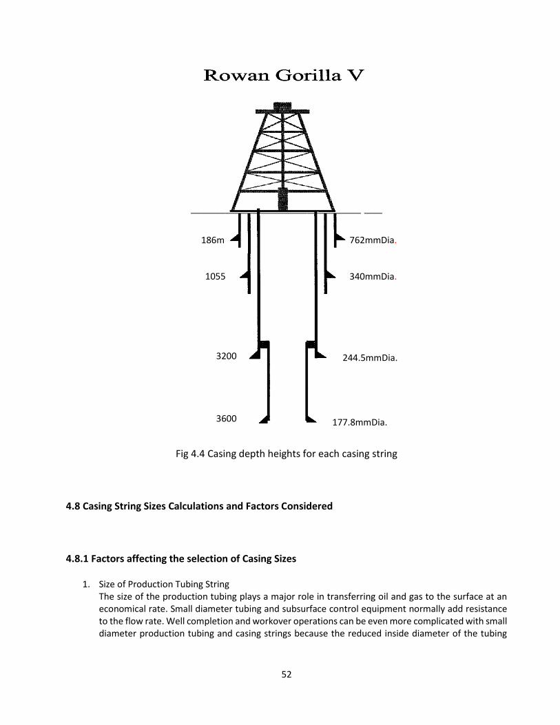
52

Fig 4.4 Casing depth heights for each casing string

4.8 Casing String Sizes Calculations and Factors Considered

4.8.1 Factors affecting the selection of Casing Sizes

1. Size of Production Tubing String The size of the production tubing plays a major role in transferring oil and gas to the surface at an economical rate. Small diameter tubing and subsurface control equipment normally add resistance to the flow rate. Well completion and workover operations can be even more complicated with small diameter production tubing and casing strings because the reduced inside diameter of the tubing

186m

1055

m

3200

m

3600

m

762mmDia.

340mmDia.

244.5mmDia.

177.8mmDia.

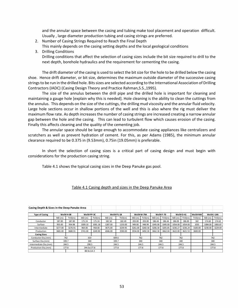
53

and the annular space between the casing and tubing make tool placement and operation difficult. Usually , large diameter production tubing and casing strings are preferred.

2. Number of Casing Strings Required to Reach the Final Depth This mainly depends on the casing setting depths and the local geological conditions

3. Drilling Conditions Drilling conditions that affect the selection of casing sizes include the bit size required to drill to the next depth, borehole hydraulics and the requirement for cementing the casing. The drift diameter of the casing is used to select the bit size for the hole to be drilled below the casing

shoe. Hence drift diameter, or bit size, determines the maximum outside diameter of the successive casing strings to be run in the drilled hole. Bits sizes are selected according to the International Association of Drilling Contractors (IADC) (Casing Design Theory and Practice Rahman,S.S.,1995).

The size of the annulus between the drill pipe and the drilled hole is important for cleaning and maintaining a gauge hole [explain why this is needed]. Hole cleaning is the ability to clean the cuttings from the annulus. This depends on the size of the cuttings, the drilling mud viscosity and the annular fluid velocity. Large hole sections occur in shallow portions of the well and this is also where the rig must deliver the maximum flow rate. As depth increases the number of casing strings are increased creating a narrow annular gap between the hole and the casing. This can lead to turbulent flow which causes erosion of the casing. Finally this affects cleaning and the quality of the cementing job.

The annular space should be large enough to accommodate casing appliances like centralizers and scratchers as well as prevent hydration of cement. For this, as per Adams (1985), the minimum annular clearance required to be 0.375 in (9.53mm), 0.75in (19.05mm) is preferable.

In short the selection of casing sizes is a critical part of casing design and must begin with

considerations for the production casing string.

Table 4.1 shows the typical casing sizes in the Deep Panuke gas pool.

Table 4.1 Casing depth and sizes in the Deep Panuke Area

Casing Depth & Sizes in the Deep Panuke Area

Type of Casing Well# NW

MD (m) TVD(m) MD (m) TVD(m) MD (m) TVD(m) MD (m) TVD(m) MD (m) TVD(m) MD (m) TVD(m) TVD(m) MD (m) TVD(m)

Conductor 187.00 187.00 175.24 175.24 182.50 182.49 203.00 203.00 186.44 186.44 186.00 186.00 182 174.60 174.62

Surface 955.00 954.98 1009.10 1001.18 1287.00 1233.00 949.00 948.99 1045.00 1045.00 1054.00 1054.00 1055 1084.00 1083.87

Intermediate 3277.00 3276.91 964.00 958.00 3675.00 3239.95 3261.00 3260.58 3206.30 3205.85 3236.27 3236.24 3100.00 3230.00 3229.69

Production 3681.00 3680.91 3741.00 3249.90 4046.00 3590.00 3934.00 3492.30 3662.30 3662.04 3622.00 3621.53 3600.00

Casing Sizes

Conductor Dia.(mm)

Surface Dia.(mm)

Intermediate Dia.(mm)

Production Dia.(mm)

Well# J-14A

762

339.7

244.5

177.8

610

340

298.5

244.5x177.8

Well# H-08 Well# PP-3C Well# P1-1B Well# M-79A Well# F-70 Well# D-41

762

340

244.5

177.8

88.9x114.3

609.6

339.7

244.5

177.8

762

340

244.5

177.8

762

340

244.5

177.8

762

340

244.5

177.8

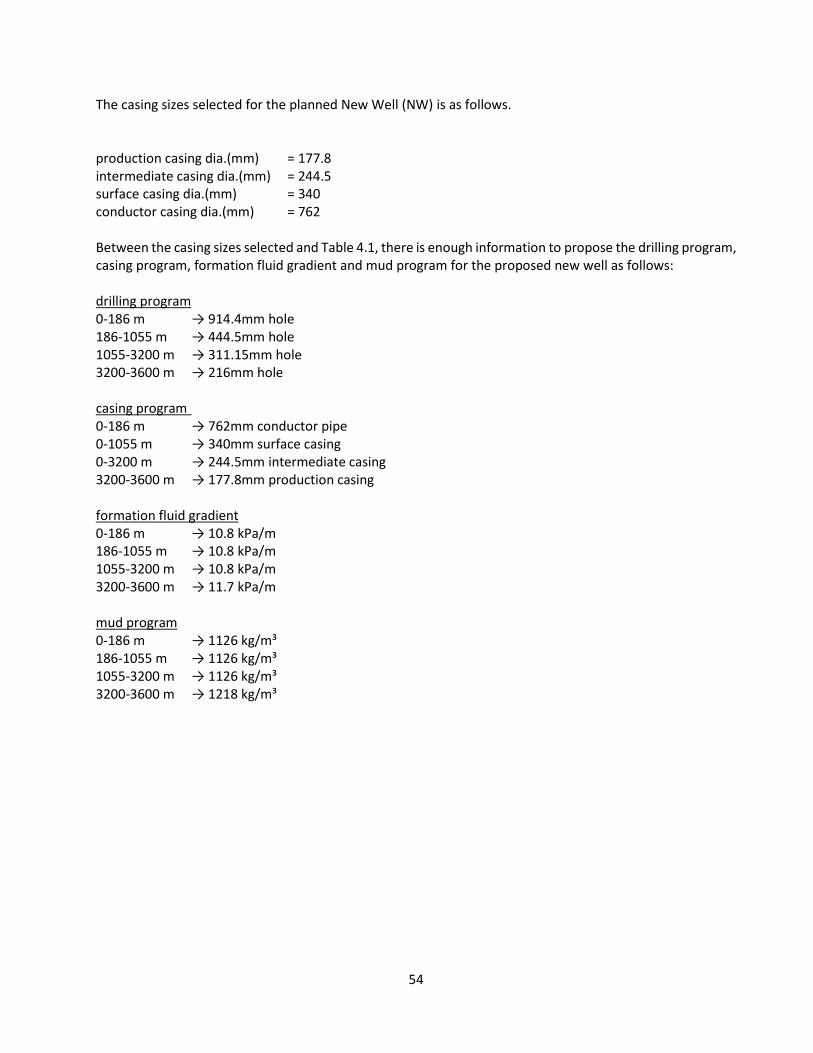
54

The casing sizes selected for the planned New Well (NW) is as follows.

production casing dia.(mm) = 177.8 intermediate casing dia.(mm) = 244.5 surface casing dia.(mm) = 340 conductor casing dia.(mm) = 762 Between the casing sizes selected and Table 4.1, there is enough information to propose the drilling program, casing program, formation fluid gradient and mud program for the proposed new well as follows: drilling program 0-186 m → 914.4mm hole 186-1055 m → 444.5mm hole 1055-3200 m → 311.15mm hole 3200-3600 m → 216mm hole casing program 0-186 m → 762mm conductor pipe 0-1055 m → 340mm surface casing 0-3200 m → 244.5mm intermediate casing 3200-3600 m → 177.8mm production casing formation fluid gradient 0-186 m → 10.8 kPa/m 186-1055 m → 10.8 kPa/m 1055-3200 m → 10.8 kPa/m 3200-3600 m → 11.7 kPa/m mud program 0-186 m → 1126 kg/m³ 186-1055 m → 1126 kg/m³ 1055-3200 m → 1126 kg/m³ 3200-3600 m → 1218 kg/m³

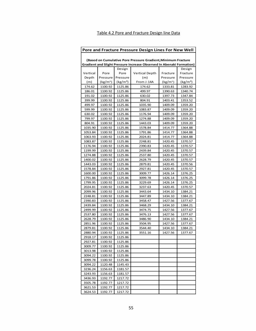
55

Table 4.2 Pore and Fracture Design line Data

Vertical

Depth

(m)

Pore

Pressure

(kg/m³)

Design

Pore

Pressure

(kg/m³)

Vertical Depth

(m)

From J-14A

Fracture

Pressure

(kg/m³)

Design

Fracture

Pressure

(kg/m³)

174.62 1100.92 1125.86 174.62 1333.81 1283.92

186.01 1100.92 1125.86 499.97 1390.63 1340.74

191.02 1100.92 1125.86 630.02 1397.73 1347.84

399.99 1100.92 1125.86 804.91 1403.41 1353.52

499.97 1100.92 1125.86 1035.90 1409.09 1359.20

599.99 1100.92 1125.86 1083.87 1409.09 1359.20

630.02 1100.92 1125.86 1176.94 1409.09 1359.20

799.97 1100.92 1125.86 1274.88 1409.09 1359.20

804.91 1100.92 1125.86 1443.03 1409.09 1359.20

1035.90 1100.92 1125.86 1578.84 1414.77 1364.88

1053.84 1100.92 1125.86 1791.86 1414.77 1364.88

1063.93 1100.92 1125.86 2024.81 1414.77 1364.88

1083.87 1100.92 1125.86 2248.81 1420.45 1370.57

1176.94 1100.92 1125.86 2390.83 1420.45 1370.57

1199.99 1100.92 1125.86 2439.84 1420.45 1370.57

1274.88 1100.92 1125.86 2537.80 1420.45 1370.57

1400.02 1100.92 1125.86 2628.79 1420.45 1370.57

1443.03 1100.92 1125.86 2879.81 1420.45 1370.56

1578.84 1100.92 1125.86 2927.81 1420.45 1370.57

1600.00 1100.92 1125.86 3009.77 1426.14 1376.25

1791.86 1100.92 1125.86 3099.78 1426.14 1376.25

1799.95 1100.92 1125.86 3229.69 1426.14 1376.25

2024.81 1100.92 1125.86 3237.63 1420.45 1370.57

2099.96 1100.92 1125.86 3443.64 1434.10 1384.21

2248.81 1100.92 1125.86 3447.89 1434.10 1384.21

2390.83 1100.92 1125.86 3458.47 1427.56 1377.67

2439.84 1100.92 1125.86 3468.29 1434.10 1384.21

2499.99 1100.92 1125.86 3474.75 1427.56 1377.67

2537.80 1100.92 1125.86 3476.13 1427.56 1377.67

2628.79 1100.92 1125.86 3486.90 1434.10 1384.21

2851.96 1100.92 1125.86 3504.95 1427.56 1377.67

2879.81 1100.92 1125.86 3544.40 1434.10 1384.21

2880.94 1100.92 1125.86 3551.16 1427.56 1377.67

2918.17 1100.92 1125.86

2927.81 1100.92 1125.86

3009.77 1100.92 1125.86

3013.98 1100.92 1125.86

3094.22 1100.92 1125.86

3099.78 1100.92 1125.86

3094.22 1120.48 1145.43

3236.24 1156.63 1181.57

3243.93 1156.63 1181.57

3436.93 1192.77 1217.72

3505.78 1192.77 1217.72

3621.53 1192.77 1217.72

3624.53 1192.77 1217.72

(Based on Cumulative Pore Pressure Gradient,Minimum Fracture

Gradient and Slight Pressure Increase Observed In Abenaki Formation)

Pore and Fracture Pressure Design Lines For New Well

56

4.9 Selection of Casing Weight Grade and Couplings

Once the number of casing strings required to complete a hole is established as well as the respective

setting depths and outside diameters the nominal weight, steel grade and couplings of each of these strings has to be determined. Normal practice is to design it to withstand the maximum load that arises during casing landing, drilling and production operations. Generally, it is not possible to forecast the tensile, collapse and burst loads during the life of the casing. Therefore, when designing the casings worse case scenarios during the life span are considered. Properties of the casings deteriorate with the time due to wear and corrosion. In order to compensate for this safety factors are introduced, As per Rabia (1987) common safety factors for the three principal loads are 0.85-1.125 for collapse, 1-1.1 for burst, and 1.6-1.8 for tension.

In order to obtain the most economical casing design, combinations of casing strings with different

nominal weights, grades and couplings are used. Normally, by selecting the string with the lowest possible weight per foot of steel and the lowest coupling grades which meets the design load criteria, the most economical casing design can be achieved.

Loading conditions vary for each type of casing string as they serve different purposes. For example

the casing head housing is generally installed on the conductor pipe so it is subjected to the cumulative compressional loads from the weight of the subsequent casing strings. Consequently, the design of the conductor pipe can be done only after the weights of the successive casings are determined.

In order to select the steel grades a graphical method introduced by Goins et al (1965, 1966), then

modified by Prentice (1970) and Rabia (1987) is applied. A graph of loads (collapse or burst) versus depth is first constructed then the strength values of available steel grades are plotted as vertical lines. Then, steel grades which satisfy the maximum existing load requirements of collapse and burst are chosen.

The normal design load for collapse and burst should be considered first. Once weights, grades and

sectional lengths that satisfy both burst and collapse loads are determined, the tension load requirements are then evaluated. If needed pipe section can be upgraded accordingly. The final step is to check the biaxial effect on collapse and burst load. If the strength in any part of the section is lower than the potential load, that particular section should be upgraded and the design process repeated. Selection of Surface Casing Weight Grade and Couplings surface casing size: 340mm (13 3/8 in) surface casing depth: 1055m it is cemented back to the surface principal loads considered: collapse, burst and biaxial effects. Since the casing is cemented back to the surface buckling effects are ignored. 4.9.1 Collapse Failure

Failure in collapse arises from the differential pressure between the hydrostatic pressure heads in the annulus and casing. The differential pressure is maximum at the casing shoe and gauge at the surface. The worst case scenario happens if the casing is run empty or if a lost circulation zone is encountered during the drilling of the next interval(section). In shallow areas if a severe lost circulation zone is met close to the bottom of the next interval and no other permeable zones exist above the lost circulation zone, it is possible

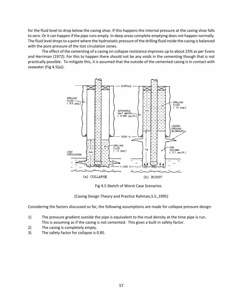
57

for the fluid level to drop below the casing shoe. If this happens the internal pressure at the casing shoe falls to zero. Or it can happen if the pipe runs empty. In deep areas complete emptying does not happen normally. The fluid level drops to a point where the hydrostatic pressure of the drilling fluid inside the casing is balanced with the pore pressure of the lost circulation zones.

The effect of the cementing of a casing on collapse resistance improves up to about 23% as per Evans and Herriman (1972). For this to happen there should not be any voids in the cementing though that is not practically possible. To mitigate this, it is assumed that the outside of the cemented casing is in contact with seawater (Fig 4.5(a)).

Fig 4.5 Sketch of Worst Case Scenarios

(Casing Design Theory and Practice Rahman,S.S.,1995)

Considering the factors discussed so far, the following assumptions are made for collapse pressure design: 1) The pressure gradient outside the pipe is equivalent to the mud density at the time pipe is run.

This is assuming as if the casing is not cemented. This gives a built in safety factor. 2) The casing is completely empty. 3) The safety factor for collapse is 0.85.

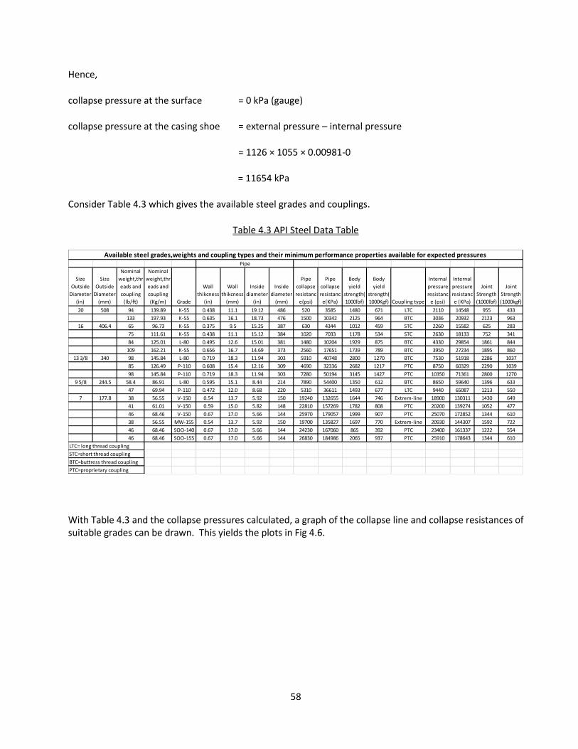
58

Hence,

collapse pressure at the surface = 0 kPa (gauge)

collapse pressure at the casing shoe = external pressure – internal pressure

= 1126 × 1055 × 0.00981-0

= 11654 kPa

Consider Table 4.3 which gives the available steel grades and couplings.

Table 4.3 API Steel Data Table

With Table 4.3 and the collapse pressures calculated, a graph of the collapse line and collapse resistances of suitable grades can be drawn. This yields the plots in Fig 4.6.

Size

Outside

Diameter

(in)

Size

Outside

Diameter

(mm)

Nominal

weight,thr

eads and

coupling

(lb/ft)

Nominal

weight,thr

eads and

coupling

(Kg/m) Grade

Wall

thikcness

(in)

Wall

thikcness

(mm)

Inside

diameter

(in)

Inside

diameter

(mm)

Pipe

collapse

resistanc

e(psi)

Pipe

collapse

resistanc

e(KPa)

Body

yield

strength(

1000lbf)

Body

yield

strength(

1000Kgf) Coupling type

Internal

pressure

resistanc

e (psi)

Internal

pressure

resistanc

e (KPa)

Joint

Strength

(1000lbf)

Joint

Strength

(1000kgf)

20 508 94 139.89 K-55 0.438 11.1 19.12 486 520 3585 1480 671 LTC 2110 14548 955 433

133 197.93 K-55 0.635 16.1 18.73 476 1500 10342 2125 964 BTC 3036 20932 2123 963

16 406.4 65 96.73 K-55 0.375 9.5 15.25 387 630 4344 1012 459 STC 2260 15582 625 283

75 111.61 K-55 0.438 11.1 15.12 384 1020 7033 1178 534 STC 2630 18133 752 341

84 125.01 L-80 0.495 12.6 15.01 381 1480 10204 1929 875 BTC 4330 29854 1861 844

109 162.21 K-55 0.656 16.7 14.69 373 2560 17651 1739 789 BTC 3950 27234 1895 860

13 3/8 340 98 145.84 L-80 0.719 18.3 11.94 303 5910 40748 2800 1270 BTC 7530 51918 2286 1037

85 126.49 P-110 0.608 15.4 12.16 309 4690 32336 2682 1217 PTC 8750 60329 2290 1039

98 145.84 P-110 0.719 18.3 11.94 303 7280 50194 3145 1427 PTC 10350 71361 2800 1270

9 5/8 244.5 58.4 86.91 L-80 0.595 15.1 8.44 214 7890 54400 1350 612 BTC 8650 59640 1396 633

47 69.94 P-110 0.472 12.0 8.68 220 5310 36611 1493 677 LTC 9440 65087 1213 550

7 177.8 38 56.55 V-150 0.54 13.7 5.92 150 19240 132655 1644 746 Extrem-line 18900 130311 1430 649

41 61.01 V-150 0.59 15.0 5.82 148 22810 157269 1782 808 PTC 20200 139274 1052 477

46 68.46 V-150 0.67 17.0 5.66 144 25970 179057 1999 907 PTC 25070 172852 1344 610

38 56.55 MW-155 0.54 13.7 5.92 150 19700 135827 1697 770 Extrem-line 20930 144307 1592 722

46 68.46 SOO-140 0.67 17.0 5.66 144 24230 167060 865 392 PTC 23400 161337 1222 554

46 68.46 SOO-155 0.67 17.0 5.66 144 26830 184986 2065 937 PTC 25910 178643 1344 610

PTC=proprietary coupling

Pipe

Available steel grades,weights and coupling types and their minimum performance properties available for expected pressures

LTC= long thread coupling

STC=short thread coupling

BTC=buttress thread coupling

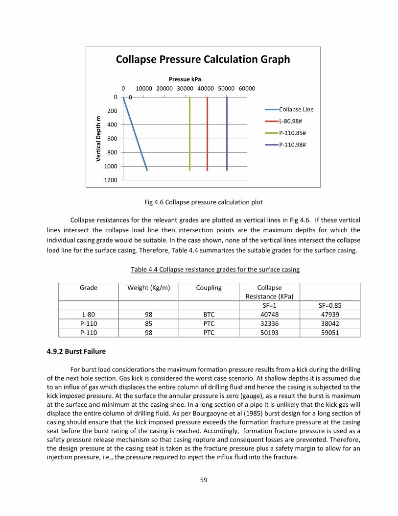
59

Fig 4.6 Collapse pressure calculation plot

Collapse resistances for the relevant grades are plotted as vertical lines in Fig 4.6. If these vertical

lines intersect the collapse load line then intersection points are the maximum depths for which the

individual casing grade would be suitable. In the case shown, none of the vertical lines intersect the collapse

load line for the surface casing. Therefore, Table 4.4 summarizes the suitable grades for the surface casing.

Table 4.4 Collapse resistance grades for the surface casing

Grade Weight (Kg/m) Coupling Collapse Resistance (KPa)

SF=1 SF=0.85

L-80 98 BTC 40748 47939

P-110 85 PTC 32336 38042

P-110 98 PTC 50193 59051

4.9.2 Burst Failure

For burst load considerations the maximum formation pressure results from a kick during the drilling of the next hole section. Gas kick is considered the worst case scenario. At shallow depths it is assumed due to an influx of gas which displaces the entire column of drilling fluid and hence the casing is subjected to the kick imposed pressure. At the surface the annular pressure is zero (gauge), as a result the burst is maximum at the surface and minimum at the casing shoe. In a long section of a pipe it is unlikely that the kick gas will displace the entire column of drilling fluid. As per Bourgaoyne et al (1985) burst design for a long section of casing should ensure that the kick imposed pressure exceeds the formation fracture pressure at the casing seat before the burst rating of the casing is reached. Accordingly, formation fracture pressure is used as a safety pressure release mechanism so that casing rupture and consequent losses are prevented. Therefore, the design pressure at the casing seat is taken as the fracture pressure plus a safety margin to allow for an injection pressure, i.e., the pressure required to inject the influx fluid into the fracture.

00

200

400

600

800

1000

1200

0 10000 20000 30000 40000 50000 60000

Ve

rtic

al D

ep

th m

Pressue kPa

Collapse Pressure Calculation Graph

Collapse Line

L-80,98#

P-110,85#

P-110,98#

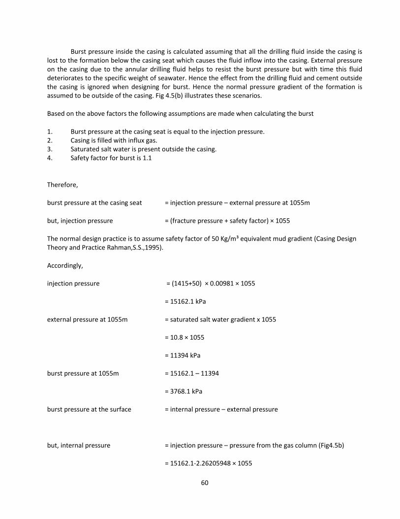
60

Burst pressure inside the casing is calculated assuming that all the drilling fluid inside the casing is lost to the formation below the casing seat which causes the fluid inflow into the casing. External pressure on the casing due to the annular drilling fluid helps to resist the burst pressure but with time this fluid deteriorates to the specific weight of seawater. Hence the effect from the drilling fluid and cement outside the casing is ignored when designing for burst. Hence the normal pressure gradient of the formation is assumed to be outside of the casing. Fig 4.5(b) illustrates these scenarios.

Based on the above factors the following assumptions are made when calculating the burst

1. Burst pressure at the casing seat is equal to the injection pressure. 2. Casing is filled with influx gas. 3. Saturated salt water is present outside the casing. 4. Safety factor for burst is 1.1

Therefore,

burst pressure at the casing seat = injection pressure – external pressure at 1055m

but, injection pressure = (fracture pressure + safety factor) × 1055

The normal design practice is to assume safety factor of 50 Kg/m³ equivalent mud gradient (Casing Design Theory and Practice Rahman,S.S.,1995).

Accordingly,

injection pressure = (1415+50) × 0.00981 × 1055

= 15162.1 kPa

external pressure at 1055m = saturated salt water gradient x 1055

= 10.8 × 1055

= 11394 kPa

burst pressure at 1055m = 15162.1 – 11394

= 3768.1 kPa

burst pressure at the surface = internal pressure – external pressure

but, internal pressure = injection pressure – pressure from the gas column (Fig4.5b)

= 15162.1-2.26205948 × 1055

61

= 12776 kPa

Therefore, burst pressure at surface = 12776 – 0

=12776 kPa

Fig. 4.7 shows this burst load on Fig 4.6 (at the surface 12776 kPa and 3768 KPa at 1055m depth).

Fig 4.7 Collapse Pressure calculation plot

Table 4.5 summarizes the suitable grades for surface casing based on burst loading.

Table 4.5 Burst resistance of grades for the surface casing

Grade Weight (Kg/m) Coupling Burst Resistance (KPa)

SF=1 SF=1.1

L-80 98 BTC 51918 47198

P-110 85 PTC 60329 54845

P-110 98 PTC 71361 64874

Table 4.5 Burst resistance grades

Plotting these burst resistance lines on the Fig 4.7 yields Fig. 4.8.

0

200

400

600

800

1000

1200

0 20000 40000 60000

Ve

rtic

al D

ep

th m

Pressue kPa

Collapse Pressure Calculation Graph

Collapse Line

L-80,98#

P-110,85#

P-110,98#

Burst Load Line

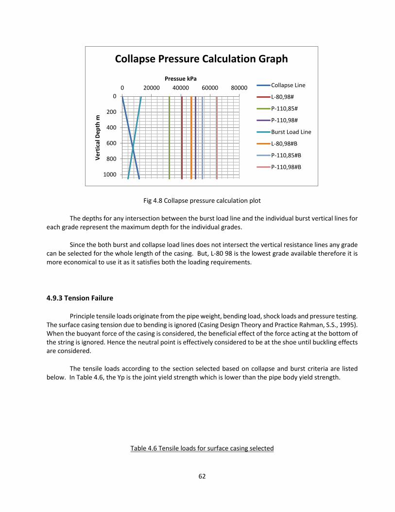
62

Fig 4.8 Collapse pressure calculation plot

The depths for any intersection between the burst load line and the individual burst vertical lines for each grade represent the maximum depth for the individual grades.

Since the both burst and collapse load lines does not intersect the vertical resistance lines any grade can be selected for the whole length of the casing. But, L-80 98 is the lowest grade available therefore it is more economical to use it as it satisfies both the loading requirements.

4.9.3 Tension Failure

Principle tensile loads originate from the pipe weight, bending load, shock loads and pressure testing. The surface casing tension due to bending is ignored (Casing Design Theory and Practice Rahman, S.S., 1995). When the buoyant force of the casing is considered, the beneficial effect of the force acting at the bottom of the string is ignored. Hence the neutral point is effectively considered to be at the shoe until buckling effects are considered.

The tensile loads according to the section selected based on collapse and burst criteria are listed below. In Table 4.6, the Yp is the joint yield strength which is lower than the pipe body yield strength.

Table 4.6 Tensile loads for surface casing selected

0

200

400

600

800

1000

0 20000 40000 60000 80000

Ve

rtic

al D

ep

th m

Pressue kPa

Collapse Pressure Calculation Graph

Collapse Line

L-80,98#

P-110,85#

P-110,98#

Burst Load Line

L-80,98#B

P-110,85#B

P-110,98#B

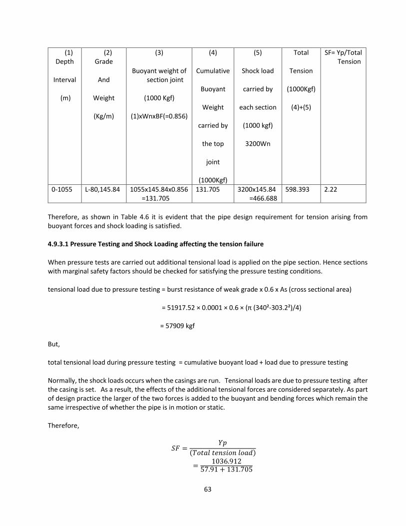
63

(1) Depth

Interval

(m)

(2) Grade

And

Weight

(Kg/m)

(3)

Buoyant weight of section joint

(1000 Kgf)

(1)xWnxBF(=0.856)

(4)

Cumulative

Buoyant

Weight

carried by

the top

joint

(1000Kgf)

(5)

Shock load

carried by

each section

(1000 kgf)

3200Wn

Total

Tension

(1000Kgf)

(4)+(5)

SF= Yp/Total Tension

0-1055 L-80,145.84 1055x145.84x0.856=131.705

131.705 3200x145.84=466.688

598.393 2.22

Therefore, as shown in Table 4.6 it is evident that the pipe design requirement for tension arising from buoyant forces and shock loading is satisfied.

4.9.3.1 Pressure Testing and Shock Loading affecting the tension failure

When pressure tests are carried out additional tensional load is applied on the pipe section. Hence sections with marginal safety factors should be checked for satisfying the pressure testing conditions.

tensional load due to pressure testing = burst resistance of weak grade x 0.6 x As (cross sectional area)

= 51917.52 × 0.0001 × 0.6 × (π (340²-303.2²)/4)

= 57909 kgf

But,

total tensional load during pressure testing = cumulative buoyant load + load due to pressure testing

Normally, the shock loads occurs when the casings are run. Tensional loads are due to pressure testing after the casing is set. As a result, the effects of the additional tensional forces are considered separately. As part of design practice the larger of the two forces is added to the buoyant and bending forces which remain the same irrespective of whether the pipe is in motion or static.

Therefore,

𝑆𝐹 =𝑌𝑝

(𝑇𝑜𝑡𝑎𝑙 𝑡𝑒𝑛𝑠𝑖𝑜𝑛 𝑙𝑜𝑎𝑑)

=1036.912

57.91 + 131.705

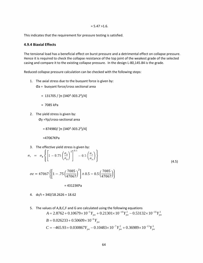
64

= 5.47 ˃1.6.

This indicates that the requirement for pressure testing is satisfied.

4.9.4 Biaxial Effects

The tensional load has a beneficial effect on burst pressure and a detrimental effect on collapse pressure. Hence it is required to check the collapse resistance of the top joint of the weakest grade of the selected casing and compare it to the existing collapse pressure. In the design L-80,145.84 is the grade.

Reduced collapse pressure calculation can be checked with the following steps:

1. The axial stress due to the buoyant force is given by:

σa = buoyant force/cross sectional area

= 131705 / [π (340²-303.2²)/4]

= 7085 kPa

2. The yield stress is given by:

σy =Yp/cross-sectional area

= 874980/ [π (340²-303.2²)/4]

=47067KPa

3. The effective yield stress is given by:

(4.5)

𝜎𝑒 = 47067 {[1 − .75 (7085

47067)

2

] ∧ 0.5 − 0.5 (7085

47067)}

= 43123KPa

4. d0/t = 340/18.2626 = 18.62

5. The values of A,B,C,F and G are calculated using the following equations

31327

6

3162105

1036989.01010483.0030867.093.465

1050609.0026233.0

1053132.01021301.01010679.08762.2

papapa

pa

papapa

YYYC

YB

YYYA

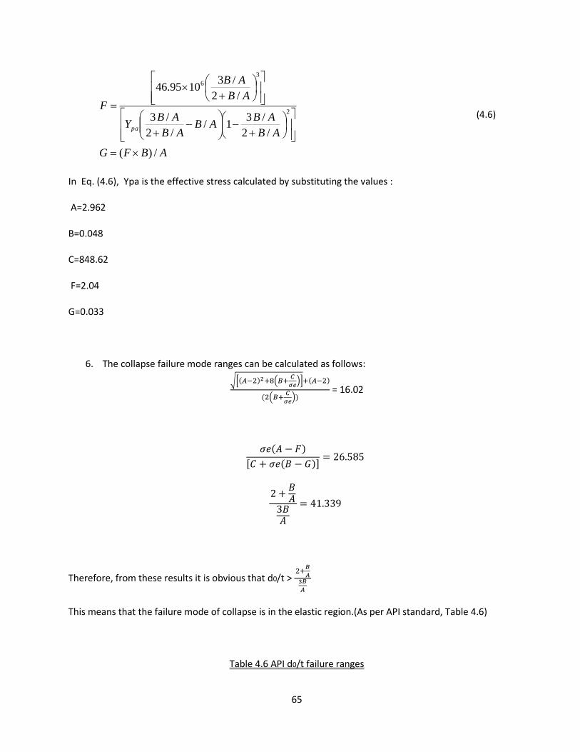
65

ABFG

AB

ABAB

AB

ABY

AB

AB

F

pa

/)(

/2

/31/

/2

/3

/2

/31095.46

2

3

6

(4.6)

In Eq. (4.6), Ypa is the effective stress calculated by substituting the values :

A=2.962

B=0.048

C=848.62

F=2.04

G=0.033

6. The collapse failure mode ranges can be calculated as follows:

√[(𝐴−2)2+8(𝐵+𝐶

𝜎𝑒)]+(𝐴−2)

(2(𝐵+𝐶

𝜎𝑒))

= 16.02

𝜎𝑒(𝐴 − 𝐹)

[𝐶 + 𝜎𝑒(𝐵 − 𝐺)]= 26.585

2 +𝐵𝐴

3𝐵𝐴

= 41.339

Therefore, from these results it is obvious that d0/t ˃ 2+

𝐵

𝐴3𝐵

𝐴

This means that the failure mode of collapse is in the elastic region.(As per API standard, Table 4.6)

Table 4.6 API d0/t failure ranges

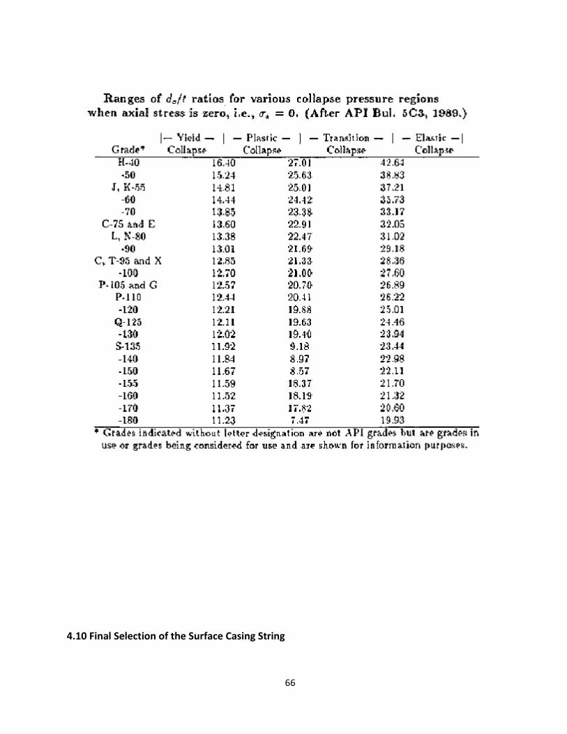
66

4.10 Final Selection of the Surface Casing String

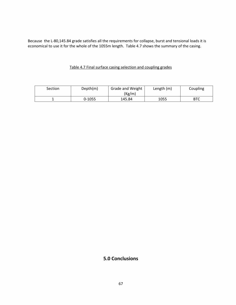
67

Because the L-80,145.84 grade satisfies all the requirements for collapse, burst and tensional loads it is economical to use it for the whole of the 1055m length. Table 4.7 shows the summary of the casing.

Table 4.7 Final surface casing selection and coupling grades

Section Depth(m) Grade and Weight (Kg/m)

Length (m) Coupling

1 0-1055 145.84 1055 BTC

5.0 Conclusions

68

5.1 Pore Pressure and Fracture Pressure Prediction

The purpose of this project was to develop a pore pressure and fracture pressure model for the Deep Panuke formation. The offset well data used consisted of eight wells in the Deep Panuke gas pool and nearby block. Analytical interpretation of field data was used to predict pore pressure and fracture pressure for the formation. An attempt was made to study and analyze several analytical methods. The data gathered from the well pressure logs give more accuracy compared to the correlations that exists. This was proven when the log data with real tested data were plotted on the same graph. From the data analyzed it is seen there is a slight transition zone when it enters the Abenaki-5 formation. The final conclusion from the analysis is that the formation is normally pressurized and has two pressures gradients one before the transition zone and one after the transition zone. The pore pressure predicted graph can be used as a reference for drillers in the Deep Panuke formation for future well drillings.

The Zamora method of pore pressure and fracture pressure prediction could provide another prediction if enough accurate field data of the drill bits and the bottom hole assembly (BHA) are recoded at each measured depth or vertical depth. Instead, an attempt was made to predict a pore pressure model using the existing average data for two wells. The predicted values were plotted with the pore pressure values from well logs. The variation was linear but did not agree with the log values. This may be due to the average values used from the well history reports. Due to the present lack of BHA data this is a possibility for future studies in the Deep Panuke area.

5.2 Casing Design

The most important parameter in determining the reliability and success of a casing design is the pore pressure. This means that the drilling engineer must consider all supporting data available to

69

determine the pore pressure confidence levels and ensure that all parameters impacting pore pressure predictions have been considered. For the Deep Panuke formation, detailed analysis of data obtained from various sources were carried out before finalizing a pore pressure and fracture pressure model for the formation.

When drilling to search for hydrocarbons in higher depths the number of casing strings and their sizes are increased. This will contribute to a higher percentage of the total cost in drilling. As a petroleum engineer the task was to design an economical casing which meets the safety requirements and appropriate regulations and standards. In the surface casing design for the new development well, collapse, burst, tension and biaxial design principles were studied to apply graphical methods for casing grade selection. Maximum load design principles and worst loading conditions were applied in designing the casing. When combinations of casing strings that satisfies all the requirements are selected, the most cost effective design will be achieved. In this case study the cheapest grade satisfies the whole length requirement. Further, when considering the safety of the design for burst criteria the worst case scenario was applied. That is, designing for a completely gas filled casing instead of a maximum kick margin.

When considering improvements to the surface casing design it was carried out according to the API and industry best practices. But, in some cases government regulations and local considerations may require that casing designs be carried out to standards exceeding those in the API and industry practices. If such requirements arise they can be added to the design criteria.

References:

1) Adam T.Bourgene Jr., Keith K.Milleim, Martin E.Chenvert, and F.S.Young Jr.(1986).Applied drilling

engineering.

70

2) Zaki Bassiouni(1994). Theory, Measurement and interpretation of well logs.

3) Bernt S.Adnoy(2010).Modern Well Design second edition

4) Tuna Eren ( Thesis real time optimization of drilling parameters during drilling operations)

5) Rahman,S.S.(1995).Casing Design Theory and Practice.

6) EnCana(2006). Deep Panuke project report-1.

7) EnCana Deep(2006). Panuke Project report-2 .

8) API Bul. 5C3, 5th Edition, July 1989. Bulletin on Formulas and Calculations for Casing, Tubing, Drill

Pipe and Line Pipe Properties. API Production Department.

9) API Bulletin 5C3, (1990).

10) Rabia, H., 1987. Fundamentals of Casing Design. Graham & Trotman, London,UK, pp. 1-2:]

11) Mississippi Canyon 252 No.1(Mcondo)Basis of Design Review

12) Sindre Stunes(2012).Methods of Pore Pressure Detection from Real-time Drilling Data.

13) Jincai Zhang(2011) Pore pressure prediction from well logs: Methods, modifications, and new

approaches. Article Earth-Science Reviews

14) Internet link.http://en.wikipedia.org/wiki/Well logging

Following Reference Documents are from Canada Nova Scotia Offshore Petroleum Board

15) CNSOPB Deep Panuke Development Plan Decision Report 2007

16) Report number-1222646_D390_WELL_HISTORY_VOLUMES_1_AND_2_PDF[1]

17) Report number-1222647_D390_WELL_HISTORY_VOLUME_3_PDF[1]

18) Report number-1222660_D390_PRESSURE_LOG_PDF[1]

19) Report number-1217369_D386_PRESSURE_LOG_PDF[1]

20) Report number-1217299_D386_WELL_HISTORY_-_VOLUME_1__PDF[1]

21) Report number-1223219_D400_PRESSURE_LOG_PDF[1]

22) Report number-1217986_D368_WELL_HISTORY_MANUAL_PANUKE_M-79_-_M-79A_-

_VOLUME_1_PDF[1]

23) Report number-1217998_D368_STRIP_LOG_PDF[1]

24) Report number-1024560_D354_FINAL_WELL_REPORT_VOLUME_1_PDF[1]

25) Report number-1223775_D362_PRESSURE_EVALUATION_LOG_PDF[1]

26) Report number-1223260_D360_WELL_HISTORY_PANUKE_PI1A_AND_PI1B_VOLUME_1_-

_PART_1_PDF[1]

27) Report number-1213607_D364_PRESSURE_EVALUATION_LOG_PDF[1]

28) Report number-1213566_D364_WELL_HISTORY_VOLUME_1_PDF[1]

29) Report number-1213567_D364_WELL_HISTORY_VOLUME_2_PDF[1]

Apendix-1

Deep Panuke Well Recaps

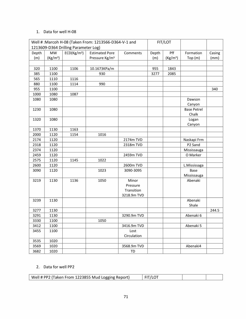
71

1. Data for well H-08

Well # :Marcoh H-08 (Taken From: 1213566-D364-V-1 and 1213609-D364 Drilling Parameter Log)

FIT/LOT

Depth (m)

MW (Kg/mᵌ)

ECD(Kg/mᶾ) Estimated Pore Pressure Kg/mᶾ

Comments Depth (m)

Pff (Kg/mᵌ)

Formation Top (m)

Casing (mm)

320 1100 1106 10.1673KPa/m 955 1843

385 1100 930 3277 2085

565 1110 1116

880 1100 1114 990

955 1100 340

1000 1080 1087

1080 1080 Dawson Canyon

1230 1080 Base Petrel Chalk

1320 1080 Logan Canyon

1370 1130 1163

2000 1120 1154 1016

2174 1120 2174m TVD Naskapi Frm

2318 1120 2318m TVD P2 Sand

2374 1120 Mississauga

2459 1120 2459m TVD O Marker

2575 1120 1145 1022

2600 1120 2600m TVD L.Mississaga

3090 1120 1023 3090-3095 Base Mississauga

3219 1130 1136 1050 Minor Pressure

Transition 3218.9m TVD

Abenaki

3239 1130 Abenaki Shale

3277 1130 244.5

3291 1130 3290.9m TVD Abenaki 6

3330 1100 1050

3412 1100 3416.9m TVD Abenaki 5

3455 1100 Lost Circulation

3535 1020

3569 1020 3568.9m TVD Abenaki4

3682 1020 TD

2. Data for well PP2

Well # PP2 (Taken From 1223855 Mud Logging Report) FIT/LOT

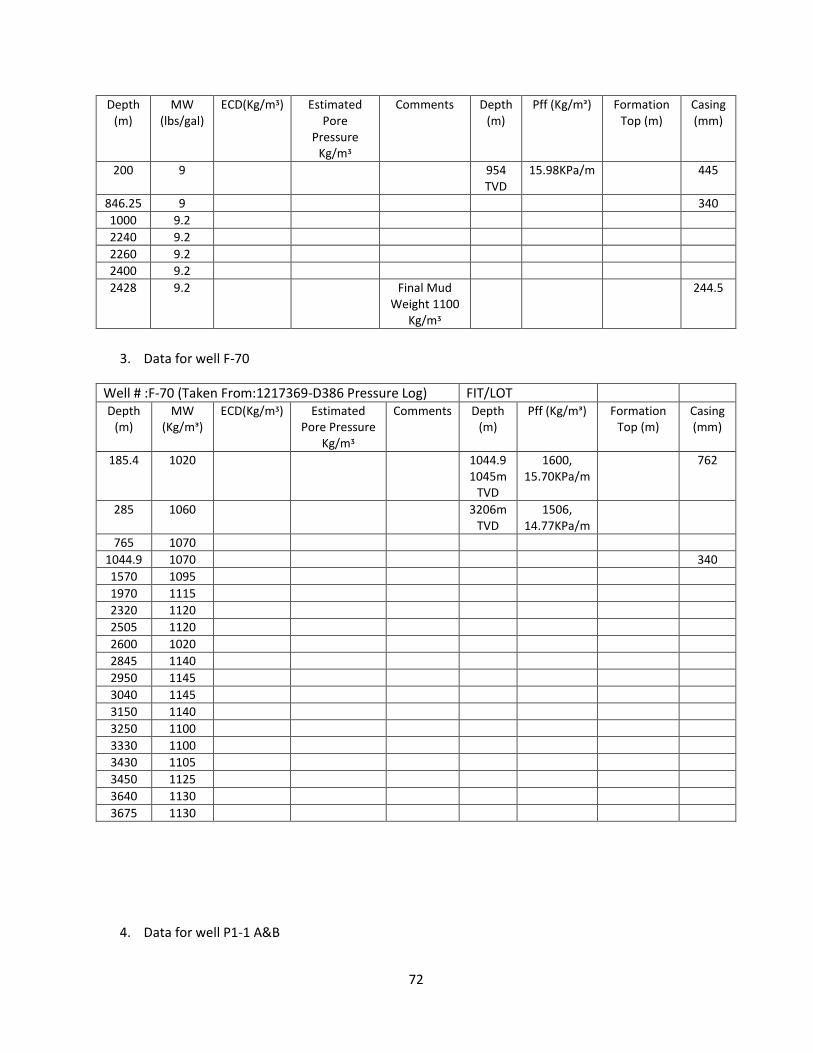
72

Depth (m)

MW (lbs/gal)

ECD(Kg/mᶾ) Estimated Pore

Pressure Kg/mᶾ

Comments Depth (m)

Pff (Kg/mᵌ) Formation Top (m)

Casing (mm)

200 9 954 TVD

15.98KPa/m 445

846.25 9 340

1000 9.2

2240 9.2

2260 9.2

2400 9.2

2428 9.2 Final Mud Weight 1100

Kg/mᶾ

244.5

3. Data for well F-70

Well # :F-70 (Taken From:1217369-D386 Pressure Log) FIT/LOT Depth

(m) MW

(Kg/mᵌ) ECD(Kg/mᶾ) Estimated

Pore Pressure Kg/mᶾ

Comments Depth (m)

Pff (Kg/mᵌ) Formation Top (m)

Casing (mm)

185.4 1020 1044.9 1045m

TVD

1600, 15.70KPa/m

762

285 1060 3206m TVD

1506, 14.77KPa/m

765 1070

1044.9 1070 340

1570 1095

1970 1115

2320 1120

2505 1120

2600 1020

2845 1140

2950 1145

3040 1145

3150 1140

3250 1100

3330 1100

3430 1105

3450 1125

3640 1130

3675 1130

4. Data for well P1-1 A&B

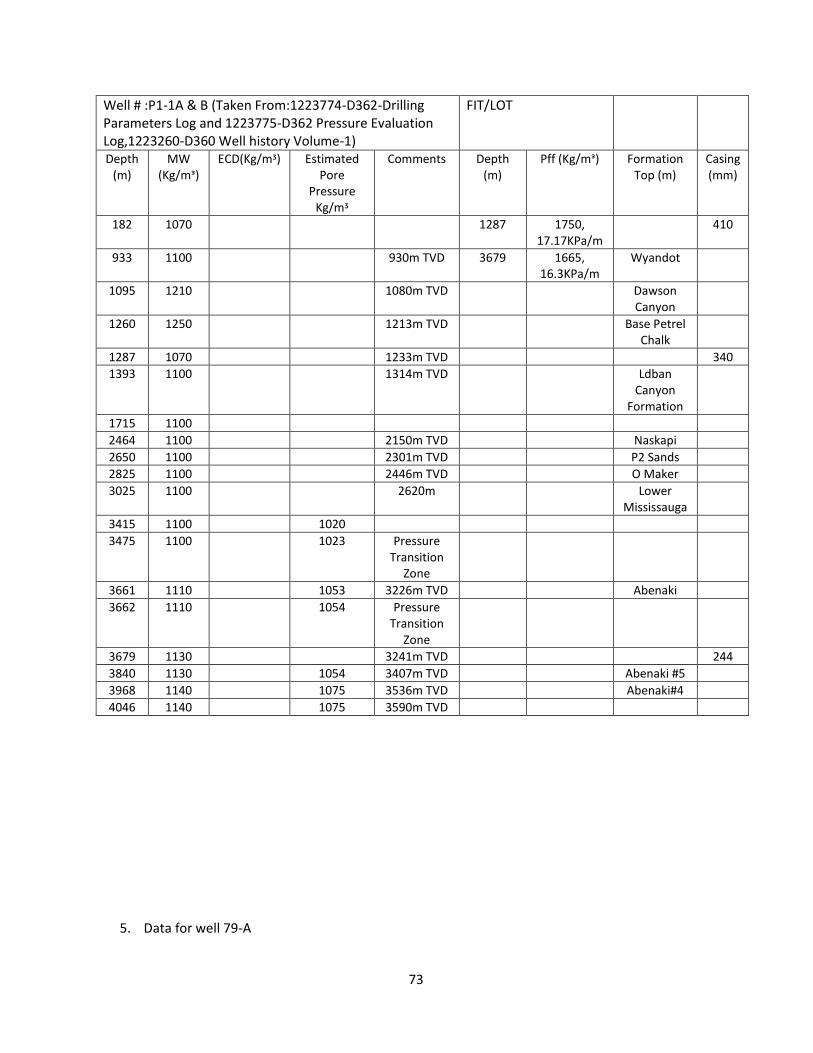
73

Well # :P1-1A & B (Taken From:1223774-D362-Drilling Parameters Log and 1223775-D362 Pressure Evaluation Log,1223260-D360 Well history Volume-1)

FIT/LOT

Depth (m)

MW (Kg/mᵌ)

ECD(Kg/mᶾ) Estimated Pore

Pressure Kg/mᶾ

Comments Depth (m)

Pff (Kg/mᵌ) Formation Top (m)

Casing (mm)

182 1070 1287 1750, 17.17KPa/m

410

933 1100 930m TVD 3679 1665, 16.3KPa/m

Wyandot

1095 1210 1080m TVD Dawson Canyon

1260 1250 1213m TVD Base Petrel Chalk

1287 1070 1233m TVD 340

1393 1100 1314m TVD Ldban Canyon

Formation

1715 1100

2464 1100 2150m TVD Naskapi

2650 1100 2301m TVD P2 Sands

2825 1100 2446m TVD O Maker

3025 1100 2620m Lower Mississauga

3415 1100 1020

3475 1100 1023 Pressure Transition

Zone

3661 1110 1053 3226m TVD Abenaki

3662 1110 1054 Pressure Transition

Zone

3679 1130 3241m TVD 244

3840 1130 1054 3407m TVD Abenaki #5

3968 1140 1075 3536m TVD Abenaki#4

4046 1140 1075 3590m TVD

5. Data for well 79-A

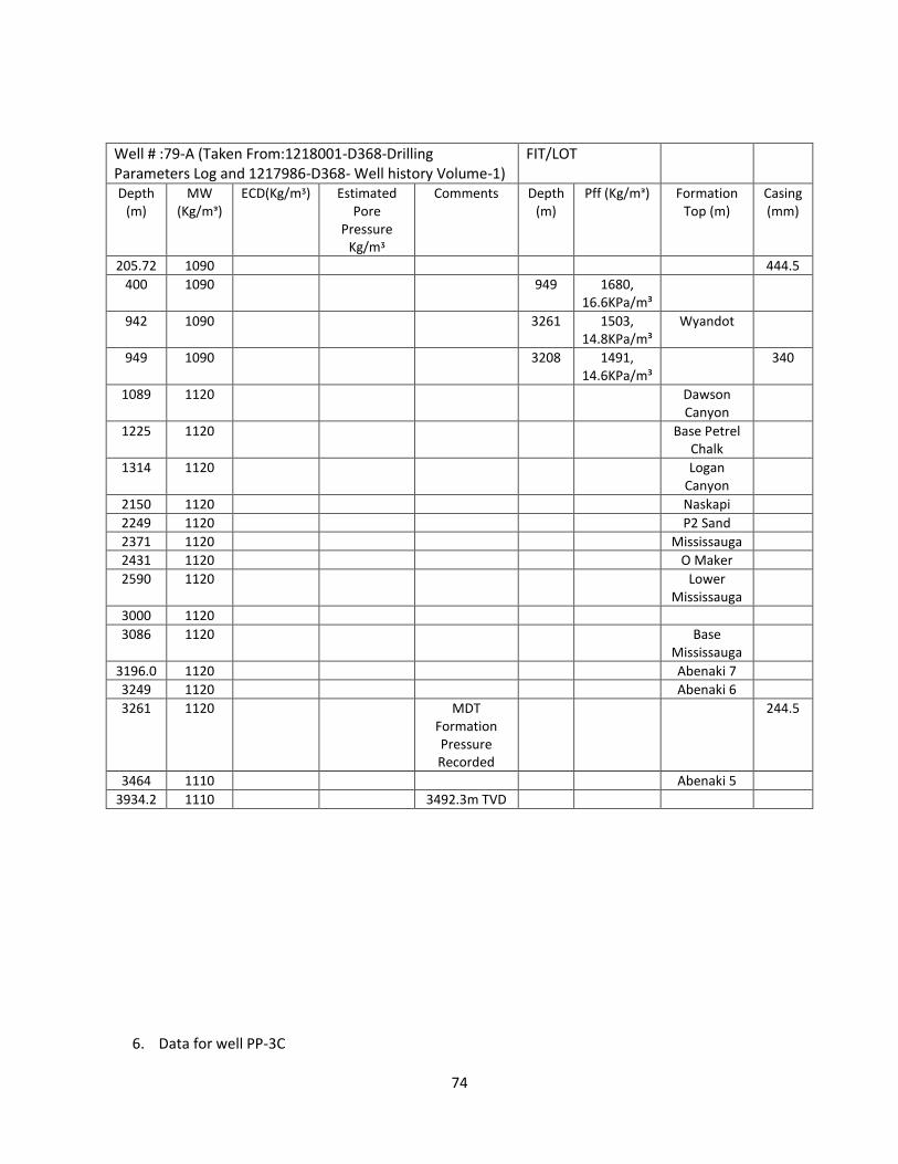
74

Well # :79-A (Taken From:1218001-D368-Drilling Parameters Log and 1217986-D368- Well history Volume-1)

FIT/LOT

Depth (m)

MW (Kg/mᵌ)

ECD(Kg/mᶾ) Estimated Pore

Pressure Kg/mᶾ

Comments Depth (m)

Pff (Kg/mᵌ) Formation Top (m)

Casing (mm)

205.72 1090 444.5

400 1090 949 1680, 16.6KPa/m³

942 1090 3261 1503, 14.8KPa/m³

Wyandot

949 1090 3208 1491, 14.6KPa/m³

340

1089 1120 Dawson Canyon

1225 1120 Base Petrel Chalk

1314 1120 Logan Canyon

2150 1120 Naskapi

2249 1120 P2 Sand

2371 1120 Mississauga

2431 1120 O Maker

2590 1120 Lower Mississauga

3000 1120

3086 1120 Base Mississauga

3196.0 1120 Abenaki 7

3249 1120 Abenaki 6

3261 1120 MDT Formation Pressure Recorded

244.5

3464 1110 Abenaki 5

3934.2 1110 3492.3m TVD

6. Data for well PP-3C

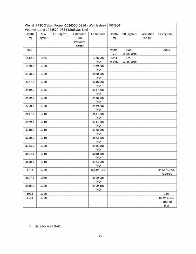
75

Well # :PP3C (Taken From- -1024560-D354 - Well history Volume-1 and 1024570-D354-Mud-Gas Log)

FIT/LOT

Depth (m)

MW (Kg/mᵌ)

ECD(Kg/mᶾ) Estimated Pore

Pressure Kg/mᶾ

Comments Depth (m)

Pff (Kg/mᵌ) Formation Top (m)

Casing (mm)

964 958m TVD

1900, 18.6KPa/m

298.5

1812.5 1075 1776.9m TVD

3253m TVD

1250, 12.3KPa/m

1980.8 1100 1939.6m TVD

2128.5 1100 2080.2m TVD

2277.2 1150 2216.8m TVD

2419.0 1155 2337.8m TVD

2559.5 1150 2448.6m TVD

2700.4 1150 2549.6m TVD

2837.7 1110 2831.8m TVD

2979.3 1110 2711.3m TVD

3110.9 1110 2788.4m TVD

3250.9 1110 2872.4m TVD

3363.9 1100 2945.3m TVD

3504.5 1110 3050.2m TVD

3650.5 1110 3173.9m TVD

3742 1120 3253m TVD 244.5*177.8-Tapered

3807.6 1030 3309.9m TVD

3915.0 1100 3409.1m TVD

3928 1120 156

4163 1120 88.9*114.3 Tapered

liner

7. Data for well D-41

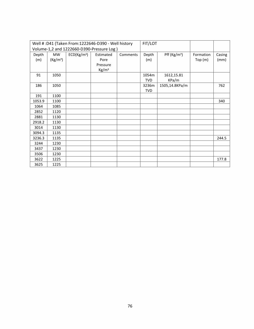
76

Well # :D41 (Taken From:1222646-D390 - Well history Volume-1,2 and 1222660-D390-Pressure Log )

FIT/LOT

Depth (m)

MW (Kg/mᵌ)

ECD(Kg/mᶾ) Estimated Pore

Pressure Kg/mᶾ

Comments Depth (m)

Pff (Kg/mᵌ) Formation Top (m)

Casing (mm)

91 1050 1054m TVD

1612,15.81 KPa/m

186 1050 3236m TVD

1505,14.8KPa/m 762

191 1100

1053.9 1100 340

1064 1085

2852 1120

2881 1130

2918.2 1130

3014 1130

3094.3 1135

3236.3 1135 244.5

3244 1230

3437 1230

3506 1230

3622 1225 177.8

3625 1225

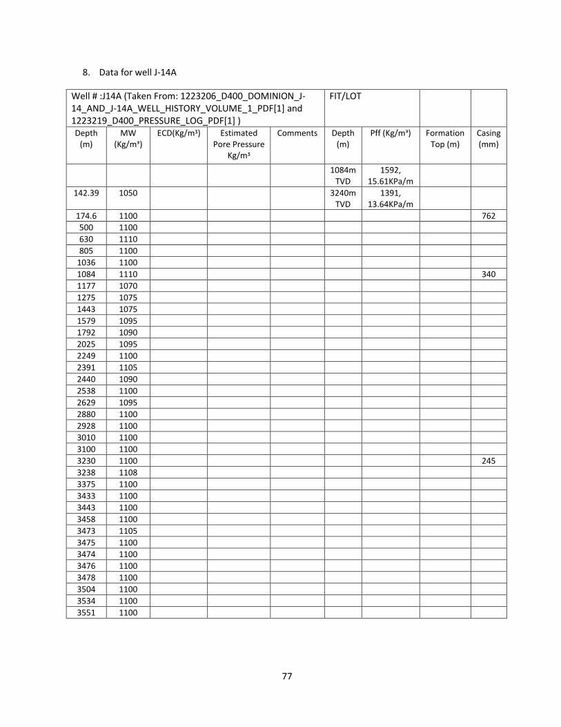
77

8. Data for well J-14A

Well # :J14A (Taken From: 1223206_D400_DOMINION_J-14_AND_J-14A_WELL_HISTORY_VOLUME_1_PDF[1] and 1223219_D400_PRESSURE_LOG_PDF[1] )

FIT/LOT

Depth (m)

MW (Kg/mᵌ)

ECD(Kg/mᶾ) Estimated Pore Pressure

Kg/mᶾ

Comments Depth (m)

Pff (Kg/mᵌ) Formation Top (m)

Casing (mm)

1084m TVD

1592, 15.61KPa/m

142.39 1050 3240m TVD

1391, 13.64KPa/m

174.6 1100 762

500 1100

630 1110

805 1100

1036 1100

1084 1110 340

1177 1070

1275 1075

1443 1075

1579 1095

1792 1090

2025 1095

2249 1100

2391 1105

2440 1090

2538 1100

2629 1095

2880 1100

2928 1100

3010 1100

3100 1100

3230 1100 245

3238 1108

3375 1100

3433 1100

3443 1100

3458 1100

3473 1105

3475 1100

3474 1100

3476 1100

3478 1100

3504 1100

3534 1100

3551 1100

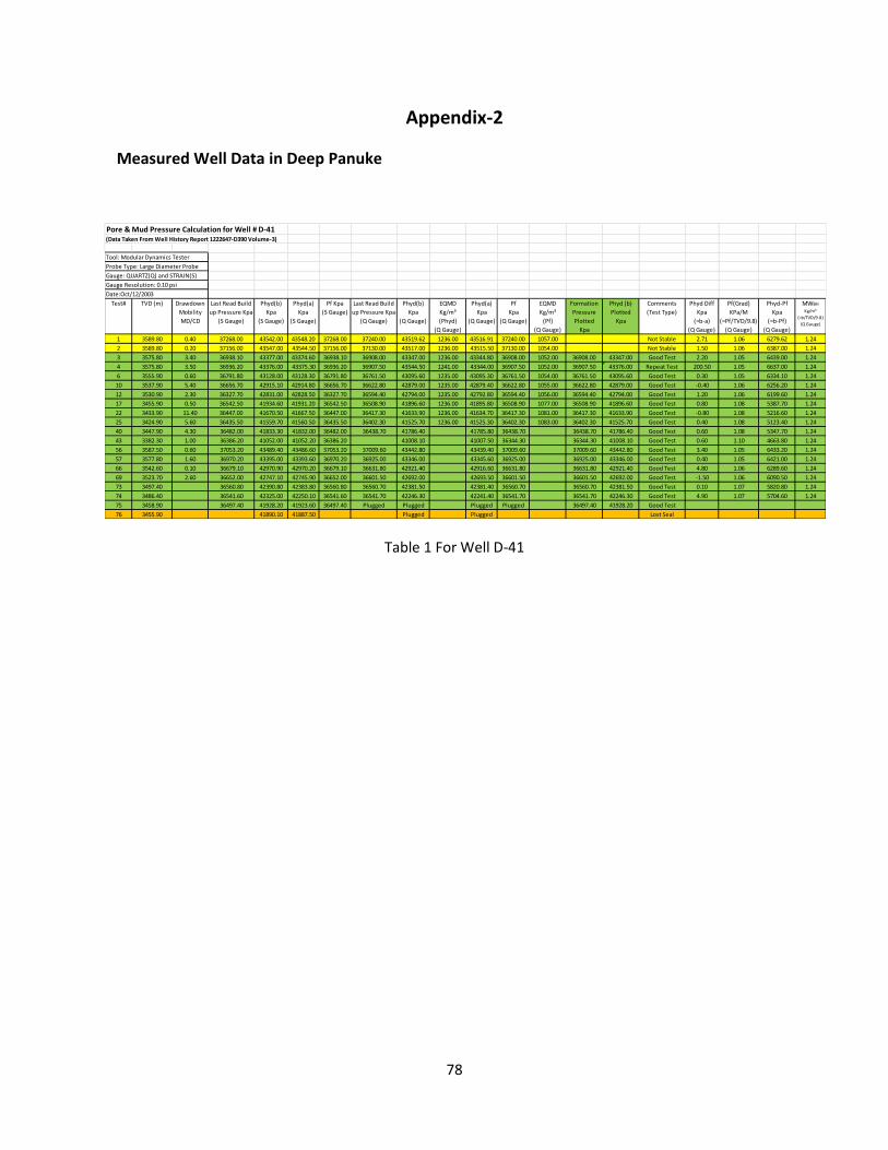
78

Appendix-2

Measured Well Data in Deep Panuke

Table 1 For Well D-41

Pore & Mud Pressure Calculation for Well # D-41(Data Taken From Well History Report 1222647-D390 Volume-3)

Test# TVD (m) Drawdown

Mobility

MD/CD

Last Read Build

up Pressure Kpa

(S Gauge)

Phyd(b)

Kpa

(S Gauge)

Phyd(a)

Kpa

(S Gauge)

Pf Kpa

(S Gauge)

Last Read Build

up Pressure Kpa

(Q Gauge)

Phyd(b)

Kpa

(Q Gauge)

EQMD

Kg/m³

(Phyd)

(Q Gauge)

Phyd(a)

Kpa

(Q Gauge)

Pf

Kpa

(Q Gauge)

EQMD

Kg/m³

(Pf)

(Q Gauge)

Formation

Pressure

Plotted

Kpa

Phyd (b)

Plotted

Kpa

Comments

(Test Type)

Phyd Diff

Kpa

(=b-a)

(Q Gauge)

Pf(Grad)

KPa/M

(=Pf/TVD/9.8)

(Q Gauge)

Phyd-Pf

Kpa

(=b-Pf)

(Q Gauge)

MWBH

Kg/m³

(=b/TVD/9.8)

(Q Gauge)

1 3589.80 0.40 37268.00 43542.00 43548.20 37268.00 37240.00 43519.62 1236.00 43516.91 37240.00 1057.00 Not Stable 2.71 1.06 6279.62 1.24

2 3589.80 0.20 37156.00 43547.00 43544.50 37156.00 37130.00 43517.00 1236.00 43515.50 37130.00 1054.00 Not Stable 1.50 1.06 6387.00 1.24

3 3575.80 3.40 36938.10 43377.00 43374.60 36938.10 36908.00 43347.00 1236.00 43344.80 36908.00 1052.00 36908.00 43347.00 Good Test 2.20 1.05 6439.00 1.24

4 3575.80 3.50 36936.20 43376.00 43375.30 36936.20 36907.50 43544.50 1241.00 43344.00 36907.50 1052.00 36907.50 43376.00 Repeat Test 200.50 1.05 6637.00 1.24

6 3555.90 0.60 36791.80 43128.00 43128.30 36791.80 36761.50 43095.60 1235.00 43095.30 36761.50 1054.00 36761.50 43095.60 Good Test 0.30 1.05 6334.10 1.24

10 3537.90 5.40 36656.70 42915.10 42914.80 36656.70 36622.80 42879.00 1235.00 42879.40 36622.80 1055.00 36622.80 42879.00 Good Test -0.40 1.06 6256.20 1.24

12 3530.90 2.30 36327.70 42831.00 42828.50 36327.70 36594.40 42794.00 1235.00 42792.80 36594.40 1056.00 36594.40 42794.00 Good Test 1.20 1.06 6199.60 1.24

17 3455.90 0.50 36542.50 41934.60 41931.20 36542.50 36508.90 41896.60 1236.00 41895.80 36508.90 1077.00 36508.90 41896.60 Good Test 0.80 1.08 5387.70 1.24

22 3433.90 11.40 36447.00 41670.50 41667.50 36447.00 36417.30 41633.90 1236.00 41634.70 36417.30 1081.00 36417.30 41633.90 Good Test -0.80 1.08 5216.60 1.24

25 3424.90 5.60 36435.50 41559.70 41560.50 36435.50 36402.30 41525.70 1236.00 41525.30 36402.30 1083.00 36402.30 41525.70 Good Test 0.40 1.08 5123.40 1.24

40 3447.90 4.30 36482.00 41833.30 41832.00 36482.00 36438.70 41786.40 41785.80 36438.70 36438.70 41786.40 Good Test 0.60 1.08 5347.70 1.24

43 3382.30 1.00 36386.20 41052.00 41052.20 36386.20 41008.10 41007.50 36344.30 36344.30 41008.10 Good Test 0.60 1.10 4663.80 1.24

56 3587.50 0.60 37053.20 43489.40 43486.60 37053.20 37009.60 43442.80 43439.40 37009.60 37009.60 43442.80 Good Test 3.40 1.05 6433.20 1.24

57 3577.80 1.60 36970.20 43395.00 43393.60 36970.20 36925.00 43346.00 43345.60 36925.00 36925.00 43346.00 Good Test 0.40 1.05 6421.00 1.24

66 3542.60 0.10 36679.10 42970.90 42970.20 36679.10 36631.80 42921.40 42916.60 36631.80 36631.80 42921.40 Good Test 4.80 1.06 6289.60 1.24

69 3523.70 2.60 36652.00 42747.10 42745.90 36652.00 36601.50 42692.00 42693.50 36601.50 36601.50 42692.00 Good Test -1.50 1.06 6090.50 1.24

73 3497.40 36560.80 42390.80 42383.80 36560.80 36560.70 42381.50 42381.40 36560.70 36560.70 42381.50 Good Test 0.10 1.07 5820.80 1.24

74 3486.40 36541.60 42325.00 42250.10 36541.60 36541.70 42246.30 42241.40 36541.70 36541.70 42246.30 Good Test 4.90 1.07 5704.60 1.24

75 3458.90 36497.40 41928.20 41923.60 36497.40 Plugged Plugged Plugged Plugged 36497.40 41928.20 Good Test

76 3455.90 41890.10 41887.50 Plugged Plugged Lost Seal

Tool: Modular Dynamics Tester

Probe Type: Large Diameter Probe

Gauge: QUARTZ(Q) and STRAIN(S)

Gauge Resolution: 0.10 psi

Date:Oct/12/2003

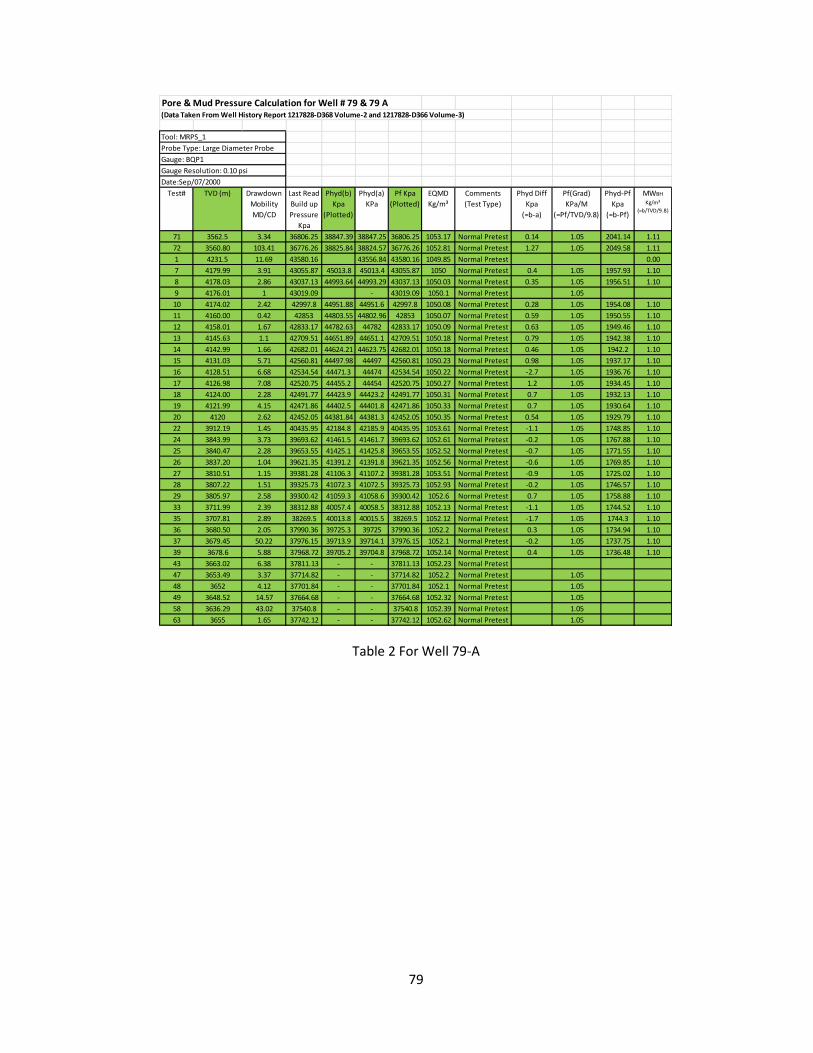
79

Table 2 For Well 79-A

Pore & Mud Pressure Calculation for Well # 79 & 79 A(Data Taken From Well History Report 1217828-D368 Volume-2 and 1217828-D366 Volume-3)

Test# TVD (m) Drawdown

Mobility

MD/CD

Last Read

Build up

Pressure

Kpa

Phyd(b)

Kpa

(Plotted)

Phyd(a)

KPa

Pf Kpa

(Plotted)

EQMD

Kg/m³

Comments

(Test Type)

Phyd Diff

Kpa

(=b-a)

Pf(Grad)

KPa/M

(=Pf/TVD/9.8)

Phyd-Pf

Kpa

(=b-Pf)

MWBH

Kg/m³

(=b/TVD/9.8)

71 3562.5 3.34 36806.25 38847.39 38847.25 36806.25 1053.17 Normal Pretest 0.14 1.05 2041.14 1.11

72 3560.80 103.41 36776.26 38825.84 38824.57 36776.26 1052.81 Normal Pretest 1.27 1.05 2049.58 1.11

1 4231.5 11.69 43580.16 43556.84 43580.16 1049.85 Normal Pretest 0.00

7 4179.99 3.91 43055.87 45013.8 45013.4 43055.87 1050 Normal Pretest 0.4 1.05 1957.93 1.10

8 4178.03 2.86 43037.13 44993.64 44993.29 43037.13 1050.03 Normal Pretest 0.35 1.05 1956.51 1.10

9 4176.01 1 43019.09 - 43019.09 1050.1 Normal Pretest 1.05

10 4174.02 2.42 42997.8 44951.88 44951.6 42997.8 1050.08 Normal Pretest 0.28 1.05 1954.08 1.10

11 4160.00 0.42 42853 44803.55 44802.96 42853 1050.07 Normal Pretest 0.59 1.05 1950.55 1.10

12 4158.01 1.67 42833.17 44782.63 44782 42833.17 1050.09 Normal Pretest 0.63 1.05 1949.46 1.10

13 4145.63 1.1 42709.51 44651.89 44651.1 42709.51 1050.18 Normal Pretest 0.79 1.05 1942.38 1.10

14 4142.99 1.66 42682.01 44624.21 44623.75 42682.01 1050.18 Normal Pretest 0.46 1.05 1942.2 1.10

15 4131.03 5.71 42560.81 44497.98 44497 42560.81 1050.23 Normal Pretest 0.98 1.05 1937.17 1.10

16 4128.51 6.68 42534.54 44471.3 44474 42534.54 1050.22 Normal Pretest -2.7 1.05 1936.76 1.10

17 4126.98 7.08 42520.75 44455.2 44454 42520.75 1050.27 Normal Pretest 1.2 1.05 1934.45 1.10

18 4124.00 2.28 42491.77 44423.9 44423.2 42491.77 1050.31 Normal Pretest 0.7 1.05 1932.13 1.10

19 4121.99 4.15 42471.86 44402.5 44401.8 42471.86 1050.33 Normal Pretest 0.7 1.05 1930.64 1.10

20 4120 2.62 42452.05 44381.84 44381.3 42452.05 1050.35 Normal Pretest 0.54 1.05 1929.79 1.10

22 3912.19 1.45 40435.95 42184.8 42185.9 40435.95 1053.61 Normal Pretest -1.1 1.05 1748.85 1.10

24 3843.99 3.73 39693.62 41461.5 41461.7 39693.62 1052.61 Normal Pretest -0.2 1.05 1767.88 1.10

25 3840.47 2.28 39653.55 41425.1 41425.8 39653.55 1052.52 Normal Pretest -0.7 1.05 1771.55 1.10

26 3837.20 1.04 39621.35 41391.2 41391.8 39621.35 1052.56 Normal Pretest -0.6 1.05 1769.85 1.10

27 3810.51 1.15 39381.28 41106.3 41107.2 39381.28 1053.51 Normal Pretest -0.9 1.05 1725.02 1.10

28 3807.22 1.51 39325.73 41072.3 41072.5 39325.73 1052.93 Normal Pretest -0.2 1.05 1746.57 1.10

29 3805.97 2.58 39300.42 41059.3 41058.6 39300.42 1052.6 Normal Pretest 0.7 1.05 1758.88 1.10

33 3711.99 2.39 38312.88 40057.4 40058.5 38312.88 1052.13 Normal Pretest -1.1 1.05 1744.52 1.10

35 3707.81 2.89 38269.5 40013.8 40015.5 38269.5 1052.12 Normal Pretest -1.7 1.05 1744.3 1.10

36 3680.50 2.05 37990.36 39725.3 39725 37990.36 1052.2 Normal Pretest 0.3 1.05 1734.94 1.10

37 3679.45 50.22 37976.15 39713.9 39714.1 37976.15 1052.1 Normal Pretest -0.2 1.05 1737.75 1.10

39 3678.6 5.88 37968.72 39705.2 39704.8 37968.72 1052.14 Normal Pretest 0.4 1.05 1736.48 1.10

43 3663.02 6.38 37811.13 - - 37811.13 1052.23 Normal Pretest

47 3653.49 3.37 37714.82 - - 37714.82 1052.2 Normal Pretest 1.05

48 3652 4.12 37701.84 - - 37701.84 1052.1 Normal Pretest 1.05

49 3648.52 14.57 37664.68 - - 37664.68 1052.32 Normal Pretest 1.05

58 3636.29 43.02 37540.8 - - 37540.8 1052.39 Normal Pretest 1.05

63 3655 1.65 37742.12 - - 37742.12 1052.62 Normal Pretest 1.05

Tool: MRPS_1

Probe Type: Large Diameter Probe

Gauge: BQP1

Gauge Resolution: 0.10 psi

Date:Sep/07/2000

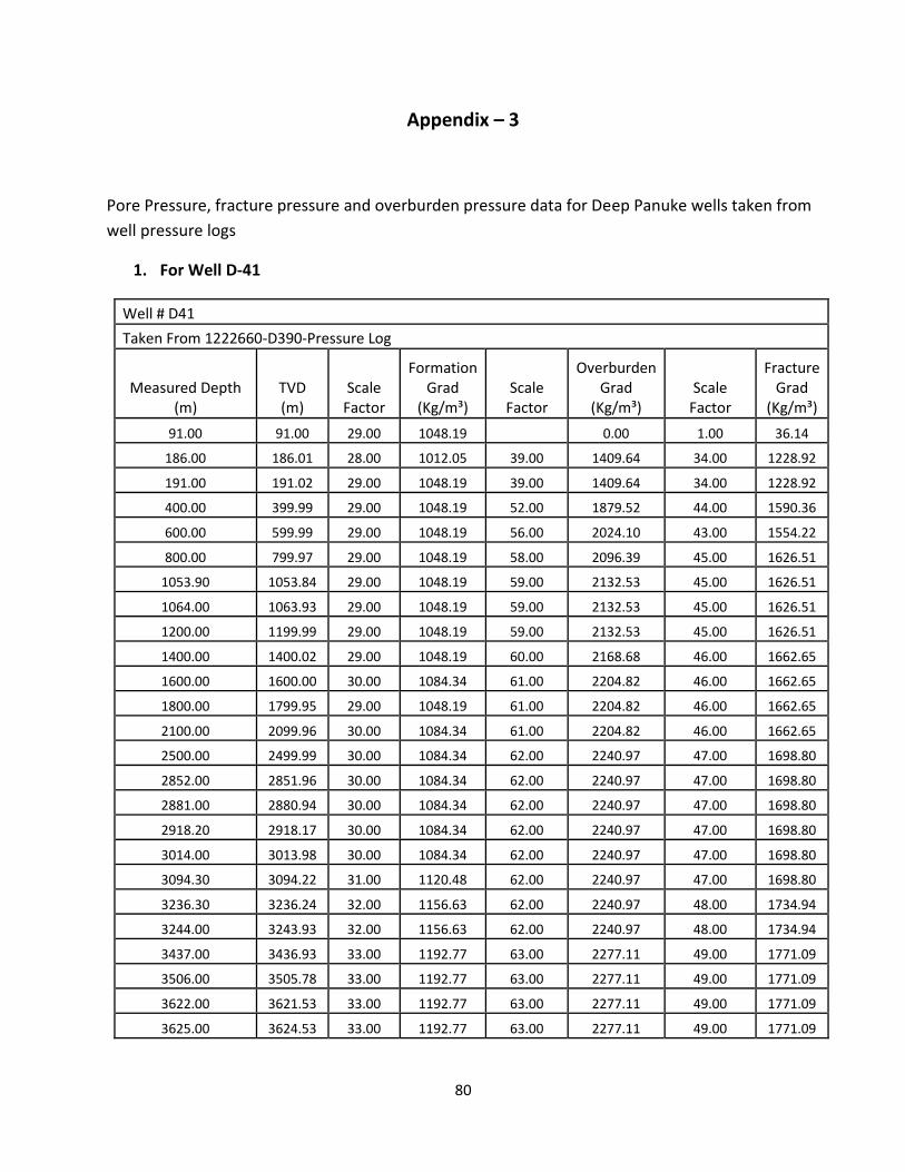
80

Appendix – 3

Pore Pressure, fracture pressure and overburden pressure data for Deep Panuke wells taken from

well pressure logs

1. For Well D-41

Well # D41

Taken From 1222660-D390-Pressure Log

Measured Depth (m)

TVD (m)

Scale Factor

Formation Grad

(Kg/m³) Scale

Factor

Overburden Grad

(Kg/m³) Scale

Factor

Fracture Grad

(Kg/m³)

91.00 91.00 29.00 1048.19 0.00 1.00 36.14

186.00 186.01 28.00 1012.05 39.00 1409.64 34.00 1228.92

191.00 191.02 29.00 1048.19 39.00 1409.64 34.00 1228.92

400.00 399.99 29.00 1048.19 52.00 1879.52 44.00 1590.36

600.00 599.99 29.00 1048.19 56.00 2024.10 43.00 1554.22

800.00 799.97 29.00 1048.19 58.00 2096.39 45.00 1626.51

1053.90 1053.84 29.00 1048.19 59.00 2132.53 45.00 1626.51

1064.00 1063.93 29.00 1048.19 59.00 2132.53 45.00 1626.51

1200.00 1199.99 29.00 1048.19 59.00 2132.53 45.00 1626.51

1400.00 1400.02 29.00 1048.19 60.00 2168.68 46.00 1662.65

1600.00 1600.00 30.00 1084.34 61.00 2204.82 46.00 1662.65

1800.00 1799.95 29.00 1048.19 61.00 2204.82 46.00 1662.65

2100.00 2099.96 30.00 1084.34 61.00 2204.82 46.00 1662.65

2500.00 2499.99 30.00 1084.34 62.00 2240.97 47.00 1698.80

2852.00 2851.96 30.00 1084.34 62.00 2240.97 47.00 1698.80

2881.00 2880.94 30.00 1084.34 62.00 2240.97 47.00 1698.80

2918.20 2918.17 30.00 1084.34 62.00 2240.97 47.00 1698.80

3014.00 3013.98 30.00 1084.34 62.00 2240.97 47.00 1698.80

3094.30 3094.22 31.00 1120.48 62.00 2240.97 47.00 1698.80

3236.30 3236.24 32.00 1156.63 62.00 2240.97 48.00 1734.94

3244.00 3243.93 32.00 1156.63 62.00 2240.97 48.00 1734.94

3437.00 3436.93 33.00 1192.77 63.00 2277.11 49.00 1771.09

3506.00 3505.78 33.00 1192.77 63.00 2277.11 49.00 1771.09

3622.00 3621.53 33.00 1192.77 63.00 2277.11 49.00 1771.09

3625.00 3624.53 33.00 1192.77 63.00 2277.11 49.00 1771.09

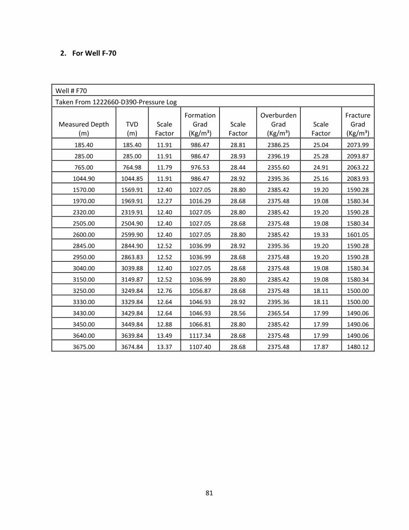
81

2. For Well F-70

Well # F70

Taken From 1222660-D390-Pressure Log

Measured Depth (m)

TVD (m)

Scale Factor

Formation Grad

(Kg/m³) Scale

Factor

Overburden Grad

(Kg/m³) Scale

Factor

Fracture Grad

(Kg/m³)

185.40 185.40 11.91 986.47 28.81 2386.25 25.04 2073.99

285.00 285.00 11.91 986.47 28.93 2396.19 25.28 2093.87

765.00 764.98 11.79 976.53 28.44 2355.60 24.91 2063.22

1044.90 1044.85 11.91 986.47 28.92 2395.36 25.16 2083.93

1570.00 1569.91 12.40 1027.05 28.80 2385.42 19.20 1590.28

1970.00 1969.91 12.27 1016.29 28.68 2375.48 19.08 1580.34

2320.00 2319.91 12.40 1027.05 28.80 2385.42 19.20 1590.28

2505.00 2504.90 12.40 1027.05 28.68 2375.48 19.08 1580.34

2600.00 2599.90 12.40 1027.05 28.80 2385.42 19.33 1601.05

2845.00 2844.90 12.52 1036.99 28.92 2395.36 19.20 1590.28

2950.00 2863.83 12.52 1036.99 28.68 2375.48 19.20 1590.28

3040.00 3039.88 12.40 1027.05 28.68 2375.48 19.08 1580.34

3150.00 3149.87 12.52 1036.99 28.80 2385.42 19.08 1580.34

3250.00 3249.84 12.76 1056.87 28.68 2375.48 18.11 1500.00

3330.00 3329.84 12.64 1046.93 28.92 2395.36 18.11 1500.00

3430.00 3429.84 12.64 1046.93 28.56 2365.54 17.99 1490.06

3450.00 3449.84 12.88 1066.81 28.80 2385.42 17.99 1490.06

3640.00 3639.84 13.49 1117.34 28.68 2375.48 17.99 1490.06

3675.00 3674.84 13.37 1107.40 28.68 2375.48 17.87 1480.12

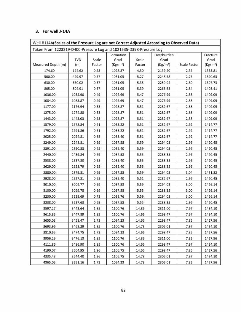
82

3. For well J-14A

Well # J14A(Scales of the Pressure Log are not Correct Adjusted According to Observed Data)

Taken From 1223219-D400-Pressure Log and 1021535-D398-Pressure Log

Measured Depth (m) TVD (m)

Scale Factor

Formation Grad

(Kg/m³) Scale

Factor

Overburden Grad

(Kg/m³) Scale Factor

Fracture Grad

(Kg/m³)

174.60 174.62 0.53 1028.87 4.50 2139.20 2.35 1333.81

500.00 499.97 0.57 1031.05 5.27 2248.58 2.75 1390.63

630.00 630.02 0.57 1031.05 5.35 2259.94 2.80 1397.73

805.00 804.91 0.57 1031.05 5.39 2265.63 2.84 1403.41

1036.00 1035.90 0.49 1026.69 5.47 2276.99 2.88 1409.09

1084.00 1083.87 0.49 1026.69 5.47 2276.99 2.88 1409.09

1177.00 1176.94 0.53 1028.87 5.51 2282.67 2.88 1409.09

1275.00 1274.88 0.53 1028.87 5.51 2282.67 2.88 1409.09

1443.00 1443.03 0.53 1028.87 5.51 2282.67 2.88 1409.09

1579.00 1578.84 0.61 1033.22 5.51 2282.67 2.92 1414.77

1792.00 1791.86 0.61 1033.22 5.51 2282.67 2.92 1414.77

2025.00 2024.81 0.65 1035.40 5.51 2282.67 2.92 1414.77

2249.00 2248.81 0.69 1037.58 5.59 2294.03 2.96 1420.45

2391.00 2390.83 0.65 1035.40 5.59 2294.03 2.96 1420.45

2440.00 2439.84 0.69 1037.58 5.55 2288.35 2.96 1420.45

2538.00 2537.80 0.65 1035.40 5.55 2288.35 2.96 1420.45

2629.00 2628.79 0.65 1035.40 5.55 2288.35 2.96 1420.45

2880.00 2879.81 0.69 1037.58 5.59 2294.03 3.04 1431.82

2928.00 2927.81 0.65 1035.40 5.51 2282.67 2.96 1420.45

3010.00 3009.77 0.69 1037.58 5.59 2294.03 3.00 1426.14

3100.00 3099.78 0.69 1037.58 5.55 2288.35 3.00 1426.14

3230.00 3229.69 0.73 1039.76 5.59 2294.03 3.00 1426.14

3238.00 3237.63 0.69 1037.58 5.55 2288.35 2.96 1420.45

3597.27 3443.64 1.85 1100.76 14.89 2311.00 7.97 1434.10

3615.85 3447.89 1.85 1100.76 14.66 2298.47 7.97 1434.10

3655.03 3458.47 1.73 1094.23 14.66 2298.47 7.85 1427.56

3693.96 3468.29 1.85 1100.76 14.78 2305.01 7.97 1434.10

3810.65 3474.75 1.73 1094.23 14.66 2298.47 7.85 1427.56

3956.29 3476.13 1.85 1100.76 14.89 2311.00 7.85 1427.56

4111.86 3486.90 1.85 1100.76 14.66 2298.47 7.97 1434.10

4190.07 3504.95 1.96 1106.75 14.66 2298.47 7.85 1427.56

4335.43 3544.40 1.96 1106.75 14.78 2305.01 7.97 1434.10

4365.05 3551.16 1.73 1094.23 14.78 2305.01 7.85 1427.56

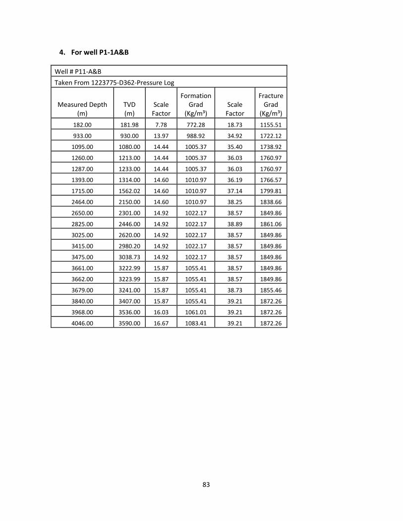
83

4. For well P1-1A&B

Well # P11-A&B

Taken From 1223775-D362-Pressure Log

Measured Depth (m)

TVD (m)

Scale Factor

Formation Grad

(Kg/m³) Scale

Factor

Fracture Grad

(Kg/m³)

182.00 181.98 7.78 772.28 18.73 1155.51

933.00 930.00 13.97 988.92 34.92 1722.12

1095.00 1080.00 14.44 1005.37 35.40 1738.92

1260.00 1213.00 14.44 1005.37 36.03 1760.97

1287.00 1233.00 14.44 1005.37 36.03 1760.97

1393.00 1314.00 14.60 1010.97 36.19 1766.57

1715.00 1562.02 14.60 1010.97 37.14 1799.81

2464.00 2150.00 14.60 1010.97 38.25 1838.66

2650.00 2301.00 14.92 1022.17 38.57 1849.86

2825.00 2446.00 14.92 1022.17 38.89 1861.06

3025.00 2620.00 14.92 1022.17 38.57 1849.86

3415.00 2980.20 14.92 1022.17 38.57 1849.86

3475.00 3038.73 14.92 1022.17 38.57 1849.86

3661.00 3222.99 15.87 1055.41 38.57 1849.86

3662.00 3223.99 15.87 1055.41 38.57 1849.86

3679.00 3241.00 15.87 1055.41 38.73 1855.46

3840.00 3407.00 15.87 1055.41 39.21 1872.26

3968.00 3536.00 16.03 1061.01 39.21 1872.26

4046.00 3590.00 16.67 1083.41 39.21 1872.26

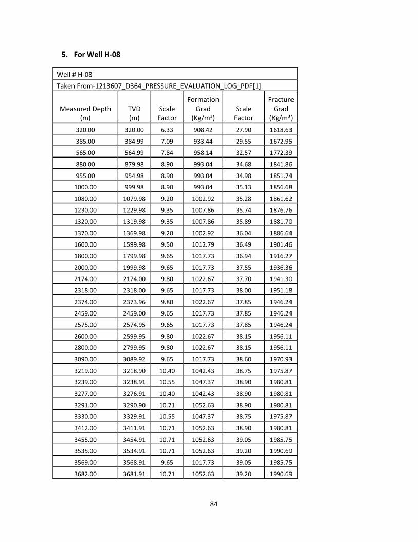
84

5. For Well H-08

Well # H-08

Taken From-1213607_D364_PRESSURE_EVALUATION_LOG_PDF[1]

Measured Depth (m)

TVD (m)

Scale Factor

Formation Grad

(Kg/m³) Scale

Factor

Fracture Grad

(Kg/m³)

320.00 320.00 6.33 908.42 27.90 1618.63

385.00 384.99 7.09 933.44 29.55 1672.95

565.00 564.99 7.84 958.14 32.57 1772.39

880.00 879.98 8.90 993.04 34.68 1841.86

955.00 954.98 8.90 993.04 34.98 1851.74

1000.00 999.98 8.90 993.04 35.13 1856.68

1080.00 1079.98 9.20 1002.92 35.28 1861.62

1230.00 1229.98 9.35 1007.86 35.74 1876.76

1320.00 1319.98 9.35 1007.86 35.89 1881.70

1370.00 1369.98 9.20 1002.92 36.04 1886.64

1600.00 1599.98 9.50 1012.79 36.49 1901.46

1800.00 1799.98 9.65 1017.73 36.94 1916.27

2000.00 1999.98 9.65 1017.73 37.55 1936.36

2174.00 2174.00 9.80 1022.67 37.70 1941.30

2318.00 2318.00 9.65 1017.73 38.00 1951.18

2374.00 2373.96 9.80 1022.67 37.85 1946.24

2459.00 2459.00 9.65 1017.73 37.85 1946.24

2575.00 2574.95 9.65 1017.73 37.85 1946.24

2600.00 2599.95 9.80 1022.67 38.15 1956.11

2800.00 2799.95 9.80 1022.67 38.15 1956.11

3090.00 3089.92 9.65 1017.73 38.60 1970.93

3219.00 3218.90 10.40 1042.43 38.75 1975.87

3239.00 3238.91 10.55 1047.37 38.90 1980.81

3277.00 3276.91 10.40 1042.43 38.90 1980.81

3291.00 3290.90 10.71 1052.63 38.90 1980.81

3330.00 3329.91 10.55 1047.37 38.75 1975.87

3412.00 3411.91 10.71 1052.63 38.90 1980.81

3455.00 3454.91 10.71 1052.63 39.05 1985.75

3535.00 3534.91 10.71 1052.63 39.20 1990.69

3569.00 3568.91 9.65 1017.73 39.05 1985.75

3682.00 3681.91 10.71 1052.63 39.20 1990.69