The Effect of Debt on Default and Consumption:Evidence from Housing Policy in the Great Recession

Peter Ganong and Pascal Noel∗

December 16, 2017

Abstract

This paper empirically and theoretically analyzes the effect of debt reductions that reducelong-term but not short-term obligations. Isolating the effect of future obligations allows usto test alternative explanations for borrower default decisions and to analyze the consumptionresponse to mortgage principal reduction for underwater borrowers. Our empirical analysisuses regression discontinuity and difference-in-differences research designs on de-identified bankaccount and credit bureau records from participants in the U.S. government’s Home AffordableModification Program. We find that mortgage principal reductions worth an average of $70,000have no impact on default or consumption for borrowers who remain underwater. Our results aresufficiently precise to rule out economically meaningful effects. We develop a quantitative life-cycle model that clarifies that borrowers’ short-term constraints govern their response to long-term debt obligations. When defaulting imposes utility costs in the short-term, default is drivenby cash-flow shocks such as unemployment rather than by future debt burdens. When principalreductions do not push borrowers sufficiently above water so as to relax collateral constraints,consumption is unaffected because borrowers are unable to monetize increased housing wealth.Collateral constraints drive a wedge between an underwater borrower’s marginal propensity toconsume out of cash and their marginal propensity to consume out of housing wealth. Ourresults help explain why policies that lowered current mortgage payments were more effectivethan principal reductions at stemming foreclosures and increasing demand during the GreatRecession.

∗ganong@uchicago.edu, pascal.noel@chicagobooth.edu. We thank Alex Bartik, David Berger, Laura Blattner, John Camp-bell, Gary Chamberlain, Raj Chetty, Gabriel Chodorow-Reich, Joao Cocco, John Coglianese, Marco Di Maggio, Will Dob-bie, Emmanuel Farhi, Avi Feller, Xavier Gabaix, Edward Glaeser, Paul Goldsmith-Pinkham, Adam Guren, Sam Hanson,Nathan Hendren, Kyle Herkenhoff, Larry Katz, Rohan Kekre, David Laibson, Yueran Ma, Laurie Maggiano, Atif Mian, KurtMitman, Bill Murphy, Vijay Narasiman, Charles Nathanson, Elizabeth Noel, Christopher Palmer, Jonathan Roth, DavidScharfstein, Therese Scharlemann, Andrei Shleifer, Mark Shepard, Jon Spader, Jeremy Stein, Amir Sufi, Larry Summers,Adi Sunderam, Owen Zidar, and Eric Zwick. Thanks to the team at Heterogeneous Agent Resource and toolKit (HARK,https://github.com/econ-ark/HARK) for sharing simulation code. Technical support was provided by the Research TechnologyConsulting team at the Institute for Quantitative Social Science. This research was made possible by a data-use agreementbetween the authors and the JPMorgan Chase Institute (JPMCI), which has created de-identified data assets that are selectivelyavailable to be used for academic research. All statistics from JPMCI data, including medians, reflect cells with at least 10observations. The opinions expressed are those of the authors alone and do not represent the views of JPMorgan Chase & Co.While working on this paper, Ganong and Noel were paid contractors of JPMCI. We gratefully acknowledge funding from theJoint Center for Housing Studies, the Washington Center for Equitable Growth, the Hirtle Callaghan Fund, and the NationalBureau of Economic Research through the Alfred P. Sloan Foundation Grant No. G-2011-6-22 and the National Institute onAging Grant No. T32-AG000186.

1 Introduction

The depressed house prices, record foreclosure rates, and reduced aggregate demand duringthe Great Recession sparked a vigorous policy debate about how to decrease defaults and increaseconsumption of struggling borrowers. Former Treasury Secretary Timothy Geithner has explainedthat the government’s “biggest debate was whether to try to reduce overall mortgage loans or justmonthly payments.”2 A wide range of economists have argued that failing to address debt lev-els by permanently forgiving mortgage principal was a missed opportunity and one of the biggestpolicy mistakes of the Great Recession.3 Others have argued instead that if borrowers are liq-uidity constrained, focusing on short-term payment reductions is more cost effective (Eberly andKrishnamurthy 2014).

The normative policy debate hinges on fundamental economic questions about the effect oflong-term debt obligations. For default, the underlying question is whether it is primarily drivenby cash-flow shocks such as unemployment or by overall debt obligations, sometimes known as“strategic default.” For consumption, the underlying question is whether underwater borrowershave a high marginal propensity to consume (MPC) out of changes in housing wealth.4 A broadliterature evaluates the effects of changes in debt obligations that simultaneously reduce both short-term and long-term payments and consistently shows that debt obligations matter.5 Reducingpayments leads to decreased defaults and increased consumption. However, to fully understandthe effect of debt on borrower decisions and to inform the debate about principal versus paymentreductions, it is essential to distinguish the effect of long-term obligations alone.

We fill this void by exploiting a distinctive policy that allows us to isolate the effect of long-term obligations. Our data show that mortgage principal reductions which do not affect short-termpayments but substantially reduce long-term obligations have no significant impact on default orconsumption for underwater borrowers. Our estimates are sufficiently precise to rule out economi-cally meaningful effects. We build a partial-equilibrium life-cycle model that shows that borrowers’short-term constraints govern their response to long-term debt obligations. This can explain whyprincipal reduction is ineffective for underwater borrowers. When defaulting imposes short-termcosts, default is driven by immediate cash-flow shocks rather than by future debt burdens. Whenprincipal reductions do not push borrowers sufficiently above water so as to relax collateral con-straints, consumption is unaffected. We show that collateral constraints drive a wedge between anunderwater borrower’s marginal propensity to consume out of cash and their marginal propensityto consume out of housing wealth. Thus, policies to increase housing wealth are unable to stim-ulate demand when borrowers are so far underwater that home equity gains fail to relax binding

2Geithner (2014)3See Goldfarb (2012) for a review of the academic support for principal reductions. See also Feldstein (2009),

Geanakoplos and Koniak (2009), Romer (2011), and Mian and Sufi (2014b).4An “underwater” borrower owes more on their home than its current market value. This is also referred to as

having negative equity.5See Agarwal et al. (2016a); Agarwal et al. (2015); Di Maggio et al. (2016); Ehrlich and Perry (2015); Fuster and

Willen (2015); Keys et al. (2014); and Narasiman (2016)

1

collateral constraints, which was precisely the situation when such policies were implemented.We study the effect of long-term debt obligations by comparing underwater borrowers who

received two types of modifications in the federal government’s Home Affordable ModificationProgram (HAMP). Both modification types resulted in identical payment reductions for the first fiveyears. However, one group also received $70,000 in mortgage principal reduction, which translatedinto increased home equity and substantial long-term payment relief. By comparing borrowers ineach of these modification types, we isolate the effects of long-run debt levels holding fixed short-runpayments. Throughout the paper we use “principal reduction” to refer to a policy that reducesmortgage principal without affecting short-term payments. An important feature of the policy westudy is that borrowers remained underwater even after substantial debt forgiveness.

Our empirical strategy exploits quasi-experimental variation in borrower assignment to thetwo modification types. Mortgage servicers evaluated underwater applicants for both modificationtypes by calculating the expected gain to investors under either option using a standard government-supplied formula. There is a sharp 41 percentage point jump in the probability that a borrowerreceives principal reduction when the calculation shows that principal reduction is marginally morebeneficial to investors. Our first research design is a regression discontinuity estimator comparingborrowers on either side of this cutoff. Borrower assignment was also influenced by servicer andinvestor type. Because of legal and regulatory barriers, borrowers whose loans were held in servicers’own portfolios were more likely to receive principal reduction than those held in securitized poolsor guaranteed by the GSEs. This motivates our second research design: a panel difference-in-differences estimator.

We build two new datasets with information on borrower outcomes and HAMP participation.Our first dataset matches administrative data on HAMP participants to monthly consumer creditbureau records. We exploit detailed account-level information to construct a novel measure ofconsumer spending based on monthly credit card expenditures. We also follow Keys et al. (2014)and Di Maggio et al. (2016) by using new auto loan originations as a proxy for durable consumption.The dataset covers a broad sample population. Furthermore, it crucially includes the calculationof expected investor gain from each modification type, which allows us to implement our regressiondiscontinuity strategy exploiting cutoffs in this calculation. Our second dataset uses de-identifieddata assembled by the JPMorgan Chase Institute (JPMCI). It includes mortgage, credit card,and checking account information for borrowers who received a HAMP modification from Chase.The JPMCI dataset has a smaller sample size and does not include the investor gain calculation.However, it includes richer outcome measures such as income as derived from checking accounttransactions.

Using a regression discontinuity empirical design, we find that principal reduction has no effecton default. The analysis exploits the 41 percentage point jump in the probability borrowers receiveprincipal reduction when it is marginally more beneficial for investors. To the right of the cutoff,borrowers receive a marginal $34,000 of principal forgiveness, which translates to an 11 percentagepoint reduction in their loan-to-value (LTV) ratio with no change in their short-term monthly

2

payment. Borrower characteristics trend smoothly through this cutoff, validating the use of aregression discontinuity strategy. Our point estimate is that principal reduction changes defaultprobabilities in the first three years by less than one tenth of a percentage point, and we can rule outa default reduction of more than 5 percentage points. We calculate that even at the upper boundof our confidence interval, the government spent $800,000 per avoided foreclosure. The programcost is over an order of magnitude greater than estimates of the social cost of foreclosures (Hembre2014).

Our finding that default is unresponsive to principal reduction is surprising because prior re-search and policy projections based on historical data had suggested large benefits from principalreduction. For example, Haughwout et al. (2016) use data on modifications performed prior toHAMP and find using cross-sectional variation than an equivalent 11 point reduction in LTV isassociated with an 18.0 percentage point reduction in default rates. Additionally, the U.S. Trea-sury built a redefault model based on the cross-sectional relationships in historical data in orderto calculate the benefits to investors of providing modifications. This model predicts a 6.6 per-centage point reduction in default rates from principal reduction at the cutoff, an effect size wecan rule out. The cross-sectional evidence may have been misleading because borrowers with lessequity purchased homes near the height of the credit boom and might have been less creditworthyon other dimensions (Palmer 2015). In addition, prior area-level evidence suggested larger pricereductions are associated with increased default rates, though several authors have emphasized thedifficulty of inferring a causal link between the degree of negative equity and default rates due tothe possibility of correlated omitted economic shocks (Adelino et al. 2016, Scharlemann and Shore2016).

While we find no causal impact of long-term debt obligations on default decisions, we providesuggestive evidence that default is responsive to short-term cash-flow shocks. We analyze themonthly path of income and mortgage payments around defaults in the JPMCI bank accountdata. We find that missed mortgage payments coincide with a sharp decline in income. This high-frequency evidence is consistent with other recent empirical findings on the relationship betweendefault and liquidity shocks such as income loss (Gerardi et al. 2015, Hsu et al. 2014) and monthlypayment changes (Fuster and Willen 2015, Agarwal et al. 2016a, Ehrlich and Perry 2015).

We examine the effect of principal reduction on consumption in the second part of our empiricalanalysis. Our preferred empirical strategy is a panel difference-in-differences estimator which ismore precise than our regression discontinuity strategy.6 We compare borrowers who receivedprincipal reductions to other underwater borrowers who received only payment reductions. We showthat these two groups of borrowers are ex-ante similar on a broad range of observable characteristics,and that their credit card and auto spending measures were trending similarly in the months

6While we also report results from the regression discontinuity strategy, there are two reasons we prefer ourpanel differences-in-differences estimator. First, our regression discontinuity strategy is under-powered for studyingeconomically meaningful changes in consumption. Second, we have lagged consumption measures, which allows us toadjust for underlying differences between groups within a wider bandwidth than the regression discontinuity strategy,providing a more precise estimate.

3

before modification, supporting the identification assumption underlying the strategy. We findthat $70,000 in principal reduction has no significant impact on underwater borrowers’ credit cardor auto expenditure. The result holds both in our matched HAMP-credit bureau data and in theJPMCI bank dataset. Translating our results into an annual MPC for total consumption, our pointestimate is that borrowers increased consumption by 0.2 cents per dollar of debt forgiveness, withan upper bound of 0.8 cents.

Our estimated MPC out of housing wealth for underwater borrowers is an order of magnitudesmaller than the marginal propensity to consume for average homeowners examined in prior studies.A set of comparison points for our estimates of the impact of principal reduction on consumptioncomes from the literature examining the impact of price-driven housing wealth changes. Theliterature typically finds MPCs for the average borrower to be between 4 and 9 cents per dollar.7

High-leverage borrowers appear to be even more responsive. Mian et al. (2013) find that thathouseholds living in zip codes with average LTV ratios above 90 have MPCs that are twice thatof the median household, translating into an MPC of 18 cents. This result has been used bypolicy advocates arguing in favor of principal reduction for underwater borrowers.8 However, ourevidence suggests that borrowers who are far underwater have much lower MPCs out of housingwealth, rendering principal reductions for these borrowers ineffective.

We argue that the inability of underwater borrowers to monetize the wealth gains from principalreduction can explain why they are far less sensitive to housing wealth changes than borrowers inother economic conditions. Typically, housing wealth gains expand borrowers’ credit access. Mianand Sufi (2014a) present evidence that equity withdrawal through increased borrowing can accountfor the entire effect of housing wealth on spending between 2002 and 2006. But if homeownersface a collateral constraint, principal reduction that still leaves borrowers underwater or nearlyunderwater will not immediately relax this constraint, which may explain why principal reductionis ineffective.9 On the other hand, forward-looking agents who realize their borrowing constraintswill be relaxed in the future could theoretically respond by reducing their savings in the present.We calculate that since borrowers remained underwater and collateral constraints had tightened,it would take eight years before the average principal reduction recipient in HAMP would be ableto increase borrowing as a result of these principal reductions. A dynamic model of householdoptimization is useful for understanding whether such a lengthy delay can indeed explain whyborrowers did not increase consumption.

To more formally explore the mechanisms driving borrower insensitivity to principal reductions,we build a partial equilibrium life-cycle model of household consumption and default decisions. Themodel includes uninsurable income risk, a life-cycle savings motive, and a housing asset financed

7See Campbell and Cocco (2007), Mian et al. (2013), Carroll et al. (2011), Case et al. (2013), Attanasio et al. (2009)and Berger et al. (2016). Several of these papers estimate elasticities rather than MPCs. We translate elasticities intoMPCs by multiplying them by the ratio of census retail sales to household housing assets from the Flow of Funds in2012, which is 0.25. We use retail sales to be comparable to Mian et al. (2013).

8See discussion in Goldfarb (2012).9Indeed, DeFusco (2016) shows that a significant fraction of the additional borrowing arising from house price

gains is due to relaxing collateral constraints.

4

by a modifiable mortgage. Homeowners are able to borrow against their housing wealth subjectto a collateral constraint and have the option to default. To parallel our empirical results whichfocus on near-term default, we model a one-time default decision. Our model is able to matchthe empirical estimates of large consumption responses to housing wealth gains for borrowers withpositive home equity.

The model clarifies that borrowers’ short-term constraints govern their response to long-termobligations. In our model, for a given LTV ratio, there is an income level below which householdswill find it optimal to default. When income is below this threshold, the gain from increasingdisposable income outweighs the utility cost of defaulting. We show that when default imposesutility costs in the short-term, default decisions are insensitive to future debt levels until borrowersare substantially underwater.10 Instead, borrowers default only when they are hit with substantialincome shocks affecting their short-term budget constraints, which is consistent with our empiricalevidence.

Default behavior in our model of HAMP recipients mirrors the “double trigger” class of models,whereby agents default when they are underwater and face negative income shocks. In our modelthis is driven by the combination of a utility cost of default, which prevents most borrowers fromdefaulting, and an income process with a thick left tail (Guvenen et al. 2014), which pushes someborrowers over the default threshold. Although the canonical double-trigger model does not featureagent optimization, our model contributes to a recent literature in which mortgage default andinsensitivity to LTV can co-exist in an optimizing framework (Schelkle 2016, Campbell and Cocco2015).

The main intuition for the consumption results in our model is that the collateral constraintrenders principal reduction below the constraint ineffective. We develop a sufficient statistic for-mulation that decomposes the effect of debt reductions on consumption into a future wealth effectand a future collateral effect. We show that for low-wealth borrowers, debt reductions that cannotbe monetized in the near-term do not relax current constraints and have little precautionary value,hence they do not translate into increased consumption. In fact, the consumption function out ofhome equity is S-shaped, convex below the collateral constraint and concave above it. Borrowers areinsensitive to debt reductions until such reductions bring them close to their constraint, explainingthe failure of principal reductions in HAMP to stimulate consumption. We show that for principalreduction to effectively increase underwater borrowers’ consumption, collateral constraints wouldneed to be substantially relaxed or households would need to expect rapid home price growth.However, neither of these conditions is likely to hold in the period following a financial crisis, whichwas when principal reduction was implemented.

The main theoretical result from our model is that the inability to monetize housing wealth10The assumption that default is accompanied by short-term moral or social stigma is supported by survey evidence

in Guiso et al. (2013), who find that about 80 percent of homeowners consider it morally wrong to default whenpayments are affordable. The result that borrowers without income shocks do not exercise their default option untilsubstantially underwater is consistent with empirical evidence in Bhutta et al. (2011), who show that the medianhomeowner without an income shock does not default until their LTV is greater than 167.

5

creates a wedge between an underwater borrower’s marginal propensity to consume out of cashand their marginal propensity to consume out of housing wealth. As in the empirical results ofMian et al. (2013), borrowers near their collateral constraint have a high MPC out of housingwealth gains. However, borrowers far underwater are unresponsive. One policy implication is thathigh leverage is a bad “tag” for targeting policies that increase housing wealth, even though it is agood “tag” for targeting policies trying to provide cash to borrowers with high MPCs. Our resultshelp explain why policies to lower current mortgage payments were more effective than principalreductions at stemming foreclosures and increasing demand during the Great Recession.

This paper contributes to several additional strands of the literature. Agarwal et al. (2016a)use a variety of research designs to study the overall effect of HAMP modifications which combineboth short-term and long-term payment reductions, finding that the program was associated withreduced foreclosures and an increase in durable spending. We complement their findings by separat-ing the effect of long-term from short-term payment reductions. If the effect of long-term paymentreductions in HAMP is zero, as suggested by our estimates, it makes sense to infer that short-termpayment reductions are responsible for the default and consumption impacts they estimate. Thejoint lesson from our papers supports the policy recommendation in Eberly and Krishnamurthy(2014) that government resources should be used to support household liquidity rather than re-duce future debt burdens. Scharlemann and Shore (2016) analyze principal reduction in HAMPusing a regression kink design and find an equivalent amount of forgiveness reduces delinquencyby 1.9 percentage points, a result that is within our confidence interval. Relative to Scharlemannand Shore (2016), our contributions are the introduction of a regression discontinuity design whichrequires weaker parametric assumptions, an examination of the impact of principal reduction onconsumption, and the development of a model which clarifies the mechanisms causing principalreductions to be ineffective.11

Our model also contributes to a new literature finding little direct linkage between debt levelsand consumption when debt is modeled as a long-term contract (Kaplan et al. 2016a, Justinianoet al. 2015). This contrasts with debt overhang models in which forced deleveraging of short-termdebt leads to depressed consumption during a credit crunch (Eggertsson and Krugman 2012, Guer-rieri and Lorenzoni 2016). In our model, as in practice, nothing forces borrowers to immediatelydelever when they are far underwater, removing a mechanical link between debt levels and con-sumption present in some of the prior literature and reducing the expected effectiveness of debtreduction policies. Our theoretical results also relate to work by Berger et al. (2016), who develop asufficient statistic formula showing that the consumption response to housing wealth gains dependson current house values and the marginal propensity to consume out of temporary income. Ourformula adds that the response will depend crucially on a borrower’s initial home equity position.

11While Scharlemann and Shore (2016) is the only other paper we know of to isolate the effect of future housingpayments, Dobbie and Song (2016) analyze future payment reductions for credit card borrowers. They find thatreducing payments four years in the future by 8% of the total debt owed leads to a reduction in default of 1.6percentage points. When scaled to to an equivalent treatment size, this is larger than our point estimate but withinour confidence interval. Dobbie and Song (2016) point out that the cost of defaulting on mortgage debt may be largerthan the cost of defaulting on unsecured credit card debt which can be discharged in bankruptcy.

6

Finally, our theoretical results demonstrate a setting where policy interventions that alter the eco-nomic environment far in the future will have a limited impact in the present. This idea has beenrecently studied by Mckay et al. (2016), who show that households facing income risk and buildingbuffer stocks will be unresponsive to interest-rate changes far in the future because respondingrequires depleting valuable savings in the present.

The remainder of the paper is organized as follows. Section 2 describes the HAMP programand discusses assignment to the two modification types. Section 3 provides details on the datasources. Section 4 discusses the regression discontinuity empirical strategy and presents the resultson default. Section 5 describes the difference-in-differences empirical strategy and presents theresults on consumption. Section 6 builds the model and uses it to interpret our results and drawbroader lessons. The last section concludes.

2 Home Affordable Modification Program (HAMP)

Two features of the government’s HAMP program make it a useful setting for studying theimpact of principal reduction. First, borrowers were assigned into two distinct modification types,with both types receiving identical short-term payment reductions but one type receiving addi-tional principal reduction. Second, borrowers were assigned according to rules that generate quasi-experimental variation, which we exploit in our empirical strategies. We discuss each of thesefeatures in turn.

2.1 Two Modification Types in HAMP

The government instituted the HAMP program in 2009 as a response to the foreclosure crisis. Itprovides government incentives to help facilitate mortgage modifications for borrowers struggling tomake their payments. In total, 1.6 million borrowers have received modifications since the programbegan.

The government designed HAMP’s eligibility criteria to target the borrowers it perceived asmost likely to benefit from modifications. Borrowers must have current payments greater than 31%of their income, be delinquent or in imminent default at the time of their application, attest thatthey are facing a financial hardship that makes it difficult to continue making mortgage payments,and report that they do not have enough liquid assets to maintain their current debt payments andliving expenses.12

The primary goal of HAMP modifications is to provide borrowers with more affordable mort-gages. All borrowers who receive modifications have their payment reduced to 31% of their incomefor at least five years. This results in substantial modifications. The mean payment reduction is$680 per month, or 38% of the borrower’s prior monthly payment.

Our research design relies on contrasting borrowers assigned to two distinct modification types.12In addition, most modifications require that the mortgages be non-jumbo first liens and that the property be

single-family and owner-occupied. The liquid asset test requires that liquid borrower assets are less than three timestheir total monthly debt payments.

7

Both modification types result in the same new 31% monthly payment for the first five years, buteach type achieves this payment reduction in a different way.

The first modification type provides what we call a “payment reduction” modification. Thetop panel of Figure 1 shows the average annual payments for borrowers in this modification typerelative to their payments under the status quo.13 The short-term payment reduction is achievedby twisting the payment schedule. Up to three steps are followed to achieve the 31% target. First,the interest rate is reduced down to a floor of 2% for a period of five years, after which it graduallyincreases to the market rate. Second, if the target is not reached after the interest rate reduction,the mortgage term is extended up to 40 years. Third, if the target still is not reached, a portion ofthe unpaid balance is converted into a non interest-bearing balloon payment due at the end of themortgage term.14

The second modification type is what we call a “payment and principal reduction” modification.The first step in this modification is to forgive a borrower’s unpaid principal balance until the newmonthly payment achieves the 31% of income target, or their LTV ratio hits 115%, whichevercomes first.15 If the borrower’s monthly payment is still above 31% of their income after thisprincipal forgiveness, then the interest rate reduction, term extension, and principal forbearancesteps described above are followed as needed. To date, 218,000 borrowers have received thesemodifications.

The government introduced these principal reduction modifications in 2010 in response to grow-ing concern that debt levels, rather than just debt payments, were responsible for high default ratesand depressed consumption. For default, the concern was that a large share of defaults were “strate-gic” in nature, committed by borrowers who had negative equity rather than by borrowers withaffordability problems (Zingales 2010, Winkler 2010, Experian and Wyman 2009). For consump-tion, an emerging body of evidence suggested household leverage as a primary explanation for thedecline in aggregate demand during the recession (Mian and Sufi 2010).

The government, concerned by high debt levels, was willing to devote substantial resourcestowards supporting principal reduction modifications.16 It compensated investors for a portion ofthe principal reduced, with a sliding scale rising up to $0.63 per dollar of principal reduced. Onaverage, the government paid an additional $21,000 per modification to support modifications withprincipal reduction (Scharlemann and Shore 2016).

By comparing borrowers who received these two types of modifications, we can estimate theeffect of long-term debt obligations holding short term payments constant. The two types ofmodifications have identical effects on borrower payments in the short term, but dramatically

13Appendix Figure A.1 shows both the pre and post-modification payment schedule.14Servicers had some flexibility regarding the order they applied these adjustments in order to comply with their

servicing contracts, but generally followed the order above.15In practice, servicers could vary this target ratio. About 85% of servicers used 115%, while 15% of servicers used

a 100% LTV target (Scharlemann and Shore 2016)16An additional motivation for pursuing principal reductions is that there may have been a political constraint on

reducing short term payments below the 31% level, which was the standard for an “affordable” mortgage. Principalreduction is a way to deliver additional assistance to borrowers without needing to reduce payments further in theshort-term.

8

different effects on long-term payments and homeowner equity. The top panel of Figure 1 showsthat payment reductions are identical for the first five years, after which payments rise more sharplyfor borrowers with payment reduction modifications. The bottom panel of Figure 1 summarizes thefinancial impacts of these modifications. Borrowers with principal reduction modifications receivedan average of $70,000 more principal reduction,17 and the reduction in the net-present-value of thepayments owed under the new mortgage contract was $35,000 greater.18

Program administrators took steps to ensure that borrowers understood the new mortgageterms. The cover letter for the modification agreement prominently listed the new interest rate,mortgage term, and amount of principal reduction. Additionally, the modification agreement in-cluded a summary showing the new monthly payment each year, as shown in Appendix Figure A.2.Borrowers appear eager to take up modifications. Conditional on being offered a modification, 97%of borrowers accepted the offer.

2.2 Quasi-Experimental Variation in Borrower Assignment to Principal Reduc-tion

Borrower assignment was determined in part by a running variable with a distinct cutoff, andin part by servicer and investor type. This assignment generates quasi-experimental variation inwhich modifications borrowers received, which we will exploit in our empirical strategies.

The first factor affecting borrower assignment is a calculation examining which modificationtype is expected to be most beneficial for the investor. Using a model developed by the U.S.Treasury Department, servicers calculate the expected net present value (NPV) of cash flows forinvestors under the status quo and under each of the two modification options. The NPV modeltakes into consideration government-provided incentives as well as the expected impact that modi-fications will have on the likelihood that borrowers repay their debt. Agarwal et al. (2016a) use theNPV calculation in one of their empirical strategies for comparing borrowers who received HAMPmodifications to those that did not.

Our regression discontinuity empirical strategy exploits a large jump in the share of borrowersreceiving modifications with principal reductions when the NPV model shows it will be morebeneficial to investors than the alternative. This jump is shown in Figure 2. The purpose of thecalculation is to reduce contracting frictions between investors and servicers. Servicers are boundby their fiduciary duty to the investors to maximize repayment, and as a result are more likely to

17Some borrowers in the payment reduction modification type received small amounts of principal reduction. Thisis because some servicers wanted to provide principal forgiveness outside of the Treasury incentive program, whichonly paid incentives for forgiveness above 105% LTV and required the forgiveness to vest over three years.

18The net-present-value calculation assumes a discount rate of 4%, equal to the average market mortgage interestrate over the program period, which is the rate used to discount cash flows in the model described in Section 2.2.In practice, a portion of the borrowers defaulted before realizing the future payment reductions. Those who endup in foreclosure, short sale, or chapter 7 bankruptcy may never owe these payments. If lifetime 90-day defaultrates are 57% as predicted by the Treasury default model described in section 4.2, and half of the 90-day defaultersend up in permanent non-payment as found in Treasury Department (2014c), then the expected reduction in thenet-present-value of payments owed would be $26,000 greater for borrowers with principal reduction modificationsthan for borrowers with payment reduction modifications.

9

offer the modifications shown to be most beneficial to investors.The second factor affecting assignment is servicer and investor type. Borrowers are not as-

signed according to the NPV calculation alone because different investors have different viewsabout principal reduction and servicers are not always confident they have the contractual right toforgive principal or the capacity to manage the process. The contractual frictions are particularlyacute with securitized loans. For example, Kruger (2016) shows that 22% of servicing agreementsgoverning securitized pools explicitly forbid servicers from reducing principal balances as part ofmodifications. As a result, principal reduction in HAMP was less common among borrowers insecuritized pools (Scharlemann and Shore 2016). Conversely, principal reduction is more commonfor loans held on banks’ own balance sheets, where servicer-investor frictions are mitigated (Agar-wal et al. 2011). Conditional on investor and servicer, all borrowers are treated alike. Servicersmust submit a written policy to the Treasury department detailing when they will offer principalreduction modifications and attesting that they will treat all observably similar borrowers alike(Treasury Department 2014b).

3 Data

To estimate the effect of principal reduction in HAMP, we need a dataset that includes informa-tion on borrower characteristics, HAMP participation, and relevant borrower outcomes. We buildtwo separate datasets, each with distinct strengths along the necessary dimensions. Our first datasetmatches detailed HAMP participation data to consumer credit bureau records. This dataset coversa broad sample population and allows us to carefully exploit the mechanism assigning borrowersto each modification type, which we exploit in our regression discontinuity analysis. Our seconddataset comes from a bank that is also a mortgage servicer. This dataset has a smaller sample sizeand less information about borrower assignment, but it includes richer outcome measures such asincome as measured from checking account transactions.

3.1 Matched HAMP Credit Bureau File

The U.S. Treasury releases a public data file on the universe of HAMP applicants. This loan-level dataset includes information on borrower characteristics and mortgage terms before and aftermodification. Crucially, it also includes the NPV calculations run by servicers when evaluatingborrowers for each modification type.

In order to observe a wide range of borrower outcomes, we use consumer credit bureau recordsfrom Transunion. HAMP program rules require servicers to report borrower participation to creditbureaus. We use the universe of records for borrowers flagged as having received HAMP. We havemonthly account-level information between January 2010 and December 2014 for each borrower.

We develop proxies for both durable and nondurable consumption based on the credit bureaurecords. For durable consumption, we follow Keys et al. (2014) and Di Maggio et al. (2016) by usingchanges in auto loan balances as a measure of car purchases. Di Maggio et al. (2016) documentthat leveraged car purchases account for 80 percent of total car sales. While prior work relied on

10

observing jumps in total auto loan balances to infer new loans, our product account-level dataallows us to observe new loans directly. The detailed nature of our credit bureau data also allowus to construct a new measure of consumption based on credit card expenditures. In particular,we calculate monthly expenditures using end of month balances and payments made in a givenmonth.19 We are able to construct this measure for 83% of all credit and charge card accounts.20

We find average credit card spending of $425 per month in our sample, which is 80% of the averagecredit card spending per adult in 2012 (Federal Reserve 2014), commensurate with the 83% of cardsfor which we observe expenditures.

We match borrowers in the HAMP dataset to their credit bureau records using loan and borrowerattributes present in both files. The attributes we use are MSA, modification month, originationyear, loan balance, and monthly payment before and after modification. We are able to matchhalf of the records in our sample window, resulting in a panel dataset of about 112,000 underwaterborrowers.

Our match rate is less than 100% due to rounding and changing reporting requirements. Themain data limitation is that pre-modification principal balance and monthly payment fields arerounded in the Treasury HAMP file, which introduces a discrepancy between the same loans inboth files. Another limitation is that the Treasury file required new reporting processes for partic-ipating servicers, and the reporting requirements changed several times as the program developed.As a result, Treasury explains that there are occasional inaccuracies in the underlying data (Trea-sury Department (2014a)).

The imperfect match rate does not bias our sample along any observed borrower characteristics,and we can replicate our main empirical results in alternative datasets that do not rely on matching.Table 1 reports summary statistics for our sample before and after the credit bureau match. Thistable shows that borrower characteristics are similar in the matched sample. The final column showsthat the difference in means for any characteristic is less than one-fifth of a standard deviation. Forour regression discontinuity design to identify the causal impact of principal reduction on default inthe presence of incomplete matching, we need the match rate to be smooth at the cutoff. We showthat this is the case in Appendix Figure A.3. In section 5.2 we show that our consumption resultis unchanged (though slightly less precise) when we estimate it using the bank dataset describedin the following section.

3.2 Bank dataset

Our second dataset uses de-identified data assembled by JPMCI, and complements our firstdataset in three ways. First, it includes information on modifications and borrower outcomes fromthe same source, reducing any measurement error from imperfect matching. Second, it includes

19Let bt denote the balance at the end of month t, and pt be the payment made in month t.We calculate expenditurein month t as et = bt − bt−1 + pt. Because interest rates and fees are not reported, we do not distinguish betweennew purchases, interest charges, and fees in this dataset. In the bank dataset described in Section 3.2 we can isolatepurchases and confirm that our results are unchanged.

20The balance of accounts are for cards with servicers who do not report monthly payment data to the creditbureaus.

11

alternative consumption data. Third, it includes other borrower outcomes such as income, mortgagepayments, and monthly credit scores.

The JPMCI dataset includes account-level monthly information on mortgages, credit cards,and checking accounts. The dataset is described in more detail in Ganong and Noel (2016). Wefocus on two subsamples of HAMP borrowers in the JPMCI dataset. The first includes HAMPborrowers with both a mortgage and a checking account with Chase. The combined dataset isavailable from October 2012 through August 2016. We build a measure of checking account incomeas all inflows into a customer checking account in a given month. This combines labor and capitalincome, government support, electronic transfers, and paper check deposits. We use this sample toexamine the path of income for borrowers who default after receiving a modification. We observe7,224 borrowers in this dataset within one year of redefaulting.

The second sample includes HAMP borrowers with both a mortgage and a credit card withChase. This combined dataset is available from April 2009 through August 2016. We observecredit card spending and credit scores of 22,924 borrowers one year before and after modification.

4 Default

In this section we analyze the effect of principal reduction on borrower default. Using a regres-sion discontinuity empirical strategy we find that substantial principal reductions have no effect.We can rule out prior cross-sectional estimates that were used to justify the program. Althoughwe find that default is unresponsive to long-term debt obligations, we provide evidence that it isresponsive to short-term cash-flow shocks.

4.1 Representativeness of HAMP Participants Relative to Typical DelinquentUnderwater Borrowers

Our empirical analysis, described in the next section, focuses on borrowers near the assignmentcutoff for receiving principal reduction. To assess the representativeness of our analysis sample,we compare borrowers near the cutoff in the matched HAMP credit bureau file to a sample ofdelinquent borrowers in the Panel Study of Income Dynamics (PSID) between 2009 and 2011.Summary statistics for borrowers in both samples are shown in Table 2. Borrowers in our sampleare broadly representative of delinquent underwater borrowers during the recent crisis.

The median borrower in our sample has a higher LTV than delinquent borrowers in the PSID(119 compared to 94), but the 90th percentile LTV is similar (163 compared to 166). Since all theborrowers who are evaluated for principal reduction must be underwater, we would expect themto be concentrated in the underwater portion of the delinquent borrower distribution. The factthat borrowers in our 90th percentile are “only” at an LTV of 163, and that the median borroweris substantially less underwater, will be important for interpreting our empirical results. Priorevidence from Bhutta et al. (2011) suggests borrowers most sensitive to debt levels are even furtherunderwater, which will be consistent with our findings.

12

The PSID comparison is also helpful because it allows us to examine the liquid assets of bor-rowers. Delinquent borrowers in the PSID have very low levels of liquid assets. To be eligiblefor HAMP, borrowers had to attest that their liquid assets were less than three times their totalmonthly debt payments. However, the PSID data shows that this screen had little force. Even thedelinquent borrower at the 90th percentile of the liquid asset distribution would have passed theHAMP screen.

Our sample also covers the period with the most severe delinquency rates in the recent crisis.Appendix Figure A.4 plots the delinquency rate for all U.S. borrowers over time. Our sample ofborrowers have their first delinquencies in the fourth quarter of 2009, just before the peak of thedelinquency crisis, which did not begin abating until 2013.

4.2 Regression Discontinuity Empirical Strategy

Our strategy to identify the effect of principal reduction on default exploits cutoffs in theexpected benefit to investors using a regression discontinuity research design. Let the receipt ofprincipal reduction treatment be denoted by the dummy variable T ∈ {0, 1}, where 0 representsreceiving a payment reduction modification, and X capture the characteristics of the borrower. TheTreasury NPV model calculated the expected net present value to investors ENPV (T,X) undereither scenario. Our running variable V is the normalized predicted gain to investors of providingprincipal reduction to borrowers, i.e.

V (X) = ENPV (1, X)− ENPV (0, X)ENPV (0, X) . (1)

A realization v reflects the expected percent gain to the investor from principal reduction relativeto a standard modification. The cutoff that affects assignment to treatment or control is at v = 0.We normalize the predicted gain to avoid a high concentration of low-balance mortgages near thecutoff, though our key finding that principal reduction does not affect default is insensitive to thisnormalization.

The treatment effect of receiving principal reduction is determined by the jump in defaultdivided by the jump in the share receiving principal reduction at the cutoff. Let Y be the outcomevariable of interest (such as default). The fuzzy regression discontinuity (RD) estimand is given by

τ = limv↓0E[Y |V = v]− limv↑0E[Y |V = v]limv↓0E[T |V = v]− limv↑0E[T |V = v] . (2)

The parameter τ identifies the local average treatment effect of providing principal reductionto borrowers near the cutoff. These are borrowers for whom the increased government incentivepayments and the reduction in default expected by the Treasury NPV model generate gains to in-vestors that offset investors’ cash-flow loss from forgiving principal. We discuss Treasury’s estimateof the expected default reduction further in section 4.5.

We follow the standard advice for Regression Discontinuity Designs from Athey and Imbens

13

(2016) to estimate τ̂ , which is numerically equivalent to an instrumental variables (IV) estimator.We pre-process the data, restricting the analysis sample to the set of borrowers where |v| < 2.We use a local linear regression to estimate the limits in equation 2. Our preferred specificationuses the recommended bandwidth selection procedure from Imbens and Kalyanaraman (2012),which yields v = 0.5. Following Imbens and Kalyanaraman (2012), we use the triangle kernel inour primary specification and a uniform kernel as a robustness check. Our results are robust tousing the procedures recommended by Calonico et al. (2014). Our analysis dataset is the matchedHAMP credit bureau dataset, which includes the predicted gain to investors of providing principalreduction v.

4.3 Internal Validity of Design

The validity of a fuzzy regression discontinuity research design rests on two assumptions. First,there is a discontinuous jump in treatment probability at the cutoff. Second, all other variablesthat could affect outcomes are continuous at the cutoff.

The top panel of Figure 2 validates the first assumption. It shows that there is a discontinuousjump of 41 percentage points in the share of borrowers receiving principal reduction at the cutoff.The bottom panel of Figure 2 depicts the treatment in terms of dollars of principal reduction. Itshows that the treatment size at the cutoff is $34,000. This is half as large as the cross-sectionaldifference in principal reduction between all borrowers considered for both programs.21 AppendixFigure A.5 shows that the treatment reduces borrower LTV by 11 percentage points, and amountsto a $20,000 reduction in the NPV of borrower payments owed over the full mortgage term. Thebottom panel of Appendix Figure A.5 shows that there is no jump in monthly payment reduction atthe cutoff, highlighting that the “treatment” we are analyzing is a reduction in mortgage principalthat leaves short-term payments unchanged.

Figure 3 provides evidence supporting the second assumption. The first five panels show thedistribution of pre-modification borrower credit score, monthly income, months past due, monthlymortgage payments to monthly income (debt-to-income, or DTI) ratio, and LTV ratio aroundthe cutoff. In all cases these borrower characteristics trend smoothly. The RD estimates of thediscontinuous change in these variables at the cutoff, corresponding to the numerator of equation2, are reported on the figures. For three variables (credit score, monthly income, and DTI) the signpoints to slightly worse-off borrowers to the right of the cutoff, while for two variables (LTV andmonths past due) the sign points to better-off borrowers to the right of the cutoff. The lack of anysystematic correlation supports the validity of the design. The only covariate with a marginallystatistically significant jump is months past due at application date, and even here the jump isnot economically significant.22 Lee and Lemieux (2010) note that when there are many covariates,

21This research design focuses on borrowers where the NPV model says that an investor should be nearly indifferentto whether principal reduction is pursued. Indifference is more likely when the quantity of principal reductionprescribed by the program rules is moderate and so treatment at the cutoff is smaller than the average treatment.

22Pre-modification months past due is hardly predictive of post-modification default. Using the cross-sectionalrelationship between the two, we find that a jump of 0.5 months in pre-modification months past due is associatedwith a 0.2 percentage point lower probability of re-default.

14

some discontinuities will be significant by random chance. They recommend combining the multipletests into a single test statistic. We implement a version of this by using all five pre-modificationcovariates to predict default, and we test whether there is a jump in this pooled predicted defaultmeasure at the cutoff. The result is shown in the last panel of Figure 3. There is no significantchange in predicted default at the cutoff.

Another relevant issue in regression discontinuity settings is the possibility that the runningvariable could be manipulated (McCrary 2008). The usual test is to plot a histogram of therunning variable to examine whether there is an unusual increase in mass to the right of the cutoff.We show such a plot in the top panel of Appendix Figure A.6. While the density is smooth oneither side of the cutoff, there is a large bulge exactly at zero.

There are two reasons why we believe the bunching of borrowers at zero is not a challenge for thevalidity of our research design. First, program officers in charge of the dataset at the U.S. TreasuryDepartment told us that this bulge is a data artifact. They believe several servicers ran only oneNPV calculation and reported this single number as the calculation for both payment reductionand principal reduction modifications, meaning that they reported ENPV (1, X) = ENPV (0, X).We were advised by U.S. Treasury staff to remove these observations as reflecting measurementerror. Second, the conventional economic environment that would incentivize manipulation is notrelevant here. Servicers have no economic incentive to manipulate the running variable becausethey receive the same compensation regardless of which modification is offered.23

We attribute the bunching of borrowers at zero to data mis-reporting and drop observationsexactly at zero. The bottom panel of Appendix Figure A.6 shows the distribution for the resultingsample, which is our analysis sample. There is no noticeable change in density around the cutoff.We show in Appendix Figure A.7 that borrower takeup rates were high on both sides of thediscontinuity. Ninety-seven percent of borrowers who are offered a modification take it up, and thistrends smoothly around the cutoff. This provides further evidence against borrower manipulationto obtain one or the other modification type.

4.4 Effect of Principal Reduction on Default

We find that principal reduction has no impact on default. The top panel of Figure 4 shows thereduced form of the fuzzy regression discontinuity specification, plotting the default rate against therunning variable. Default is defined as being 90 days delinquent at any point between modificationdate and March 2015, when our dataset ends, which is an average of three years. There is no jumpin default rates at the cutoff. Our point estimate is that $35,000 of principal reduction changesdefault probabilities by less than one tenth of a percentage point, and we can rule out a reductionof more than five percentage points.

23Two additional arguments support our claim that the bulge is not a problem. First, even if servicers did have aneconomic incentive to manipulate, that incentive would not vary discontinuously at this cutoff: principal reductionprovision is optional regardless of the outcome of the calculation. Second, were servicers manipulating the runningvariable to zero in an attempt to rationalize principal reduction, they failed; the share of borrowers receiving principalreduction in this zero group is actually half what it is for borrowers with actual positive values of the running variable.

15

Our results imply a large government cost per avoided foreclosure. While our data does notfollow individual borrowers to foreclosure, the government has published reports showing that25% of HAMP borrowers who go 90 days delinquent end up in foreclosure (Treasury Department2014c). Thus, even taking the upper bound of our confidence interval that default was reducedby 5 percentage points, this translates into a 1.25 percentage point reduction in foreclosure. Thegovernment spent about $10,000 per modification to support the additional principal reduction ofthe size we analyze in our treatment group. This translates into a cost of at least $800,000 peravoided foreclosure, more than an order of magnitude larger than common estimates of the socialcosts of foreclosure (Hembre 2014).

The bottom panel of Figure 4 tests the sensitivity of our results to the bandwidth chosen forthe local linear regression. Our central estimates are constructed using the optimal bandwidthfrom the Imbens and Kalyanaraman (2012) procedure, which is |v| < 0.5. The optimal bandwidthrecommended by the Calonico et al. (2014) procedure is 0.4. The point estimate is stable out to abandwidth of 0.7 and then begins to rise. The rise at wider bandwidths is not surprising given theshape of the estimated conditional expectation function for default, which is particularly slopednear the cutoff. Wider bandwidths will lead to specification error when this function is particularlysteep near the cutoff. We show in Appendix Figure A.8 that a quadratic specification which canmore easily mimic this slope is stable for a wider bandwidth, showing a point estimate around zeroup to a bandwidth of 1.3 before rising.24

4.5 Comparison to Prior Empirical Evidence

Our results are inconsistent with prior evidence based on cross-sectional relationships. Forexample, Haughwout et al. (2016) use data on modifications performed prior to HAMP and findusing cross-sectional variation that borrowers who received principal reductions equivalent to ourssaw an 18 percentage point reduction in default. Furthermore, there is a strong cross-sectionalrelationship between the amount of negative equity and default rates across all borrowers (Gerardiet al. 2015).

The U.S. Treasury Department generated its own estimate of the impact of principal reductionon default as part of its model to predict the benefits of modifications to investors. The Treasuryredefault model is based on a logistic regression framework, with coefficients estimated to fit defaultrates using historical data (Holden et al. 2012).

The Treasury model predicted a substantial reduction in default from principal reduction, whichis inconsistent with our findings. We implemented the Treasury redefault model in the publicTreasury data and calculated the predicted impact of principal reduction at the cutoff. The Treasurymodel expected a sharp reduction in default of 6.6 percentage points at the cutoff. The blackhorizontal line in the bottom panel of Figure 4 compares this predicted impact to the results fromour various specifications. One nuance of comparing our results to the Treasury model is that the

24The optimal bandwidths for quadratic specifications using the Imbens and Kalyanaraman (2012) and Calonicoet al. (2014) procedures are 0.8 and 1.0, respectively.

16

model is designed to predict lifetime default rates whereas we only observe borrowers an average ofthree years after modification. If we assume the impact of debt forgiveness should be proportionalover time rather than apparent within the first few years, then the appropriate comparison isan odds ratio. Treasury’s predicted odds ratio is 1.11, which is above the 80th percentile of ourconfidence interval and well above our point estimate of 1.0.

Why is our causal estimate so much smaller than what is predicted by the cross-sectionalrelationship between borrower equity and default and models calibrated to this relationship? Onepossibility is that the cross-sectional evidence was misleading because borrowers with less equitywere also borrowers who purchased homes near the height of the credit boom and who thereforemight have been less credit-worthy on other dimensions. Palmer (2015) shows that changes inborrower and loan characteristics can explain 40% of the difference in default rates between the2003-2004 and the 2006-2007 cohorts.25

In contrast to cross-sectional estimates, Scharlemann and Shore (2016) analyze principal re-duction in HAMP using a regression kink design, and find that principal reduction of the size weestimate (reducing the LTV by 11 points) reduces default by 1.9 percentage points, a result that iswithin our confidence interval. Our empirical results reinforce the conclusions of Scharlemann andShore (2016) using an alternative estimation strategy that requires weaker parametric assumptions.In Scharlemann and Shore (2016)’s preferred specification, they use a regression kink design andassume that the relationship between the running variable and the outcome variable is globallylinear. In contrast, our regression discontinuity identification strategy assumes that unobservableborrower traits are smooth in the local region around the cutoff.

4.6 Sensitivity of Default to Short-Term Cash-Flow Shocks

While we find no causal impact of long-term debt obligations on default decisions, we providesuggestive evidence that default is responsive to cash-flow shocks that tighten short-term budgetconstraints. For this analysis, we focus on the combined checking and mortgage account datasetfrom JPMCI which is available for a subset of HAMP borrowers. Figure 5 plots the event studyof mortgage payments and checking account income around the date at which borrowers who hadreceived HAMP modifications become 90 days delinquent. Missed mortgage payments coincide witha sharp decline in income, indicating short-term financial stress. The loss in income in the fourmonths before default can account for the entire value of missed mortgage payments. This high-frequency evidence is consistent with the conclusion in Gerardi et al. (2015), who analyze biennialdata in the PSID and find that affordability shocks such as unemployment or large income lossesare the strongest predictors of mortgage default. Figure 5 also highlights the temporary nature

25Palmer (2015) shows that the remaining variation is attributable to differential exposure to local home pricedeclines. Our empirical and theoretical results are consistent with this finding, in the sense that defaults are higheron average for underwater than above water borrowers, and there is a point at which the degree of negative equityhas a causal impact on default rates. The model we present in section 6 shows that default rates jump once borrowersgo from positive to negative equity, are flat for moderate levels of underwaterness (consistent with our empiricalestimates), and then rise again once borrowers are significantly underwater in a region where defaults occur forstrategic reasons even absent negative income shocks.

17

of the income shocks associated with defaults on average. One year after a 90-day delinquency,average income has recovered to its pre-default mean. This explains why average payments bounceback after the first 90-day delinquency, as some borrowers are able to self-cure.

Our HAMP credit bureau data contain two further pieces of suggestive evidence on the impor-tance of short-term cash flow for default decisions. First, on the intensive margin, the cross-sectionalrelationship between payment reductions and default rates is strong. The top panel of AppendixFigure A.9 shows that borrowers who receive larger reductions in debt-to-income are substantiallyless likely to re-default. Second, on the extensive margin, millions of borrowers who are delinquentwhen they apply to HAMP start making their payments again after receiving payment reductions.The bottom panel of Appendix Figure A.9 shows the event study of default around modificationdate for borrowers in our sample. Before modification, 70 percent of borrowers are at least 90 daysdelinquent. However, once borrowers receive lower payments, delinquency rates fall for borrowersreceiving both types of modifications, and most continue making their payments throughout thefirst year.

Other recent empirical evidence also points to the importance of short-term budget constraints.Reductions in borrower mortgage payments are consistently shown to reduce default rates. Fusterand Willen (2015) study payment reductions resulting from adjustable rate mortgage resets, andfind that underwater borrowers are highly sensitive to payment reductions. Agarwal et al. (2016a)find that HAMP modifications, which combine both short-term and long-term reductions in mort-gage payments, result in substantially lower foreclosure rates. If the effect of long-term paymentreductions in HAMP is zero, as suggested by our estimates, it makes sense to infer that short-termpayment reductions are responsible for default impact they estimate.

After we develop our model in section 6, we will use it to further analyze the relationship be-tween short-term affordability and long-term debt obligations. We will show that when defaultingimposes utility costs in the short-term, borrower default is driven by cash-flow shocks such as un-employment which tighten borrowers’ short-term budget constraints. In this case, default decisionsare insensitive to future debt levels until borrowers are substantially underwater. This can explainour empirical findings, since only a small fraction of our borrowers have initial LTVs above 160,the point at which default becomes sensitive to mortgage principal in our model.

5 Consumption

In this section we explore the effect of principal reductions on consumption. We find that themarginal propensity to consume out of housing wealth for underwater borrowers is an order ofmagnitude smaller than the marginal propensity to consume for average homeowners examined inprior studies.

5.1 Panel Difference-in-Difference Empirical Strategy

Our use of consumption data motivates a change in research design to a panel difference-in-differences strategy. There are two reasons for this change. First, our regression discontinuity strat-

18

egy is under-powered for studying changes in consumption. Economically meaningful consumptionchanges can not be ruled out in the regression discontinuity sample given lack of precision. As wediscuss in more detail in section 5.3, even a small change in consumption on the order of 5% wouldbe meaningful relative to average marginal propensities to consume out of housing wealth changesstudied in other contexts, whereas the predicted impacts on default from the prior literature weremuch larger. The second reason is that the panel nature of the spending measures from our creditbureau and banking data allow us to exploit an alternative strategy that offers more precision.Lagged spending measures allow us to adjust for underlying differences between borrowers receiv-ing different modification types within a wider bandwidth than with the regression discontinuity.These factors favor a panel difference-in-differences design, though we show that results from theregression discontinuity strategy are consistent with our main findings.26

Our panel difference-in-differences design uses as a control group the set of underwater borrow-ers who were eligible for principal reductions, but who instead received only payment reductionmodifications. This design relies on the fact that borrowers who receive payment reduction mod-ifications experience the same short-term payment reductions as borrowers who receive principalreduction, but receive substantially less generous long-term payment relief. The “treatment” is theeffect of long-term debt forgiveness holding short-term payments fixed.

Our identification comes from cross-servicer and cross-investor variation in the propensity toprovide principal reductions given observed borrower characteristics. We control for the expectedgain to investors of providing principal reduction modifications. Thus, the main difference betweenour regression discontinuity and difference-in-differences strategies is that the regression disconti-nuity strategy instruments for treatment with the jump in the probability of receiving principalreduction at the cutoff while the difference-in-differences strategy uses all the variation conditionalon the running variable. Intuitively, this research design relies on servicer-investors that were morelikely to offer principal reduction not having borrowers whose consumption was trending upwardrelative to borrowers whose servicer-investors were less likely to offer principal reduction.

The key identifying assumption for the panel difference-in-differences design is that consumptiontrends would be the same in both groups in the absence of treatment. This assumption is plausiblewhen the two groups exhibit parallel trends before treatment. We show this visually in Figures 6and 7. The top panel of Figure 6 plots mean credit card expenditure around modification date, andthe bottom panel normalizes expenditure to zero at modification date in order to more clearly showthe parallel pre-trends. Figure 7 plots mean auto expenditure around modification date. Visualinspection of Figures 6 and 7 indicates that principal reduction appears to have little effect, a resultwe explore in a regression framework.

26We also have lagged measures of default from the credit bureau data. However, a difference-in-differences design isnot valid for default because pre-treatment differences in the levels of default are mechanically removed at modificationdate, at which point all loans become current. This means that the change in default for the control group is not avalid counterfactual for the change in the treatment group. The event study of default around modification is shownin the bottom panel of Figure A.9

19

Formally, our main specification is the following:

yi,g,τ,t = γg + γτ + γm(i),t + β (Principal Reductiong × Postτ ) + x′iτδ + εi,g,τ,t, (3)

where i denotes borrowers, g ∈ {payment reduction, payment & principal reduction} the modifica-tion group, τ the number of months since modification, t the calendar month, andm the household’sMetropolitan Statistical Area (MSA). Our main outcome variables yi,g,τ,t are monthly credit cardand auto expenditure, which proxy for non-durable and durable spending, respectively. γg cap-tures the modification group fixed effect and γτ captures a fixed effect for each month relativeto modification. Principal Reductiong is a dummy variable equal to 1 for the group receivingmodifications with principal reduction while Postτ is a dummy variable equal to 1 for τ ≥ 0.The main coefficient of interest is β, which captures the difference-in-differences effect of principalreduction. One potential concern is that different geographies were experiencing different trendsin their house price recoveries, which affected borrower outcomes. To address this concern γm(i),t

captures MSA-by-calendar-month fixed effects. xi is a vector of individual characteristics designedto capture any residual heterogeneity between treatment and control groups. These characteristicsxi are interacted with the Postτ variable to allow for borrower characteristics to explain changes inunderlying trends after modification

(x′iτ = (xi xi × Postτ )′

). This includes the predicted gain

to investors from providing principal reduction, the predicted gain interacted with a dummy vari-able equal to one when the gain is positive, borrower characteristics (credit score, monthly income,non-housing monthly debt payment), pre-modification loan characteristics (LTV, principal bal-ance, DTI, monthly payment), property value, origination LTV, and monthly payment reduction.Standard errors are clustered at the borrower level.

Our main sample for this analysis includes underwater borrowers in the matched HAMP creditbureau dataset who are observed one year before and after modification and report positive creditcard expenditure in at least one month during this window. Table 3 reports summary statisticsfor this sample. Both groups of borrowers are broadly similar on a range of pre-modificationcharacteristics, including LTV, DTI, monthly mortgage payment, income, and credit score.

Table 3 also shows the size of the treatment. While the size of short-term payment reductionsare nearly identical for borrowers in both groups, borrowers who receive payment and principalreduction modifications receive on average $70,000 more principal reduction, reducing the NPV ofthe payments owed under their mortgage contract by an additional $35,000.

5.2 The Effect of Principal Reduction on Consumption

We find that neither credit card nor auto expenditures are affected by principal reduction. Ourmain results are reported in Panels A and B of Table 4. In both panels, column (1) reports themost sparse specification, while columns (2)-(6) add in additional fixed effects and controls. Acrossall specifications, the treatment effect of principal reduction on both monthly credit card and autoexpenditure is small and statistically insignificant. Our preferred estimate using equation 3 is incolumn (6), which includes MSA by calendar month fixed effects and interacts control variables with

20

a post-modification dummy. In this specification, our point estimate is that principal reduction of$70,000 increases borrower monthly credit card expenditure by less than $1 and auto spending byless than $5.

We address two potential weaknesses of the credit bureau data by confirming that the resultalso holds in the JPMCI bank dataset. The first potential weakness is that credit card expenditureis inferred from other variables reported by servicers, as discussed in Section 3.1. The second is anymeasurement error introduced by our matching procedure. The JPMCI dataset covers only oneservicer, but does not suffer from either of these two potential limitations. It includes credit carddata but not auto loan data. Appendix Figure A.10 shows that the same pattern of credit cardexpenditure around modification date holds in the JPMCI data. Our estimated treatment effectsare displayed in Table 5. Here again we find the treatment effect of debt forgiveness on credit cardexpenditure is small and statistically insignificant.

We also explore the effect of principal reduction on consumption using our regression disconti-nuity strategy. Our outcome variables are the change in mean credit card and auto spending fromthe twelve months before modification to the twelve months after modification. The reduced formplots are shown in Appendix Figure A.11. These plots confirm the weakness of this strategy forstudying consumption impacts since the strategy suffers from lack of precision. Nevertheless, theresults are consistent with no significant change in consumption at the discontinuity.

A natural concern with our zero result is that our consumption series might not detect responsesto important financial changes. However, the paths of credit card and auto spending aroundmodification suggest that borrowers do seem to respond to short-term payment reductions. Bothcredit card and auto spending are declining before modification and recover after modification.The decline pre-modification is likely a result of financial stress experienced by the borrowers.27

The slope of expenditure changes sharply around modification, suggesting that the combination oflower payment obligations and resolved uncertainty help expenditure to recover. Another importantfactor is that borrower credit scores improve sharply after modification. The path of credit scoresaround modification is shown in Appendix Figure A.12 for borrowers in the JPMCI dataset, wherecredit scores are observed at a monthly frequency. Credit scores recover because borrowers who werepreviously delinquent become current once they make the first payment on the modified mortgage.This may also explain why auto spending recovers more dramatically than credit card spending,since the auto spending we measure depends on opening a new credit line.

The auto spending recovery from short-term payment reductions is consistent with findings inAgarwal et al. (2016a). That paper exploits regional variation in the implementation of HAMP toestimate the effects of HAMP modifications which combine both short-term and long-term paymentreductions. They find that the combined modifications are associated with increased auto spending.If the effect of long-term payment reductions in HAMP is zero, as suggested by our estimates, itmakes sense to infer that short-term payment reductions are responsible for the consumption impact

27At the time of modification 70 percent of borrowers have missed at least three mortgage payments. Furthermore,evidence from Bernstein (2015) indicates that labor income is temporarily depressed before modification.

21

they estimate.

5.3 Estimated MPC From Principal Reduction Compared to Housing WealthMPCs

To help interpret the economic significance of our results, we convert our estimate for the impacton credit card and auto consumption into a marginal propensity to consume out of housing wealth.First, we scale up borrower credit card spending to a measure of household non-auto retail spendingto be comparable to Mian et al. (2013). We do this by adjusting for credit card spending on cardsnot reported in the credit bureau data, inflating individual spending to household level, and thenmultiplying by the ratio of non-auto consumer retail spending to consumer credit card spending in2012.28 Second, we combine with our auto spending measure, annualize, and divide by the meanincremental amount of principal reduction in the treatment group.

Using this method, our point estimate is that households increased annual consumption by0.2 cents per dollar of principal reduction, with the upper bound of the 95% confidence intervalcorresponding to 0.8 cents. A similar procedure using results from the JPMCI bank dataset yieldsan upper bound of 1.2 cents. If we normalize by the NPV of reduced mortgage payments owedunder the new mortgage contract rather than the dollar value of principal reduction, we get anupper bound of 1.5 cents.

Our estimated MPC out of housing wealth for underwater borrowers is an order of magnitudesmaller than the marginal propensity to consume for average homeowners examined in prior studies.A set of comparison points for our estimates of the impact of principal reduction on consumptioncomes from the literature examining the impact of price-driven housing wealth changes. We presentseveral such estimates in Figure 8. Campbell and Cocco (2007) and Mian et al. (2013) find annualMPCs for homeowners around 9 cents per dollar of housing wealth gain. Carroll et al. (2011)find MPCs between 2 and 9 cents. There is also a wide literature estimating the elasticity ofconsumption to housing wealth, with findings typically between 0.1 and 0.3 (Case et al. (2013),Attanasio et al. (2009), Berger et al. (2016)). These elasticities translate into MPCs between 3 and8 cents per dollar.29

While average MPCs typically range between 4 and 9 cents per dollar, there is evidence thathigh leverage borrowers are even more responsive. Mian et al. (2013) find that that householdsliving in zip codes with average LTV ratios above 90 have MPCs that are twice that of the medianhousehold, translating into an MPC of 18 cents.30 This result has been used by policy advocates

28Specifically, our adjustment factor is( credit cards in Transunioncredit cards with spending reported in Transunion

)· (adults per household) ·

(2012 non-auto consumer retail spend2012 consumer credit card spend

).

The first term uses our data, adults per household and retail spend are from the census, and consumer creditcard spending is from Federal Reserve Payment Study (Federal Reserve 2014). This gives an adjustment factor of(1.2) (1.9) (2.5) = 5.9.

29We translate elasticities into MPCs by multiplying them by the ratio of census retail sales to household housingassets from the Flow of Funds in 2012, which is 0.25. We use retail sales to be comparable to Mian et al. (2013).

30Similarly, Disney et al. (2010) analyze panel survey data in the U.K. and find that borrowers who begin the

22

arguing in favor of principal reduction for underwater borrowers.31 However, our evidence suggeststhat the response of borrowers who are far underwater, with LTVs far above 90, have much lowerMPCs out of housing wealth, rendering principal reductions for underwater borrowers ineffective.

Why are underwater borrowers receiving principal reduction less sensitive to housing wealthchanges than borrowers in other economic conditions? We argue that the key issue is access toliquidity. In the changes examined in prior research, housing wealth gains expanded borrowers’credit access. Mian and Sufi (2014a) show that equity withdrawal through increased borrowingcan account for the entire effect of housing wealth on spending between 2002 and 2006. But ifhomeowners face a collateral constraint rather than a “natural” borrowing limit allowing them tomonetize the present value of their minimum expected lifetime net worth, principal reductions thatstill leave borrowers underwater or nearly underwater will not immediately relax this constraint.32

Indeed, DeFusco (2016) shows that a significant fraction of the additional borrowing arising fromhouse price gains is due to relaxing collateral constraints. If borrowers cannot monetize the wealthgained by debt forgiveness, it is not surprising that they do not respond by increasing consumption.

The possibility that liquidity can explain the lack of response is also consistent with prior re-search looking at large price declines. Mian et al. (2013) and Kaplan et al. (2016b) both documenta non-linearity in the consumption response to house price declines. The MPC is large for small de-clines, but gets smaller as declines in home value get larger. Similarly, Gabriel et al. (2016) analyzethe impact of California’s foreclosure prevention laws and find that in the midst of already steepprice declines, policies that slightly moderate the decline had no stimulative effect on auto spend-ing. Mian et al. (2013) suggest that the non-linearity they document could be caused by smallerresponses once borrowers become underwater. Similarly, our evidence suggests that for borrowerswho start substantially underwater, gains in housing wealth do not affect their consumption.

5.4 Difficulty of Accessing Housing Wealth During Recovery

Even if borrowing constraints are not relaxed immediately, it is possible that forward-lookingagents could respond if they believed debt forgiveness would relax their constraints in the nearfuture. We explore this possibility theoretically in section 6. The intuition is that an agent whois building up a liquid buffer against future shocks will cut their savings when they expect futureliquidity to increase. In this case, the key parameter determining the impact of debt forgiveness onconsumption is the expected delay between when debt is forgiven and when households can accessthis wealth.

Three pieces of evidence suggest that borrowers could expect a lengthy delay before being ableto access wealth from principal reductions. First, most borrowers in our sample are still underwatereven after receiving principal reductions. The mean LTV ratio after modification is 122, and only10% of borrowers have LTVs below 95. Furthermore, these leverage ratios only account for first

period underwater and end the period above water, and are thus near the 100 LTV threshold, have high MPCs ofabout 13 cents.

31See discussion in Goldfarb (2012)32See Carroll (1992) and Aiyagari (1994) for discussions of natural borrowing limits.

23

liens, while home equity depends on all liens on a property (i.e. the combined loan-to-value ratio,or CLTV).

Second, the time series of mortgage credit origination shows that credit constraints had tight-ened during the recovery. The top panel of Appendix Figure A.13 shows mortgage originations byborrower credit score from 2000 to 2015. This covers all mortgages, including second mortgagesand home equity lines of credit (HELOCs). It shows that originations dipped sharply after 2007,and for low-credit score borrowers, originations have never recovered. Borrowers receiving HAMPprincipal reductions had mean FICO scores of 579, with 85% below 660, the cutoff for the red linein the figure. This evidence suggests that even with positive equity, the low credit-score borrowersin our sample may have been unlikely to obtain additional housing-related credit. This is furtherreinforced by the bottom panel of Appendix Figure A.13, which shows the time series of averageCLTV ratios for borrowers able to obtain HELOCs in a given year. The average CLTV ratio fell 20points between 2004 and 2009, indicating a tightening of underwriting constraints. Mian and Sufi(2014a) argue that tightening credit conditions could explain why the house price recovery from2011 onward did not contribute significantly to economic activity, since in this case the borrowingchannel is restricted. Our results support this hypothesis for underwater borrowers. Furthermore,Agarwal et al. (2016b) show that credit expansions during the recovery were more likely to benefithigher-FICO borrowers, precisely those least likely to respond by increasing borrowing.

Third, home price expectations were depressed relative to the boom years. Home price futurecontracts indicated a market expectation of 1% real annual home price growth between 2011 and2016 (Department of Housing And Urban Development 2016). We show in section 6.4.3 that forthe average borrower receiving principal reduction, facing a collateral constraint of 80 LTV andan expected annual price growth of 1%, it would take eight years before they would be able toincrease borrowing as a result of home equity gains. We explore the implications of such a delaytheoretically in the following section.

6 Partial Equilibrium Life-cycle Model with Housing

In this section, we build a partial equilibrium life-cycle model of household consumption anddefault decisions. We use this model to explore the mechanisms driving borrower insensitivityto principal reductions and draw broader lessons about the effects of long-term debt obligationson borrower outcomes. The model clarifies that a borrower’s short-term constraints govern theirresponse to long-term obligations.

Our model contains two key additions relative to the standard life-cycle consumption problem:a home and a default option. First, households own a home and can only borrow against theirhome equity subject to a collateral constraint. When households are far underwater, they are farfrom the point where the collateral constraint will cease to bind. This means that while debtreductions or house price increases raise housing wealth, households are unable to monetize thiswealth in the near term. Conversely, when house prices fall and LTVs are pushed beyond the initialcollateral constraint, consistent with real-world mortgage contracts we do not assume households

24

are forced to immediately repay excess mortgage debt. This contrasts with the treatment of debtas a one-period bond present in some of the prior theoretical literature where forced deleveragingcreates a strong link between debt levels and consumption (e.g., Eggertsson and Krugman 2012,Guerrieri and Lorenzoni 2016). Second, households have an option to default on their mortgage.To parallel our empirical results which focus on near-term default, we model a one-time defaultdecision. Borrowers receive a mortgage modification, receive an income shock, and then decidewhether to stay in their home until retirement, or default and enter the rental market. Defaultingleads to a lower short-term housing payment, but agents suffer an immediate utility cost. This costcaptures the moral and social stigma of default as well as moving costs.

The model clarifies that borrowers’ short-term constraints govern their response to long-termobligations. When default imposes utility costs in the short-term, default decisions are insensitiveto future debt levels until borrowers are substantially underwater. Instead, borrowers default onlywhen they are hit with substantial income shocks affecting their short-term budget constraints,consistent with our empirical evidence and with “double trigger” models of default.

The main intuition for our consumption results is that when borrowers face collateral con-straints, principal reductions that leave households underwater do not relax current constraintsand have little precautionary value, hence they do not translate into increased consumption. Wedevelop a sufficient statistic formulation that decomposes the effect of debt reductions on consump-tion into a future wealth effect and a future collateral effect. When borrowers face lengthy delaysbefore payments fall or borrowing limits rise, both of these effects are small. Hence the consump-tion function out of home equity is S-shaped, convex below the collateral constraint and concaveabove it. Borrowers are insensitive to debt reductions until such reductions bring them close totheir constraint, explaining the failure of principal reductions in HAMP to stimulate consumption.The collateral constraint renders principal reduction below the constraint ineffective.

More generally, we show that collateral constraints drive a wedge between an underwater bor-rower’s marginal propensity to consume out of cash and their marginal propensity to consume out ofhousing wealth. Borrowers near their collateral constraint have a high MPC out of housing wealthgains. However, borrowers far underwater are unresponsive. One policy implication is that highleverage is a bad “tag” for targeting policies that increase housing wealth, even though it is a good“tag” for targeting policies trying to provide cash to borrowers with high MPCs. Thus, policiesto increase housing wealth are unable to stimulate demand when borrowers are so far underwaterthat home equity gains fail to relax binding collateral constraints, which was precisely the situationwhen such policies were implemented.

6.1 Setup

We consider a partial equilibrium life-cycle model of household consumption and default deci-sions. Households live for a maximum of T periods. The first Ty−1 periods correspond to workingage, the subsequent periods to retirement.

Households maximize expected utility, have time-separable preferences, and discount utility at

25

rate β. Per-period utility is

U (cit, di) = c1−γit

1− γ − di1(t = 0)ψ

where ct is non-housing consumption, di is an indicator variable equal to 1 if the household defaults,and ψ is a utility cost of defaulting. This additive default cost follows the structure in Campbelland Cocco (2015), Hembre (2014), Kaplan et al. (2016a), and Schelkle (2016). It reflects the moraland social stigma associated with defaulting on debt obligations as well as moving costs. We discussthe timing of default at the end of this section.

Agents consume a fixed quantity of housing. We assume housing and non-housing consumptionare separable and, since quantity is fixed, follow Campbell and Cocco (2015) who show that underthese conditions it is unnecessary to include housing explicitly in household preferences.33 In thefirst period, agents are endowed with a home with market price Pi1 and a 30-year fixed rate mortgagewith balance Mi1 and interest rate r. We assume home prices evolve deterministically accordingto ∆ logP = g, where g is a constant, though we solve the model under various home price growthexpectations. As long as households stay in this home, their housing costs include their mortgagepayments (given by the standard annuity formula), property taxes τp that are proportional to thecurrent market value of their home, and maintenance costs τm that are proportional to the initialvalue of their home.34 Renters pay the user cost of housing for the equivalent home. Thus, housingpayments are given by

hitj =

Mi1r(1+r)30

(1+r)30−1 + τpPit + τmPi1, j = owner

(r − g + τp)Pit + τmPi1, j = renter(4)

If they have not defaulted, households sell their home at retirement (i.e. at t = Ty), enter the rentalmarket, and use the proceeds of the home sale to supplement their income for the remainder oftheir life.

Households can only borrow out of positive home equity, subject to a collateral constraint. Thustheir liquid assets at can never fall below their borrowing limit at given by

ait ≥ ait = min {− [(1− di) (1− φ)Pit −Mit] , 0} ,

where (1− φ) is the fraction of a house’s value that can be used as collateral.35 Renters are not33Campbell and Cocco (2015) show that these preferences are consistent with preferences over housing and non-

housing consumption given by c1−γit

1−γ +λiH

1−γit

1−γ for Hit = Hi fixed and where the parameter λi measures the importanceof housing relative to non-housing consumption.

34The assumption that maintenance costs are proportional to initial values ensures that maintaining the same homedoes not become more expensive simply because market home prices rise.

35In the main parameterizations of our model house price growth is positive, such that once borrowers attainpositive equity they do not risk falling back underwater. With negative home price growth, the borrowing limit isgiven by

ait ≥ ait = min {min {− [(1− di) (1− φ)Pit −Mit] , 0} , ait−1}in order to prevent forced deleveraging of liquid assets.

26

able to borrow.Households face an exogenous income process. During working age, labor income is given by

zit = Γtθit,

where Γt reflects deterministic life-cycle growth and θit is an i.i.d transitory shock with E [θit] = 1.During retirement, income is given by a constant social security transfer which is captured in theΓt process. Total income, including income from home sales in the first period of retirement, is36

yit =

Γtθit t < Ty

Γt + (1− di) (Pit −Mit) t = Ty

Γt t > Ty

.

Households can invest in a liquid asset earning a rate of return r. End of period assets evolveaccording to

ait = (1 + r)ai,t−1 + yit − cit − hitj .

We will often discuss our results in terms of cash-on-hand mit = (1 + r)ai,t−1 + yit.We model default as a one-shot decision. Households begin the first period with a given mort-

gage, home price, and asset level. They then observe their first-period income shock, and decidewhether to default or hold the house until retirement. This provides a simple way to analyze theshort-term default decisions which we study empirically in section 4.4. In section 6.3 we study howchanging the initial conditions by modifying a borrower’s mortgage affects their default decision inthe model, and compare this to our empirical results.

We solve the household problem recursively using the method of endogenous gridpoints sug-gested in Carroll (2006). This generates optimal consumption paths and the initial default decision.

6.2 Parameterization

The main parameter values are summarized in Table 6. We assume that each period correspondsto one year. In our baseline case we assume households start life at age 45 and live with probability 1until retirement at age 65. Survival probability shrinks every year during retirement, and householdsare dead with certainty by age 91 as assumed by Cagetti (2003). We solve the model for differentfirst-period ages from 35 to 55 to examine the effect of principal reduction at different ages.

We follow Carroll (2012) who assumes income shocks have a lognormal component as well as anadditional chance of a large negative shock. The large negative shock, which we call unemployment,captures the idea that the income process has a thick left tail (Guvenen et al. 2014). Formally,

36In all of our parameterizations borrowers have positive equity by retirement.

27

income shock θ is distributed as follows:

θit =

b with probability pδit(1−b·p)

1−p with probability (1− p)(5)

where log δit ∼ N(−σ2

δ2 , σ

2δ

), p is the probability of unemployment, and b is the unemployment

replacement rate. This ensures that E[θit] = 1. All income risk, including unemployment, is turnedoff in retirement. We follow Carroll (1992) and set σδ = 0.14.37 We use data from Guvenen et al.(2014) to parameterize b and p. They show that the tenth percentile shock between 2008 and 2010was a reduction in income of 50 percent, so we set p to 0.1 and b to 0.5. This large negative shockis critical to understanding default dynamics, which we explore in more detail in Section 6.3. Thelife-cycle growth path of permanent income Γt is from Carroll (1997).

All parameters in our model are real, so we set the interest rate r to 2%. This matches theaverage 30-year mortgage rate from the Freddie Mac Conforming Loan Survey for the period 2010-2014 (4.1%) minus the average expected inflation on 30-year Treasury bonds over the same period(2.1%). We assume a collateral constraint φ of 0.2, such that homeowners can only borrow up to80% of the value of their home. This matches the caps for cash-out refinancing from Fannie Maeand Freddie Mac, and also evidence from Corelogic (2016) that average CLTVs on new HELOCoriginations fell 20 points from their peak in 2004 when CLTVs of 100 were possible. In our baselinemodel we set real annual house price growth g at 0.9%, which is the average from FHFA’s nationalindex between 1991 and 2010, as well as the expected annual price growth from home price futuresin 2011, though we test the sensitivity of our results to alternative house price growth rate paths.We follow Himmelberg et al. (2005) and set the property tax rate to 1.5% and the maintenancecost to 2.5%. These parameters generate a first-period user cost of housing of 5.1%, similar to theempirical estimates in Díaz and Luengo-Prado (2008) and Poterba and Sinai (2008), who find 5.3%and 6%, respectively.

We choose baseline preference values of β = 0.96 for the discount factor and γ = 4 for thecoefficient of relative risk aversion. Our choice of a relatively high value for γ is not important forour consumption results, but is necessary in order to generate optimizing double-trigger behavior.38

We estimate our final parameter ψ, the utility cost of default, such that the first-period de-fault rate in the model matches the average 10% first-year default rate for moderately underwaterborrowers in our data. Since our empirical default results focus on borrowers below 150 LTV, weallow default to rise above 10% for more underwater borrowers. We estimate ψ to equal 5.4 utils.

37Carroll (1992) allows for temporary and permanent income shocks, each with a standard deviation of 0.1. Weonly have one income shock, whose standard deviation we set to

√√0.10 +

√0.10 = 0.14.

38Our choice of a high γ ensures that agents default when they are hit with a bad income shock, but do not defaultunder regular economic circumstances. The model exhibits this behavior because when γ is high, the value functionfor the agent paying her mortgage is much more concave than the value function for the agent who is defaulting,generating a region where default is sensitive to income. In contrast, when γ is low in our model, LTV is the primarydeterminant of default decisions, which is inconsistent with our empirical findings. We discuss this choice in moredetail in Section 6.3.

28

To translate this into meaningful units, we calculate that this is equivalent to a 10% permanentincome loss. This loss is in line with other estimates in the literature that uses structural modelswith default costs to match observed default rates. Schelkle (2016) builds a model to match therise in default rates in the U.S. between 2002 and 2010 and estimates a default cost equal to 8%of permanent income. Kaplan et al. (2016a) calibrate a default cost to match the foreclosure ratein the late 1990s and find a cost which is equal to 4% of permanent income for the median house-hold, and approximately 7% for mortgagors. Hembre (2014) studies default behavior for all HAMPmodifications and finds that a cost equal to 70% of per-period consumption is necessary to explainobserved default rates.

6.3 Default

In this section, we explore the effect of principal reduction on default. We show that whendefaulting imposes utility costs in the short-term, most households only default when they face alarge negative income shock. This means that default is relatively insensitive to mortgage balanceuntil borrowers are substantially underwater.

6.3.1 The Effect of Principal Reduction on Default

In forward-looking models with a housing asset and labor income risk, default emerges from twomotives: (1) an agent is so far underwater that her house is no longer a good investment and (2)default offers a way to access short-term liquidity when cash-on-hand is low. In our model, the coretradeoff underwater borrowers face when making their default decision is whether the short-termgain from reduced housing payments is worth the utility cost of defaulting and the lost resale valueof the house at retirement.39 Both the costs and benefits of default vary with current paymentlevels, current incomes, and total debt obligations. When borrowers have high current paymentsor low current incomes, the short-term payment relief is particularly valuable because it allowsborrowers to avoid making severe cuts to consumption. Similarly, when total debt levels are high,the costs of default are low because the house is less valuable as an asset.

To show the effect of principal reduction and relate it back to our empirical results, we sim-ulate changes in mortgage principal holding payments constant. We assume homeowners receivemodifications at age 45. To match the low assets of delinquent borrowers in the PSID, we setinitial assets at = 0.01 units of permanent income. We set initial LTV equal to 119, the medianpre-modification LTV for borrowers in our regression discontinuity analysis (Table 2). We thenvary the LTV, holding mortgage payments for households that have not defaulted fixed for fiveyears, after which payments fall according to the annuity formula in equation 4 applied to the newmortgage balance. To highlight the importance of payment levels, we conduct the exercise both

39Because we assume house prices evolve deterministically, our model does not capture the option value of mort-gages. With house price uncertainty, paying a mortgage is equivalent to purchasing a call option, giving the borrowerthe right to “buy” future home equity gains, if realized, at the price of the unpaid balance on the mortgage. Incorpo-rating house price uncertainty would reduce the gain from defaulting and would lead us to estimate a smaller utilitycost of defaulting to match the average 10% default rate.

29

under our baseline parameters and under an alternative assumption where housing payments arean additional 5% of income.

The top panel of Figure 9 shows that for a given current payment level and LTV ratio, there isa cash-on-hand level below which households will find it optimal to default. The more underwaterthe household, the smaller the income shock necessary to push them to default. For borrowerswith high current payments, the income threshold is both high and sensitive to debt levels. Evensome borrowers with incomes equal to their permanent income (for a cash-on-hand value of 1 whenassets are zero) will find it optimal to default when payments are this high and they are underwater.However, for borrowers in our baseline scenario, the income cutoff for defaulting is both low andrelatively insensitive to debt levels. In particular, below LTVs of about 150, low-asset borrowerswill only default if their income is less than three-quarters of its permanent level, a shock of abouttwo standard deviations. This means that default is most likely to occur for borrowers who are hitwith “unemployment”, the large negative shock in our income process. Figure 5 shows event studyevidence that mortgage default is coincident with a negative income shock.

We find that default rates are insensitive to principal reduction for the typical borrower. Thebottom panel of Figure 9 plots the default rate in the first period after modification for borrowerswith various amounts of principal reduction. In our baseline case, where borrowers already have low-cost mortgages, additional principal reduction is ineffective below an LTV of about 160. For suchmoderately underwater borrowers with relatively affordable mortgages, the gain from defaulting isnot worth the cost unless they are hit by a severe income shock. However, far underwater borrowershave much higher default rates because they default even in the absence of large income shocks.

Our model shows that payment reductions reduce the effectiveness of principal reduction. Ifborrowers do not already have low-cost mortgages, as is the case depicted in the orange line ofFigure 9, default rates for underwater borrowers are both high and sensitive to mortgage principal.For these borrowers, the gain of defaulting is much greater. This result supports the view thatpayment reductions in HAMP reduced default, but that conditional on those payment reductions,principal reductions that reduced long-term debt obligations were ineffective.

6.3.2 An Optimizing Double Trigger Model of Default

Borrowers in our baseline case exhibit what we call “optimizing double trigger” behavior. Inthe “double trigger” class of models, agents default when two conditions are triggered: (1) theyare underwater and (2) face negative income shocks. In the most basic of these models, agentsare not optimizing. While negative equity is necessary for default, the level of negative equity isirrelevant (see description of these models in Gerardi et al. 2015). Agents do not consider the costsand benefits of defaulting, they simply default when they are forced to by an income shock thatleaves them without enough funds to pay their mortgage (Guren and McQuade 2015).

In our model, agents are optimizing. At moderate levels of underwaterness, it is only optimalfor unemployed agents to default. Default is insensitive to negative equity in this region becausethe costs of default are high and the gains for an employed agent are low. However, beyond about

30

160 LTV, their optimizing behavior generates a steep causal relationship between LTV and default.These borrowers are defaulting for what is sometimes referred to as “strategic” reasons, i.e. theydefault even when their payments are affordable.

The optimizing double trigger behavior, with a small effect of LTV on default at low LTV levelsfollowed by a steep slope at high LTV levels, is consistent with recent dynamic models of mortgagedefault such as Schelkle (2016) and Campbell and Cocco (2015). Campbell and Cocco (2015) studydefault decisions in a calibrated model where borrowers are liquidity constrained and face laborincome, house price, inflation, and interest rate risk. In their model the kink occurs at about 135LTV. Below this level, the option value of staying in the mortgage outweighs the gains of defaultingfor most borrowers. Our empirical evidence suggests that default is insensitive to LTVs even atslightly higher LTV ratios, which is consistent with adding a utility cost of default to this type ofmodel. The result that borrowers without income shocks do not exercise their default option untilsubstantially underwater is consistent with empirical evidence in Bhutta et al. (2011), who showthat the median homeowner without an income shock does not default until their LTV is greaterthan 167.40

In our model, the key force generating our results is that the income cutoff for defaulting isnot very sensitive to the size of mortgage debt. This generates a flat, positive-default-rate regionfollowed by a steep slope at high LTV levels. Generating this region, which is consistent withour empirical evidence, relies on three empirically plausible features of our model. First, mostunderwater borrowers do not default because they would incur a utility cost of default. This issupported by survey evidence in Guiso et al. (2013), who find that about 80 percent of homeownersconsider it morally wrong to default when payments are affordable. Second, agents face thick-tailedincome shocks (Guvenen et al. 2014).41 Third, households are risk averse and default when hit witha very bad income shock. When we reduce risk aversion to γ = 2, default rates are either zero orhigh, with no flat, positive-default-rate region.42

Our empirical evidence favors models like ours over alternatives that generate smooth upward-sloping relationships between LTV and default. Kau et al. (1993) and Stanton and Wallace (1998)build off of the frictionless option model that predicts a single cutoff LTV value above which allborrowers default. Because the cross-sectional relationship between LTV and default is smooth,these authors propose introducing a distribution of additional default costs, which generates adistribution of cutoff values and therefore a smooth relationship between LTV and default. Weadd a distribution of default costs in our model in Appendix Figure A.14, and show that thisdoes generate a smooth relationship between LTV and default. However, our empirical results,

40Similarly, Foote et al. (2008) study homeowners in Massachusetts who were underwater in the early 1990s, andfind that fewer than one percent eventually lost their home to foreclosure.

41If we eliminate this feature of our income process, we estimate both a smaller stigma cost in order to match anaverage 10% default rate, and we find that default is sensitive to LTVs even at low LTV levels, which is inconsistentwith our empirical results.

42The short-term liquidity motive for default is most valuable when risk aversion is high. When risk aversion islow, default is largely a function of LTV. As the utility function becomes increasingly linear, the function mappingLTV to default becomes increasingly binary, approaching a rule of thumb where no agents default below an LTVcutoff and all agents default above the LTV cutoff.

31

which find that default is insensitive to LTVs for moderate amounts of underwaterness, reject thisparameterization of our model.

6.3.3 Policy Implications from Default Results

The finding from our empirics and model that short-term cash-flow shocks, rather than overalldebt levels, are the key drivers of default until borrowers are far underwater has two implicationsfor policy. First, from the point of view of reducing defaults in the short-term, principal reductionis costly but ineffective. It is less costly (to the government or the lender) to temporarily reducepayments than to permanently reduce debt levels. But once payments are reduced in the short-term,overall debt levels are relatively unimportant for default decisions except for the most underwaterborrowers. The government paid investors for every dollar of principal reduction down to 105 LTV.Our findings suggest the majority of these payments were unnecessary.

Second, evidence that borrowers are unlikely to default absent substantial income shocks unlessfar underwater implies that the moral hazard cost of the default option as a form of social insuranceis low (Bhutta et al. 2011). Mortgage default can be thought of as a social insurance program,since the government enforces laws making it costly for lenders to recover unpaid balances. Forexample, in 10 U.S. states, mortgages are non-recourse, meaning that borrowers can default ontheir mortgages with no liability for the remaining mortgage balance (Mitman 2016). Furthermore,deficiency judgments against borrowers are rare, even in recourse states where they are legal (Ghentand Kudlyak 2011). Some states force lenders to go through a lengthy judicial process to initiate aforeclosure. A range of other policy interventions during the Great Recession lengthened foreclosuretimelines, allowing delinquent borrowers to remain in their homes for months without makingpayments (Herkenhoff 2015). These laws pass on the cost of default from the borrower to thelender. For traditional social insurance programs the government is concerned about moral hazard.However, evidence that mortgage default is mainly driven by affordability implies the moral hazardcost of the default option is low.

6.4 Consumption

In this section, we explore the effect of principal reduction on consumption. We show that whenborrowers face collateral constraints, principal reductions that leave households underwater do notrelax current constraints and have little precautionary value, hence do not translate into increasedconsumption.

6.4.1 Comparison to Boom-Era Housing MPC Distribution

Our model makes reasonable quantitative predictions about consumption out of housing wealthchanges, for which prior empirical papers provide an external benchmark. We focus on replicatingestimates corresponding to the pre-2009 period and use Mian et al. (2013) as our external bench-mark. We use our model to estimate the MPC out of housing wealth gains for age 45 borrowerswith different initial LTVs. We endow each agent with cash-on-hand equal to two years of perma-

32

nent income, which is the median non-housing wealth for all homeowners in the 2007 Survey ofConsumer Finances (SCF).43 We then calculate the MPC for these agents at different LTV values,and weight them according to the distribution of LTV in 2007 reported in Carter (2012).44

Table 7 reports the average MPC out of an additional dollar of housing equity for the averageborrower as well as for high-leverage (but still above-water) borrowers. We find MPCs of 8 and15 cents, respectively. These are similar to the average MPC for homeowners of 9 cents reportedin Mian et al. (2013), and the 18 cent MPC of homeowners living in counties with average LTVratios above 90. In our model, high-leverage above-water borrowers have high MPCs because theyhave low housing wealth and are the most borrowing constrained. Having shown that our modelproduces quantitatively reasonable predictions for above-water borrowers, we now turn to analyzingits predictions for underwater borrowers.

6.4.2 Sufficient Statistic Expression for Principal Reduction

To build intuition for the effect of principal reductions on consumption, we consider a simplifiedversion of our model without a default option, in which we can develop a straightforward formulafor the effect of debt levels on consumption. In this case a homeowner’s problem can be written asa function of four state variables: cash-on-hand (mit), the wealth gain from home sale at retirement(wiTy = PiTy −MiTy

), and the vectors of housing payments and collateral constraints for the rest

of life(~hi, ~ai

). We can then decompose the effect of a change in mortgage debt level at date t in

the following way:

dcit(mit, wiTy ,

~hi, ~ai

)dMit

= ∂cit∂wiTy

·∂wiTy∂Mit

+T∑s=t

∂cit∂his

· ∂his∂Mit

+T∑s=t

∂cit∂ais

· ∂ais∂Mit

= MPCt,wiTy∂wiTy∂Mit

+T∑s=t

MPCt,his ·∂his∂Mit︸ ︷︷ ︸

Future wealth effect

+T∑s=t

MPCt,ais ·∂ais∂Mit︸ ︷︷ ︸

Collateral effect

. (6)

Equation 6 shows that a reduction in debt levels affects today’s consumption through twochannels. The first is a future wealth effect. Reducing mortgage debt increases a homeowner’sexpected home equity gain when they sell the house and reduces their housing payments every year.These translate into consumption according to the homeowner’s marginal propensity to consumetoday out of wealth gains in future dates. The second channel is a collateral effect. Reducing debtlevels frees up home equity that raises the household’s borrowing limit over time. This changetranslates into consumption today according to the homeowner’s marginal propensity to consumeout of increased collateral in future dates.

This expression clarifies that the key forces determining the consumption response to debt for-giveness are the timeline under which debt reductions translate into higher wealth, lower payments,and increased borrowing capacity, and the borrower’s marginal propensity to consume out of these

43Mian et al. (2013) show that wealth does not vary with LTV, so we assign this median number to all borrowers.44Carter (2012) reports LTV distributions in 2005 and 2009, so we take the average.

33

future wealth and future collateral gains. Berger et al. (2016) develop a related sufficient statisticformula, which shows that the response to housing wealth gains achieved from increased houseprices depends on the marginal propensity to consume out of wealth and current house values.Our model clarifies that the MPC out of wealth gains will depend crucially on a borrower’s initialhome equity position. Underwater borrowers receiving a dollar of housing wealth are only able tomonetize this gain by borrowing or selling their home once they are above water, which may be farin the future. In this case, the consumption response today will depend on a household’s MPC outof expected wealth or collateral gains far in the future.

Since key drivers of the consumption response to debt forgiveness are the effect of wealth andcollateral gains at various future dates on today’s consumption, we study each of these effects inorder to gain intuition about the expected impact of debt forgiveness. The top panel of Figure10 plots consumption as a function of cash-on-hand under various scenarios. The green line showsthe baseline scenario, where household wealth only comes from liquid assets. This is the standardconcave consumption function delivered by life-cycle models with idiosyncratic income risk. Theorange line shows the consumption function when the household is given a wealth grant equalto one year’s worth of income (about the size of the principal forgiveness we study empirically).Consumption is responsive across the cash-on-hand distribution, but especially responsive at lowcash-on-hand levels.

Household consumption is unresponsive to wealth grants several years in the future. In blue weplot the consumption function if the same-sized grant is promised one year in the future. In thiscase, the most constrained borrowers have no response, since the only way they could respond isby cutting savings, but they are already consuming all their assets.45 However, for households whohave moderately low assets but are saving in the current period as a buffer against future incomerisk, a wealth grant one year in the future has a large effect. This is because such a grant reducesthe precautionary benefit of saving in the current period. The purple line shows the response toa wealth grant six years in the future, which is when payments start falling for the borrowersreceiving principal forgiveness in our empirical setting. For low cash-on-hand borrowers, this granthas little precautionary value because it is so far in the future, hence consumption is unaffected.This result is related to recent work by Mckay et al. (2016), who show that households facingincome risk and building buffer stocks will be less responsive to interest-rate changes farther in thefuture because responding requires depleting valuable savings in the present. Only high cash-on-hand households respond to wealth grants they can only monetize this far in the future. For thehighest-wealth households with cash-on-hand equivalent to three years worth of permanent income,a wealth grant in the future is roughly equivalent to a wealth grant today, since these householdsact like Permanent Income Hypothesis (PIH) consumers and consume the annuity value of a grantregardless of its timing.

Household consumption is also unresponsive to increased borrowing limits expected several45In models without an income floor, borrowers will never consume 100% of their assets, since this would expose

them to potentially zero consumption in the following period. In our model the worst outcome is an income equal to50% of permanent income, which drives some borrowers to consume all their assets in the current period.

34

years in the future. The bottom panel of Figure 10 shows the equivalent exercise, but instead ofgranting the households wealth at different dates, they are granted collateral at different dates.This figure shows that for low-wealth households, the response to increased collateral is the sameas the response to increased wealth. Only at very high wealth levels is collateral less beneficial thanwealth.

Overall, Figure 10 shows that there are three important regions for understanding the effect ofwealth and collateral gains in the future. First, at very low cash-on-hand levels, consumption isonly responsive to wealth or collateral that can be used in the current period. Second, for borrowerswith moderate cash-on-hand between 0.7 and 1.5 years worth of permanent income, consumptionis responsive to gains that can be monetized in the near-term, but not six or more years in thefuture. Finally, for borrowers with higher cash-on-hand, there is a small response even to gains thatcan only be monetized six or more years in the future. This means that for low-wealth borrowers,principal reduction will likely be ineffective unless it can be monetized in the near-term.

6.4.3 Consumption Response to Principal Reduction for Underwater Borrowers

In our model, principal reduction similar to that implemented in HAMP does not raise con-sumption. We consider an average household with first period income yt = 0.85 units of permanentincome, based on Bernstein (2015) who finds that borrowers receiving mortgage modifications dur-ing the recent crisis had temporarily low incomes. We set initial LTV equal to 150, the medianpre-modification LTV for borrowers receiving principal reduction in our difference-in-differencesanalysis.46 For our treatment group, we then reduce their mortgage balance by $70,000, bringingthem to an LTV of 106.47 As with our default policy simulation, to mimic the policy implementedin HAMP we keep mortgage payments for households who have not defaulted fixed for five years.

Principal reduction translates into increased borrowing capacity and increased wealth with aconsiderable delay. In Section 6.4.2 we showed that the consumption response depends on thetiming of reduced payments and increased collateral under the policy reform, so we plot thesechanges in Figure 11. These figures show borrowing limits and housing payments over time underthe status-quo and under the principal reduction policy (labeled as “Payment Reduction” and“Payment and Principal Reduction”, respectively, to parallel our empirical setting). The top panelshows that principal reduction eventually increases borrowing limits, but that these increases do notoccur for another eight years. This is because even after receiving principal reduction, borrowersremain slightly underwater. Furthermore, to be able to borrow against their home given thecollateral constraint they need to get down to an LTV of 80, which takes several years underbaseline price growth and mortgage principal pay-down schedules. The bottom panel shows thathousing payments decrease substantially, but only starting six years in the future.48 Since the

46This corresponds to an initial home price equal to $173,000 (or 3.25 units of permanent income) and an initialmortgage debt of $259,000 (or 4.88 units of permanent income).

47The median LTV post-modification in our data is actually 114, because borrowers’ unpaid mortgage paymentsare capitalized into the new mortgage balance. We abstract from this in our model, though it would only serve tofurther reduce the effect of principal reduction.

48Housing payments are declining in the first five years because they are plotted relative to permanent income,

35

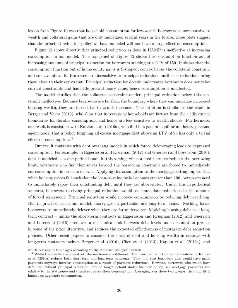
lesson from Figure 10 was that household consumption for low-wealth borrowers is unresponsive towealth and collateral gains that are only monetized several years in the future, these plots suggestthat the principal reduction policy we have modeled will not have a large effect on consumption.

Figure 12 shows directly that principal reduction as done in HAMP is ineffective at increasingconsumption in our model. The top panel of Figure 12 shows the consumption function out ofincreasing amounts of principal reduction for borrowers starting at a LTV of 150. It shows that theconsumption function out of home equity gains is S-shaped, convex below the collateral constraintand concave above it. Borrowers are insensitive to principal reductions until such reductions bringthem close to their constraint. Principal reduction for deeply underwater borrowers does not relaxcurrent constraints and has little precautionary value, hence consumption is unaffected.

The model clarifies that the collateral constraint renders principal reduction below this con-straint ineffective. Because borrowers are far from the boundary where they can monetize increasedhousing wealth, they are insensitive to wealth increases. The intuition is similar to the result inBerger and Vavra (2015), who show that in recessions households are farther from their adjustmentboundaries for durable consumption, and hence are less sensitive to wealth shocks. Furthermore,our result is consistent with Kaplan et al. (2016a), who find in a general equilibrium heterogeneous-agent model that a policy forgiving all excess mortgage debt above an LTV of 95 has only a trivialeffect on consumption.49

Our result contrasts with debt overhang models in which forced deleveraging leads to depressedconsumption. For example, in Eggertsson and Krugman (2012) and Guerrieri and Lorenzoni (2016),debt is modeled as a one-period bond. In this setting, when a credit crunch reduces the borrowinglimit, borrowers who find themselves beyond the borrowing constraint are forced to immediatelycut consumption in order to delever. Applying this assumption to the mortgage setting implies thatwhen housing prices fall such that the loan-to-value ratio becomes greater than 100, borrowers needto immediately repay their outstanding debt until they are abovewater. Under this hypotheticalscenario, borrowers receiving principal reduction would see immediate reductions in the amountof forced repayment. Principal reduction would increase consumption by reducing debt overhang.But in practice, as in our model, mortgages in particular are long-term loans. Nothing forcesborrowers to immediately delever when they are far underwater. Modeling housing debt as a long-term contract – unlike the short-term contracts in Eggertsson and Krugman (2012) and Guerrieriand Lorenzoni (2016)– removes a mechanical link between debt levels and consumption presentin some of the prior literature, and reduces the expected effectiveness of mortgage debt reductionpolicies. Other recent papers to consider the effect of debt and housing wealth in settings withlong-term contracts include Berger et al. (2016), Chen et al. (2013), Kaplan et al. (2016a), and

which is rising at these ages according to the standard life-cycle pattern.49While the results are consistent, the mechanism is different. The principal reduction policy modeled in Kaplan

et al. (2016a) reduces both short-term and long-term payments. They find that borrowers who would have madepayments anyways increase consumption as a result of payment reductions. However, borrowers who would havedefaulted without principal reduction, but no longer default under the new policy, see mortgage payments riserelative to the status-quo and therefore reduce their consumption. Averaging over these two groups, they find littleimpact on aggregate consumption.

36

Justiniano et al. (2015).

6.4.4 Consumption Response to Principal Reduction Under Alternative Parameter-izations

In our model, principal reduction is ineffective under a variety of alternative parameterizations.Table 8 reports the MPC for the principal reduction policy experiment described above undervarious alternative assumptions. The baseline MPC is 0.3 cents per dollar of mortgage principalreduced. This is similar to the 0.2 cent estimate in our empirical results. Changing borrower age,discount rate, and risk aversion has little impact on the MPC.

Principal reduction remains ineffective even when borrowers have modest access to liquidity.To show this, we calculated the effect of principal reduction assuming households had access to anunused HELOC line worth $20,000, which is twice the amount available to the average householdwith a HELOC in the 2015 New York Fed Consumer Credit Panel Federal Reserve (2015). TheMPC for this household is still only 0.9 cents. The reason is that households that have access toliquidity are optimizing incorporating this liquid buffer. Principal reduction does not increase theirbuffer in the near term, so has little effect on the value of maintaining this buffer. This explainswhy even borrowers who are actively saving or deleveraging, and therefore not literally at theirliquidity constraint, are unresponsive to principal reduction. Even when borrowers are saving forprecautionary reasons, the increase in housing wealth gained from principal reduction is of littleprecautionary value because it cannot be monetized for several years.

Generating a large consumption response requires an alternative unrealized economic environ-ment (relaxed collateral constraints and optimistic home price growth) or an alternative policy ofmore generous writedowns. Setting the collateral constraint to zero such that homeowners can leverup to 100 LTV generates a moderate MPC of 4.8 cents. Even though borrowers remain underwaterafter principal reduction, allowing them to monetize wealth starting at 100 LTV would have someimmediate precautionary value. Similarly, if households expected permanent real annual houseprice growth of 5% (equal to realized growth rates from 2000 to 2005), the MPC would be 6.2 centsbecause borrowers would expect to be able to monetize their housing wealth more quickly. Com-bining both of these assumptions about the economic environment generates a large MPC of 24.0cents. However, the period when principal reduction was implemented is exactly when neither ofthese conditions was likely to hold. In the aftermath of the crisis, home price growth expectationswere tepid and credit supply was tight.50

Although more generous principal reductions might have led to some observed consumptionresponse in the data, they would have been an inefficient way to raise consumption. For example,a writedown to 90 LTV with a relaxed collateral constraint raises consumption in our model.However, Figure 12 shows that all of the consumption increase is coming from the region near thecollateral constraint. This means that a policy of targeting deeply underwater borrowers with moregenerous writedowns will expend substantial resources in a region with no stimulative effect.

50See Department of Housing And Urban Development (2016) for house price expectations data and Corelogic(2016) for evidence of tightening collateral constraints.

37

6.4.5 Collateral Constraints Drive a Wedge Between MPC Out of Housing Wealthand MPC out of Cash

The inability to monetize housing wealth drives a wedge between an underwater borrower’s marginalpropensity to consume out of cash and their marginal propensity to consume out of housing wealth.This can be observed visually in the bottom panel of Figure 12. In this figure we take low-cash-on-hand borrowers at various LTV levels and plot the MPC out of $1 of cash or $1 of housing wealthgained by principal reduction.51 As in the empirical results in Mian et al. (2013), borrowers neartheir collateral constraint have a high MPC out of housing wealth gains. However, borrowers farunderwater are unresponsive to housing wealth changes even though they are highly responsiveto cash transfers. This highlights one way that housing wealth is special. Because it can onlybe monetized when borrowers have positive home equity above a collateral constraint, borrowersrespond less to housing wealth gains than they do to cash.

One implication of the wedge between cash and housing MPCs is that in a period where manyborrowers are underwater and collateral constraints have tightened, high leverage is a bad “tag”for targeting policies that increase housing wealth, even though it is a good “tag” for targetingpolicies trying to provide cash to borrowers with high MPCs. Our model suggests that low-wealth,underwater borrowers would have an MPC out of cash around 30 cents. The government spent anaverage of $0.30 to subsidize each dollar of principal forgiveness in HAMP, for a total governmentcost of $4.6 billion. Our model suggests that if the same amount of money had been spent on directtransfers to borrowers, the partial equilibrium spending increase would have been $1.4 billion, tentimes more than even the upper bound of our estimates for the consumption response to principalforgiveness would suggest. Policies seeking to raise aggregate demand by increasing the housingwealth of leveraged borrowers will be ineffective precisely when policymakers might otherwise wantto use them.

The low MPC out of housing wealth for underwater borrowers can help explain the sluggishresponse to house price gains during the recent recovery (Mian and Sufi 2014a). The borrowersordinarily most responsive to wealth gains may have found themselves unable to translate increasedhousing wealth into disposable wealth. This also points to a limitation of one of Fisher’s policyrecommendations for reversing “debt deflations” (Fisher 1933). He suggests reflating asset prices.Our results suggest that this may be ineffective at increasing demand for those who are underwaterunless pursued aggressively enough to bring them into positive equity.

51In this experiment, housing payments fall immediately when debt is reduced, unlike in Section 6.4.3 where wedelayed payment relief in order to mimic principal reduction in HAMP. We consider the average household from ourpolicy experiment, so we set cash-on-hand to 0.85.

38

7 Conclusion

This paper empirically and theoretically evaluates the impact of substantial mortgage principalreductions. Our empirical analysis exploits a distinctive government policy that allows us to isolatethe effects of reducing long-term payments and increasing home equity while controlling for short-term payments. Using regression discontinuity and difference-in-differences research designs, we findthat principal reductions have no short-term impact on default, durable consumption, or nondurableconsumption for borrowers who remain underwater. We build a quantitative life-cycle model witha housing asset and default to help interpret these empirical findings. The model clarifies thata borrower’s short-term constraints govern their response to long-term debt obligations. Whendefaulting imposes short-term utility costs, default is more responsive to cash-flow shocks than tofuture debt burdens. When principal reductions do not push borrowers sufficiently above waterso as to relax collateral constraints, consumption is unaffected because borrowers are unable tomonetize increased housing wealth.

Although we find that principal reductions have no impact in the short-term, an interestingavenue for future research will be to estimate the long-term impact. Eventually, borrowers whoreceived more substantial reductions will regain positive home equity. When faced with an incomeor expenditure shock, instead of defaulting and facing foreclosure, borrowers will be able to selltheir home. Similarly, borrowers who received principal reductions will more quickly gain enoughhome equity to overcome their collateral constraint, leading to increases in their borrowing capacity.In future work, we hope to study both of these effects.

A second natural experiment that will emerge over time comes from expected payment increases.Although payments for both modification groups are fixed for five years, they begin rising in yearsix as the temporary interest rate reduction is phased out. This will generate a completely expectednegative shock to disposable income. Prior work on mortgage payments has focused on paymentreductions which increase disposable income. In these cases, failure to increase consumption beforepayments fall can be attributed either to liquidity constraints or to bounded rationality. But insettings with predictable reductions in disposable income, even liquidity constrained householdsshould cut spending preemptively. In prior work we have found that unemployed agents fail to cutspending ahead of predictable exhaustion of their unemployment benefits (Ganong and Noel 2016).The expected mortgage payment increases that will eventually happen for HAMP borrowers willprovide a new way to test between the explanations for consumer sensitivity to expected changesin disposable income.

39

ReferencesAdelino, M., Schoar, A., and Severino, F. (2016). Loan Origination and Defaults in the MortgageCrisis: The Role of the Middle Class. Review of Financial Studies, 29(7):1635–1670.

Agarwal, S., Amromin, G., Ben-David, I., Chomsisengphat, S., Piskorski, T., and Seru, A. (2016a).Policy Intervention in Debt Renegotiation: Evidence from the Home Affordable ModificationProgram. Research Paper 3459, Stanford University, Graduate School of Business.

Agarwal, S., Amromin, G., Ben-David, I., Chomsisengphet, S., and Evanoff, D. D. (2011). The roleof securitization in mortgage renegotiation. Journal of Financial Economics, 102(3):559–578.

Agarwal, S., Amromin, G., Chomsisengphet, S., Piskorski, T., Seru, A., and Yao, V. W. (2015).Mortgage Refinancing, Consumer Spending, and Competition: Evidence from the Home Afford-able Refinancing Program. SSRN Scholarly Paper ID 2662906, Social Science Research Network,Rochester, NY.

Agarwal, S., Chomsisengphet, S., Mahoney, N., and Stroebel, J. (2016b). Do Banks Pass ThroughCredit Expansions? Asymmetric Information and the Marginal Profitability of Consumer Lend-ing During the Great Recession. SSRN Electronic Journal.

Aiyagari, S. R. (1994). Uninsured Idiosyncratic Risk and Aggregate Saving. The Quarterly Journalof Economics, 109(3):659–84.

Athey, S. and Imbens, G. (2016). The State of Applied Econometrics - Causality and PolicyEvaluation. arXiv:1607.00699 [stat].

Attanasio, O. P., Blow, L., Hamilton, R., and Leicester, A. (2009). Booms and Busts: Consumption,House Prices and Expectations. Economica, 76(301):20–50.

Berger, D., Guerrieri, V., Lorenzoni, G., and Vavra, J. (2016). House Prices and Consumer Spend-ing. Working Paper, University of Chicago and Northwester University.

Berger, D. and Vavra, J. (2015). Consumption Dynamics During Recessions. Econometrica,83(1):101–154.

Bernstein, A. (2015). Household Debt Overhang and Labor Supply. SSRN Scholarly Paper ID2700781, Social Science Research Network, Rochester, NY.

Bhutta, N., Dokko, J., and Shan, H. (2011). Consumer Ruthlessness and Mortgage Default Dur-ing the 2007-2009 Housing Bust. SSRN Scholarly Paper ID 1626969, Social Science ResearchNetwork, Rochester, NY.

Cagetti, M. (2003). Wealth Accumulation over the Life Cycle and Precautionary Savings. Journalof Business & Economic Statistics, 21(3):339–353.

Calonico, S., Cattaneo, M. D., and Titiunik, R. (2014). Robust Nonparametric Confidence Intervalsfor Regression-Discontinuity Designs. Econometrica, 82(6):2295–2326.

Campbell, J. Y. and Cocco, J. F. (2007). How do house prices affect consumption? Evidence frommicro data. Journal of Monetary Economics, 54(3):591–621.

Campbell, J. Y. and Cocco, J. F. (2015). A Model of Mortgage Default. Journal of Finance,70(4):1495–1554.

41

Carroll, C. (2012). Solution Methods for Microeconomic Dynamic Stochastic Optimization Prob-lems. Mimeo, Johns Hopkins Universtiy.

Carroll, C. D. (1992). The Buffer-Stock Theory of Saving: Some Macroeconomic Evidence. Brook-ings Papers on Economic Activity, 1992(2):61–156.

Carroll, C. D. (1997). Buffer-Stock Saving and the Life Cycle/Permanent Income Hypothesis. TheQuarterly Journal of Economics, 112(1):1–55.

Carroll, C. D. (2006). The method of endogenous gridpoints for solving dynamic stochastic opti-mization problems. Economics Letters, 91(3):312–320.

Carroll, C. D., Otsuka, M., and Slacalek, J. (2011). How Large Are Housing and Financial WealthEffects? A New Approach. Journal of Money, Credit and Banking, 43(1):55–79.

Carter, G. (2012). Housing Units With Negative Equity, 1997 to 2009. Cityscape, 14(1):149–165.

Case, K. E., Quigley, J. M., and Shiller, R. J. (2013). Wealth Effects Revisited: 1975-2012. WorkingPaper 18667, National Bureau of Economic Research.

Chen, H., Michaux, M., and Roussanov, N. L. (2013). Houses as ATMs? Mortgage Refinancingand Macroeconomic Uncertainty. SSRN Scholarly Paper ID 2024392, Social Science ResearchNetwork, Rochester, NY.

Clara, N. and Cocco, J. F. (2016). An Analysis of Consumer Debt Restructuring Policies. TechnicalReport 480, Society for Economic Dynamics.

Corelogic (2016). Home Equity Lending Landscape. White Paper.

Cowley, S. (2017). Foreclosure Prevention Returns to the Unknown. The NewYork Times, https://www.nytimes.com/2017/01/25/business/dealbook/foreclosure-prevention-mortgage-lending.html, January 25, 2017.

DeFusco, A. A. (2016). Homeowner Borrowing and Housing Collateral: New Evidence from Ex-piring Price Controls. SSRN Scholarly Paper ID 2696677, Social Science Research Network,Rochester, NY.

Department of Housing And Urban Development, U. (2016). Hous-ing Scorecard. HUD Report, September 2016, Availabel at:http://portal.hud.gov/hudportal/HUD?src=/initiatives/Housing_Scorecard.

Diaz, A. and Luengo-Prado, M. J. (2008). On the user cost and homeownership. Review of EconomicDynamics, 11(3):584–613.

DiMaggio, M., Kermani, A., Keys, B., Piskorski, T., Ramchaan, R., Seru, A., and Yao, V. (2017).Interest Rate Pass-Through: Mortgage Rates, Household Consumption, and Voluntary Delever-aging. American Economic Review, 107(11):3550–3588.

Disney, R., Gathergood, J., and Henley, A. (2010). House Price Shocks, Negative Equity, AndHousehold Consumption In The United Kingdom 4. Journal of the European Economic Associ-ation, 8(6):1179–1207.

42

Dobbie, W. and Song, J. (2016). Debt Relief or Debt Restructuring? Evidence From an Experimentwith Distressed Credit Card Borrowers. Working Paper, Princeton University and Social SecurityAdministration.

Eberly, J. and Krishnamurthy, A. (2014). Efficient Credit Policies in a Housing Debt Crisis. Brook-ings Papers on Economic Activity, 49(2 (Fall)):73–136.

Eggertsson, G. B. and Krugman, P. (2012). Debt, deleveraging, and the liquidity trap: a Fisher-Minsky-Koo approach. The quarterly journal of economics, 127(3):1469–1518.

Ehrlich, G. and Perry, J. (2015). Do Large-Scale Refinancing Programs Reduce Mortgage Defaults?Evidence From a Regression Discontinuity Design: Working Paper 2015-06. Working Paper50871, Congressional Budget Office.

Experian and Wyman, O. (2009). Understanding Strategic Default in Mortgages Part 1. WhitePaper.

Federal Reserve, N. Y. (2015). Quarterly Report on Household Debt and Credit. Federal ReserveBank of New York, Research and Statistics Group, November 2015.

Federal Reserve, U. S. (2014). The 2013 Federal Reserve Payments Study. The Federal ReserveSystem.

Feldstein, M. (2009). How to Save an ’Underwater’ mortgage. Wall Street Journal, August 7, 2009.

Fisher, I. (1933). The Debt-Deflation Theory of Great Depressions. Econometrica, pages 337–357.

Foote, C. L., Gerardi, K., and Willen, P. S. (2008). Negative equity and foreclosure: Theory andevidence. Journal of Urban Economics, 64(2):234–245.

Fuster, A. and Willen, P. (2015). Payment Size, Negative Equity, and Mortgage Default. FederalReserve Bank of New York Staff Reports, No. 582.

Fuster, A. and Willen, P. (2017). Payment Size, Negative Equity, and Mortgage Default. AmericanEconomic Journal: Economic Policy, 9(4):167–191.

Gabriel, S. A., Iacoviello, M. M., and Lutz, C. (2016). A Crisis of Missed Opportunities? ForeclosureCosts and Mortgage Modification During the Great Recession. SSRN Scholarly Paper ID 2831830,Social Science Research Network, Rochester, NY.

Ganong, P. and Noel, P. (2017). Consumer Spending During Unemployment: Positive and Norma-tive Implications.

Geanakoplos, J. and Koniak, S. (2009). Matters of Principal. The New York Times, March 4, 2009.

Geithner, T. (2014). Stress Test. Broadway Books.

Gerardi, K., Herkenhoff, K. F., Ohanian, L. E., and Willen, P. S. (2015). Can’t Pay or Won’t Pay?Unemployment, Negative Equity, and Strategic Default. NBER Working Paper 21630, NationalBureau of Economic Research, Inc.

Ghent, A. C. and Kudlyak, M. (2011). Recourse and Residential Mortgage Default: Evidence fromUS States. The Review of Financial Studies, 24(9):3139–3186.

43

Goldfarb, Z. (2012). Economists, Obama Administration at Odds Over Role of Mortgage Debt inRecovery. The Washington Post, November 22, 2012.

Guerrieri, V. and Lorenzoni, G. (2016). Credit Crises, Precautionary Savings, and the LiquidityTrap. Working Paper, University of Chicago and Northwestern University.

Guiso, L., Sapienza, P., and Zingales, L. (2013). The Determinants of Attitudes toward StrategicDefault on Mortgages. Journal of Finance, 68(4):1473–1515.

Guren, A. and McQuade, T. (2015). How do Forecolosures Exacerbate Housing Downturns? Work-ing Paper, Boston University and Stanford University.

Guren, A. M., Krishnamurthy, A., and McQuade, T. J. (2017). Mortgage Design in an EquilibriumModel of the Housing Market. working paper.

Guvenen, F., Ozkan, S., and Song, J. (2014). The Nature of Countercyclical Income Risk. Journalof Political Economy, 122(3):621–660.

Haughwout, A., Okah, E., and Tracy, J. (2016). Second Chances: Subprime Mortgage Modificationand Redefault. Journal of Money, Credit and Banking, 48(4):771–793.

Hembre, E. (2014). HAMP, Home Attachment, and Mortgage Default. Working Paper, Universityof Wisconsin.

Herkenhoff, K. F. and Ohanian, L. E. (2015). The Impact of Foreclosure Delay on U.S. Employment.Working Paper 21532, National Bureau of Economic Research.

Himmelberg, C., Mayer, C., and Sinai, T. (2005). Assessing High House Prices: Bubbles, Funda-mentals and Misperceptions. Journal of Economic Perspectives, 19(4):67–92.

Holden, S., Kelly, A., McManus, D. A., Scharlemann, T. C., Singer, R., and Worth, J. (2012). TheHAMP NPV Model: Development and Early Performance. SSRN Scholarly Paper ID 2194279,Social Science Research Network, Rochester, NY.

Hsu, J. W., Matsa, D. A., and Melzer, B. (2014). Positive Externalities of Social Insurance:Unemployment Insurance and Consumer Credit. SSRN Scholarly Paper ID 2185198, SocialScience Research Network, Rochester, NY.

Imbens, G. and Kalyanaraman, K. (2012). Optimal Bandwidth Choice for the Regression Discon-tinuity Estimator. Review of Economic Studies, 79(3):933–959.

Justiniano, A., Primiceri, G. E., and Tambalotti, A. (2015). Household leveraging and deleveraging.Review of Economic Dynamics, 18(1):3–20.

Kaplan, G., Mitman, K., and Violante, G. L. (2016a). Consumption and House Prices in the GreatRecession. Working Paper.

Kaplan, G., Mitman, K., and Violante, G. L. (2016b). Non-Durable Consumption and Housing NetWorth in the Great Recession: Evidence from Easily Accessible Data. SSRN Scholarly Paper ID2777320, Social Science Research Network, Rochester, NY.

Kau, J. B., Keenan, D. C., and Taewon Kim (1993). Transaction costs, suboptimal terminationand default probabilities. Journal of the American Real Estate & Urban Economics Association,21(3):247.

44

Keys, B. J., Piskorski, T., Seru, A., and Yao, V. W. (2014). Mortgage Rates, Household BalanceSheets, and the Real Economy. SSRN Scholarly Paper ID 2505691, Social Science ResearchNetwork, Rochester, NY.

Kruger, S. A. (2016). The Effect of Mortgage Securitization on Foreclosure and Modification. SSRNScholarly Paper ID 2794122, Social Science Research Network, Rochester, NY.

Lee, D. S. and Lemieux, T. (2010). Regression Discontinuity Designs in Economics. Journal ofEconomic Literature, 48(2):281–355.

McCrary, J. (2008). Manipulation of the running variable in the regression discontinuity design: Adensity test. Journal of Econometrics, 142(2):698–714.

Mckay, A., Nakamura, E., and Steinsson, J. (2016). The Power of Forward Guidance Revisited.American Economic Review, 106(10):3133–3158.

Mian, A., Rao, K., and Sufi, A. (2013). Household Balance Sheets, Consumption, and the EconomicSlump. The Quarterly Journal of Economics, 128(4):1687–1726.

Mian, A. and Sufi, A. (2010). Household Leverage and the Recession of 2007-09. IMF EconomicReview, 58(1):74–117.

Mian, A. and Sufi, A. (2014a). House Price Gains and U.S. Household Spending from 2002 to 2006.Working Paper 20152, National Bureau of Economic Research.

Mian, A. and Sufi, A. (2014b). Why Tim Geithner is wrong on homeowner debt relief. TheWashington Post, May 14, 2014.

Mitman, K. (2016). Macroeconomic Effects of Bankruptcy and Foreclosure Policies. AmericanEconomic Review, 106(8):2219–2255.

Narasiman, V. (2016). What do Adjustable-Rate Mortgage Resets Say About Household Con-sumption Behavior and the Income Channel of Monetary Policy? Working Paper, HarvardUniversity.

Palmer, C. (2015). Why Did So Many Subprime Borrowers Default During the Crisis: Loose Creditor Plummeting Prices? Working Paper, University of California at Berkeley.

Poterba, J. and Sinai, T. (2008). Tax Expenditures for Owner-Occupied Housing: Deductions forProperty Taxes and Mortgage Interest and the Exclusion of Imputed Rental Income. AmericanEconomic Review, 98(2):84–89.

Romer, C. (2011). Policy Responses to the Great Recession: The Interaction of Leadership andEconomic Ideas. Speech, Ohio State University, December 1, 2011.

Scharlemann, T. and Shore, S. H. (2017). The Effect of Mortgage Payment Size on Default andPrepayment: Evidence from HAMP Resets. working paper.

Scharlemann, T. C. and Shore, S. H. (2016). Does Reducing Negative Equity Prevent MortgageDefault? Evidence from HAMP’s Principal Reduction Alternative. Review of Financial Studies,forthcoming.

Schelkle, T. (2016). Mortgage Default During the U.S. Mortgage Crisis. Working Paper, Universityof Cologne.

45

Schwartz, M. and Wilson, E. (2008). Who Can Afford To Live in a Home? A Look at Data fromthe 2006 American Community Survey. Technical report, US Census Bureau 2008.

Stanton, R. and Wallace, N. (1998). Mortgage Choice: What’s the Point? Real Estate Economics,26(2):173–205.

Tracy, J. and Wright, J. (2012). Payment Changes and Default Risk: The Impact of Refinancingon Expected Credit Losses. Federal Reserve Bank of New York Staff Reports.

Treasury Department, U. (2014a). Making Home Affordable Program Performance Report ThroughThe Second Quarter of 2014. Treasury Department Report.

Treasury Department, U. (2014b). MHA Data File User Guide. Treausry White Paper.

Treasury Department, U. S. (2014c). Making Home Affordable Program Handbook for Servicers ofNon-GSE Mortgages. Version 4.4.

Winkler, R. (2010). Report Shows Strategic Defaults Increasing. Reuters, March 26, 2010.

Zingales, L. (2010). The Menace of Strategic Default. City Journal, Spring 2010.

46

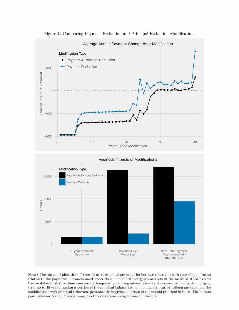
Figure 1: Comparing Payment Reduction and Principal Reduction Modifications

● ● ● ● ●

●● ● ● ● ● ● ● ● ● ● ● ● ● ● ●

●

●

●

●

●

●

●

● ● ● ● ●●

● ●● ●

●

●

−8000

−4000

0

4000

0 10 20 30 40Years Since Modification

Cha

nge

in A

nnua

l Pay

men

t

Modification Type

● Payment & Principal Reduction

Payment Reduction

Average Annual Payment Change After Modification

0

25000

50000

75000

1−year PaymentReduction

Balance DueReduction

NPV Total PaymentReduction at 4%

Interest Rate

Dol

lars

Modification Type

Payment & Principal Reduction

Payment Reduction

Financial Impacts of Modifications

Notes: The top panel plots the difference in average annual payments for borrowers receiving each type of modificationrelative to the payments borrowers owed under their unmodified mortgage contracts in the matched HAMP creditbureau dataset. Modifications consisted of temporarily reducing interest rates for five years, extending the mortgageterm up to 40 years, turning a portion of the principal balance into a non-interest-bearing balloon payment, and formodifications with principal reduction, permanently forgiving a portion of the unpaid principal balance. The bottompanel summarizes the financial impacts of modifications along various dimensions.

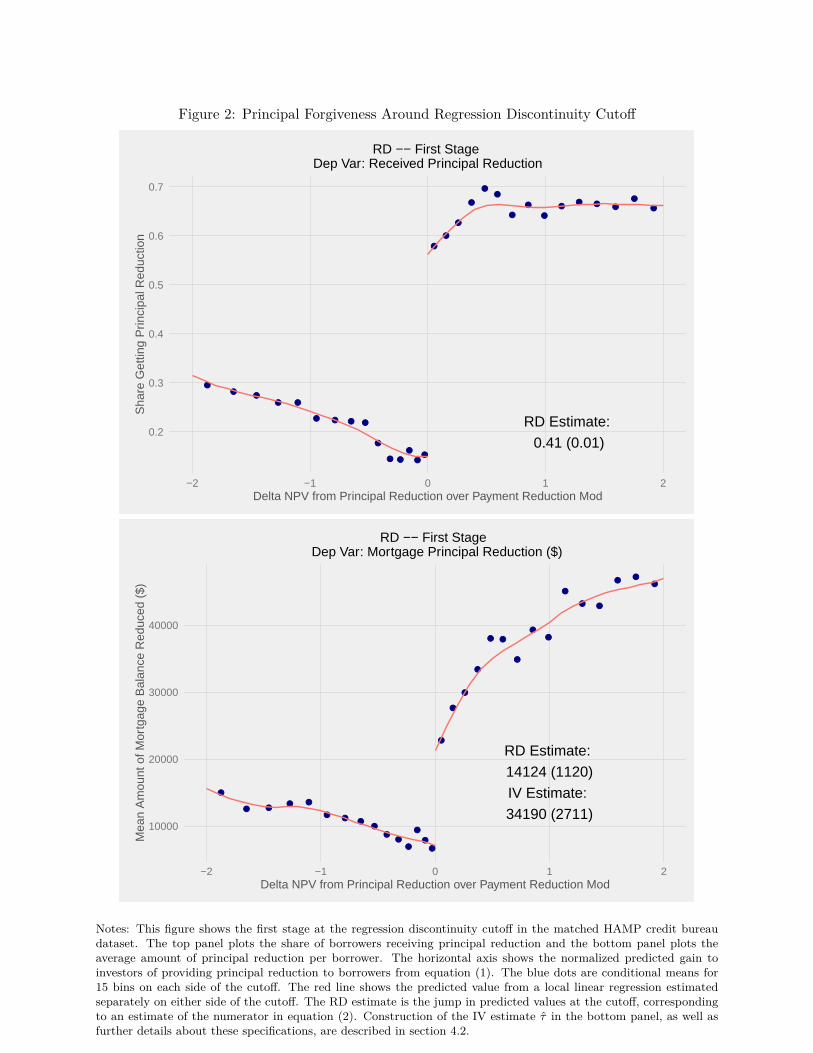
Figure 2: Principal Forgiveness Around Regression Discontinuity Cutoff

●●

●● ●

● ● ● ●

●

● ●

●

●●

●

●

●

●

●●

●

●

●

●● ● ●

●

●

RD Estimate: 0.41 (0.01)

0.2

0.3

0.4

0.5

0.6

0.7

−2 −1 0 1 2Delta NPV from Principal Reduction over Payment Reduction Mod

Sha

re G

ettin

g P

rinci

pal R

educ

tion

RD −− First Stage Dep Var: Received Principal Reduction

●

● ●● ●

● ● ●●

●●

●

●

●●

●

●

●

●

● ●

●

●●

●

● ●

● ●●

RD Estimate:

14124 (1120)IV Estimate:

34190 (2711)10000

20000

30000

40000

−2 −1 0 1 2Delta NPV from Principal Reduction over Payment Reduction Mod

Mea

n A

mou

nt o

f Mor

tgag

e B

alan

ce R

educ

ed (

$)

RD −− First Stage Dep Var: Mortgage Principal Reduction ($)

Notes: This figure shows the first stage at the regression discontinuity cutoff in the matched HAMP credit bureaudataset. The top panel plots the share of borrowers receiving principal reduction and the bottom panel plots theaverage amount of principal reduction per borrower. The horizontal axis shows the normalized predicted gain toinvestors of providing principal reduction to borrowers from equation (1). The blue dots are conditional means for15 bins on each side of the cutoff. The red line shows the predicted value from a local linear regression estimatedseparately on either side of the cutoff. The RD estimate is the jump in predicted values at the cutoff, correspondingto an estimate of the numerator in equation (2). Construction of the IV estimate τ̂ in the bottom panel, as well asfurther details about these specifications, are described in section 4.2.

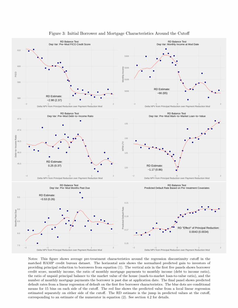
Figure 3: Initial Borrower and Mortgage Characteristics Around the Cutoff

●●

●●

●●

● ●

● ●

●

●●

●●

●

●

●

●

●

●

●

●

●

●

●

●

●

●

●

RD Estimate: −2.98 (2.37)

580

590

600

610

−2 −1 0 1 2Delta NPV from Principal Reduction over Payment Reduction Mod

FIC

O

RD Balance Test Dep Var: Pre−Mod FICO Credit Score

●

●

●

●

●

●

●

●

●

●

●

●

●

●

●

●

●

●

●

●

● ●

●●

●

●

●

●●

●RD Estimate:

−66 (65)5000

5100

5200

5300

−2 −1 0 1 2Delta NPV from Principal Reduction over Payment Reduction Mod

Mon

thly

Inco

me

RD Balance Test Dep Var: Monthly Income at Mod Date

●

●●

●

●

●

●

●

●

●

●

●

●

●

●

●

● ●

●

●

●

●

●

●

●

●

●

●

●

●

RD Estimate: 0.25 (0.37)

45.5

46.0

46.5

47.0

47.5

−2 −1 0 1 2Delta NPV from Principal Reduction over Payment Reduction Mod

Deb

t−to

−In

com

e R

atio

RD Balance Test Dep Var: Pre−Mod Debt−to−Income Ratio

●

●

●

●● ●

●●

●

●

●

●

●

●

●

●

●

●

●

●

●

●

●●

● ●

● ●

●

●

RD Estimate: −1.17 (0.86)

120

125

130

135

−2 −1 0 1 2Delta NPV from Principal Reduction over Payment Reduction Mod

MT

M L

TV

RD Balance Test Dep Var: Pre−Mod Mark−to−Market Loan−to−Value

● ●

●

●

●

●

●

●

●

●

●

●

●

●

●

●●

●

●

●

●

●

●

●

●

●

●●

●

●

RD Estimate: −0.53 (0.26)

7.5

8.0

8.5

9.0

9.5

−2 −1 0 1 2Delta NPV from Principal Reduction over Payment Reduction Mod

Mon

ths

Pas

t Due

RD Balance Test Dep Var: Pre−Mod Months Past Due

●

●

●

●

●

●

●

●

●●

●

● ●

●●

●

●●

●

●

● ●●

●

●

●

●

●

●

●

RD "Effect" of Principal Reduction: 0.0043 (0.0034)

0.15

0.17

0.19

0.21

−2 −1 0 1 2Delta NPV from Principal Reduction over Payment Reduction Mod

Pre

dict

ed D

efau

lt R

ate

RD Balance Test Predicted Default Rate Based on Pre−treatment Covariates

Notes: This figure shows average pre-treatment characteristics around the regression discontinuity cutoff in thematched HAMP credit bureau dataset. The horizontal axis shows the normalized predicted gain to investors ofproviding principal reduction to borrowers from equation (1). The vertical axis in the first five panels shows borrowercredit score, monthly income, the ratio of monthly mortgage payments to monthly income (debt to income ratio),the ratio of unpaid principal balance to the market value of the house (mark-to-market loan-to-value ratio), and thenumber of monthly mortgage payments the borrower is past due at application date. The final panel shows predicteddefault rates from a linear regression of default on the first five borrower characteristics. The blue dots are conditionalmeans for 15 bins on each side of the cutoff. The red line shows the predicted value from a local linear regressionestimated separately on either side of the cutoff. The RD estimate is the jump in predicted values at the cutoff,corresponding to an estimate of the numerator in equation (2). See section 4.2 for details.

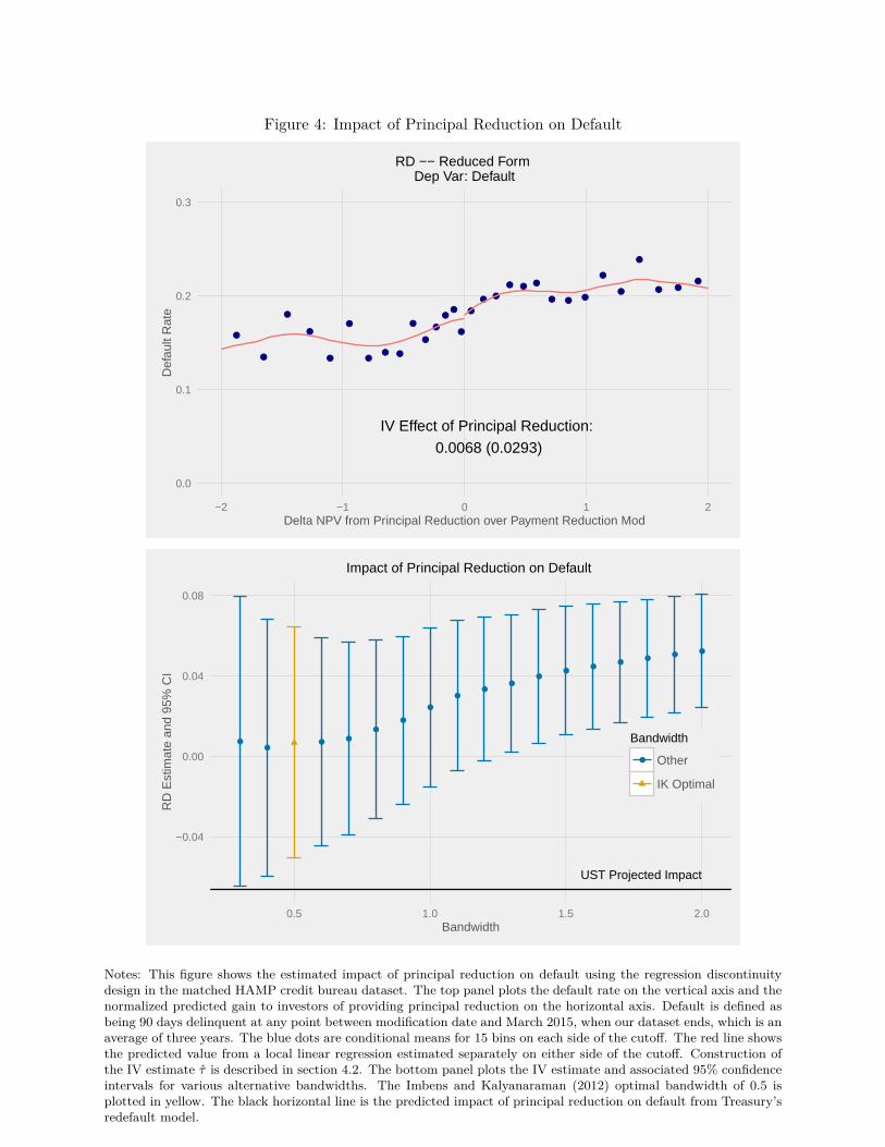
Figure 4: Impact of Principal Reduction on Default

●

●

●

●

●

●

●● ●

●

●

●

●●

●

●

● ●

● ● ●

● ● ●

●

●

●

● ●●

IV Effect of Principal Reduction:

0.0068 (0.0293)

0.0

0.1

0.2

0.3

−2 −1 0 1 2Delta NPV from Principal Reduction over Payment Reduction Mod

Def

ault

Rat

eRD −− Reduced Form

Dep Var: Default

●●

● ●

●

●

●

●●

●●

●●

●●

● ●

UST Projected Impact

−0.04

0.00

0.04

0.08

0.5 1.0 1.5 2.0Bandwidth

RD

Est

imat

e an

d 95

% C

I

Bandwidth

● Other

IK Optimal

Impact of Principal Reduction on Default

Notes: This figure shows the estimated impact of principal reduction on default using the regression discontinuitydesign in the matched HAMP credit bureau dataset. The top panel plots the default rate on the vertical axis and thenormalized predicted gain to investors of providing principal reduction on the horizontal axis. Default is defined asbeing 90 days delinquent at any point between modification date and March 2015, when our dataset ends, which is anaverage of three years. The blue dots are conditional means for 15 bins on each side of the cutoff. The red line showsthe predicted value from a local linear regression estimated separately on either side of the cutoff. Construction ofthe IV estimate τ̂ is described in section 4.2. The bottom panel plots the IV estimate and associated 95% confidenceintervals for various alternative bandwidths. The Imbens and Kalyanaraman (2012) optimal bandwidth of 0.5 isplotted in yellow. The black horizontal line is the predicted impact of principal reduction on default from Treasury’sredefault model.

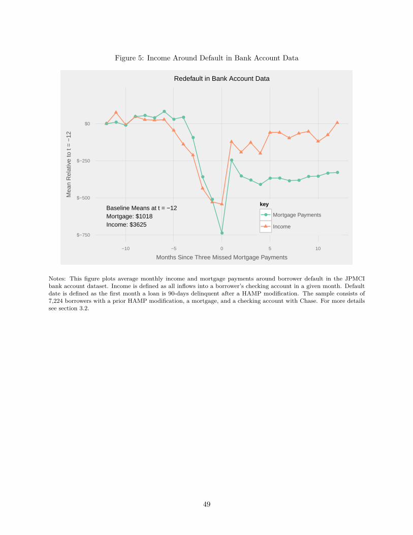
Figure 5: Income Around Default in Bank Account Data

● ●●

● ●●

●

●●

●

●

●

●

●

●●

●

● ●● ●

● ●● ●

Baseline Means at t = −12 Mortgage: $1018Income: $3625

$−750

$−500

$−250

$0

−10 −5 0 5 10

Months Since Three Missed Mortgage Payments

Mea

n R

elat

ive

to t

= −

12

key

● Mortgage Payments

Income

Redefault in Bank Account Data

Notes: This figure plots average monthly income and mortgage payments around borrower default in the JPMCIbank account dataset. Income is defined as all inflows into a borrower’s checking account in a given month. Defaultdate is defined as the first month a loan is 90-days delinquent after a HAMP modification. The sample consists of7,224 borrowers with a prior HAMP modification, a mortgage, and a checking account with Chase. For more detailssee section 3.2.

49

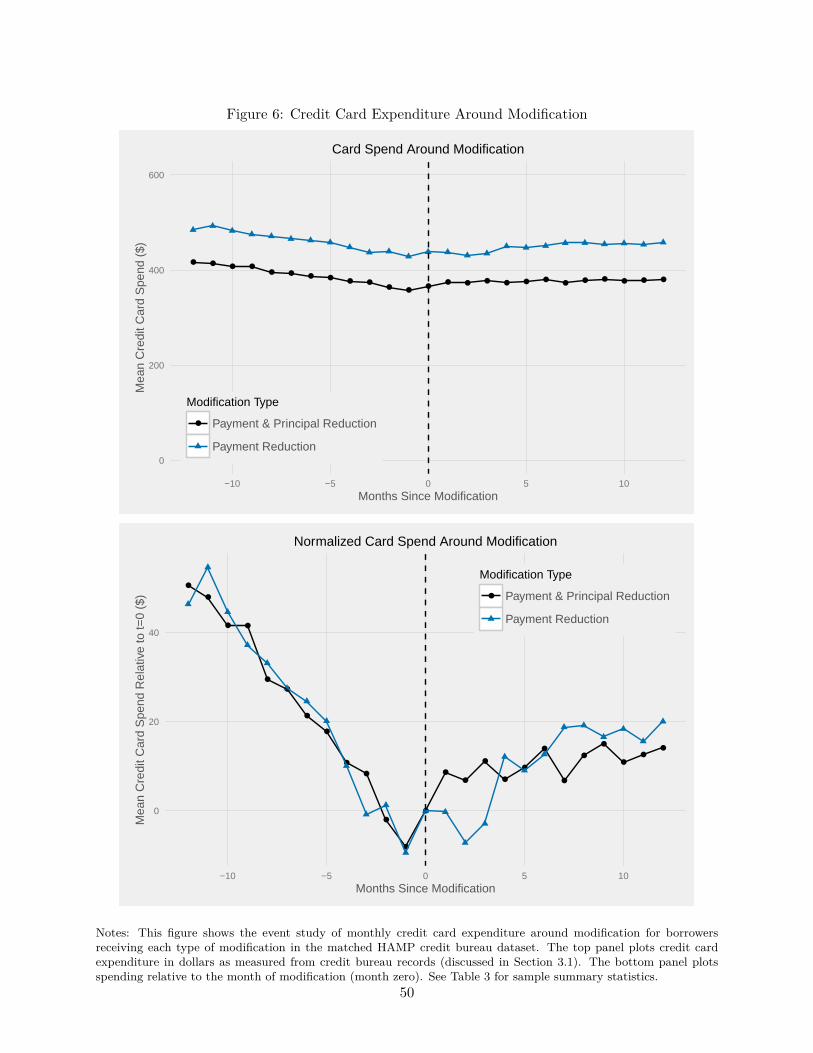
Figure 6: Credit Card Expenditure Around Modification

● ● ● ●● ● ● ● ● ●

● ●●

● ● ● ● ● ● ● ● ● ● ● ●

0

200

400

600

−10 −5 0 5 10Months Since Modification

Mea

n C

redi

t Car

d S

pend

($)

Modification Type

● Payment & Principal Reduction

Payment Reduction

Card Spend Around Modification

●

●

● ●

●

●

●

●

●

●

●

●

●

●●

●

●

●

●

●

●

●

●●

●

0

20

40

−10 −5 0 5 10Months Since Modification

Mea

n C

redi

t Car

d S

pend

Rel

ativ

e to

t=0

($)

Modification Type

● Payment & Principal Reduction

Payment Reduction

Normalized Card Spend Around Modification

Notes: This figure shows the event study of monthly credit card expenditure around modification for borrowersreceiving each type of modification in the matched HAMP credit bureau dataset. The top panel plots credit cardexpenditure in dollars as measured from credit bureau records (discussed in Section 3.1). The bottom panel plotsspending relative to the month of modification (month zero). See Table 3 for sample summary statistics.

50

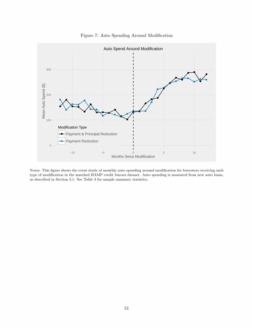
Figure 7: Auto Spending Around Modification

●

●

● ●

●

●

● ● ●

●

●

●

● ●

●

●●

●

●

●●

● ●

●

●

0

100

200

300

−10 −5 0 5 10Months Since Modification

Mea

n A

uto

Spe

nd (

$)

Modification Type

● Payment & Principal Reduction

Payment Reduction

Auto Spend Around Modification

Notes: This figure shows the event study of monthly auto spending around modification for borrowers receiving eachtype of modification in the matched HAMP credit bureau dataset. Auto spending is measured from new auto loans,as described in Section 3.1. See Table 3 for sample summary statistics.

51

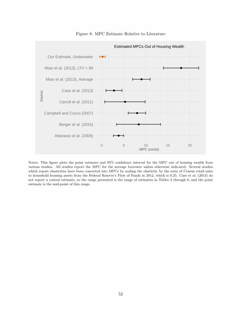
Figure 8: MPC Estimate Relative to Literature

●

●

●

●

●

●

●

●

Attanasio et al. (2009)

Berger et al. (2015)

Campbell and Cocco (2007)

Carroll et al. (2011)

Case et al. (2013)

Mian et al. (2013), Average

Mian et al. (2013), LTV > 90

Our Estimate, Underwater

0 5 10 15 20MPC (cents)

Sou

rce

Estimated MPCs Out of Housing Wealth

Notes: This figure plots the point estimate and 95% confidence interval for the MPC out of housing wealth fromvarious studies. All studies report the MPC for the average borrower unless otherwise indicated. Several studieswhich report elasticities have been converted into MPCs by scaling the elasticity by the ratio of Census retail salesto household housing assets from the Federal Reserve’s Flow of Funds in 2012, which is 0.25. Case et al. (2013) donot report a central estimate, so the range presented is the range of estimates in Tables 3 through 6, and the pointestimate is the mid-point of this range.

52

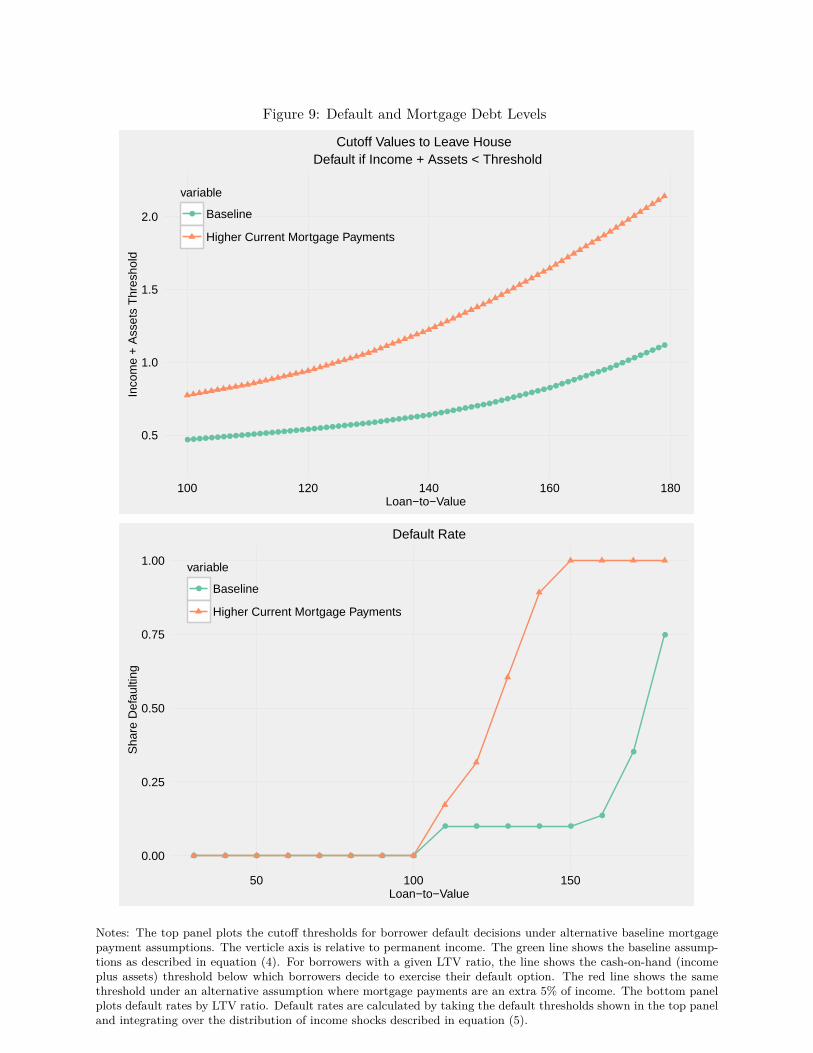
Figure 9: Default and Mortgage Debt Levels

●●●●●●●●●●●●●●●●●●●●●●●●●●●●●●●●●●●●●●●●●●●●●●●●●●●●●●●●●●●●●●●●●●●●●●●●●●●●●●●●

0.5

1.0

1.5

2.0

100 120 140 160 180Loan−to−Value

Inco

me

+ A

sset

s T

hres

hold

variable

● Baseline

Higher Current Mortgage Payments

Cutoff Values to Leave House Default if Income + Assets < Threshold

● ● ● ● ● ● ● ●

● ● ● ● ●

●

●

●

0.00

0.25

0.50

0.75

1.00

50 100 150Loan−to−Value

Sha

re D

efau

lting

variable

● Baseline

Higher Current Mortgage Payments

Default Rate

Notes: The top panel plots the cutoff thresholds for borrower default decisions under alternative baseline mortgagepayment assumptions. The verticle axis is relative to permanent income. The green line shows the baseline assump-tions as described in equation (4). For borrowers with a given LTV ratio, the line shows the cash-on-hand (incomeplus assets) threshold below which borrowers decide to exercise their default option. The red line shows the samethreshold under an alternative assumption where mortgage payments are an extra 5% of income. The bottom panelplots default rates by LTV ratio. Default rates are calculated by taking the default thresholds shown in the top paneland integrating over the distribution of income shocks described in equation (5).

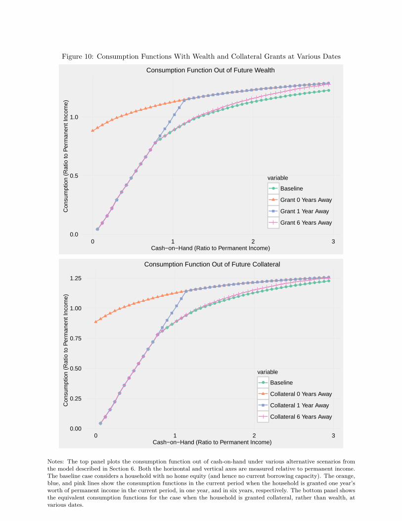
Figure 10: Consumption Functions With Wealth and Collateral Grants at Various Dates

●

●

●

●

●

●

●

●

●

●

●

●

●●

●●

●●

●●

●●

● ● ● ● ● ● ● ● ● ● ● ● ● ● ● ● ● ● ● ● ● ● ● ● ● ● ●

0.0

0.5

1.0

0 1 2 3Cash−on−Hand (Ratio to Permanent Income)

Con

sum

ptio

n (R

atio

to P

erm

anen

t Inc

ome)

variable

● Baseline

Grant 0 Years Away

Grant 1 Year Away

Grant 6 Years Away

Consumption Function Out of Future Wealth

●

●

●

●

●

●

●

●

●

●

●

●

●●

●●

●●

●●

●●

● ● ● ● ● ● ● ● ● ● ● ● ● ● ● ● ● ● ● ● ● ● ● ● ● ● ●

0.00

0.25

0.50

0.75

1.00

1.25

0 1 2 3Cash−on−Hand (Ratio to Permanent Income)

Con

sum

ptio

n (R

atio

to P

erm

anen

t Inc

ome)

variable

● Baseline

Collateral 0 Years Away

Collateral 1 Year Away

Collateral 6 Years Away

Consumption Function Out of Future Collateral

Notes: The top panel plots the consumption function out of cash-on-hand under various alternative scenarios fromthe model described in Section 6. Both the horizontal and vertical axes are measured relative to permanent income.The baseline case considers a household with no home equity (and hence no current borrowing capacity). The orange,blue, and pink lines show the consumption functions in the current period when the household is granted one year’sworth of permanent income in the current period, in one year, and in six years, respectively. The bottom panel showsthe equivalent consumption functions for the case when the household is granted collateral, rather than wealth, atvarious dates.

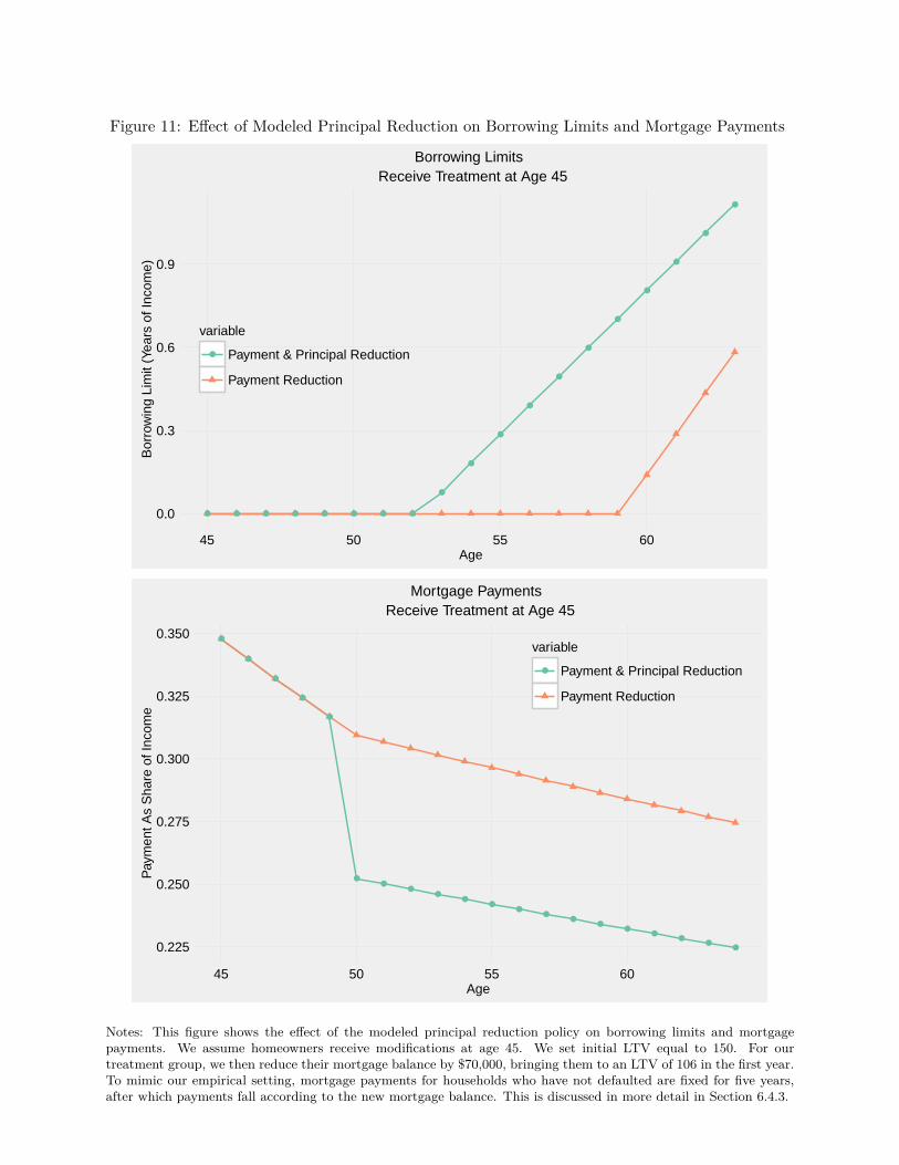
Figure 11: Effect of Modeled Principal Reduction on Borrowing Limits and Mortgage Payments

● ● ● ● ● ● ● ●

●

●

●

●

●

●

●

●

●

●

●

0.0

0.3

0.6

0.9

45 50 55 60Age

Bor

row

ing

Lim

it (Y

ears

of I

ncom

e)

variable

● Payment & Principal Reduction

Payment Reduction

Borrowing Limits Receive Treatment at Age 45

●

●

●

●

●

●●

●●

●●

●●

●●

●●

●●

●0.225

0.250

0.275

0.300

0.325

0.350

45 50 55 60Age

Pay

men

t As

Sha

re o

f Inc

ome

variable

● Payment & Principal Reduction

Payment Reduction

Mortgage Payments Receive Treatment at Age 45

Notes: This figure shows the effect of the modeled principal reduction policy on borrowing limits and mortgagepayments. We assume homeowners receive modifications at age 45. We set initial LTV equal to 150. For ourtreatment group, we then reduce their mortgage balance by $70,000, bringing them to an LTV of 106 in the first year.To mimic our empirical setting, mortgage payments for households who have not defaulted are fixed for five years,after which payments fall according to the new mortgage balance. This is discussed in more detail in Section 6.4.3.

Figure 12: Consumption and Mortgage Debt Levels

●●

●●

●●

●●

●●

●●

●●

●

●

●

●

●

●

●

●

●

●

●

●

●

●

●●

●●●●●●●●●●●●●●●●●●●●

0.6

0.7

0.8

0.9

1.0

050100150Loan−to−Value (> 100 is Underwater)

Con

sum

ptio

n (R

atio

to P

erm

anen

t Inc

ome)

variable

● Baseline

Consumption Function Out of Principal Forgiveness

●●

●

●

●

●

●

●

●

●

●●●●●●●

0.1

0.2

0.3

4080120160Loan−to−Value (> 100 is Underwater)

MP

C

variable

● Cash MPC

Housing Debt MPC

Marginal Propensity to Consume by Home Equity

Notes: The top panel plots the consumption function out of principal reduction. We begin borrowers at 150 LTVand give increasing amounts of principal reduction as necessary to hit a given LTV ratio. To mimic our empiricalsetting, mortgage payments for households who have not defaulted are fixed for five years, after which paymentsfall according to the new mortgage balance. The red arrow shows the treatment for the average borrower in thegovernment program. The dashed green line indicates the collateral constraint. The bottom panel plots the marginalpropensity to consume out of an additional dollar of cash or an additional dollar of housing wealth generated bymortgage debt forgiveness. In this panel mortgage debt forgiveness is assumed to translate immediately into reducedmortgage payments. Both panels are plotted for homeowners age 45 with initial assets of at at = 0.01 units ofpermanent income and income of yt = 0.85 units of permanent income.

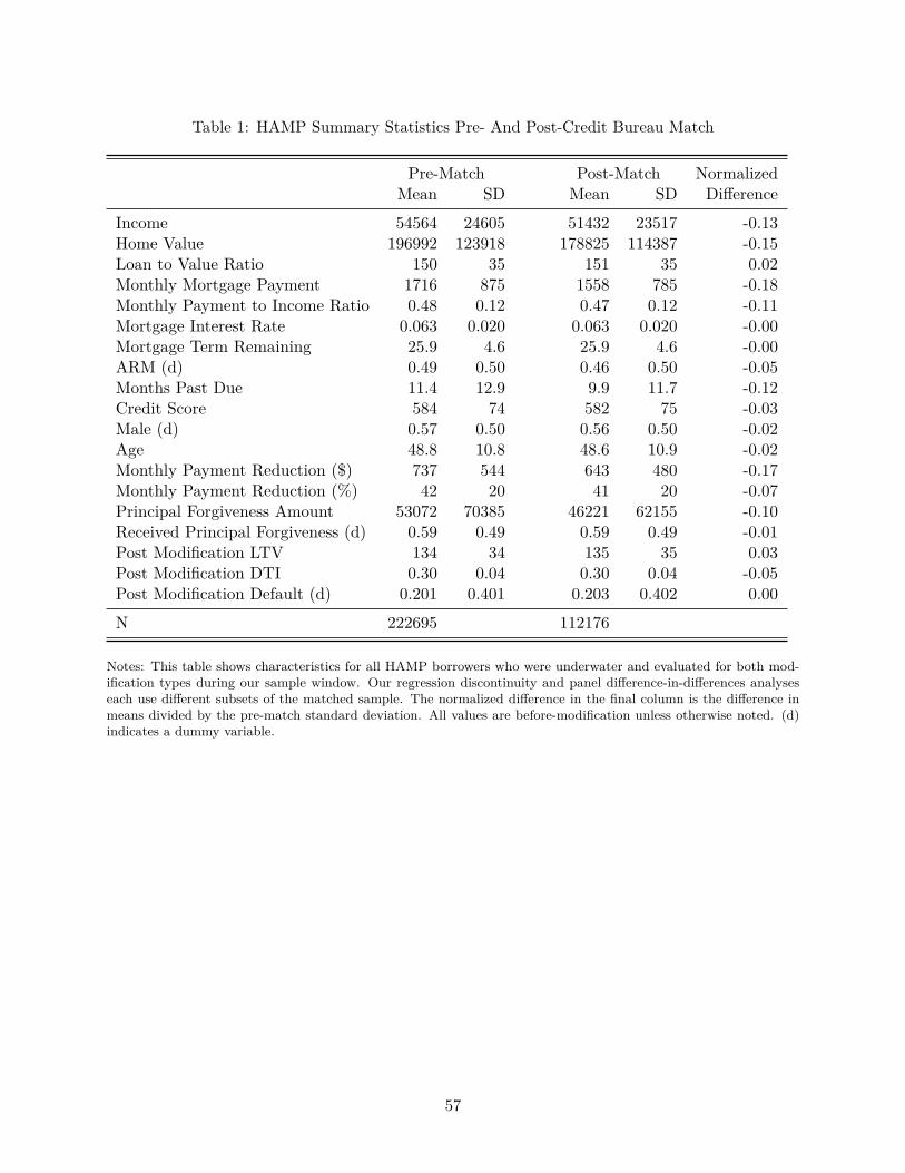
Table 1: HAMP Summary Statistics Pre- And Post-Credit Bureau Match

Pre-Match Post-Match NormalizedMean SD Mean SD Difference

Income 54564 24605 51432 23517 -0.13Home Value 196992 123918 178825 114387 -0.15Loan to Value Ratio 150 35 151 35 0.02Monthly Mortgage Payment 1716 875 1558 785 -0.18Monthly Payment to Income Ratio 0.48 0.12 0.47 0.12 -0.11Mortgage Interest Rate 0.063 0.020 0.063 0.020 -0.00Mortgage Term Remaining 25.9 4.6 25.9 4.6 -0.00ARM (d) 0.49 0.50 0.46 0.50 -0.05Months Past Due 11.4 12.9 9.9 11.7 -0.12Credit Score 584 74 582 75 -0.03Male (d) 0.57 0.50 0.56 0.50 -0.02Age 48.8 10.8 48.6 10.9 -0.02Monthly Payment Reduction ($) 737 544 643 480 -0.17Monthly Payment Reduction (%) 42 20 41 20 -0.07Principal Forgiveness Amount 53072 70385 46221 62155 -0.10Received Principal Forgiveness (d) 0.59 0.49 0.59 0.49 -0.01Post Modification LTV 134 34 135 35 0.03Post Modification DTI 0.30 0.04 0.30 0.04 -0.05Post Modification Default (d) 0.201 0.401 0.203 0.402 0.00

N 222695 112176

Notes: This table shows characteristics for all HAMP borrowers who were underwater and evaluated for both mod-ification types during our sample window. Our regression discontinuity and panel difference-in-differences analyseseach use different subsets of the matched sample. The normalized difference in the final column is the difference inmeans divided by the pre-match standard deviation. All values are before-modification unless otherwise noted. (d)indicates a dummy variable.

57

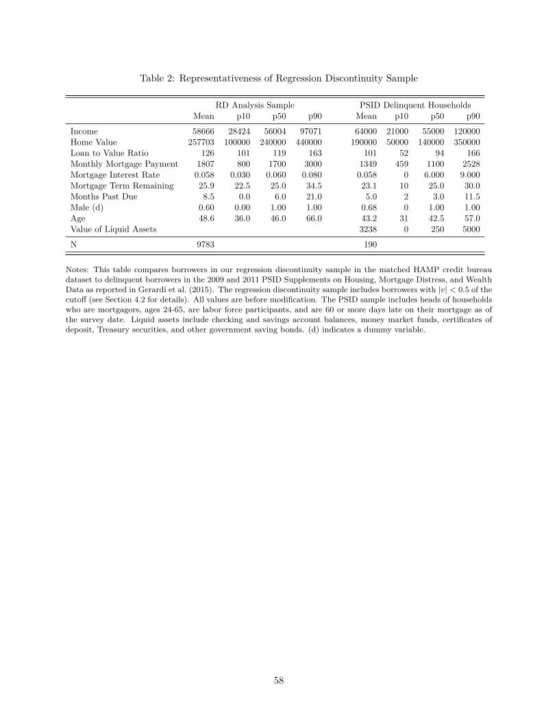
Table 2: Representativeness of Regression Discontinuity Sample

RD Analysis Sample PSID Delinquent HouseholdsMean p10 p50 p90 Mean p10 p50 p90

Income 58666 28424 56004 97071 64000 21000 55000 120000Home Value 257703 100000 240000 440000 190000 50000 140000 350000Loan to Value Ratio 126 101 119 163 101 52 94 166Monthly Mortgage Payment 1807 800 1700 3000 1349 459 1100 2528Mortgage Interest Rate 0.058 0.030 0.060 0.080 0.058 0 6.000 9.000Mortgage Term Remaining 25.9 22.5 25.0 34.5 23.1 10 25.0 30.0Months Past Due 8.5 0.0 6.0 21.0 5.0 2 3.0 11.5Male (d) 0.60 0.00 1.00 1.00 0.68 0 1.00 1.00Age 48.6 36.0 46.0 66.0 43.2 31 42.5 57.0Value of Liquid Assets 3238 0 250 5000

N 9783 190

Notes: This table compares borrowers in our regression discontinuity sample in the matched HAMP credit bureaudataset to delinquent borrowers in the 2009 and 2011 PSID Supplements on Housing, Mortgage Distress, and WealthData as reported in Gerardi et al. (2015). The regression discontinuity sample includes borrowers with |v| < 0.5 of thecutoff (see Section 4.2 for details). All values are before modification. The PSID sample includes heads of householdswho are mortgagors, ages 24-65, are labor force participants, and are 60 or more days late on their mortgage as ofthe survey date. Liquid assets include checking and savings account balances, money market funds, certificates ofdeposit, Treasury securities, and other government saving bonds. (d) indicates a dummy variable.

58

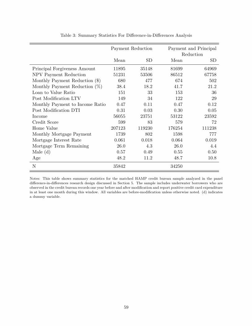
Table 3: Summary Statistics For Difference-in-Differences Analysis

Payment Reduction Payment and PrincipalReduction

Mean SD Mean SD

Principal Forgiveness Amount 11895 35148 81699 64969NPV Payment Reduction 51231 53506 86512 67758Monthly Payment Reduction ($) 680 477 674 502Monthly Payment Reduction (%) 38.4 18.2 41.7 21.2Loan to Value Ratio 151 33 153 36Post Modification LTV 149 34 122 29Monthly Payment to Income Ratio 0.47 0.11 0.47 0.12Post Modification DTI 0.31 0.03 0.30 0.05Income 56055 23751 53122 23592Credit Score 599 83 579 72Home Value 207123 119230 176254 111238Monthly Mortgage Payment 1739 802 1598 777Mortgage Interest Rate 0.061 0.018 0.064 0.019Mortgage Term Remaining 26.0 4.3 26.0 4.4Male (d) 0.57 0.49 0.55 0.50Age 48.2 11.2 48.7 10.8

N 35842 34250

Notes: This table shows summary statistics for the matched HAMP credit bureau sample analyzed in the paneldifference-in-differences research design discussed in Section 5. The sample includes underwater borrowers who areobserved in the credit bureau records one year before and after modification and report positive credit card expenditurein at least one month during this window. All variables are before-modification unless otherwise noted. (d) indicatesa dummy variable.

59

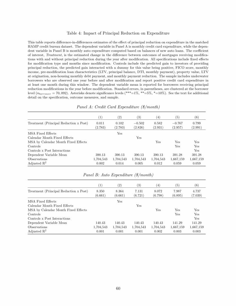
Table 4: Impact of Principal Reduction on Expenditure

This table reports difference-in-differences estimates of the effect of principal reduction on expenditure in the matchedHAMP credit bureau dataset. The dependent variable in Panel A is monthly credit card expenditure, while the depen-dent variable in Panel B is monthly auto expenditure computed based on balances of new auto loans. The coefficientof interest, Treatment, is the estimated change in the difference between outcomes of mortgages receiving modifica-tions with and without principal reduction during the year after modification. All specifications include fixed effectsfor modification type and months since modification. Controls include the predicted gain to investors of providingprincipal reduction, the predicted gain interacted with a dummy for this value being positive, FICO score, monthlyincome, pre-modification loan characteristics (LTV, principal balance, DTI, monthly payment), property value, LTVat origination, non-housing monthly debt payment, and monthly payment reduction. The sample includes underwaterborrowers who are observed one year before and after modification and report positive credit card expenditure inat least one month during this window. The dependent variable mean is reported for borrowers receiving principalreduction modifications in the year before modification. Standard errors, in parentheses, are clustered at the borrowerlevel (nborrower = 70, 092). Asterisks denote significance levels (***=1%, **=5%, *=10%). See the text for additionaldetail on the specification, outcome measures, and sample.

Panel A: Credit Card Expenditure ($/month)

(1) (2) (3) (4) (5) (6)

Treatment (Principal Reduction x Post) 0.011 0.102 −0.502 0.582 −0.767 0.799(2.783) (2.783) (2.826) (2.931) (2.957) (2.991)

MSA Fixed Effects YesCalendar Month Fixed Effects YesMSA by Calendar Month Fixed Effects Yes Yes YesControls Yes YesControls x Post Interactions YesDependent Variable Mean 390.13 390.13 390.13 390.13 391.28 391.28Observations 1,704,543 1,704,543 1,704,543 1,704,543 1,667,159 1,667,159Adjusted R2 0.002 0.014 0.005 0.012 0.059 0.059

Panel B: Auto Expenditure ($/month)

(1) (2) (3) (4) (5) (6)

Treatment (Principal Reduction x Post) 8.350 8.364 7.131 8.072 7.987 4.737(6.661) (6.661) (6.721) (6.798) (6.895) (7.039)

MSA Fixed Effects YesCalendar Month Fixed Effects YesMSA by Calendar Month Fixed Effects Yes Yes YesControls Yes YesControls x Post Interactions YesDependent Variable Mean 140.43 140.43 140.43 140.43 141.29 141.29Observations 1,704,543 1,704,543 1,704,543 1,704,543 1,667,159 1,667,159Adjusted R2 0.001 0.001 0.001 0.002 0.003 0.003

60

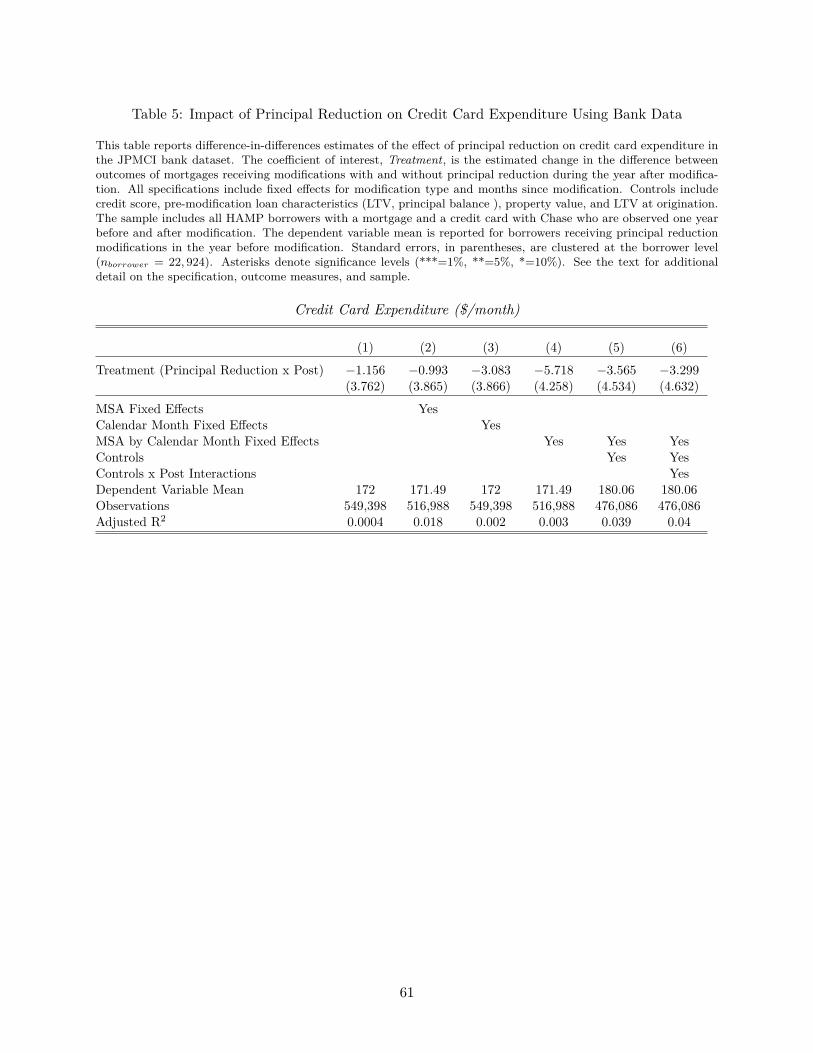
Table 5: Impact of Principal Reduction on Credit Card Expenditure Using Bank Data

This table reports difference-in-differences estimates of the effect of principal reduction on credit card expenditure inthe JPMCI bank dataset. The coefficient of interest, Treatment, is the estimated change in the difference betweenoutcomes of mortgages receiving modifications with and without principal reduction during the year after modifica-tion. All specifications include fixed effects for modification type and months since modification. Controls includecredit score, pre-modification loan characteristics (LTV, principal balance ), property value, and LTV at origination.The sample includes all HAMP borrowers with a mortgage and a credit card with Chase who are observed one yearbefore and after modification. The dependent variable mean is reported for borrowers receiving principal reductionmodifications in the year before modification. Standard errors, in parentheses, are clustered at the borrower level(nborrower = 22, 924). Asterisks denote significance levels (***=1%, **=5%, *=10%). See the text for additionaldetail on the specification, outcome measures, and sample.

Credit Card Expenditure ($/month)

(1) (2) (3) (4) (5) (6)

Treatment (Principal Reduction x Post) −1.156 −0.993 −3.083 −5.718 −3.565 −3.299(3.762) (3.865) (3.866) (4.258) (4.534) (4.632)

MSA Fixed Effects YesCalendar Month Fixed Effects YesMSA by Calendar Month Fixed Effects Yes Yes YesControls Yes YesControls x Post Interactions YesDependent Variable Mean 172 171.49 172 171.49 180.06 180.06Observations 549,398 516,988 549,398 516,988 476,086 476,086Adjusted R2 0.0004 0.018 0.002 0.003 0.039 0.04

61

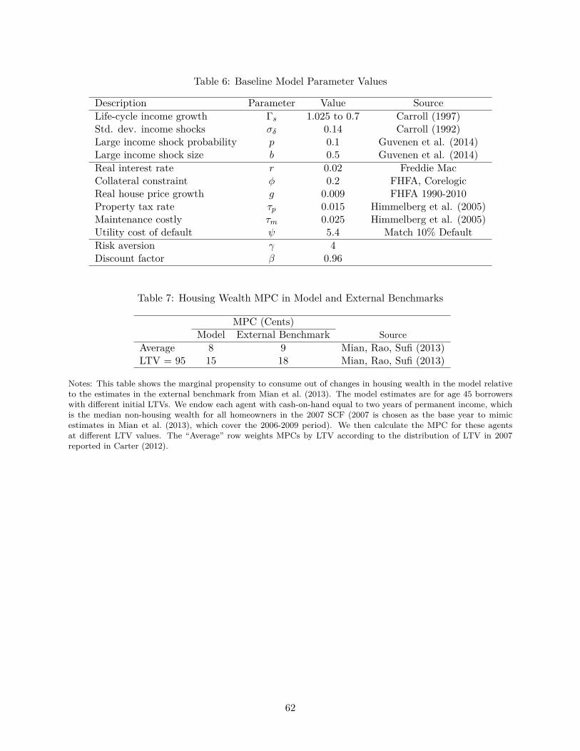
Table 6: Baseline Model Parameter Values

Description Parameter Value SourceLife-cycle income growth Γs 1.025 to 0.7 Carroll (1997)Std. dev. income shocks σδ 0.14 Carroll (1992)Large income shock probability p 0.1 Guvenen et al. (2014)Large income shock size b 0.5 Guvenen et al. (2014)Real interest rate r 0.02 Freddie MacCollateral constraint φ 0.2 FHFA, CorelogicReal house price growth g 0.009 FHFA 1990-2010Property tax rate τp 0.015 Himmelberg et al. (2005)Maintenance costly τm 0.025 Himmelberg et al. (2005)Utility cost of default ψ 5.4 Match 10% DefaultRisk aversion γ 4Discount factor β 0.96

Table 7: Housing Wealth MPC in Model and External Benchmarks

MPC (Cents)Model External Benchmark Source

Average 8 9 Mian, Rao, Sufi (2013)LTV = 95 15 18 Mian, Rao, Sufi (2013)

Notes: This table shows the marginal propensity to consume out of changes in housing wealth in the model relativeto the estimates in the external benchmark from Mian et al. (2013). The model estimates are for age 45 borrowerswith different initial LTVs. We endow each agent with cash-on-hand equal to two years of permanent income, whichis the median non-housing wealth for all homeowners in the 2007 SCF (2007 is chosen as the base year to mimicestimates in Mian et al. (2013), which cover the 2006-2009 period). We then calculate the MPC for these agentsat different LTV values. The “Average” row weights MPCs by LTV according to the distribution of LTV in 2007reported in Carter (2012).

62

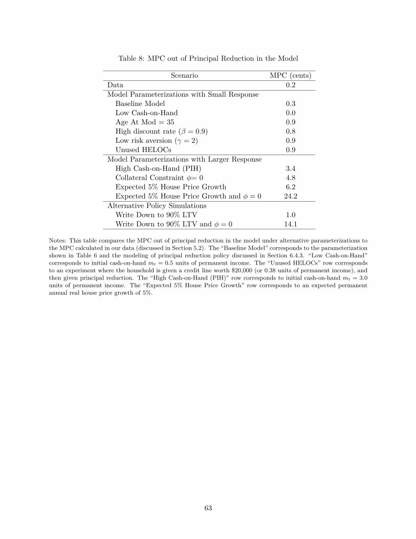
Table 8: MPC out of Principal Reduction in the Model

Scenario MPC (cents)Data 0.2Model Parameterizations with Small Response

Baseline Model 0.3Low Cash-on-Hand 0.0Age At Mod = 35 0.9High discount rate (β = 0.9) 0.8Low risk aversion (γ = 2) 0.9Unused HELOCs 0.9

Model Parameterizations with Larger ResponseHigh Cash-on-Hand (PIH) 3.4Collateral Constraint φ= 0 4.8Expected 5% House Price Growth 6.2Expected 5% House Price Growth and φ = 0 24.2

Alternative Policy SimulationsWrite Down to 90% LTV 1.0Write Down to 90% LTV and φ = 0 14.1

Notes: This table compares the MPC out of principal reduction in the model under alternative parameterizations tothe MPC calculated in our data (discussed in Section 5.2). The “Baseline Model” corresponds to the parameterizationshown in Table 6 and the modeling of principal reduction policy discussed in Section 6.4.3. “Low Cash-on-Hand”corresponds to initial cash-on-hand mt = 0.5 units of permanent income. The “Unused HELOCs” row correspondsto an experiment where the household is given a credit line worth $20,000 (or 0.38 units of permanent income), andthen given principal reduction. The “High Cash-on-Hand (PIH)” row corresponds to initial cash-on-hand mt = 3.0units of permanent income. The “Expected 5% House Price Growth” row corresponds to an expected permanentannual real house price growth of 5%.

63

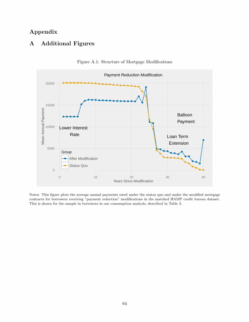
Appendix

A Additional Figures

Figure A.1: Structure of Mortgage Modifications

● ● ● ● ●

●

●● ● ● ● ● ● ● ● ● ● ● ● ● ●

●

●

●

●●

● ●● ●

● ● ●●

● ●

● ●●

●

Lower Interest

Rate Loan Term

Extension

Balloon

Payment

0

5000

10000

15000

20000

0 10 20 30 40Years Since Modification

Mea

n A

nnua

l Pay

men

t

Group

● After Modification

Status Quo

Payment Reduction Modification

Notes: This figure plots the average annual payments owed under the status quo and under the modified mortgagecontracts for borrowers receiving “payment reduction” modifications in the matched HAMP credit bureau dataset.This is shown for the sample in borrowers in our consumption analysis, described in Table 3.

64

Figure A.2: Modification Terms Summary

Notes: This figure shows the modified payment terms as explained to borrowers in the modification agreement whichthey are required to sign. Example terms are shown for a mortgage with a post-modification principal balance of$300,00, temporary interest rate of 2%, mortgage term of 35 years, and escrow payments equal to 1.5% of the propertyvalue ($250,000).

65

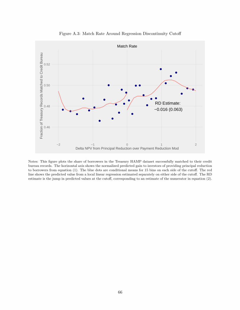
Figure A.3: Match Rate Around Regression Discontinuity Cutoff

●●

●

●

●

●

●

●

●

●

●

●

●

●

●

●

●

● ●

●

●

● ●

●

●

●

●

●

●●

RD Estimate:

−0.016 (0.063)

0.46

0.48

0.50

0.52

−2 −1 0 1 2Delta NPV from Principal Reduction over Payment Reduction Mod

Fra

ctio

n of

Tre

asur

y R

ecor

ds M

atch

ed to

Cre

dit B

urea

u

Match Rate

Notes: This figure plots the share of borrowers in the Treasury HAMP dataset successfully matched to their creditbureau records. The horizontal axis shows the normalized predicted gain to investors of providing principal reductionto borrowers from equation (1). The blue dots are conditional means for 15 bins on each side of the cutoff. The redline shows the predicted value from a local linear regression estimated separately on either side of the cutoff. The RDestimate is the jump in predicted values at the cutoff, corresponding to an estimate of the numerator in equation (2).

66

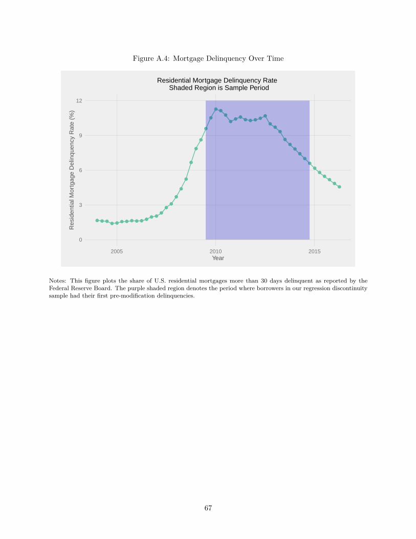
Figure A.4: Mortgage Delinquency Over Time

● ● ●● ● ● ● ● ● ● ●

● ●●

●●

●

●

●

●

●

●

●

●

● ●●

●●

●● ● ● ●

●

●●

●

●

●

●

●

●

●

●●

●●

●●

0

3

6

9

12

2005 2010 2015Year

Res

iden

tial M

ortg

age

Del

inqu

ency

Rat

e (%

)

Residential Mortgage Delinquency Rate Shaded Region is Sample Period

Notes: This figure plots the share of U.S. residential mortgages more than 30 days delinquent as reported by theFederal Reserve Board. The purple shaded region denotes the period where borrowers in our regression discontinuitysample had their first pre-modification delinquencies.

67

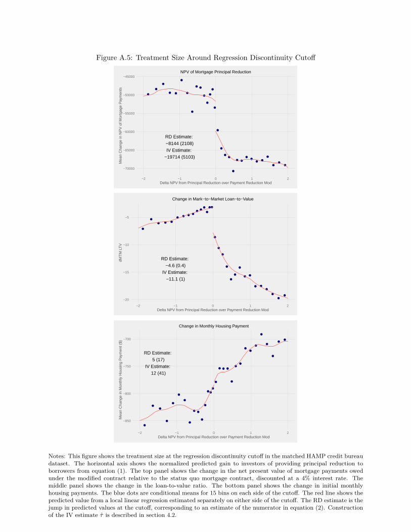
Figure A.5: Treatment Size Around Regression Discontinuity Cutoff

●

●

●

● ●

●

●

●

●●

●

●

●

●

●

●

●

●●

●

● ●

●●

●●

●

●●

●

RD Estimate:

−8144 (2108)

IV Estimate:

−19714 (5103)

−70000

−65000

−60000

−55000

−50000

−45000

−2 −1 0 1 2Delta NPV from Principal Reduction over Payment Reduction Mod

Mea

n C

hang

e in

NP

V o

f Mor

tgag

e P

aym

ents

NPV of Mortgage Principal Reduction

●

●

● ● ●

●● ●

●

●●

●

●

● ●

●

●

●

●

●

●

●

● ●

● ●

●

●

●

●

RD Estimate:

−4.6 (0.4)

IV Estimate:

−11.1 (1)

−20

−15

−10

−5

−2 −1 0 1 2Delta NPV from Principal Reduction over Payment Reduction Mod

dMT

M L

TV

Change in Mark−to−Market Loan−to−Value

●

●

●

●

●

●

●

●

●●

●

●

● ●

●

●

● ● ●

●

●●

●●

●

●

●

●

●●

RD Estimate:

5 (17)

IV Estimate:

12 (41)

−850

−800

−750

−700

−2 −1 0 1 2Delta NPV from Principal Reduction over Payment Reduction Mod

Mea

n C

hang

e in

Mon

thly

Hou

sing

Pay

men

t ($)

Change in Monthly Housing Payment

Notes: This figure shows the treatment size at the regression discontinuity cutoff in the matched HAMP credit bureaudataset. The horizontal axis shows the normalized predicted gain to investors of providing principal reduction toborrowers from equation (1). The top panel shows the change in the net present value of mortgage payments owedunder the modified contract relative to the status quo mortgage contract, discounted at a 4% interest rate. Themiddle panel shows the change in the loan-to-value ratio. The bottom panel shows the change in initial monthlyhousing payments. The blue dots are conditional means for 15 bins on each side of the cutoff. The red line shows thepredicted value from a local linear regression estimated separately on either side of the cutoff. The RD estimate is thejump in predicted values at the cutoff, corresponding to an estimate of the numerator in equation (2). Constructionof the IV estimate τ̂ is described in section 4.2.

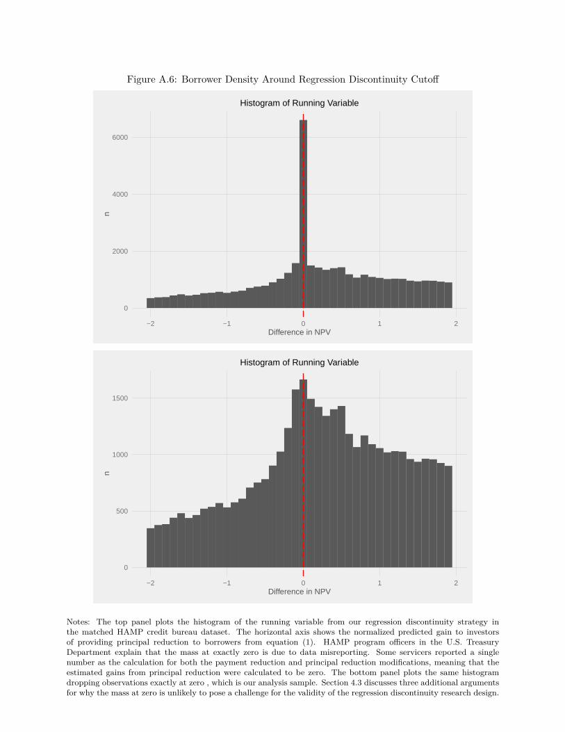
Figure A.6: Borrower Density Around Regression Discontinuity Cutoff

0

2000

4000

6000

−2 −1 0 1 2Difference in NPV

nHistogram of Running Variable

0

500

1000

1500

−2 −1 0 1 2Difference in NPV

n

Histogram of Running Variable

Notes: The top panel plots the histogram of the running variable from our regression discontinuity strategy inthe matched HAMP credit bureau dataset. The horizontal axis shows the normalized predicted gain to investorsof providing principal reduction to borrowers from equation (1). HAMP program officers in the U.S. TreasuryDepartment explain that the mass at exactly zero is due to data misreporting. Some servicers reported a singlenumber as the calculation for both the payment reduction and principal reduction modifications, meaning that theestimated gains from principal reduction were calculated to be zero. The bottom panel plots the same histogramdropping observations exactly at zero , which is our analysis sample. Section 4.3 discusses three additional argumentsfor why the mass at zero is unlikely to pose a challenge for the validity of the regression discontinuity research design.

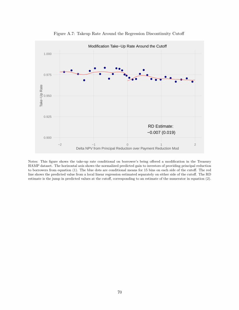
Figure A.7: Takeup Rate Around the Regression Discontinuity Cutoff

●●

●

●

●

●

●

●

●

●

● ●●

●●

●● ●

●

●

●

● ● ●

●●

●●

●

●

RD Estimate: −0.007 (0.019)

0.900

0.925

0.950

0.975

1.000

−2 −1 0 1 2Delta NPV from Principal Reduction over Payment Reduction Mod

Take

−U

p R

ate

Modification Take−Up Rate Around the Cutoff

Notes: This figure shows the take-up rate conditional on borrower’s being offered a modification in the TreasuryHAMP dataset. The horizontal axis shows the normalized predicted gain to investors of providing principal reductionto borrowers from equation (1). The blue dots are conditional means for 15 bins on each side of the cutoff. The redline shows the predicted value from a local linear regression estimated separately on either side of the cutoff. The RDestimate is the jump in predicted values at the cutoff, corresponding to an estimate of the numerator in equation (2).

70

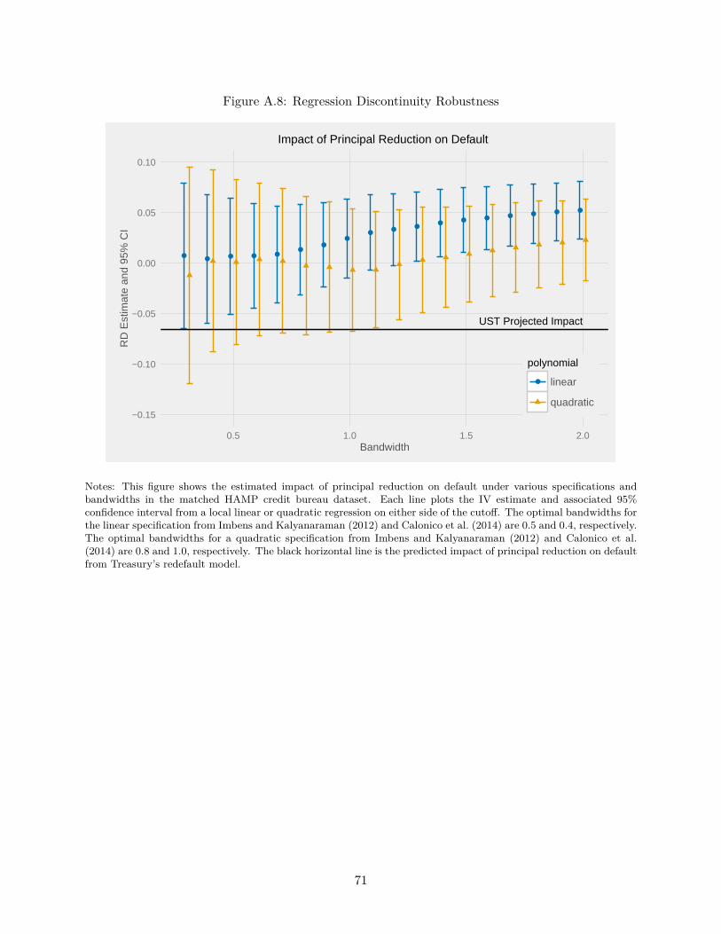
Figure A.8: Regression Discontinuity Robustness

●● ● ● ●

●●

●●

● ●● ● ● ● ● ● ●

UST Projected Impact

−0.15

−0.10

−0.05

0.00

0.05

0.10

0.5 1.0 1.5 2.0Bandwidth

RD

Est

imat

e an

d 95

% C

I

polynomial

● linear

quadratic

Impact of Principal Reduction on Default

Notes: This figure shows the estimated impact of principal reduction on default under various specifications andbandwidths in the matched HAMP credit bureau dataset. Each line plots the IV estimate and associated 95%confidence interval from a local linear or quadratic regression on either side of the cutoff. The optimal bandwidths forthe linear specification from Imbens and Kalyanaraman (2012) and Calonico et al. (2014) are 0.5 and 0.4, respectively.The optimal bandwidths for a quadratic specification from Imbens and Kalyanaraman (2012) and Calonico et al.(2014) are 0.8 and 1.0, respectively. The black horizontal line is the predicted impact of principal reduction on defaultfrom Treasury’s redefault model.

71

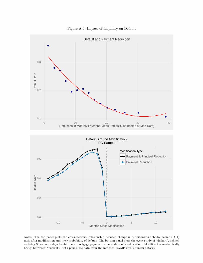
Figure A.9: Impact of Liquidity on Default

●

●

●

●●

●

●

●

●

●●

● ●

●

●

0.1

0.2

0.3

0 10 20 30 40Reduction in Monthly Payment (Measured as % of Income at Mod Date)

Def

ault

Rat

e

Default and Payment Reduction

●

●

●

●

●●

●

●

●●

●

●

● ● ● ● ● ● ● ● ● ● ● ● ●

0.0

0.2

0.4

0.6

−10 −5 0 5 10Months Since Modification

Def

ault

Rat

e

Modification Type

● Payment & Principal Reduction

Payment Reduction

Default Around Modification RD Sample

Notes: The top panel plots the cross-sectional relationship between change in a borrower’s debt-to-income (DTI)ratio after modification and their probability of default. The bottom panel plots the event study of “default”, definedas being 90 or more days behind on a mortgage payment, around date of modification. Modification mechanicallybrings borrowers “current”. Both panels use data from the matched HAMP credit bureau dataset.

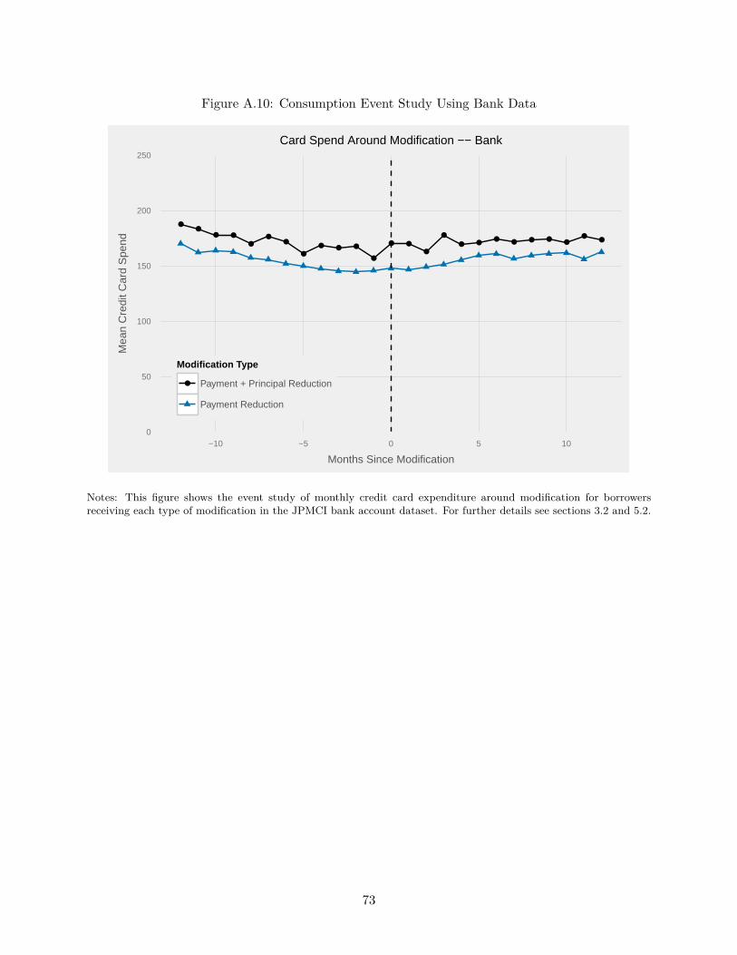
Figure A.10: Consumption Event Study Using Bank Data

●●

● ●

●●

●

●● ● ●

●

● ●●

●

● ●● ● ● ● ●

●●

0

50

100

150

200

250

−10 −5 0 5 10

Months Since Modification

Mea

n C

redi

t Car

d S

pend

Modification Type

● Payment + Principal Reduction

Payment Reduction

Card Spend Around Modification −− Bank

Notes: This figure shows the event study of monthly credit card expenditure around modification for borrowersreceiving each type of modification in the JPMCI bank account dataset. For further details see sections 3.2 and 5.2.

73

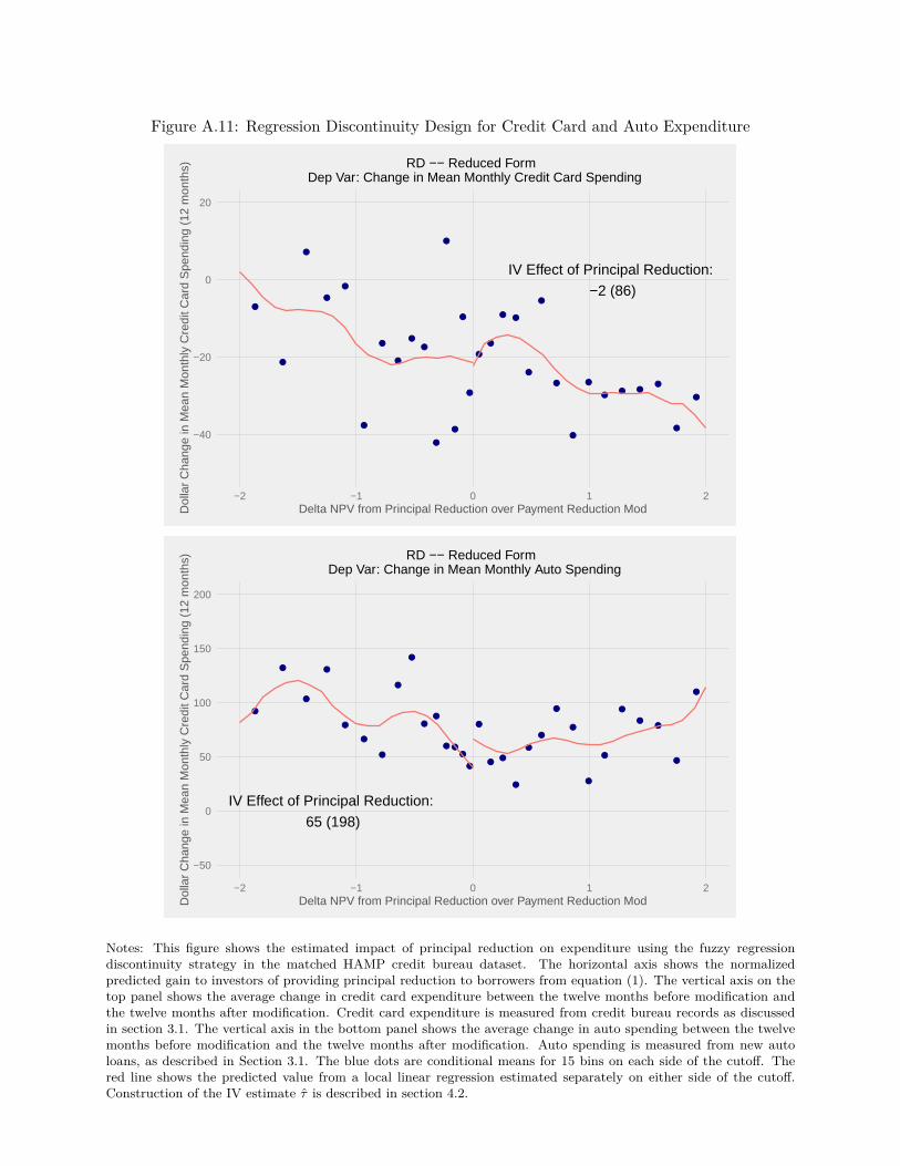
Figure A.11: Regression Discontinuity Design for Credit Card and Auto Expenditure

●

●

●

●

●

●

●

●

●●

●

●

●

●

●

●

●

● ●

●

●

●

●

●

●● ●

●

●

●

IV Effect of Principal Reduction: −2 (86)

−40

−20

0

20

−2 −1 0 1 2Delta NPV from Principal Reduction over Payment Reduction ModD

olla

r C

hang

e in

Mea

n M

onth

ly C

redi

t Car

d S

pend

ing

(12

mon

ths) RD −− Reduced Form

Dep Var: Change in Mean Monthly Credit Card Spending

●

●

●

●

●

●

●

●

●

●●

● ●●

●

●

●●

●

●

●

●

●

●

●

●

●●

●

●

IV Effect of Principal Reduction: 65 (198)

−50

0

50

100

150

200

−2 −1 0 1 2Delta NPV from Principal Reduction over Payment Reduction ModD

olla

r C

hang

e in

Mea

n M

onth

ly C

redi

t Car

d S

pend

ing

(12

mon

ths) RD −− Reduced Form

Dep Var: Change in Mean Monthly Auto Spending

Notes: This figure shows the estimated impact of principal reduction on expenditure using the fuzzy regressiondiscontinuity strategy in the matched HAMP credit bureau dataset. The horizontal axis shows the normalizedpredicted gain to investors of providing principal reduction to borrowers from equation (1). The vertical axis on thetop panel shows the average change in credit card expenditure between the twelve months before modification andthe twelve months after modification. Credit card expenditure is measured from credit bureau records as discussedin section 3.1. The vertical axis in the bottom panel shows the average change in auto spending between the twelvemonths before modification and the twelve months after modification. Auto spending is measured from new autoloans, as described in Section 3.1. The blue dots are conditional means for 15 bins on each side of the cutoff. Thered line shows the predicted value from a local linear regression estimated separately on either side of the cutoff.Construction of the IV estimate τ̂ is described in section 4.2.

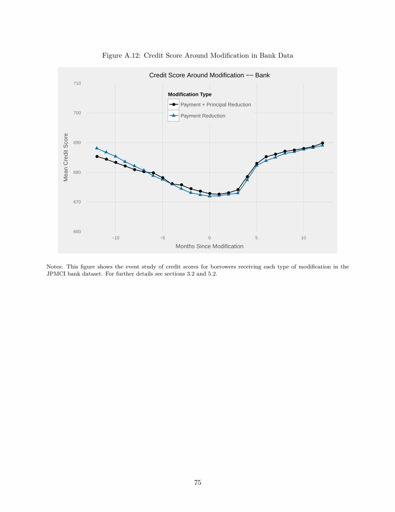
Figure A.12: Credit Score Around Modification in Bank Data

●●

●●

●● ●

●

● ●●

●● ● ●

●

●

●

●●

● ● ●●

●

660

670

680

690

700

710

−10 −5 0 5 10

Months Since Modification

Mea

n C

redi

t Sco

re

Modification Type

● Payment + Principal Reduction

Payment Reduction

Credit Score Around Modification −− Bank

Notes: This figure shows the event study of credit scores for borrowers receiving each type of modification in theJPMCI bank dataset. For further details see sections 3.2 and 5.2.

75

Figure A.13: Mortgage Credit Availability

● ● ●● ● ● ● ● ● ● ● ● ●

● ●● ●

●● ● ● ●

● ● ●● ● ●

●●

●

●

●

●

●●

●● ● ● ● ● ● ● ● ● ● ● ● ● ● ● ● ● ● ● ● ● ● ● ● ● ●

0.0

0.5

1.0

1.5

2.0

00:Q1 05:Q1 10:Q1 15:Q1Date

Rat

io to

200

7 Q

1

Credit Score ● < 620 620−659 660−719 720−779 780+

Mortgage Originations by Credit Score 4−Quarter Moving Average

●●

●●

●

● ●

●

●

●

●●

● ●

●●

60

65

70

75

2000 2005 2010 2015Year

CLT

V

Average CLTV Of HELOC Originations

Notes: The top panel plots mortgage origination by borrower credit score from the New York Fed Consumer CreditPanel (Federal Reserve 2015). This includes first mortgages, second mortgages, and home equity installment loans.The bottom panel plots the average combined loan-to-value (CLTV) ratio for new home equity lines of credit (HE-LOCs) as reported by Corelogic (2016).

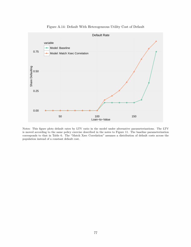
Figure A.14: Default With Heterogeneous Utility Cost of Default

● ● ● ● ● ● ● ●

● ● ● ● ●

●

●

●

0.00

0.25

0.50

0.75

50 100 150Loan−to−Value

Sha

re D

efau

lting

variable

● Model: Baseline

Model: Match Xsec Correlation

Default Rate

Notes: This figure plots default rates by LTV ratio in the model under alternative parameterizations. The LTVis moved according to the same policy exercise described in the notes to Figure 11. The baseline parameterizationcorresponds to that in Table 6. The “Match Xsec Correlation” assumes a distribution of default costs across thepopulation instead of a constant default cost.

77

B Effect of Payment Reduction on Default

In this section we analyze the effect of payment reduction on borrower default. Using a regres-sion discontinuity empirical strategy, we find that immediate payment reduction with no changein long-term obligations significantly reduces default. Our findings indicate that additional pay-ment reduction is effective irrespective of a borrower’s payment-to-income ratio, which is contraryto the view of affordability that has defined government housing policy since 1937. Furthermore,our findings suggest that the arbitrary income-ratio target embodied in the government programcrowded out private bilateral modifications that could have been more generous, and led to fewerdefaults, for up to 40% of HAMP borrowers. Finally, we show that by extending mortgage ma-turities, modifications can be structured so as to reduce defaults in a way that is likely to leaveborrowers, investors, and taxpayers better off.

B.1 Variation in Payment Reduction Between HAMP and Chase Modifications

We analyze the effect of immediate payment reduction by comparing borrowers with HAMPmodifications to those with proprietary modifications offered by Chase. Although servicers wererequired to offer all eligible borrowers HAMP modifications, HAMP had strict eligibility rules as de-scribed in section 2.1. Borrowers ineligible for HAMP were often eligible for alternative proprietarymodification programs offered by their servicer. We focus in particular on proprietary modificationsoffered by Chase. This section discusses two important features of the Chase modification programwhich allow us to carefully study the effect of modifications that reduce immediate payments with-out reducing long-term obligations, while the next section describes the specific HAMP eligibilityrule we rely on in our empirical strategy.

The design of HAMP and the Chase modification program reflect different views about the mosteffective way to reduce defaults. HAMP was designed with an explicit 31% payment-to-income(PTI) ratio target. This income ratio target evolved from the National Housing Act of 1937, whichestablished a PTI limit in the federal government’s public housing program (Schwartz and Wilson2008). Over the subsequent 80 years, the target spread throughout federal housing policies, firstin the rental market, then in the owner-occupied market, and finally in the design of mortgagemodifications during the Great Recession. Adopting this income ratio target in a modificationprogram assumes that borrowers with high PTI ratios must need much larger payment reductionsin order to avoid default than borrowers with lower PTI ratios, and that borrowers with PTI ratiosbelow 31% already have “affordable” mortgages and hence do not need assistance to avoid default.

The first important feature of the Chase modification program is that, in contrast to the rigidincome ratio target in HAMP, Chase joined a wide range of servicers and investors in the housingmarket (including Fannie Mae and Freddie Mac) in pursuing a strategy which added a payment-reduction target.51 Under this alternative view, the amount of payment reduction relative to thestatus quo is at least as important for reducing defaults as ensuring that the new payment is

51For more detail about the evolution of different modification strategies, see Cowley (2017).

81

an “affordable” share of income according to the government’s metric. Reflecting this view, theChase program mimics HAMP in modifying loans such that new payments hit the 31% PTI target,but adds the stipulation that if this results in a payment reduction of less than 30%, that themodification instead targets a 30% payment reduction.52 Under this rule, Chase modificationsresult in immediate payment reductions that are at least as great as in HAMP, and greater forborrowers with low PTI ratios who are either ineligible for HAMP or receive less than 30% paymentreductions in HAMP.

The second important feature of the Chase modification program is that maturity extensionwas used as a low-cost tool for achieving deeper immediate payment reductions without reducinglong-term obligations. A range of contract terms can be modified in order to achieve a given amountof immediate payment reduction. As described in section 2.1, HAMP reduced payments by firstproviding interest rate reductions, then maturity extensions, and finally principal forbearance asnecessary to achieve the 31% PTI ratio target. In contrast, Chase modifications targeted largerpayment reductions by first extending maturity and amortization terms (which we call maturity ex-tension for simplicity).53 In this way deeper immediate payment reductions are offset by continuedpayments in the long-term. The structure of Chase modifications can be seen visually in AppendixFigure B.3, which shows the average path of payments owed before and after modification.54 Lowpayments are sustained throughout the early mortgage term (since few borrowers have interestrates re-setting from temporary reductions), and continue for up to 40 years (since many borrowershave extended maturities). We compare cash-flows for various modification groups in more detailin section B.3.

B.2 31% Payment-to-Income Regression Discontinuity Empirical Strategy

Our strategy to identify the effect of immediate payment reduction on default uses variationgenerated by HAMP’s 31% PTI eligibility cutoff and the different payment reduction targets usedin HAMP and the Chase modification program. Since HAMP was designed to reduce monthlypayments to 31% of a borrower’s income, borrowers whose PTI ratio was already below 31% wereineligible for HAMP. These borrowers were only evaluated for Chase’s proprietary modificationprogram.

The difference in modification program rules generates substantial variation in the amount of52The Chase program specifically targets a 25% reduction in principal, interest, taxes, and insurance (PITI) pay-

ments, which translates to a 30% principal and interest reduction for most borrowers. We follow the convention inthe prior literature and characterize the reductions relative to prior principal and interest payments.

53Our language follows prior work by ? who discuss maturity choices in the auto loan market in a context whereamortization and maturity terms are equivalent. In both HAMP and the Chase modification program servicersextended mortgage maturities and re-amortized the mortgage to the new term, unless either step was prohibitedby investor agreements (in which case only the permitted step, if any, was pursued). In theoretical work analyzingconsumer debt restructuring policies ? use “maturity extension” to mean something different. They consider amodification with interest-only payments for a number of periods, with a corresponding increase in loan maturityand no change in the amortization schedule during the periods when principal payments are made.

54While the HAMP program ended in December 2016, the Chase modification program described in this sectionis ongoing and its rules are subject to change. Our description of the program reflects guidelines in place during ouranalysis period.

82

immediate payment reduction received by borrowers on either side of HAMP’s 31% PTI eligibilitycutoff. Above the cutoff borrowers receive a mix of HAMP modifications with small payment reduc-tions (since these borrowers are already close to HAMP’s 31% PTI target) and Chase modificationswith large payment reductions (since Chase had a minimum 30% payment reduction target). Belowthe cutoff, all borrowers receive Chase modifications with large payment reductions. The result isthat the average payment reduction jumps sharply at the cutoff.

Employing a fuzzy regression discontinuity strategy, the treatment effect of receiving paymentreduction is determined by the jump in default divided by the jump in the amount of paymentreduction received at the cutoff. Similar to equation 2, let Y be the outcome variable of interest,and let ∆Pay be the percent change in mortgage payment from the modification. The estimandfor the effect of a 1% payment reduction is given by

τ =limPTI↓31%E[Y |PTI]− limPTI↑31%E[Y |PTI]

limPTI↓31%E[∆Pay|PTI]− limPTI↑31%E[∆Pay|PTI] . (7)

We follow the procedures described in section 4.2 to estimate τ̂ using borrowers in the JPMCIbank dataset. The full sample includes all non-GSE borrowers who received a modification througheither the HAMP or Chase programs. We further limit the sample to modifications performed inthe fourth quarter of 2011 or later, and who are observed at least two years after modification. TheChase proprietary program we study was instituted after HAMP was in place, and by the fourthquarter of 2011 it was sufficiently established such that any borrower ineligible for HAMP due tothe PTI cutoff could plausibly receive a Chase modification.55 The sample includes borrowers withPTI ratios between 25 and 80.56 For symmetry around the 31% PTI cutoff, most figures in thefollowing sections plot data for borrowers with PTI ratios between 25% and 37%. The optimalbandwidth according to the Imbens and Kalyanaraman (2012) procedure is 4.5 percentage pointsof PTI, though we report estimates for multiple bandwidths.

B.3 Internal Validity of Design

As with the investor NPV regression discontinuity strategy, the validity of this research designrests on two assumptions. First, there is a discontinuous jump in the amount of immediate pay-ment reduction received at the cutoff. Second, all other variables that could affect outcomes arecontinuous at the cutoff.

The top panel of Figure B.1 validates the first assumption. It shows that borrowers below thecutoff receive payment reductions that are 17.4 percentage points more generous than those receivedby borrowers above the cutoff.57 The figure also shows that payment reductions are approximately

55Chase had a variety of other modification programs with different designs that preceded HAMP.56Borrower density thins above PTI ratios of 80, and borrowers with PTI ratios below 25 are evaluated according

to different program rules.57This figure, and all subsequent figures in the section, remove the 275 observations with PTI ratios between 31%

and 31.1%. Borrowers this close to the cutoff receive an amount of payment reduction which is about halfway betweenthat received by borrowers clearly above and clearly below the cutoff. This can be seen in the top panel of AppendixFigure B.4. The bottom panel of this figure shows that the estimated effect of payment reduction on default is nearly

83

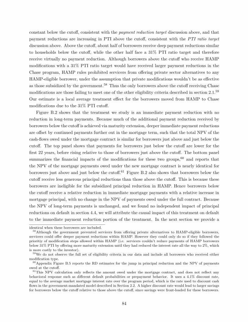
constant below the cutoff, consistent with the payment reduction target discussion above, and thatpayment reductions are increasing in PTI above the cutoff, consistent with the PTI ratio targetdiscussion above. Above the cutoff, about half of borrowers receive deep payment reductions similarto households below the cutoff, while the other half face a 31% PTI ratio target and thereforereceive virtually no payment reduction. Although borrowers above the cutoff who receive HAMPmodifications with a 31% PTI ratio target would have received larger payment reductions in theChase program, HAMP rules prohibited servicers from offering private sector alternatives to anyHAMP-eligible borrower, under the assumption that private modifications wouldn’t be as effectiveas those subsidized by the government.58 Thus the only borrowers above the cutoff receiving Chasemodifications are those failing to meet one of the other eligibility criteria described in section 2.1.59

Our estimate is a local average treatment effect for the borrowers moved from HAMP to Chasemodifications due to the 31% PTI cutoff.

Figure B.2 shows that the treatment we study is an immediate payment reduction with noreduction in long-term payments. Because much of the additional payment reduction received byborrowers below the cutoff is achieved via maturity extension, deeper immediate payment reductionsare offset by continued payments further out in the mortgage term, such that the total NPV of thecash-flows owed under the mortgage contract is similar for borrowers just above and just below thecutoff. The top panel shows that payments for borrowers just below the cutoff are lower for thefirst 22 years, before rising relative to those of borrowers just above the cutoff. The bottom panelsummarizes the financial impacts of the modifications for these two groups,60 and reports thatthe NPV of the mortgage payments owed under the new mortgage contract is nearly identical forborrowers just above and just below the cutoff.61 Figure B.2 also shows that borrowers below thecutoff receive less generous principal reductions than those above the cutoff. This is because theseborrowers are ineligible for the subsidized principal reduction in HAMP. Hence borrowers belowthe cutoff receive a relative reduction in immediate mortgage payments with a relative increase inmortgage principal, with no change in the NPV of payments owed under the full contract. Becausethe NPV of long-term payments is unchanged, and we found no independent impact of principalreductions on default in section 4.4, we will attribute the causal impact of this treatment on defaultto the immediate payment reduction portion of the treatment. In the next section we provide a

identical when these borrowers are included.58Although the government prevented servicers from offering private alternatives to HAMP-eligible borrowers,

servicers could offer deeper payment reductions within HAMP. However they could only do so if they followed theprioritiy of modification steps allowed within HAMP (i.e. servicers couldn’t reduce payments of HAMP borrowersbelow 31% PTI by offering more maturity extension until they had reduced the interest rate all the way to 2%, whichis more costly to the investor).

59We do not observe the full set of eligibility criteria in our data and include all borrowers who received eithermodification type.

60Appendix Figure B.5 reports the RD estimates for the jump in principal reduction and the NPV of paymentsowed at the cutoff.

61This NPV calculation only reflects the amount owed under the mortgage contract, and does not reflect anybehavioral response such as different default probabilities or prepayment behavior. It uses a 4.1% discount rate,equal to the average market mortgage interest rate over the program period, which is the rate used to discount cashflows in the government-mandated model described in Section 2.2. A higher discount rate would lead to larger savingsfor borrowers below the cutoff relative to those above the cutoff, since savings were front-loaded for these borrowers.

84

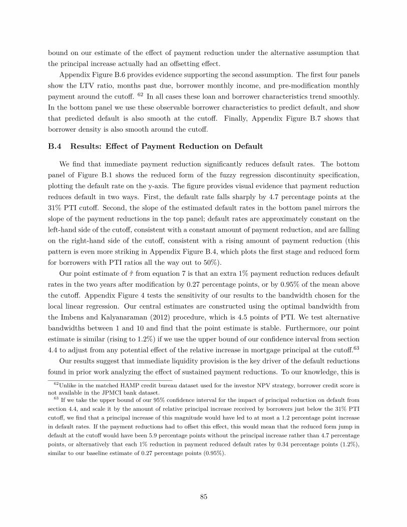
bound on our estimate of the effect of payment reduction under the alternative assumption thatthe principal increase actually had an offsetting effect.

Appendix Figure B.6 provides evidence supporting the second assumption. The first four panelsshow the LTV ratio, months past due, borrower monthly income, and pre-modification monthlypayment around the cutoff. 62 In all cases these loan and borrower characteristics trend smoothly.In the bottom panel we use these observable borrower characteristics to predict default, and showthat predicted default is also smooth at the cutoff. Finally, Appendix Figure B.7 shows thatborrower density is also smooth around the cutoff.

B.4 Results: Effect of Payment Reduction on Default

We find that immediate payment reduction significantly reduces default rates. The bottompanel of Figure B.1 shows the reduced form of the fuzzy regression discontinuity specification,plotting the default rate on the y-axis. The figure provides visual evidence that payment reductionreduces default in two ways. First, the default rate falls sharply by 4.7 percentage points at the31% PTI cutoff. Second, the slope of the estimated default rates in the bottom panel mirrors theslope of the payment reductions in the top panel; default rates are approximately constant on theleft-hand side of the cutoff, consistent with a constant amount of payment reduction, and are fallingon the right-hand side of the cutoff, consistent with a rising amount of payment reduction (thispattern is even more striking in Appendix Figure B.4, which plots the first stage and reduced formfor borrowers with PTI ratios all the way out to 50%).

Our point estimate of τ̂ from equation 7 is that an extra 1% payment reduction reduces defaultrates in the two years after modification by 0.27 percentage points, or by 0.95% of the mean abovethe cutoff. Appendix Figure 4 tests the sensitivity of our results to the bandwidth chosen for thelocal linear regression. Our central estimates are constructed using the optimal bandwidth fromthe Imbens and Kalyanaraman (2012) procedure, which is 4.5 points of PTI. We test alternativebandwidths between 1 and 10 and find that the point estimate is stable. Furthermore, our pointestimate is similar (rising to 1.2%) if we use the upper bound of our confidence interval from section4.4 to adjust from any potential effect of the relative increase in mortgage principal at the cutoff.63

Our results suggest that immediate liquidity provision is the key driver of the default reductionsfound in prior work analyzing the effect of sustained payment reductions. To our knowledge, this is

62Unlike in the matched HAMP credit bureau dataset used for the investor NPV strategy, borrower credit score isnot available in the JPMCI bank dataset.

63 If we take the upper bound of our 95% confidence interval for the impact of principal reduction on default fromsection 4.4, and scale it by the amount of relative principal increase received by borrowers just below the 31% PTIcutoff, we find that a principal increase of this magnitude would have led to at most a 1.2 percentage point increasein default rates. If the payment reductions had to offset this effect, this would mean that the reduced form jump indefault at the cutoff would have been 5.9 percentage points without the principal increase rather than 4.7 percentagepoints, or alternatively that each 1% reduction in payment reduced default rates by 0.34 percentage points (1.2%),similar to our baseline estimate of 0.27 percentage points (0.95%).

85

the first estimate of the effect of an immediate payment reduction with no reduction in long-termpayments. Our results are similar to two types of estimates in the prior literature which analyzessustained payment reductions. First, Agarwal et al. (2011) and Haughwout et al. (2016) analyzemodifications provided to delinquent borrowers before the implementation of the HAMP program.They find that a 1% immediate payment reduction that also reduces long-term debt obligations isassociated with a 1.1% to 1.3% reduction in default rates.64 Second, other authors have analyzedthe effect of sustained payment reductions for non-distressed borrowers. Although differences inborrower characteristics and baseline default rates makes it difficult to directly compare magnitudesbetween distressed and non-distressed borrowers, this literature has found that a 1% paymentreduction is associated with a 1.1% to 2.75% reduction in default rates.65 The similarity between ourestimates of the effect of immediate payment reduction and those of the prior literature analyzingthe effect of sustained payment reductions suggests that immediate liquidity provision is a maindriver of the default reductions documented in previous work.

B.5 Implications

Our finding that the type of payment reduction we study can substantially reduce defaults hasthree broader implications. This section discusses each implication in turn.

First, our findings reject the homogeneous-preferences view of housing affordability that hasbeen embodied in government housing policy since 1937. A one-size-fits-all PTI ratio target couldbe justified by a model where agents have Cobb-Douglas preferences over housing and non-housingconsumption and all have identical tastes for housing.66 Such a model predicts that all householdswill choose to spend the same share of their income on housing. Payments above this share wouldlead to defaults while payments below this share would be sustainable. With a 31% PTI target,this view implies that default rates should be converging to zero as average PTI approaches 31%.In contrast, we show that default rates are well above zero for households below this cutoff.

Instead, our results are more consistent with a model with heterogeneous tastes for housingwhere liquidity shocks are the main drivers of default. A model with heterogeneous preferences forhousing would suggest that different households have different preferred income shares of housing.

64In addition, Agarwal et al. (2016a) show that HAMP modifications with both short and long-term paymentreduction led to significant reductions in default rates, though they do not estimate an elasticity with respect to agiven quantity of payment reduction.

65See Ehrlich and Perry (2015), Tracy and Wright (2012), Fuster and Willen (2017), and DiMaggio et al. (2017).The latter three of these papers analyze the effect of payment reductions caused by downward adjustments of interestrates for borrowers with adjustable rate mortgages. As Fuster and Willen (2017) discuss, to the extent that borrowersare aware of their mortgage terms and follow the movement of underlying index rates, then these estimates may alreadybe capturing only the liquidity effects of lower payments since borrowers would already have been anticipating andresponding to the long-term payment reductions. Similarly, in contemporaneous work Scharlemann and Shore (2017)analyze the effect of sustained payment increases for non-distressed borrowers in a setting where these paymentincreases are pre-determined five years ahead of time (resulting from a step up in interest rates as part of a previousmortgage modification). They find that a 1% increase in payments is associated with a 0.8% reduction in defaultrates.

66An alternative justification specific to the owner-occupied market is the value of PTI limits from a macroprudentialpolicy perspective. Greenwald (2017) finds that a cap on PTI ratios is more effective than a cap on LTV ratios atlimiting boom-bust cycles.

86

Households could support a wide range of potential PTI ratios, but temporary income or expenseshocks would induce them to default even at potentially low PTI ratios. In these cases, a paymentreduction would plausibly allow them to maintain payments. Our empirical results are consistentboth with liquidity-shock driven defaults (section 4.6) and the effectiveness of payment reductionseven for low-PTI borrowers. We find that payment reductions led to a substantial reduction indefault rates, even for borrowers already at the 31% PTI ratio target who supposedly had “afford-able” mortgages according to the government’s rule. Furthermore, for borrowers above the 31%cutoff, those who started with higher PTI ratios and thus received more payment reduction hadlower default rates than those starting with lower PTI ratios, even though HAMP reduced the PTIratio of both groups to the same 31% target.

Second, our data showing that the government’s rigid income ratio target generated less generousmodifications than private sector alternatives, coupled with the government’s requirement thatborrowers be offered HAMP before private alternatives, raise concerns about substantial crowd-out which may have had the unintended effect of increasing defaults for up to 40% of HAMPborrowers. The 31% PTI target in HAMP means that borrowers with pre-modification PTI ratiosbelow 41.5% received payment reductions of less than 30%. For these borrowers, an alternativeprivate bilateral modification program such as the one we studied would have resulted in moregenerous immediate payment reduction and, according to our empirical results, lower default rateswithout requiring any government intervention or subsidy. About 40% of all borrowers with HAMPmodifications (625,000 borrowers) were in this region, and the government spent approximately$7 billion subsidizing potentially less effective modifications for these borrowers.67 Furthermore,the government explicitly prohibited servicers from offering alternative private modifications toany HAMP-eligible borrower under the assumption that the private modifications wouldn’t be asgenerous or effective as those subsidized by the government. Our data on proprietary modificationsand the HAMP-first requirement indicate that HAMP crowded out private modifications that couldhave been more effective for a large fraction of borrowers in the government program.68

Third, our results imply that since the amount of immediate payment reduction appears moreimportant than the way that payment reduction is achieved, maturity extension can be used toreduce short-term defaults in a way that is likely to leave borrowers, investors, and taxpayers betteroff. To understand why this is true, it is useful to revisit the particular structure of mortgagemodifications around the cutoff we study. Because Chase modifications achieved larger payment

67This figure includes subsidies paid to investors, servicers, and borrowers. See Treasury Department (2014c) for adetailed breakdown of these subsidies.

68While our emphasis is on crowd-out on the intensive margin of the quality of modifications, Agarwal et al.(2016a) provide evidence on the extensive margin in terms of the quantity of modifications. They show that eachHAMP modification is associated with about 0.84 more “net” modifications, suggesting that the program did notsubstantially reduce the total number of private modifications that would have been offered in the absence of theprogram. They argue that by inducing more borrowers to apply for modifications, HAMP increased the privatemodification rate of HAMP-ineligible borrowers, offsetting the reduced private modification rate of HAMP-eligibleborrowers. Our evidence suggests that at least some of the borrowers pushed from private to HAMP modificationswould have received larger payment reductions, and had lower short-term default rates, if they had remained inprivate modifications designed to emphasize payment reduction rather than an income-ratio target.

87

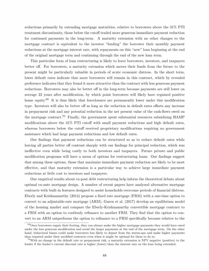
reductions primarily by extending mortgage maturities, relative to borrowers above the 31% PTItreatment discontinuity, those below the cutoff traded more generous immediate payment reductionfor continued payments in the long-term. A maturity extension with no other changes to themortgage contract is equivalent to the investor “lending” the borrower their monthly paymentreductions at the mortgage interest rate, with repayments on this “new” loan beginning at the endof the original mortgage term and continuing through the end of the new loan term.

This particular form of loan restructuring is likely to leave borrowers, investors, and taxpayersbetter off. For borrowers, a maturity extension which moves their funds from the future to thepresent might be particularly valuable in periods of acute economic distress. In the short term,lower default rates indicate that more borrowers will remain in this contract, which by revealedpreference indicates that they found it more attractive than the contract with less generous paymentreductions. Borrowers may also be better off in the long-term because payments are still lower onaverage 22 years after modification, by which point borrowers will likely have regained positivehome equity.69 It is thus likely that foreclosures are permanently lower under this modificationtype. Investors will also be better off as long as the reduction in default rates offsets any increasein prepayment risk and any potential reduction in the net present value of the cash-flows owed onthe mortgage contract.70 Finally, the government spent substantial resources subsidizing HAMPmodifications above the 31% PTI cutoff with small payment reductions and high default rates,whereas borrowers below the cutoff received proprietary modifications requiring no governmentassistance which had large payment reductions and low default rates.

Our findings that payment reductions can be structured so as to reduce default rates whileleaving all parties better off contrast sharply with our findings for principal reduction, which wasineffective even while being costly to both investors and taxpayers. Future private and publicmodification programs will have a menu of options for restructuring loans. Our findings suggestthat among these options, those that maximize immediate payment reduction are likely to be mosteffective, and that maturity extension is a particular way to achieve large immediate paymentreductions at little cost to investors and taxpayers.

Our empirical results about ex-post debt restructuring help inform the theoretical debate aboutoptimal ex-ante mortgage design. A number of recent papers have analyzed alternative mortgagecontracts with built-in features designed to assist households overcome periods of financial distress.Eberly and Krishnamurthy (2014) propose a fixed rate mortgage (FRM) with a one-time option toconvert to an adjustable-rate mortgage (ARM). Guren et al. (2017) develop an equilibrium modelof the housing market and compare the Eberly-Krishnamurthy convertible mortgage contract toa FRM with an option to costlessly refinance to another FRM. They find that the option to con-vert to an ARM outperforms the option to refinance to a FRM specifically because relative to the

69Once borrowers regain their footing, they can always make the higher mortgage payments they would have owedunder the less generous modification and avoid the larger payments at the end of the mortgage term. On the otherhand, behavioral biases could make borrowers less likely to depart from the status-quo and make higher paymentsthan required under their modified contracts even when it might be optimal for them to do so.

70With no change in the default rate or prepayment risk, a maturity extension is NPV negative (positive) to thelender if the lender’s current discount rate is higher (lower) than the interest rate on the loan being extended.

88

refinance option, the conversion to an ARM front-loads the payment reduction to the borrower,and does so at similar cost to the investor. Our results provide empirical evidence that contractsfront-loading payment reductions to households in financial distress will be more effective at pre-venting defaults than an alternative contract with equal cost to the investor that spreads paymentreductions throughout the mortgage term. Similarly, Clara and Cocco (2016) compare an ARMwith a refinance option to an ARM with the option to temporarily allow for interest-only pay-ments, with a corresponding increase in its maturity. They find that this maturity extension optionoutperforms a refinance option because it provides similar liquidity-provision benefits to borrowersat much lower cost to investors. Our results show that immediate payment reduction can indeedbe effective at reducing defaults even if structured with offsetting payments in the future so as tominimize costs to investors.

B.6 Effect of Payment Reduction on Consumption

Our payment reduction regression discontinuity empirical strategy is under-powered for studyingconsumption impacts. In Appendix Figure B.9 we plot the reduced form of the 31% PTI strategywith the change in mean credit card spending from the year before modification to the year aftermodification as the outcome variable. The standard error is so large that, using the same procedurefor calculating an MPC as described in section 4.5, we cannot rule out an MPC above 1 or below-1.

Unlike with principal reduction, we are unable to increase the precision of our payment reductionestimates by using a difference-in-differences design. The difference in principal reduction receivedby borrowers with and without principal reduction remains large when we expand the sample toa wider bandwidth. In contrast, the difference in payment reduction between HAMP and Chasemodifications falls when looking at a wider sample (as can be seen by looking at the edges ofthe top panel of Figure B.1). This is because the PTI target in HAMP generates larger paymentreduction for higher PTI borrowers. Hence comparing borrowers who received HAMP and Chasemodifications at a wider bandwidth results in a shrinking treatment size. We therefore conclude thatour data and available research designs are unsuited for credibly estimating the effect of paymentreduction on consumption.

89

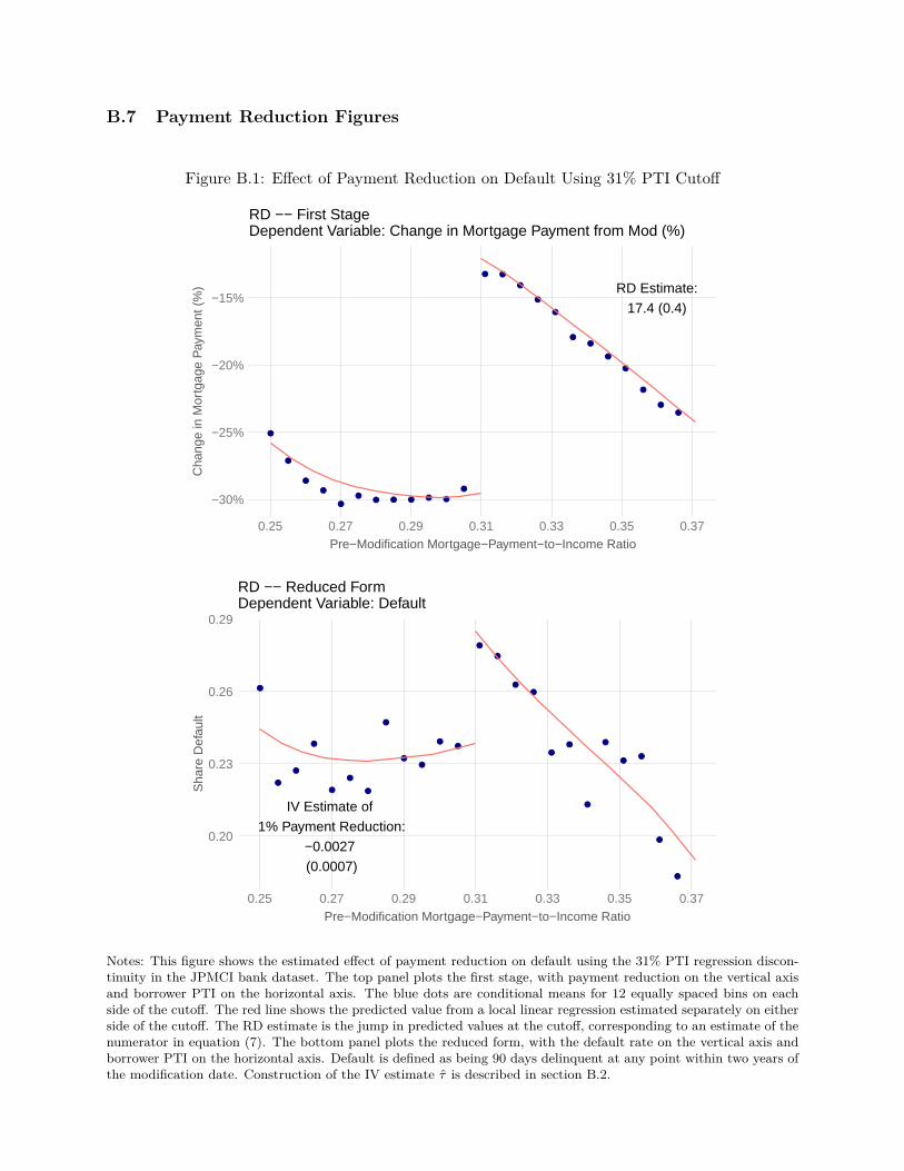
B.7 Payment Reduction Figures

Figure B.1: Effect of Payment Reduction on Default Using 31% PTI Cutoff

●

●

●

●

●

●● ● ● ● ●

●

● ●

●

●

●

●●

●

●

●

●●

RD Estimate:17.4 (0.4)

−30%

−25%

−20%

−15%

0.25 0.27 0.29 0.31 0.33 0.35 0.37Pre−Modification Mortgage−Payment−to−Income Ratio

Cha

nge

in M

ortg

age

Pay

men

t (%

)RD −− First StageDependent Variable: Change in Mortgage Payment from Mod (%)

●

●

●

●

●

●

●

●

●●

●●

●

●

●●

●●

●

●

●●

●

●

IV Estimate of 1% Payment Reduction:

−0.0027 (0.0007)

0.20

0.23

0.26

0.29

0.25 0.27 0.29 0.31 0.33 0.35 0.37Pre−Modification Mortgage−Payment−to−Income Ratio

Sha

re D

efau

lt

RD −− Reduced FormDependent Variable: Default

Notes: This figure shows the estimated effect of payment reduction on default using the 31% PTI regression discon-tinuity in the JPMCI bank dataset. The top panel plots the first stage, with payment reduction on the vertical axisand borrower PTI on the horizontal axis. The blue dots are conditional means for 12 equally spaced bins on eachside of the cutoff. The red line shows the predicted value from a local linear regression estimated separately on eitherside of the cutoff. The RD estimate is the jump in predicted values at the cutoff, corresponding to an estimate of thenumerator in equation (7). The bottom panel plots the reduced form, with the default rate on the vertical axis andborrower PTI on the horizontal axis. Default is defined as being 90 days delinquent at any point within two years ofthe modification date. Construction of the IV estimate τ̂ is described in section B.2.

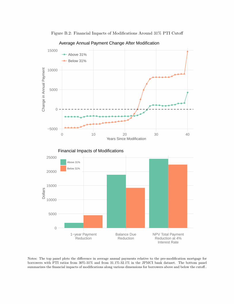
Figure B.2: Financial Impacts of Modifications Around 31% PTI Cutoff

● ● ● ● ●● ● ● ● ● ● ● ● ● ● ● ● ● ● ● ● ● ● ●

●●

●

●● ● ● ● ● ● ● ●

● ● ●

●

−5000

0

5000

10000

15000

0 10 20 30 40Years Since Modification

Cha

nge

in A

nnua

l Pay

men

t

● Above 31%

Below 31%

Average Annual Payment Change After Modification

0

5000

10000

15000

20000

25000

1−year PaymentReduction

Balance DueReduction

NPV Total PaymentReduction at 4%

Interest Rate

Dol

lars

Above 31%

Below 31%

Financial Impacts of Modifications

Notes: The top panel plots the difference in average annual payments relative to the pre-modification mortgage forborrowers with PTI ratios from 30%-31% and from 31.1%-32.1% in the JPMCI bank dataset. The bottom panelsummarizes the financial impacts of modifications along various dimensions for borrowers above and below the cutoff..

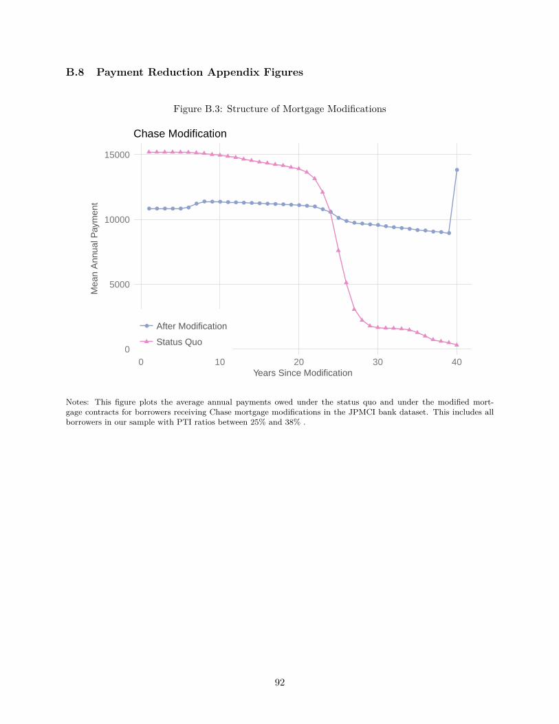
B.8 Payment Reduction Appendix Figures

Figure B.3: Structure of Mortgage Modifications

● ● ● ● ● ●● ● ● ● ● ● ● ● ● ● ● ● ● ● ● ●

●●

●● ● ● ● ● ● ● ● ● ● ● ● ● ●

●

0

5000

10000

15000

0 10 20 30 40Years Since Modification

Mea

n A

nnua

l Pay

men

t

● After Modification

Status Quo

Chase Modification

Notes: This figure plots the average annual payments owed under the status quo and under the modified mort-gage contracts for borrowers receiving Chase mortgage modifications in the JPMCI bank dataset. This includes allborrowers in our sample with PTI ratios between 25% and 38% .

92

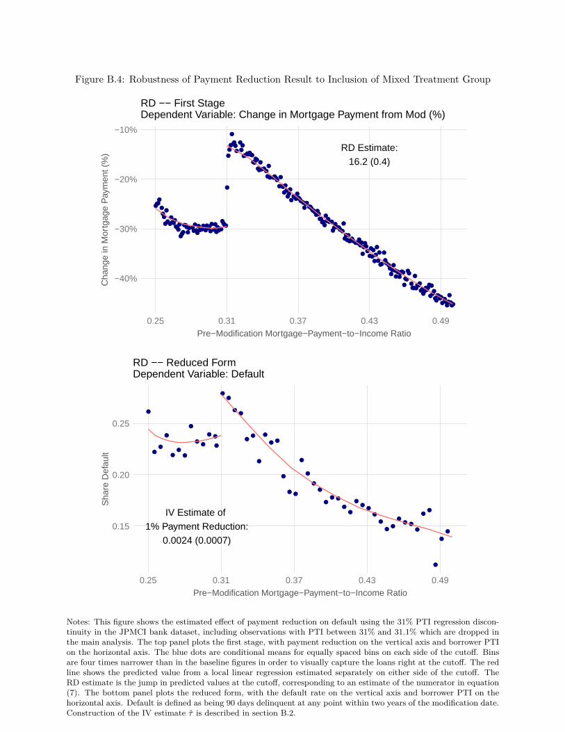
Figure B.4: Robustness of Payment Reduction Result to Inclusion of Mixed Treatment Group

●●●●

●

●●

●

●

●●

●●●●

●●●●

●●●

●●●●●●

●

●

●●

●●●

●●●●●

●

●●●

●●●●●

●●●●

●

●

●●

●

●●●●

●

●●

●●●●●●●

●●●●

●●

●

●●●●

●

●●●●●

●

●

●●●

●●

●●●

●●●●

●●●●●

●●●

●●●●●●●●●●●●●●

●●●●●

●●●●●●●

●

●●●●

●●●●●●●

●●●

●

●●●●●

●

●

●

●

●

●

●

●

●●

●

●●●

●●●●●

●●●●●●●

●

●●

●●

●●●

●

●●●●

●●●●●●●

●

●

●

●●

●●●●●●

●●●●●

●

●●●

RD Estimate:

16.2 (0.4)

−40%

−30%

−20%

−10%

0.25 0.31 0.37 0.43 0.49Pre−Modification Mortgage−Payment−to−Income Ratio

Cha

nge

in M

ortg

age

Pay

men

t (%

)RD −− First StageDependent Variable: Change in Mortgage Payment from Mod (%)

●

●●

●

●●

●

●

●●

● ●

●

●●

●●

●●

●

●

● ●

●

● ●

●

●

●

●

●● ●

●●

●●

●

●

●

●●

●● ●

●

●●

●

●

●

IV Estimate of

1% Payment Reduction:

0.0024 (0.0007)

0.15

0.20

0.25

0.25 0.31 0.37 0.43 0.49Pre−Modification Mortgage−Payment−to−Income Ratio

Sha

re D

efau

lt

RD −− Reduced FormDependent Variable: Default

Notes: This figure shows the estimated effect of payment reduction on default using the 31% PTI regression discon-tinuity in the JPMCI bank dataset, including observations with PTI between 31% and 31.1% which are dropped inthe main analysis. The top panel plots the first stage, with payment reduction on the vertical axis and borrower PTIon the horizontal axis. The blue dots are conditional means for equally spaced bins on each side of the cutoff. Binsare four times narrower than in the baseline figures in order to visually capture the loans right at the cutoff. The redline shows the predicted value from a local linear regression estimated separately on either side of the cutoff. TheRD estimate is the jump in predicted values at the cutoff, corresponding to an estimate of the numerator in equation(7). The bottom panel plots the reduced form, with the default rate on the vertical axis and borrower PTI on thehorizontal axis. Default is defined as being 90 days delinquent at any point within two years of the modification date.Construction of the IV estimate τ̂ is described in section B.2.

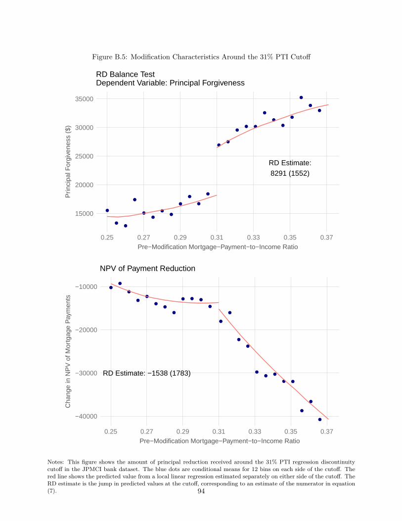
Figure B.5: Modification Characteristics Around the 31% PTI Cutoff

●

●●

●

●●

●●

●

●

●

●

●●

●● ●

●

●

●

●

●

●

●

RD Estimate:

8291 (1552)

15000

20000

25000

30000

35000

0.25 0.27 0.29 0.31 0.33 0.35 0.37Pre−Modification Mortgage−Payment−to−Income Ratio

Prin

cipa

l For

give

ness

($)

RD Balance TestDependent Variable: Principal Forgiveness

●●

●

●●

●●

●

● ● ●

●

●

●

●

●

●● ●

● ●

●

●

●

RD Estimate: −1538 (1783)

−40000

−30000

−20000

−10000

0.25 0.27 0.29 0.31 0.33 0.35 0.37Pre−Modification Mortgage−Payment−to−Income Ratio

Cha

nge

in N

PV

of M

ortg

age

Pay

men

ts

NPV of Payment Reduction

Notes: This figure shows the amount of principal reduction received around the 31% PTI regression discontinuitycutoff in the JPMCI bank dataset. The blue dots are conditional means for 12 bins on each side of the cutoff. Thered line shows the predicted value from a local linear regression estimated separately on either side of the cutoff. TheRD estimate is the jump in predicted values at the cutoff, corresponding to an estimate of the numerator in equation(7). 94

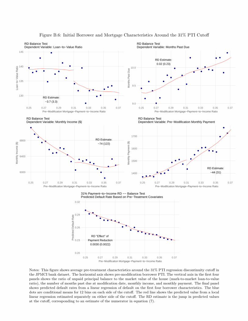
Figure B.6: Initial Borrower and Mortgage Characteristics Around the 31% PTI Cutoff

●

●●

●

●

●

●

●

●

●

●

●

●

●

●

●

●●

●●

●

●●

●RD Estimate:

−3.7 (3.3)

130

135

140

145

0.25 0.27 0.29 0.31 0.33 0.35 0.37Pre−Modification Mortgage−Payment−to−Income Ratio

Loan

−to

−V

alue

Rat

io

RD Balance TestDependent Variable: Loan−to−Value Ratio

●

●

●

●

●

●

●

●

●

●

●

●

●

●

●

●

●

●

● ●

● ●

●

●

RD Estimate:0.02 (0.23)

9.0

9.5

10.0

0.25 0.27 0.29 0.31 0.33 0.35 0.37Pre−Modification Mortgage−Payment−to−Income Ratio

Mon

ths

Pas

t Due

RD Balance TestDependent Variable: Months Past Due

●

●

●

●●

●

● ●

●●

●

●

●

●●

●

●●

●

●

●

●

●

●

RD Estimate:−74 (122)

6000

6400

6800

0.25 0.27 0.29 0.31 0.33 0.35 0.37Pre−Modification Mortgage−Payment−to−Income Ratio

Mon

thly

Inco

me

($)

RD Balance TestDependent Variable: Monthly Income ($)

●● ●

●

●● ●

●

●

●●

●

●

●

●

●

● ●

● ●●

●

●

●

RD Estimate:−44 (31)1400

1500

1600

1700

0.25 0.27 0.29 0.31 0.33 0.35 0.37Pre−Modification Mortgage−Payment−to−Income Ratio

Mon

thly

Pay

men

t ($)

RD Balance TestDependent Variable: Pre−Modification Monthly Payment

●

●●

●

●

● ● ●●

●

●●

●

●

●●

● ● ● ●

●●

● ●

RD "Effect" of Payment Reduction

0.0030 (0.0022)

0.20

0.23

0.26

0.29

0.32

0.25 0.27 0.29 0.31 0.33 0.35 0.37Pre−Modification Mortgage−Payment−to−Income Ratio

Pre

dict

ed D

efau

lt R

ate

31% Payment−to−Income RD −− Balance TestPredicted Default Rate Based on Pre−Treatment Covariates

Notes: This figure shows average pre-treatment characteristics around the 31% PTI regression discontinuity cutoff inthe JPMCI bank dataset. The horizontal axis shows pre-modification borrower PTI. The vertical axis in the first fourpanels shows the ratio of unpaid principal balance to the market value of the house (mark-to-market loan-to-valueratio), the number of months past due at modification date, monthly income, and monthly payment. The final panelshows predicted default rates from a linear regression of default on the first four borrower characteristics. The bluedots are conditional means for 12 bins on each side of the cutoff. The red line shows the predicted value from a locallinear regression estimated separately on either side of the cutoff. The RD estimate is the jump in predicted valuesat the cutoff, corresponding to an estimate of the numerator in equation (7).

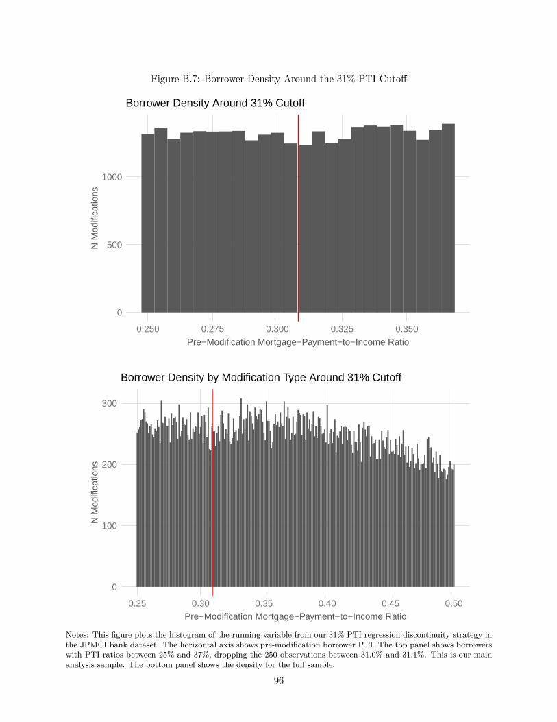
Figure B.7: Borrower Density Around the 31% PTI Cutoff

0

500

1000

0.250 0.275 0.300 0.325 0.350Pre−Modification Mortgage−Payment−to−Income Ratio

N M

odifi

catio

nsBorrower Density Around 31% Cutoff

0

100

200

300

0.25 0.30 0.35 0.40 0.45 0.50Pre−Modification Mortgage−Payment−to−Income Ratio

N M

odifi

catio

ns

Borrower Density by Modification Type Around 31% Cutoff

Notes: This figure plots the histogram of the running variable from our 31% PTI regression discontinuity strategy inthe JPMCI bank dataset. The horizontal axis shows pre-modification borrower PTI. The top panel shows borrowerswith PTI ratios between 25% and 37%, dropping the 250 observations between 31.0% and 31.1%. This is our mainanalysis sample. The bottom panel shows the density for the full sample.

96

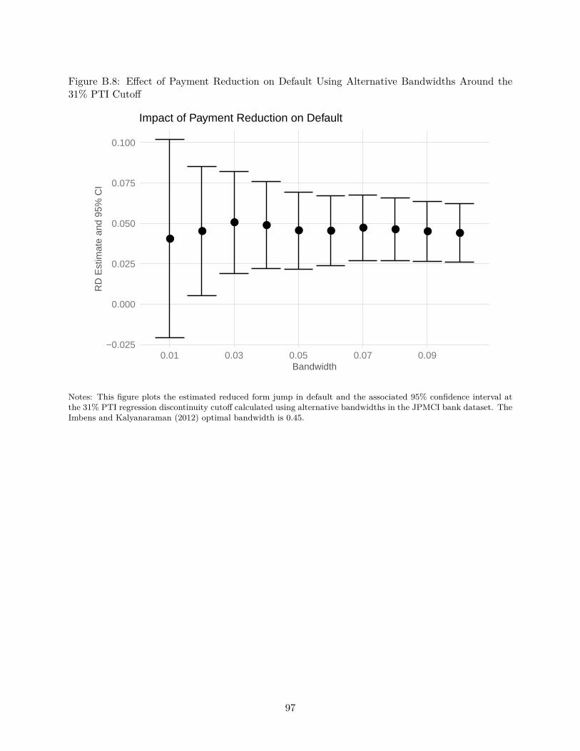
Figure B.8: Effect of Payment Reduction on Default Using Alternative Bandwidths Around the31% PTI Cutoff

●●

● ●● ● ● ● ● ●

−0.025

0.000

0.025

0.050

0.075

0.100

0.01 0.03 0.05 0.07 0.09Bandwidth

RD

Est

imat

e an

d 95

% C

I

Impact of Payment Reduction on Default

Notes: This figure plots the estimated reduced form jump in default and the associated 95% confidence interval atthe 31% PTI regression discontinuity cutoff calculated using alternative bandwidths in the JPMCI bank dataset. TheImbens and Kalyanaraman (2012) optimal bandwidth is 0.45.

97

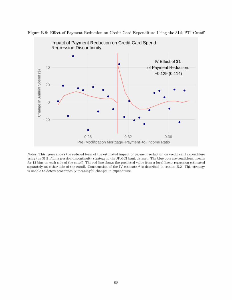
Figure B.9: Effect of Payment Reduction on Credit Card Expenditure Using the 31% PTI Cutoff

●

●

●

●

●●

●

●

●

●

●

●

●

●

●

●

●

●

●

●●

●

●

●

●

●

IV Effect of $1

of Payment Reduction:

−0.129 (0.114)

−20

0

20

40

0.28 0.32 0.36Pre−Modification Mortgage−Payment−to−Income Ratio

Cha

nge

in A

nnua

l Spe

nd (

$)Impact of Payment Reduction on Credit Card Spend Regression Discontinuity

Notes: This figure shows the reduced form of the estimated impact of payment reduction on credit card expenditureusing the 31% PTI regression discontinuity strategy in the JPMCI bank dataset. The blue dots are conditional meansfor 12 bins on each side of the cutoff. The red line shows the predicted value from a local linear regression estimatedseparately on either side of the cutoff. Construction of the IV estimate τ̂ is described in section B.2. This strategyis unable to detect economically meaningful changes in expenditure.

98