The XFEM for high-gradient solutions in convection … Webseite...XFEM FOR CONVECTION-DOMINATED HIGH GRADIENT SOLUTIONS 1 In this paper, we focus on advection-dominated problems as

Aachen Institute for Advanced Study in Computational Engineering Science

Preprint: AICES-2009-15

03/August/2009

The XFEM for high-gradient solutions in

convection-dominated problems

Safdar Abbas, Alaskar Alizada and Thomas-Peter Fries

Financial support from the Deutsche Forschungsgemeinschaft (German Research Association) through

grant GSC 111 is gratefully acknowledged.

©Safdar Abbas, Alaskar Alizada and Thomas-Peter Fries 2009. All rights reserved

List of AICES technical reports: http://www.aices.rwth-aachen.de/preprints

http://www.aices.rwth-aachen.de/preprints

The XFEM for high-gradient solutionsin convection-dominated problems

Safdar Abbas1 Alaskar Alizada2 and Thomas-Peter Fries2 !

1 AICES, RWTH Aachen University, Schinkelstr. 2, 52062 Aachen, Germany2 CATS, RWTH Aachen University, Schinkelstr. 2, 52062 Aachen, Germany

SUMMARY

Convection-dominated problems typically involve solutions with high gradients near the domainboundaries (boundary layers) or inside the domain (shocks). The approximation of such solutionsby means of the standard finite element method requires stabilization in order to avoid spuriousoscillations. However, accurate results may still require a mesh refinement near the high gradients.Herein, we investigate the extended finite element method (XFEM) with a new enrichment schemethat enables highly accurate results without stabilization or mesh refinement. A set of regularizedHeaviside functions is used for the enrichment in the vicinity of the high gradients. Di!erent linearand non-linear problems in one and two dimensions are considered and show the ability of the proposedenrichment to capture arbitrary high gradients in the solutions. Copyright c! 2009 John Wiley &Sons, Ltd.

key words: Extended finite element method (XFEM), high-gradient solutions, convection-di!usion,

convection-dominated, boundary layers, shocks.

1. Introduction

The finite element method (FEM) has been extensively used to approximate the solution ofpartial di!erential equations. The technique has been perfected in many ways for smoothsolutions, however, its application to discontinuous or singular solutions is not trivial. Inorder to approximate discontinuous solutions, the element edges need to be aligned to thediscontinuity. For singularities and high gradients, mesh refinement is needed. Moreover,for a moving discontinuity, re-meshing the computational domain imposes an additionalcomputational e!ort. The extended finite element method (XFEM) [1, 2] has the potentialto overcome these problems and produces accurate results without aligning elements todiscontinuities and without refining the mesh near singularities. These properties have madethe XFEM a particularly good choice for the simulation of cracks, see e.g. [3, 4, 5, 6], as in thisapplication, both, discontinuities (across the crack surface) and high gradients (at the crackfront) are present.

!Correspondence to: [email protected]

XFEM FOR CONVECTION-DOMINATED HIGH GRADIENT SOLUTIONS 1

In this paper, we focus on advection-dominated problems as they naturally occur in fluiddynamics and many other transport problems. For such problems, high gradients are observednear the domain boundaries (boundary layers) or inside the domain (shocks). Stabilizationis typically needed in the context of the standard FEM [7, 8, 9] in order to avoid spuriousoscillations. However, even with stabilization, high gradients are often still not representedsu"ciently accurate on coarse meshes and mesh refinement is still needed in addition. Thisapplies for Continuous Galerkin methods [7, 10, 8] as well as for the Discontinuous Galerkinmethods [11, 12].

We employ the XFEM with the aim to approximate convection-dominated problems withoutstabilization or mesh refinement. A new enrichment scheme is proposed that enables theapproximation to capture arbitrary high gradients. We want to avoid an adaptive procedurewhich determines one suitable enrichment function through an iterative procedure which thenneeds to be realized within each time-step. In contrast, we rather provide a set of enrichmentfunctions near the largest gradient (i.e. along the boundary or near a shock). This set is basedon regularized Heaviside functions and is able to treat all gradients starting from the gradientthat can no longer be represented well by the standard FEM approximation up to the case ofalmost a jump. It is noted that in the presence of di!usion, no matter how small, true jumpsin the solutions are impossible and the use of the step enrichment, being standard in manyapplications of the XFEM, is not allowed (due to continuity considerations from functionalanalysis).

The use of regularized step functions in the XFEM has been realized in the simulationof cohesive cracks and shear bands: Patzak and Jirasek [13] employed regularized Heavisidefunctions for resolving highly localized strains in narrow damage process zones of quasibrittlematerials. Thereby, they incorporate the non-smooth behavior in the approximation space.Arieas and Belytschko [14] embedded a fine scale displacement field with a high strain gradientaround a shear band. They used a tangent hyperbolic type function for the enrichment.Benvenuti [15] also used a similar function for simulating the embedded cohesive interfaces.Waisman and Belytschko [16] proposed a parametric adaptive strategy for capturing highgradient solutions. One enrichment function is designed to match the qualitative behavior ofthe exact solution with a free parameter. The free parameter is optimized by using a-posteriorierror estimates.

In [13, 14, 15], the regularized Heaviside functions depend on physical considerations. Onlyone enrichment function is used in [14, 16]. A common feature of most previous applicationsis that the change from 0 to 1 takes place within one element. Herein, however, we show thatfor arbitrary high gradients in convection-dominated problems, the length scale where thechange from 0 to 1 takes place should exceed the element size and, consequently, extends toseveral elements around the largest gradient. Furthermore, it is found that only one enrichmentfunction cannot cover the complete range of gradients and that a set of enrichment functions isneeded. The fact that several enrichment functions are present and some of them extend overseveral elements complicates the implementation of the XFEM compared to standard XFEMapplications.

The paper is organized as follows: The general form of XFEM-approximations for multipleenrichment terms is given in Section 2. The governing equations for the considered linearand non-linear convection-dominated problems are described in Section 3. In Section 4, theenrichment scheme for the XFEM is proposed for high gradients inside the domain. Theprocedure for finding suitable sets of enrichment functions is discussed and additional issues

Copyright c" 2009 John Wiley & Sons, Ltd. Int. J. Numer. Meth. Engng 2009; 1:0–10Prepared using nmeauth.cls

2 S. ABBAS ET AL.

such as the quadrature and the removal of almost linearly dependent degrees of freedomare mentioned. Several numerical results are presented which obtain highly accurate resultswithout stabilization and mesh refinement. Section 5 gives the enrichment functions that areuseful in order to capture high gradients near the boundaries. Again, numerical results showthe success of the enrichment scheme. The paper concludes with a summary and outlook inSection 6.

2. XFEM formulation

A standard XFEM approximation of a scalar function uh(x) in a d-dimensional domain # ! Rd

is given asuh(x, t) =

!

i!I

Ni(x)ui

" #$ %strd. FE part

+!

i!I!

N!i (x) · !(x, t) ai

" #$ %enrichment

, (2.1)

for the case of only one enrichment term. Ni(x) is the standard FE function for node i, ui

is the unknown of the standard FE part at node i, I is the set of all nodes in the domain,N!

i (x) is a partition of unity function of node i, !(x, t) is the global enrichment function,ai is the unknown of the enrichment at node i, and I! is a nodal subset of enriched nodes.The functions N!

i (x) equal Ni(x) in this work although this is not necessarily the case. Theglobal enrichment function !(x, t) incorporates the known solution characteristics into theapproximation space and is time-dependent in this work. The XFEM is generally used toapproximate discontinuous solutions (strong discontinuities) or solutions having discontinuousderivatives (weak discontinuities). Then, a typical choice for the enrichment functions is: Thestep-enrichment

!(x, t) = sign("(x, t)) =

&'(

')

"1 : "(x, t) < 0,

0 : "(x, t) = 0,

1 : "(x, t) > 0,

(2.2)

for strong discontinuities (jumps) and the abs-enrichment

!(x, t) = abs("(x, t)) = |"(x, t)|, (2.3)

for weak discontinuities (kinks).It is noted that these enrichment functions depend on the level-set function "(x, t) which is

typically the signed-distance function. Assuming that "d(x, t) is the shortest distance at timet of every point x in the domain to the (moving) discontinuity, then

"(x, t) =

*""d(x, t) #x ! #",

+"d(x, t) #x ! #+,(2.4)

where #" and #+ are the two subdomains on the opposite sides of the interface. See [17, 18]for further details on the level-set method.

Let us now adapt the XFEM approximation and level-set concept for the situation relevantfor convection-dominated problems. The level-set function is used to describe the position ofthe largest gradient, i.e. the position of the shock, inside the domain. It is assumed that this



position is known in the initial situation (at time t = 0). However, the development of theposition of the largest gradient (the shock) in time is typically not known and not needed forthe proposed technique. Instead, an additional transport equation for the level-set functionis solved which appropriately accounts for the movement in time; this shall be seen in moredetail later. For large gradients near the boundary, i.e. for boundary layers, the position of thelargest gradient is directly the boundary itself, so that the level-set concept is not needed then.The enrichment functions for boundary layers depend only on the discretization near the wall.

As mentioned above, several enrichment functions are needed in order to capture arbitraryhigh gradients in convection-dominated problems. Therefore, the XFEM-approximation (2.1)is extended in a straightforward manner as

uh(x, t) =!

i!I

Ni(x)ui +m!

j=1

!

i!I!j

N!i (x) · !j(x, t) aj

i , (2.5)

where m is the number of enrichment terms. It is noted that each enrichment function !j(x, t)may refer to a di!erent set of enriched nodes I!

j .

3. Governing equations

In this work, numerical results will be presented individually in Sections 4 and 5 for solutionswith high gradients inside the domain and at the boundary, respectively. Therefore, itproves useful to define the governing equations of the considered advection-di!usion problemsbeforehand. Linear and non-linear advection-di!usion problems are considered in one and twodimensions.

3.1. Linear advection-di!usion equation

Let # be an open, bounded region in # ! Rd. The boundary is denoted by $ and is assumedsmooth. The linear advection-di!usion problem with prescribed constant velocities c ! Rd anda constant, scalar di!usion parameter # ! R is stated in the following initial/boundary valueproblem: Find u(x, t) #x ! # and #t ! [0, T ] such that

u(x, t) = "c ·$u + # ·%u, in # % ]0, T [, (3.1)u(x, 0) = u0(x), #x ! # (3.2)u(x, t) = u(x, t), #x ! $ % ]0, T [, (3.3)

where %u = $ · ($u) and u = $u/$t. The initial condition u0 : # & R and Dirichletboundary condition u : $%]0, T [& R are prescribed data. No Neumann boundary conditionsare considered.

For the approximation with finite elements, the problem has to be stated in its discretizedvariational form. The variational form also depends on the time-discretization: If the derivativein time is treated by finite di!erences the test and trial function spaces are

ShTS =

+uh ! H1h(#) | uh = uh on $

,, (3.4)

VhTS =

+wh ! H1h(#) | wh = 0 on $

,, (3.5)


4 S. ABBAS ET AL.

where “TS” stands for “time stepping”. H1h is a finite dimensional subspace of the spaceof square-integrable functions with square-integrable first derivatives H1. H1h is spanned bythe standard finite element and enrichment functions given in the approximation (2.5). Theobjective is to find uh ! Sh

TS, such that #wh ! VhTS:

-

!wh

.uh + c ·$uh

/d#+ #

-

!$wh ·$uhd# =0 . (3.6)

Time!slab

Position of thehighest gradient

t"n

t

x

tn+1

t+n

Figure 1. Space-time discretization for the discontinuous Galerkin method in time.

In this work, we also consider the discontinuous Galerkin method in time for the time-discretization, see e.g. [9]. The space-time domain Q = #%]0, T [ is divided into time slabsQn = #%]tn, tn+1[, where 0 = t0 < t1 < . . . < tN = T . Each time slab is discretized byextended space-time finite elements, see Figure 1. The enriched approximation is of the form(2.5), however, the finite element shape functions are now also time-dependent, i.e. Ni(x, t)and N!

i (x, t). The test and trial function spaces are

ShST =

+uh ! H1h(Qn) | uh = uh on $%]tn, tn+1[

,, (3.7)

VhST =

+wh ! H1h(Qn) | wh = 0 on $%]tn, tn+1[

,, (3.8)

and are again spanned by the FE shape functions and enrichment functions in (2.5). “ST”stands for “space-time”. The discretized weak form may be formulated as follows: Given

.uh

/"n

,find uh ! Sh

ST such that #wh ! VhST

-

Qn

wh.uh + c ·$uh

/dQ + #

-

Qn

$wh ·$uhdQ, (3.9)

+-

!n

.wh

/+

n·0.

uh/+

n"

.uh

/"n

1d# =0 , (3.10)

where.uh

/±n

is.uh

/±n

= lim"#0

uh (x, tn ± %) . (3.11)

The continuity of the field variables is weakly enforced across the time-slabs, see (3.10). Theinitial condition uh

0 is set for.uh

/"0

.



It is noted that Equation (3.6) on the one hand and Equations (3.9) and (3.10) on the otherhand are both Bubnov-Galerkin weighted residual formulations. That is, no stabilization termsare present. The results obtained by the unstabilized XFEM approximations are comparedlateron with both stabilized and unstabilized standard FEM approximations. Stabilized weakforms in the context of the standard FEM are e.g. found in [7, 8, 19].

Remark. In order to consider for moving interfaces in the domain, a pure advection equationhas to be solved in # for the level-set function "(x, t) [17, 18]. The strong form equals Equation(3.1) to (3.3) with # = 0 and boundary conditions are only applied at the inflow.

3.2. Burgers equation

The Burgers equation in one dimension with a constant, scalar di!usion parameter # ! R isstated in the following initial/boundary value problem: Find u(x, t) #x ! # and #t ! [0, T ]such that

u(x, t) = "u · $u

$x+ # · $2u

$x2, in # % ]0, T [, (3.12)

u(x, 0) = u0(x), #x ! # (3.13)u(x, t) = u(x, t), #x ! $ % ]0, T [. (3.14)

The initial condition u0 and Dirichlet boundary condition u are prescribed data. No Neumannboundary conditions are considered.

The variational form for a finite di!erence treatment of the temporal derivative is to finduh ! Sh

TS, such that #wh ! VhTS:

-

!wh

2uh + uh · $uh

$x

3d#+ #

-

!

$wh

$x· $uh

$xd# = 0, (3.15)

and for the discontinuous Galerkin method in time: Given.uh

/"n

, find uh ! ShST such that

#wh ! VhST

-

Qn

wh

2uh + uh · $uh

$x

3dQ + #

-

Qn

$wh

$x· $uh

$xdQ, (3.16)

+-

!n

.wh

/+

n·0.

uh/+

n"

.uh

/"n

1d# =0 . (3.17)

4. XFEM for high gradients inside the domain (shocks)

In the following, an overview over existing regularized step functions is given. A particularsuitable choice for high gradients inside the domain is discussed. The next step is to define aset of these functions in order to capture arbitrary gradients. An optimization procedure isdescribed which is used to determine sets of 3, 5, and 7 enrichment functions.

4.1. Di!erent classes of regularized step functions

In this work, a minimum requirement of a regularized step function that can be used as anenrichment function for high gradients in the domain is that they depend on the level-set


6 S. ABBAS ET AL.

function "(x, t). The zero-level of "(x, t) is the centerline of the highest gradient (shock).Furthermore, we need control over the gradient of the regularized step function. This can be aparameter that directly scales the gradient, see Figure 2(a), or which controls the gradientindirectly by prescribing the length-scale where the change from 0 to 1 takes place, seeFigure 2(b). In addition the function is constant for |"| > &.

1

m

x

!

(a)

!

x"" +"

(b)

Figure 2. Regularized Heaviside function for a high gradient enrichment: (a) the gradient is scaleddirectly, (b) the gradient is scaled indirectly by controlling the width.

Three di!erent choices of enrichment functions are investigated. The first function is adaptedfrom Areias and Belytschko [14] and depends on a parameter & that specifies the width ofthe function and a parameter n that specifies the gradient of the function. By “width” ofthe regularized step function, we refer to the region where the function varies monotonicallybetween 0 (or "1) and 1. The higher the value of n, the steeper will be the function for thesame width &.

!("(x, t), &, n) =

&''(

'')

"1, if "(x, t) < "&,tanh(n"(x, t))

tanh(n&), if |"(x, t)| ! &,

1, if "(x, t) > &.

(4.1)

This function is C$-continuous in the domain except at $# = {x ! # : |"(x, t)| = &} where itis C0-continuous only, i.e. there is a kink at $#. This may complicate the numerical integrationand artificial weak discontinuities are introduced. Consequently, for the applications consideredherein it is desirable to have functions that are more than C0-continuous in the overall domain.

The second function is the following regularization function taken from Benvenuti [15]. Thisfunction depends on only one parameter n which scales the gradient. The smaller the value ofn, the larger is the gradient of the function

!(", &) = sign(")01 " exp(

"|"|n

)1. (4.2)

The problem with function (4.2) is that it does not allow for a direct control of the width.The third function is a piecewise polynomial function taken from Patzak and Jirasek [13].

This function only depends on one parameter & that controls the width of the function directly.



Thereby, also the gradient is a!ected so that smaller & lead to larger gradients. The functionis

!(", &) =

&'''(

''')

0, if " < "&,

1V#

- $

"#

01 " '2

&2

14d', if |"| ! &,

1, if " > &,

(4.3)

where the reference volume V# determines the continuity properties of the function at $#.The function is C2-continuous for V# = 16&/15 and C4-continuous for V# = 256&/315. UsingV# = 256&/315 and evaluating the integral involved in (4.3) gives

!(", &) =1

256&9

2128&9 + 315"&8 " 420"3&6 + 378"5&4 " 180"7&2 + 35"9

3(4.4)

for |"(x, t)| ! &. Definition (4.3) is C$-continuous in the domain, except at $# where it isC4-continuous (compared to C0-continuity of function (4.1)) and it allows a direct control ofthe width. Therefore, we prefer (4.3) over (4.1) and (4.2) and use it throughout the remainingof this work. For other examples of regularized heaviside functions, see [20].

−1 −0.8 −0.6 −0.4 −0.2 0 0.2 0.4 0.6 0.8 1

−1

−0.8

−0.6

−0.4

−0.2

0

0.2

0.4

0.6

0.8

1

−! !

"

#

Enr. Func.(23), ! = 0.1, n = 20Enr. Func.(24), ! = 0.1

(a)

−1 −0.8 −0.6 −0.4 −0.2 0 0.2 0.4 0.6 0.8 1

0

0.2

0.4

0.6

0.8

1

−! !

"

#

Enr. Func.(25), ! = 0.1

(b)

Figure 3. Comparative plot of regularized Heaviside functions for ! = 0.1: (a) for (4.1) and (4.2), (b)for (4.3).

It is important to note that the width & should depend on the element size h of the mesh. Aconstant width could lead to situations where & ' h, and the resulting enrichment functionswould not span a good basis (i.e. the condition number would increase prohibitively). Thefact that the width depends on the discretization rather than on physical considerations is incontrast to previous applications of regularized step functions in the frame of cohesive cracksand shear bands.

4.2. Optimal set of enrichment functions

The aim is to cover the complete range of high gradients starting from the gradient that canbe no longer represented well by the standard FEM approximation up to the case of almost a


8 S. ABBAS ET AL.

(a) 3 enrichment functions

Enr. Func. &/h!1 2.5!2 0.27!3 0.0225

(b) 5 enrichment functions

Enr. Func. &/h!1 2.5!2 0.85!3 0.265!4 0.085!5 0.0225

(c) 7 enrichment functions

Enr. Func. &/h!1 2.5!2 1.5!3 0.5!4 0.25!5 0.125!6 0.0625!7 0.0225

Table I. Optimal sets of enrichment functions, h is a characteristic element size near the shock.

jump (the gradient is then extremely large). For that purpose, one enrichment function is notsu"cient. In contrast, several enrichment functions have to be chosen.

For a given number m of enrichment functions ! = {!1(", &1), . . . ,!m(", &m)}, anoptimization procedure is employed in order to determine the corresponding values &1, . . . , &m.The aim is to minimize the largest pointwise error

%(!) = sup(uh(x) " f(x)) #x ! # (4.5)

of the following interpolation problem-

!wh uh(x) =

-

!wh f(x) in # (4.6)

where f(x) is a given regularized step function that shall be interpolated by the m (enrichment)functions of (4.3), i.e.

uh(x) =m!

j=1

!j(", &j). (4.7)

The domain is # =]0, 1[ and " = x " 0.5 is a time-independent level-set function, whose zero-level is at x = 0.5, i.e. where the gradient of f(x) is maximum. An important point is that foreach prescribed set of enrichment functions ! (which here are regular interpolation functionsbased on (4.3)), the gradient of the function f(x) is varied systematically between a minimumand a maximum gradient. For each set !, the largest value for % is stored in %total. The optimalset for each number m is then the one with the smallest %total. In this way, optimal sets arefound for three, five and seven enrichment functions. A graphical representation of these setsis given in Figures 4(a)-4(c).

The next step is to use this set of functions within an XFEM approximation of the form(2.5). The functions have to be scaled with respect to the element size. Therefore, the resultingwidths &1, · · · &m in table I depend on h. It is seen that some of these functions vary between0 and 1 over more than one element. For a given enrichment function !j , it is important toenrich the nodes (through the choice of I!

j ) of all elements where !j varies between 0 and 1.The appropriate nodes are easily determined by means of the value of the level-set functionat each node which is directly the distance to the shock. It is noted that in standard XFEMapplications, where the step- and abs-enrichment of Equations (2.2) and (2.3) is used, only thenodes of elements that are crossed by the zero-level of " are enriched, i.e. in I!.



In the following, all results are obtained for the set of seven enrichment functions. It isimportant to recall that these widths are relative to the element sizes near the shock. That is,the widths decrease with mesh refinement and vice versa.

4.3. Quadrature

In the case of XFEM approximations with discontinuous enrichments, elements are subdividedinto sub-cells for integration purposes [2]. For continuous enrichment functions as used in thiswork, this subdivision is not necessarily required. However, due to the high gradients of theenrichment functions inside the element, a large number of integration points may be neededfor accurate quadrature.

It is well-known that Gauss quadrature rules concentrate integration points near the elementedges, see Figure 5(a) for the example of three quadrilateral elements. It is desirable toconcentrate integration points near the shock where the enrichment functions have highgradients, too. Therefore, we found that a subdivision as known from most XFEM applicationswith discontinuous enrichments is also advantageous for the high gradient enrichmentsproposed herein. This is confirmed in a number of studies and it is found that, for a givenlevel of accuracy of the quadrature, less integration points are needed for the decompositioninto integration subcells than without. An example of the resulting integration points is givenin Figure 5(b) where the thick dashed line shows the position of the highest gradient inthe two-dimensional domain or the zero level of the level-set function and the thin dasheddiagonals represent the quadrature subcells for integration. It can be seen that the density ofthe integration points is large near the shock as desired. More advanced quadrature schemesfor high gradient integrands are discussed e.g. in [20, 14, 21] and are not in the focus of thiswork.

4.4. Blocking of some enriched degrees of freedom

In the case of discontinuous functions, only the nodes of cut elements are enriched with a stepfunction. It is then well-known that if the di!erence of the element areas/volumes on the twosides of the interface is increasingly large, then the enrichment becomes more and more linearlydependent [22, 23]. It is then useful to remove those degrees of freedom whose contribution tothe overall system of equations is negligible. This can be called “blocking” degrees of freedom.

The situation is similar for the proposed enrichment scheme for high gradient solutions insidethe domain. We found that a simple procedure for the blocking can be used for the test casesconsidered in this work: Once the final system matrix is assembled, the absolute maximumvalue of each row of the enriched degrees of freedom is determined. If this value is less thana specific tolerance, e.g. 10"7, the corresponding degree of freedom is blocked. In this way,without a!ecting the accuracy of the approximation noticeably, the conditioning of the systemremains within a reasonable threshold.

4.5. Numerical examples with high gradients inside the domain

Four in-stationary convection-dominated problems are considered in order to show thee!ectiveness of the enrichment scheme. The optimal set of seven enrichment functions describedin Section 4.2 is used to enrich the approximation space. The position of the highest gradientis represented by the zero-level of a level-set function.


10 S. ABBAS ET AL.

0 0.1 0.2 0.3 0.4 0.5 0.6 0.7 0.8 0.9 10

0.1

0.2

0.3

0.4

0.5

0.6

0.7

0.8

0.9

1

0.2 0.25 0.3 0.35 0.4 0.45 0.5

0

0.01

0.02

0.03

0.04

0.05

0.06

(a) Optimal set of three enrichment functions

0 0.1 0.2 0.3 0.4 0.5 0.6 0.7 0.8 0.9 10

0.1

0.2

0.3

0.4

0.5

0.6

0.7

0.8

0.9

1

0.2 0.25 0.3 0.35 0.4 0.45 0.50

0.01

0.02

0.03

0.04

0.05

(b) Optimal set of five enrichment functions

0 0.1 0.2 0.3 0.4 0.5 0.6 0.7 0.8 0.9 10

0.1

0.2

0.3

0.4

0.5

0.6

0.7

0.8

0.9

1

0.2 0.25 0.3 0.35 0.4 0.45 0.5

0

0.005

0.01

0.015

0.02

0.025

0.03

0.035

0.04

0.045

(c) Optimal set of seven enrichment functions

Figure 4. Optimal sets of enrichment functions. The boxes in the left figures show the regions whichare zoomed out in the right figures.



(a)

(b)

Figure 5. Integration points in quadrilateral elements, (a) without partitioning, (b) with partitioningwith respect to the position of the highest gradient.

4.5.1. Burgers equation with stationary high gradient developing over time The Burgersequation in one dimension is considered first, see Section 3.2 for the governing equations.The domain is # =]0, 1[ and T = 1. The initial condition is given as u0(x) = sin 2((x). Inthis setting, the gradient at x = 0.5 increases over time withough changing the position of thehighest gradient in #. The maximum gradient over time depends on the di!usion coe"cient #,and, as long as # > 0, the gradient is finite. However, for small di!usion coe"cients very highgradients develop at x = 0.5. Herein, # is chosen as 1.25 % 10"3. The temporal discretizationis achieved through the Crank-Nicolson method where u = F (u, t) is replaced by

un+1 " un

(t=

12.F (un+1, tn+1) + F (un, tn)

/. (4.8)

Consequently, the variational form (3.15) applies. The nonlinear term u · u,x is linearized bythe Newton-Raphson method.

Linear finite element shape functions are used for Ni(x) and N!i (x) in the XFEM

approximation (2.5). The mesh consists of an even number of equally-spaced nodes. Thus,the highest gradient at x = 0.5 is always present in the middle of the center element. Theinitial position of the highest gradient is known and does not change during the computation.Therefore, the level-set function, "(x) = x " 0.5, does not change in time and all enrichmentfunctions are time-independent. Then, time-stepping methods such as the Crank-Nicolsonmethod can be used in the standard way. It is noted that for moving high gradients, theenrichment functions are time-dependent which e!ects the time discretization. Time-steppingschemes are then to be used with care as discussed in [24, 25]. Consequently, for all subsequent


12 S. ABBAS ET AL.

test-cases with moving high gradients we employ the discontinuous Galerkin method in time(i.e. space-time elements).

0 0.1 0.2 0.3 0.4 0.5 0.6 0.7 0.8 0.9 1−4

−3

−2

−1

0

1

2

3

4

(a) Unstabilized FEM results.

0 0.1 0.2 0.3 0.4 0.5 0.6 0.7 0.8 0.9 1−2.5

−2

−1.5

−1

−0.5

0

0.5

1

1.5

2

2.5

(b) FEM results with SUPG stabilization.

0 0.1 0.2 0.3 0.4 0.5 0.6 0.7 0.8 0.9 1−2

−1.5

−1

−0.5

0

0.5

1

1.5

2

(c) Unstabilized XFEM results.

Figure 6. Results for the 1D Burgers Equation.

Figure 6(a) shows the results obtained by the standard FEM without using stabilizationor refinement, based on a mesh with 21 linear elements (22 degrees of freedom) and 20 time-steps. Solutions at some intermediate time steps are shown and the exact solution at the finaltime T is shown by a thick, gray line. Large oscillations are observed in the FEM solutionas expected. When solving the SUPG-stabilized weak form of this problem, see e.g. [7], theoscillations are considerably reduced but the accuracy is still low, see Figure 6(b). The XFEMresults on the same mesh without stabilization are shown in Figure 6(c). The approximationspace is enriched by the set of seven enrichment functions resulting in 42 degrees of freedomof the overall enriched approximation. No oscillations are visible in the XFEM solution.

Figure 7 compares the XFEM and FEM solutions in terms of the error in the L2-Norm



102 103 104

10−4

10−3

10−2

10−1

100

2

1

Degrees of Freedom

L2 N

orm

Convergence of L2 Norm for the diffusion coefficient = 1.25000e−03

L2Norm for FEML2Norm for XFEM

Figure 7. Convergence in the L2-norm for a di!usion coe"cient of " = 1.25 · 10"3.

which is computed in the spatial domain at the final time level t = T as

e =

4 -

!(uex(x, T ) " uh(x, T ))2d#4 -

!(uex(x, T ))2d#

(4.9)

where uex is the exact solution (which is known for this setting) and uh is the approximation.It is seen that the accuracy of the XFEM approximation is much better for coarse meshes whencompared to the standard finite element approximation. The down-peaks in the convergenceplot for the XFEM approximation on coarse meshes come from situations where the gradientof the exact solution coincides better with one of the enrichment functions. Rather than thesecoincidental interferences of the discretization, enrichment, and the exact solution, the truebenefit is the improvement of the error and the absence of oscillations on all coarse meshes.With mesh refinement, both methods obtain the same asymptotic convergence rate of 2. Theimprovement due to the enrichment is lost on highly refined meshes that are able to reproducethe large gradient in the exact solution su"ciently accurate. In this case, the enrichment isobviously not needed.

We conclude that through the proposed enrichment scheme, oscillations in the high gradientsolution can be removed and the solution quality can be improved without refining the meshand/or using stabilization.

4.5.2. Advection-di!usion equation with moving high gradient (position known a priori) Thesecond test-case is a convection-dominated linear transport problem in one dimension. Thegoverning equations are given in Section 3.1. In this case, the position of the highest gradient is


14 S. ABBAS ET AL.

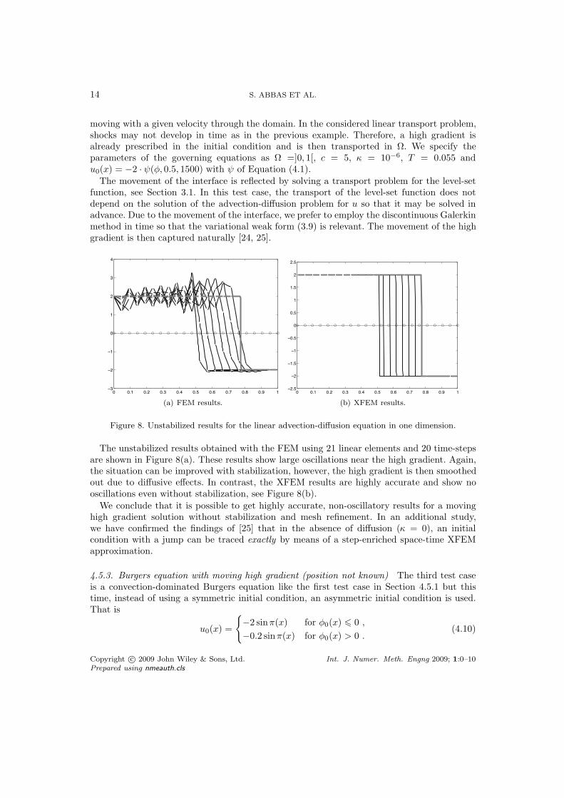
moving with a given velocity through the domain. In the considered linear transport problem,shocks may not develop in time as in the previous example. Therefore, a high gradient isalready prescribed in the initial condition and is then transported in #. We specify theparameters of the governing equations as # =]0, 1[, c = 5, # = 10"6, T = 0.055 andu0(x) = "2 · !(", 0.5, 1500) with ! of Equation (4.1).

The movement of the interface is reflected by solving a transport problem for the level-setfunction, see Section 3.1. In this test case, the transport of the level-set function does notdepend on the solution of the advection-di!usion problem for u so that it may be solved inadvance. Due to the movement of the interface, we prefer to employ the discontinuous Galerkinmethod in time so that the variational weak form (3.9) is relevant. The movement of the highgradient is then captured naturally [24, 25].

0 0.1 0.2 0.3 0.4 0.5 0.6 0.7 0.8 0.9 1−3

−2

−1

0

1

2

3

4

(a) FEM results.

0 0.1 0.2 0.3 0.4 0.5 0.6 0.7 0.8 0.9 1−2.5

−2

−1.5

−1

−0.5

0

0.5

1

1.5

2

2.5

(b) XFEM results.

Figure 8. Unstabilized results for the linear advection-di!usion equation in one dimension.

The unstabilized results obtained with the FEM using 21 linear elements and 20 time-stepsare shown in Figure 8(a). These results show large oscillations near the high gradient. Again,the situation can be improved with stabilization, however, the high gradient is then smoothedout due to di!usive e!ects. In contrast, the XFEM results are highly accurate and show nooscillations even without stabilization, see Figure 8(b).

We conclude that it is possible to get highly accurate, non-oscillatory results for a movinghigh gradient solution without stabilization and mesh refinement. In an additional study,we have confirmed the findings of [25] that in the absence of di!usion (# = 0), an initialcondition with a jump can be traced exactly by means of a step-enriched space-time XFEMapproximation.

4.5.3. Burgers equation with moving high gradient (position not known) The third test caseis a convection-dominated Burgers equation like the first test case in Section 4.5.1 but thistime, instead of using a symmetric initial condition, an asymmetric initial condition is used.That is

u0(x) =

*"2 sin((x) for "0(x) ! 0 ,

"0.2 sin((x) for "0(x) > 0 .(4.10)



Solution oftransport equation

Burgers equationSolution of

Burgers equationSolution of

Solution oftransport equation

tn+1tn

Figure 9. Strong coupling loop of the Burgers equation and the transport equation for the level-setfunction.

As a result, the position of the high gradient is now moving in time. This movement in timeis non-linear due to the non-linearity in the transport term of the Burgers equation. Onlythe initial position of the high gradient is given and described through "0(x) = x. As in theprevious test case, the movement of the highest gradient in time is captured by solving atransport problem for ". Other test case parameters are specified as # =]" 1, 1[, # = 5% 10"3

and T = 0.3.It is important to note the mutual dependence of the Burgers equation for u and the

transport equation for ". On the one hand, the result of the Burgers equation u e!ects theadvection velocity of the transport equation for ". On the other hand, the zero-level of " definesthe position of the largest gradient in the enrichment functions, so that the approximation spaceof the Burgers equation is e!ected by ". The mutual dependence of u and " leads to a coupledproblem in the sense of Felippa and Park [26, 27]. Here, we solve the coupled problem by astrong coupling loop of the two fields within each of the 80 time steps, see Figure 9.

The unstabilized solution for the FEM is shown in Figure 10(a) and large oscillations areobserved. In comparison, the XFEM solution in Figure 10(b) shows no oscillations. A space-time view of the problem is shown in Figure 10(c) where the curved line represents the zerolevel of the level-set function and is the position of the highest gradient. This figure shows thenon-linearity in the position of the highest gradient over time.

We conclude that the non-linear movement of the high gradient can be captured well so thatthe enrichment scheme stays e!ective throughout the simulation.

4.5.4. Advection-di!usion equation in two dimensions The fourth test case is an instationary,linear advection-di!usion problem in two dimensions where a scalar function is tranported ina circular velocity field. That is, the components of the velocity c are given as

cx = y " 0.5 and cy = "x + 0.5. (4.11)

The initial condition u0 is specified by (4.3) with & = 0.19h, where h is the mesh size. Thisinitial condition involves locally very high gradients but is constant in the major part of thedomain. Other test case parameters are specified as # =]0, 1[, # = 10"6 and T = 1.

A square mesh of 31 % 31 elements is used. For brevity, only the XFEM results are shownin Figure 11. No oscillations are observed for a rotation of the initial condition of 150% whichis realized in 200 time-steps. The three Figures 11(a) to (c) show the approximation at the


16 S. ABBAS ET AL.

−1 −0.8 −0.6 −0.4 −0.2 0 0.2 0.4 0.6 0.8 1−0.5

0

0.5

1

1.5

2

2.5

3

(a) FEM results.

−1 −0.8 −0.6 −0.4 −0.2 0 0.2 0.4 0.6 0.8 1−0.5

0

0.5

1

1.5

2

(b) XFEM results.

(c) XFEM results in the space-time domain. (d) XFEM results in the space-time domain.

Figure 10. Unstabilized results for the Burgers equation.

integration points after 1, 100 and 200 time steps, respectively. No oscillations are seen withoutany smoothing of the high gradient. The proposed enrichment scheme obviously extendsstraightforward to more than one spatial dimension.

5. XFEM for high gradients at the boundary (boundary layers)

Standard finite element approximations without stabilization also result into oscillatorysolutions for high gradients near the boundary (boundary layers). Typical meshes in fluidmechanics are highly refined near the boundary as these regions have an important influencein the ability of the approximation to capture the physics of a flow problem properly. Again,the aim is to define enrichment funtions for XFEM approximations that are able to obtainhighly accurate solutions without stabilization and mesh refinement. For a prescribed level ofaccuracy, a drastical decrease in the number of degrees of freedom is then expected for XFEMsimulations compared to FEM simulations on refined meshes near the boundary.

In many applications, boundary layers are not present along the whole boundary $ of



0 0.2 0.4 0.6 0.8 10

0.1

0.2

0.3

0.4

0.5

0.6

0.7

0.8

0.9

1

(a) Prescribed velocity field. (b) Solution at t = 1.

(c) Solution at t = 100. (d) Solution at t = 200.

Figure 11. Unstabilized XFEM results for the linear advection-di!usion equation in two dimensions.The high-gradient solution is plotted at the integration points in the domain.

the domain, for example, typically not at slip boundaries or at the inflow and outflow. Theenrichment is therefore only desired along selected parts of the boundary which is labelled$enr ) $. This is often the part of the boundary where no-slip boundary conditions areapplied.

An important di!erence to the situation considered in the previous section is that theposition of the highest gradient is now the boundary itself, so that the level-set method isnot needed for the definition of the enrichment functions. Instead, the enrichment functionsshould depend on the discretization near the wall. They are only mesh-dependent, i.e. theparameters of the governing equations are not used. A di!erent strategy would be to employonly one enrichment function and estimate the thickness of the boundary layer, e.g. in aniterative procedure. It is noted that, as long as the boundaries are fixed in space, the enrichmentfunctions for boundary layers are time-independent.


18 S. ABBAS ET AL.

Enrichment Function q Layer L!1 50 1!2 15 1!3 12 2!4 10 3

Table II. The set of 4 enrichment functions used for high gradients near the wall.

5.1. Optimal set of enrichment functions

We again start by finding an “optimal” set of enrichment functions. A similar procedure asdescribed in Section 4.2 is employed. The domain is again # =]0, 1[ and the di!erent functionsfor f(x) have high gradients at x = 1. We use functions f(x) of the kind xq, exp(q · x), andsinh(q · x), where the parameter q ' 1 ! R scales the gradient. The set of m enrichmentfunctions is based on

!(x, L) =exp(q · SL(x)) " 1

exp(q) " 1. (5.1)

The function SL(x) varies between 0 and 1 within L element layers of the wall for L = 1, 2, 3.They are defined by means of standard finite element shape functions:

S1(x) =!

i!J1

Ni(x), (5.2)

S2(x) =12

2 !

i!J2

Ni(x) + 2 ·!

i!J1

Ni(x)3

, (5.3)

S3(x) =13

2 !

i!J3

Ni(x) + 2 ·!

i!J2

Ni(x) + 3 ·!

i!J1

Ni(x)3

. (5.4)

The nodal set J1 is built by the nodes along the enriched boundary $enr, J2 are the nodes oneelement layer away from $enr, and J3 are the nodes two element layers away from $enr. Thesituation is depicted in Figure 12 in one and two dimensions.

The optimal set for 4 enrichment functions is given in table II. These enrichment functionsare visualized in two dimensions in Figure 13. For high gradients near boundaries, we find thatusing more enrichment functions does not improve the results noticeable. It is not su"cientto enrich only the nodes in the first element layer next to $enr, i.e. in this case, oscillations inthe approximated solution remain. Higher gradients than the one defined through !1 requirea very large number of integration points in the enriched elements and a!ect the conditioningof the system of equations unfavorably.

5.2. Quadrature

The high gradients in the enrichment functions require an accurate quadrature. Becausethe highest gradient is present near the boundary and thus aligns with the element edges,no decomposition into subelements for integration purposes is required. Therefore, we usestandard Gauss rules with a large number of integration points in the enriched elements. Theintegration points are then concentrated near the element edges where they are needed.



Figure 12. The functions SL and nodal sets JL in one and two dimensions. Note that each functionSL extends over L element layers near the enriched boundary.

5.3. Numerical examples with high gradients at the boundary

Three stationary convection-dominated problems are considered. The optimal set of fourenrichment functions described in Section 5.1 is used to enrich the approximation space. Theposition of the highest gradient is on the boundary $enr which is enriched.

5.3.1. Advection-di!usion equation in one dimension The stationary advection-di!usionequation in one dimension is considered first, the governing equations of Section 3.1 aremodified accordingly. The domain is # =]0, 1[ with boundary conditions u(0) = 0 and u(1) = 1.The exact solution is

uex(x) =exp(c/K · x) " 1exp(c/K " 1)

. (5.5)

Three di!erent ratios c/K are considered: c/K = {1, 20, 40} leading to a small, moderate,and high gradient at x = 1, see Figure 14. The number of linear elements n is varied from


20 S. ABBAS ET AL.

(a) (b)

(c) (d)

Figure 13. The resulting 4 enrichment functions in two dimensions for the domain shown in Figure12(c).

0 10

1

c/K = 1c/K = 20c/K = 40

Figure 14. The exact solutions for c/K = {1, 20, 40} leading to a small, moderate, and high gradientat x = 1, respectively.



10, 20, . . . , 640. The error in the L2-norm for the three di!erent c/K-ratios is shown in Figure15(a) for unstabilized XFEM and FEM results. For c/K = 1, the FEM and XFEM results are

10−2 10−1

10−6

10−4

10−2

100

element size h

L2−n

orm

c/K = 1. XFEMc/K = 20. XFEMc/K = 40. XFEMc/K = 1. FEMc/K = 20. FEMc/K = 40. FEM

(a)

0 100 200 300 400 5000

0.5

1

1.5

2

2.5

ratio c/K

max

imum

osc

illat

ion

n = 10,40,160. XFEMn=10. FEMn=40. FEMn=160. FEM

(b)

Figure 15. (a) Convergence in the L2-norm, (b) largest pointwise error (maximum oscillation) forXFEM and FEM approximations.

very similar over the whole range of elements. This shows that, as expected, the enrichmentis not needed for this case. For c/K = 20 and c/K = 40, on coarse meshes, the XFEM-resultsare drastically improved compared to the FEM results. For finer meshes, the XFEM resultsconverge to the FEM solution as the enrichment becomes less useful.

The largest pointwise error in the domain (maximum oscillation) over the whole range ofc/K ! ]0, 500[ for three di!erent numbers of elements n = {10, 40, 160} is studied in Figure15(b). It is seen that for the XFEM approximation no oscillations are observed up to c/K = 500even on the coarsest mesh. In contrast, the unstabilized FEM shows large pointwise errors thatincrease with c/K. It is thus seen that the proposed set of enrichment functions produces highlyaccurate results over the complete range of high gradients near the boundary.

5.3.2. Burgers equation in one dimension A similar study is repeated for the stationaryBurgers equation in one dimension. The domain is # =]" 1, 0[ and the exact solution is givenas

uex (x) = "2#s · exp(2sx) " t

exp(2sx) + twith s, t ! R. (5.6)

The Dirichlet boundary conditions are chosen such that Equation (5.6) is the exact solutionwith s = 20, t = 1, see Figure 16(a) and the di!usion parameter is set to # = 10"3.

Convergence results in the L2-norm are shown in Figure 16(b) for unstabilized XFEM andFEM approximations. The findings of the previous section are confirmed: On coarse meshesthe situation improves drastically with the extended approximation. We have also investigateddi!erent gradients at x = 0 and studied the maximum pointwise error. These results areomitted for brevity as they are very similar to the ones obtained in the previous test-case andlead to the same conclusions.

5.3.3. Advection-di!usion equation in two dimensions As a third text-case, the stationaryadvection-di!usion equation in two dimensions is considered. The domain # is a 90% segment


22 S. ABBAS ET AL.

−1 −0.8 −0.6 −0.4 −0.2 00

0.005

0.01

0.015

0.02

0.025

0.03

0.035

0.04

(a)

10−3 10−2 10−110−7

10−6

10−5

10−4

10−3

10−2

element size h

L2−n

orm

XFEMFEM

(b)

Figure 16. (a) The exact solution of the Burgers equation for " = 0.001, s = 20, t = 1, (b) convergencein the L2-norm for XFEM and FEM approximations.

spanned by r1 = 0.1 and r2 = 1.0 and is shown in Figure 17(a). The exact solution is

uex (x, y) =exp (cx/K · x + cy/K · y) " 1

exp (cx/K + cy/K) " 1. (5.7)

The boundary conditions are applied along $ accordingly. The gradient at $enr = {x : *x* =r2}, where * · * is the Euclidean norm, is scaled by the ratios of cx/K and cy/K. We choosecx = cy = c in this test case. The exact solution for c/K = 5 is shown in Figure 17(b).It is important to note that the solution involves a high gradients in normal direction tothe wall but only changes mildly along $enr. A typical opimized mesh for standard FEMcomputations would consist of high-aspects ratio elements along the boundary in order toresolve the boundary layer. However, for the computations considered in this work, the elementsize in normal direction is constant.

(a) (b)

Figure 17. (a) The domain #, (b) the exact solution of the advection-di!usion problem for c/K = 5.



A convergence study is carried out comparing the proposed set of enrichment functions witha standard FE approximation. In Figure. 18(a), for varying element numbers, the errors areshown in the L2-norm for di!erent c/k = {5, 20, 100}. Our findings in one dimensions areagain confirmed for this two-dimensional test case: On coarse meshes the accuracy is largelyimproved for the XFEM, on finer meshes, XFEM and FEM results converge to each other. Asan example, for c/K = 200, the same level of accuracy than the XFEM results on a 10 % 10mesh is obtained for the FEM with a uniformly refined mesh of 80% 80 elements.

10−2 10−1

10−4

10−2

100

element size h

L2−n

orm

c/K = 5. XFEMc/K = 20. XFEMc/K = 100. XFEMc/K = 5. FEMc/K = 20. FEMc/K = 100. FEM

(a)

0 20 40 60 80 1000

0.1

0.2

0.3

0.4

0.5

0.6

0.7

0.8

ratio c/K

max

imum

osc

illat

ion

n = 10,20,30. XFEMn=10. FEMn=20. FEMn=30. FEM

(b)

Figure 18. (a) Convergence in the L2-norm, (b) largest pointwise error (maximum oscillation) forXFEM and FEM approximations.

The largest pointwise error (maximum oscillation) is studied again. For di!erent mesheswith 10% 10, 20% 20, and 30% 30 elements the ratio c/K is varied in the range from 0 to 100,see Figure 18(b). As expected the FEM results worsen with increasing c/K ratio. The XFEMresults show again no visible oscillations. It is thus seen that although the enrichment functions!1 to !4 are constant in tangential direction of $enr, see Figure 13, the XFEM approximationis able to capture both, the large gradient in normal direction and the moderate change intangential direction of $enr.

6. Conclusions

An enrichment scheme for the XFEM has been proposed which enables highly accurateapproximations of convection-dominated problems without stabilization or mesh refinement.The high gradients inside the domain (shocks) and at the boundary (boundary layers) arecaptured by a set of enrichment functions used in the vicinity of the high gradients.

For high gradients in the domain, the enrichment functions are regularized step functionsthat depend on the distance from the shock. The position of the highest gradient is describedby the level-set function. Moving shocks are considered for by solving an additional advectionproblem for the level-set function. For high gradients at the boundary, exponential functionsare used as enrichment functions. They depend on the discretization along the boundary andno level-set function is needed. The enrichment for boundary layers is independent of time aslong as the boundary is fixed.


24 S. ABBAS ET AL.

The proposed enrichment scheme is independent of parameters in the governing equations.The whole set of enrichment functions was used in all test-cases, i.e. no iterative procedure isneeded in each time-step in order to determine only one suitable enrichment function.

The next step is to apply the proposed enrichment scheme to flow problems which areconvection-dominated in many problems of practical relevance. The results will be reported ina forthcoming publication.

ACKNOWLEDGEMENTS

Financial support from the Deutsche Forschungsgemeinschaft (German Research Association) throughgrant GSC 111 and the Emmy-Noether program is gratefully acknowledged.

REFERENCES

1. Belytschko T, Black T. Elastic crack growth in finite elements with minimal remeshing. Internat. J.Numer. Methods Engrg. 1999; 45:601 – 620.

2. Moes N, Dolbow J, Belytschko T. A finite element method for crack growth without remeshing. Internat.J. Numer. Methods Engrg. 1999; 46:131 – 150.

3. Elguedj T, Gravouil A, Combescure A. Appropriate extended functions for X-FEM simulation of plasticfracture mechanics. Comp. Methods Appl. Mech. Engrg. 2006; 195:501 – 515.

4. Gravouil A, Moes N, Belytschko T. Non-planar 3D crack growth by the extended finite element and levelsets, part II: level set update. Internat. J. Numer. Methods Engrg. 2002; 53:2569 – 2586.

5. Moes N, Gravouil A, Belytschko T. Non-planar 3D crack growth by the extended finite element and levelsets, part I: mechanical model. Internat. J. Numer. Methods Engrg. 2002; 53:2549 – 2568.

6. Karihaloo B, Xiao Q. Modelling of stationary and growing cracks in FE framework without remeshing: astate-of-the-art review. Computers & Structures 2003; 81:119 – 129.

7. Brooks A, Hughes T. Streamline upwind/Petrov-Galerkin formulations for convection dominated flowswith particular emphasis on the incompressible Navier-Stokes equations. Comp. Methods Appl. Mech.Engrg. 1982; 32:199 – 259.

8. Hughes T, Franca L, Hulbert G. A new finite element formulation for computational fluid dynamics: VIII.The Galerkin/least-squares method for advective-di!usive equations. Comp. Methods Appl. Mech. Engrg.1989; 73:173 – 189.

9. Donea J, Huerta A. Finite Element Methods for Flow Problems. John Wiley & Sons: Chichester, 2003.10. Hughes T, Brooks A. A multidimensional upwind scheme with no crosswind di!usion. ASME Monograph

AMD-34, vol. 34, Hughes T (ed.). ASME: New York, NY, 1979.11. Arnold DN, Brezzi F, Cockburn B, Marini LD. Unified analysis of discontinuous galerkin methods for

elliptic problems. SIAM J. Numer. Anal 2002; 39(5):1749 – 1779.12. Cockburn B, Shu C. The local discontinuous galerkin method for time-dependent convection-di!usion

systems. SIAM J. Numer. Anal 1998; 35(6):2440 – 2463.13. Patzak B, Jirasek M. Process zone resolution by extended finite elements. Eng. Fract. Mech. 2003; 70:957

– 977.14. Areias P, Belytschko T. Two-scale method for shear bands: thermal e!ects and variable bandwidth.

Internat. J. Numer. Methods Engrg. 2007; 72:658 – 696.15. Benvenuti E. A regularized XFEM framework for embedded cohesive interfaces. Comp. Methods Appl.

Mech. Engrg. 2008; 197:4367 – 4378.16. Waisman H, Belytschko T. Parametric enrichment adaptivity by the extended finite element method.

Internat. J. Numer. Methods Engrg. 2008; 73:1671 – 1692.17. Osher S, Fedkiw R. Level Set Methods and Dynamic Implicit Surfaces. Springer Verlag: Berlin, 2003.18. Sethian J. Level Set Methods and Fast Marching Methods. 2 edn., Cambridge University Press: Cambridge,

1999.19. Tezduyar T, Sathe S. Stabilization parameters in SUPG and PSPG formulations. J. Comput. Appl. Math.

2003; 4:71 – 88.20. Benvenuti E, Tralli A, Ventura G. A regularized XFEM model for the transition from continuous to

discontinuous displacements. Internat. J. Numer. Methods Engrg. 2008; 74:911 – 944.



21. Xiao Q, Karihaloo B. Improving the accuracy of XFEM crack tip fields using higher order quadrature andstatically admissible stress recovery. Internat. J. Numer. Methods Engrg. 2006; 66:1378 – 1410.

22. Bordas S, Nguyen P, Dunant C, Guidoum A, Nguyen-Dang H. An extended finite element library. Internat.J. Numer. Methods Engrg. 2007; 71:703 – 732.

23. Daux C, Moes N, Dolbow J, Sukumar N, Belytschko T. Arbitrary branched and intersecting cracks withthe extended finite element method. Internat. J. Numer. Methods Engrg. 2000; 48:1741 – 1760.

24. Fries T, Zilian A. On time integration in the XFEM. Internat. J. Numer. Methods Engrg. 2009; 79:69 –93.

25. Chessa J, Belytschko T. Arbitrary discontinuities in space-time finite elements by level-sets and X-FEM.Internat. J. Numer. Methods Engrg. 2004; 61:2595 – 2614.

26. Park K, Felippa C, Ohayon R. Partitioned formulation of internal fluid-structure interaction problems bylocalized lagrange multipliers. Comp. Methods Appl. Mech. Engrg. 2001; 190:2989 – 3007.

27. Felippa C, Park K, Farhat C. Partitioned analysis of coupled mechanical systems. Comp. Methods Appl.Mech. Engrg. 2001; 190:3247 – 3270.


Documents

The XFEM for high-gradient solutions in convection … Webseite...XFEM FOR CONVECTION-DOMINATED HIGH GRADIENT SOLUTIONS 1 In this paper, we focus on advection-dominated problems as