1

The World Distribution of Household Wealth

James B. Davies*, Susanna Sandstrom†, Anthony Shorrocks†, and Edward N. Wolff‡

5 December 2006

* Department of Economics

University of Western Ontario

London, Canada N6A 5C2

† UNU-WIDER

Katajanokanlaituri 6 B

00160 Helsinki, Finland

‡ Department of Economics

269 Mercer Street, Room 700

New York University

New York, NY 10003 USA

We thank participants at the May 2006 WIDER project meeting on Personal Assets from a

Global Perspective for their valuable comments and suggestions. Special thanks are due to Tony

Atkinson and Markus Jäntti. Responsibility for all errors or omissions is our own.

2

1 Introduction

Much attention has recently been focused on estimates of the world distribution of income

(Bourguignon and Morrison, 2002; Milanovic, 2002 and 2005). The research shows that the

global distribution of income is very unequal and the inequality has not been falling over time. In

some regions poverty and income inequality have become much worse. Interest naturally turns to

the question of global inequality in other dimensions of economic status, resources or wellbeing.

One of the most important of these measures is household wealth.

In everyday conversation the term ‘wealth’ often signifies little more than ‘money income’. On

other occasions economists interpret the term broadly and define wealth to be the value of all

household resources, both human and non-human, over which people have command. Here, the

term is used in its long-established sense of net worth: the value of physical and financial assets

less liabilities.1 Wealth in this sense represents the ownership of capital. While only one part of

personal resources, capital is widely believed to have a disproportionate impact on household

wellbeing and economic success, and more broadly on economic development and growth.

Wealth has been studied carefully at the national level since the late nineteenth or early twentieth

centuries in a small number of countries, for example Sweden, the UK and the US. In some other

countries, for example Canada, it has been studied systematically since the 1950s. And in recent

years the number of countries with wealth data has been increasing fairly quickly. The largest

and most prosperous OECD countries all have wealth data based on household surveys, tax data

or national balance sheets. Repeated wealth surveys are today also available for the two largest

developing countries — China and India, and a survey that inquired about wealth is available for

Indonesia. Forbes magazine enumerates the world’s US$ billionaires and their holdings. More

detailed lists are provided regionally by other publications, and Merrill-Lynch estimate the

number and holdings of US$ millionaires around the world. National wealth has been estimated

1 In some work attempts have been made to include ‘social security wealth’, that is the present value of expected net benefits from public pension plans in household wealth. We exclude social security wealth here, in part because estimates are available for only a few countries.

3

for a large number of countries by the World Bank.2 In short, there is now an impressive amount

of information on wealth holdings. We believe the time has therefore come to estimate the world

distribution of household wealth.3

In this paper we show, first, that there are very large intra-country differences in the level of

household wealth. The US is the richest country, with mean wealth estimated at $144,000 per

person in the year 2000.4 At the opposite extreme among countries with wealth data, we have

India with per capita wealth of about $6,500 in purchasing power parity (PPP) terms. Other

countries show a wide range of values. Even among high income OECD countries there is a

range from figures of $56,000 for New Zealand and $66,000 for Denmark to $129,000 for the

UK (again in PPP terms).

We also look at international differences in the composition of wealth. There are some

regularities but also country-specific differences — such as the strong preference for liquid

savings in a few countries, such as Japan. Real assets, particularly land and farm assets, are more

important in less developed countries. This reflects not only the greater importance of

agriculture, but a lack of financial development that is being corrected in some of the most

rapidly growing LDCs. Among rich countries, financial assets and share-holding tend to bulk

largest in those with more reliance on private pensions and/or the most highly developed

financial markets, such as the UK and US

The concentration of wealth within countries is high. Typical Gini coefficients in wealth data lie

in the range of about 0.65 - 0.75, while some range above 0.8. In contrast, the mid-range for

2 See World Bank (2005). National wealth differs from household wealth in including the wealth of all other sectors, of which corporations, government and the rest-of-the-world are important examples.

3 One sign of the growing maturity of household wealth data is the launching of the Luxembourg Wealth Study (LWS) parallel to the long-running Luxembourg Income Study (LIS). See http://www.lisproject.org/lws.htm. In its first phase the LWS aims to provide comparable wealth data for nine OECD countries, with the cooperation of national statistical agencies or central banks. The LWS initiative differs from ours in that its aim is not to estimate the world distribution of wealth, but to assemble fully comparable wealth data across an important subset of the world's countries.

4 All our wealth estimates are for the year 2000. Wealth data typically become available with a significant lag, and wealth surveys are conducted at intervals of three or more years. The year 2000 provides us with a reasonably recent date and good data availability.

4

income Ginis is from about 0.35 – 0.45. The mid value for the share of the top 10 per cent of

wealth-holders in our data is 50 per cent, again higher than is usual for income.

While inter-country differences are interesting, our goal is to estimate the world distribution of

wealth. In order to do so we need estimates of the levels and distribution of wealth in countries

where data on wealth are not available. Fortunately for our exercise, the countries for which we

have data included 56 per cent of the world’s population in the year 2000 and, we estimate, more

than 80 per cent of its household wealth. Careful study of the determinants of wealth levels and

distribution in the countries that have wealth data allows imputations to be made for the ‘missing

countries’.

The remainder of the paper is organized as follows. In the next section we study what can be

learned about household wealth levels and composition across countries using household balance

sheet and survey data. Section 3 presents our empirical results on the determinants of wealth

levels, and imputes household wealth totals to the ‘missing countries’. Section 4 reviews

evidence on the distribution of wealth where available, and then performs imputations for other

countries. In Section 5 levels and distributions are combined to construct the global distribution

of household wealth. Conclusions are drawn in Section 6.

2 Wealth Levels

Our objective in this section is to develop data on measured wealth levels in as many countries as

possible. These data are of independent interest, but are also used in the next section to impute

per capita wealth to a large sample of countries that do not have wealth data. The exercise begins

by taking inventories of household balance sheet (HBS) and sample survey estimates of

household wealth levels and composition. Sources and Methods for HBS data are detailed in

Appendix I, and sources of survey data are shown in Appendix III.

A Household Balance Sheet (HBS) Data

We have assembled balance sheets for as many countries as possible. As indicated in Table 1,

‘complete’ financial and non-financial data are available for 18 countries. These are all high

income countries, except for the Czech Republic, Poland, and South Africa, which are upper

5

middle income countries.according to the World Bank classification.5 We considered the data

complete if there was full or almost full coverage of financial assets, and inclusion at least of

owner-occupied housing on the non-financial side. There are 15 other countries that have

comparable financial balance sheets, but no information on the real side. Here there is better

representation outside the high income countries, with six upper middle income countries and

three lower middle income.

Country coverage in HBS data is not representative of the world as a whole. Such data tend to be

developed at a relatively late stage in the development of national economic statistics. Europe

and North America, and the OECD in general, are well covered, but low income and transition

countries are not.6 In geographic terms this means that coverage is sparse in Africa, Asia, Latin

America and the Caribbean. Fortunately for this study, these gaps in HBS data are offset to an

important extent by the availability of survey evidence for the largest developing countries,

China, India and Indonesia, as discussed below. Also note that while there are no HBS data for

Russia, we do have complete HBS data for two European transition countries and financial data

for eight others.

Table 2 summarizes key characteristics of the household balance sheet data by country. As

discussed in Appendix I, methods and sources differ across countries. This is especially true for

non-financial assets. Often, the balance sheets are compiled in conjunction with the National

Accounts or Flow of Funds data, but there are several exceptions. For countries such as New

Zealand, Portugal and Spain, data are reported by central banks and include estimates based on

Financial Accounts augmented with data on housing assets. The German and Italian data are to a

large extent also based on central bank data but are more complete. The German data are based

on Financial Accounts data from Deutsche Bundesbank and non-financial assets data including

5 We used the World Bank classification throughout the paper except that Brazil, Russia and South Africa were moved from the lower middle income category to higher middle income, and Equatorial Guinea from low to lower middle income. We made these changes since the WB classifications seemed anomalous on the basis of the Penn World Table GDP data that we use for year 2000.

6 Goldsmith (1985) prepared ‘planetary’ balance sheets for 1950 and 1978 and found similar difficulties in obtaining representative coverage. He was able to include 15 developed market economies, two developing countries (India and Mexico), and the Soviet Union. This produces a total of 18 countries, equal in number to the countries for which we have complete HBS data for the year 2000.

6

housing assets, other real assets and durables. The Italian data are based on the Financial

Accounts from the Bank of Italy augmented with Italian statistical office (Istat) estimates of the

stock of dwellings and calculations of durable goods based on Istat data by Brandolini et. al

(2004). Even if the household balance sheets are based on data from the national statistical

organizations they do not necessarily have a broad coverage of non-financial assets. The data for

the Netherlands are a mix of data from Statistics Netherlands and the central bank, and the

financial balance sheets are only augmented with data on owner-occupied housing. The non-

financial data from the Singapore Department of Statistics also covers only housing assets. For

Denmark we combined financial balance sheet data with fixed capital stock accounts reported by

Statistics Denmark.

Summarizing, each of the 18 countries we have classed as having complete balance sheets have

good financial data plus some information on housing. Poland, Singapore and the Netherlands

are at this minimum level. Fifteen countries report data on some other real property, including

land and/or investment real estate in most cases, and six have estimates for consumer durables.

We considered whether we could make imputations that would make the non-financial coverage

in these ‘complete’ balance sheets more uniform. We found that it would be very difficult to do a

satisfactory imputation for land or investment real estate.7 We have therefore not imputed these

items. Since only three countries are completely missing these items and eight countries,

including the US have complete data, we believe that while gaps for these items do have some

effect on our results, the impact should not be exaggerated. In contrast, it is possible to do a

reasonable imputation for consumer durables. Since this improves estimates for twelve countries,

we included these imputations.8

7 While the value of land occupied by included dwellings is captured in the balance sheets, other land is missing for Denmark, Germany, Italy, the Netherlands, and Singapore. Investment or commercial real estate is missing for the Netherlands, New Zealand, Portugal and Singapore, and for Italy (for which all housing is included, whether owner occupied or not, but not other real estate). To the best of our knowledge, in all other cases both land and all real estate owned by households are included in the data specification.

8 Durables data are available for Canada, the US, Germany, Italy and South Africa. We used the mean ratio of durables to GDP in Canada and the US to impute durables to Australia, New Zealand, and the UK. For European countries other than the UK we used the mean ratio for Germany and Italy. Finally, the mean ratio for Canada, the US, Germany and Italy was used to do the imputation for Japan and Singapore.

7

Table 2 also shows that there are differences in sectoral definition across countries. We aimed for

a household sector which covered the assets and debts of households and unincorporated

business. However, non-profit organizations (NPOs) are sometimes grouped in with households.

We would like to exclude NPOs, and had data allowing us to do so for the UK and US. This

correction is especially important for the US where NPOs account for about 6 per cent of the

financial assets of the household sector (Board of Governors of the Federal Reserve System,

2003).

Table 3 reports the asset composition of household balance sheets. The asset composition reflects

different influences on household behaviour such as market structure, regulation and cultural

preferences (IMF, 2005). One needs, however, to be careful when analyzing these data since the

comparison may be affected by sectoral definition, asset coverage and methodological

differences. For most countries, non-financial assets account for between 40 and 60 per cent of

total assets, with higher shares in the Czech Republic, New Zealand, Poland and Spain. Housing

assets constitute a considerable share of non-financial assets. In the United Kingdom and some

other countries, the large increase in real estate prices in the late 1990’s helps to explain a high

housing share. The high share of financial assets makes South Africa stand out. One would

expect real assets like housing, land, agricultural assets and durables to be important in a

developing country, but due to well developed financial markets combined with continuously

negative rates of return on investment in fixed property and relatively high mortgage interest

rates, the share of non-financial assets is unusually low in South Africa (see Aron et al., 2006).

The United States is also an outlier in the share of financial assets, which is clearly related to the

strength of its markets, but may also be partly explained by its relatively cheap housing.

Turning to the composition of financial assets, we can draw on the 15 countries for which we

have financial balance sheets only, in addition to the 18 with complete balance sheets. There are

some striking differences across countries. We disaggregate into liquid assets, shares and

equities, and other financial assets. In Japan and most of the European transition countries, liquid

8

assets are a large part of the total.9 In transition countries this is expected due to poorly

developed financial markets. In Japan the preference for liquidity has a long history but also

reflects lack of confidence in real estate and shares after their poor performance in the 1990’s

(Babeau and Sbano, 2003). In some countries, such as Australia, Austria, the Netherlands, South

Africa and the UK the share of other financial assets is particularly high. This may be partly

attributable to the importance of pension fund claims in these countries. Italy stands out as

having a particularly low share of liabilities, something that is confirmed by survey data (see

below).

B Survey data

In order to check on our HBS data and to expand our sample, especially to non-OECD countries,

we also consulted household wealth survey data. Table 4 shows there is more variation in

country coverage than in the HBS data. Most importantly, wealth surveys are available for the

three most populous developing (and emerging market) countries: China, India and Indonesia.

These three countries, together with Finland, and Mexico in the case of non-financial assets, are

used in regressions in the next section that provide the basis for wealth level imputations for our

‘missing countries’.

Like all household surveys, wealth surveys suffer from sampling and non-sampling errors. These

are typically more serious for estimating wealth distribution than e.g. for income distributions.

The high skewness of wealth distributions makes sampling error more severe. Non-sampling

error is also a greater problem since differential response (wealthier households less likely to

respond) and misreporting are generally more important than for income. Both sampling and

non-sampling error lead to special difficulties in obtaining an accurate picture of the upper tail,

which is of course one of the most interesting parts of the distribution (see Davies and Shorrocks,

2000 and 2005).

9 Among the transition countries, shares of liquid assets in total financial assets are 60 per cent or higher for Bulgaria, the Czech Republic, Croatia, Romania, and Slovakia. Estonia and Lithuania stand out as having liquid asset shares of one-third or lower. Latvia, Hungary and Slovenia are intermediate between these extremes.

9

In order to offset the effects of sampling error in the upper tail, well-designed wealth surveys

over-sample wealthier households. This is the practice in the US Survey of Consumer Finances

and the Canadian Survey of Financial Security, for example.10 Among the four countries whose

survey data are used in the regressions reported in the next section, however, only Finland over-

samples rich households. Sampling error may therefore be of some concern in the Chinese CASS

survey, the Indian AIDIS survey (part of the Indian National Sample Survey round 59) and the

Indonesian Family Life Survey. This is despite very high reported response rates (in excess of 90

per cent) in both China and India. In the case of the Chinese survey, there are additional

difficulties regarding the representativeness of the wealth survey sub-sample, which covers only

a part of the provinces included in the sample of the State Statistical Bureau Household Income

Survey. The SSB sample itself also suffers from some degree of geographical under-coverage

(Bramall, 2001). The Indonesia Family Life Survey also has some coverage limitations. The

survey is reported to be representative of 83 per cent of the Indonesian population covering 13 of

the nation’s 27 provinces.

As mentioned above, non-sampling errors include both differential response by wealth level and

misreporting (mostly under-reporting). Wealthy households are less likely to respond to surveys.

As found here, comparisons with HBS data generally show lower totals for most financial assets

in surveys. This may be due to differential response and/or under-reporting by those who do

respond.11 In contrast, non-financial assets, especially housing, are sometimes better covered in

survey data. In terms of asset coverage the Finnish survey concentrates on financial assets,

housing and vehicles. The surveys from the three developing countries pay relatively little

attention to financial wealth since it is of less importance there, and concentrate on housing,

agricultural assets, land and consumer durables. The asset coverage and details of the surveys

reflect the relative importance of specific assets in rich and relatively poor countries.

10 The SCF design explicitly excludes people in the Forbes 400 list of the wealthiest Americans, which again helps to reduce the effects of sampling error. See Kennickell (2004).

11 Also, certain assets and liabilities in the balance sheets for the household sector are often computed as a residual, after the balance sheets for the government and corporate sector are first computed. The total asset values for the household sector are then given as the difference between total national wealth and the sum of these two other sectors, as in the US Flow of Funds. As a result, balance sheet totals for the household sector are also prone to error.

10

Table 4 reports asset composition in the survey data. It is clear that non-financial assets bulk

larger in surveys than in HBS data, reflecting both the relative accuracy of housing values in

survey data and the importance of under-reporting and non-response among rich households,

who own a disproportionate share of financial assets. The table also shows how different is the

importance of non-financial and financial assets in developed and developing countries. The two

low income countries in our sample, India and Indonesia, stand out as having particularly high

shares of non-financial wealth.12 This is no surprise since assets such as housing, land,

agricultural assets and consumer durables are particularly important in many developing

countries. In addition, financial markets are often poorly developed. In India, the only low or

middle income country for which we have some detail on financial assets, most of the financial

assets owned by households are liquid. Renwei and Sing (2005) report more detailed data for

urban areas of China, showing that about 64 per cent of household financial assets there are

liquid. In our table, China does not stand out as having high shares of non-financial assets. One

reason is that the value of housing is reported net of mortgage debt in China. Another is that

there is no private ownership of urban land. In addition, according to Renwei and Sing (2005),

there has been a rapid increase of financial assets especially in rural areas, reflecting the

deepening of market oriented reforms.

The ratio of liabilities to total assets is particularly low in India and Indonesia (for China only

non-housing liabilities are reported). Again poorly developed financial markets help to explain

this phenomenon. But, in addition, underreporting of debt appears to be more severe than

underreporting of assets. Subramanian and Jayaraj (2006) estimate that debts are, on average,

underrepresented by a factor of 2.93 in the AIDIS. Italy also stands out as having a very low

share of liabilities. This low share echoes the finding in HBS data, and likely reflects a real

difference between Italy and other high income OECD countries.

12 This echoes the findings of Goldsmith (1985) who reported that India and Mexico had an average of 65.0 per cent of national assets in tangible form in 1978, vs. 50.8 per cent for fourteen developed market economies.

11

C Per Capita Wealth from Household Balance Sheet and Survey Data

Table 5 summarizes the distribution of per capita wealth in the year 2000 among countries for

which we have complete household balance sheet and/or wealth survey data. (Data for individual

countries are given in Appendix IV.) The data are given both on PPP and official exchange rate

bases.

Of the 18 countries for which we have complete HBS data, the US ranks first on a PPP basis

(although it is surpassed by Japan at official exchange rates), with per capita wealth of $143,727

in 2000, followed by the UK at $126,832, Japan at $124,858, the Netherlands at $120,086, Italy

at $119,704, and then Singapore at $113,631. South Africa is last, at $16,266, preceded by

Poland at $24,654 and the Czech Republic at $32,431. The overall range is rather large, with per

capita wealth in the US 8.8 times as great as that of South Africa on the PPP basis. Differences

are even greater on an exchange rate basis, with the US/South Africa ratio rising to 24.0. The

coefficient of variation (CV), among the 18 countries rises from 0.427 on a PPP basis to 0.594 on

the exchange rate basis.

The next column shows GDP per capita. In the group of 18 countries with HBS data, the US

again ranks first, at $35,619, and South Africa last, at $8,017 on a PPP basis. However, the range

is much smaller than for net worth per capita. The ratio of highest to lowest GDP per capita is

only 4.4, and the (unweighted) coefficient of variation of GDP per capita (again among the 18

countries) is 0.311, compared to 0.427 for net worth per capita. On the exchange rate basis the

CV of GDP per capita is 0.519, compared to the 0.594 figure for wealth. These results are a first

illustration of the fact that, globally, wealth is more unequally distributed than income. The

comparison here is only between countries. The full results we present later in the paper include

inequality within countries, which further increases the gap between income and wealth

inequality.

In column 4 we show personal disposable income per capita for the same group of countries.

The US again ranks first, at $25,480, South Africa is again last, at $4,691 on a PPP basis, and the

ratio of highest to lowest is 5.4, slightly higher than for GDP per capita. The coefficient of

variation is 0.326, again slightly higher than that of GDP per capita. The last column shows real

consumption per capita. Once again, the US ranks first and South Africa last, the ratio of highest

12

to lowest on a PPP basis is 4.7, about the same as GDP per capita and slightly higher than that of

disposable income per capita. The CV is 0.319, slightly higher than that of GDP per capita and

slightly lower than that of disposable income per capita. On the exchange rate basis inequality

between countries is again greater than on a PPP basis. All in all, the variation of net worth per

capita is much greater than GDP per capita, disposable income per capita, and consumption per

capita.

The difference between countries is even more pronounced in the survey data results than in the

HBS data, due to the inclusion of three developing countries (China, India and Indonesia). Of the

13 countries for which we have the pertinent data, the US again ranks first in net worth per

capita, at $143,857, followed on a PPP basis by Australia at $101,597, and Japan at $91,856. In

this group, India is last, at $6,513 on a PPP basis and $1,112 on an exchange rate basis, preceded

by Indonesia, at $7,973 on a PPP basis and $1,440 using official exchange rates. China appears

to be about twice as wealthy as India, having per capita net worth of $11,267 on a PPP basis or

$2,613 using official exchange rates.

In the survey data, as in the HBS data, the range in per capita wealth is much larger than that of

per capita GDP, disposable income, or consumption. The ratio of highest to lowest is 22.1 for net

worth per capita, 13.3 for both GDP and disposable income, and 17.3 for consumption on a PPP

basis. Again, the coefficients of variation for the income and consumption variables are smaller

than for wealth, and inequality is considerably greater using official exchange rates rather than

PPP.

Wealth per capita is closely related to both income per capita and consumption per capita. The

correlation between net worth and GDP is only 0.739 in the HBS data on a PPP basis, but that

correlation rises to 0.848 on an official exchange rate basis, and is higher again in the survey data

— at 0.908 on an exchange rate basis (see Table 6). Correlations of wealth and disposable

income are higher from both HBS and survey sources — rising to 0.958 in the survey data on an

exchange rate basis. Correlations of wealth with consumption are a little lower: 0.860 from

balance sheet data and 0.922 from survey data, again on an exchange rate basis. The highest

correlations are between the logarithm of net worth per capita and the logarithm of disposable

income per capita: 0.975 from the balance sheet data and 0.993 from the survey data using

13

official exchange rates. Correlations of the logarithm of net worth per capita and the logarithm of

consumption per capita are slightly lower.

3 Imputing per Capita Wealth to other Countries

We next impute per capita wealth to the remaining countries of the world. For a large number of

countries part or all of wealth is imputed on the basis of regressions run on the 38 countries for

which we have HBS or survey data, as detailed below. This gives us 150 countries with observed

and/or imputed wealth, covering 95.2 per cent of the world’s population in 2000. It is tempting to

regard the results as representing the global picture. However this would implicitly assume that

the 79 excluded countries and people are neither disproportionately rich or poor. This assumption

is untenable. While the omitted countries include several smaller rich nations (for example,

Liechtenstein, the Channel Islands, Kuwait, Bermuda), the most populous countries

(Afghanistan, Angola, Cuba, Iraq, North Korea, Myanmar, Nepal, Serbia, Sudan and Uzbekistan

each have more than 10 million population) are all classified as low income or lower middle

income. To try to compensate for this bias, to each of the omitted countries we assign the mean

per capita wealth of the continental region (6 categories) and income class (4 categories).13 This

assumption is admittedly crude, but nevertheless an improvement over the default of simply

disregarding the excluded countries. It allows us, in the end, to assign wealth levels to 229

countries.

The regressions we report below are designed to help us predict wealth in countries where wealth

data are missing. The goal is not to estimate a structural model of wealth-holding, but to find

equations that fit well in-sample and that will also allow us to predict out-of-sample. The nature

of this exercise limits the range of models that can be applied. Perhaps most importantly, it limits

our choice of explanatory variables to those that are available not only for the countries with

wealth data but also for a large number of countries without wealth data.

13 Middle income Oceania was assigned a simple average of Fiji and New Zealand.

14

A Wealth Regressions

We first experimented with OLS regressions for those countries with complete wealth data,

excluding the 16 countries with incomplete data shown in Table 1. Initially our dependent

variable was simply per capita wealth. The principle independent variable was per capita income

or consumption. As Figures 1 and 2 make evident, there is a strong relationship between wealth

and income, so these equations fit fairly well.14 However, we discovered that we could predict

better if we disaggregated wealth into (i) non-financial assets, (ii) financial assets and (iii)

liabilities, and ran separate regressions for each. Part of the reason this approach yields better

results is that some variables are helpful in predicting one or two of these components, but not all

three. Also, the relative impacts of common variables vary across the equations. There are

significant gains from the greater flexibility offered by running separate regressions.

Having discovered that the results improved when we ran three regressions, we realized that

productive use could be made of data from countries where some, but not all three, components

were available. For the 15 countries shown in Table 1 with financial balance sheets, but no data

on real assets, there are observations of both financial assets and liabilities. And for Mexico, we

have an observation of non-financial assets. Adding observations from these countries has a

benefit not only in increasing sample size, but in bringing in more developing and transition

countries. The regressions therefore become better at predicting wealth for the ‘missing

countries’.

For our dependent variables we use the household balance sheet data discussed above for 33

countries, and survey data for five countries that lack HBS data (China, Finland, India,

Indonesia, and Mexico). In each regression the income variable is very important. The best fit is

obtained using disposable income per capita. We show the results of those runs in Appendix II.

Here we highlight runs using real consumption per capita instead, since this variable is available

for about twice as many countries as disposable income, which makes the consumption

14 Figure 1 uses wealth from the HBS data while Figure 2 uses wealth from survey data. The slopes of the simple regression lines in the two figures are similar, but the intercept is higher with HBS data. This reflects the fact that survey data generally provide lower estimates of wealth than national balance sheets.

15

specification far more useful for imputations. Using consumption reduces goodness of fit only

slightly.

Since errors in our three equations are likely to be correlated we investigated using the seemingly

unrelated regressions (SUR) technique due to Zellner (1962).15 This involves stacking the three

equations and estimating via generalized least squares. While OLS estimates would be

consistent, SUR provides greater efficiency. The gain in efficiency is expected to be greater the

more highly correlated are the errors across the equations, and the less correlated are the

regressors used in the different equations. For equations with an equal number of observations it

is straightforward to apply SUR in STATA. The results we show here for the financial assets and

liabilities regressions are therefore performed using SUR.16

Table 7 shows our results with three different versions of the consumption specification, labelled

a through c. Our preferred specifications are b for non-financial wealth and c for financial wealth

and for liabilities. Variable sources are given in Appendix II. Both the dependent variables and

most of the independent variables are entered in log form. Note first that real consumption per

capita appears significant at the 1 per cent level in all of the runs. The estimated elasticities of

non-financial and financial wealth with respect to consumption are 1.028 and 1.177 respectively

in our preferred runs. The slightly greater elasticity for financial wealth seems plausible, since

higher income countries tend to have better developed financial markets. There is an even larger

difference for liabilities, which have an estimated elasticity of 1.487. These differences imply

that, for the many low income countries where we make imputations, there will be a tendency

coming from the consumption variable for their imputed financial assets and (especially)

liabilities to be relatively less important than their non-financial assets.

15 See also Greene, 1993, pp. 486-499.

16 While it is theoretically possible to apply SUR with an unequal number of observations in the equations estimated, this is very difficult to do in STATA or (we expect) in other standard packages. Also, while errors in the financial assets and liabilities equations are likely to be correlated, this is less likely in comparing either of those variables with non-financial assets. Estimates of the latter generally come from different sources and are prepared using different techniques from those used in financial balance sheets. Thus correlations in measurement error, at least, should be small.

16

We tried a dummy variable indicating the data source (HBS or survey data) in all three

regressions. It was insignificant in the regression for non-financial assets, which is not

unexpected since survey data typically cover non-financial assets quite well. While significant at

the 10 per cent level in the first liabilities specification, it loses significance in the b specification

and was dropped from the final run. In contrast, the survey dummy is significant at the 1 per cent

level in all three runs for financial wealth. With a value of -1.516 in the c run, this dummy

reflects the well-known fact that financial assets are under-reported and under-represented in

survey data.

We also considered five other independent variables:

Population Density: The value of non-financial assets, particularly housing, should be

positively related to the degree of population density (greater density indicating a relative

scarcity of land). This variable is statistically significant in the non-financial asset regressions.

Market Capitalization Rate: The value of household financial assets should be positively

correlated with this measure of the size of the stock market. It is positive and significant in all

three regressions for financial wealth. This is a useful result in terms of prediction and

imputations, since the variable is available for a large number of countries that do not have

full wealth data.

Public Spending on Pensions as a Percentage of GDP: We expected this might be negatively

related to financial assets per capita, since public pensions may substitute for private saving.

However, this variable is not statistically significant and was dropped.

Income Gini: Some theoretical models suggest that income inequality and per capita wealth

should be positively related. However, the variable turns out to be insignificant.

Domestic Credits Available to the Private Sector: This variable is highly significant in the

liabilities regression, which is fortunate from the imputation perspective since, as in the case

of market capitalization, the variable is available for many of our ‘missing countries’.

The R2 or ‘R2’ for each equation indicates that we get a fairly good fit for our model.17

17 R2 is not a well-defined concept in generalized least squares, so as is customary the fraction of the variance in the dependent variable that is ‘explained’ in each regression is referred to as ‘R2’ here.

17

B Imputations

Table 8 shows summary results for our full sample of 229 countries. We again grouped countries

into (i) high income OECD; (ii) high income non-OECD; (iii) upper middle income; (iv) lower

middle income; and (v) low income classes, and present information here for groups only. A

complete list of estimated wealth by country is provided in Appendix V.

Looking first at the 24 high income OECD countries, on a PPP basis we find a share of world

household wealth of 63.7 per cent, much larger than this group’s 14.8 per cent share of world

population and significantly more than its 53.6 per cent share of world GDP. Thus we have an

immediate indication of the high concentration of world wealth in the richest countries, and a

strong indication that wealth is more unequally distributed across countries than is income. The

degree of concentration is even greater if the calculations are done on an official exchange rate

basis. The high income OECD countries then have 83.3 per cent of world household wealth (and

76.9 per cent of world GDP); and as we found above for countries with HBS or survey data, the

CV of per capita wealth is much higher when we measure wealth on an exchange rate basis.

While it is natural to compare wealth levels across countries in terms of wealth per capita, other

options may also have attractions. In particular, there is a case for expressing wealth levels in

terms of the average wealth per family (or household) or the average wealth per adult, the latter

reflecting an implicit assumption that the wealth holdings of those under 20 years of age can be

neglected in global terms. The choice between the three alternative concepts becomes more

significant in the context of wealth distribution, and is discussed in more detail in Section 5

below. Here we simply note that computing average wealth per household poses practical

problems, since the total population of households is not reported for many countries. In contrast,

the number of adults (specifically, the number of persons aged 20 or above) is widely available.

We therefore provide a second set of figures for the average wealth per adult in each country.18

18 When the population over 20 is not reported, we imputed estimates based on the average proportion of adults in the region-income category used previously. Imputed levels of wealth per adult use regional averages weighted by the number of adults rather than the total population.

18

Table 8 shows that for the high income OECD countries wealth per adult is about a third higher

than wealth per capita ($151,308 vs. $113,675 in PPP results). Larger proportional differences

are found for lower income countries, where adults comprise a smaller fraction of the population.

Wealth inequality among these high income OECD countries is higher on a per adult basis than

on a per capita basis, but the difference is quite small.

For the high-income non-OECD and upper middle income groups we again find that wealth

inequality tends to be greater than income inequality, and that both wealth and income inequality

between countries are higher within the group when we use official exchange rates rather than

PPP. (There is no systematic difference between wealth inequality on a per adult vs. per capita

basis.) However, for the 59 lower middle income and 64 low income countries we find different

results. In both cases per capita wealth inequality is less than inequality in per capita GDP

according to our estimates.19 And for the low income countries inequality is greater on a PPP

basis than when using official exchange rates (true for both wealth and GDP).

On a PPP basis the 43 countries in the high-income non-OECD group accounted for 3.23 per

cent of world household wealth and 2.35 per cent of world GDP, while having just 0.93 per cent

of world population. These countries include many small but wealthy countries, for example the

Bahamas, Bahrain, Taiwan, Israel, Kuwait, Qatar, Singapore, and the United Arab Emirates.

Average PPP-based per capita wealth for the whole group was 3.5 times the average for the

world. This group too showed greater inequality in per capita wealth than in per capita GDP

(CVs of 0.484 and 0.184, respectively on a PPP basis).

The 39 countries in the upper middle-income group had an average wealth just a little below the

world average. This group includes countries like Brazil, Mexico, Poland and Russia. Poland’s

per capita wealth was close to the world average, while Mexico and Brazil were somewhat lower

(81 per cent and 80 per cent respectively on a PPP basis), and Russia stood at 67 per cent of the

world mean. (See Appendix V where full details are given for all countries.) Each of these

countries had a smaller share of world wealth than of world GDP — in the case of Russia 1.6 per

19

cent of the wealth vs. 3.2 per cent of world GDP. Overall, the upper middle-income group

accounted for 9.2 per cent of the world household (PPP) wealth, 11.4 per cent of the world

population but 13.9 per cent of world GDP. This group also showed greater inequality in per

capita wealth than in per capita GDP (CVs of 0.277 and 0.170, respectively, on a PPP basis).

The lower middle income group includes China, Egypt, Turkey, and the Ukraine. According to

our estimates, some of these countries, like Turkey, have a larger share of world wealth than of

world GDP. Others, like Egypt and the Ukraine, have a smaller share of wealth than of GDP.

However, it is interesting to note that China, which is such an important element in the world

distribution, has fairly similar shares of world wealth and GDP, at least on a PPP basis: 8.8 per

cent of world household wealth and 10.5 per cent of world GDP. (However, according to official

exchange rates, its wealth share is only 2.6 per cent and its GDP share is 3.5.) The collective

household wealth of the 59 lower middle income countries amounted to 15.5 per cent of the

world total on a PPP basis. This compares to their 33.0 per cent share of world population and

their 18.9 per cent of world GDP on a PPP basis. Interestingly, for this group the inequality of

per capita wealth fell short of its inequality of GDP per capita (CVs of 0.240 and 0.264,

respectively).

The last group consists of 64 low-income countries. Its collective household net worth on a PPP

basis amounted to 8.3 per cent of world wealth, compared to 39.9 per cent of the world’s

population and 11.3 per cent of world GDP. This group consists of countries such as India,

whose average per capita net worth was only 24.7 per cent of the world average but whose per

capita GDP was 29.2 per cent of the world average; and Indonesia, whose per capita wealth was

30.2 per cent of the world average and whose GDP per capita was 43.9 per cent of the world

average. (Note that our numbers for India and Indonesia, like those of China, are based on actual

observations rather than imputations.) The mean per capita PPP wealth of this group was 20.8

per cent of the world average, compared to 24.4 per cent for GDP. For this group, the inequality

of wealth per capita was less than its inequality of GDP per capita (CVs of 0.385 and 0.413,

respectively).

19 It is possible that this result is due to the high rate of imputations, especially using region/income group proxies

20

Finally, looking at the world as a whole, we find that according to the CV, the inequality of net

worth per capita among the 229 countries in the sample was considerably higher than the

inequality of GDP per capita. (2.141 compared to 1.769 using official exchange rates). As in

most of the country groupings, we find that inequality is considerably greater when measured

using official exchange rates than on a PPP basis. (CVs of 1.878 and 1.298 respectively in the

per adult data). Given the relatively high level of integration of world capital markets that has

now been achieved, the large share of wealth that is held by the wealthy, and the international

outlook and investments of large wealth-holders around the world, there is a stronger argument

for paying attention to the exchange rate-based inequality results than is the case when studying

income inequality or poverty. We return to this point in the next section. Also note that world

wealth inequality is lower when measured on a per adult basis (both with official exchange rates

and PPP). This reflects the fact that children form a larger percentage of the population in poor

countries.

4 Distribution of Wealth within Countries

The raw data with which we begin refer to 20 countries for which there is some information on

the distribution of wealth across households or individuals. We selected one set of figures for

each nation, with a preference for the year 2000, ceteris paribus. To assist comparability across

countries, Table 9 adopts a common distribution template consisting of the decile shares reported

in the form of cumulated quantile shares (i.e. Lorenz curve ordinates) plus the shares of the top

10 per cent, 5 per cent, 2 per cent, 1 per cent, 0.5 per cent and 0.1 per cent.

The data differ in many significant respects. The economic unit of analysis is most often a

household or family, but sometimes an individual or, in the case of the UK, adult persons.

Distribution information is usually reported for share of wealth owned by each decile, together

with the share of the top 5 per cent and the top 1 per cent of wealth holders. But this pattern is far

rather than the regression approach, in this group. The results should therefore be treated with caution.

21

from universal. In some instances information on quantile shares is very sparse; on other

occasions, wealth shares are reported for the top 0.5 per cent or even the top 0.1 per cent in the

case of France and Switzerland.

The most important respect in which the data vary across countries is the manner by which the

information is collected. Household sample surveys are employed in 15 of the 20 countries.20

Survey results are affected by sampling and non-sampling error, as discussed earlier. Non-

sampling error, in the form of differential response and under-reporting, tends to reduce

estimated inequality and particularly the estimated share of top groups. This occurs because

wealthy households are less likely to respond, and because under-reporting is particularly severe

for the kinds of financial assets that are especially important for the wealthy — for example

equities and bonds. The impact of these errors can be reduced, however, by high income/wealth

groups, as has been done in several countries, including the US and Canada. Careful imputations

of asset and liabilities are also made in cases where respondents do not answer all questions.21

Other wealth distribution estimates used here derive from tax records. The French and UK data

are based on estate tax returns, while the data for Denmark, Norway, and Switzerland originate

from wealth tax records. These data sources have the advantage that ‘response’ is involuntary,

and under-reporting is illegal. However, under-reporting may nonetheless occur, and there are

valuation problems that produce analogous results. Wealth tax regulations may assign to some

20 The list of countries differs a little from the 13 used in Sections 2 and 3. Here we wish to exploit distributional information from as many countries as possible, and hence added countries with data considerably earlier than 2000: Ireland (1987) and Korea (1988). The hope is that the shape of wealth distribution in these countries was reasonably stable from the late 1980s to the year 2000, even if it is unsafe to use the 1980s values for wealth levels. We are also adding Sweden, since its distributional detail is of interest, although the mean from this source was not judged sufficiently reliable to be used in our levels estimates. The Netherlands was dropped due to insufficient distributional detail.

21 Intensive efforts along these lines are made in the US, where the accuracy of the Survey of Consumer Finances in measuring the shape of the distribution of wealth is considered to be very high. (See Kennickell, 2003 and 2004.) Pioneering new statistical techniques have been used to correct for non-sampling error in some other countries, including Italy (which, however, does not over-sample in the upper tail). Brandolini et al. (2004) have used records of the number of contacts needed to win a response to estimate the differential response relationship, allowing reweighting. A validation study comparing survey and independent amounts from a commercial bank for selected financial assets is used to correct for misreporting. There is also an imputation for non-reported dwellings respondents own (aside from their principal dwelling).

22

assets a fraction of their market value, and omit other assets altogether. There are also evident

differences in the way that debts are investigated and recorded. For most countries the bottom

decile of wealth holders is reported as having positive net wealth, but in Sweden the bottom half

of the distribution collectively has more debts than assets.

Table 9 shows that wealth concentration varies significantly across countries, but is generally

very high. Comparisons of wealth inequality often focus attention on the share of the top 1 per

cent. That statistic is only reported for 12 countries, a list that excludes China, Germany, and the

Nordic countries apart from Denmark. Estimated shares of the top 1 per cent range from 10.4 per

cent in Ireland to 34.8 per cent in Switzerland, with the USA towards the top end of this range at

32.7 per cent. (The sampling frame for the US survey excludes the Forbes 400 richest families;

adding them would raise the share of the top 1 per cent by about two percentage points. See

Kennickell, 2003, p. 3.) The share of the top 10 per cent, which is available for all 20 countries,

ranges from 41.4 per cent in China to 69.8 per cent in the USA.

The differences in wealth concentration across countries in Table 9 are probably attributable in

part to differences in data quality. If survey data do not oversample the upper tail, the shares of

the richest groups can be depressed very significantly (see for example Davies, 1993): in the

absence of corrections for non-sampling error, a reasonable guess is that the share of the top 1

per cent may be underestimated by 5–10 percentage points. The surprisingly low top shares seen

here in Australia, Ireland, and Japan may well reflect this phenomenon. One way to attack this

problem is to replace, where possible, the survey estimate of the upper tail with figures derived

from lists of the very rich (and their wealth) compiled by journalists and others (see Atkinson,

2006, for a review of this form of evidence). While estimates have been prepared on this basis in

a few countries, the approach has not been widely pursued and is beyond the scope of this paper.

As is evident in Table 9, the available sources provide a sparse patchwork of quantile shares. In

order to move towards estimating the world distribution of wealth, more complete and

comparable information is needed on the distribution in each country. To achieve this, missing

cell values were imputed using a utility program developed at WIDER which constructs a

synthetic sample of 1000 observations that conforms exactly with any given valid set of quantile

shares obtained from a distribution of positive values (e.g. incomes). To apply this ‘ungrouping’

utility, the negative wealth shares reported for Finland, Germany and Sweden were discarded,

23

together with the zero shares reported elsewhere, thus treating the cell values as missing

observations.

The 20 countries for which wealth distribution data are available include China and India, and

hence cover a good proportion of the world’s population. They also include most of the rich,

populated countries, and hence cover a good proportion of the world’s wealth. However, the fact

that the list is dominated by OECD members, and is further biased towards Nordic countries,

cautions against extrapolating immediately to the rest of the world.

To estimate wealth distribution shares for countries for which no direct information exists, we

made use of income distribution data for 145 countries recorded in the WIID dataset, on the

grounds that wealth inequality is likely to be correlated — possibly highly correlated — with

income inequality across countries. The WIID dataset has many observations for most of the 145

countries. Where possible, we selected the data for household income per capita across

individuals for a year as close as possible to 2000, with first priority given to figures on

disposable income, then consumption or expenditure. 85 per cent of the income distributions

conformed to these criteria. Figures for gross incomes added a further 7 per cent, leaving a

residual 8 per cent of countries for which the choices were very limited. The WIDER

‘ungrouping’ utility was then applied to obtain quantile shares for income (reported in Lorenz

curve form) according to the same template employed for wealth distribution.

The common template applied to the wealth and income distributions allows Lorenz curve

comparisons to be made for each of the 20 reference countries listed in Table 9. In every

instance, wealth shares are lower than income shares at each point of the Lorenz curve: in other

words, wealth is unambiguously more unequally distributed than income. Furthermore, the ratios

of wealth shares to income shares at various percentile points appear to be fairly stable across

countries, supporting the view that income inequality provides a good proxy for wealth

inequality when wealth distribution data are not available. Thus, as a first approximation, it

seems reasonable to assume that the ratio of the Lorenz ordinates for wealth compared to income

are constant across countries, and that these constant ratios (14 in total) correspond to the average

24

value recorded for the 20 reference countries.22 This enabled us to derive estimates of wealth

distribution for 124 countries to add to the 20 original countries on which we have direct

evidence of wealth inequality.

The group of 144 countries on which we have inequality evidence differs slightly from the group

of 166 nations for which mean wealth was estimated from actual data or our regressions in

Section 2. Distributional evidence is a more common for populous countries, so the group of 144

now include Cuba, Iraq, Myanmar, Nepal, Serbia, Sudan and Uzbekistan and cover 96.6 per cent

of the global population. For the rest of the world, the default of disregarding the remaining

countries was again eschewed in favour of imputing wealth distribution figures equal to the

(population) weighted average for the corresponding region and income class.

5 World Distribution

The final step in the construction of the global distribution of wealth combines the national

wealth levels estimated in Section 3 with the wealth distribution data discussed in the previous

section. Specifically, the ungrouping utility was applied to each country to generate a sample of

1000 synthetic individual observations consistent with the (actual, estimated or imputed) wealth

distribution. These were scaled up by mean wealth, weighted by the population size of the

respective country, and merged into a single dataset comprising 228,000 observations.23 The

complete sample was then processed to obtain the minimum wealth and the wealth share of each

percentile in the global distribution of wealth. The procedure also provides estimates of the

composition by country of each wealth percentile, although these are rough estimates given that

the population of each country is condensed into a sample of 1000, so that a single sample

observation for China or India represents more than half a million adults.

22 To circumvent aggregation problems, the adjustment ratio was applied to the cumulated income shares (ie Lorenz values) rather than separate quantile income share. We intend to check the validity of this procedure by comparing the ‘true’ and ‘estimated’ aggregate wealth distribution over the 20 reference countries.

23 Our data include 229 countries. However, we dropped Pitcairn Island at this point because of its very small population (far less than 1,000 people).

25

The interpretation of data on personal wealth distribution hinges a great deal on the underlying

population deemed to be relevant. Are we concerned principally with the distribution of wealth

across all individuals, across adult persons, or across households or families?24 When examining

the analogous issue of global income distribution, we support the common practice of assuming

(as a first approximation) that the benefits of household expenditure are shared equally among

household members, and that each person is weighted equally in determining the overall

distribution. However, the situation with wealth is rather different. Personal assets and debts are

typically owned by named individuals, and may well be retained by those individuals if they

leave the family. Furthermore, while some household assets, especially housing, provide a

stream of communal benefits, it is highly unlikely that control of assets is shared equally by

household members or that household members will share equally in the proceeds if the asset is

sold. Membership of households can be quite fluid (for example, with respect to children living

away from home) and the pattern of household structure varies markedly across countries. For

these and other reasons, the total number of households is not readily available for many

countries. Thus, despite the fact that most of the datasets listed in Table 9 are constructed on a

family or household basis, we believe that the distribution of global wealth is best interpreted in

terms of the distribution across adults, on the grounds that those under 20 years of age have little

formal or actual wealth ownership, and may therefore be neglected in global terms.25

Tables 10a and 10b summarise our estimates of the distribution of wealth across the global

population of 3.7 billion adults with wealth measured at official exchange rates for the year 2000.

The results indicate that only $2161 was needed in order to belong to the top half of the world

wealth distribution, but to be a member of the top 10 per cent required at least $61,000 and

membership of the top 1 per cent required more than $500,000 per adult. This latter figure is

surprisingly high, given that the top 1 per cent group contains 37 million adults and is therefore

24 Note that each of these bases was used by at least one country listed in Table 9.

25 The original country level data are generally based on households. We implicitly assume that the shape of the distribution of wealth among adults is the same as that among households, an assumption which would be true if all households contained two adults, if children had zero wealth, and if wealth was equally divided between the adult members.

26

far from an exclusive club. The entrance fee has presumably grown higher still in the period

since the year 2000.

The figures for wealth shares show that the top 10 per cent of adults own 85 per cent of global

household wealth, so that the average member of this group has 8.5 times the global average

holding. The corresponding figures for the top 5 per cent, to 2 per cent and top 1 per cent are 71

per cent (14.2 times the average), 51 per cent (25 times the average) and 40 per cent (40 times

the average), respectively. This compares with the bottom half of the distribution which

collectively owns barely 1 per cent of global wealth. Thus the top 1 per cent own almost 40 times

as much as the bottom 50 per cent. The contrast with the bottom decile of wealth holders is even

starker. The average member of the top decile nearly 3000 times the mean wealth of the bottom

decile, and the average member of the top percentile is more than 13,000 times richer.

Table 10b supplements these results with details of the Gini coefficient for individual countries

and for the world as a whole. As mentioned earlier, wealth distribution is unambiguously more

unequal than income distribution in all countries which allow comparison. Our wealth Gini

estimates for individual countries range from a low of 0.547 for Japan to the high values reported

for the USA (0.801) and Switzerland (0.803), and the highest values of all in Zimbabwe (0.845)

and Namibia (0.846). The global wealth Gini is higher still at 0.892. This roughly corresponds to

the Gini value that would be recorded in a 10-person population if one person had $1000 and the

remaining 9 people each had $1.

By way of comparison Milanovic (2005, p. 108) estimates the Gini for the world distribution of

income in 1998 at 0.795 using official exchange rates. It is interesting to note that, while wealth

inequality exceeds income inequality in global terms, the gap between the Gini coefficients for

world wealth and income inequality — about 10 percentage points — is less than the gap at the

country level, which averages about 30 percentage points. This is unavoidable given that an

income Gini of 0.795 and a Gini upper bound of 1, limits the possibilities for higher Gini values.

It is also worth pointing out that the relative insensitivity of the Gini coefficient to the tails of the

distribution implies that our likely slight underestimation of the top wealth shares will have little

impact on the estimated Gini. Furthermore, concentration in the upper tail of the income

distribution is also probably underestimated (although to a lesser extent than for wealth), so that

the estimated gap between wealth and income inequality is unlikely to be heavily biased.

27

We now turn to the composition of each of the wealth quantiles. Table 10a provides a regional

breakdown where, due to their population size, China and India are reported separately. It is also

convenient to distinguish the high income subset of countries in the Asia-Pacific region (a list

which includes Japan, Taiwan, South Korea, Australia, New Zealand and several middle eastern

states) from the remaining (mainly low income) nations.

‘Thirds’ feature prominently in describing the overall pattern of results. India dominates the

bottom third of the global wealth distribution, contributing a little under a third (27 per cent to be

precise) of this group. The middle third of the distribution is the domain of China which supplies

more than a third of those in deciles 4-8. At the top end, North America, Europe and high-

income Asia monopolise the top decile, each regional group accounting for around one third of

the richest wealth holders, although the composition changes a little in the upper tail, with the

North American share rising while European membership declines. Another notable feature is

the relatively constant membership share of Asian countries other than China and India.

However, as the figures indicate, this group is highly polarised, with the high-income subgroup

populating the top end of the global wealth distribution and the lower income countries

(especially, Indonesia, Bangladesh, Pakistan and Vietnam) occupying the lower tail. The

population of Latin America is also fairly even spread across the global distribution but Africa,

as expected, is heavily concentrated at the bottom end.

Table 10b provides more details for a selection of countries. The list of countries include all

those which account for more than 1 per cent of global wealth or more than 1 per cent of those in

the top decile, plus those countries with adult populations exceeding 45 million They have been

arranged in order of the number of persons in the top global wealth decile.

The number of members of the top decile depends on three factors: the size of the population,

average wealth, and wealth inequality within the country. As expected, the US is in first place,

with 25 per cent of the global top decile and 37 per cent of the global top percentile. All three

factors reinforce each other in this instance: a large population combining with very high wealth

per capita and relatively unequal distribution. Japan features strongly in second place – more

strongly than expected, perhaps – with 21 per cent of the global top decile and 27 per cent of the

global top percentile. The high wealth per adult and relatively equal distribution accounts for the

28

fact that the number of Japanese in the bottom half of the global wealth distribution is

insignificant according to our figures. Italy, too, has a stronger showing than expected, for much

the same reasons as Japan.

Further down the list, China and India both owe their position to the size of their population.

Neither country has enough people in the global top 5 per cent in 2000 to be recorded. While the

two countries are expected to be under-represented in the upper tail because of their relatively

low mean wealth, their absence here from the top 5 per cent seems anomalous. It may well

reflect unreliable wealth data drawn from surveys that do not over-sample the upper tail, data

which could be improved by making corrections for differential response and under-reporting.

The representation of both China and India has been rising in the annual Forbes list of

billionaires, so these countries should not only be represented in an accurate estimate of the

membership of the top 5 per cent or top 1 per cent, but also likely supply an increasing number

of people in these categories.

For the world’s super rich it is natural to compare the wealth of people in different countries

using official exchange rates. In today’s world capital is highly mobile internationally, and rich

people from most countries travel a great deal and may do a considerable amount of their

spending abroad. The wealth of one millionaire goes just as far as that of another in Monte Carlo

or when shopping at Harrods, irrespective of which country he resides in. Lower down the scale,

however, the benefits (and valuations) of asset holdings may depend heavily on the local prices

of goods and services. In this case it may be more appropriate to evaluate wealth in terms of what

it would buy if liquidated and spent on consumption locally. To address this point, Tables 11a

and 11b provide a second set of wealth distribution estimates based on PPP comparisons rather

than official exchange rates.

Applying the PPP adjustment increases average wealth level in most countries, and hence the

global average, which rises from $33893 per adult to $43628 per adult. The admission fee for

membership of the top wealth groups also increases. The price for entry to the top 10 per cent

rises from $61041 to $88035, but entry to the top 1 per cent increases more modestly, from

$514512 to $523264, reflecting the small impact of PPP adjustments within the richest nations.

29

Because the PPP adjustment factor tends to be greater for poorer countries, switching to PPP

valuations compresses the variation in average wealth levels across countries and hence provides

a more conservative assessment of the degree of world wealth inequality. As a consequence, the

estimated share of wealth owned by the richest individuals falls: from 85.1 per cent to 71.1 per

cent for the top 10 per cent of wealth holders, for example, and from 39.9 per cent to 31.6 per

cent for the top 1 per cent. The overall global Gini value also declines, from 0.892 to 0.802

(although the Gini values for individual countries are unaffected).26

The overall picture suggested by Tables 11a and 11b is much the same as before. India moves a

little more into the middle deciles of the global wealth distribution, and both India and China are

now deemed to have representatives in the global top 5 per cent, although not the top 1 per cent.

Membership of the top 10 per cent is a little more spread regionally, principally due to a decline

in the share of Japan, whose membership of the top 10 per cent falls from 20.5 per cent to 14.2

per cent as a result of the decline in wealth per adult from $227600 to $157146 when measured

in PPP terms.

As regards the rankings of individual countries, Brazil, India, Russia, Turkey and Argentina are

now all promoted into the exclusive class of countries with more than 1 per cent of the members

of the global top wealth decile. The most dramatic rise, however, is that of China which

leapfrogs into fifth position with 4.1 per cent of the members. Even without an increase in wealth

inequality, a relatively modest rise in average wealth in China will move it up to third position in

the global top decile, and overtaking Japan is not a remote prospect.

In summary, it is clear that household wealth is much more concentrated, both in size distribution

and geography, when official exchange rates rather than PPP valuations are employed. Thus a

somewhat different perspective emerges depending on whether one is interested in the power

that wealth conveys in terms of local consumption options or the power to act and have influence

on the world financial stage.

26 Milanovic (2005, p. 108) reports a world income Gini of 0.642 using PPP. Thus the gap between the world wealth and income Ginis appears to be larger, in absolute terms, on a PPP basis than using official exchange rates, where the gap reported earlier was 0.892 – 0.795 = 0.097.

30

A number of checks were conducted to test the sensitivity of our results to the assumptions made

at various stages. Table 12 begins by summarising the figures recorded earlier for the total world

adult population with wealth valued according to official exchange rates (row 1) and PPP

(row 2). The next three rows report the corresponding figures when we omit countries for which

data has been imputed on the basis of region-income averages. Row 3 discards those with

imputed wealth levels; row 4 those without income distribution data (and hence no way of

estimating wealth inequality); and row 5 those with either form of imputation. The results show

that the regional-income group imputations affect less than 6 per cent of the global adult

population and less than 2 per cent of global wealth, so it is not surprising to discover almost no

impact on global wealth distribution, apart from a small rise in wealth shares in the top decile

attributable to the imputations of wealth levels.

The last two rows take an even more extreme position, excluding all countries other than the 20

nations listed in Table 9 for which direct data exist on wealth distribution. Restricting attention to

these 20 countries loses 16 per cent of the world’s wealth and 41 per cent of the world’s adults.

Nevertheless, the figures in row 6 are little different from the row 1 benchmark, with a top 1 per

cent share of 37.4 per cent compared to 39.9 per cent, for example, and a Gini value of 0.887

compared to 0.892.

The final row 7 keeps the same 20 countries but discards the ‘true’ wealth distribution figures,

replacing them instead with the estimate derived from income distribution data that was applied

to most countries. The evidence suggests that the estimation procedure tends to slightly reduce

wealth inequality at the top of the distribution, with the share of the top 1 per cent falling from

37.4 per cent to 32.8 per cent and the world Gini value from 0.887 to 0.879. This leads us to

conclude that our method of estimating wealth distributions from income distributions may

impart a downward bias to global inequality, although the fact that less than 20 per cent of global

wealth is affected by the procedure will limit the overall impact.

Other respects also lead us to believe that our estimates of the top wealth shares are conservative.

The survey data on which most of our estimates are based under-represent the rich and do not

reflect the holdings of the super-rich. Although the SCF survey in the USA does an excellent job

in the upper tail, its sampling frame explicitly omits the ‘Forbes 400’ wealthiest US families.

31

Surveys in other countries do not formally exclude the very rich, but it is rare for them to be

captured. This means that our estimated shares of the top 1 per cent and 10 per cent are likely to

err on the low side. A rough idea of the possible size of the error can be gained by noting that the

total wealth of the world’s billionaires reported by Forbes for the year 2000, $2.16 trillion, was

1.7 per cent of the total world household wealth we find here, of $125.3 trillion.

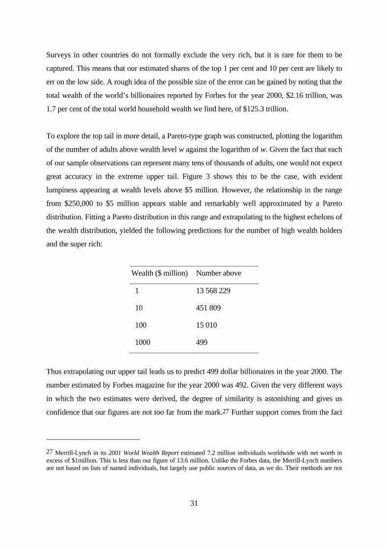
To explore the top tail in more detail, a Pareto-type graph was constructed, plotting the logarithm

of the number of adults above wealth level w against the logarithm of w. Given the fact that each

of our sample observations can represent many tens of thousands of adults, one would not expect

great accuracy in the extreme upper tail. Figure 3 shows this to be the case, with evident

lumpiness appearing at wealth levels above $5 million. However, the relationship in the range

from $250,000 to $5 million appears stable and remarkably well approximated by a Pareto

distribution. Fitting a Pareto distribution in this range and extrapolating to the highest echelons of

the wealth distribution, yielded the following predictions for the number of high wealth holders

and the super rich:

Wealth ($ million) Number above

1 13 568 229

10 451 809

100 15 010

1000 499

Thus extrapolating our upper tail leads us to predict 499 dollar billionaires in the year 2000. The

number estimated by Forbes magazine for the year 2000 was 492. Given the very different ways

in which the two estimates were derived, the degree of similarity is astonishing and gives us

confidence that our figures are not too far from the mark.27 Further support comes from the fact

27 Merrill-Lynch in its 2001 World Wealth Report estimated 7.2 million individuals worldwide with net worth in excess of $1million. This is less than our figure of 13.6 million. Unlike the Forbes data, the Merrill-Lynch numbers are not based on lists of named individuals, but largely use public sources of data, as we do. Their methods are not

32

that the Forbes data classifies 200 of the 492 dollar billionaires (i.e. 40.7 per cent) as US citizens,

a fraction that again conforms very closely with the data reported in Table 10b which gave a US

share of 37.4 per cent for the top 1 per cent and suggested that the share would rise further as

wealth increased.

6 Conclusion

This paper has provided a first estimate of the world distribution of household wealth. We have

seen that the distribution is highly concentrated — in fact much more concentrated than the

world distribution of income, or the distribution of wealth within all but a few of the world’s

countries. While a typical share of the top 10 per cent of wealth-holders within a country would

be about 50 per cent, and the median Gini around 0.7, we have estimated that for the world as a

whole the share of the top 10 per cent was 85 per cent in the year 2000 and the Gini equalled

0.892 using official exchange rates, Milanovic (2005) estimates that the world income Gini was

0.795 in 1998. While wealth (and income) concentration is somewhat less when the estimates are

done on a PPP basis, we have argued that the large share of wealth that is owned by people who

can readily travel and invest globally means that converting at official exchange rates is

preferable for many purposes when one is studying the distribution of wealth, rather than income

distribution or poverty.

Much of the data that is used here comes from household surveys. For the wealthiest country, the

US, which supplies 25 per cent of the world’s top 10 per cent of wealth-holders on an official

exchange rate basis (20 per cent using PPP), this is not a big problem. Sophisticated techniques

have been used by the Federal Reserve Board to make its triennial Survey of Consumer Finance

a reliable instrument. Less striking, but still effective steps have been taken in some of the other

wealthiest countries. While the super rich are not represented in these data, in terms of measuring

the overall degree of inequality we have seen that that is not a major deficiency. On the other

hand, surveys in the major developing countries appear to have a particular problem in capturing

well documented, so it is difficult to know why the number of millionaires is less than our estimate. But one likely explanation is that the Merrill Lynch wealth valuations exclude the family home and all consumer durables.

33

the upper tail. This means that while we have reasonable confidence in our estimates, there is a

non-negligible error bound that must be placed on them.

In evaluating the results obtained here it is important to keep in mind that the quality of the

estimates depends only in part on the accuracy of the distributional information that has been

assembled. It also depends on the accuracy of our estimates of mean household wealth in the

countries studied. Here we are on safer ground. For 33 countries, including all of the world’s

major OECD economies, we have data on the household sector’s financial balance sheet. And

for 18 of those countries we also have reasonable estimates of non-financial assets. These

estimates are often formed in conjunction with Flow of Funds numbers or the National Accounts.

There is a solid basis of good numbers from financial institutions and government statistical

agencies in these exercises.

Our study of wealth levels and composition across countries is not only important in providing a

key ingredient in estimating the world distribution of wealth. It is also of independent interest.

First, it gives us a picture of how wealth composition varies, not only with the stage of

development, but across countries at similar income levels due to institutional and traditional

differences, varying importance of public pensions, and other factors. Our empirical work has

shown how the importance of both financial assets and borrowing rises sharply with per capita

income and the development of financial markets. Conversely, we have seen how balance sheets

in poor countries are still dominated by land and other tangible assets. Secondly, we get a

snapshot of what Milanovic (2002, 2005) and others refer to as ‘international inequality’, that is

inequality between countries. On an official exchange rate basis per capita household wealth

ranged from about $1,100 for India to $144,000 for the United States in the year 2000. We have

also found that differences are large even for countries at a similar stage of development. Thus,

differences between countriesmake an important contribution to inequality in the world

distribution of household wealth. Even if the current level of wealth inequality within countries

proved to be enduring, one may hope for a significant reduction in world wealth inequality as

convergence takes place in wealth between nations.

Two caveats to conclusions about wealth inequality between countries (‘international

inequality’) are that the concentration is smaller when we measure on a PPP basis, and also less

on a per adult basis. Thus, for example, while the coefficient of variation for international

34

inequality is 2.141 on a per capita and official exchange rate basis, it is only 1.298 on a per adult

and PPP basis.

There is huge room for improvement in the study of household wealth from a global perspective.

Household balance sheets and wealth surveys need to be generated in more countries. These are

completely lacking in Latin America, and almost completely absent in Africa and most of Asia

as well. Financial development is a key aspect of economic growth and human development.

Without the relevant data it is impossible to see what progress is being made. Improvements in

data quality, particularly in survey data, must also occur. The task is far from hopeless, however,

and great strides have been taken in quite a few countries. The mere fact that regular wealth

surveys are conducted in the world’s two largest and most dynamic developing countries, China

and India, is very encouraging. As surveys are conducted in more developing and transition

countries, and as techniques for achieving greater accuracy, especially in the upper tail, are

applied in more countries, we will get a much better picture of the composition and distribution

of household wealth around the globe.

35

References

Ammermüller, A., Weber, A. and Westerheide P. (2005). Abschlussbericht zum Forschungsauftrag des Bundesministeriums für Gesundheit und Soziale Sicherung: Die Entwicklung und Verteilung des Vermögens privater Haulshalte unter besonderer Berücksichtigung de Produktivvermögens. Zentum für Europäische Wirtscaftsforschung.

Aron, Janine, John Muellbauer, and Johan Prinsloo (2006). ‘Estimating the Balance Sheet of the Personal Sector in an Emerging Market Country, South Africa 1970-2005’. Working paper, WIDER/UNU Project on Personal Assets From a Global Perspective.

Atkinson, Anthony B. and A.J. Harrison (1978). Distribution of Personal Wealth in Britain. Cambridge: Cambridge University Press.

Atkinson, Anthony B. (2006), ‘Concentration Among the Rich’, Working paper, WIDER/UNU Project on Personal Assets From a Global Perspective.

Australian Bureau of Statistics (2005). Household Income and Income Distribution Available from: http://www.abs.gov.au

Babeau, André and Teresa Sbano (2003). ‘Household Wealth in the National Accounts of Europe, the United States and Japan’. OECD Statistics Working Papers 2003/2.

Banco de Espana (2005)’Survey of Household Finances (EFF): Description, Methods and Preliminary Results’. Economic Bulletin January 2005.

Board of Governors of the Federal Reserve System (2003), Guide to Flow of Funds Accounts, Volume 1.

Bramall, C. (2001), ‘The Quality of China’s Household Income Surveys’, The China Quarterly 167: 689-705.

Brandolini, A., Cannari L., D’Alession G. and Faiella I. (2004). Household Wealth Distribution in Italy in the 1990s.Termi di discussione No 530. Rome: Bank of Italy.

Davies, James B. (1993). ‘The Distribution of Wealth in Canada’. Research in Economic Inequality 4: 159-180.

Davies, James B. and A.F. Shorrocks (2000). ‘The Distribution of Wealth’, Ch. 11 of Atkinson, Anthony B. and François Bourguignon, Handbook of Income Distribution Volume I, Amsterdam: Elsevier: 605-676.

Davies, James B. and Anthony Shorrocks (2005). ‘Wealth Holdings in Developing and Transition Countries’. Paper presented at a meeting of the Luxembourg Wealth Study, Perugia, January. Available

Dell, F., Piketty, T. and Saez, E. (2005). Income and Wealth Concentration in Switzerland over the 20th Century. Center for Economic Policy Research, Discussion Paper Series No. 5090. London: CEPR.

36

Goldsmith, Raymond W. (1985). Comparative National Balance Sheets, A Study of Twenty Countries, 1688-1978 Chicago: University of Chicago Press

Greene, William H. (1993), Econometric Analysis, Second Edition New York: Macmillan.

Headey, Bruce, Gary Marks and Mark Wooden (2005). ‘The Structure and Distribution of Household Wealth in Australia’. Australian Economic Review 38: 159-175.

Inland Revenue Statistics (2005). Distribution of Personal Wealth. Available from http://www.hmrc.gov.uk/stats/personal_wealth/menu.htm

International Monetary Fund (2005). Global Financial Stability Report, Market Developments and Issues. International Capital Markets Department. Available at http://www.imf.org/External/Pubs/FT/GFSR/2005/01/index.htm

Japan Statistics Bureau (2005). National Survey of Family Income and Expenditure 1999 [Internet]. Available from: http://www.stat.go.jp/english/data/zensho/index.htm

Kennickell, A. (2003). ‘A Rolling Tide: Changes in the Distribution of Wealth in the US, 1989-2001’. Levy Economics Institute of Bard College, Working Paper No. 393.

Kennickell, Arthur B. (2004). ‘The Good Shepherd: Sample Design and Control for Wealth Measurement in the Survey of Consumer Finances’, presented at the Perugia meeting of the Luxembourg Wealth Study, January 2005.

King, M.A. and J.I. Leape (1998). ‘Wealth and portfolio composition: theory and evidence’. Journal of Public Economics 69: 155-193.

Lane, Philip, and Gian Maria Milesi-Ferretti (2000). ‘The External Wealth of Nations, Measures of Foreign Assets and Liabilities For Industrial and Developing Countries’, working paper.

Leipziger, D.M., Dollar, D., Shorrocks, A.F. and Song, S.Y. (1992). The Distribution of Income and Wealth in Korea. Washington: The World Bank.

Mauro, Paulo, Nathan Sussman and Yishay Yafeh (forthcoming). Emerging Markets and Financial Globalization, Sovereign Bond Spreads in 1870-1913 and Today. Oxford: Oxford University Press.

Milanovic, Branko (2002). ‘True World Income Distribution, 1988 and 1993: First Calculation Based on Household Surveys Alone’, Economic Journal 112: 51-92.

Morissette, R. , Zhang, X. and Drolet, M. (2002). The Evolution of Wealth Inequality in Canada 1984-1999. No. 187, Feb 22. Ottawa: Statistics Canada.

National Sample Survey Organization. (2005). Household Assets and Liabilities in India (as on 30.06.2002): NSS 59th round (January-December 2003). Government of India: Ministry of Statistics and Programme Implementation.

Nolan , B. (1991). The Wealth of Irish Households: What Can We Learn from Survey Data? Dublin: Combat Poverty Agency.

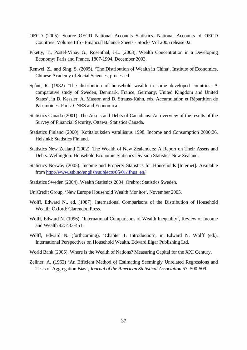
37

OECD (2005). Source OECD National Accounts Statistics. National Accounts of OECD Countries: Volume IIIb - Financial Balance Sheets - Stocks Vol 2005 release 02.

Piketty, T., Postel-Vinay G., Rosenthal, J-L. (2003). Wealth Concentration in a Developing Economy: Paris and France, 1807-1994. December 2003.

Renwei, Z., and Sing, S. (2005). ‘The Distribution of Wealth in China’. Institute of Economics, Chinese Academy of Social Sciences, processed.

Spånt, R. (1982) ‘The distribution of household wealth in some developed countries. A comparative study of Sweden, Denmark, France, Germany, United Kingdom and United States’, in D. Kessler, A. Masson and D. Strauss-Kahn, eds. Accumulation et Répartition de Patrimoines. Paris: CNRS and Economica.

Statistics Canada (2001). The Assets and Debts of Canadians: An overview of the results of the Survey of Financial Security. Ottawa: Statistics Canada.

Statistics Finland (2000). Kotitalouksien varallisuus 1998. Income and Consumption 2000:26. Helsinki: Statistics Finland.

Statistics New Zealand (2002). The Wealth of New Zealanders: A Report on Their Assets and Debts. Wellington: Household Economic Statistics Division Statistics New Zealand.

Statistics Norway (2005). Income and Property Statistics for Households [Internet]. Available from http://www.ssb.no/english/subjects/05/01/ifhus_en/

Statistics Sweden (2004). Wealth Statistics 2004. Örebro: Statistics Sweden.

UniCredit Group, ‘New Europe Household Wealth Monitor’, November 2005.

Wolff, Edward N., ed. (1987). International Comparisons of the Distribution of Household Wealth. Oxford: Clarendon Press.

Wolff, Edward N. (1996). ‘International Comparisons of Wealth Inequality’, Review of Income and Wealth 42: 433-451.

Wolff, Edward N. (forthcoming). ‘Chapter 1. Introduction’, in Edward N. Wolff (ed.), International Perspectives on Household Wealth, Edward Elgar Publishing Ltd.

World Bank (2005). Where is the Wealth of Nations? Measuring Capital for the XXI Century.

Zellner, A. (1962) ‘An Efficient Method of Estimating Seemingly Unrelated Regressions and Tests of Aggregation Bias’, Journal of the American Statistical Association 57: 500-509.

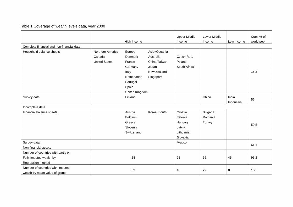
Table 1 Coverage of wealth levels data, year 2000

High income Upper Middle Income

Lower Middle Income Low Income

Cum. % of world pop.

Complete financial and non-financial data Household balance sheets Northern America Europe Asia+Oceania Canada Denmark Australia Czech Rep. United States France China,Taiwan Poland Germany Japan South Africa Italy New Zealand Netherlands Singapore Portugal Spain United Kingdom

15.3

Survey data Finland China India Indonesia

56

Incomplete data Financial balance sheets Austria Korea, South Croatia Bulgaria Belgium Estonia Romania Greece Hungary Turkey Slovenia Latvia Switzerland Lithuania Slovakia

59.5

Survey data: Mexico Non-financial assets

61.1

Number of countries with partly or Fully imputed wealth by Regression method

18 28 36 46 95.2

Number of countries with imputed wealth by mean value of group

33 16 22 8 100

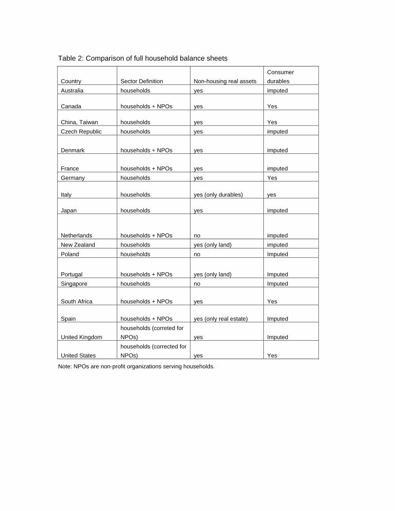
Table 2: Comparison of full household balance sheets

Country Sector Definition Non-housing real assets Consumer durables

Australia households yes imputed

Canada households + NPOs yes Yes

China, Taiwan households yes Yes Czech Republic households yes imputed

Denmark households + NPOs yes imputed

France households + NPOs yes imputed Germany households yes Yes

Italy households yes (only durables) yes

Japan households yes imputed

Netherlands households + NPOs no imputed New Zealand households yes (only land) imputed Poland households no Imputed

Portugal households + NPOs yes (only land) Imputed Singapore households no Imputed

South Africa households + NPOs yes Yes

Spain households + NPOs yes (only real estate) Imputed

United Kingdom households (correted for NPOs) yes Imputed

United States households (corrected for NPOs) yes Yes

Note: NPOs are non-profit organizations serving households.

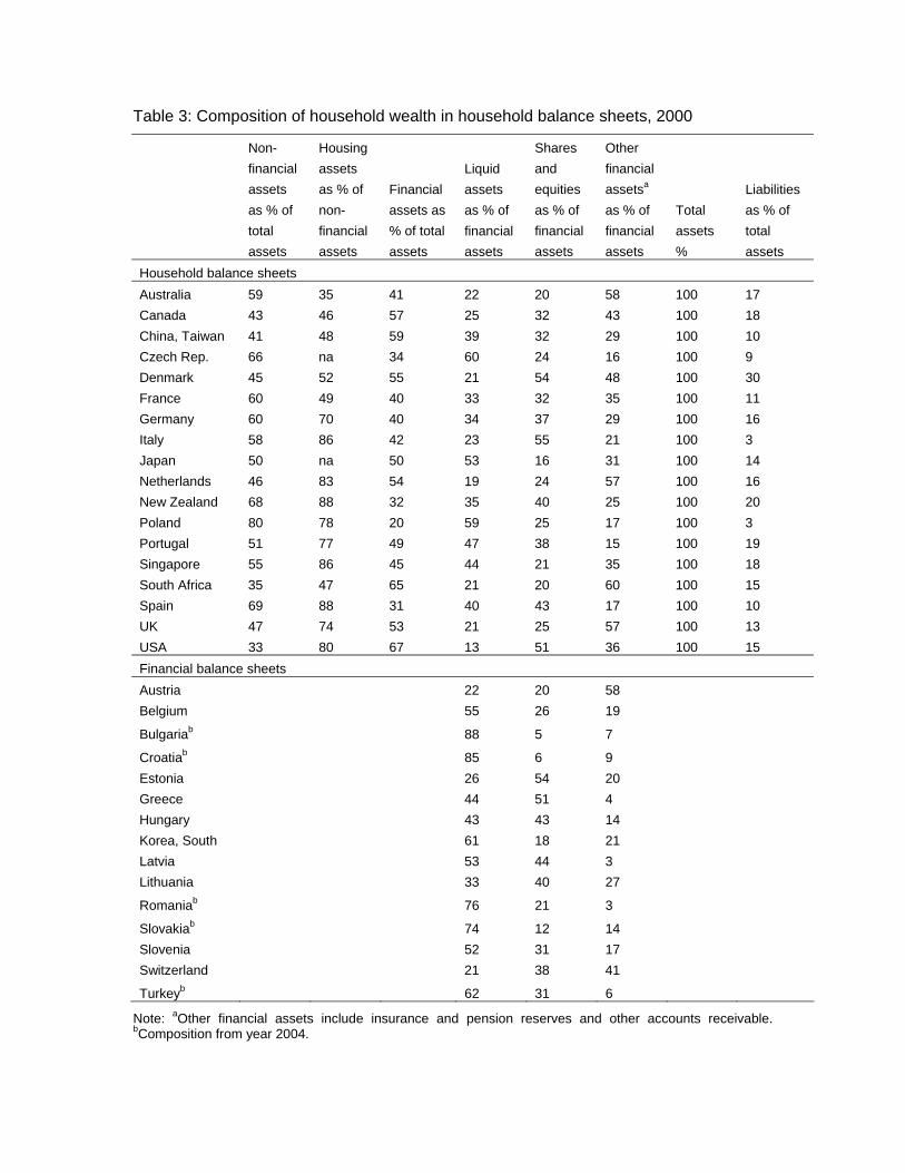
Table 3: Composition of household wealth in household balance sheets, 2000

Non-financial assets as % of total assets

Housing assets as % of non-financial assets

Financial assets as % of total assets

Liquid assets as % of financial assets

Shares and equities as % of financial assets

Other financial assetsa as % of financial assets

Total assets %

Liabilities as % of total assets

Household balance sheets Australia 59 35 41 22 20 58 100 17 Canada 43 46 57 25 32 43 100 18 China, Taiwan 41 48 59 39 32 29 100 10 Czech Rep. 66 na 34 60 24 16 100 9 Denmark 45 52 55 21 54 48 100 30 France 60 49 40 33 32 35 100 11 Germany 60 70 40 34 37 29 100 16 Italy 58 86 42 23 55 21 100 3 Japan 50 na 50 53 16 31 100 14 Netherlands 46 83 54 19 24 57 100 16 New Zealand 68 88 32 35 40 25 100 20 Poland 80 78 20 59 25 17 100 3 Portugal 51 77 49 47 38 15 100 19 Singapore 55 86 45 44 21 35 100 18 South Africa 35 47 65 21 20 60 100 15 Spain 69 88 31 40 43 17 100 10 UK 47 74 53 21 25 57 100 13 USA 33 80 67 13 51 36 100 15 Financial balance sheets Austria 22 20 58 Belgium 55 26 19

Bulgariab 88 5 7

Croatiab 85 6 9 Estonia 26 54 20 Greece 44 51 4 Hungary 43 43 14 Korea, South 61 18 21 Latvia 53 44 3 Lithuania 33 40 27

Romaniab 76 21 3

Slovakiab 74 12 14 Slovenia 52 31 17 Switzerland 21 38 41

Turkeyb 62 31 6

Note: aOther financial assets include insurance and pension reserves and other accounts receivable. bComposition from year 2004.

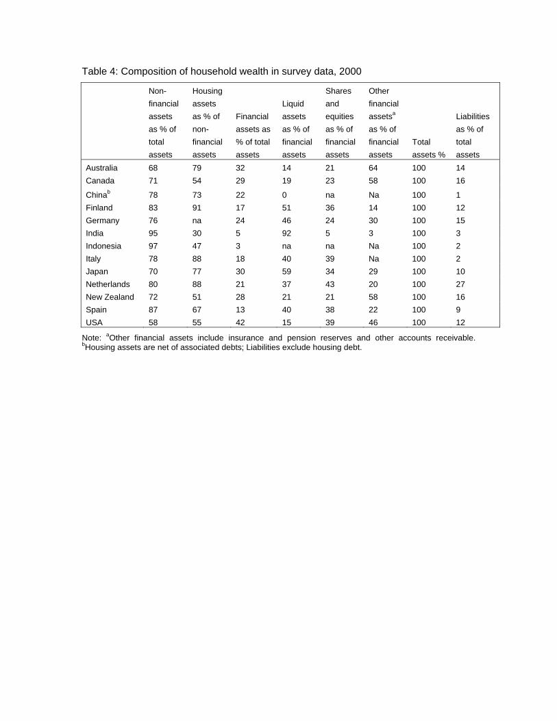
Table 4: Composition of household wealth in survey data, 2000

Non-financial assets as % of total assets

Housing assets as % of non-financial assets

Financial assets as % of total assets

Liquid assets as % of financial assets

Shares and equities as % of financial assets

Other financial assetsa as % of financial assets

Total assets %

Liabilities as % of total assets

Australia 68 79 32 14 21 64 100 14 Canada 71 54 29 19 23 58 100 16

Chinab 78 73 22 0 na Na 100 1 Finland 83 91 17 51 36 14 100 12 Germany 76 na 24 46 24 30 100 15 India 95 30 5 92 5 3 100 3 Indonesia 97 47 3 na na Na 100 2 Italy 78 88 18 40 39 Na 100 2 Japan 70 77 30 59 34 29 100 10 Netherlands 80 88 21 37 43 20 100 27 New Zealand 72 51 28 21 21 58 100 16 Spain 87 67 13 40 38 22 100 9 USA 58 55 42 15 39 46 100 12

Note: aOther financial assets include insurance and pension reserves and other accounts receivable. bHousing assets are net of associated debts; Liabilities exclude housing debt.

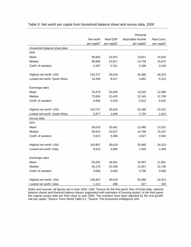
Table 5: Net worth per capita from household balance sheet and survey data, 2000

Net worth

per capitaaReal GDP per capitab

Personal disposable income

per capitacReal Cons. per capitab

Household balance sheet data PPP Mean 85,682 22,921 13,811 14,342 Median 90,906 23,917 14,739 15,672 Coeff. of variation 0.427 0.311 0.326 0.319 Highest net worth: USA 143,727 35,619 25,480 24,313 Lowest net worth: South Africa 16,266 8,017 4,691 5,210 Exchange rates Mean 76,479 20,006 12,020 12,486 Median 73,654 21,425 12,145 12,708 Coeff. of variation 0.594 0.519 0.522 0.525 Highest net worth: USA 143,727 35,619 25,480 24,313 Lowest net worth: South Africa 5,977 2,946 1,724 1,914 Survey data PPP Mean 59,010 20,461 12,485 13,231 Median 60,614 23,917 12,798 15,197 Coeff. of variation 0.672 0.496 0.527 0.504 Highest net worth: USA 143,857 35,619 25,480 24,313 Lowest net worth: India 6,513 2,684 1,916 1,406 Exchange rates Mean 53,251 18,031 10,947 11,661 Median 45,176 20,338 11,557 12,708 Coeff. of variation 0.836 0.663 0.700 0.658 Highest net worth: USA 143,857 35,619 25,480 24,313 Lowest net worth: India 1,112 458 327 240

Notes and sources: all figures are in year 2000, US$. aSource for the first panel: flow of funds data, national balance sheets and financial balance sheets augmented with estimates of housing assets. In the third panel the original survey data are from close to year 2000. The numbers have been adjusted by the real growth rate per capita. bSource: Penn World Table 6.1. cSource: The Economist Intelligence Unit.

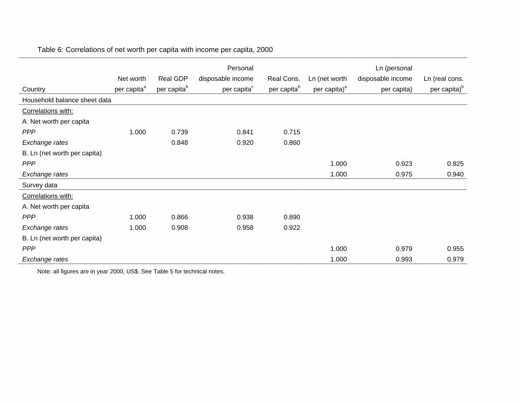
Table 6: Correlations of net worth per capita with income per capita, 2000

Country Net worth

per capitaa

Real GDP per capitab

Personal disposable income

per capitac

Real Cons. per capitab

Ln (net worth per capita)a

Ln (personal disposable income

per capita)Ln (real cons.

per capita)b

Household balance sheet data Correlations with: A. Net worth per capita PPP 1.000 0.739 0.841 0.715 Exchange rates 0.848 0.920 0.860 B. Ln (net worth per capita) PPP 1.000 0.923 0.825Exchange rates 1.000 0.975 0.940Survey data Correlations with: A. Net worth per capita PPP 1.000 0.866 0.938 0.890 Exchange rates 1.000 0.908 0.958 0.922 B. Ln (net worth per capita) PPP 1.000 0.979 0.955Exchange rates 1.000 0.993 0.979

Note: all figures are in year 2000, US$. See Table 5 for technical notes.

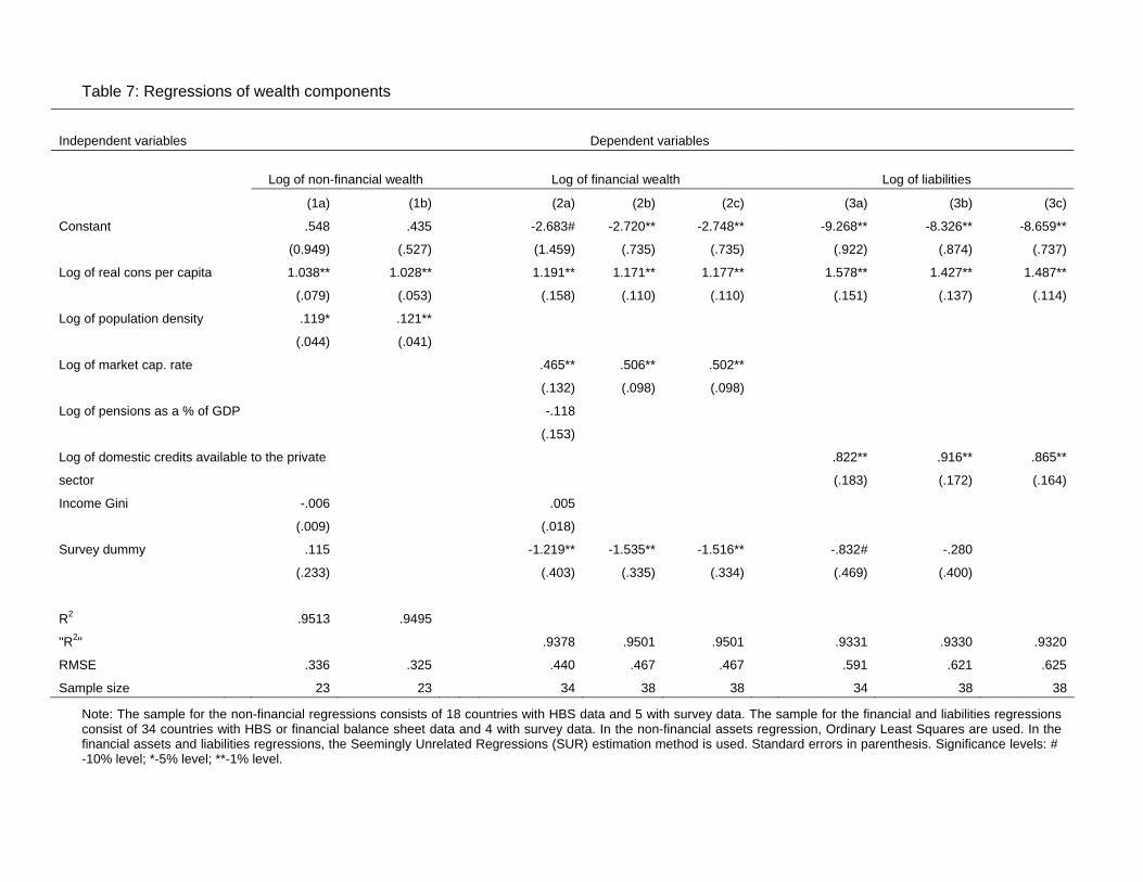
Table 7: Regressions of wealth components

Independent variables Dependent variables

Log of non-financial wealth Log of financial wealth Log of liabilities

(1a) (1b) (2a) (2b) (2c) (3a) (3b) (3c)

Constant .548 .435 -2.683# -2.720** -2.748** -9.268** -8.326** -8.659**

(0.949) (.527) (1.459) (.735) (.735) (.922) (.874) (.737)

Log of real cons per capita 1.038** 1.028** 1.191** 1.171** 1.177** 1.578** 1.427** 1.487**

(.079) (.053) (.158) (.110) (.110) (.151) (.137) (.114)

Log of population density .119* .121**

(.044) (.041)

Log of market cap. rate .465** .506** .502**

(.132) (.098) (.098)

Log of pensions as a % of GDP -.118

(.153)

.822** .916** .865** Log of domestic credits available to the private

sector (.183) (.172) (.164)

Income Gini -.006 .005

(.009) (.018)

Survey dummy .115 -1.219** -1.535** -1.516** -.832# -.280

(.233) (.403) (.335) (.334) (.469) (.400)

R2 .9513 .9495

"R2" .9378 .9501 .9501 .9331 .9330 .9320

RMSE .336 .325 .440 .467 .467 .591 .621 .625

Sample size 23 23 34 38 38 34 38 38

Note: The sample for the non-financial regressions consists of 18 countries with HBS data and 5 with survey data. The sample for the financial and liabilities regressions consist of 34 countries with HBS or financial balance sheet data and 4 with survey data. In the non-financial assets regression, Ordinary Least Squares are used. In the financial assets and liabilities regressions, the Seemingly Unrelated Regressions (SUR) estimation method is used. Standard errors in parenthesis. Significance levels: # -10% level; *-5% level; **-1% level.

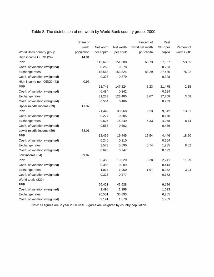
Table 8: The distribution of net worth by World Bank country group, 2000

World Bank country group

Share of world

population Net worth per capita

Net worth per adult

Percent of world net worth

per capita

Real GDP per

capita Percent of world GDP

High income OECD (24) 14.81 PPP 113,675 151,308 63.73 27,367 53.55 Coeff. of variation (weighted) 0.260 0.278 0.233 Exchange rates 115,565 153,824 83.29 27,430 76.92 Coeff. of variation (weighted) 0.377 0.379 0.328 High income non-OECD (43) 0.93 PPP 91,748 147,524 3.23 21,475 2.35 Coeff. of variation (weighted) 0.484 0.342 0.184 Exchange rates 81,233 123,485 3.67 17,708 3.08 Coeff. of variation (weighted) 0.534 0.406 0.233 Upper middle income (39) 11.37 PPP 21,442 33,968 9.23 9,342 13.91 Coeff. of variation (weighted) 0.277 0.285 0.170 Exchange rates 9,626 15,249 5.33 4,058 8.74 Coeff. of variation (weighted) 0.553 0.602 0.456 Lower middle income (59) 33.01 PPP 12,436 19,445 15.54 4,446 18.90 Coeff. of variation (weighted) 0.240 0.310 0.264 Exchange rates 3,573 5,590 5.74 1,285 8.02 Coeff. of variation (weighted) 0.626 0.747 0.692 Low income (64) 39.87 PPP 5,485 10,520 8.28 2,241 11.29 Coeff. of variation (weighted) 0.385 0.309 0.413 Exchange rates 1,017 1,950 1.97 0.372 3.24 Coeff. of variation (weighted) 0.328 0.277 0.372 World totals (229) PPP 26,421 43,628 9,186 Coeff. of variation (weighted) 1.498 1.298 1.093 Exchange rates 20,551 33,893 6,205 Coeff. of variation (weighted) 2.141 1.878 1.769

Note: all figures are in year 2000 US$. Figures are weighted by country population.

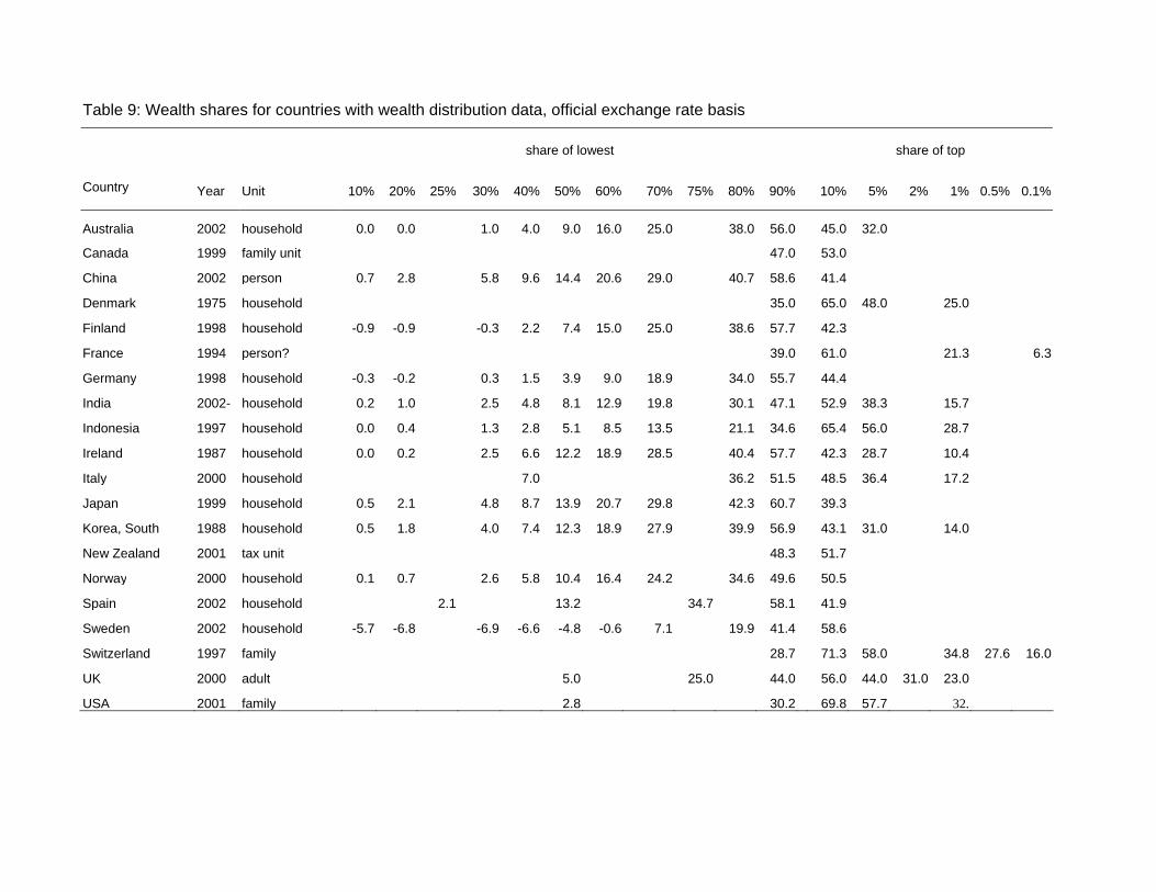
Table 9: Wealth shares for countries with wealth distribution data, official exchange rate basis

share of lowest share of top

Country Year Unit 10% 20% 25% 30% 40% 50% 60% 70% 75% 80% 90% 10% 5% 2% 1% 0.5% 0.1%

Australia 2002 household 0.0 0.0 1.0 4.0 9.0 16.0 25.0 38.0 56.0 45.0 32.0

Canada 1999 family unit 47.0 53.0

China 2002 person 0.7 2.8 5.8 9.6 14.4 20.6 29.0 40.7 58.6 41.4

Denmark 1975 household 35.0 65.0 48.0 25.0

Finland 1998 household -0.9 -0.9 -0.3 2.2 7.4 15.0 25.0 38.6 57.7 42.3

France 1994 person? 39.0 61.0 21.3 6.3

Germany 1998 household -0.3 -0.2 0.3 1.5 3.9 9.0 18.9 34.0 55.7 44.4

India 2002- household 0.2 1.0 2.5 4.8 8.1 12.9 19.8 30.1 47.1 52.9 38.3 15.7

Indonesia 1997 household 0.0 0.4 1.3 2.8 5.1 8.5 13.5 21.1 34.6 65.4 56.0 28.7

Ireland 1987 household 0.0 0.2 2.5 6.6 12.2 18.9 28.5 40.4 57.7 42.3 28.7 10.4

Italy 2000 household 7.0 36.2 51.5 48.5 36.4 17.2

Japan 1999 household 0.5 2.1 4.8 8.7 13.9 20.7 29.8 42.3 60.7 39.3

Korea, South 1988 household 0.5 1.8 4.0 7.4 12.3 18.9 27.9 39.9 56.9 43.1 31.0 14.0

New Zealand 2001 tax unit 48.3 51.7

Norway 2000 household 0.1 0.7 2.6 5.8 10.4 16.4 24.2 34.6 49.6 50.5

Spain 2002 household 2.1 13.2 34.7 58.1 41.9

Sweden 2002 household -5.7 -6.8 -6.9 -6.6 -4.8 -0.6 7.1 19.9 41.4 58.6

Switzerland 1997 family 28.7 71.3 58.0 34.8 27.6 16.0

UK 2000 adult 5.0 25.0 44.0 56.0 44.0 31.0 23.0

USA 2001 family 2.8 30.2 69.8 57.7 32.

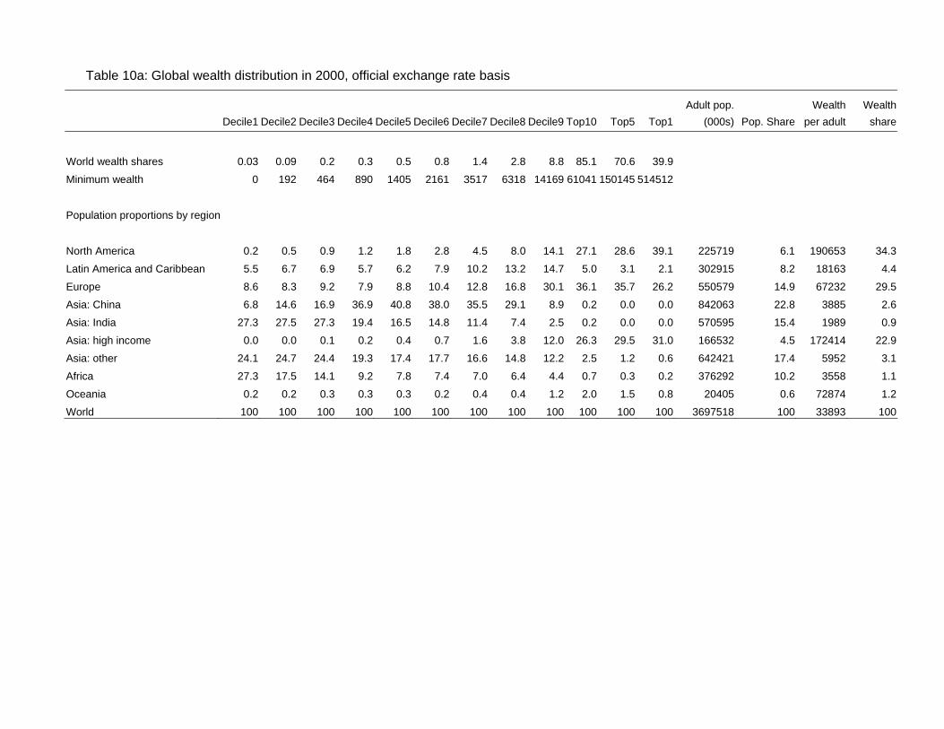
Table 10a: Global wealth distribution in 2000, official exchange rate basis

Decile1 Decile2 Decile3 Decile4 Decile5 Decile6 Decile7 Decile8 Decile9 Top10 Top5 Top1Adult pop.

(000s) Pop. ShareWealth

per adultWealth

share

World wealth shares 0.03 0.09 0.2 0.3 0.5 0.8 1.4 2.8 8.8 85.1 70.6 39.9

Minimum wealth 0 192 464 890 1405 2161 3517 6318 14169 61041 150145 514512

Population proportions by region

North America 0.2 0.5 0.9 1.2 1.8 2.8 4.5 8.0 14.1 27.1 28.6 39.1 225719 6.1 190653 34.3

Latin America and Caribbean 5.5 6.7 6.9 5.7 6.2 7.9 10.2 13.2 14.7 5.0 3.1 2.1 302915 8.2 18163 4.4

Europe 8.6 8.3 9.2 7.9 8.8 10.4 12.8 16.8 30.1 36.1 35.7 26.2 550579 14.9 67232 29.5

Asia: China 6.8 14.6 16.9 36.9 40.8 38.0 35.5 29.1 8.9 0.2 0.0 0.0 842063 22.8 3885 2.6

Asia: India 27.3 27.5 27.3 19.4 16.5 14.8 11.4 7.4 2.5 0.2 0.0 0.0 570595 15.4 1989 0.9

Asia: high income 0.0 0.0 0.1 0.2 0.4 0.7 1.6 3.8 12.0 26.3 29.5 31.0 166532 4.5 172414 22.9

Asia: other 24.1 24.7 24.4 19.3 17.4 17.7 16.6 14.8 12.2 2.5 1.2 0.6 642421 17.4 5952 3.1

Africa 27.3 17.5 14.1 9.2 7.8 7.4 7.0 6.4 4.4 0.7 0.3 0.2 376292 10.2 3558 1.1

Oceania 0.2 0.2 0.3 0.3 0.3 0.2 0.4 0.4 1.2 2.0 1.5 0.8 20405 0.6 72874 1.2

World 100 100 100 100 100 100 100 100 100 100 100 100 3697518 100 33893 100

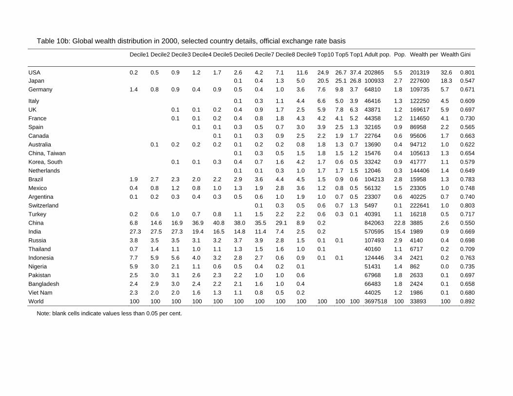
Table 10b: Global wealth distribution in 2000, selected country details, official exchange rate basis

Decile1 Decile2 Decile3 Decile4 Decile5 Decile6 Decile7 Decile8 Decile9 Top10 Top5 Top1 Adult pop. Pop. Wealth per Wealth Gini

USA 0.2 0.5 0.9 1.2 1.7 2.6 4.2 7.1 11.6 24.9 26.7 37.4 202865 5.5 201319 32.6 0.801Japan 0.1 0.4 1.3 5.0 20.5 25.1 26.8 100933 2.7 227600 18.3 0.547Germany 1.4 0.8 0.9 0.4 0.9 0.5 0.4 1.0 3.6 7.6 9.8 3.7 64810 1.8 109735 5.7 0.671

Italy 0.1 0.3 1.1 4.4 6.6 5.0 3.9 46416 1.3 122250 4.5 0.609UK 0.1 0.1 0.2 0.4 0.9 1.7 2.5 5.9 7.8 6.3 43871 1.2 169617 5.9 0.697France 0.1 0.1 0.2 0.4 0.8 1.8 4.3 4.2 4.1 5.2 44358 1.2 114650 4.1 0.730Spain 0.1 0.1 0.3 0.5 0.7 3.0 3.9 2.5 1.3 32165 0.9 86958 2.2 0.565Canada 0.1 0.1 0.3 0.9 2.5 2.2 1.9 1.7 22764 0.6 95606 1.7 0.663Australia 0.1 0.2 0.2 0.2 0.1 0.2 0.2 0.8 1.8 1.3 0.7 13690 0.4 94712 1.0 0.622China, Taiwan 0.1 0.3 0.5 1.5 1.8 1.5 1.2 15476 0.4 105613 1.3 0.654Korea, South 0.1 0.1 0.3 0.4 0.7 1.6 4.2 1.7 0.6 0.5 33242 0.9 41777 1.1 0.579Netherlands 0.1 0.1 0.3 1.0 1.7 1.7 1.5 12046 0.3 144406 1.4 0.649Brazil 1.9 2.7 2.3 2.0 2.2 2.9 3.6 4.4 4.5 1.5 0.9 0.6 104213 2.8 15958 1.3 0.783Mexico 0.4 0.8 1.2 0.8 1.0 1.3 1.9 2.8 3.6 1.2 0.8 0.5 56132 1.5 23305 1.0 0.748Argentina 0.1 0.2 0.3 0.4 0.3 0.5 0.6 1.0 1.9 1.0 0.7 0.5 23307 0.6 40225 0.7 0.740Switzerland 0.1 0.3 0.5 0.6 0.7 1.3 5497 0.1 222641 1.0 0.803Turkey 0.2 0.6 1.0 0.7 0.8 1.1 1.5 2.2 2.2 0.6 0.3 0.1 40391 1.1 16218 0.5 0.717China 6.8 14.6 16.9 36.9 40.8 38.0 35.5 29.1 8.9 0.2 842063 22.8 3885 2.6 0.550India 27.3 27.5 27.3 19.4 16.5 14.8 11.4 7.4 2.5 0.2 570595 15.4 1989 0.9 0.669Russia 3.8 3.5 3.5 3.1 3.2 3.7 3.9 2.8 1.5 0.1 0.1 107493 2.9 4140 0.4 0.698Thailand 0.7 1.4 1.1 1.0 1.1 1.3 1.5 1.6 1.0 0.1 40160 1.1 6717 0.2 0.709Indonesia 7.7 5.9 5.6 4.0 3.2 2.8 2.7 0.6 0.9 0.1 0.1 124446 3.4 2421 0.2 0.763Nigeria 5.9 3.0 2.1 1.1 0.6 0.5 0.4 0.2 0.1 51431 1.4 862 0.0 0.735Pakistan 2.5 3.0 3.1 2.6 2.3 2.2 1.0 1.0 0.6 67968 1.8 2633 0.1 0.697Bangladesh 2.4 2.9 3.0 2.4 2.2 2.1 1.6 1.0 0.4 66483 1.8 2424 0.1 0.658Viet Nam 2.3 2.0 2.0 1.6 1.3 1.1 0.8 0.5 0.2 44025 1.2 1986 0.1 0.680World 100 100 100 100 100 100 100 100 100 100 100 100 3697518 100 33893 100 0.892

Note: blank cells indicate values less than 0.05 per cent.

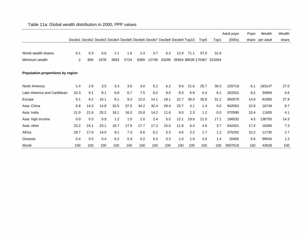
Table 11a: Global wealth distribution in 2000, PPP values

Decile1 Decile2 Decile3 Decile4 Decile5 Decile6 Decile7 Decile8 Decile9 Top10 Top5 Top1

Adult popn

(000s)

Popn

share

Wealth

per adult

Wealth

share

World wealth shares 0.1 0.3 0.6 1.1 1.6 2.4 3.7 6.2 12.9 71.1 57.0 31.6

Minimum wealth 2 826 1978 3693 5724 8399 12749 20299 35954 88035 170467 523264

Population proportions by region

North America 1.4 2.6 3.5 3.3 3.5 4.0 5.2 6.2 9.6 21.6 25.7 39.3 225719 6.1 193147 27.0

Latin America and Caribbean 10.3 9.1 8.1 6.8 6.7 7.5 8.2 9.0 9.3 6.9 6.4 6.1 302915 8.2 34956 6.6

Europe 9.1 9.2 10.1 9.1 9.3 12.0 14.1 18.1 22.7 35.0 35.8 31.2 550579 14.9 81890 27.9

Asia: China 6.8 14.3 14.8 33.5 37.5 34.2 32.4 29.4 20.7 4.1 1.4 0.0 842063 22.8 16749 8.7

Asia: India 21.0 21.9 25.2 18.1 16.3 15.8 14.2 11.6 8.0 2.3 1.2 0.0 570595 15.4 11655 4.1

Asia: high income 0.0 0.3 0.9 1.2 1.5 2.0 2.4 5.0 12.1 19.6 21.0 17.1 166532 4.5 138750 14.3

Asia: other 22.2 24.1 23.1 18.7 17.5 17.7 17.2 15.0 11.9 6.4 4.9 3.7 642421 17.4 18266 7.3

Africa 28.7 17.9 14.0 9.1 7.3 6.6 6.1 5.3 4.6 2.2 1.7 1.2 376292 10.2 11730 2.7

Oceania 0.4 0.5 0.4 0.2 0.3 0.2 0.2 0.3 1.0 1.9 2.0 1.4 20405 0.6 99634 1.3

World 100 100 100 100 100 100 100 100 100 100 100 100 3697519 100 43628 100

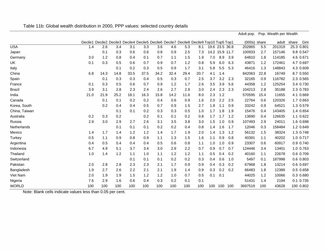
Table 11b: Global wealth distribution in 2000, PPP values: selected country details

Decile1 Decile2 Decile3 Decile4 Decile5 Decile6 Decile7

Decile8 Decile9 Top10 Top5 Top1

Adult pop.

(000s)

Pop.

share

Wealth per

adult

Wealth

share

Gini USA 1.4 2.6 3.4 3.1 3.3 3.6 4.6 5.3 8.1 19.6 23.5 36.8 202865 5.5 201319 25.3 0.801 Japan 0.1 0.3 0.6 0.6 0.8 0.9 2.5 7.3 14.2 15.9 11.7 100933 2.7 157146 9.8 0.547 Germany 3.0 1.2 0.8 0.4 0.1 0.7 1.1 1.5 1.9 7.0 8.9 3.9 64810 1.8 114185 4.6 0.671 UK 0.1 0.3 0.5 0.6 0.7 0.9 0.7 1.2 0.8 5.9 6.0 6.3 43871 1.2 172461 4.7 0.697 Italy 0.1 0.2 0.3 0.5 0.9 1.7 3.1 5.8 5.5 5.3 46416 1.3 148843 4.3 0.609 China 6.8 14.3 14.8 33.5 37.5 34.2 32.4 29.4 20.7 4.1 1.4 842063 22.8 16749 8.7 0.550 Spain 0.1 0.3 0.3 0.4 0.5 0.3 0.7 2.5 3.7 3.2 2.3 32165 0.9 116782 2.3 0.565 France 0.1 0.3 0.5 0.6 0.7 0.9 1.2 1.7 2.6 3.5 3.9 5.6 44358 1.2 125254 3.4 0.730 Brazil 3.9 3.1 2.8 2.3 2.4 2.6 2.7 2.9 3.0 2.4 2.3 2.3 104213 2.8 35188 2.3 0.783 India 21.0 21.9 25.2 18.1 16.3 15.8 14.2 11.6 8.0 2.3 1.2 570595 15.4 11655 4.1 0.669 Canada 0.1 0.1 0.2 0.2 0.4 0.6 0.9 1.6 2.0 2.2 2.5 22764 0.6 120326 1.7 0.663 Korea, South 0.2 0.4 0.4 0.5 0.7 0.9 1.5 2.7 1.8 1.1 0.9 33242 0.9 64521 1.3 0.579 China, Taiwan 0.1 0.1 0.2 0.3 0.3 0.5 1.0 1.7 1.8 1.9 15476 0.4 143405 1.4 0.654 Australia 0.2 0.3 0.2 0.2 0.1 0.1 0.2 0.8 1.7 1.7 1.2 13690 0.4 126635 1.1 0.622 Russia 2.9 3.0 2.9 2.7 2.6 3.1 3.5 3.8 3.0 1.5 1.0 0.9 107493 2.9 24011 1.6 0.698 Netherlands 0.1 0.1 0.1 0.2 0.2 0.4 0.8 1.4 1.6 1.7 12046 0.3 158484 1.2 0.649 Mexico 1.4 1.7 1.4 1.2 1.2 1.4 1.7 1.9 2.0 1.4 1.3 1.2 56132 1.5 38324 1.3 0.748 Turkey 0.5 1.1 0.9 0.8 0.9 1.1 1.3 1.5 1.6 1.1 0.9 0.8 40391 1.1 40202 1.0 0.717 Argentina 0.4 0.5 0.4 0.4 0.4 0.5 0.6 0.8 1.1 1.0 1.0 0.9 23307 0.6 60917 0.9 0.740 Indonesia 6.7 4.9 5.1 3.7 3.4 3.0 2.9 2.2 0.7 0.9 0.7 0.7 124446 3.4 13401 1.0 0.763 Thailand 1.0 1.4 1.2 1.1 1.0 1.1 1.2 1.2 1.1 0.5 0.4 0.2 40160 1.1 22678 0.6 0.709 Switzerland 0.1 0.1 0.1 0.2 0.2 0.3 0.4 0.6 1.0 5497 0.1 187998 0.6 0.803 Pakistan 2.0 2.8 2.8 2.3 2.3 2.1 1.7 0.9 0.9 0.4 0.3 0.2 67968 1.8 13214 0.6 0.697 Bangladesh 1.9 2.7 2.6 2.2 2.1 2.1 1.9 1.4 0.9 0.3 0.2 0.2 66483 1.8 12389 0.5 0.658 Viet Nam 2.0 1.9 1.9 1.5 1.2 1.2 1.0 0.7 0.5 0.1 0.1 44025 1.2 10066 0.3 0.680 Nigeria 7.6 2.9 1.6 0.6 0.4 0.3 0.2 0.1 0.1 51431 1.4 2194 0.1 0.735 WORLD 100 100 100 100 100 100 100 100 100 100 100 100 3697519 100 43628 100 0.802

Note: Blank cells indicate values less than 0.05 per cent.

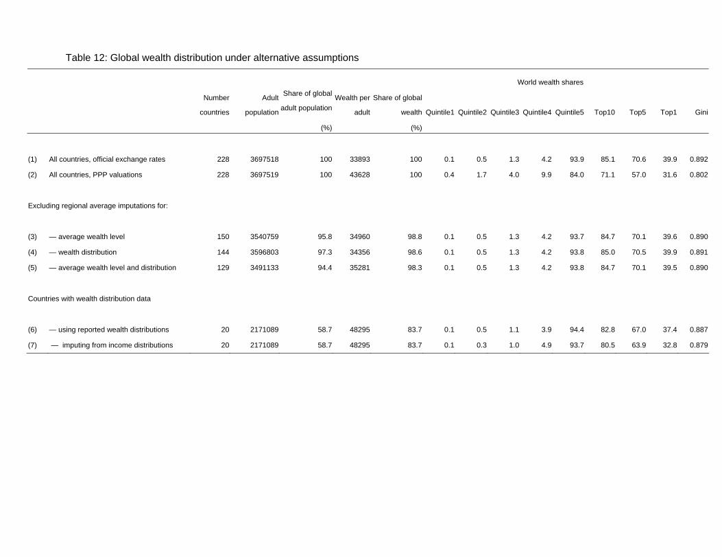
Table 12: Global wealth distribution under alternative assumptions

World wealth shares

Number

countries

Adult

population

Share of global

adult populationWealth per

adult

Share of global

wealth Quintile1 Quintile2 Quintile3 Quintile4 Quintile5 Top10 Top5 Top1 Gini

(%) (%)

(1) All countries, official exchange rates 228 3697518 100 33893 100 0.1 0.5 1.3 4.2 93.9 85.1 70.6 39.9 0.892

(2) All countries, PPP valuations 228 3697519 100 43628 100 0.4 1.7 4.0 9.9 84.0 71.1 57.0 31.6 0.802

Excluding regional average imputations for:

(3) — average wealth level 150 3540759 95.8 34960 98.8 0.1 0.5 1.3 4.2 93.7 84.7 70.1 39.6 0.890

(4) — wealth distribution 144 3596803 97.3 34356 98.6 0.1 0.5 1.3 4.2 93.8 85.0 70.5 39.9 0.891

(5) — average wealth level and distribution 129 3491133 94.4 35281 98.3 0.1 0.5 1.3 4.2 93.8 84.7 70.1 39.5 0.890

Countries with wealth distribution data

(6) — using reported wealth distributions 20 2171089 58.7 48295 83.7 0.1 0.5 1.1 3.9 94.4 82.8 67.0 37.4 0.887

(7) — imputing from income distributions 20 2171089 58.7 48295 83.7 0.1 0.3 1.0 4.9 93.7 80.5 63.9 32.8 0.879

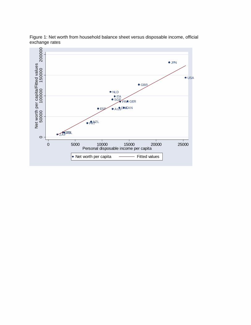
Figure 1: Net worth from household balance sheet versus disposable income, official exchange rates

AUS CAN

CZE

DNK

FRA GERITA

JPN

NLD

NZL

POL

PRT

SGP

ZAF

ESP

GBR

USA

050

000

1000

0015

0000

2000

00N

et w

orth

per

cap

ita/F

itted

val

ues

0 5000 10000 15000 20000 25000Personal disposable income per capita

Net worth per capita Fitted values

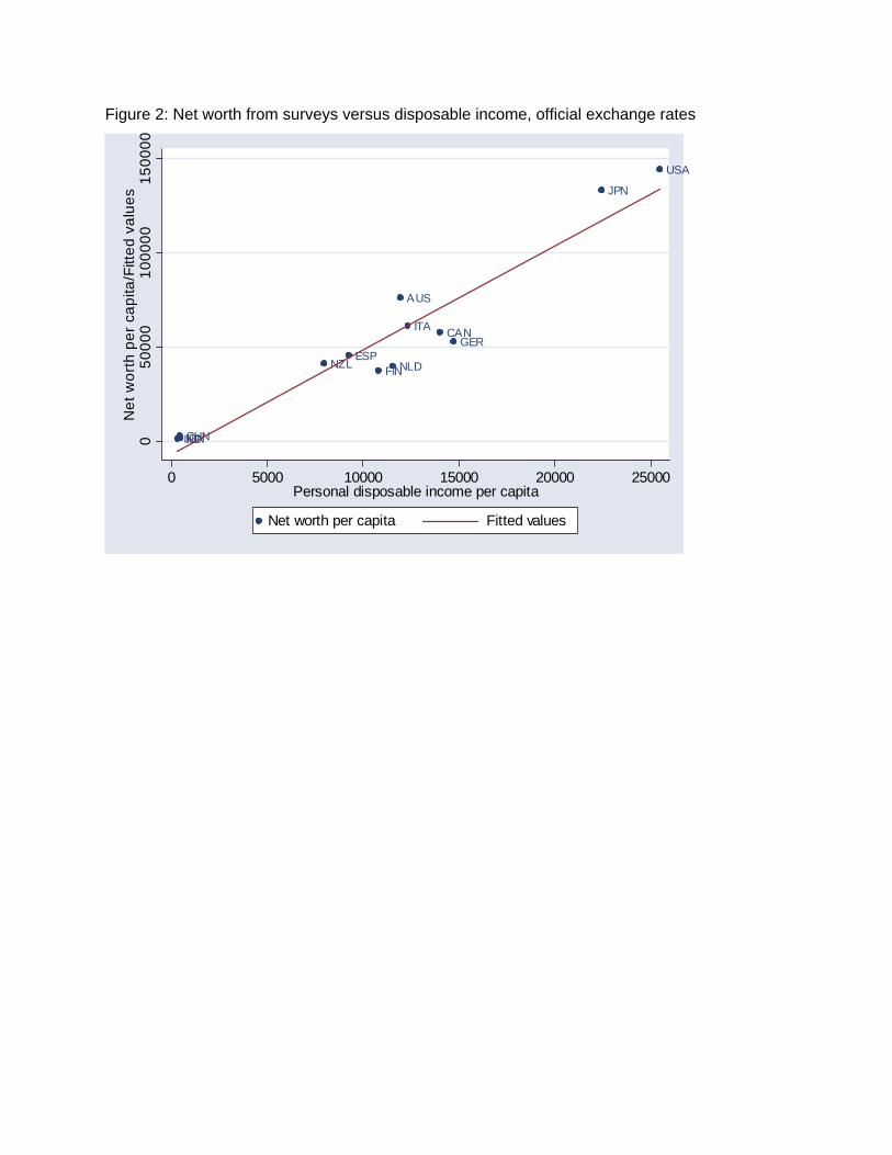
Figure 2: Net worth from surveys versus disposable income, official exchange rates

AUS

CAN

CHN

FIN

GER

INDIDN

ITA

JPN

NLDNZLESP

USA

050

000

1000

0015

0000

Net

wor

th p

er c

apita

/Fitt

ed v

alue

s

0 5000 10000 15000 20000 25000Personal disposable income per capita

Net worth per capita Fitted values

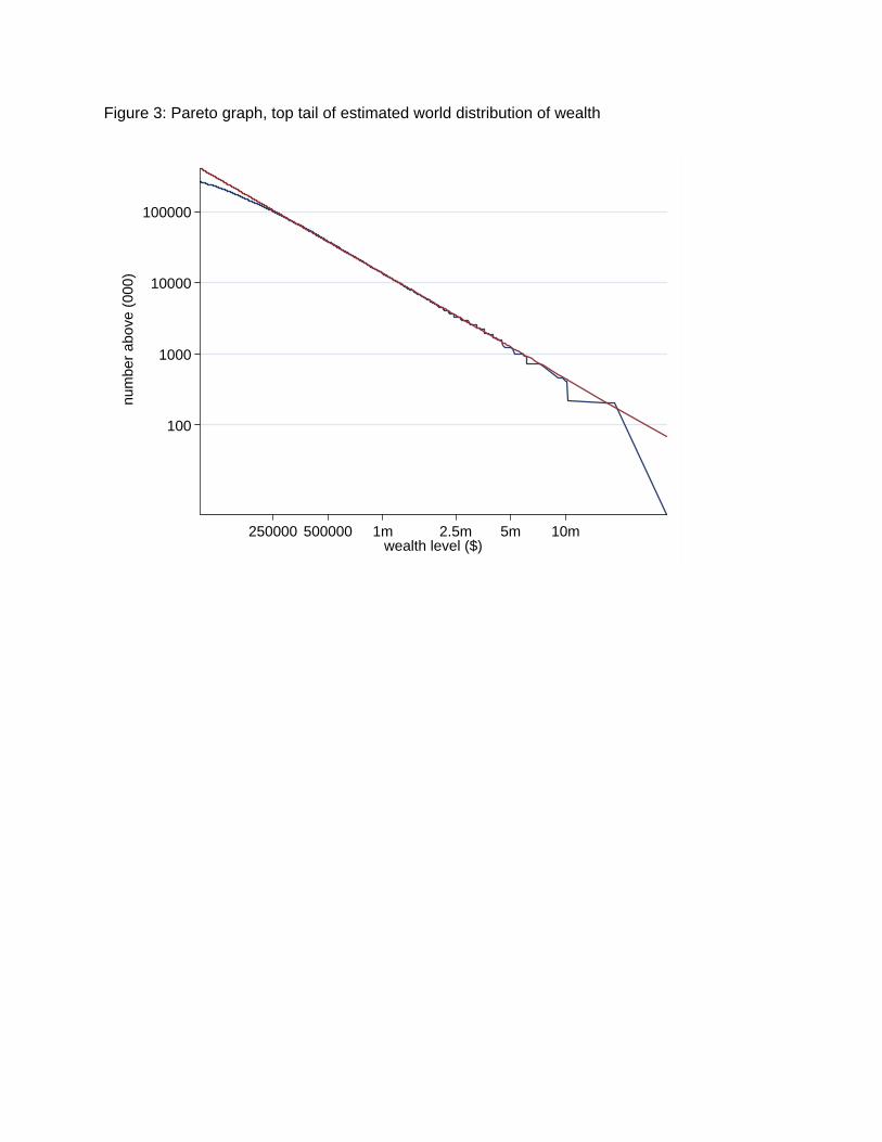
Figure 3: Pareto graph, top tail of estimated world distribution of wealth

10000

1000

100000

num

ber a

bove

(000

)

100

250000 500000 1m 2.5m 5m 10mwealth level ($)

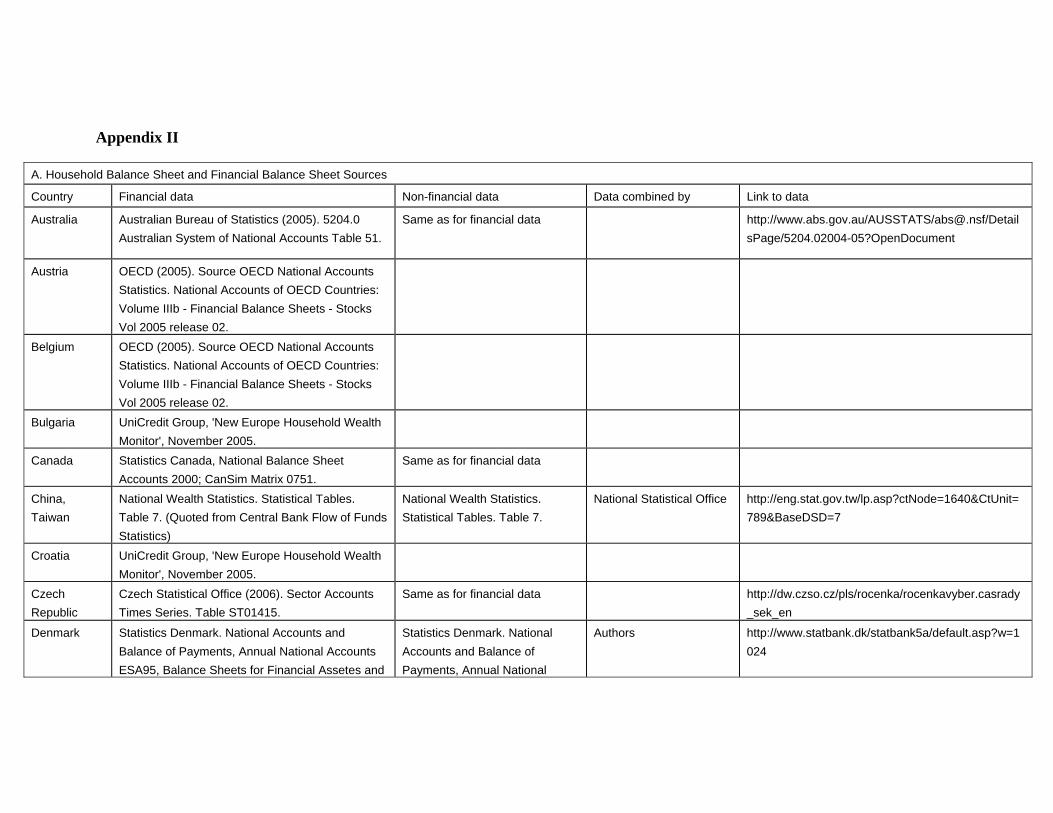
Appendix II

A. Household Balance Sheet and Financial Balance Sheet Sources

Country Financial data Non-financial data Data combined by Link to data

Australia Australian Bureau of Statistics (2005). 5204.0 Australian System of National Accounts Table 51.

Same as for financial data http://www.abs.gov.au/AUSSTATS/abs@.nsf/DetailsPage/5204.02004-05?OpenDocument

Austria OECD (2005). Source OECD National Accounts Statistics. National Accounts of OECD Countries: Volume IIIb - Financial Balance Sheets - Stocks Vol 2005 release 02.

Belgium OECD (2005). Source OECD National Accounts Statistics. National Accounts of OECD Countries: Volume IIIb - Financial Balance Sheets - Stocks Vol 2005 release 02.

Bulgaria UniCredit Group, 'New Europe Household Wealth Monitor', November 2005.

Canada Statistics Canada, National Balance Sheet Accounts 2000; CanSim Matrix 0751.

Same as for financial data

China, Taiwan

National Wealth Statistics. Statistical Tables. Table 7. (Quoted from Central Bank Flow of Funds Statistics)

National Wealth Statistics. Statistical Tables. Table 7.

National Statistical Office http://eng.stat.gov.tw/lp.asp?ctNode=1640&CtUnit=789&BaseDSD=7

Croatia UniCredit Group, 'New Europe Household Wealth Monitor', November 2005.

Czech Republic

Czech Statistical Office (2006). Sector Accounts Times Series. Table ST01415.

Same as for financial data http://dw.czso.cz/pls/rocenka/rocenkavyber.casrady_sek_en

Denmark Statistics Denmark. National Accounts and Balance of Payments, Annual National Accounts ESA95, Balance Sheets for Financial Assetes and

Statistics Denmark. National Accounts and Balance of Payments, Annual National

Authors http://www.statbank.dk/statbank5a/default.asp?w=1024

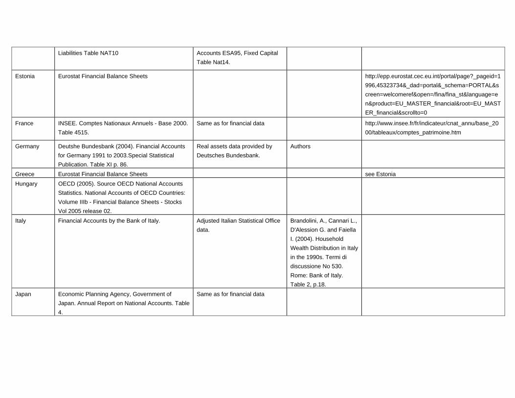
Liabilities Table NAT10 Accounts ESA95, Fixed Capital Table Nat14.

Estonia Eurostat Financial Balance Sheets http://epp.eurostat.cec.eu.int/portal/page?_pageid=1996,45323734&_dad=portal&_schema=PORTAL&screen=welcomeref&open=/fina/fina_st&language=en&product=EU_MASTER_financial&root=EU_MASTER_financial&scrollto=0

France INSEE. Comptes Nationaux Annuels - Base 2000. Table 4515.

Same as for financial data http://www.insee.fr/fr/indicateur/cnat_annu/base_2000/tableaux/comptes_patrimoine.htm

Germany Deutshe Bundesbank (2004). Financial Accounts for Germany 1991 to 2003.Special Statistical Publication. Table XI p. 86.

Real assets data provided by Deutsches Bundesbank.

Authors

Greece Eurostat Financial Balance Sheets see Estonia Hungary OECD (2005). Source OECD National Accounts

Statistics. National Accounts of OECD Countries: Volume IIIb - Financial Balance Sheets - Stocks Vol 2005 release 02.

Italy Financial Accounts by the Bank of Italy. Adjusted Italian Statistical Office data.

Brandolini, A., Cannari L., D'Alession G. and Faiella I. (2004). Household Wealth Distribution in Italy in the 1990s. Termi di discussione No 530. Rome: Bank of Italy. Table 2, p.18.

Japan Economic Planning Agency, Government of Japan. Annual Report on National Accounts. Table 4.

Same as for financial data

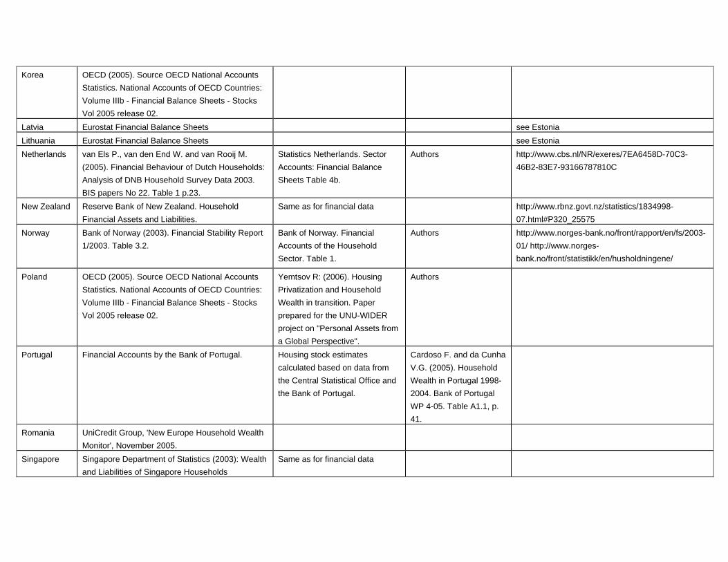
Korea OECD (2005). Source OECD National Accounts Statistics. National Accounts of OECD Countries: Volume IIIb - Financial Balance Sheets - Stocks Vol 2005 release 02.

Latvia Eurostat Financial Balance Sheets see Estonia Lithuania Eurostat Financial Balance Sheets see Estonia Netherlands van Els P., van den End W. and van Rooij M.

(2005). Financial Behaviour of Dutch Households: Analysis of DNB Household Survey Data 2003. BIS papers No 22. Table 1 p.23.

Statistics Netherlands. Sector Accounts: Financial Balance Sheets Table 4b.

Authors http://www.cbs.nl/NR/exeres/7EA6458D-70C3-46B2-83E7-93166787810C

New Zealand Reserve Bank of New Zealand. Household Financial Assets and Liabilities.

Same as for financial data http://www.rbnz.govt.nz/statistics/1834998-07.html#P320_25575

Norway Bank of Norway (2003). Financial Stability Report 1/2003. Table 3.2.

Bank of Norway. Financial Accounts of the Household Sector. Table 1.

Authors http://www.norges-bank.no/front/rapport/en/fs/2003-01/ http://www.norges-bank.no/front/statistikk/en/husholdningene/

Poland OECD (2005). Source OECD National Accounts Statistics. National Accounts of OECD Countries: Volume IIIb - Financial Balance Sheets - Stocks Vol 2005 release 02.

Yemtsov R: (2006). Housing Privatization and Household Wealth in transition. Paper prepared for the UNU-WIDER project on "Personal Assets from a Global Perspective".

Authors

Portugal Financial Accounts by the Bank of Portugal. Housing stock estimates calculated based on data from the Central Statistical Office and the Bank of Portugal.

Cardoso F. and da Cunha V.G. (2005). Household Wealth in Portugal 1998-2004. Bank of Portugal WP 4-05. Table A1.1, p. 41.

Romania UniCredit Group, 'New Europe Household Wealth Monitor', November 2005.

Singapore Singapore Department of Statistics (2003): Wealth and Liabilities of Singapore Households

Same as for financial data

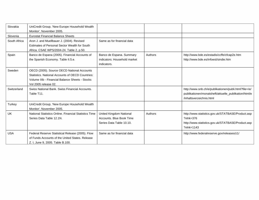
Slovakia UniCredit Group, 'New Europe Household Wealth Monitor', November 2005.

Slovenia Eurostat Financial Balance Sheets South Africa Aron J. and Muellbauer J. (2004). Revised

Estimates of Personal Sector Wealth for South Africa. CSAE WPS/2004-24. Table 2, p.50.

Same as for financial data

Spain Banco de Espana (2005). Financial Accounts of the Spanish Economy. Table II.5.e.

Banco de Espana. Summary indicators: Household market indicators.

Authors http://www.bde.es/estadis/ccffe/cfcap2e.htm http://www.bde.es/infoest/sindie.htm

Sweden OECD (2005). Source OECD National Accounts Statistics. National Accounts of OECD Countries: Volume IIIb - Financial Balance Sheets - Stocks Vol 2005 release 02.

Switzerland Swiss National Bank. Swiss Financial Accounts. Table T11.

http://www.snb.ch/e/publikationen/publi.html?file=/e/publikationen/monatsheft/aktuelle_publikation/html/e/inhaltsverzeichnis.html

Turkey UniCredit Group, 'New Europe Household Wealth Monitor', November 2005.

UK National Statistics Online. Financial Statistics Time Series Data Table 12.1N.

United Kingdom National Accounts. Blue Book Time Series Data Table 10.10.

Authors http://www.statistics.gov.uk/STATBASE/Product.asp?vlnk=376 http://www.statistics.gov.uk/STATBASE/Product.asp?vlnk=1143

USA Federal Reserve Statistical Release (2005). Flow of Funds Accounts of the United States. Release Z. I, June 9, 2005. Table B.100.

Same as for financial data http://www.federalreserve.gov/releases/z1/

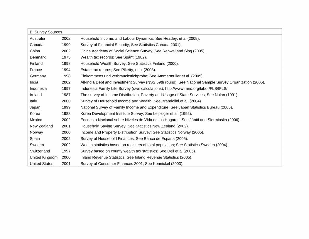
B. Survey Sources Australia 2002 Household Income, and Labour Dynamics; See Headey, et al (2005). Canada 1999 Survey of Financial Security; See Statistics Canada 2001). China 2002 China Academy of Social Science Survey; See Renwei and Sing (2005). Denmark 1975 Wealth tax records; See Spånt (1982). Finland 1998 Household Wealth Survey; See Statistics Finland (2000). France 1994 Estate tax returns; See Piketty, et al (2003). Germany 1998 Einkommens und verbrauchstichprobe; See Ammermuller et al. (2005). India 2002 All-India Debt and Investment Survey (NSS 59th round); See National Sample Survey Organization (2005). Indonesia 1997 Indonesia Family Life Survey (own calculations); http://www.rand.org/labor/FLS/IFLS/ Ireland 1987 The survey of Income Distribution, Poverty and Usage of State Services; See Nolan (1991). Italy 2000 Survey of Household Income and Wealth; See Brandolini et al. (2004). Japan 1999 National Survey of Family Income and Expenditure; See Japan Statistics Bureau (2005). Korea 1988 Korea Development Institute Survey; See Leipziger et al. (1992). Mexico 2002 Encuesta Nacional sobre Niveles de Vida de los Hogares; See Jäntti and Sierminska (2006). New Zealand 2001 Household Saving Survey; See Statistics New Zealand (2002). Norway 2000 Income and Property Distribution Survey; See Statistics Norway (2005). Spain 2002 Survey of Household Finances; See Banco de Espana (2005). Sweden 2002 Wealth statistics based on registers of total population; See Statistics Sweden (2004). Switzerland 1997 Survey based on county wealth tax statistics; See Dell et al (2005). United Kingdom 2000 Inland Revenue Statistics; See Inland Revenue Statistics (2005). United States 2001 Survey of Consumer Finances 2001; See Kennickel (2003).

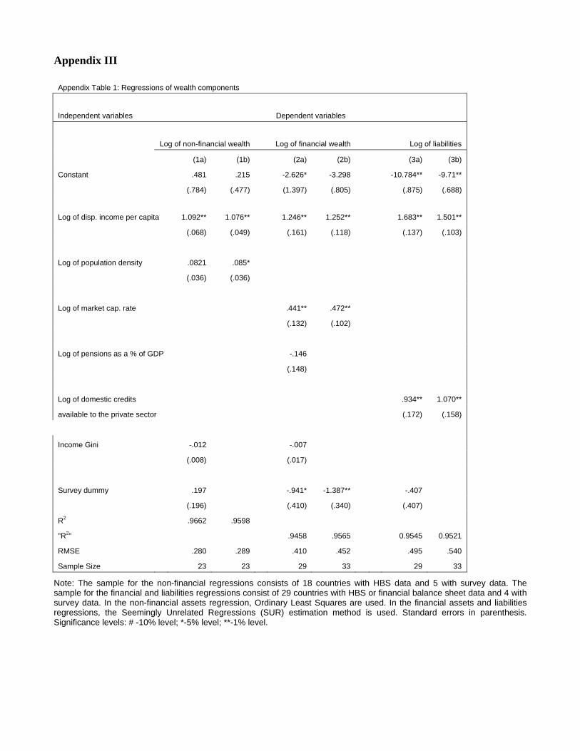
Appendix III

Appendix Table 1: Regressions of wealth components

Independent variables Dependent variables

Log of non-financial wealth Log of financial wealth Log of liabilities

(1a) (1b) (2a) (2b) (3a) (3b)

Constant .481 .215 -2.626* -3.298 -10.784** -9.71**

(.784) (.477) (1.397) (.805) (.875) (.688)

Log of disp. income per capita 1.092** 1.076** 1.246** 1.252** 1.683** 1.501**

(.068) (.049) (.161) (.118) (.137) (.103)

Log of population density .0821 .085*

(.036) (.036)

Log of market cap. rate .441** .472**

(.132) (.102)

Log of pensions as a % of GDP -.146

(.148)

.934** 1.070** Log of domestic credits

available to the private sector (.172) (.158)

Income Gini -.012 -.007

(.008) (.017)

Survey dummy .197 -.941* -1.387** -.407

(.196) (.410) (.340) (.407)

R2 .9662 .9598

"R2" .9458 .9565 0.9545 0.9521

RMSE .280 .289 .410 .452 .495 .540

Sample Size 23 23 29 33 29 33

Note: The sample for the non-financial regressions consists of 18 countries with HBS data and 5 with survey data. The sample for the financial and liabilities regressions consist of 29 countries with HBS or financial balance sheet data and 4 with survey data. In the non-financial assets regression, Ordinary Least Squares are used. In the financial assets and liabilities regressions, the Seemingly Unrelated Regressions (SUR) estimation method is used. Standard errors in parenthesis. Significance levels: # -10% level; *-5% level; **-1% level.

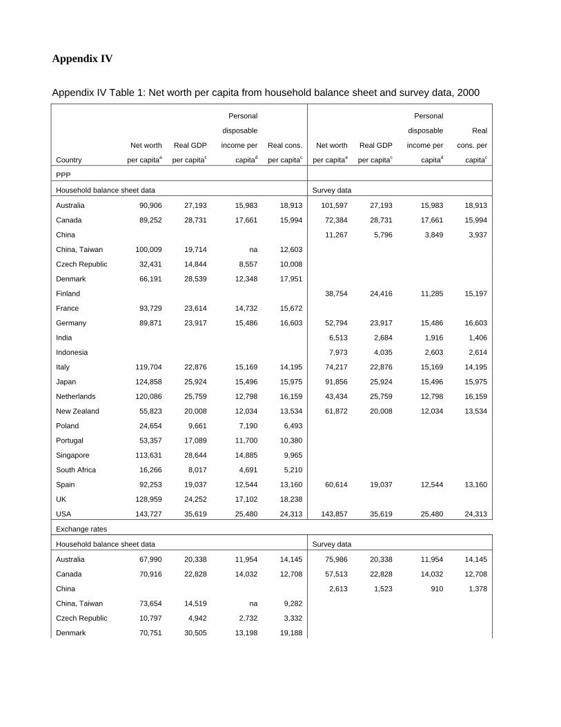
Appendix IV

Appendix IV Table 1: Net worth per capita from household balance sheet and survey data, 2000

Country

Net worth

per capitaa

Real GDP

per capitac

Personal

disposable

income per

capitad

Real cons.

per capitac

Net worth

per capitaa

Real GDP

per capitac

Personal

disposable

income per

capitad

Real

cons. per

capitac

PPP

Household balance sheet data Survey data

Australia 90,906 27,193 15,983 18,913 101,597 27,193 15,983 18,913

Canada 89,252 28,731 17,661 15,994 72,384 28,731 17,661 15,994

China 11,267 5,796 3,849 3,937

China, Taiwan 100,009 19,714 na 12,603

Czech Republic 32,431 14,844 8,557 10,008

Denmark 66,191 28,539 12,348 17,951

Finland 38,754 24,416 11,285 15,197

France 93,729 23,614 14,732 15,672

Germany 89,871 23,917 15,486 16,603 52,794 23,917 15,486 16,603

India 6,513 2,684 1,916 1,406

Indonesia 7,973 4,035 2,603 2,614

Italy 119,704 22,876 15,169 14,195 74,217 22,876 15,169 14,195

Japan 124,858 25,924 15,496 15,975 91,856 25,924 15,496 15,975

Netherlands 120,086 25,759 12,798 16,159 43,434 25,759 12,798 16,159

New Zealand 55,823 20,008 12,034 13,534 61,872 20,008 12,034 13,534

Poland 24,654 9,661 7,190 6,493

Portugal 53,357 17,089 11,700 10,380

Singapore 113,631 28,644 14,885 9,965

South Africa 16,266 8,017 4,691 5,210

Spain 92,253 19,037 12,544 13,160 60,614 19,037 12,544 13,160

UK 128,959 24,252 17,102 18,238

USA 143,727 35,619 25,480 24,313 143,857 35,619 25,480 24,313

Exchange rates

Household balance sheet data Survey data

Australia 67,990 20,338 11,954 14,145 75,986 20,338 11,954 14,145

Canada 70,916 22,828 14,032 12,708 57,513 22,828 14,032 12,708

China 2,613 1,523 910 1,378

China, Taiwan 73,654 14,519 na 9,282

Czech Republic 10,797 4,942 2,732 3,332

Denmark 70,751 30,505 13,198 19,188

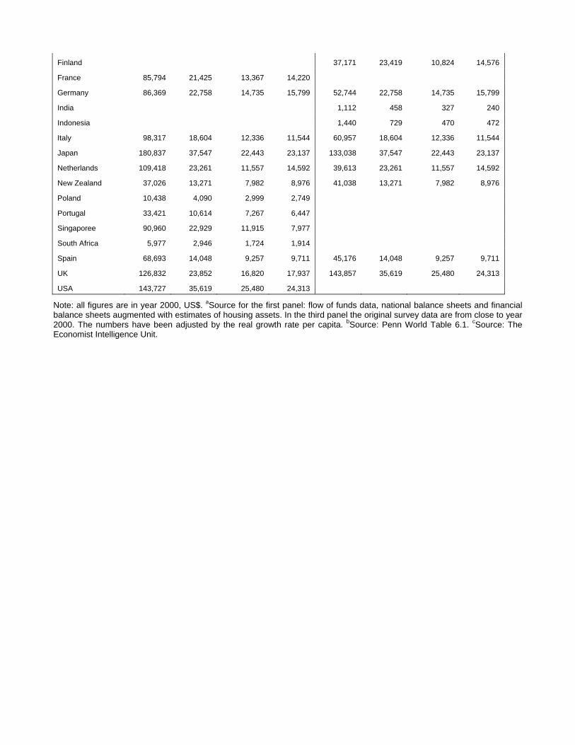
Finland 37,171 23,419 10,824 14,576

France 85,794 21,425 13,367 14,220

Germany 86,369 22,758 14,735 15,799 52,744 22,758 14,735 15,799

India 1,112 458 327 240

Indonesia 1,440 729 470 472

Italy 98,317 18,604 12,336 11,544 60,957 18,604 12,336 11,544

Japan 180,837 37,547 22,443 23,137 133,038 37,547 22,443 23,137

Netherlands 109,418 23,261 11,557 14,592 39,613 23,261 11,557 14,592

New Zealand 37,026 13,271 7,982 8,976 41,038 13,271 7,982 8,976

Poland 10,438 4,090 2,999 2,749

Portugal 33,421 10,614 7,267 6,447

Singaporee 90,960 22,929 11,915 7,977

South Africa 5,977 2,946 1,724 1,914

Spain 68,693 14,048 9,257 9,711 45,176 14,048 9,257 9,711

UK 126,832 23,852 16,820 17,937 143,857 35,619 25,480 24,313

USA 143,727 35,619 25,480 24,313

Note: all figures are in year 2000, US$. aSource for the first panel: flow of funds data, national balance sheets and financial balance sheets augmented with estimates of housing assets. In the third panel the original survey data are from close to year 2000. The numbers have been adjusted by the real growth rate per capita. bSource: Penn World Table 6.1. cSource: The Economist Intelligence Unit.

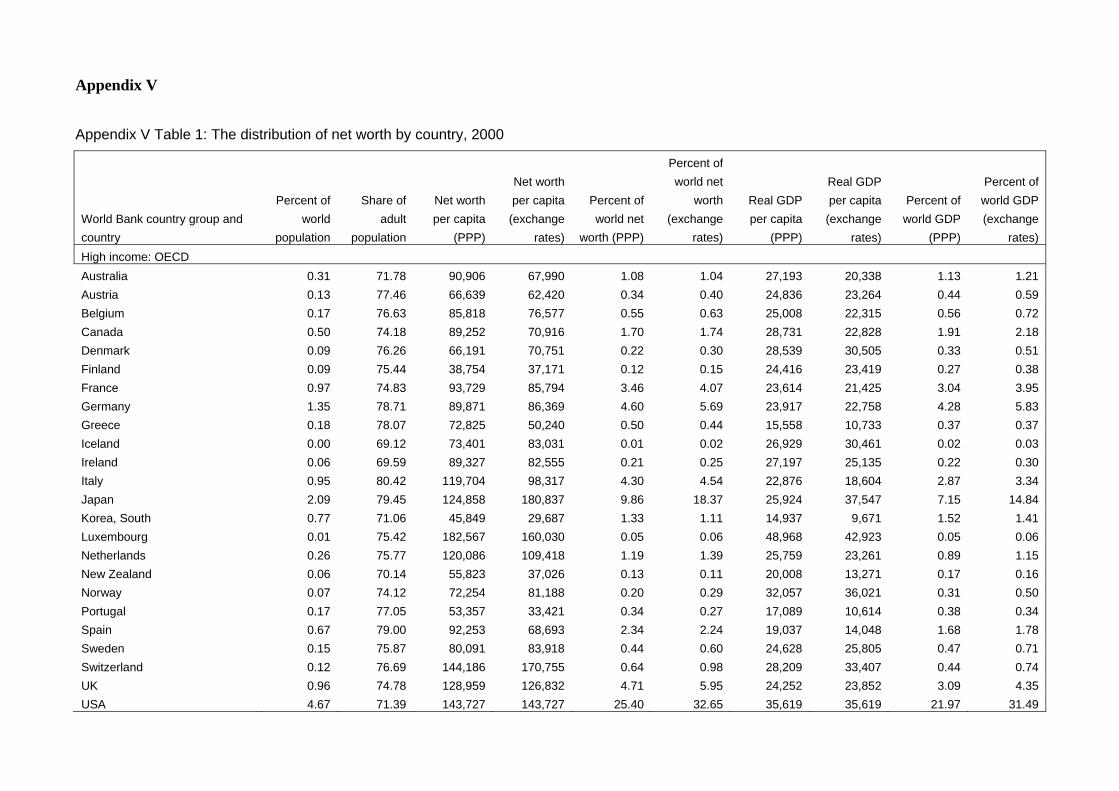
Appendix V

Appendix V Table 1: The distribution of net worth by country, 2000

World Bank country group and country

Percent of world

population

Share of adult

population

Net worth per capita

(PPP)

Net worth per capita (exchange

rates)

Percent of world net

worth (PPP)

Percent of world net

worth (exchange

rates)

Real GDP per capita

(PPP)

Real GDP per capita (exchange

rates)

Percent of world GDP

(PPP)

Percent of world GDP (exchange

rates) High income: OECD Australia 0.31 71.78 90,906 67,990 1.08 1.04 27,193 20,338 1.13 1.21 Austria 0.13 77.46 66,639 62,420 0.34 0.40 24,836 23,264 0.44 0.59 Belgium 0.17 76.63 85,818 76,577 0.55 0.63 25,008 22,315 0.56 0.72 Canada 0.50 74.18 89,252 70,916 1.70 1.74 28,731 22,828 1.91 2.18 Denmark 0.09 76.26 66,191 70,751 0.22 0.30 28,539 30,505 0.33 0.51 Finland 0.09 75.44 38,754 37,171 0.12 0.15 24,416 23,419 0.27 0.38 France 0.97 74.83 93,729 85,794 3.46 4.07 23,614 21,425 3.04 3.95 Germany 1.35 78.71 89,871 86,369 4.60 5.69 23,917 22,758 4.28 5.83 Greece 0.18 78.07 72,825 50,240 0.50 0.44 15,558 10,733 0.37 0.37 Iceland 0.00 69.12 73,401 83,031 0.01 0.02 26,929 30,461 0.02 0.03 Ireland 0.06 69.59 89,327 82,555 0.21 0.25 27,197 25,135 0.22 0.30 Italy 0.95 80.42 119,704 98,317 4.30 4.54 22,876 18,604 2.87 3.34 Japan 2.09 79.45 124,858 180,837 9.86 18.37 25,924 37,547 7.15 14.84 Korea, South 0.77 71.06 45,849 29,687 1.33 1.11 14,937 9,671 1.52 1.41 Luxembourg 0.01 75.42 182,567 160,030 0.05 0.06 48,968 42,923 0.05 0.06 Netherlands 0.26 75.77 120,086 109,418 1.19 1.39 25,759 23,261 0.89 1.15 New Zealand 0.06 70.14 55,823 37,026 0.13 0.11 20,008 13,271 0.17 0.16 Norway 0.07 74.12 72,254 81,188 0.20 0.29 32,057 36,021 0.31 0.50 Portugal 0.17 77.05 53,357 33,421 0.34 0.27 17,089 10,614 0.38 0.34 Spain 0.67 79.00 92,253 68,693 2.34 2.24 19,037 14,048 1.68 1.78 Sweden 0.15 75.87 80,091 83,918 0.44 0.60 24,628 25,805 0.47 0.71 Switzerland 0.12 76.69 144,186 170,755 0.64 0.98 28,209 33,407 0.44 0.74 UK 0.96 74.78 128,959 126,832 4.71 5.95 24,252 23,852 3.09 4.35 USA 4.67 71.39 143,727 143,727 25.40 32.65 35,619 35,619 21.97 31.49

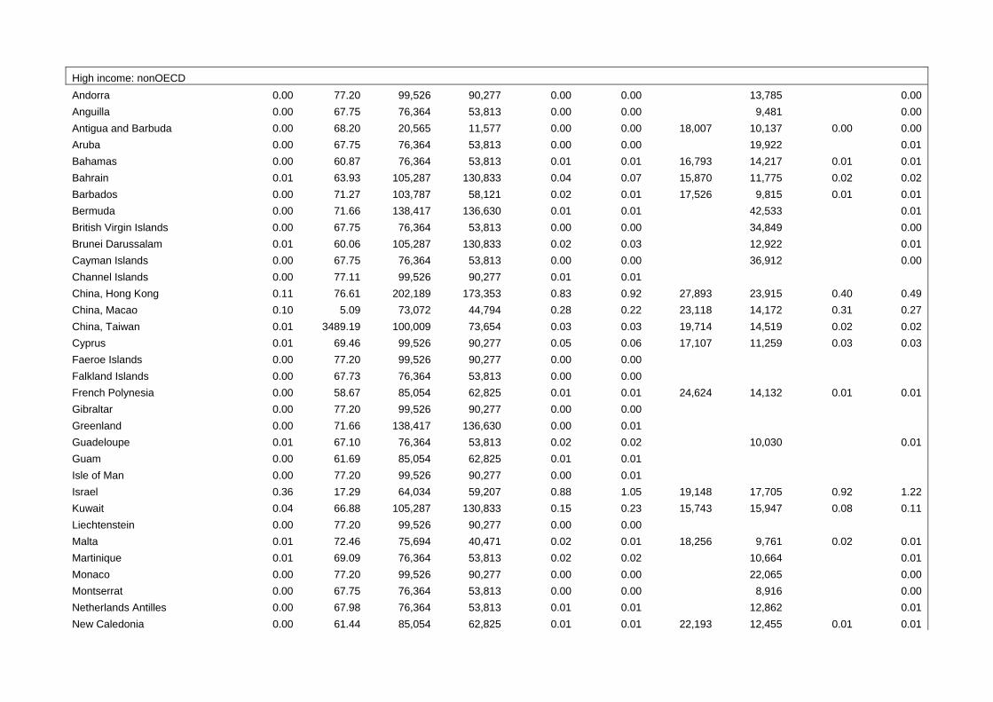
High income: nonOECD Andorra 0.00 77.20 99,526 90,277 0.00 0.00 13,785 0.00 Anguilla 0.00 67.75 76,364 53,813 0.00 0.00 9,481 0.00 Antigua and Barbuda 0.00 68.20 20,565 11,577 0.00 0.00 18,007 10,137 0.00 0.00 Aruba 0.00 67.75 76,364 53,813 0.00 0.00 19,922 0.01 Bahamas 0.00 60.87 76,364 53,813 0.01 0.01 16,793 14,217 0.01 0.01 Bahrain 0.01 63.93 105,287 130,833 0.04 0.07 15,870 11,775 0.02 0.02 Barbados 0.00 71.27 103,787 58,121 0.02 0.01 17,526 9,815 0.01 0.01 Bermuda 0.00 71.66 138,417 136,630 0.01 0.01 42,533 0.01 British Virgin Islands 0.00 67.75 76,364 53,813 0.00 0.00 34,849 0.00 Brunei Darussalam 0.01 60.06 105,287 130,833 0.02 0.03 12,922 0.01 Cayman Islands 0.00 67.75 76,364 53,813 0.00 0.00 36,912 0.00 Channel Islands 0.00 77.11 99,526 90,277 0.01 0.01 China, Hong Kong 0.11 76.61 202,189 173,353 0.83 0.92 27,893 23,915 0.40 0.49 China, Macao 0.10 5.09 73,072 44,794 0.28 0.22 23,118 14,172 0.31 0.27 China, Taiwan 0.01 3489.19 100,009 73,654 0.03 0.03 19,714 14,519 0.02 0.02 Cyprus 0.01 69.46 99,526 90,277 0.05 0.06 17,107 11,259 0.03 0.03 Faeroe Islands 0.00 77.20 99,526 90,277 0.00 0.00 Falkland Islands 0.00 67.73 76,364 53,813 0.00 0.00 French Polynesia 0.00 58.67 85,054 62,825 0.01 0.01 24,624 14,132 0.01 0.01 Gibraltar 0.00 77.20 99,526 90,277 0.00 0.00 Greenland 0.00 71.66 138,417 136,630 0.00 0.01 Guadeloupe 0.01 67.10 76,364 53,813 0.02 0.02 10,030 0.01 Guam 0.00 61.69 85,054 62,825 0.01 0.01 Isle of Man 0.00 77.20 99,526 90,277 0.00 0.01 Israel 0.36 17.29 64,034 59,207 0.88 1.05 19,148 17,705 0.92 1.22 Kuwait 0.04 66.88 105,287 130,833 0.15 0.23 15,743 15,947 0.08 0.11 Liechtenstein 0.00 77.20 99,526 90,277 0.00 0.00 Malta 0.01 72.46 75,694 40,471 0.02 0.01 18,256 9,761 0.02 0.01 Martinique 0.01 69.09 76,364 53,813 0.02 0.02 10,664 0.01 Monaco 0.00 77.20 99,526 90,277 0.00 0.00 22,065 0.00 Montserrat 0.00 67.75 76,364 53,813 0.00 0.00 8,916 0.00 Netherlands Antilles 0.00 67.98 76,364 53,813 0.01 0.01 12,862 0.01 New Caledonia 0.00 61.44 85,054 62,825 0.01 0.01 22,193 12,455 0.01 0.01

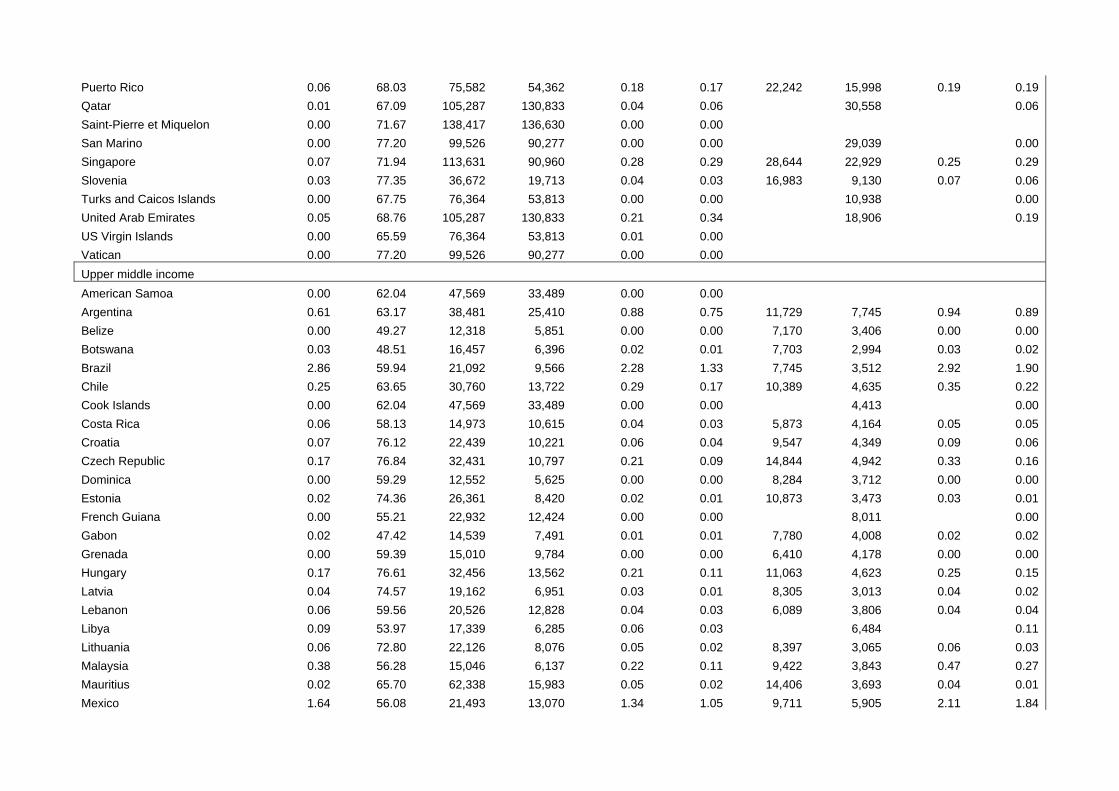
Puerto Rico 0.06 68.03 75,582 54,362 0.18 0.17 22,242 15,998 0.19 0.19 Qatar 0.01 67.09 105,287 130,833 0.04 0.06 30,558 0.06 Saint-Pierre et Miquelon 0.00 71.67 138,417 136,630 0.00 0.00 San Marino 0.00 77.20 99,526 90,277 0.00 0.00 29,039 0.00 Singapore 0.07 71.94 113,631 90,960 0.28 0.29 28,644 22,929 0.25 0.29 Slovenia 0.03 77.35 36,672 19,713 0.04 0.03 16,983 9,130 0.07 0.06 Turks and Caicos Islands 0.00 67.75 76,364 53,813 0.00 0.00 10,938 0.00 United Arab Emirates 0.05 68.76 105,287 130,833 0.21 0.34 18,906 0.19 US Virgin Islands 0.00 65.59 76,364 53,813 0.01 0.00 Vatican 0.00 77.20 99,526 90,277 0.00 0.00 Upper middle income American Samoa 0.00 62.04 47,569 33,489 0.00 0.00 Argentina 0.61 63.17 38,481 25,410 0.88 0.75 11,729 7,745 0.94 0.89 Belize 0.00 49.27 12,318 5,851 0.00 0.00 7,170 3,406 0.00 0.00 Botswana 0.03 48.51 16,457 6,396 0.02 0.01 7,703 2,994 0.03 0.02 Brazil 2.86 59.94 21,092 9,566 2.28 1.33 7,745 3,512 2.92 1.90 Chile 0.25 63.65 30,760 13,722 0.29 0.17 10,389 4,635 0.35 0.22 Cook Islands 0.00 62.04 47,569 33,489 0.00 0.00 4,413 0.00 Costa Rica 0.06 58.13 14,973 10,615 0.04 0.03 5,873 4,164 0.05 0.05 Croatia 0.07 76.12 22,439 10,221 0.06 0.04 9,547 4,349 0.09 0.06 Czech Republic 0.17 76.84 32,431 10,797 0.21 0.09 14,844 4,942 0.33 0.16 Dominica 0.00 59.29 12,552 5,625 0.00 0.00 8,284 3,712 0.00 0.00 Estonia 0.02 74.36 26,361 8,420 0.02 0.01 10,873 3,473 0.03 0.01 French Guiana 0.00 55.21 22,932 12,424 0.00 0.00 8,011 0.00 Gabon 0.02 47.42 14,539 7,491 0.01 0.01 7,780 4,008 0.02 0.02 Grenada 0.00 59.39 15,010 9,784 0.00 0.00 6,410 4,178 0.00 0.00 Hungary 0.17 76.61 32,456 13,562 0.21 0.11 11,063 4,623 0.25 0.15 Latvia 0.04 74.57 19,162 6,951 0.03 0.01 8,305 3,013 0.04 0.02 Lebanon 0.06 59.56 20,526 12,828 0.04 0.03 6,089 3,806 0.04 0.04 Libya 0.09 53.97 17,339 6,285 0.06 0.03 6,484 0.11 Lithuania 0.06 72.80 22,126 8,076 0.05 0.02 8,397 3,065 0.06 0.03 Malaysia 0.38 56.28 15,046 6,137 0.22 0.11 9,422 3,843 0.47 0.27 Mauritius 0.02 65.70 62,338 15,983 0.05 0.02 14,406 3,693 0.04 0.01 Mexico 1.64 56.08 21,493 13,070 1.34 1.05 9,711 5,905 2.11 1.84

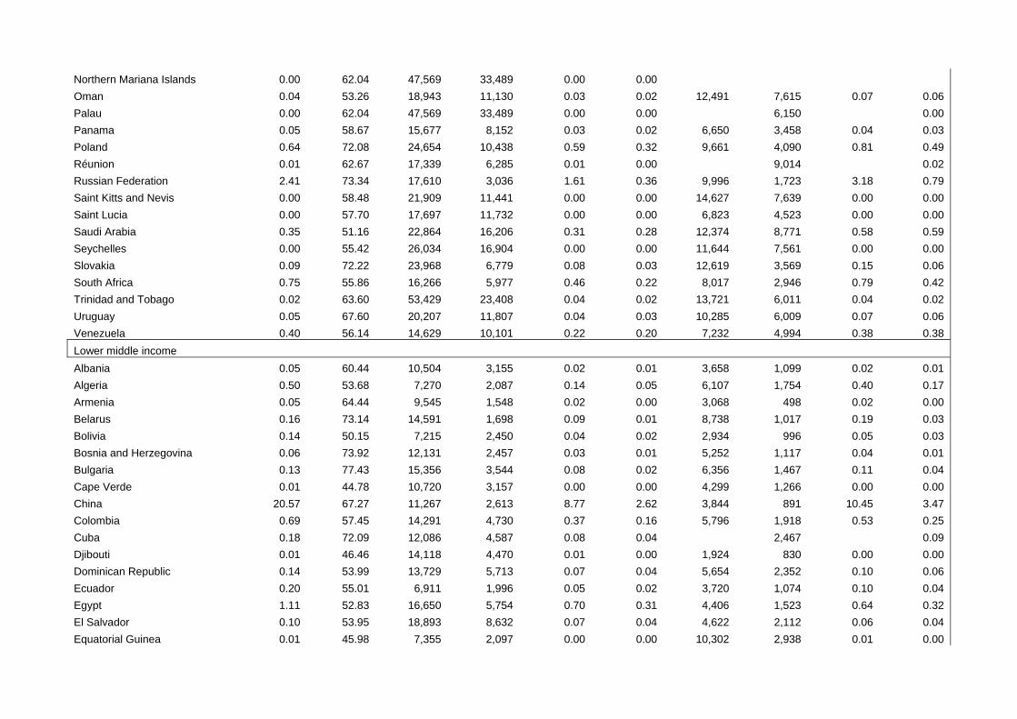
Northern Mariana Islands 0.00 62.04 47,569 33,489 0.00 0.00 Oman 0.04 53.26 18,943 11,130 0.03 0.02 12,491 7,615 0.07 0.06 Palau 0.00 62.04 47,569 33,489 0.00 0.00 6,150 0.00 Panama 0.05 58.67 15,677 8,152 0.03 0.02 6,650 3,458 0.04 0.03 Poland 0.64 72.08 24,654 10,438 0.59 0.32 9,661 4,090 0.81 0.49 Réunion 0.01 62.67 17,339 6,285 0.01 0.00 9,014 0.02 Russian Federation 2.41 73.34 17,610 3,036 1.61 0.36 9,996 1,723 3.18 0.79 Saint Kitts and Nevis 0.00 58.48 21,909 11,441 0.00 0.00 14,627 7,639 0.00 0.00 Saint Lucia 0.00 57.70 17,697 11,732 0.00 0.00 6,823 4,523 0.00 0.00 Saudi Arabia 0.35 51.16 22,864 16,206 0.31 0.28 12,374 8,771 0.58 0.59 Seychelles 0.00 55.42 26,034 16,904 0.00 0.00 11,644 7,561 0.00 0.00 Slovakia 0.09 72.22 23,968 6,779 0.08 0.03 12,619 3,569 0.15 0.06 South Africa 0.75 55.86 16,266 5,977 0.46 0.22 8,017 2,946 0.79 0.42 Trinidad and Tobago 0.02 63.60 53,429 23,408 0.04 0.02 13,721 6,011 0.04 0.02 Uruguay 0.05 67.60 20,207 11,807 0.04 0.03 10,285 6,009 0.07 0.06 Venezuela 0.40 56.14 14,629 10,101 0.22 0.20 7,232 4,994 0.38 0.38 Lower middle income Albania 0.05 60.44 10,504 3,155 0.02 0.01 3,658 1,099 0.02 0.01 Algeria 0.50 53.68 7,270 2,087 0.14 0.05 6,107 1,754 0.40 0.17 Armenia 0.05 64.44 9,545 1,548 0.02 0.00 3,068 498 0.02 0.00 Belarus 0.16 73.14 14,591 1,698 0.09 0.01 8,738 1,017 0.19 0.03 Bolivia 0.14 50.15 7,215 2,450 0.04 0.02 2,934 996 0.05 0.03 Bosnia and Herzegovina 0.06 73.92 12,131 2,457 0.03 0.01 5,252 1,117 0.04 0.01 Bulgaria 0.13 77.43 15,356 3,544 0.08 0.02 6,356 1,467 0.11 0.04 Cape Verde 0.01 44.78 10,720 3,157 0.00 0.00 4,299 1,266 0.00 0.00 China 20.57 67.27 11,267 2,613 8.77 2.62 3,844 891 10.45 3.47 Colombia 0.69 57.45 14,291 4,730 0.37 0.16 5,796 1,918 0.53 0.25 Cuba 0.18 72.09 12,086 4,587 0.08 0.04 2,467 0.09 Djibouti 0.01 46.46 14,118 4,470 0.01 0.00 1,924 830 0.00 0.00 Dominican Republic 0.14 53.99 13,729 5,713 0.07 0.04 5,654 2,352 0.10 0.06 Ecuador 0.20 55.01 6,911 1,996 0.05 0.02 3,720 1,074 0.10 0.04 Egypt 1.11 52.83 16,650 5,754 0.70 0.31 4,406 1,523 0.64 0.32 El Salvador 0.10 53.95 18,893 8,632 0.07 0.04 4,622 2,112 0.06 0.04 Equatorial Guinea 0.01 45.98 7,355 2,097 0.00 0.00 10,302 2,938 0.01 0.00

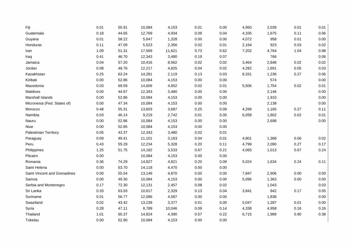
Fiji 0.01 55.91 10,084 4,153 0.01 0.00 4,950 2,039 0.01 0.01 Guatemala 0.18 44.65 12,769 4,934 0.09 0.04 4,335 1,675 0.11 0.06 Guyana 0.01 58.22 5,647 1,328 0.00 0.00 4,072 958 0.01 0.00 Honduras 0.11 47.09 5,523 2,356 0.02 0.01 2,164 923 0.03 0.02 Iran 1.09 51.31 17,569 11,621 0.73 0.62 7,202 4,764 1.04 0.98 Iraq 0.41 46.70 12,343 3,480 0.19 0.07 766 0.06 Jamaica 0.04 57.20 10,416 8,562 0.02 0.02 3,464 2,848 0.02 0.02 Jordan 0.08 49.76 12,217 4,825 0.04 0.02 4,282 1,691 0.05 0.03 Kazakhstan 0.25 63.24 14,281 2,119 0.13 0.03 8,331 1,236 0.27 0.06 Kiribati 0.00 52.86 10,084 4,153 0.00 0.00 574 0.00 Macedonia 0.03 69.59 14,606 4,652 0.02 0.01 5,506 1,754 0.02 0.01 Maldives 0.00 44.67 12,343 3,480 0.00 0.00 2,146 0.00 Marshall Islands 0.00 52.86 10,084 4,153 0.00 0.00 1,910 0.00 Micronesia (Fed. States of) 0.00 47.34 10,084 4,153 0.00 0.00 2,138 0.00 Morocco 0.48 55.31 13,603 3,687 0.25 0.09 4,299 1,165 0.27 0.11 Namibia 0.03 46.14 9,219 2,742 0.01 0.00 6,058 1,802 0.02 0.01 Nauru 0.00 52.86 10,084 4,153 0.00 0.00 2,698 0.00 Niue 0.00 52.85 10,084 4,153 0.00 0.00 Palestinian Territory 0.05 43.37 12,343 3,480 0.02 0.01 Paraguay 0.09 49.41 11,101 3,163 0.04 0.01 4,801 1,368 0.06 0.02 Peru 0.43 55.29 12,234 5,328 0.20 0.11 4,799 2,090 0.27 0.17 Philippines 1.25 51.75 14,182 3,533 0.67 0.21 4,065 1,013 0.67 0.24 Pitcairn 0.00 10,084 4,153 0.00 0.00 Romania 0.36 74.29 14,827 4,821 0.20 0.09 5,024 1,634 0.24 0.11 Saint Helena 0.00 53.70 14,118 4,470 0.00 0.00 Saint Vincent and Grenadines 0.00 55.54 13,149 4,870 0.00 0.00 7,847 2,906 0.00 0.00 Samoa 0.00 49.30 10,084 4,153 0.00 0.00 5,096 1,363 0.00 0.00 Serbia and Montenegro 0.17 72.30 12,131 2,457 0.08 0.02 1,043 0.03 Sri Lanka 0.33 63.93 10,617 2,329 0.13 0.04 3,841 842 0.17 0.05 Suriname 0.01 56.77 12,086 4,587 0.00 0.00 1,838 0.00 Swaziland 0.02 43.42 13,239 3,377 0.01 0.00 5,047 1,287 0.01 0.00 Syria 0.28 47.11 8,789 10,046 0.09 0.14 4,338 4,958 0.16 0.26 Thailand 1.01 65.37 14,824 4,390 0.57 0.22 6,715 1,989 0.90 0.38 Tokelau 0.00 52.90 10,084 4,153 0.00 0.00

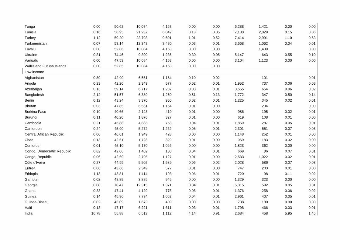
Tonga 0.00 50.62 10,084 4,153 0.00 0.00 6,288 1,421 0.00 0.00 Tunisia 0.16 58.95 21,237 6,042 0.13 0.05 7,130 2,029 0.15 0.06 Turkey 1.12 59.20 23,798 9,601 1.01 0.52 7,414 2,991 1.10 0.63 Turkmenistan 0.07 53.14 12,343 3,480 0.03 0.01 3,668 1,062 0.04 0.01 Tuvalu 0.00 52.86 10,084 4,153 0.00 0.00 1,409 0.00 Ukraine 0.81 74.46 9,890 1,236 0.30 0.05 5,147 643 0.55 0.10 Vanuatu 0.00 47.53 10,084 4,153 0.00 0.00 3,104 1,123 0.00 0.00 Wallis and Futuna Islands 0.00 52.85 10,084 4,153 0.00 0.00 Low income Afghanistan 0.39 42.90 6,561 1,164 0.10 0.02 101 0.01 Angola 0.23 42.20 2,349 577 0.02 0.01 1,952 737 0.06 0.03 Azerbaijan 0.13 59.14 6,717 1,237 0.03 0.01 3,555 654 0.06 0.02 Bangladesh 2.12 51.57 6,389 1,250 0.51 0.13 1,772 347 0.50 0.14 Benin 0.12 43.24 3,370 950 0.02 0.01 1,225 345 0.02 0.01 Bhutan 0.03 47.85 6,561 1,164 0.01 0.00 234 0.00 Burkina Faso 0.19 40.66 2,123 419 0.01 0.00 986 195 0.02 0.01 Burundi 0.11 40.20 1,876 327 0.01 0.00 619 108 0.01 0.00 Cambodia 0.21 45.88 4,883 753 0.04 0.01 1,859 287 0.05 0.01 Cameroon 0.24 45.90 5,272 1,262 0.05 0.01 2,301 551 0.07 0.03 Central African Republic 0.06 46.01 1,949 428 0.00 0.00 1,148 252 0.01 0.00 Chad 0.13 42.61 1,728 329 0.01 0.00 959 183 0.02 0.00 Comoros 0.01 45.10 5,170 1,026 0.00 0.00 1,823 362 0.00 0.00 Congo, Democratic Republic 0.82 42.06 1,402 180 0.04 0.01 669 86 0.07 0.01 Congo, Republic 0.06 42.69 2,795 1,127 0.01 0.00 2,533 1,022 0.02 0.01 Côte d'Ivoire 0.27 44.99 5,502 1,589 0.06 0.02 2,028 586 0.07 0.03 Eritrea 0.06 43.66 2,349 577 0.01 0.00 747 203 0.01 0.00 Ethiopia 1.13 43.81 1,414 193 0.06 0.01 720 98 0.11 0.02 Gambia 0.02 48.89 3,885 945 0.00 0.00 1,329 323 0.00 0.00 Georgia 0.08 70.47 12,315 1,371 0.04 0.01 5,315 592 0.05 0.01 Ghana 0.33 47.41 4,129 775 0.05 0.01 1,376 258 0.06 0.02 Guinea 0.14 45.96 7,734 1,062 0.04 0.01 2,961 407 0.05 0.01 Guinea-Bissau 0.02 43.09 1,673 409 0.00 0.00 738 180 0.00 0.00 Haiti 0.13 47.17 6,221 1,611 0.03 0.01 1,798 466 0.03 0.01 India 16.78 55.88 6,513 1,112 4.14 0.91 2,684 458 5.95 1.45

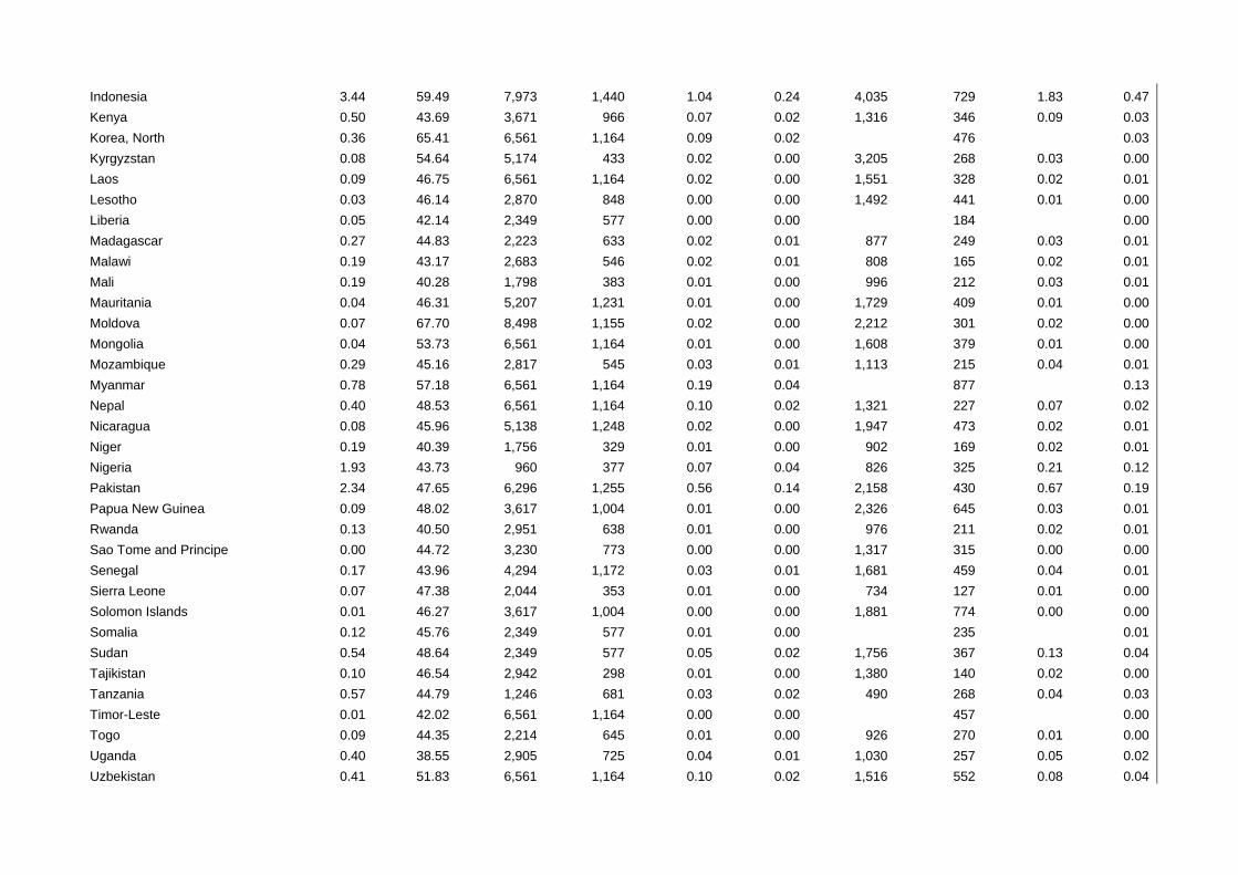
Indonesia 3.44 59.49 7,973 1,440 1.04 0.24 4,035 729 1.83 0.47 Kenya 0.50 43.69 3,671 966 0.07 0.02 1,316 346 0.09 0.03 Korea, North 0.36 65.41 6,561 1,164 0.09 0.02 476 0.03 Kyrgyzstan 0.08 54.64 5,174 433 0.02 0.00 3,205 268 0.03 0.00 Laos 0.09 46.75 6,561 1,164 0.02 0.00 1,551 328 0.02 0.01 Lesotho 0.03 46.14 2,870 848 0.00 0.00 1,492 441 0.01 0.00 Liberia 0.05 42.14 2,349 577 0.00 0.00 184 0.00 Madagascar 0.27 44.83 2,223 633 0.02 0.01 877 249 0.03 0.01 Malawi 0.19 43.17 2,683 546 0.02 0.01 808 165 0.02 0.01 Mali 0.19 40.28 1,798 383 0.01 0.00 996 212 0.03 0.01 Mauritania 0.04 46.31 5,207 1,231 0.01 0.00 1,729 409 0.01 0.00 Moldova 0.07 67.70 8,498 1,155 0.02 0.00 2,212 301 0.02 0.00 Mongolia 0.04 53.73 6,561 1,164 0.01 0.00 1,608 379 0.01 0.00 Mozambique 0.29 45.16 2,817 545 0.03 0.01 1,113 215 0.04 0.01 Myanmar 0.78 57.18 6,561 1,164 0.19 0.04 877 0.13 Nepal 0.40 48.53 6,561 1,164 0.10 0.02 1,321 227 0.07 0.02 Nicaragua 0.08 45.96 5,138 1,248 0.02 0.00 1,947 473 0.02 0.01 Niger 0.19 40.39 1,756 329 0.01 0.00 902 169 0.02 0.01 Nigeria 1.93 43.73 960 377 0.07 0.04 826 325 0.21 0.12 Pakistan 2.34 47.65 6,296 1,255 0.56 0.14 2,158 430 0.67 0.19 Papua New Guinea 0.09 48.02 3,617 1,004 0.01 0.00 2,326 645 0.03 0.01 Rwanda 0.13 40.50 2,951 638 0.01 0.00 976 211 0.02 0.01 Sao Tome and Principe 0.00 44.72 3,230 773 0.00 0.00 1,317 315 0.00 0.00 Senegal 0.17 43.96 4,294 1,172 0.03 0.01 1,681 459 0.04 0.01 Sierra Leone 0.07 47.38 2,044 353 0.01 0.00 734 127 0.01 0.00 Solomon Islands 0.01 46.27 3,617 1,004 0.00 0.00 1,881 774 0.00 0.00 Somalia 0.12 45.76 2,349 577 0.01 0.00 235 0.01 Sudan 0.54 48.64 2,349 577 0.05 0.02 1,756 367 0.13 0.04 Tajikistan 0.10 46.54 2,942 298 0.01 0.00 1,380 140 0.02 0.00 Tanzania 0.57 44.79 1,246 681 0.03 0.02 490 268 0.04 0.03 Timor-Leste 0.01 42.02 6,561 1,164 0.00 0.00 457 0.00 Togo 0.09 44.35 2,214 645 0.01 0.00 926 270 0.01 0.00 Uganda 0.40 38.55 2,905 725 0.04 0.01 1,030 257 0.05 0.02 Uzbekistan 0.41 51.83 6,561 1,164 0.10 0.02 1,516 552 0.08 0.04

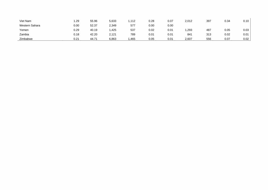
Viet Nam 1.29 55.96 5,633 1,112 0.28 0.07 2,012 397 0.34 0.10 Western Sahara 0.00 52.37 2,349 577 0.00 0.00 Yemen 0.29 40.19 1,425 537 0.02 0.01 1,293 487 0.05 0.03 Zambia 0.18 42.20 2,121 789 0.01 0.01 841 313 0.02 0.01 Zimbabwe 0.21 44.71 6,863 1,465 0.05 0.01 2,607 556 0.07 0.02