The Welfare Consequences of Monetary Policy

and the Role of the Labor Market: a Tax

Interpretation

Federico Ravenna and Carl E. Walsh∗

April 2009

Abstract

We explore the distortions in business cycle models arising from inefficiencies in

price setting and in the search process matching firms to unemployed workers, and

the implications of these distortions for monetary policy. To this end, we characterize

the tax instruments that would implement the first best equilibrium allocations and

then examine the trade-offs faced by monetary policy when these tax instruments are

unavailable. Our findings are that the welfare cost of search inefficiency can be large,

but the incentive for policy to deviate from the inefficient flexible-price allocation is in

general small. Sizable welfare gains are available if the steady state of the economy is

inefficient, and these gains do not depend on the existence of an inefficient dispersion

of wages. Finally, the gains from deviating from price stability are larger in economies

with more volatile labor flows, as in the U.S.

JEL: E52, E58, J64

∗Department of Economics, University of California, Santa Cruz, CA 95064, and Federal Reserve Bankof San Francisco, 101 Market St, San Francisco, CA 94105. Email: fravenna@ucsc.edu, walshc@ucsc.edu.

1

1 Introduction

This paper explores optimal monetary policy in business cycle models with staggered

price adjustment and inefficiencies in the search process that matches job vacancies with

unemployed workers. In this environment the markup in the final-goods producing sector

affects equilibrium through three separate channels. First, it affects the incentive for firms

to post job vacancies. Second, it influences the equilibrium hours per employed worker.

Finally, it affects the marginal cost of retail firms and generates a dispersion of relative

prices. It is feasible for monetary policy to completely undo the distortions associated

with sticky prices and replicate the flexible-price equilibrium. However, such a policy of

price stability cannot ensure efficient outcomes in the labor market. Because monetary

policy can affect the incentive to post vacancies when prices are sticky but not when

prices are flexible, we find that the policymaker can achieve higher welfare in an economy

with staggered price setting than in a flexible-price economy.

At the same time, while the cost of inefficient vacancy posting is large, the welfare

attained by the optimal policy deviates very little from the one achieved under flexible

prices. In practice, the policymaker finds little incentive in trying to correct for the

search inefficiency by deviating from price stability. Introducing real wage rigidity does

not, in itself, modify this result. Finally, we find that a higher cost of search, resulting

in lower steady-state employment, has two opposing effects on policy. Structural policies

addressing labor markets distortions can bring larger gains, but cyclical monetary policy

becomes less effective, thus making the policy implementing the flexible price allocation

a closer approximation to the optimal policy.

The result that replicating the allocation obtained when nominal rigidities are absent

is not optimal is similar to Adao, Correia, Teles (2003), and carries the same intuition.

Real distortions exist that cannot be affected by monetary policy under flexible prices.

Staggered price setting offers the policymaker an instrument to correct for these distor-

tion. The existence of multiple distortions implies that under either flexible or staggered

prices the optimal policy can only attain a second best. Among the second best allo-

cations, it turns out that eliminating one distortion can be welfare decreasing. In our

model, which includes the search and matching labor market of Mortensen and Pissarides

(1994), equilibrium unemployment and vacancies can deviate from their efficient levels,

and a policy of price stability replicates the inefficient equilibrium level of employment

that would obtain with flexible prices. If search in the labor market is inefficient, stag-

gered price setting gives monetary policy the opportunity to correct the incentives of

households and firms and generate an efficient level of employment.

The result that the flexible price allocation may be feasible but suboptimal is well

understood in the literature on monetary policy in the presence of nominal rigidities

(Blanchard and Galí, 2007). Much of this literature though assumes an efficient steady

2

state achieved through fiscal transfers. In this case, eliminating all nominal rigidities

achieves the first best and is always welfare-improving (as in the sticky price and wage

model of Erceg, Henderson and Levin, 2000 or the sticky price-cost channel model of

Ravenna and Walsh, 2006).

Our second set of result sheds light on the nature of the distortions in models with

staggered price setting and labor market frictions. For reasonable model parameteriza-

tions, the welfare loss from search inefficiencies is large under the flexible price allocation.

Thus it appears there is ample space for monetary policy to improve on the allocation

that would obtain by fully stabilizing prices. While this ’search gap’ is large, monetary

policy is able to close only a tiny fraction of it. The monetary policy outcome hinges

both on the wage-setting process and on the efficiency of the steady state. When wages

are Nash-bargained in every period but set at a socially inefficient level, nearly all of the

search gap can be explained by inefficiency in the steady state. This is the welfare impli-

cation of the low relative volatility of employment and output generated by this family of

models (Shimer, 2004): inefficient but small fluctuations of employment result in a small

welfare loss. In this economy, movements in unemployment become virtually a sideshow

as far as the policymaker is concerned: focusing on the inefficiency from nominal rigidities

should be the primary policy concern.

Adding wage rigidities does not, in itself, change this result. With real wages fixed at a

wage norm, the volatility of unemployment increases substantially, and so does the welfare

loss generated by the business cycle. But the trade-off faced by the monetary authority

is extremely unfavorable, so it is optimal not to deviate much from price stability. It

is only with a wage fixed at a level very different from the efficient steady state that

deviations from price stability yield high return in terms of welfare. We find that the

optimal policy can yield welfare gains on the order of one half percent of steady-state

consumption. This improvement derives entirely from correcting for search frictions that

would otherwise prevent an efficient response to technology shocks under the flexible

price allocation. Since it is common in the literature to assume the steady-state wage is

efficient, our results are relevant for interpreting previous findings.

In our framework, monetary policy is of limited effectiveness because it can only affect

markups, and these markups directly affect all of the distortions present in the economy.

In effect, monetary policy is a blunt instrument - and, ironically, especially so when the

cost of search is higher. This is illustrated clearly by our analysis, which maps monetary

policy into a tax policy. We first derive the tax and subsidy policy that would replicate the

efficient, social planner’s equilibrium in an economy with sticky prices, search frictions,

and a labor market that allows adjustment to occur on both the intensive and extensive

margins. We then consider the extent to which monetary policy can mimic this optimal

tax policy. This allows us to focus on the exact nature of the distortions that might call

for deviations from price stability and to quantify the impact of these distortions on the

3

dynamics of the economy over the business cycle.

We find that three policy instruments are generally needed to replicate the efficient

equilibrium. A tax on intermediate firms can ensure efficient vacancy creation. However,

such a tax distorts the hours choice and so a second tax instrument is needed to ensure

that hours are chosen optimally. Finally, fluctuations in the markup that lead to relative

price dispersion when prices are sticky can be eliminated by a policy that cancels out

retail firms’ incentives to change prices.

Our paper is related to several important contributions in the literature. Khan, King

and Wolman (2003) discuss optimal momentary policy in an economy with staggered

price setting and multiple distortions, finding that the optimal policy does not result

in large deviations from the flexible price allocation. They also study the steady state

impact of each distortion by introducing a tax and subsidy policy, but do not investigate

the tax policy replicating the first best. Erceg, Henderson and Levin (2000) and Levin,

Onatski, Williams and Williams (2006) show that inefficient wage dispersion can be more

costly than inefficient price dispersion in a new Keynesian model with staggered wage

and price setting. These papers assumed labor markets are characterized by monopolistic

competition among households supplying labor and that wages were set according to a

Calvo-type mechanism. Compared to the standard wage-staggering setup, the added

value of our approach is threefold. First, we show that policy prescriptions depend in

a complex way on the interaction of the wage setting mechanism and the incentives to

search and post vacancies. In itself, the degree of wage rigidity does not play an important

role. Second, we find that the gain from optimal monetary policy may be large, and the

gain is not related to the degree of ‘stickiness’ in wage adjustment, since we assume wage

dispersion is always zero. Third, since the efficiency of the search process depends on

the institutional structure of the labor market, policy prescriptions change widely across

different economies.

A growing number of papers have attempted to incorporate search and matching fric-

tions into new Keynesian models. Examples include Walsh (2003, 2005), Trigari (2004),

Christoffel, Kuester, and Linzert (2006), Blanchard and Galí (2006), Krause and Lubik

(2005), Barnichon (2007), Thomas (2008), Gertler and Trigari (2006), Gertler, Sala, and

Trigari (2007), and Ravenna and Walsh (2008a). The focus of these earlier contributions

has extended from exploring the implications for macro dynamics in calibrated models

to the estimation of DSGE models with labor market frictions.

Blanchard and Galí (2006), like Ravenna and Walsh (2008a,b), derive a linear Phillips

curve relating unemployment and inflation in models with labor frictions. Like the present

paper, Blanchard and Galí use their model to explore the implications of these frictions

for optimal monetary policy. However, they restrict their attention to a linear-quadratic

framework and to efficient steady states.

Thomas (2008) introduces nominal price and wage-staggering a la Calvo in a business

4

cycle model with search frictions in the labor market and finds that price stability is no

longer the optimal policy. The cost of employing a price-stability policy reflects partly

the cost of wage dispersion already highlighted in Erceg, Henderson and Levin (2000)

and partly the cost of the resulting inefficient job creation. The latter cost - which is the

cost directly related to the existence of search frictions - plays only a minor role. In fact,

introducing a constant wage norm results in price stability being virtually coincident

with the optimal policy. In a related model, Faia (2008) finds that the welfare gains

from deviating from price stability are small regardless of the steady state efficiency, and

the central bank can replicate the loss achieved under the optimal policy by responding

strongly to both inflation and unemployment.

The paper is organized as follows. In the next section, we develop the basic model.

The welfare consequences of monetary policy are explored in section 3. Sections 4 and

5 describe the tax policy that would achieve the efficient equilibrium, and uses notional

taxes and subsidies to identify the trade-offs a monetary authority faces and the impact

of alternative parameterizations of the labor market. Conclusions are summarized in the

final section.

2 Model economy

The model consists of households whose utility depends on leisure and the consumption

of market and home produced goods. As in Mortensen and Pissarides (1994) households

members are either employed (in a match) or searching for a new match. Households are

employed by firms producing intermediate goods that are sold in a competitive market.

Intermediate goods are, in turn, purchased by retail firms who sell to households. The

retail goods market is characterized by monopolistic competition. In addition, retail firms

have sticky prices that adjust according to a standard Calvo specification. Locating labor

market frictions in the wholesale sector where prices are flexible and locating sticky prices

in the retail sector among firms who do not employ labor provides a convenient separation

of the two frictions in the model. A similar approach was adopted in Walsh (2003, 2005),

Trigari (2004), and Thomas (2008).

2.1 Labor Flows

At the start of each period t, Nt−1 workers are matched in existing jobs. We assume a

fraction ρ (0 ≤ ρ < 1) of these matches exogenously terminate. To simplify the analysis,

we ignore any endogenous separation.1 The fraction of the household members who are

1Hall (2005) has argued that the separation rate varies little over the business cycle, although partof the literature disputes this position (see Davis, Haltiwanger and Schuh, 1996). For a model withendogenous separation and sticky prices, see Walsh (2003).

5

employed evolves according to

Nt = (1− ρ)Nt−1 + ptst

where pt is the probability of a worker finding a match and

st = 1− (1− ρ)Nt−1 (1)

is the fraction of searching workers. Thus, we assume workers displaced at the start of

period t have a probability pt of finding a new job within the period (we think of a quarter

as the time period).

Letting vt denote the number of vacancies, we define θt = vt/ut as the measure of

labor market tightness. If Mt is the number of matches, pt = Mt/ut. The probability a

firm fills a vacancy is qt = Mt/vt. We assume matches are a constant returns to scale

function of vacancies and workers available to be employed in production:

Mt = M(vt, st)

= ηvξt s(1−ξ)t

where η measures the efficiency of the matching technology and ξ the elasticity of Mt

with respect to posted vacancies.

2.2 Households

Households purchase a basket of differentiated goods produced by retail firms. Assume

each worker k values consumption and leisure according to the per-period separable utility

function:

∪k,t = U(Ck,t)− V (hk,t)

where hk,t = 1−lk,t and lk,t is hours of leisure enjoyed by the worker. Risk pooling impliesthat the optimality conditions for the worker can be derived from the utility maximization

problem of a large representative household choosing {Ct+i, Nt+i, ht+i, Bt+i}∞i=0 where Ct

is average consumption of the household member, equal across all members in equilib-

rium, ht is the amount of work-hours supplied by each employed worker, and Bt is the

household’s holdings of riskless nominal bonds with price equal to pbt. The optimization

problem of the household can be written as:

Wt(Nt, Bt) = max U(Ct)−NtV (ht) + βEtWt+1(Nt+1, Bt+1)

st PtCt + pbtBt+1 ≤ Pt[wthtNt + wu(1−Nt)] +Bt + PtΠrt

where wt is real hourly wage, ht is hours, Pt is the price of a unit of the consumption

bundle, and Πrt are profits from the retail sector. Consumption of market goods supplied

6

by the retail sector is equal to Cmt = Ct− (1−Nt)w

u and is a Dixit-Stiglitz aggregate of

the consumption from individual retail firm j:

Cmt ≤

∙Z 1

0Cmt (j)

ε−1ε dj

¸ εε−1.

We include wu as the home production of consumption goods. Similar equilibrium con-

ditions would be obtained in a model where there is no household production but with a

fixed disutility of being employed along with the disutility of hours worked.

The intertemporal first order conditions yield the standard Euler equation:

λt = βRtEt (λt+1) ,

where Rt is the gross return on an asset paying one unit of consumption aggregate in any

state of the world and λt is the marginal utility of consumption.

Letting GXt denote the partial derivative of G with respect to Xt, the value of a filled

job from the perspective of a worker is given by

WNt ≡ V St = −wu + wtht −

V (ht)

UCt

+ βEt

µλt+1λt

¶V St+1(1− ρ)(1− pt+1).

2.3 Intermediate Goods Producing Firms

Intermediate firms operate in competitive output market and sell their production at the

price Pwt . Production by intermediate firm i is

Y wit = ft(At, Lit)

ft is a CRS production function and Lit = Nithit is the firm’s labor input. At is an

aggregate productivity shock that follows the process

log(At) = ρa log(At−1) + εat ,

where εat is a white-noise innovation.

An intermediate firm must pay a cost Ptκ for each job vacancy that it posts. Since

job postings are homogenous with final goods, these firms effectively buy individual final

goods vt(j) from each j final-goods-producing retail firm so as to minimize total expen-

diture, given that the production function of a unit of final good aggregate vt is given

by ∙Z 1

0vt(j)

ε−1ε dz

¸ εε−1≥ vt.

Define fLt = ∂ft/∂Ntht as the marginal product of a work-hour. The firm’s profit-

maximization problem gives the first order condition

7

V Jt =

κ

q(θt)=

fLthtμt− wtht + (1− ρ)Etβ

µλt+1λt

¶κ

q(θt+1). (2)

where V Jt is the value to the firm of a filled vacancy, q(θt) is the probability of filling

a vacancy, and Pwt /Pt = 1/μt is at the same time the real marginal cost of the retail

sector, MCrt , equal to the inverse of the retail markup μt, and the marginal revenue of

the intermediate sector, MRwt . The intermediate firm’s first order condition (2) can be

rewritten as:

MRwt =

1

fLtht

½wtht +

κ

q(θt)− (1− ρ)Etβ

µλt+1λt

¶κ

q(θt+1)

¾=MCr

t (3)

For κ = 0, the marginal cost would be equal to the wage rate per unit of output.

2.4 Wages under Nash bargaining

Assume the wage is set by Nash bargaining with the worker’s share of the joint surplus

equal to b. This implies

bκ

q(θt)= (1− b)

µwtht − wu − V (ht)

UCt

¶+ (1− ρ)βEt

µλt+1λt

¶[1− θt+1q(θt+1)]

bκ

q(θt+1).

Combining this equation with the intermediate firms’ first order condition (2), one obtains

an expression for the real wage bill:

wtht = (1− b)

µwu +

V (ht)

UCt

¶+ b

∙fLthtμt

+ (1− ρ)βEt

µλt+1λt

¶κθt+1

¸. (4)

The outcome of Nash bargaining over hours is equivalent to a setup where hours

maximize the joint surplus of the match:

fLtμt

=VhtUCt

. (5)

Eqs. (3) and (5) imply that, at an optimum, the cost of producing the marginal unit

of output by adding an extra hour of work must be equal to the hourly cost in units of

consumption of producing the marginal unit of output by adding an extra worker.

2.5 Retail firms

Each retail firm purchases intermediate goods which it converts into a differentiated final

good sold to households and intermediate goods producing firms. The nominal marginal

cost of a retail firm is just Pwt , the price of the intermediate input. Retail firms adjust

prices according to the Calvo updating model. Each period a firm can adjust its price

with probability 1 − ω. Since all firms that adjust their price are identical, they all set

8

the same price. Given MCrt , the retail firm chooses Pt(j) to maximize

∞Xi=0

(ωβ)iEt

∙µλt+iλt

¶Pt(j)−NMCr

t+i

Pt+iYt+i(j)

¸

subject to

Yt+i(j) = Y dt+i(j) =

∙Pt(j)

Pt+i

¸−εY dt+i (6)

where NMCrt is the nominal marginal cost and Y d

t is aggregate demand for the final

goods basket. The retail firm’s optimality condition can be written as:

Pt(j)Et

∞Xi=0

(ωβ)iµλt+iλt

¶ ∙Pt(j)

Pt+i

¸1−εYt+i =

ε

ε− 1Et

∞Xi=0

(ωβ)iµλt+iλt

¶NMCr

t+i

∙Pt(j)

Pt+i

¸1−εYt+i

(7)

If price adjustment were not constrained, in a symmetric equilibrium all retail firms would

charge an identical price, so as to meet the optimality condition:

MCrt =

1

μ(8)

where μ = εε−1 is the constant retail price markup.

2.6 Efficient Equilibrium

To characterize the efficient equilibrium, we solve the social planner’s problem. This

problem is defined by

Wt(Nt) = max [U(Ct)−NtV (ht) + βEtWt+1(Nt+1)]

st Ct ≤ Cmt + wu(1−Nt)

Y wt ≤ ft(At, Lt)

Y wt =

Z 1

0Y wt (j)dj

Y wt (j) = Cm

t (j) + κvt(j)

vt ≤∙Z 1

0vt(j)

ε−1ε dz

¸ εε−1

Cmt ≤

∙Z 1

0Cmt (j)

ε−1ε dz

¸ εε−1

Nt = (1− ρ)Nt−1 +Mt

Mt = ηvξt s(1−ξ)t

st = 1− (1− ρ)Nt−1

9

The optimal choice of j−good consumption and firm’s labor search input is given by:

Ct(j) = Ct ∀ j ∈ [0, 1] (9)

vt(j) = Ct ∀ j ∈ [0, 1] (10)

The condition for efficient vacancy posting is:

κ

Mvt

= fLtht −µwu +

V (ht)

UCt

¶+ β (1− ρ)Et

½µλt+1λt

¶(1−Mst+1)

κ

Mvt+1

¾(11)

The condition for efficient hours choice is

fLtNt =NtVhtUCt

which, given the disutility of labor is linear in Nt, gives

fLt =VhtUCt

. (12)

The Appendix shows that the efficient allocation can be enforced in the disaggregated

equilibrium provided the price adjustment constraint is not binding, wages are set through

Nash bargaining, the retail markup μ is equal to 1 and the surplus share accruing to the

firm (1 − b) is equal to the elasticity of the matching function ξ. The latter condition,

discussed by Hosios (1990), results in efficient wage bargaining. In the following we will

assume that a steady state subsidy to retail firms τ rss ensures μ = 1, so that the Hosios

condition holds when prices can be reset in every period.

3 The Welfare Consequences of Monetary Policy

Within the search and matching model, the existence of search frictions implies monetary

policy has to trade-off three separate goals: inefficient price dispersion, socially inefficient

worker-firm matching that results in a misallocation of workers between employment and

unemployment, and variable retail-firm markups that result in inefficient allocation of

labor hours.

With search frictions, a policy eliminating the effects of imperfect competition and

nominal rigidity does not necessarily generate the first-best allocation unless the decen-

tralized wage bargain replicates the planner’s solution. The probability an unemployed

worker finds a match depends negatively on the number of other job searchers. In the

same way, the probability a firm fills a vacancy depends negatively on the number of

vacancies posted by other firms. Workers and firms ignore the impact of their choices

on the transition probabilities of other workers and firms, resulting in a negative exter-

nality within each group. At the same time, there exist positive externalities between

10

groups. The planner’s solution takes into account these externalities. Period-by-period

wage bargaining that is incentive-compatible from the perspective of the worker and firm

but which results in deviations from the efficient vacancy posting condition (11) yields

labor allocations that are socially inefficient.

In this section we examine the optimal policy and the role of alternative assumptions

about wage setting. As is well known, the nature of the wage setting process can be

important for generating the vacancy and unemployment volatility observed in the data

(Shimer 2005). First we consider wage renegotiation through Nash bargaining, but allow

the bargaining weight to be inefficient. For b > (1 − ξ) steady-state unemployment will

be inefficiently high and firms’ incentive to post vacancies will be too low. The second

case we consider introduces real wage rigidity. We follow Hall (2005) in introducing a

wage norm w fixed at an exogenously given value. The idea of a wage norm that is insen-

sitive to current economic conditions, but is incentive-compatible from the perspective

of the negotiating parties has a long history in the literature and has been integrated in

search and matching models in recent research (Hall, 2005, Shimer, 2004). Across OECD

economies, aggregate wages are often very persistent, especially in European countries

where collective wage bargaining is pervasive (Christoffel and Linzert, 2005). While sev-

eral authors have postulated that actual real wages are a weighted average of the wage

norm and the Nash equilibrium wage we focus on the extreme case in which the ac-

tual wage equals the wage norm and is therefore completely insensitive to labor market

conditions. We view this as a useful benchmark for assessing the welfare implications of

sticky real wages. The model parameterization is summarized in Tables 1 and 2, and is

discussed in detail in the Appendix.

3.1 Welfare Measure

To measure the welfare implications of alternative policies, we compare the welfare level

generated by policy p with a reference level of welfare r which is generated by a given

benchmark policy. Under the policy regimes p and r the household conditional expecta-

tion of lifetime utility are, respectively,

Wp,0 = E0

∞Xt=0

βt {lnCp,t −Np,tV (hp,t)}

Wr,0 = E0

∞Xt=0

βt {lnCr,t −Nr,tV (hr,t)}

As Schmitt-Grohe and Uribe (2007), we measure the welfare cost of policy p relative to

policy r as the fraction λ of the expected consumption stream under policy r that the

11

household would be willing to give up to be as well off under policy p as under policy r:

Wp,0 = E0

∞Xt=0

βt {lnCr,t(1− λ)−Nr,tV (hr,t)}

The fraction λ is computed from the solution of the second order approximation to

the model equilibrium around the deterministic steady state. We assume at time 0 the

economy is at its deterministic steady state.

The optimal policy is derived by solving the problem of a benevolent government

maximizing the household’s objective function conditional on the first order conditions

of the competitive equilibrium. This approach provides the equilibrium sequences of

endogenous variables solving the Ramsey problem.2

3.2 Search and Nominal Rigidity Gaps

Let W s(p) denote the welfare of the representative household under policy p when prices

are sticky, and letW f denote welfare under flexible prices. Finally, letW ∗ denote welfare

in the planner’s allocation. We can write

W ∗ −W s(p) =hW ∗ −W f

i+hW f −W s(p)

i.

We define W ∗ −W f as the “search gap” — the welfare difference between the plannerallocation and the flexible-price allocation. Given our assumptions, this gap will depend

exclusively on search inefficiencies. Define W f −W s(p) as the “nominal rigidity gap”— the welfare distance between the flexible-price allocation and the allocation conditionalon the policy p. W f − W s(p) is the welfare gap created by sticky prices. Standard

prescriptions calling for price stability aim at eliminating this gap, but an optimal policy

should aim to minimize the sum of the two gaps. Even if the search gap is zero, the search

and matching process in the labor market may affect the nominal rigidity gap. This is

because any suboptimal policy results in volatility in the markup, and thus influences the

total surplus V Jt + V S

t generated in the economy.

3.2.1 Welfare Results Under Nash Bargaining

When wages are set by Nash bargaining with fixed shares and the Hosios condition holds

(b = 1− ξ), a policy of price stability results in the first best level of welfare. The Hosios

condition ensure [W ∗−W f ] = 0, while price stability ensures£W f −W s(p)

¤= 0. When

the Hosios condition is not met, the search gap will deviate from zero and it may be

optimal for policy to partially offset the search gap by deviating from price stability.

2Results on the welfare implications of Ramsey policies in a related model with search frictions aredescribed in Faia (2008). For a discussion of the Ramsey approach to optimal policy, see Schmitt-Groheand Uribe (2005), Benigno and Woodford (2006), Kahn et al. (2003).

12

Table 3 summarizes the welfare results for b = 0.5, the value that satisfies the Hosios

condition, and for values of b that exceed 1−ξ. With flexible prices and wages renegotiatedevery period, the search gap rises from zero to 0.80% of the expected consumption stream

as b is increased from 0.5 to 0.7, and it rises further to 2.11% for b = 0.8. However, as

the second column of table 3 shows, the corresponding welfare loss when policy stabilizes

prices is virtually nil. Thus, even though the search gap can be large when b deviates

significantly from 1 − ξ so that bargaining is inefficient, policies optimally designed to

affect the cyclical behavior of the economy have a negligible advantage relative to price

stability.

3.2.2 Wage Rigidities

A common response to the Shimer puzzle is to introduce some form of real wage rigidity.

The second case we consider constrains the real wage to be constant, implying the surplus

share accruing to firms and workers fluctuates inefficiently over the business cycle.

Given the assumption that real wages equal a wage norm, the question remains as to

the level at which to set the wage norm. We consider wage norms set equal to the steady-

state wage level for different values of the bargaining share b. Define wss(b) as the steady-

state wage level associated with a worker’s surplus share equal to b. When w = wss(0.5),

the wage norm is fixed at the efficient steady-state level. However, while the business

cycle behavior of labor market variables is very different with a wage norm compared to

the first best, table 3 shows the loss attributed to the search gap amounts to only 0.27%

of the expected consumption stream, and price stability continues to closely approximate

the optimal policy. A policy of price stability leads to only a 0.05% rise in our measure

of welfare loss relative to the optimal policy. This result is consistent with previous

literature on search and matching models where the wage fluctuates inefficiently around

the efficient steady state. Thomas (2008) finds that in a new Keynesian model with labor

frictions, optimal policy deviates from price stability only if nominal wage updating is

constrained in such a way that the monetary authority has leverage on prevailing real

wages - a leverage that is lost if real wages are exogenously set equal to a norm as we have

assumed. Shimer (2004) obtains a similar result in a simple real model with search and

sluggish real wage adjustment, where he shows that the loss relative to Nash bargaining

is negligible. In contrast to the results of Blanchard and Gali (2006), the mere existence

of wage rigidity is not sufficient to justify significant deviations from price stability, even

if, as in their model, the volatility of employment increases significantly as the real wage

becomes less flexible.

These authors have assumed the actual real wage is constrained to fluctuate around

the efficient steady state wage level. We can allow the wage norm to deviate from the

efficient steady-state wage level by setting it based on a value of b that differs from

1 − ξ = 0.5. As the bargaining parameter b deviates from the efficient surplus-sharing

13

level 1− ξ, the wage norm w set equal to wss(b) moves closer to the reservation wage of

either the firm or the worker.

Suppose, for example, that the wage norm w equals wss(0.7), a level that corresponds

to a larger share of the surplus going to labor. The loss due to the search gap rises to

1.62%. Table 3 shows that the optimal policy increases welfare by about a fourth of a

percentage point relative to price stability. Increasing the steady-state surplus share of

workers from 0.7 to 0.8 increases the welfare gain from an optimal policy to over one half

of a percentage point. Given US per-household average GDP in 2007, the gain from the

optimal policy translates to about $626 per household, per year.3 Thus, we conclude real

wage rigidity matters, but primarily when the wage norm corresponds to an inefficient

level of steady-state wages.

Few results are available in the literature on the size of the welfare gains available

to the policymaker once search frictions in the labor market are introduced. Faia (2008)

finds that, with Nash bargaining, price stability yields a welfare level that is about 0.004%

worse than the Ramsey optimal policy in terms of expected consumption streams. This

results is consistent with our finding that Nash bargaining - even if inefficient - does not

allow monetary policy much room to improve on price stability. Comparisons with work

using the linear-quadratic approach of Woodford (2003) is difficult, since most of the

literature utilizing this framework assumes an efficient steady state. Blanchard and Gali

(2006) find that, with a substantial degree of real wage rigidity, inflation stabilization can

yield a loss 25 times larger than the optimal policy. This measure though is not scaled

by the steady-state welfare level; therefore, we have no way to measure the significance

of the differences between the two policies.

4 Trade-offs in an Economy with Search Frictions: a TaxInterpretation

We have shown that search and matching frictions, even with a wage norm, offer little

call for deviating from a policy of price stability if the real wage is fixed at the efficient

steady-state level. When the wage norm is set at an inefficient level, the gains from

allowing prices to fluctuate are larger. In this section, we focus on the sources of the

inefficiencies faced by the monetary authority. These inefficiencies can be described in

terms of deviations from the first order conditions (9), (10), (11) and (12). To highlight

the role each distortion plays in affecting optimal policy, we build a tax and subsidy

policy that replicates the efficient equilibrium. In doing so, we assume the policymaker

3This calculation assumes annual GDP at current dollars of 14, 704.2 billion dollars (2007 fourthquarter) and number of household projected by the Census Bureau at 112, 362, 848 for 2008. The dollargain is an upper bound, since in the model part of output is consumed in search activity, and a calibrationconditional on the wage norm consistent with US output volatility would result in a smaller volatility forthe technology shock, hence in a smaller welfare gain.

14

can use as many instruments as necessary to correct the incentives of households and

firms when the market equilibrium, in the absence of taxes and subsidies, fails to deliver

the efficient allocation. This policy is in effect a set of transfers across the economy that

we assume can be financed by lump-sum taxes. By assuming revenue can be raised from

nondistorting sources, the policymaker can always replicate the first best allocation; thus

we are not solving a constrained optimal taxation problem. We will refer to this system of

transfers as a tax policy, since the policy instruments create distortions in private sector

behavior by affecting the incentives faced by households and firms.

4.1 The Optimal Intermediate Sector Tax Policy

Conditional on policy correcting for all remaining distortions, the Hosios condition holds

in our model. Thus, whenever b 6= 1−ξ the Nash-bargained real wage results in inefficientvacancy posting. Among the tax schemes that could correct this distortion, we choose a

policy that modifies the intermediate firm’s incentives by affecting its revenues. Assume

after-tax revenues of the intermediate firm are given by Y wit

τ tμt, where (τ t − 1) is the tax

rate. This tax policy results in an effective after-tax revenue from selling a unit of the

intermediate good of 1/μ∗t ≡ τ t/μt in final consumption units.

Conditional on this tax policy, the first order condition (2) for the intermediate firms

becomes

V Jt =

κ

q(θt)= fLtht

µτ tμt

¶− wtht + (1− ρ)Etβ

µλt+1λt

¶κ

q(θt+1). (13)

Using the planner’s first order condition (11) and the equilibrium conditions qt =Mvt/ξ

and pt = Mst/(1 − ξ), the tax policy consistent with efficient vacancy posting for any

hourly wage wt is

τ tμt=

wt

fLt+

ξ

fLtht

∙fLtht −

µwu +

V (ht)

UCt

¶− β (1− ρ)Et

½µλt+1λt

¶Mst+1κ

Mvt+1

¾¸. (14)

Introducing the tax τ t corrects the intermediate firms’ incentives to post vacancies,

but it distorts these firms’ choice of hours, resulting in a new inefficiency. To see this,

note that (5) becomes fLt (τ t/μt) = Vht/UCt while the efficient condition (12) for hours

allocation requires fLt = Vht/UCt . To correct the distortion in hours would require that

τ t/μt = 1. However, unless vacancy posting is efficient to start with (see eq. 19 below),

τ t 6= μt. Thus, conditional on any level of the tax τ t, a second tax instrument must be

introduced to eliminate the distortion in hours created by the tax on intermediate firms.

We impose a tax τht on households’ opportunity cost of being employed so that the hours

optimality condition becomes:

fLt

µτ tμt

¶=

µVhtUCt

¶τht . (15)

15

The optimal tax τht on households is therefore given by

τht =τ tμt. (16)

Of course, the tax τht also affects the household’s surplus from being in a match, which

now becomes

V St ≡ wtht − τht

µwu +

V (ht)

UCt

¶+ βEt

µλt+1λt

¶V St+1(1− ρ)(1− pt+1) (17)

where, without loss of generality, we assume the gross tax rate τht also affects the value

of home production wu.

Using (11), (13) and (17), the optimal tax τ t when wages are set according to Nash

bargaining can be written as

τ tμt

=1

fLtht

∙τht (1− b)− ξ

(1− b)

¸µwu +

V (ht)

UCt

¶(18)

+ξ

(1− b)

½1− 1

fLthtβ (1− ρ)Et

∙µλt+1λt

¶µ1− b

1− ξ

¶Mst+1κ

Mvt+1

¸¾Using (16) to eliminate τht , we obtain

τ tμt=

ξ

(1− b)

(1− β (1− ρ)Et

∙µλt+1λt

¶µ1− b

1− ξ

¶Mst+1κ

Mvt+1

¸ ∙fLtht −

µwu +

V (ht)

UCt

¶¸−1).

(19)

If ξ = (1− b), (19) reduces to τ t/μt = 1 and τht = 1. That is, when the Hosios condition

holds, labor market outcomes are efficient so the tax policy should simply offset any

time variation in the markup and ensure the after-tax markup μ∗t driving the decisions

of intermediate firms’ remains constant and equal to one.

4.1.1 Efficient Policy with Flexible Prices

In the disaggregated equilibrium, the first order condition for retail firms when prices

can be reset in every period is given by eq. (8). All retail firms set the same price,

and while the retail goods price Pt is higher than the perfect competition level since

μ > 1, the welfare loss due to relative price dispersion is absent. In this flexible-price

environment, the tax τ t ensures that the first order condition for vacancy posting is

identical to the planner’s first order condition, that is, it corrects both for b 6= (1 − ξ)

and for the monopolistic distortion μt = μ 6= 1 in the intermediate firms’ vacancy postingcondition. The tax τht ensures hours allocation is efficient. Monopoly power in the retail

sector has the effect of increasing both retail prices and profits, while leaving the efficiency

conditions and aggregate resource constraint unchanged.

To summarize this discussion, there are three potential distortions in the model —

16

vacancy posting, hours, and relative price dispersion. The policymaker needs two sepa-

rate tax instruments τ t and τht , to enforce an efficient equilibrium: τ t ensures efficient

vacancy posting, which also calls for offsetting the steady-state distortion from imperfect

competition; and τht corrects the distortions in hours that would otherwise arise when

τ t differs from μt. These taxes modify the first order conditions for intermediate and

retail firms, given by equations (13), (15). The Appendix provides detailed derivations

of the tax policy and equilibrium transfers ensuring market clearing, and shows that the

resulting equilibrium enforces the planner’s allocation.

4.1.2 Efficient Policy with Staggered Pricing

When prices are set according to the Calvo adjustment mechanism, the first order condi-

tion for a retail firm is given by (7) rather than by (8). In this case the two tax instruments

τ t and τht are no longer sufficient to enforce an efficient allocation. The efficient alloca-

tion is obtained when all retail goods are homogeneously priced and conditions (9), (10)

are met. This can be achieved by completely stabilizing prices, that is, by employing

monetary policy to ensure

μt = μ. (20)

Monetary policy plays a role as a third cyclical policy instrument.

The markup μt affects equilibrium through three separate channels. First, variations

in μt change the incentives for intermediate firms to post vacancies. Second, it influences

equilibrium hours in the intermediate sector. Finally, variations in μt affect the marginal

cost of retail firms and generates a dispersion of relative prices. The tax τ t on the

revenues of intermediate firms corrects the impact of μt on the vacancies choice. The

tax τht on households corrects the impact of τ t/μt on the hours choice. While the tax

policy provides the intermediate firm with the optimal level of real marginal revenue

MRwt = τ t/μt (since each unit sold is subsidized at the gross rate τ t), it still leaves the

retail firm’s marginal cost MCrt = 1/μt free to fluctuate inefficiently. Monetary policy

that stabilizes the markup prevents the resulting inefficient price dispersion by canceling

out the incentive to change prices.4

4.2 Policy Trade-offs and Tax-equivalent Monetary Policies

We now consider the role of monetary policy in an environment in which the tax policies

are unavailable, so that τ t = τht = 1 ∀ t in (13), (15), and (17).5 The monetary authority4Alternatively, Khan, King and Wolman (2003) eliminate the relative price distortion by reducing the

amount of wasteful government spending to exactly offset the loss of output available for consumption.This fiscal policy is effective because relative price dispersion affects the resource constraint but not thefirms’ efficiency conditions, and can be interpreted as an additive productivity shock (see the Appendix).

5When a tax policy is not available, we assume retail revenues are subsidized to offset the steady-statemarkup μ. This requires a gross subsidy to retail firms τrss such that τ

rss = μ. In this case, the retail firm’s

first order condition under flexible prices becomes τrssμ=

PwtPt

implying Pwt = Pt. The tax τrss ensures the

17

can still choose to stabilize the markup as in (20). This policy would generate price

stability but inefficient labor market outcomes (unless, of course, the Hosios condition

holds). Rather than stabilize prices, the monetary authority could choose to subsidize

the intermediate firms’ revenues by mimicking the effects of τ t. A monetary policy that

attempts to replicate the allocation implied by the tax policy τ t would need to generate

the same time-varying retail-price markup μ∗t = μt/τ t as occurs under the tax policy.

From (14) this markup is given by

1

μ∗t=

wt

fLt+

1

fLthtξ

∙fLtht −

µwu +

V (ht)

UCt

¶− β (1− ρ)Et

½µλt+1λt

¶Mst+1κ

Mvt+1

¾¸. (21)

Thus, monetary policy can be described in terms of a rule for the retail markup; eq.

(21) defines the ‘notional tax’ that the monetary authority could impose on intermediate

firms. While the monetary authority does not control directly the markup, we find

this interpretation appealing, since a constant markup corresponds to a policy of price

stability. Therefore, deviations of the markup from a constant value map into deviations

from price stability, and therefore into inflation volatility (and relative price dispersion).

A monetary policy that stabilizes prices by ensuring μt remains constant, while failing

to correct the distortion in vacancies posting, does allow for the hours’ choice to be set

in the same way as if the tax τht were available. This implies that, conditional on wage

setting enforcing efficient vacancy posting, zero-inflation and optimal hours allocation are

not mutually exclusive goals. The same result, which Blanchard and Galí (2007) label the

’divine coincidence’, holds unconditionally in the standard new Keynesian setup. Within

our framework, the ’divine coincidence’ is the consequence of two simplifying assumptions:

the separation between retail and intermediate firms, so that pricing decisions do not

affect directly vacancy posting and hours choice, and the Nash bargaining hours-setting

mechanism.

5 Competing Goals and Policy Outcomes

The results in section 3 showed that conditional on policies correcting all remaining

distortions, the welfare loss from inefficient search (the search gap) can be sizable, more

than 2% of the expected consumption stream when b = 0.8 and ξ = 0.5. This section

uses the tax-policy framework to discuss why, despite the existence of a large search

gap, inefficient wage setting in most cases has virtually no impact on the optimal policy

relative to a model with Walrasian labor markets. The answer to this question is directly

related to the Shimer’s puzzle, in the case of Nash bargaining, and is the consequence of

the unfavorable trade-off faced by the monetary authority, in the case of a wage norm.

Hosios condition applies under a monetary policy that delivers price stability. Therefore the incentive todeviate from price stability depends exclusively on the distortions in vacancy posting and hours wheneverb 6= (1− ξ).

18

The analysis also illustrates why under a wage norm an inefficient steady-state wages call

for deviations from price stability.

5.1 Steady-State vs. Cyclical Tax Policy

We use the optimal tax policy to measure the deviations from the first-order conditions

in the inefficient equilibrium that are required to achieve the efficient allocation. We find

that the intermediate tax is large but displays low cyclical volatility under (inefficient)

Nash bargaining. However, with wages set equal to a fixed wage norm, the tax is much

smaller but highly volatile.

Table 4 shows summary statistics for τ t under different assumptions on wage setting.

Since we assume the full set of three policy instruments is available, τ t is set according

to (14) or (18), τht follows (16) and monetary policy sets μt = 1. By construction, when

the wage norm is fixed at the efficient level, no steady-state subsidy is needed to achieve

labor market efficiency. For b = 0.7 > 1− ξ, the optimal steady-state subsidy rate would

be 115%. To understand the reason for such a high subsidy rate, recall that if wages are

set by Nash-bargaining, workers and intermediate firms agree on a rule to share the job

surplus. This surplus depends on τ t, implying that the steady state wage, conditional on

b, differs from its value in the absence of the subsidy. For b > (1− ξ) we have that τ > 1

in the steady state, increasing the firms’ surplus for a given wage relative to the case

without a subsidy. Under Nash-bargaining the wage will be higher too since the total

surplus increased, and the resulting increase in the real wage dampens the impact of the

subsidy on the firm’s surplus share. For the firm to achieve the efficient level of surplus

share (equal to ξ times the surplus generated under the planner allocation) the subsidy

must be large. In an economy where the wage were fixed exogenously at a value equal

to the Nash bargaining steady state, rather than fixed at the endogenously derived value

of the Nash bargaining steady state, this feedback mechanism would not operate. In this

case the intermediate tax implementing the optimal tax policy would be two orders of

magnitude smaller, and equal to 1.65%.

When wages are determined by Nash bargaining, the volatility of the tax rate is less

than one-twentieth that of output. The policy implication is that price stability is a close

approximation to an optimal policy since the notional tax τ t/μt, and the tax-equivalent

markup 1/μ∗t , in the intermediate firm’s optimality condition display very little volatility.

The result that price stability generates a level of welfare nearly identical to the con-

strained first best arises because the Nash bargaining wage-setting mechanism generates

very little volatility of labor market variables. Our choice of technology shock volatility σaresults in a volatility of output consistent with US data, but gives a volatility of employ-

ment in the first best which is about 8 times smaller (see table 5). The model produces

the well-known ‘Shimer’s puzzle’ — productivity shocks generate large movements in real

wages but little volatility in employment and vacancies. This effect is compounded in

19

our model by the fact that firms can expand output along the intensive margin without

changing employment. Since the volatility of employment is low regardless of the sur-

plus’ share assigned to workers and firms, the welfare loss from inefficient search over the

business cycle is comparatively small. This translates into a large, but acyclical, wedge

between the efficient and inefficient allocations, and into a low volatility for τ t, as the tax

needs to ensure only small changes in the dynamics of vt, Nt, and ht.

In contrast, when the wage is fixed at the wage norm, the volatility of vacancies

and employment increases many times over. Conditional on a policy of price stability,

the relative volatility of employment is σn/σy = 0.99.6 While this volatility allows a

better match with the empirical evidence on labor market quantities, it generates sizeable

deviations from efficiency and requires a much higher volatility in the optimal subsidy

rate.

Figure 1 plots impulse response functions to a 1% productivity shock when w =

wss(0.5) and the optimal fiscal (tax) and monetary policy is implemented. A produc-

tivity increase calls for a higher wage in the efficient equilibrium, in order to increase

proportionally the firms’ and workers’ surplus share. Since the wage is inefficiently low

after the positive productivity shock, too many vacancies are posted, and the surge in em-

ployment is inefficiently high. The optimal policy calls for taxing the firms’ revenues, and

the subsidy rate τ t decreases on impact by about one percentage point. This increases

the workers’ surplus share which would otherwise be below the efficient level. The plot

also shows the response of τ t when wages are Nash bargained and b = 0.7. The response

decreases by an order of magnitude.

5.2 Monetary Policy and Notional Taxes

When the policymaker is restricted to the single monetary policy instrument and wages

are fixed by the wage norm, the first best allocation cannot be implemented. To illus-

trate the trade-offs present in this case, figure 2 displays impulse responses following

a 1% productivity shock under a policy of price stability and under the tax-equivalent

policy μt = μ∗t , that is, under the monetary policy that replicates the efficient vacancy

condition. The experiment assumes a wage norm w = wss(0.5). First, consider the dy-

namics under price stability. Vacancy creation is inefficiently high in response to the rise

in productivity. If the first best fiscal policy could be implemented, the tax τ t would

increase relative to the steady state level. The behaviour of the notional tax can be

translated into the distance between the markup resulting from the enforced monetary

policy and the markup that would enforce the planner’s vacancy posting condition. For

6While the volatility of output nearly doubles compared to the Nash bargaining case, the volatility ofconsumption does not increase as much. When the wage is fixed, technology shocks lead to large swingsin vacancy postings, and in search costs, reducing output available for consumption. In the first best, thesteady state share of output spent in search is equal to κv/y = 4.16%.

20

any monetary policy p, this ’markup gap’ is defined as

μgapt =μptμ∗t

Notice that the markup gap is in fact equal to the optimal notional tax τ t. Under price

stability, the deviation of the markup gap from the steady state is large, and μgapt drops

on impact by 4%. This large movement in the markup gap suggests that a policy aimed

at least in part at correcting the labor market inefficiencies may be welfare-improving.

Under the tax-equivalent monetary policy μt = μ∗t , the response of employment to the

productivity shock is reduced by a factor of 10 and the response of employment is close to

the first best. Since the tax equivalent policy calls for imposing a notional tax, rather than

a subsidy, the markup increases, resulting in negative inflation. The dynamic behavior of

the economy under the policy that maintains μt = μ∗t is closer to the efficient equilibrium

(displayed in figure 1) compared to the price-stability policy. At the same time, the

allocation is different from the efficient one, since μt responds to the technology shock,

the hours choice is inefficient, and inflation volatility is high, leading to a reduction in the

amount of the final good available for consumption relative to the efficient equilibrium.7

Table 6 reports the welfare cost of implementing a monetary policy that deviates from

price stability and instead imposes the efficient vacancy posting condition by ensuring

the markup equals μ∗t . Under Nash bargaining, this policy is essentially equivalent to a

policy of price stability. Expressed differently, with Nash bargaining, there is little loss

from adopting a policy of price stability. However, with a wage norm, even one set at

the efficient steady-state level wss(0.5), the μt = μ∗t policy performs poorly compared to

price stability (i.e., the constant μt policy). Since μ∗t fluctuates over the business cycle,

letting the actual markup track μ∗t generates high volatility in the markup, and this

translates into high inflation volatility. Additionally, the allocation in the labor market

is not efficient because of the remaining hours distortion. Intuitively, closing the markup

gap μgap to achieve the same job posting condition as in the planner’s equilibrium is

among the goals of monetary policy, though in terms of welfare the weight the monetary

authority should give to this goal is limited.

5.3 The Welfare Cost of Distortions

We can shed light on the unfavorable trade-off faced by the policymaker by allowing for

the existence of two policy instruments, and assuming the policymaker would employ

the instruments as it would under the policy implementing the first best. Thus we can

build three economies, where in turn all but one of equilibrium conditions are identical

to the planner’s equilibrium. Note that the allocation itself can be different for all of the

7This is because Y wt = Y d

t ψt where ψt is defined as ψt ≡1

0

Pt(z)Pt

−εdz and is equal to 1 only for

constant zero inflation.

21

endogenous variables. Therefore, as is common when examining second-best equilibria,

the one-distortion economy equilibrium need not welfare-dominate the economy where

additional distortions are introduced. To see why, consider an economy where monetary

policy sets μt = 1 so that firms in the retail sector have no incentive to change prices.

Assume now that a tax policy τ t enforces the planner’s vacancy posting condition. Since

τht is not used (i.e., τht = 1), only the first order condition for hours choice deviates from

the first-best efficiency condition. But the presence of this remaining distortion means

that vt and Nt do not behave efficiently, since the third policy instrument needed to

support the efficient equilibrium is missing.

Suppose instead that τ t = 1, while the monetary authority continues to stabilize

prices. In this case, vacancy posting is distorted, but there is no need for a second

instrument to replicate the hours efficiency condition, as the market equilibrium sets the

correct incentives for the choice of hours.

Finally, consider an economy where the policy ensures μgapt = 1 (i.e., μt = μ∗t ) and

the tax τht enforces the planner’s first order condition for the hours choice. In this case,

monetary policy is replacing the tax τ t, and the only distortion that is unaddressed arises

from price dispersion associated with the deviation from price stability.

These alternative economies, each with only one distortion, are useful in gauging the

cost of leaving unaddressed one of the three distortions in our basic model. We focus on

the case with a wage norm, and the norm corresponds to either the efficient (b = 0.5)

or inefficient (b = 0.7) steady states. The three economies are indexed by the distortion

that would need to be corrected to replicate the first best. Results are summarized in

Table 7.

As shown by the last two columns of the table, the hours inefficiency turns out to

be of little consequence for welfare. When the labor’s share of the steady-state surplus

is inefficiently high (w = wss(0.7)), the loss relative to the first best is considerable, but

this welfare loss is generated almost entirely by an inefficient steady-state level of hours.

The steady-state loss amounts to 0.79% of steady-state consumption while it increases

only to 0.81% in the stochastic equilibrium. Thus, the loss in the stochastic equilibrium

where the cyclical behavior of hours is also inefficient is only marginally higher than in

the steady state.

In contrast, the price setting distortion is very costly in the stochastic equilibrium. In

standard models with staggered price adjustment, fluctuations in prices correspond to 1)

a smaller consumption basket per dollar spent; 2) inefficient fluctuations in the marginal

revenue of the intermediate firm per unit of output sold, or, if workers sell labor hours

directly to retail firms, inefficient fluctuations of the real wage paid per unit of effective

labor-hour. In our thought experiment, monetary policy ensures the intermediate sector

is insulated from fluctuations in marginal revenues. Yet the intermediate sector does not

achieve the planner’s choice of vacancies, since price dispersion also reduces consumption

22

and changes both the marginal rate of substitution that enters in the hours choice and

the marginal utility of consumption that enters into (21) defining the notional tax level,

or μ∗t .

In summary, correcting the vacancy posting distortion requires large movements in

prices, which are costly. When the appropriate tax instruments are not available, the

monetary authority can only enforce a second best, and the optimal policy only partially

closes the search gap. The distortion in hours choice plays only a marginal role in the

welfare results.

5.4 The Steady State and the Gain from Optimal Policy

Using the tax-policy instruments, we can interpret the numerical welfare results obtained

in the previous section. The welfare cost of the search distortion is illustrated in figure

3. The welfare loss under a policy of price stability is plotted against the steady state

surplus share b accruing to workers. If wages are Nash-bargained, the surplus share is

constant over the business cycle. When wages are set according to a norm w, the surplus

share is time-varying, and b corresponds only to the steady state share. Since a policy of

price stability replicates the flexible price equilibrium, the first best allocation is obtained

for b = (1 − ξ) under Nash-bargained wage, and the distance between the welfare level

for each b and the first best corresponds to our definition of the search gap [W ∗ −W f ].

This gap sets an upper bound for the welfare improvement that can be obtained by

deviating from price stability whenever b 6= (1 − ξ). For a given search gap, deviations

from price stability can bring about a smaller or larger welfare improvement depending

on the wage setting mechanism. Consider the case b = 0.8. Under Nash bargaining,

the optimal tax policy in the steady state would call for a large subsidy to intermediate

firms since b > (1− ξ). Once stochastic shocks are added to the model, the total search

gap is approximately equal to the steady state gap. This results in a small volatility

of the intermediate firm’s subsidy under the optimal tax policy. Regardless of whether

the tax policy is available, the optimal steady state monetary policy is price stability,

a result that we discuss in detail in the following. The optimal cyclical tax policy calls

for very small movements in the effective markup 1/μ∗t = τ t/μt. Note that the optimal

τ t ensuring efficient vacancy posting is derived under the assumption that the remaining

distortions in the economy are corrected by additional policy instruments, and thus no

trade-off exists between policy objectives. In the absence of such tax instruments, the

monetary authority is constrained by the trade-offs when setting the policy, and thus has

an even smaller incentive to deviate from price stability over the business cycle. With a

wage norm, instead, the loss from cyclical volatility is a substantial portion of the search

gap - while the steady state gap is identical regardless of wage-setting - and there is room

for monetary policy to improve over the flexible-price allocation.

The efficiency of the steady state plays a pivotal role in the welfare results. Under a

23

wage norm, as b becomes progressively larger than (1−ξ) implying a higher real wage anda smaller share of the surplus for firms, the search gap increases, but the loss from cyclical

fluctuations also increases, as shown in figure 3. This provides a progressively stronger

incentive for the policymaker to deviate from price stability as the search inefficiency

becomes larger.

Yet even under the conditions most favorable to deviating from price stability, only

a fraction, albeit a significant one, of welfare loss due to the search gap can be recovered

using monetary policy. We showed earlier that using the tax-equivalent policy to subsidize

vacancy creation required large movements in the markup μt, generating costly inflation

volatility and hours misallocation. Vacancy postings are too low also in the steady state

when b > 1− ξ, so there should be an incentive for the policymaker to subsidize vacancy

creation even in the absence of business cycle shocks. While this long-run trade off

exists, it turns out not to provide an incentive to deviate from price stability under the

Ramsey policy. The solution to the optimal policy problem yields a steady-state inflation

rate of zero. This result is analogous to the one obtained in models with staggered

price adjustment by King and Wolman (1999) and Adao, Correia and Teles (2003), and

discussed in Woodford (2001).

While the Ramsey steady state calls for price stability, it is instructive to consider the

optimal policy if the monetary authority were constrained to choose a constant inflation

rate - therefore maximizing steady state welfare, rather then the discounted value of the

household’s utility. The literature refers to these distinct concepts of optimal policy in

the steady state as the ’modified golden rule’ and the ’golden rule’. Under the golden

rule, the optimal inflation rate would be very close to zero. The steady state markup μ

and gross inflation rate Π are linked by the relationship:

1

μ=

ε− 1ε

τ rss

∙Π1−ε − ω

1− ω

¸ 11−ε 1

Π

(1− ωβΠε)

(1− ωβΠε−1)(22)

where a steady-state subsidy τ rss = ε/(ε−1) ensures that in the zero-inflation steady statethe markup is equal to 1. If all tax instruments were available to the policymaker, the

optimal intermediate steady state subsidy rate in our parameterized model with Nash-

bargained wages and b = 0.7 would be 115%, or τ = 2.15 (see table 4). In the absence of

tax instruments, the tax-equivalent monetary policy would set μ equal to μ∗. Defining eμas the steady state markup that would obtain under the full tax policy we obtain:

1

μ∗=

τeμSince eμ = τ rss(ε − 1)/ε = 1 the tax-equivalent policy would call for an effective markupin the intermediate firm’s revenue function μ∗ = 1/2.15. Given our parameterization and

(22), such a value of μ∗ would not be profit-maximizing for any steady state inflation Π.

24

In fact, it would generate a negative profit. For b < (1 − ξ) the tax-equivalent policy

would call for a markup μ∗ > 1 (which is always feasible in the steady state equilibrium)

so as to tax the intermediate firm’s revenues and discourage vacancy creation. Equation

(22) implies that the elasticity of the markup with respect to inflation is very small, so it

turns out the optimal steady-state policy is approximately equal to price stability even

in this case. As μ∗ increases, price dispersion increases, but also hours are misallocated.

Additionally, both distortions reduce the total surplus. These distortions need to be

traded off with the more efficient division of the surplus achieved by a higher markup. In

summary, monetary policy is not an appropriate tool to correct the steady state search

inefficiency.

5.5 Policy Options and the Structure of Labor Markets

The search and matching model incorporates several parameters that capture various

aspects of the economy’s labor market structure. These include the cost of posting va-

cancies, the exogenous rate of job separation, the replacement ratio of unemployment

benefits, the relative bargaining power of workers and firms, and the wage-setting mech-

anism. Our baseline parameterization is designed to represent US labor markets. We

also consider a labor market characterized by a lower steady-state employment rate, and

a larger share of the available time devoted to leisure. For this alternative parameteriza-

tion, we additionally assume a separation rate equal to about a third of the one found in

US data, reflecting higher firing costs. These assumptions in turn imply a larger utility

cost of hours worked, a lower efficiency of the matching technology, and a cost of vacancy

posting which is about twice a large as in the US parameterization. This parameteri-

zation delivers substantially lower flows in and out of employment and longer average

unemployment, two regularities associated with the labor market dynamics of the four

largest Euro-zone economies - France, Germany, Spain and Italy - over the last three

decades. The Appendix contains the model parameter values.

Table 8 reports the welfare results. The search gap is about of the same size as

under the US parameterization when wages are Nash-bargained, but it is substantially

smaller when wages are set at the wage norm level. Importantly, the welfare gain from

the optimal policy relative to price stability is tiny, on the order of one hundredth of a

percentage point.

In a model where labor flows are small, the scope for monetary policy to correct

inefficient search activity is also reduced. The quarterly job finding probability drops

from 76% to 25% under our alternative parameterization. The lower separation rate

implies that firms cannot easily shed excess workers during a downturn (nor lower the

wage bill, since the real wage is fixed), and therefore firms will increase the workforce more

moderately in an expansion. Additionally, the cost of vacancy posting is higher since the

first best calls for lower job creation. As the volatility of hiring decreases, the improvement

25

available from a monetary policy that deviates from price stability to correct for inefficient

vacancy posting also decreases. The same labor market characteristics that lower steady-

state employment, and leave more to be gained from long-term policy intervention, make

cyclical monetary policy less effective. It is in economies where labor markets are more

flexible, and labor flows are volatile over the business cycle, that deviations from price

stability can lead to important welfare gains.

6 Conclusions

Our objective in this paper is to explore the nature of the distortions that arise in models

with sticky prices and labor market frictions with both intensive and extensive margins.

To study the welfare loss generated by various distortions, we derive the tax and subsidy

policy that would replicate the efficient equilibrium, and characterize the trade-offs using

tax-equivalent monetary policies. Whereas three policy instrument would restore the

first best, the monetary authority faces a trade-off. Policy can stabilize the retail price

markup to ensure stable prices and eliminate costly price dispersion, or policy can move

the markup to mimic the cyclical tax policy that would lead to efficient vacancy posting.

Our results can be summarized as follows. In our model, it is feasible for monetary

policy to completely undo the price setting restriction. However, because the incentive to

search responds to movements in the markup, but not to movements in nominal variables,

we find that the policymaker can achieve higher welfare in the economy with staggered

price setting rather than in one where price setting is unconstrained and one of the

distortions relative to the first best is absent.

At the same time, while the cost of the search inefficiency is large, the welfare attained

by the optimal policy deviates very little from the one achieved under flexible prices. In

practice, the policymaker finds little incentive in trying to correct for the search inef-

ficiency, and to deviate from a policy of price stability. Monetary policy is of limited

effectiveness because it works through the retail sector markup, which simultaneously af-

fects all of the distortions present in the economy, and because Nash bargaining implies

low volatility of employment. In this sense, our result is the welfare implication of the

Shimer’s (2004) puzzle. Yet, introducing real wage rigidity does not, in itself, modify

this result. This is in stark contrast with models including staggered wage and price

contracts (Erceg, Henderson and Levin, 2000, Thomas, 2008). It is only with a wage

norm fixed at a level very different from the efficient steady state that deviations from

price stability yield high return in terms of welfare, and the trade-off faced by the poli-

cymaker can be favorably exploited to increase search efficiency. In this case, there exist

gains from accounting for the labor market’s structure in selecting monetary policy, even

without introducing an explicit cost of wage dispersion. Additionally, in our model the

hours margin plays a minor role in the welfare results. We conjecture that the explicit

26

introduction of overtime labor would change this result.

Monetary policy interacts in complex way with fiscal and labor market policies. We

find that the welfare gain of deviation from price stability is larger, the more volatile are

labor market flows over the business cycle. Higher firing and hiring costs, as in the EU,

make price stability a relatively closer approximation to the optimal policy. The same

labor market characteristics that lower steady-state employment, and leave more to be

gained from long-term policy intervention, make cyclical monetary policy less effective.

How fiscal and monetary policies should coordinate once the distortions from the financing

of taxes and subsidies is taken into account is a question left open for future research.

References

[1] Adao, B., Correia, I., and Teles, P., "Gaps and triangles", Review of Economic

Studies 70 (October 2003), 699-713.

[2] Arseneau, David M. and Sanjay K. Chugh, “Optimal Fiscal and Monetary Policy

with Costly Wage Bargaining,” Federal Reserve Board, International Finance Dis-

cussion Papers, 2007-893, April 2007.

[3] Barnichon, R., ”The Shimer puzzle and the Correct Identification of Productivity

Shocks", CEP Working Paper No.1564, 2007.

[4] Benigno, P. and M. Woodford, "Linear-quadratic approximation of optimal policy

problems", NBER working paper 12672, November 2006.

[5] Blanchard, O. J. and Jordi Galí, “A New Keynesian Model with Unemployment,”

2006.

[6] Blanchard, O. J. and Jordi Galí, “Real wage rigidity and the new Keynesian model,”

Journal of Money, Credit and Banking, 39 (1), 2007.

[7] Chari, V. V., P. J. Kehoe, and E. R. McGrattan, “Business Cycle Accounting,”

Econometrica,

[8] Cooley, T. F. and V. Quadrini, “A neoclassical model of the Phillips curve relation,”

Journal of Monetary Economics, 44 (2), Oct. 1999 165-193.

[9] Christoffel, K. and T. Linzert, “The role of real wage rigidity and labor market

frictions for unemployment and inflation dynamics“, ECB Woring Paper 556, 2005

[10] Erceg, C., Levin, A. and Dale Henderson, ”Optimal Monetary Policy with Staggered

Wage and Price Contracts”, Journal of Monetary Economics, vol. 46 (October 2000),

pp. 281-313.

27

[11] Faia, Ester, ”Optimal monetary policy rules with labor market frictions, Journal of

Economic Dynamics and Control, 2008.

[12] Galí, Jordi and Mark Gertler, “Inflation dynamics: A structural econometric analy-

sis,” Journal of Monetary Economics, 44 (2), Oct. 1999, 195-222.

[13] Gertler, M. and Antonella Trigari, "Unemployment Fluctuations with Staggered

Nash Wage Bargaining", 2006.

[14] Gertler, M., Sala, L. and Antonella Trigari, "An Estimated Monetary DSGE Model

with Unemployment and Staggered Nominal Wage Bargaining", 2007.

[15] Gordon, R., "Recent Developments in the Theory of Unemployment and Inflation",

Journal of Monetary Economics 1976, 2: 185-219.

[16] Hall, R. E., “Lost jobs,” Brookings Papers on Economic Activity, 1995:1, 221- 256.

[17] Hall, R. E., “Employment fluctuations with equilibrium wage stickiness“, American

Economic Review 2005, 95: 50-71.

[18] Hosios, Arthur J, “On the Efficiency of matching and Related Models of Search and

Unemployment,” Review of Economic Studies, 57(2), 279-298, 1990.

[19] Khan, A., King, R. G. and Alexander Wolman, "Optimal Monetary Policy", Review

of Economic Studies 70 (October 2003), 825-860.

[20] Krause, M. U. and T. A. Lubik, “The (ir)relevance of real wage rigidity in the new

Keynesian model with search frictions,” Journal of Monetary Economics, forthcom-

ing.

[21] Levin, A., Onatski, A., Williams, N. and John Williams, "Monetary Policy under

Uncertainty in Micro-Founded Macroeconomic Models "in Gertler, Mark and Ken-

neth Rogoff, eds., NBER Macroeconomics Annual 2005, MIT Press: Cambridge MA,

2006, 229-287

[22] Mortensen, D. T., “Job search, the duration of unemployment, and the Phillips

curve,” American Economic Review 60(5), Dec. 1970, 847-862.

[23] Mortensen, D. T. and C. A. Pissarides, “Job creation and job destruction in the

theory of unemployment,” Review of Economic Studies, 61 (3), July 1994, 397-416.

[24] Ravenna, F. and C. E. Walsh, “Vacancies, Unemployment, and the Phillips Curve,”

European Economic Review, forthcoming, 2008a.

[25] Ravenna, F. and C. E. Walsh, “Unemployment, sticky prices, and monetary policy“,

June 2008b.

28

[26] Schmitt-Grohe, S. and M. Uribe, "Optimal Fiscal and Monetary Policy in a Medium-

Scale Macroeconomic Model ", in Gertler, Mark and Kenneth Rogoff, eds., NBER

Macroeconomics Annual 2005, MIT Press: Cambridge MA, 2006, 383-425.

[27] Schmitt-Grohe, S. and M. Uribe, “Optimal Simple And Implementable Monetary

and Fiscal Rules“, Journal of Monetary Economics 2007, 54, 1702-1725.

[28] Shimer, Robert, "The Consequences of Rigid Wages in Search Models", Journal of

the European Economic Association (Papers and Proceedings), 2: 469-479, 2004

[29] Shimer, Robert, “The Cyclical Behavior of Equilibrium Unemployment and Vacan-

cies,” American Economic Review, 2005, 95(1), 25-49.

[30] Taylor, John B., “Discretion versus Policy Rules in Practice,” Carnegie-Rochester

Conference Series on Public Policy, 39, 195-214, 1993.

[31] Thomas, Carlos, “Search and matching frictions and optimal monetary policy,” Feb-

ruary 2008, forthcoming in the Journal of Monetary Economics.

[32] Trigari, Antonella, 2004.

[33] Walsh, C. E., “Labor market search and monetary shocks,” in Elements of Dynamic

Macroeconomic Analysis, S. Altug, J. Chadha, and C. Nolan (eds.), Cambridge:

Cambridge University Press, 2003, 451-486.

[34] Walsh, C. E., “Labor market search, sticky prices, and interest rate policies,” Review

of Economic Dynamics, 8(4), Oct. 2005, 829-849.

[35] Woodford, M., Interest and Prices: Foundations of a Theory of Monetary Policy,

Princeton University Press, 2003.

7 Appendix 1: Pricing and Market Clearing Conditions

7.1 Pricing Dynamic Equations

Write eq. (7) as:

Pt(j) =Gt

Ht

Gt =ε

ε− 1λtMCnt P

ε−1t Yt +EtωβGt+1

Ht = λtPε−1t Yt +EtωβHt+1

29

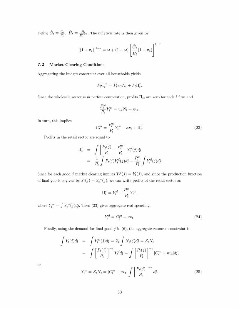
Define Gt ≡ GtP εt, Ht ≡ Ht

P ε−1t

. The inflation rate is then given by:

[(1 + πt)]1−ε = ω + (1− ω)

"Gt

Ht

(1 + πt)

#1−ε

7.2 Market Clearing Conditions

Aggregating the budget constraint over all households yields

PtCmt = PtwtNt + PtΠ

rt .

Since the wholesale sector is in perfect competition, profits Πit are zero for each i firm and

Pwt

PtY wt = wtNt + κvt.

In turn, this implies

Cmt =

Pwt

PtY wt − κvt +Π

rt . (23)

Profits in the retail sector are equal to

Πrt =

Z ∙Pt(j)

Pt− Pw

t

Pt

¸Y dt (j)dj

=1

Pt

ZPt(j)Y

dt (j)dj −

Pwt

Pt

ZY dt (j)dj

Since for each good j market clearing implies Y dt (j) = Yt(j), and since the production function

of final goods is given by Yt(j) = Y wt (j), we can write profits of the retail sector as

Πrt = Y dt −

Pwt

PtY wt ,

where Y wt =

RY wt (j)dj. Then (23) gives aggregate real spending:

Y dt = Cm

t + κvt. (24)

Finally, using the demand for final good j in (6), the aggregate resource constraint isZYt(j)dj =

ZY wt (j)dj = Zt

ZNt(j)dj = ZtNt

=

Z ∙Pt(j)

Pt

¸−εY dt dj =

Z ∙Pt(j)

Pt

¸−ε[Cm

t + κvt]dj,

or

Y wt = ZtNt = [C

mt + κvt]

Z ∙Pt(j)

Pt

¸−εdj. (25)

30

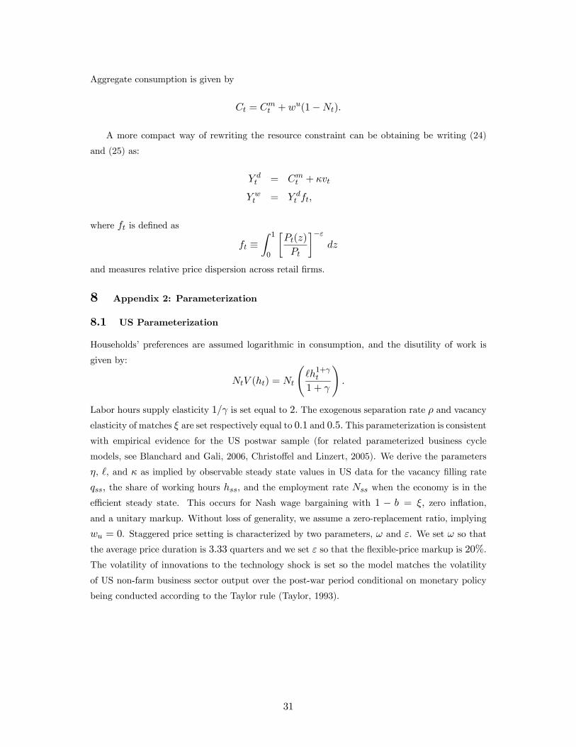
Aggregate consumption is given by

Ct = Cmt + wu(1−Nt).

A more compact way of rewriting the resource constraint can be obtaining be writing (24)

and (25) as:

Y dt = Cm

t + κvt

Y wt = Y d

t ft,

where ft is defined as

ft ≡Z 1

0

∙Pt(z)

Pt

¸−εdz

and measures relative price dispersion across retail firms.

8 Appendix 2: Parameterization

8.1 US Parameterization

Households’ preferences are assumed logarithmic in consumption, and the disutility of work is

given by:

NtV (ht) = Nt

Ãh1+γt

1 + γ

!.

Labor hours supply elasticity 1/γ is set equal to 2. The exogenous separation rate ρ and vacancy

elasticity of matches ξ are set respectively equal to 0.1 and 0.5. This parameterization is consistent

with empirical evidence for the US postwar sample (for related parameterized business cycle

models, see Blanchard and Gali, 2006, Christoffel and Linzert, 2005). We derive the parameters

η, , and κ as implied by observable steady state values in US data for the vacancy filling rate

qss, the share of working hours hss, and the employment rate Nss when the economy is in the

efficient steady state. This occurs for Nash wage bargaining with 1 − b = ξ, zero inflation,

and a unitary markup. Without loss of generality, we assume a zero-replacement ratio, implying

wu = 0. Staggered price setting is characterized by two parameters, ω and ε. We set ω so that

the average price duration is 3.33 quarters and we set ε so that the flexible-price markup is 20%.

The volatility of innovations to the technology shock is set so the model matches the volatility

of US non-farm business sector output over the post-war period conditional on monetary policy

being conducted according to the Taylor rule (Taylor, 1993).

31

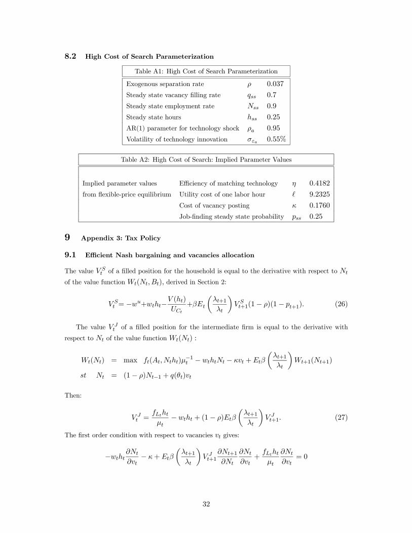
8.2 High Cost of Search Parameterization

Table A1: High Cost of Search Parameterization

Exogenous separation rate ρ 0.037

Steady state vacancy filling rate qss 0.7

Steady state employment rate Nss 0.9

Steady state hours hss 0.25

AR(1) parameter for technology shock ρa 0.95

Volatility of technology innovation σεa 0.55%

Table A2: High Cost of Search: Implied Parameter Values

Implied parameter values Efficiency of matching technology η 0.4182

from flexible-price equilibrium Utility cost of one labor hour 9.2325

Cost of vacancy posting κ 0.1760

Job-finding steady state probability pss 0.25

9 Appendix 3: Tax Policy

9.1 Efficient Nash bargaining and vacancies allocation

The value V St of a filled position for the household is equal to the derivative with respect to Nt

of the value function Wt(Nt, Bt), derived in Section 2:

V St = −wu+wtht−

V (ht)

UCt

+βEt

µλt+1λt

¶V St+1(1− ρ)(1− pt+1). (26)

The value V Jt of a filled position for the intermediate firm is equal to the derivative with

respect to Nt of the value function Wt(Nt) :

Wt(Nt) = max ft(At, Ntht)μ−1t − wthtNt − κvt +Etβ

µλt+1λt

¶Wt+1(Nt+1)

st Nt = (1− ρ)Nt−1 + q(θt)vt

Then:

V Jt =

fLthtμt− wtht + (1− ρ)Etβ

µλt+1λt

¶V Jt+1. (27)

The first order condition with respect to vacancies vt gives:

−wtht∂Nt

∂vt− κ+Etβ

µλt+1λt

¶V Jt+1

∂Nt+1

∂Nt

∂Nt

∂vt+

fLthtμt

∂Nt

∂vt= 0

32

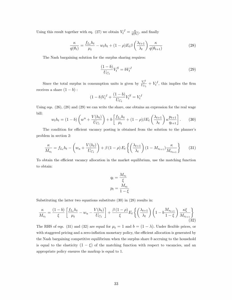
Using this result together with eq. (27) we obtain V Jt =

κq(θt)

, and finally

κ

q(θt)=

fLthtμt− wtht + (1− ρ)Etβ

µλt+1λt

¶κ

q(θt+1)(28)

The Nash bargaining solution for the surplus sharing requires:

(1− b)

UCt

V St = bV J

t (29)

Since the total surplus in consumption units is given by V St

UCt+ V J

t , this implies the firm

receives a share (1− b) :

(1− b)V Jt +

(1− b)

UCt

V St = V J

t

Using eqs. (26), (28) and (29) we can write the share, one obtains an expression for the real wage

bill:

wtht = (1− b)

µwu +

V (ht)

UCt

¶+ b

∙fLthtμt

+ (1− ρ)βEt

µλt+1λt

¶κpt+1qt+1

¸. (30)

The condition for efficient vacancy posting is obtained from the solution to the planner’s

problem in section 2:

κ

Mvt

= fLtht −µwu +

V (ht)

UCt

¶+ β (1− ρ)Et

½µλt+1λt

¶(1−Mst+1)

κ

Mvt+1

¾(31)

To obtain the efficient vacancy allocation in the market equilibrium, use the matching function

to obtain:

qt =Mvt

ξ

pt =Mst

1− ξ

Substituting the latter two equations substitute (30) in (28) results in:

κ

Mvt

=(1− b)

ξ

∙fLthtμt− wu −

V (ht)

UCt

¸+

β (1− ρ)

ξEt

½µλt+1λt

¶µ1− b

Mst+1

1− ξ

¶κξ

Mvt+1

¾(32)

The RHS of eqs. (31) and (32) are equal for μt = 1 and b = (1 − λ). Under flexible prices, or

with staggered pricing and a zero-inflation monetary policy, the efficient allocation is generated by

the Nash bargaining competitive equilibrium when the surplus share b accruing to the household

is equal to the elasticity (1 − ξ) of the matching function with respect to vacancies, and an

appropriate policy ensures the markup is equal to 1.

33

9.2 Tax policy enforcing the efficient allocation under Nash bargaining

Assume the intermediate firms’ revenues are taxed at the gross tax rate τ t. Then

V Jt =

κ

q(θt)= fLtht

µτ tμt

¶− wtht + (1− ρ)Etβ

µλt+1λt

¶κ

q(θt+1). (33)

Assume there exists a policy instrument τht affecting the households’ opportunity cost of having

an additional member in a match providing ht hours of work. We will later show that in the

efficient allocation τht 6= 1. From the perspective of the household, the value of a match is

V St ≡ wtht − τht

µwu +

V (ht)

UCt

¶+ βEt

µλt+1λt

¶V St+1(1− ρ)(1− pt+1) (34)

Using eqs. (33) and (34) the Nash-bargained wage is:

wtht = (1− b)τht

µwu +

V (ht)

UCt

¶+ b

∙fLtht

µτ tμt

¶+ (1− ρ)βEt

µλt+1λt

¶κpt+1qt+1

¸(35)

Substitute (35) in (33), using the equilibrium values of pt and qt. Equating the RHS of the

resulting equation with the RHS of eq. (31) gives:

(1− b)

ξ

∙fLtht

µτ tμt

¶− τht

µwu +

V (ht)

UCt

¶¸+(1− ρ)

ξβEt

µλt+1λt

¶µ1− b

Mst+1

1− ξ

¶κξ

Mvt+1

= fLtht −µwu +

V (ht)

UCt

¶+ β (1− ρ)Et

½µλt+1λt

¶(1−Mst+1)

κ

Mvt+1

¾For any b and τht , the equality is satisfied for:

τ tμt

=1

fLtht

∙τht (1− b)− ξ

(1− b)

¸µwu +

V (ht)

UCt

¶(36)

+ξ

(1− b)

½1− 1

fLthtβ (1− ρ)Et

∙µλt+1λt

¶µ1− b

1− ξ

¶Mst+1κ

Mvt+1

¸¾where

Mst+1

Mvt+1

= θt+1(1− ξ)

ξ

The tax τ t ensures that the first order condition for vacancy posting is identical to the planner’s

first order condition, that is, it corrects both for b 6= (1− ξ) and for the monopolistic distortion

μt 6= 1.

34

9.3 Tax policy enforcing the efficient allocation conditional on wage-setting

Divide both sides of eq. (33) by ξ, and equate the RHS to the RHS of (31):

ξ−1∙fLtht

µτ tμt

¶−wtht + (1− ρ)Etβ

µλt+1λt

¶κ

q(θt+1)

¸= fLtht −

µwu +

V (ht)

UCt

¶+ β (1− ρ)Et

½µλt+1λt

¶(1−Mst+1)

κ

Mvt+1

¾For any hourly wage wt, the equality is satisfied for:

τ tμt=

wt

fLt+

ξ

fLtht

∙fLtht −

µwu +

V (ht)

UCt

¶− β (1− ρ)Et

½µλt+1λt

¶Mst+1κ

Mvt+1

¾¸. (37)

Note that in this case τht does not appear in the tax policy condition, since the wage wt is taken

as given and V St is not used at any point in the derivation of eq. (37).

The tax (37) works by generating the correct surplus for the firm, conditional on all endogenous

variables being at their first best level. The firm receives a subsidy St per unit of output Y wt , or

per effective worker, equal to:

St =τ tfLtht

μt− fLtht

μt

= wtht + ξ

∙fLtht −

µwu +

V (ht)

UCt

¶− β (1− ρ)Et

½µλt+1λt

¶Mst+1κ

Mvt+1

¾¸− fLtht

μt

The firm’s surplus V ∗Jt is equal to the sum of the un-subsidized surplus V Jt obtained in eqs. (27),

(28) and the subsidy St, and can be rewritten as:

V ∗Jt =fLthtμt− wtht + (1− ρ)Etβ

µλt+1λt

¶κ

q(θt+1)+ St

= ξ

∙fLtht −

µwu +

V (ht)

UCt

¶− β (1− ρ)Et

½µλt+1λt

¶(1−Mst+1)

κ

Mvt+1

¾¸But this is equal to the firms’ surplus share ξ of the total surplus V ∗total in the efficient equilibrium

ξV ∗totalt

UCt

= ξ

∙fLtht −

µwu +

V (ht)

UCt

¶− β (1− ρ)Et

½µλt+1λt

¶(1−Mst+1)

κ

Mvt+1

¾¸This implies the subsidy St can be rewritten as

St = −V Jt + ξ

V ∗totalt

UCt

The intermediate tax τ t conditional on Nash bargaining is conceptually different from the

tax τ t conditional on a given wage process wt. This is more easily seen comparing a steady state

where agents agree on a fixed wage (a norm) equal to the Nash bargaining steady-state outcome

35

for a given b, and a steady state where agents agree to set the wage by Nash bargaining. If

the agents are Nash-bargaining, they agree on a rule to share the surplus. The total surplus

changes with τ t, so the steady state wage ends up being different from the steady state wage in

the absence of the surplus, conditional on b. For b > (1 − ξ) we have that τ > 1 in the steady

state. Under Nash-bargaining, the tax enforcing the first best will be higher than under a wage

norm. The wage also will be higher, though this is irrelevant for the allocation. All that is needed

for efficient vacancy posting is that the firm receives a share of the total surplus equal to ξ times

the surplus generated in the first best. The wage is only a transfer through the economy, and

any wage payment to the household in excess of the first-best wage is absorbed by the lump-sum

transfer to fund the intermediate firms’ subsidy.

9.4 Efficient hours choice

The intermediate tax τ t will generate the first best level of vacancy posting only conditional on

the choice of hours being efficient. As discussed in the main text, this can be achieved imposing

a tax τht affecting the households’ opportunity cost of work. Then the FOC for hours’ choice is

fLt

µτ tμt

¶=

µVhtUCt

¶τht (38)

and the optimal tax τht on households is

τht =τ tμt. (39)

Using eq. (39) to eliminate τht in eq. (36) we obtain

τ tμt=

ξ

(1− b)

(1− β (1− ρ)Et

∙µλt+1λt

¶µ1− b

1− ξ

¶Mst+1κ

Mvt+1

¸ ∙fLtht −

µwu +

V (ht)

UCt

¶¸−1).

9.5 Tax-equivalent policy

The tax-equivalent policy enforcing the intermediate sector tax τ tμt(36) or (37) is given by

1

μ∗t≡ τ t

μtμt = μ∗t

τht = 1

Whenever a tax policy scheme is not available, we assume a steady state subsidy to retail firms

τ rss ensures μss = 1, so that the Hosios condition holds when prices can be reset in every period,

or the monetary authority targets πt = 0.

36

9.6 Market clearing with tax policy

9.6.1 Household utility

To affect the household’s opportunity cost of work so that the disutility of working hours in eq.

(38) is given by³VhtUCt

´τht we assume the household has to supply (eτht − 1)ht hours of work

per employed worker to the government. These hours are transformed by the government in

utility-providing services Gt rebated to the household. 8 The household utility is then:

∪t = U(Ct)−NteV (ht) +GteV (ht) = V (eτht ht)

V (eτht ht) =(eτht ht)1+γ1 + γeτht = (τht )

11+γ

Gt =Nt (eτht ht)1+γ

1 + γ− Nt ht

1+γ

1 + γ

=Nt

h(eτht )1+γ − 1iht1+γ

1 + γ

This rebate scheme ensures thatVhtUCt

=³VhtUCt

´τht and at the same time the utility of the house-

hold is unaffected by the tax in the aggregate equilibrium. Therefore conditional on the first best

choices of Ct, Nt, ht the utility ∪t is also at the first best level.

9.6.2 Budget constraint

The derivation of eq. (34) and of the intermediate tax conditional on the Nash-bargained wage

assumes that the household pays a tax rate (τht −1) also on the home production of consumptiongoods wu(1−Nt). This assumption is made for analytical convenience, and is not central to any

of the results. All profits and taxes are rebated (or levied) lump-sum on the household’s. The

budget constraint can be written as:

PtCt + pbtBt+1 ≤ Pt[wthtNt + τhtwu(1−Nt)] +Bt + PtΠ

rt − Pt

hTht + Tt + T r

t

iT ht rebates to the household the tax τ

ht levied on wu(1−Nt) :

T ht = (τ

ht − 1)wu(1−Nt) (40)

Tt rebates to the household the tax τ t levied on the intermediate sector (or taxes the household

8For eτht < 1 the interpretation of the tax is identical, while the channels through which thehours’ exchange is transformed into utility for the household are reversed.

37

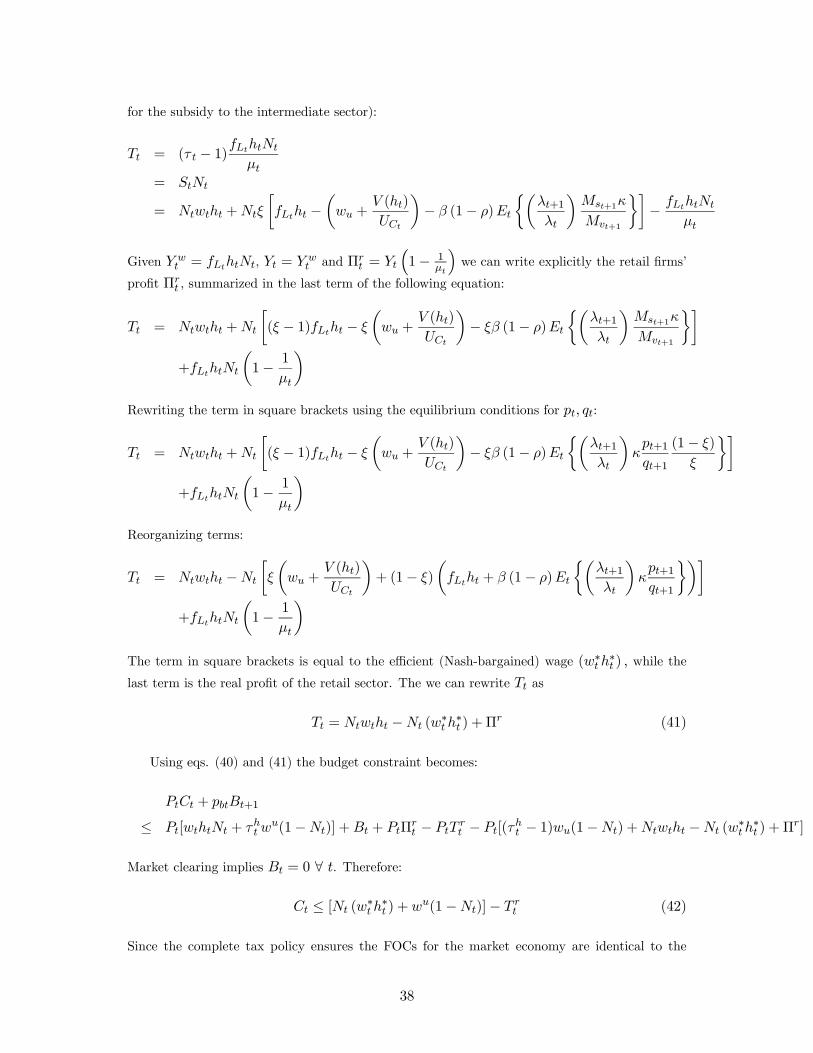
for the subsidy to the intermediate sector):

Tt = (τ t − 1)fLthtNt

μt= StNt

= Ntwtht +Ntξ

∙fLtht −

µwu +

V (ht)

UCt

¶− β (1− ρ)Et

½µλt+1λt

¶Mst+1κ

Mvt+1

¾¸− fLthtNt

μt

Given Y wt = fLthtNt, Yt = Y w

t and Πrt = Yt

³1− 1

μt

´we can write explicitly the retail firms’

profit Πrt , summarized in the last term of the following equation:

Tt = Ntwtht +Nt

∙(ξ − 1)fLtht − ξ

µwu +

V (ht)

UCt

¶− ξβ (1− ρ)Et

½µλt+1λt

¶Mst+1κ

Mvt+1

¾¸+fLthtNt

µ1− 1

μt

¶Rewriting the term in square brackets using the equilibrium conditions for pt, qt:

Tt = Ntwtht +Nt

∙(ξ − 1)fLtht − ξ

µwu +

V (ht)

UCt

¶− ξβ (1− ρ)Et

½µλt+1λt

¶κpt+1qt+1

(1− ξ)

ξ

¾¸+fLthtNt

µ1− 1

μt

¶Reorganizing terms:

Tt = Ntwtht −Nt

∙ξ

µwu +

V (ht)

UCt

¶+ (1− ξ)

µfLtht + β (1− ρ)Et

½µλt+1λt

¶κpt+1qt+1

¾¶¸+fLthtNt

µ1− 1

μt

¶The term in square brackets is equal to the efficient (Nash-bargained) wage (w∗t h

∗t ) , while the

last term is the real profit of the retail sector. The we can rewrite Tt as

Tt = Ntwtht −Nt (w∗t h∗t ) +Π

r (41)

Using eqs. (40) and (41) the budget constraint becomes:

PtCt + pbtBt+1

≤ Pt[wthtNt + τhtwu(1−Nt)] +Bt + PtΠ

rt − PtT

rt − Pt[(τ

ht − 1)wu(1−Nt) +Ntwtht −Nt (w

∗t h∗t ) +Π

r]

Market clearing implies Bt = 0 ∀ t. Therefore:

Ct ≤ [Nt (w∗t h∗t ) + wu(1−Nt)]− T r

t (42)

Since the complete tax policy ensures the FOCs for the market economy are identical to the

38

planner’s one, Nt and ht will be at their first-best level, and eq. (42) implies the consumption

level Ct will also attain its efficient level for T rt = 0.

The tax T rt is nonzero only when the tax instruments τ t and τ

ht are not available, and funds

the transfer to the retail firms ensuring that in a zero-inflation equilibrium the markup μ is equal

to 1. This allows the market allocation to be efficient if πt = 0 ∀ t , wages are Nash-bargainedand the Hosios condition b = (1−ξ) is met. The net subsidy to retail firms is equal to (1−τ rss)Ytand τ rss = μ = ε

ε−1 . In a zero-inflation equilibrium

Pwt

Pt=

τ rssμ

The optimal gross subsidy per unit of output is

τ rss = μ

The retail sector total profits are given by

Πrt = τ rssYt −τ rssμYt

= (μ− 1)Yt

Therefore the tax on the household sector is equal to:

T rt = (μ− 1)Yt

39

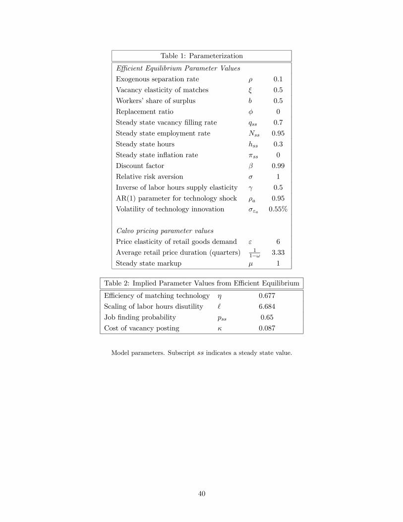
Table 1: Parameterization

Efficient Equilibrium Parameter Values

Exogenous separation rate ρ 0.1

Vacancy elasticity of matches ξ 0.5

Workers’ share of surplus b 0.5

Replacement ratio φ 0

Steady state vacancy filling rate qss 0.7

Steady state employment rate Nss 0.95

Steady state hours hss 0.3

Steady state inflation rate πss 0

Discount factor β 0.99

Relative risk aversion σ 1

Inverse of labor hours supply elasticity γ 0.5

AR(1) parameter for technology shock ρa 0.95

Volatility of technology innovation σεa 0.55%

Calvo pricing parameter values

Price elasticity of retail goods demand ε 6

Average retail price duration (quarters) 11−ω 3.33

Steady state markup μ 1

Table 2: Implied Parameter Values from Efficient Equilibrium

Efficiency of matching technology η 0.677

Scaling of labor hours disutility 6.684

Job finding probability pss 0.65

Cost of vacancy posting κ 0.087

Model parameters. Subscript ss indicates a steady state value.

40

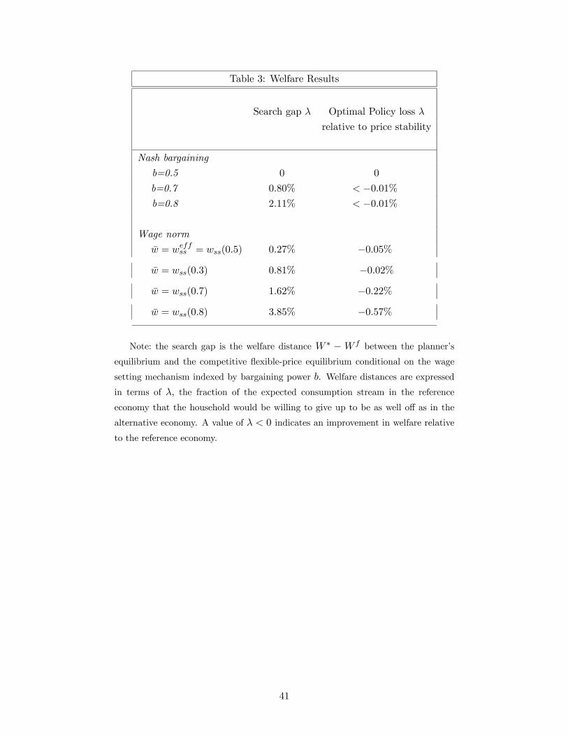
Table 3: Welfare Results

Search gap λ Optimal Policy loss λ

relative to price stability

Nash bargaining

b=0.5 0 0

b=0.7 0.80% < −0.01%b=0.8 2.11% < −0.01%

Wage norm

w = weffss = wss(0.5) 0.27% −0.05%

w = wss(0.3) 0.81% −0.02%

w = wss(0.7) 1.62% −0.22%

w = wss(0.8) 3.85% −0.57%

Note: the search gap is the welfare distance W ∗ −W f between the planner’s

equilibrium and the competitive flexible-price equilibrium conditional on the wage

setting mechanism indexed by bargaining power b. Welfare distances are expressed

in terms of λ, the fraction of the expected consumption stream in the reference

economy that the household would be willing to give up to be as well off as in the

alternative economy. A value of λ < 0 indicates an improvement in welfare relative

to the reference economy.

41

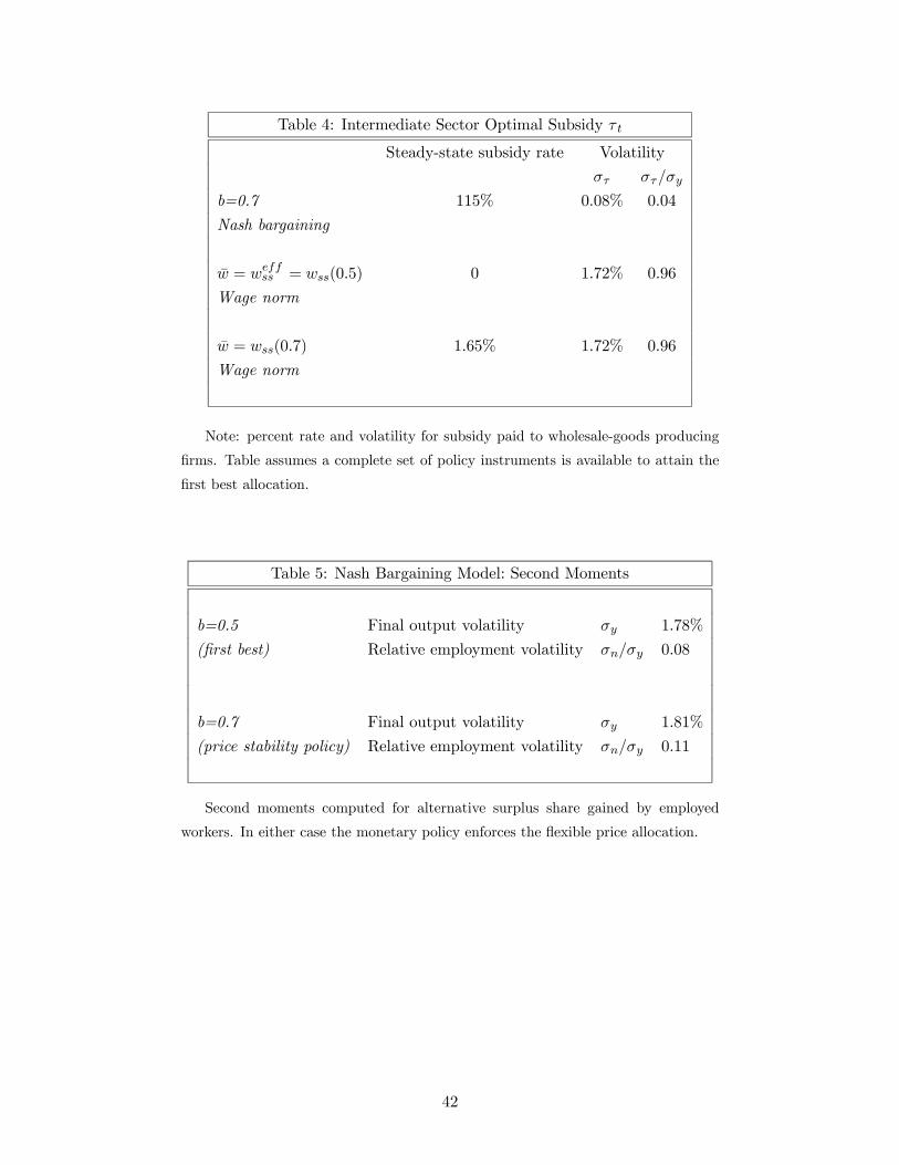
Table 4: Intermediate Sector Optimal Subsidy τ t

Steady-state subsidy rate Volatility

στ στ/σy

b=0.7 115% 0.08% 0.04

Nash bargaining

w = weffss = wss(0.5) 0 1.72% 0.96

Wage norm

w = wss(0.7) 1.65% 1.72% 0.96

Wage norm

Note: percent rate and volatility for subsidy paid to wholesale-goods producing

firms. Table assumes a complete set of policy instruments is available to attain the

first best allocation.

Table 5: Nash Bargaining Model: Second Moments

b=0.5 Final output volatility σy 1.78%

(first best) Relative employment volatility σn/σy 0.08

b=0.7 Final output volatility σy 1.81%

(price stability policy) Relative employment volatility σn/σy 0.11

Second moments computed for alternative surplus share gained by employed

workers. In either case the monetary policy enforces the flexible price allocation.

42

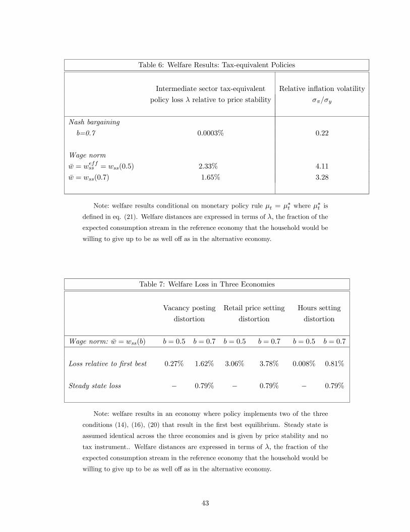
Table 6: Welfare Results: Tax-equivalent Policies

Intermediate sector tax-equivalent Relative inflation volatility

policy loss λ relative to price stability σπ/σy

Nash bargaining

b=0.7 0.0003% 0.22

Wage norm

w = weffss = wss(0.5) 2.33% 4.11

w = wss(0.7) 1.65% 3.28

Note: welfare results conditional on monetary policy rule μt = μ∗t where μ∗t is

defined in eq. (21). Welfare distances are expressed in terms of λ, the fraction of the

expected consumption stream in the reference economy that the household would be

willing to give up to be as well off as in the alternative economy.

Table 7: Welfare Loss in Three Economies

Vacancy posting Retail price setting Hours setting

distortion distortion distortion

Wage norm: w = wss(b) b = 0.5 b = 0.7 b = 0.5 b = 0.7 b = 0.5 b = 0.7

Loss relative to first best 0.27% 1.62% 3.06% 3.78% 0.008% 0.81%

Steady state loss − 0.79% − 0.79% − 0.79%

Note: welfare results in an economy where policy implements two of the three

conditions (14), (16), (20) that result in the first best equilibrium. Steady state is

assumed identical across the three economies and is given by price stability and no

tax instrument.. Welfare distances are expressed in terms of λ, the fraction of the

expected consumption stream in the reference economy that the household would be

willing to give up to be as well off as in the alternative economy.

43

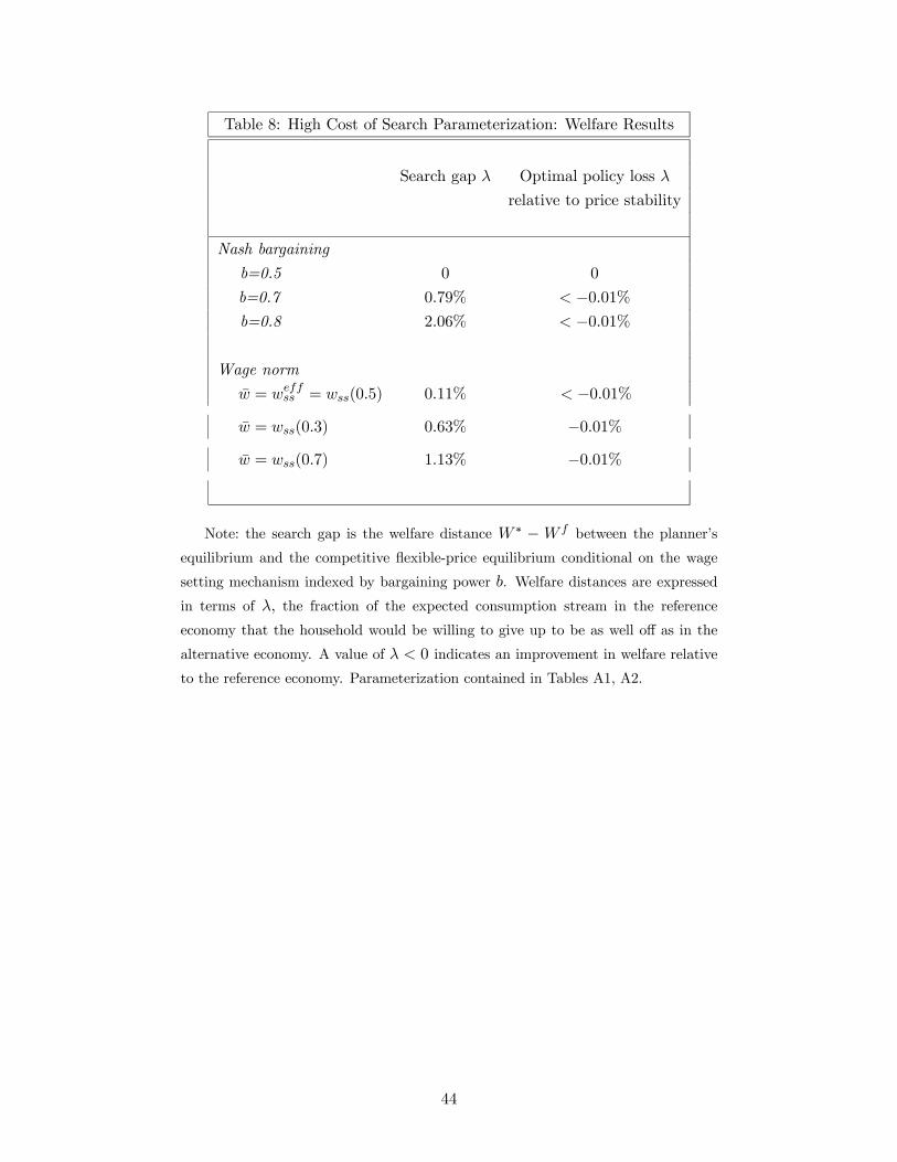
Table 8: High Cost of Search Parameterization: Welfare Results

Search gap λ Optimal policy loss λ

relative to price stability

Nash bargaining

b=0.5 0 0

b=0.7 0.79% < −0.01%b=0.8 2.06% < −0.01%

Wage norm

w = weffss = wss(0.5) 0.11% < −0.01%

w = wss(0.3) 0.63% −0.01%

w = wss(0.7) 1.13% −0.01%

Note: the search gap is the welfare distance W ∗ −W f between the planner’s

equilibrium and the competitive flexible-price equilibrium conditional on the wage

setting mechanism indexed by bargaining power b. Welfare distances are expressed

in terms of λ, the fraction of the expected consumption stream in the reference

economy that the household would be willing to give up to be as well off as in the

alternative economy. A value of λ < 0 indicates an improvement in welfare relative

to the reference economy. Parameterization contained in Tables A1, A2.

44

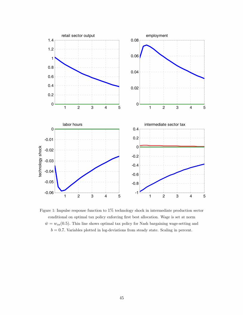
1 2 3 4 50

0.2

0.4

0.6

0.8

1

1.2

1.4retail sector output

1 2 3 4 50

0.02

0.04

0.06

0.08employment

1 2 3 4 5-0.06

-0.05

-0.04

-0.03

-0.02

-0.01

0labor hours

tech

nolo

gy s

hock

1 2 3 4 5-1

-0.8

-0.6

-0.4

-0.2

0

0.2

0.4intermediate sector tax

Figure 1: Impulse response function to 1% technology shock in intermediate production sector

conditional on optimal tax policy enforcing first best allocation. Wage is set at norm

w = wss(0.5). Thin line shows optimal tax policy for Nash bargaining wage-setting and

b = 0.7. Variables plotted in log-deviations from steady state. Scaling in percent.

45

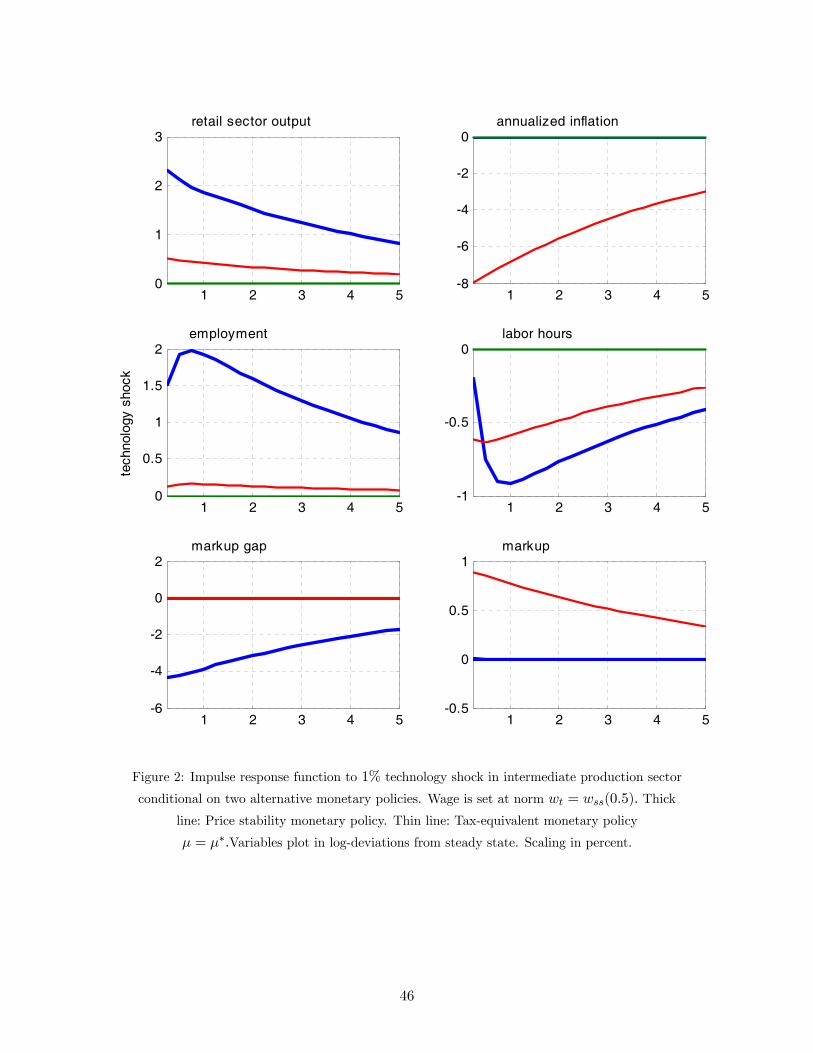
1 2 3 4 50

1

2

3retail sector output

1 2 3 4 5-8

-6

-4

-2

0annualized inflation

1 2 3 4 50

0.5

1

1.5

2employment

tech

nolo

gy s

hock

1 2 3 4 5-1

-0.5

0labor hours

1 2 3 4 5-6

-4

-2

0

2markup gap

1 2 3 4 5-0.5

0

0.5

1markup

Figure 2: Impulse response function to 1% technology shock in intermediate production sector

conditional on two alternative monetary policies. Wage is set at norm wt = wss(0.5). Thick

line: Price stability monetary policy. Thin line: Tax-equivalent monetary policy

μ = μ∗.Variables plot in log-deviations from steady state. Scaling in percent.

46

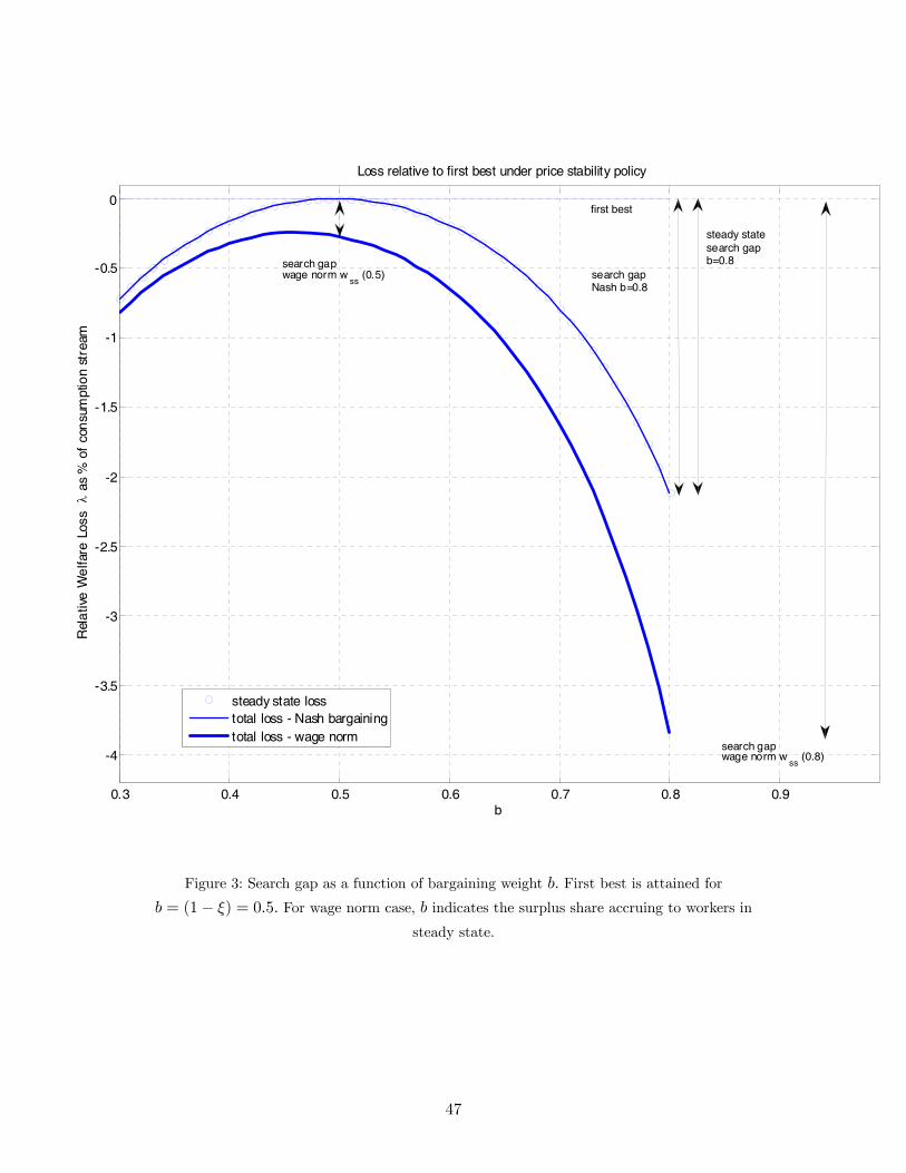
0.3 0.4 0.5 0.6 0.7 0.8 0.9

-4

-3.5

-3

-2.5

-2

-1.5

-1

-0.5

0

b

Rel

ativ

e W

elfa

re L

oss

λ a

s %

of

con

sum

ptio

n st

ream

Loss relative to first best under price stability policy

first best

steady state search gap b=0.8

search gap wage norm w

ss (0.8)

search gap wage norm w

ss (0.5)

steady state losstotal loss - Nash bargainingtotal loss - wage norm

search gap Nash b=0.8

Figure 3: Search gap as a function of bargaining weight b. First best is attained for

b = (1− ξ) = 0.5. For wage norm case, b indicates the surplus share accruing to workers in

steady state.

47