Monetary and Fiscal Policy Interaction: The Consequences ...aei.pitt.edu/33072/1/jones._jason_cannon.pdf · Monetary and Fiscal Policy Interaction: ... Monetary and Fiscal Policy

1

Monetary and Fiscal Policy Interaction: The Consequences of Joining a

Monetary Union.

Jason Jones

Furman University

[email protected]

April 2009

The great experiment in monetary unification across Europe is just beginning to provide the data

needed to test the theories and debates surrounding the costs and benefits of forming a union. This

paper will explore one particular aspect of the unification process, the effect it had on monetary and

fiscal strategic interaction. Using a panel structural VAR to measure monetary and fiscal policy

interaction among EMU members before and after joining the EMU, a difference in this interaction is

detected. Pre‐EMU the monetary and fiscal authority acted as strategic substitutes in the case of a

monetary response to a fiscal receipts shock (such as a discretionary increase in taxes). After the

formation of the union this relationship disappears and there is no strategic interaction. The timing of

the change suggests a role for the Maastricht treaty coupled with the weak SGP.

Draft:

Presented in the EUSA Conference 2009: Los Angeles

April 23‐25, 2009

Please do not quote

2

Monetary and Fiscal Policy Interaction: The Consequences of Joining a

Monetary Union.

1. Introduction

The great experiment in monetary unification across Europe is just beginning to provide the data

needed to test the theories and debates surrounding the costs and benefits of forming a union. Studying

the actual costs and benefits of a monetary union the size of the EMU will help deter or accelerate the

expansion of the current EMU, as well as the possible formation of other monetary unions across the

world. At the very least the EMU experience provides information on how countries who do decide to

form a monetary union can prepare for the issues that arise.

This paper will explore one particular aspect of the unification process, the effect it had on

monetary and fiscal strategic interaction. The process and effects of monetary policy (to a greater

extent) and fiscal policy (to a lesser extent) on macroeconomic variables such as output and inflation

have been extensively studied.1 The characteristics of the interaction between these policy makers,

however, have received less attention in general and even less in relation to the monetary union

(Muscatelli, Tirelli, and Trecroci, 2004). Policy makers interact as strategic substitutes when one policy

maker’s decision to conduct expansionary (contractionary) policy is met with contractionary

(expansionary) policy by the other. For example, if the monetary authority were to raise interest rates

the fiscal authority would respond by either increasing spending or lowering taxes. If they act as

strategic complements expansionary policy by one authority is met with expansionary policy by the

other and vice versa.

There are features specific to monetary unions as well as the European Monetary Union (EMU)

1 See Christiano, Eichenbaum, and Even (1999) for a summary of monetary policy empirical research and Caldara

and Kamps (2008) for a summary of fiscal policy empirical research.

3

that suggest the relationship between monetary and fiscal authorities may change as a result of

becoming a member. One salient feature of becoming a member of a monetary union is the loss of the

ability to conduct independent monetary policy. The fiscal and monetary authority previous to joining

the union function within the same national boundaries, interacting one with another in response to

common economic fluctuations. After the formation of the union (in the absence of a central fiscal

authority, as is the case in the EMU), the fiscal authority maintains its focus on the country specific

needs while the monetary authority reacts to aggregate economic fluctuations. The greater “distance”

not only in terms of physicality but purpose as well, could fundamentally change the way in which policy

makers strategically interact.

In the case of the EMU it is also important to take into account the external restrictions placed

on the conduct of monetary and fiscal policy in the run up to the creation of the monetary union and

beyond. In order to insure that countries met the optimal currency criteria as introduced by Mundell

(1961), potential members were required to meet certain convergence criteria. These were spelled out

in the Maastricht Treaty signed in 1992. Members were to maintain exchange rates within a specified

band, bring inflation to within 1.5 percentage points of the lowest inflation members, bring nominal

long‐term interest rates to within 2 percentage points of the low inflation countries, and bring budget

deficits to within 3 percent of GDP and the national debt to 60 percent of GDP (Afxentiou, 2000).

Meeting these criteria restricted the conduct of stabilizing fiscal policy for most members as they almost

all had to reduce their budget deficits. It also forced monetary authorities of many potential members to

concentrate primarily on inflation reduction, as many members had to lower inflation in order to meet

the criteria. These restrictions and the role each policy maker played in order to meet the criteria could

change the nature of interaction between policy makers (Leith and Wren‐Lewis, 2000). The deficit

restrictions were maintained under the Stability and Growth Pact (SGP) after the formation of the union

and continue to restrict the conduct of fiscal policy if a member finds itself near the threshold in times of

4

economic trouble. The SGP has turned out to be less effective in restricting deficits, as a number of

members violated the deficit threshold within the first five years of the union. As a result, the effects of

fiscal restriction on interaction may be less so post‐EMU.

Structural VARs using short run restriction are used to estimate monetary and fiscal interaction

and compare them over the process of monetary unification in Europe. The estimation reveals that

monetary and fiscal interaction did change after the advent of the monetary union in terms of how

monetary authorities respond to revenue policy conducted by the government. Pre‐EMU the policy

makers acted as strategic substitutes while after the formation of the union there is no significant

interaction. Though the causes of this observation are not fully explored, the results suggest the

Maastricht convergence criteria played an important role.

In Section two theoretical and empirical studies of monetary and fiscal interaction are reviewed.

In Section three the empirical model used to estimate monetary and fiscal interaction in Europe is

introduced and estimated. Section four finishes with a discussion of the results as well as needed

extension.

2. Monetary and Fiscal strategic interaction

2.1 Theoretical

The creation of the EMU led to a number of studies that set out to model the potential difficulties

associated with monetary and fiscal policy in a monetary union. Great attention was paid to modeling

how fiscal restrictions under the SGP would affect this relationship. Governatori and Eijffinger (2004),

and Buti, Roeger, and In’t Veld (2001) use a game theoretic approaches to analyze how the strategic

relationship between independent fiscal authorities and a common monetary authority. Governatroi

and Eijffinger (2004) illustrate the free rider problem that exists in fiscal policy conducted in a monetary

5

union. They show how the SGP does help to internalize the negative effects of deficit spillovers but the

restriction is not enough to trigger the first best equilibrium of no deficits, no output gap, and stable

inflation. Buti, Roeger, and In’t Veld (2001) model the circumstances leading to fiscal coordination

among monetary members. They find that substitutability and complementarity between policies

depends on the type of shock hitting the economy. When fiscal authorities do not coordinate the

central bank prefers high fiscal stabilization in the face of demand shocks and low in the face of supply

shocks. Gains to co‐operation are low when dealing with demand shocks but higher when there are

supply shocks. They also show that expansionary fiscal policy leads to monetary tightening in this one

country case.

Model simulations are also used to discuss interaction between monetary and fiscal policy

makers in a monetary union. Leith and Wren‐Lewis (2000) simulate a perpetual‐youth model of a

member of a monetary union to address the usefulness of budgetary restriction in a monetary union.

They find that when the fiscal authority is constrained to stabilize its debt, the monetary authority is free

to conduct its policy. On the other hand, if the fiscal authority is not self‐stabilizing the monetary

authority may have to reduce real interest rates when there is excess inflation. This finding justifies fiscal

rules, though they do note that the SGP is more stringent than is needed. Van Aarle, Gerretsen, and

Huart (2004) look at the effects on having different monetary and fiscal rules in the EMU. They use

simulations from a calibrated two country New Neoclassical New Keynesian dynamic model. The mode

consists of an IS curve for each country as well as a hybrid Phillips curve for each country. There is one

central bank which follows a Taylor rule while the fiscal authorities follow individual “fiscal Taylor rules”.

In their model of members of a monetary union they find strategic substitution. If there is a supply shock

the monetary authority increases interest rates while the fiscal authorities of each country conduct

expansionary policy to close the output gap. In the case of demand shock the monetary authority and

each fiscal authority work together. In response to a country specific fiscal shock, say a reduction in the

6

deficit, a neighboring country must increase its deficit to combat the spillover effects that come as a

result of trade. In this case however the common monetary authority helps in that it conducts

expansionary policy in response the original country’s restrictive policy.

Their simulation of a two country model suggests that in response to a monetary shock deficits

will increase; the policy makers act as strategic substitutes. The two authorities also act as strategic

substitutes in the face of a fiscal shock.

Advanced DSGE models have also been created that allow for strategic interaction between

monetary and fiscal authorities. Benigno and Woodford (2003) demonstrate that a dynamic macro‐

foundations model can be constructed that allows for both the monetary and fiscal authority to respond

optimally to fluctuations in the economy. Their results indicate that the monetary and fiscal authority

should take into account how the actions they perform influence the goals of the other policy maker.

Gali and Monacelli (2005) created a monetary union DSGE model were monetary and fiscal authorities

both choosing their policy optimally. They show that under optimal policy, inflation is stabilized at the

union level but there remains a stabilization role for fiscal policy. Fiscal stabilization is desirable not only

for the individual country but the union as a whole if it is coordinated among members. When there is

no fiscal coordination the policy makers’ actions lead to a suboptimal outcome, where the common

central bank faces a trade‐off between inflation and output gap stabilization at the union level.

2.2 Empirical

The interaction between monetary and fiscal authorities has been empirically measured in a number of

different ways. Most studies estimate fiscal response functions that include a measure of monetary

policy. Melitz (1997) estimated a pooled data set of 19 OECD countries (including 14 EU members) and

finds that monetary and fiscal policy makers act as strategic substitutes. In response to a monetary

tightening, fiscal policy would expand or not tighten as much as the monetary tightening. Von Hagen,

7

Hughes Hallet, and Strauch (2000) use a panel of 20 OECD countries from 1973 to 1989 to study fiscal

consolidations. They find that when monetary policy is relaxed fiscal policy responds as a strategic

substitute, but when fiscal policy is tightened the monetary authority responds as a strategic

complement. When they limit the sample to European countries they do find a `Maastricht effect’,

where in the 1990s fiscal policy becomes less reactive to monetary policy than before (as well as to

cyclical fluctuations).

Gali and Perotti (2003) and the IMF (2004) estimate fiscal reaction functions for the EMU

members using two stage least squares for individual countries as well as panel data. Gali and Perotti

use data from 1980 to 2002 while the IMF uses data from 1971 to 2004. Both find that in general EU

members’ fiscal and monetary policy makers have acted as substitutes, though the magnitude is small.

Both studies attempt to estimate changes to this relationship as a result of joining the union using

dummy variables. They find that though there is no statistical difference in the reactions pre‐ and post‐

EMU in their small sample the response is smaller post‐EMU. Claeys (2006) also estimates a fiscal

reaction function with an instrumental variable GMM approach. He uses seven EU countries and finds

significant strategic substitution only in Germany for data up to 2003, though he does suggest that a

monetary union could lead to greater fiscal activism. There is no attempt to estimate differences as a

result of joining the union however.

Estimation of single equation fiscal reaction functions do provide information and while

instruments do take into account the endogeneity of the output gap, there is still the possibility of

simultaneous equation bias. Every variable of interest is determined by the other. A single equation

representation of a fiscal rule alone does not allow for a simultaneous measure of how monetary policy

may strategically react to fiscal disturbances, nor would the estimation of a monetary rule allow for a

measure of fiscal reaction to monetary movements.

8

Favero (2002) begins to address this issue using seemingly unrelated regression. In his

estimation however there is no direct measure of strategic interaction between the fiscal and monetary

authorities. Structural VARs (SVAR), as will be explained below, are well suited for this type of problem

as long as the structural shocks can be confidently identified. Using SVARs allow for the inclusion of

both monetary and fiscal policies, and thus measure strategic interaction between policy makers. There

are a number of competing methods in using SVARs to identify fiscal shocks and thus monetary

reactions to them. This paper will follow Fatas and Mihov’s (2001) recursive approach coupled with

Blanchard and Perotti’s (2002) identification approach which takes into account automatic stabilizers.

Other methods of fiscal and monetary shock identification use SVARs, such as Mountford and

Uhlig (2005) who use sign restrictions to identify structural shocks. Ramey and Shapiro (1998) introduce

an events method, essentially identifying fiscal shocks in US history and using those points in time as

dummy to model fiscal shocks. Caldara and Kamps (2008) compare and contrast each of these

estimation techniques using US data. They find that even though there are some differences across

models in how wages and consumption respond to fiscal shocks, they are all consistent in predicting

strategic policy interaction for the US. Monetary policy makers do not respond to spending shocks, but

the act as strategic substitutes in the case of a tax shock.2

The narrative approach is limited in its use because it requires a list of significant spending and

taxing shocks and such a list has not yet been compiled for the European nations. The use of sign

restrictions have received less attention and seems to provide little advantage over other methods in

regards to the question at hand. This paper thus will use a recursive SVAR to measure monetary and

fiscal reactions using pre‐ and post‐EMU data. Impulse response functions are then estimated and

2 The narrative (events) approach did not allow for a measure of how monetary policy reacts to a tax shock as

Ramey and Shapiro (1998) only identify spending shocks in United States historical data.

9

compared pre‐ and post‐EMU using a Wald test. Any significant differences would indicate a change in

strategic behavior between monetary and fiscal authorities as a result of joining the monetary union.

3. Testing the Nature of Responses

3.1 Estimation Techniques

In order to examine monetary and fiscal interaction, their respective reaction functions need to be

estimated. It is assumed that fiscal and monetary authorities respond to inflation and output

fluctuations, yet their actions are not independent. For example a dynamic fiscal spending (s) reaction

function could include output (y), inflation (π), government receipts (r), or the monetary reaction (i), as

well as its own lag and the lags of the other variables:

sttttttttttt viyrsiyrs ...1

1151

1141

1131

1121

111

015

014

013

012

Yet receipts also respond to spending, output, inflation, the interest rate, and its lag as well as the lags

of the other variables:

rttttttttttt viysriysr ...1

1251

1241

1231

1211

122

025

024

023

021

The monetary response would react to the same variables as well. In addition, output and inflation

would be influenced by fiscal and monetary movements. Thus an OLS estimation of each of these

relationships independent of one another would be biased because of simultaneity. Using VAR these

relationships can be estimated as a system. Restrictions on the errors of the reduced form VAR allow for

consistent estimates of the structural parameters of the model, specifically the structural error terms.

Thus the SVAR (a reduced form VAR with identifying restrictions imposed) can be used to identify

structural fiscal and monetary shocks and the reaction to them by the other variables in the VAR. The

simultaneous system of equations can be collected and written in vector form as:

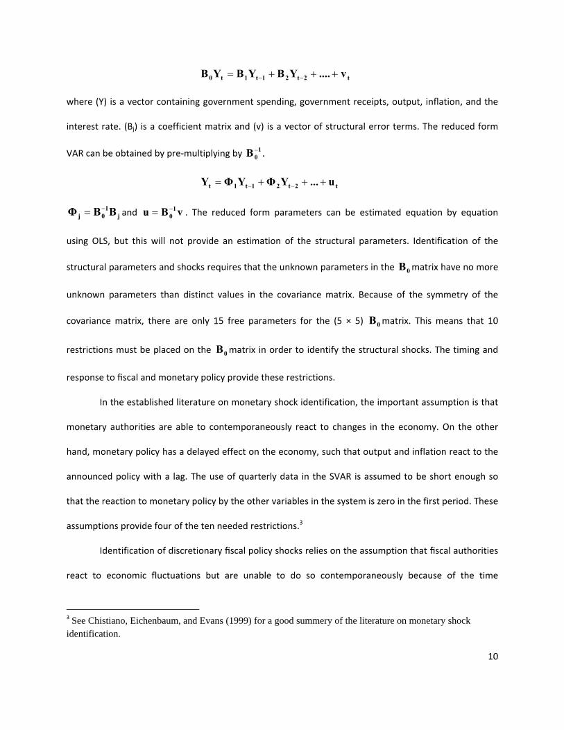
10

t2t21t1t0 v....YBYBYB

where (Y) is a vector containing government spending, government receipts, output, inflation, and the

interest rate. (Bj) is a coefficient matrix and (v) is a vector of structural error terms. The reduced form

VAR can be obtained by pre‐multiplying by .10B

t2t21t1t u...YΦYΦY

j10j BBΦ and vBu 1

0 . The reduced form parameters can be estimated equation by equation

using OLS, but this will not provide an estimation of the structural parameters. Identification of the

structural parameters and shocks requires that the unknown parameters in the 0B matrix have no more

unknown parameters than distinct values in the covariance matrix. Because of the symmetry of the

covariance matrix, there are only 15 free parameters for the (5 × 5) 0B matrix. This means that 10

restrictions must be placed on the 0B matrix in order to identify the structural shocks. The timing and

response to fiscal and monetary policy provide these restrictions.

In the established literature on monetary shock identification, the important assumption is that

monetary authorities are able to contemporaneously react to changes in the economy. On the other

hand, monetary policy has a delayed effect on the economy, such that output and inflation react to the

announced policy with a lag. The use of quarterly data in the SVAR is assumed to be short enough so

that the reaction to monetary policy by the other variables in the system is zero in the first period. These

assumptions provide four of the ten needed restrictions.3

Identification of discretionary fiscal policy shocks relies on the assumption that fiscal authorities

react to economic fluctuations but are unable to do so contemporaneously because of the time

3 See Chistiano, Eichenbaum, and Evans (1999) for a good summery of the literature on monetary shock identification.

11

necessary to draft and approve changes to spending or taxes. Fatas and Mihov (2001) use a recursive

approach to identify fiscal shocks. Blanchard and Perotti (2002) extend this work of fiscal shock

identification by using timing restrictions in a SVAR while taking into account automatic stabilizers.

Perotti (2002) and Canzoneri, Cumby, and Diba (2002) have expanded on Blanchard and Perotti’s

technique by including monetary policy as well as a number of other variables.

Fatas and Mihov as well as Blanchard and Perotti, use government spending and tax revenue

(net of transfers) as arguments in their SVAR. These series respond within the quarter to movements in

output through both automatic stabilizers and discretionary fiscal policy. Blanchard and Perotti remove

the cyclical component from the reduced form residuals using outside estimations of the output

elasticity of government spending and tax revenue found in Giorno, Richardson, Roseveare, and van der

Noord (1995). Perotti (2002) expands the VAR to include inflation and monetary interaction, in which

case he also estimates and uses the inflation elasticity of government spending and tax revenue. These

estimations allow them to construct a cyclically adjusted government spending and tax revenue residual

and provide two more restrictions on the SVAR. It is also assumed that government spending and

receipts do affect output, inflation, and monetary policy within a quarter but are unable to respond to

output, inflation, and the interest rate within one quarter because of the legislative inside lag. It is also

assumed that spending does not respond within the quarter to changes in output. They take an agnostic

stance on whether taxes affect spending, or spending effects taxes within the quarter, yet to get the

final needed identification restriction receipts are assumed to not respond to spending within the

quarter, while spending does respond to receipts.4 These assumptions provide the remaining four

restrictions needed to identify the structural parameters. As a result the relationship between structural

disturbances (vt) and the reduced form disturbances (ut) is represented by:

4 This ordering assumption is reversed and found to not cause any significant change in the results.

12

itti

ytiy

rtir

stis

it

tyty

rtr

stst

yt

rtyr

stys

yt

rt

strstr

ytry

rt

stts

st

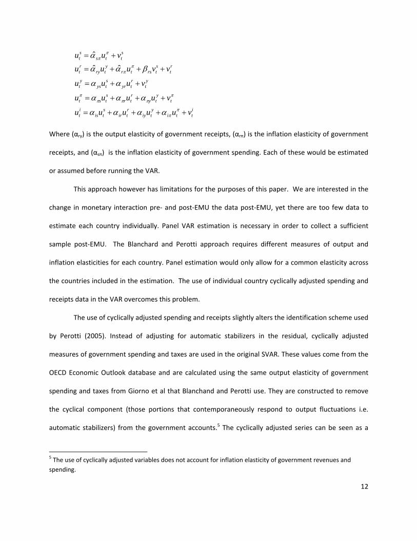
vuuuuu

vuuuu

vuuu

vvuuu

vuu

ˆˆ

ˆ

Where (αry) is the output elasticity of government receipts, (αrπ) is the inflation elasticity of government

receipts, and (αsπ) is the inflation elasticity of government spending. Each of these would be estimated

or assumed before running the VAR.

This approach however has limitations for the purposes of this paper. We are interested in the

change in monetary interaction pre‐ and post‐EMU the data post‐EMU, yet there are too few data to

estimate each country individually. Panel VAR estimation is necessary in order to collect a sufficient

sample post‐EMU. The Blanchard and Perotti approach requires different measures of output and

inflation elasticities for each country. Panel estimation would only allow for a common elasticity across

the countries included in the estimation. The use of individual country cyclically adjusted spending and

receipts data in the VAR overcomes this problem.

The use of cyclically adjusted spending and receipts slightly alters the identification scheme used

by Perotti (2005). Instead of adjusting for automatic stabilizers in the residual, cyclically adjusted

measures of government spending and taxes are used in the original SVAR. These values come from the

OECD Economic Outlook database and are calculated using the same output elasticity of government

spending and taxes from Giorno et al that Blanchand and Perotti use. They are constructed to remove

the cyclical component (those portions that contemporaneously respond to output fluctuations i.e.

automatic stabilizers) from the government accounts.5 The cyclically adjusted series can be seen as a

5 The use of cyclically adjusted variables does not account for inflation elasticity of government revenues and

spending.

13

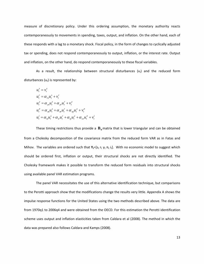
measure of discretionary policy. Under this ordering assumption, the monetary authority reacts

contemporaneously to movements in spending, taxes, output, and inflation. On the other hand, each of

these responds with a lag to a monetary shock. Fiscal policy, in the form of changes to cyclically adjusted

tax or spending, does not respond contemporaneously to output, inflation, or the interest rate. Output

and inflation, on the other hand, do respond contemporaneously to these fiscal variables.

As a result, the relationship between structural disturbances (vt) and the reduced form

disturbances (ut) is represented by:

itti

ytiy

rtir

stis

it

tyty

rtr

stst

yt

rtyr

stys

yt

rt

strs

rt

st

st

vuuuuu

vuuuu

vuuu

vuu

vu

These timing restrictions thus provide a 0B matrix that is lower triangular and can be obtained

from a Cholesky decomposition of the covariance matrix from the reduced form VAR as in Fatas and

Mihov. The variables are ordered such that Yt=[st rt yt πt it]. With no economic model to suggest which

should be ordered first, inflation or output, their structural shocks are not directly identified. The

Cholesky framework makes it possible to transform the reduced form residuals into structural shocks

using available panel VAR estimation programs.

The panel VAR necessitates the use of this alternative identification technique, but comparisons

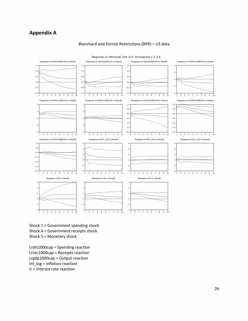
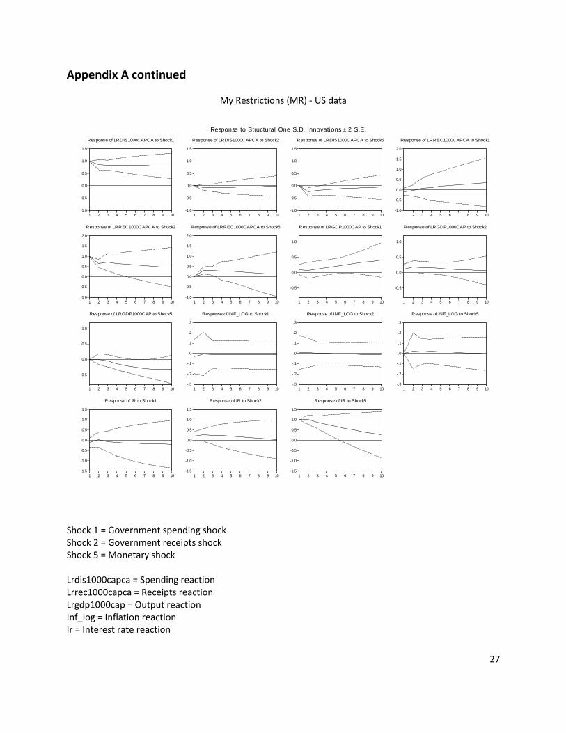
to the Perotti approach show that the modifications change the results very little. Appendix A shows the

impulse response functions for the United States using the two methods described above. The data are

from 1970q1 to 2006q4 and were obtained from the OECD. For this estimation the Perotti identification

scheme uses output and inflation elasticities taken from Caldara et al (2008). The method in which the

data was prepared also follows Caldara and Kamps (2008).

14

The responses and significance of the responses are similar across the two estimation

techniques. The point of biggest departure in terms of direction and significance is in the response of

inflation to a spending shock. This is not as surprising as cyclically adjusted variables do not take into

account the price elasticity of spending while Blanchard and Perotti do. In terms of precision, the

Blanchard and Perotti approach does find slight significant responses in the initial period following a

shock for a spending response to a receipt shock, an output response to a receipt shock, and an interest

rate response to a receipt shock, where my method does not. Only in one case, a receipt response to a

monetary shock, does my method provide a significant response where the Perotti approach did not and

only by a small margin. In each of these cases the response is of similar shape and direction. In two

cases, a receipt response to a spending shock and an output response to a spending shock, do the

modes differ in estimated directions, but in both of these cases the response is insignificant. As my

method appears to correctly identify the shape and direction of response in relation to the Perotti

approach, yet is less precise, any significant impulse response functions should be taken seriously.

Again it is the need to estimate this VAR with a panel that lead to the use of alternative

estimation strategy. The EMU has been in existence since 1999, allowing for only thirty‐one post‐EMU

observations per country. For a five variable VAR this is an alarmingly small number of observations. The

use of panel data requires that the underlying structure of the model is the same for each country in the

panel. Cyclically adjusted variables allow for country differences in the way the economy naturally

adjusts to economic fluctuations, before the panel is estimated. Yet even with this variation allowed,

panel models still assume that all other features of the countries’ responses are the same. This can be

partially overcome by allowing fixed effects into the model. Unfortunately, the auto‐regressive nature of

the VAR means that usual fixed effects estimation, instrumental variable estimation with mean

differencing, no longer provides an unbiased estimation. Arellano and Bover (1995) show how this

problem can be overcome using a ‘Helmert procedure’, which removes only the forward mean of the

15

variables in the VAR. As a result, the lagged original variables are orthogonal to the transformed variable

and can be used as instruments just as in the normal fixed effects estimation. These orthogonal

relationships provide moment conditions from which the panel VAR can be estimated using GMM.6

The strategy used to identify changes in the response of the monetary and fiscal authority to

each other and to macroeconomic fluctuations is to compare estimated impulse response functions pre‐

and post‐EMU. Once the impulse response functions have been estimated, a Wald test is performed

testing the differences in the impulse response functions up to three periods after the initial shock. The

covariance matrix used in this Wald test is bootstrapped from 500 Monte Carlo simulations of the

differences in impulse response functions pre‐ and post‐EMU. The null hypothesis tested is that there is

no difference up to three periods after the shocks pre‐ and post‐EMU.

3.2 Data

Proper identification of fiscal and monetary shocks, as well as estimation of the fiscal and

monetary reaction functions and their impulse responses, requires data for government spending,

government revenues, output, prices, and the interest rate. As explained above, proper identification of

discretionary fiscal policy requires that quarterly data be used. Using quarterly data also increases the

number of observations, which is critical in the relatively short estimation post‐EMU. Quarterly

government data is very difficult to come by outside of the United States. The IMF changed the way in

which they collect government quarterly data in 2001, preventing comparisons of fiscal variables before

and after this date (Wickens 2002). In 2007 the OECD Economic Outlook posted quarterly fiscal variables

for Finland, France, Ireland, and the Netherlands. These four countries will be combined to form a panel

6 Love (2006) provides an example of this technique being used in firm level data. She has graciously provided

the code for the estimation of the panel VAR (Love, 2001)

16

data series consisting of 444 observations, 128 of which are post‐EMU (taking the start date of the EMU

as 1999 quarter 1).

The government spending series is cyclically adjusted current government disbursements

excluding interest payments, while revenue is cyclically adjusted current government receipts. The GDP

deflator is used for the price series while the three month market rate is used for the interest rate

series. The GDP, spending, and revenue series are transformed into real per capita terms using the GDP

deflator and working age population. Government disbursements, receipts, and GDP are each logged.

Inflation is defined as the log difference in the GDP deflator.

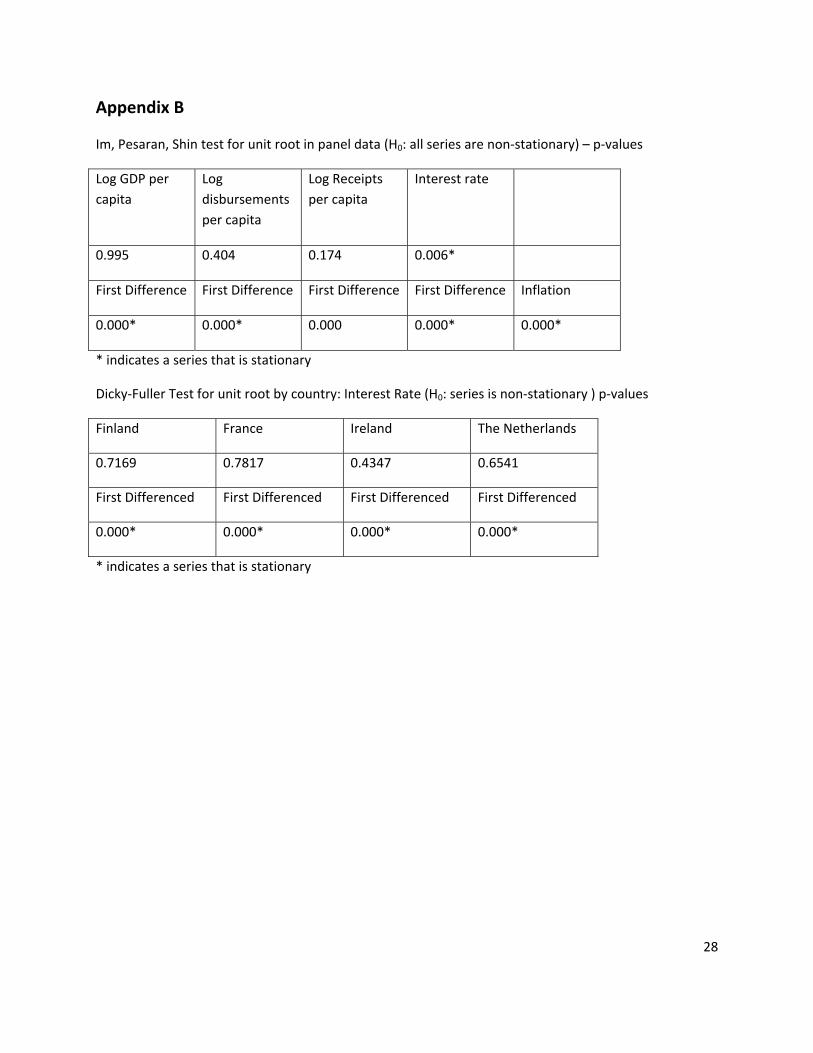
It is important that each series used in the VAR be stationary to obtain consistent estimates of

the parameters and impulse response functions. Each of the panel series were tested for stationarity

with Im, Pesaran, Shin (2003) tests for unit roots in a panel series (results posted in Appendix B). The

test rejects the null hypothesis of non‐stationarity for the inflation and short term interest rate series.

The test indicates that in the case of logged GDP, spending, and revenue per capita we must fail to reject

the null hypothesis. As a result the first difference of the logged GDP, disbursement, and receipt per

capita are used in the VAR (all of which are stable according to the Im, Pesara, and Shin test). Close

inspection of the interest rate series for each of these countries does show a pronounced downward

trend. This is a product of the time period over which the sample covers. Oil shocks in the 1970s caused

high inflation to which monetary authorities across Europe responded with tight monetary policy. Since

that time rates have steadily fallen as inflation was brought under control, allowing for looser monetary

policy. In addition, the Maastricht treaty required convergence to a lower interest rate in preparation

for joining the union. Dicky‐Fuller stationarity tests of the interest rate series for each country in this

sample indicate that the series is not stationary. Therefore the interest rate series is also first

17

differenced for use in the VAR7. A lag length of two is used in the VAR.

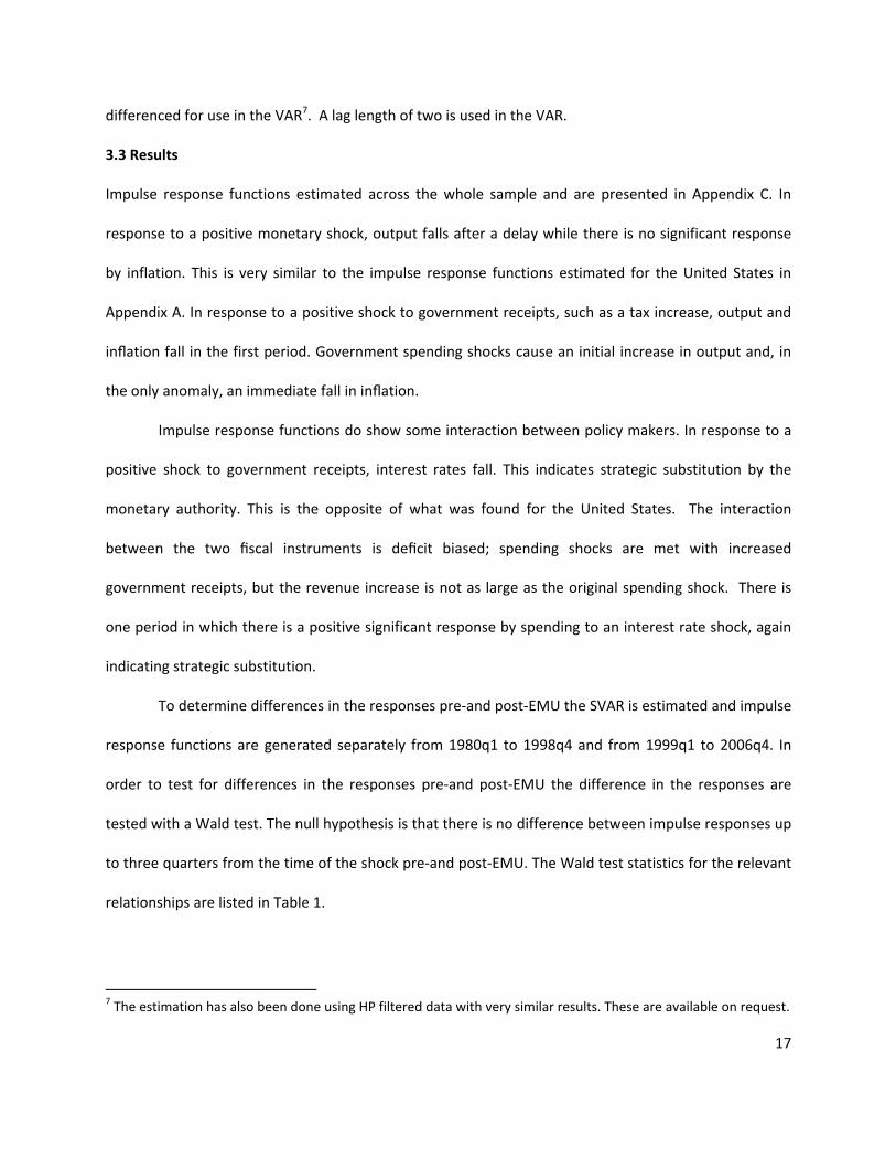
3.3 Results

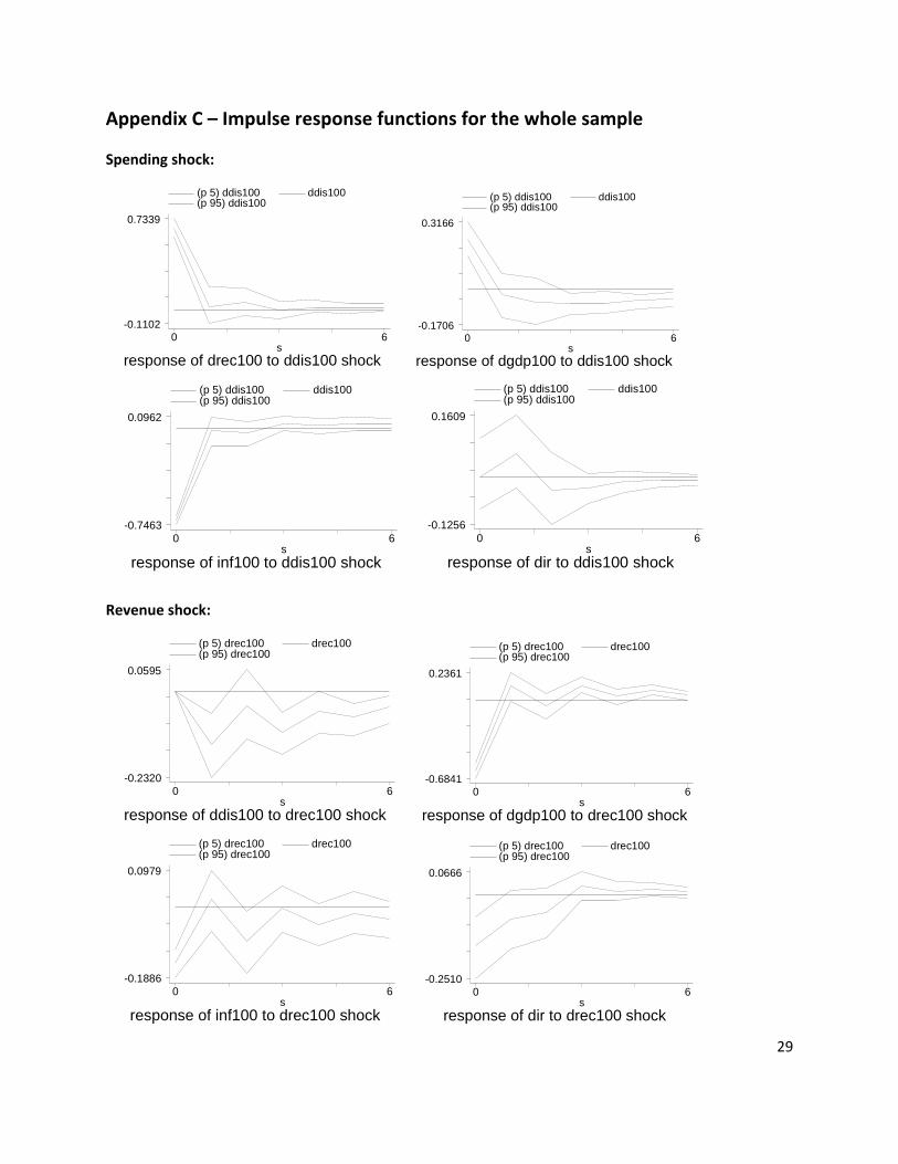
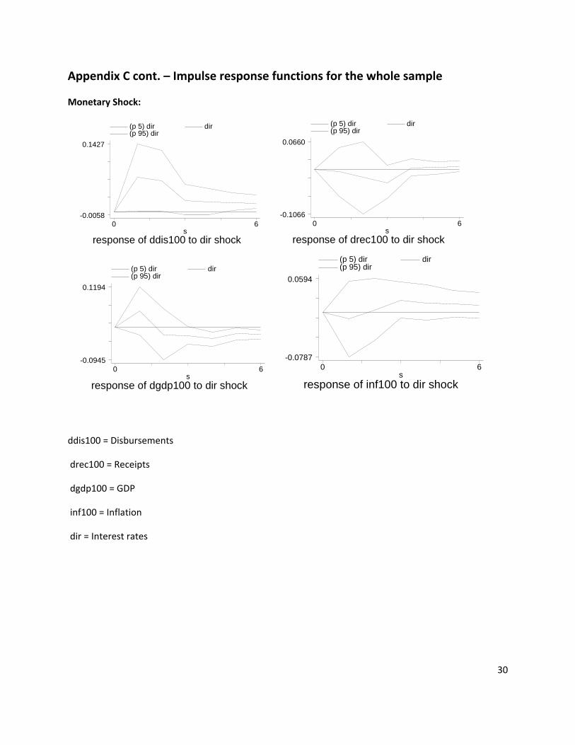
Impulse response functions estimated across the whole sample and are presented in Appendix C. In

response to a positive monetary shock, output falls after a delay while there is no significant response

by inflation. This is very similar to the impulse response functions estimated for the United States in

Appendix A. In response to a positive shock to government receipts, such as a tax increase, output and

inflation fall in the first period. Government spending shocks cause an initial increase in output and, in

the only anomaly, an immediate fall in inflation.

Impulse response functions do show some interaction between policy makers. In response to a

positive shock to government receipts, interest rates fall. This indicates strategic substitution by the

monetary authority. This is the opposite of what was found for the United States. The interaction

between the two fiscal instruments is deficit biased; spending shocks are met with increased

government receipts, but the revenue increase is not as large as the original spending shock. There is

one period in which there is a positive significant response by spending to an interest rate shock, again

indicating strategic substitution.

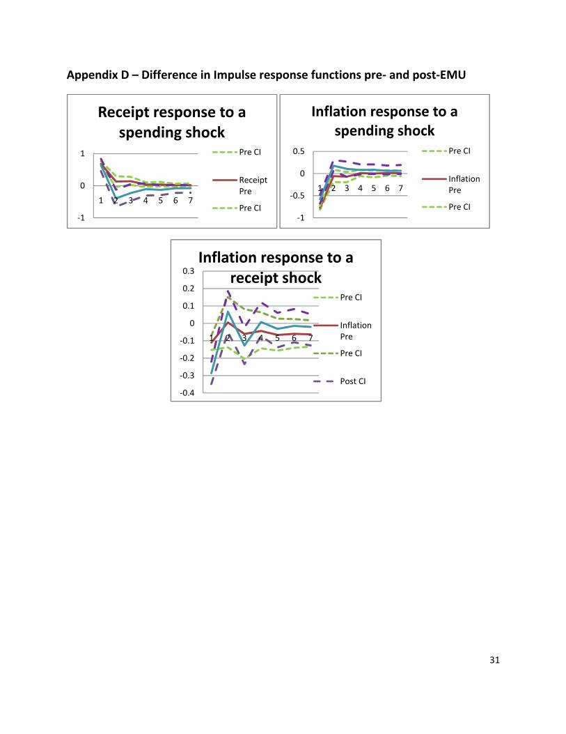
To determine differences in the responses pre‐and post‐EMU the SVAR is estimated and impulse

response functions are generated separately from 1980q1 to 1998q4 and from 1999q1 to 2006q4. In

order to test for differences in the responses pre‐and post‐EMU the difference in the responses are

tested with a Wald test. The null hypothesis is that there is no difference between impulse responses up

to three quarters from the time of the shock pre‐and post‐EMU. The Wald test statistics for the relevant

relationships are listed in Table 1.

7 The estimation has also been done using HP filtered data with very similar results. These are available on request.

18

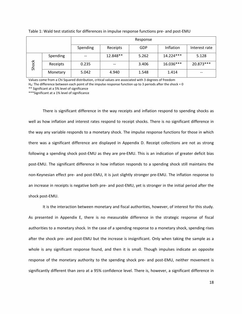
Table 1: Wald test statistic for differences in impulse response functions pre‐ and post‐EMU

Response

Spending Receipts GDP Inflation Interest rate

Shock

Spending ‐‐ 12.848** 5.262 14.224*** 5.128

Receipts 0.235 ‐‐ 3.406 16.036*** 20.873***

Monetary 5.042 4.940 1.548 1.414 ‐‐

Values come from a Chi Squared distribution, critical values are associated with 3 degrees of freedom H0: The difference between each point of the impulse response function up to 3 periods after the shock = 0 ** Significant at a 5% level of significance ***Significant at a 1% level of significance

There is significant difference in the way receipts and inflation respond to spending shocks as

well as how inflation and interest rates respond to receipt shocks. There is no significant difference in

the way any variable responds to a monetary shock. The impulse response functions for those in which

there was a significant difference are displayed in Appendix D. Receipt collections are not as strong

following a spending shock post‐EMU as they are pre‐EMU. This is an indication of greater deficit bias

post‐EMU. The significant difference in how inflation responds to a spending shock still maintains the

non‐Keynesian effect pre‐ and post‐EMU, it is just slightly stronger pre‐EMU. The inflation response to

an increase in receipts is negative both pre‐ and post‐EMU, yet is stronger in the initial period after the

shock post‐EMU.

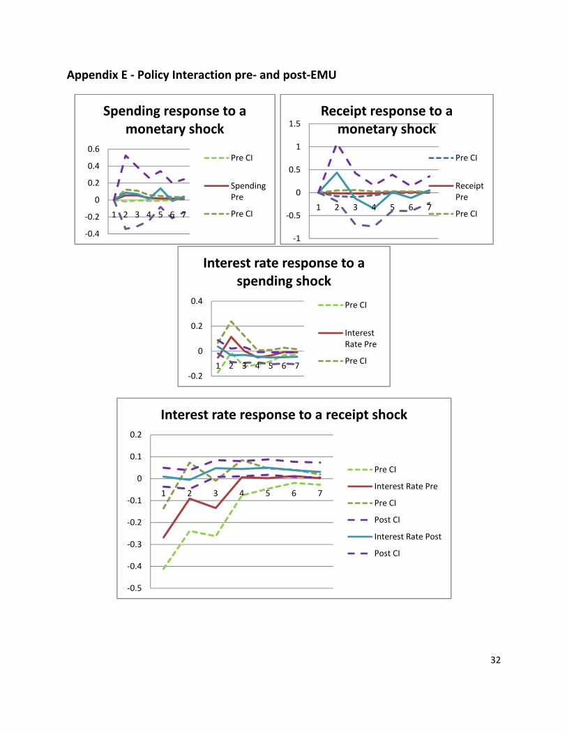
It is the interaction between monetary and fiscal authorities, however, of interest for this study.

As presented in Appendix E, there is no measurable difference in the strategic response of fiscal

authorities to a monetary shock. In the case of a spending response to a monetary shock, spending rises

after the shock pre‐ and post‐EMU but the increase is insignificant. Only when taking the sample as a

whole is any significant response found, and then it is small. Though impulses indicate an opposite

response of the monetary authority to the spending shock pre‐ and post‐EMU, neither movement is

significantly different than zero at a 95% confidence level. There is, however, a significant difference in

19

how the monetary authority responds to a receipt shock. Pre‐EMU there is statistically significant

strategic substitution. As receipts rise through a discretionary increase in taxes or some other revenue

source designed to dampen economic activity, interest rates fall and in order to stimulate economic

activity. Post‐EMU there is no such interplay, the ECB does not respond strategically to tax changes.

This outcome could signify that as a result of joining a union any strategic interplay is lost.

Before the monetary union monetary and fiscal authorities, though independent of each other, where

working towards accomplishing national goals and were indirectly or directly in contact and

communication with each other. After the union, however, the European Central Bank is much further

removed from the fiscal authority and the individual countries needs. They respond to aggregate levels

of data. Just as the ECB is unable to respond to individual member’s asymmetric fluctuations, which are

lost in the union aggregate, so too is the ECB unable to respond to individual fiscal movements. This

greater “distance” as a result of joining the union could have caused the change in strategic interaction.

This finding could also be due to differences in the types of shocks hitting the economy pre‐ and

post‐EMU. Buti et al (2007) and Van Aarle et al (2004) find that the interaction between monetary and

fiscal policies are shock dependent. Their models indicate that the gains to policy coordination in the

presence of demand shocks are low, whereas supply shocks lead to greater coordination. The loss of

strategic interaction detected in the data could therefore be a manifestation of fewer supply shocks or

more demand shocks hitting the economy post‐EMU. Though there is no structural reason that a

monetary union would cause such a shift in the shock structure of the European economy, these

estimation techniques cannot dismiss this as a possibility.

Yet another explanation of the change in the interaction between policy makers lies in the

specific convergence criteria put in place in the run up to joining the monetary union. The Maastricht

Treaty required not only stable exchange rates, but similarity in inflation and interest rates across

potential members. In the case of many potential members this required a significant reduction in

20

inflation. In addition budget deficits were restricted, which by the time the country joined the EMU had

to be within 3 percent of GDP. This particular restriction required significant deficit reductions for many

of the potential members. The strategic substitution evident pre‐EMU could be an indication of one

authority softening the blow (in terms of output) of the others policy used to meet the Maastricht

criteria. For example a large increase in interest rates to bring down inflation would be met with a

reduction in taxes to mitigate the future output effects of the monetary retraction. On the other hand,

an increase in taxes in order to reduce deficit levels could be met with a loosening of monetary policy in

order to mitigate the output effects of increased taxes.

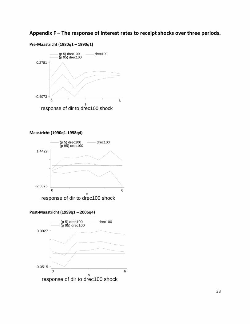
Though data is limited, the sample is split up into three periods: the pre Maastricht period

(1980q1 – 1991q1), the Maastricht period (1990q1 ‐ 1998q4), and the post Maastricht period (1999q1 ‐

2006q4).8 The response of interest rates to revenue shocks are presented in Appendix F. Only during the

Maastricht period is there significant strategic interaction. In contrast to von Hagen et al (2000),

interaction is greater during the Maastricht period. Their study however did not measure monetary

reactions to fiscal policy, which is where interaction is detected in this study. Direct causation is not

rigorously explored in this particular study, but the findings do indicate that the convergence criteria did

play an important role in strategic monetary and fiscal interaction among European countries.

4. Conclusions and extensions

Entering a monetary union potentially changes the structure and relationship among and within

members of the union. The act of giving up a national currency, and the inherent control and

8 The Maastricht treaty was signed in 1992, but the first stage of the Delors recommendations were put in place in

1990. Thus 1990 signified the application of the Delors report which would inevitably lead to a monetary union.

This is the period chosen to represent the start of the Maastricht period as it signifies the beginning of the

unification in earnest and provides a maximum number of observations for the VAR.

21

individuality of that currency, in order to gain the supposed economic advantages of a common currency

requires tremendous political will and the surrender of some economic independence. The effects of the

great European monetary experiment are just beginning to be studied as data become available. This

paper addresses one possible cost/benefit from joining a monetary union, the change in the relationship

and strategic interaction of the monetary and fiscal authority.

This paper finds that in one particular case, the response of the monetary authority to a fiscal

receipts shock, the formation of the EMU did lead to a different strategic reaction. Pre‐EMU the

monetary and fiscal authority in this particular combination acted as strategic substitutes; if taxes or

other revenue sources were raised the local monetary authority would lower the interest rate. After the

formation of the union this relationship disappears and there is no strategic interaction. The cause of

this change is not addressed directly from this study, but one possible explanation is the “distance” a

monetary union places between the new union‐wide monetary authority and the individual member

fiscal authority. The observation that the substitutability only occurs during the Maastricht period,

however, suggests that this result is more a feature of the convergence criteria put in place in the run up

to joining the EMU coupled with a weak SGP. In many cases significant inflation and/or deficit reduction

measure were undertake in order to qualify, according to the Maastricht treaty, for membership in

monetary union. Only during the Maastricht period is this strategic interaction detected. The strategic

substitution indicates that monetary and fiscal authorities (through government receipts) worked

together soften the blow if each other’s actions in order to join the union.

One remaining explanation comes from the nature of shocks that hit the economy. Theoretical

models indicate that policy interaction is more prevalent in the case of supply shocks, while the gains to

coordination are diminished in the face of demand shocks. If the nature of the shocks hitting the

European economies changed over this period of time the interaction might of as well. If this were the

cause of the change in policy interaction, one would expect less supply shocks or a greater prevalence of

22

demand shocks post‐EMU. The techniques used in this study, however, do not allow for a measure of

supply and demand shocks. Van Aarle, Garretsen, and Gobbin (2003) use long‐run restrictions to identify

both monetary and fiscal shocks as well as supply and demand shocks. Possible extensions using similar

restrictions could help answer this question.

Because the Maastricht period, with is strict convergence criteria, was so successful in reducing

deficits and inflation across the European nations it would seem that the strategic substitution would be

helpful in such extreme times. Would EMU members profit from continued strategic interaction

between policy makers once in the monetary union? This is also a question yet to be answered in the

literature in general. Further work should include some way of measuring the costs and benefits of such

strategic interaction.

23

References:

Van Aarle, B., H. Garretsen, & F. Huart (2004) Monetary and fiscal policy rules in the EMU. German

Economic Review 5, 407-434.

Van Aarle, B., H. Garretsen, & N. Gobbin (2003) Monetary and fiscal policy transmission in the Euro-area:

Evidence from a structural VAR analysis. Journal of Economics and Business 55, 609-638.

Afxentiou, P. (2000) Convergence, Maastricht criteria, and their benefits. The Brown Journal of World Affairs

7, 245-254.

Arellano, M. & O. Bover (1995) Another look at the instrumental variable estimation of error-components

models. Journal of Econometrics 68, 29–51.

Pierpaolo B. & M. Woodford (2003) Optimal monetary and fiscal policy: A linear quadratic approach," NBER

Working Papers 9905, National Bureau of Economic Research, Inc.

Blachard , O. & R. Perotti (2002) An empirical characterization of the dynamic effects of changes in

government spending and taxes on output. Quarterly Journal of Economics 117, 1329-1368.

Buti, M., W. Roeger, & J. In’t Veld (2001) Stabilizing output and inflation: Policy conflicts and co-operation

under a stability pact. Journal of Common Market Studies 39, 801-28.

Caldara, D. & C. Kamps (2008) What are the effects of fiscal policy shocks? A VAR –based comparative

analysis. European Central Bank Working Papers Series No. 877.

Canzoneri, M., R. Cumby, & B. Diba (2002) Should the European Central Bank and the Federal Reserve be

concerned about fiscal policy. Presented at the Federal Reserve Bank of Kansas City’s Symposium on

Rethinking Stabilization Policy.

Christiano, L., M. Eichenbaum, & C. Evans (1999) Monetary policy shocks: What have we learned and to

what end. Working Paper.

Claey, P. (2006) Policy mix and debt sustainability: evidence from fiscal policy rules. Empirica 33, 89-112.

Fatas, A. & I. Mihov (2001) The effects of fiscal policy on consumption and employment: Theory and

evidence. CEPR Discussion Paper No. 2760.

24

Favero, C. (2002) “How do European monetary and fiscal authorities behave?” IGIER Working Paper No.

214.

Governatori, M. & S. Eijffinger (2004) Fiscal and monetary interaction: The role of asymmetries of the

Stability and Growth Pact in EMU. CESifo Working Paper No. 1354.

Giorono, C., P. Richardson, D. Roseveare, & P. van der Noord (1995) Potential output, output gaps , and

structural budget balances. OECD Economic Studies No. 24.

von Hagen, J., Hallett, A.H., & Strauch, R. (2001) Budgetary Consolidation in EMU. European Economy -

Economic Papers 148, Commission of the EC, Directorate-General for Economic and Financial Affairs

(DG ECFIN).

Jordi G. & T. Monacelli (2005) Optimal monetary and fiscal policy in a currency union. Economics Working

Papers 909, Department of Economics and Business, Universitat Pompeu Fabra, revised Feb 2008

Gali, J. & R. Perrotti (2003) Fiscal policy and monetary integration in Europe. Economic Policy 18.

IMF staff (2004) Has fiscal behavior changed under the European economic and monetary Union? In World

Economic Outlook, 103-136.

Leith, C. & S. Wren-Lewis (2000) Interaction between monetary and fiscal policy rules. The Economic

Journal 110, C93-C108.

Love, I. (2001) Estimating panel-data autoregressions. Package of Programs for STATA, Columbia

University, Mimeo.

Love, I. (2006) Financial development and dynamic investment behaviour: Evidence for panel VAR. The

Quarterly Review of Economic and Finance 46, 190–210.

Mélitz, J (1997) Some cross-country evidence about debt, deficits and the behaviour of monetary and fiscal

authorities," CEPR Discussion Papers 1653, C.E.P.R. Discussion Papers.

Mountford, A. & H. Uhlig (2005) What are the effects of fiscal policy shocks? SFB 649 Discussion Paper no.

39. Humbolt University, Berlin.

Mundell, R. (1961) A theory of optimal currency area. American Economic Review 51.

25

Muscatelli, A., P. Tirelli, & C. Trecroci (2004) Monetary and fiscal policy interaction over the cycle: Some

empirical evidence. In Beetsma, R., C. Favero, A. Missala, A. Muscatelli, P. Natale, and P. Tirelli (Eds.),

Fiscal Policies, Monetary Policies and Labour markets, Key Aspects of European Macroeconomic

Policies After Monetary Unification. Cambridge University Press, Cambridge UK.

Perotti, R. (2004) Estimating the effects of fiscal policy on OECD countries. IGIER Working Paper No. 276.

Ramey, V. & M. Shapiro (1998) Costly capital reallocation and the effects of government spending. Carnegie-

Rochester Conferince Series on Public Policy 48 (June): 145-194.

Wickens, T. (2002). Government Finance Statistical Manual 2001 Companion Material: Classifications of

GFSM 1986 data to the GFSM 2001 framework. IMF.

26

Appendix A

Blanchard and Perroti Restrictions (BPR) – US data

Shock 1 = Government spending shock Shock 4 = Government receipts shock Shock 5 = Monetary shock Lrdis1000cap = Spending reaction Lrrec1000cap = Receipts reaction Lrgdp1000cap = Output reaction Inf_log = Inflation reaction Ir = Interest rate reaction

-1.0

-0.5

0.0

0.5

1.0

1.5

1 2 3 4 5 6 7 8 9 10

Response of LRDIS1000CAP to Shock1

-1.0

-0.5

0.0

0.5

1.0

1.5

1 2 3 4 5 6 7 8 9 10


-1.0

-0.5

0.0

0.5

1.0

1.5

1 2 3 4 5 6 7 8 9 10


-4

-2

0

2

4

1 2 3 4 5 6 7 8 9 10

Response of LRREC1000CAP to Shock1

-4

-2

0

2

4

1 2 3 4 5 6 7 8 9 10


-4

-2

0

2

4

1 2 3 4 5 6 7 8 9 10


-2.0

-1.5

-1.0

-0.5

0.0

0.5

1.0

1 2 3 4 5 6 7 8 9 10

Response of LRGDP1000CAP to Shock1

-2.0

-1.5

-1.0

-0.5

0.0

0.5

1.0

1 2 3 4 5 6 7 8 9 10


-2.0

-1.5

-1.0

-0.5

0.0

0.5

1.0

1 2 3 4 5 6 7 8 9 10


-.4

-.2

.0

.2

.4

.6

1 2 3 4 5 6 7 8 9 10

Response of INF_LOG to Shock1

-.4

-.2

.0

.2

.4

.6

1 2 3 4 5 6 7 8 9 10


-.4

-.2

.0

.2

.4

.6

1 2 3 4 5 6 7 8 9 10


-2

-1

0

1

2

3

1 2 3 4 5 6 7 8 9 10

Response of IR to Shock1

-2

-1

0

1

2

3

1 2 3 4 5 6 7 8 9 10


-2

-1

0

1

2

3

1 2 3 4 5 6 7 8 9 10


Response to Structural One S.D. Innovations ± 2 S.E.

27

Appendix A continued

My Restrictions (MR) ‐ US data

Shock 1 = Government spending shock Shock 2 = Government receipts shock Shock 5 = Monetary shock Lrdis1000capca = Spending reaction Lrrec1000capca = Receipts reaction Lrgdp1000cap = Output reaction Inf_log = Inflation reaction Ir = Interest rate reaction

-1.0

-0.5

0.0

0.5

1.0

1.5

1 2 3 4 5 6 7 8 9 10

Response of LRDIS1000CAPCA to Shock1

-1.0

-0.5

0.0

0.5

1.0

1.5

1 2 3 4 5 6 7 8 9 10


-1.0

-0.5

0.0

0.5

1.0

1.5

1 2 3 4 5 6 7 8 9 10


-1.0

-0.5

0.0

0.5

1.0

1.5

2.0

1 2 3 4 5 6 7 8 9 10

Response of LRREC1000CAPCA to Shock1

-1.0

-0.5

0.0

0.5

1.0

1.5

2.0

1 2 3 4 5 6 7 8 9 10


-1.0

-0.5

0.0

0.5

1.0

1.5

2.0

1 2 3 4 5 6 7 8 9 10


-0.5

0.0

0.5

1.0

1 2 3 4 5 6 7 8 9 10


-0.5

0.0

0.5

1.0

1 2 3 4 5 6 7 8 9 10


-0.5

0.0

0.5

1.0

1 2 3 4 5 6 7 8 9 10


-.3

-.2

-.1

.0

.1

.2

.3

1 2 3 4 5 6 7 8 9 10


-.3

-.2

-.1

.0

.1

.2

.3

1 2 3 4 5 6 7 8 9 10


-.3

-.2

-.1

.0

.1

.2

.3

1 2 3 4 5 6 7 8 9 10


-1.5

-1.0

-0.5

0.0

0.5

1.0

1.5

1 2 3 4 5 6 7 8 9 10


-1.5

-1.0

-0.5

0.0

0.5

1.0

1.5

1 2 3 4 5 6 7 8 9 10


-1.5

-1.0

-0.5

0.0

0.5

1.0

1.5

1 2 3 4 5 6 7 8 9 10


Response to Structural One S.D. Innovations ± 2 S.E.

28

Appendix B

Im, Pesaran, Shin test for unit root in panel data (H0: all series are non‐stationary) – p‐values

Log GDP per

capita

Log

disbursements

per capita

Log Receipts

per capita

Interest rate

0.995 0.404 0.174 0.006*

First Difference First Difference First Difference First Difference Inflation

0.000* 0.000* 0.000 0.000* 0.000*

* indicates a series that is stationary

Dicky‐Fuller Test for unit root by country: Interest Rate (H0: series is non‐stationary ) p‐values

Finland France Ireland The Netherlands

0.7169 0.7817 0.4347 0.6541

First Differenced First Differenced First Differenced First Differenced

0.000* 0.000* 0.000* 0.000*

* indicates a series that is stationary

29

Appendix C – Impulse response functions for the whole sample

Spending shock:

Revenue shock:

response of drec100 to ddis100 shocks

(p 5) ddis100 ddis100 (p 95) ddis100

0 6-0.1102

0.7339

response of dgdp100 to ddis100 shocks

(p 5) ddis100 ddis100 (p 95) ddis100

0 6-0.1706

0.3166

response of inf100 to ddis100 shocks

(p 5) ddis100 ddis100 (p 95) ddis100

0 6-0.7463

0.0962

response of dir to ddis100 shocks

(p 5) ddis100 ddis100 (p 95) ddis100

0 6-0.1256

0.1609

response of ddis100 to drec100 shocks

(p 5) drec100 drec100 (p 95) drec100

0 6-0.2320

0.0595

response of dgdp100 to drec100 shocks

(p 5) drec100 drec100 (p 95) drec100

0 6-0.6841

0.2361

response of inf100 to drec100 shocks

(p 5) drec100 drec100 (p 95) drec100

0 6-0.1886

0.0979

response of dir to drec100 shocks

(p 5) drec100 drec100 (p 95) drec100

0 6-0.2510

0.0666

30

Appendix C cont. – Impulse response functions for the whole sample

Monetary Shock:

ddis100 = Disbursements

drec100 = Receipts

dgdp100 = GDP

inf100 = Inflation

dir = Interest rates

response of ddis100 to dir shocks

(p 5) dir dir (p 95) dir

0 6-0.0058

0.1427

response of drec100 to dir shocks


0 6-0.1066

0.0660

response of dgdp100 to dir shocks


0 6-0.0945

0.1194

response of inf100 to dir shocks


0 6-0.0787

0.0594

31

Appendix D – Difference in Impulse response functions pre‐ and post‐EMU

‐1

0

1

1 2 3 4 5 6 7

Receipt response to a spending shock

Pre CI

Receipt Pre

Pre CI‐1

‐0.5

0

0.5

1 2 3 4 5 6 7

Inflation response to a spending shock

Pre CI

Inflation Pre

Pre CI

‐0.4

‐0.3

‐0.2

‐0.1

0

0.1

0.2

0.3

1 2 3 4 5 6 7

Inflation response to a receipt shock

Pre CI

Inflation Pre

Pre CI

Post CI

32

Appendix E ‐ Policy Interaction pre‐ and post‐EMU

‐0.4

‐0.2

0

0.2

0.4

0.6

1 2 3 4 5 6 7

Spending response to a monetary shock

Pre CI

Spending Pre

Pre CI

‐1

‐0.5

0

0.5

1

1.5

1 2 3 4 5 6 7

Receipt response to a monetary shock

Pre CI

Receipt Pre

Pre CI

‐0.2

0

0.2

0.4

1 2 3 4 5 6 7

Interest rate response to a spending shock

Pre CI

Interest Rate Pre

Pre CI

‐0.5

‐0.4

‐0.3

‐0.2

‐0.1

0

0.1

0.2

1 2 3 4 5 6 7

Interest rate response to a receipt shock

Pre CI

Interest Rate Pre

Pre CI

Post CI

Interest Rate Post

Post CI

33

Appendix F – The response of interest rates to receipt shocks over three periods.

Pre‐Maastricht (1980q1 – 1990q1)

Maastricht (1990q1‐1998q4)

Post‐Maastricht (1999q1 – 2006q4)


(p 5) drec100 drec100 (p 95) drec100

0 6-0.4073

0.2781


(p 5) drec100 drec100 (p 95) drec100

0 6-2.0375

1.4422


(p 5) drec100 drec100 (p 95) drec100

0 6-0.0515

0.0927

Documents

Monetary and Fiscal Policy Interaction: The Consequences ...aei.pitt.edu/33072/1/jones._jason_cannon.pdf · Monetary and Fiscal Policy Interaction: ... Monetary and Fiscal Policy