1

Chapter 7 Modal Testing

The use of our analytical methods to date to interpret vibration

measurementsA standard skill used in industry

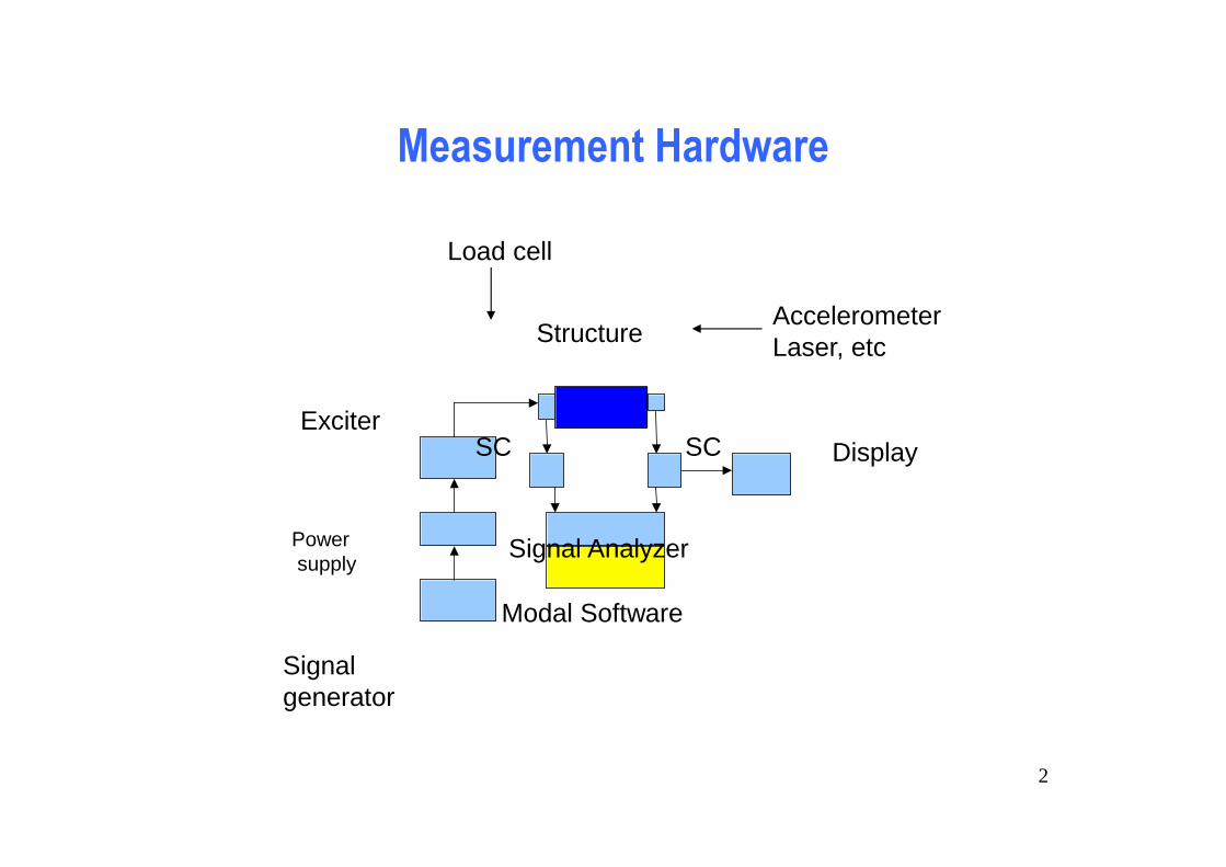
Measurement Hardware

Structure

Exciter

Powersupply

Signal generator

SC SC

Signal Analyzer

Modal Software

Display

AccelerometerLaser, etc

Load cell

2

Transducer

• Load cell: a piezoceramic device configured to produce a voltage proportional to force

• Accelerometer (also based on piezoceramic) produce a signal proportional to acceleration at the point of attachment

3

• Proximity probes, usually magnetic and give a signal proportional to local displacement

• Laser vibrometers give a signal proportional to local velocity (or scanned to give velocity

• field) or displacement

• Strain gauges (local strain or strain rate)

• Others

4

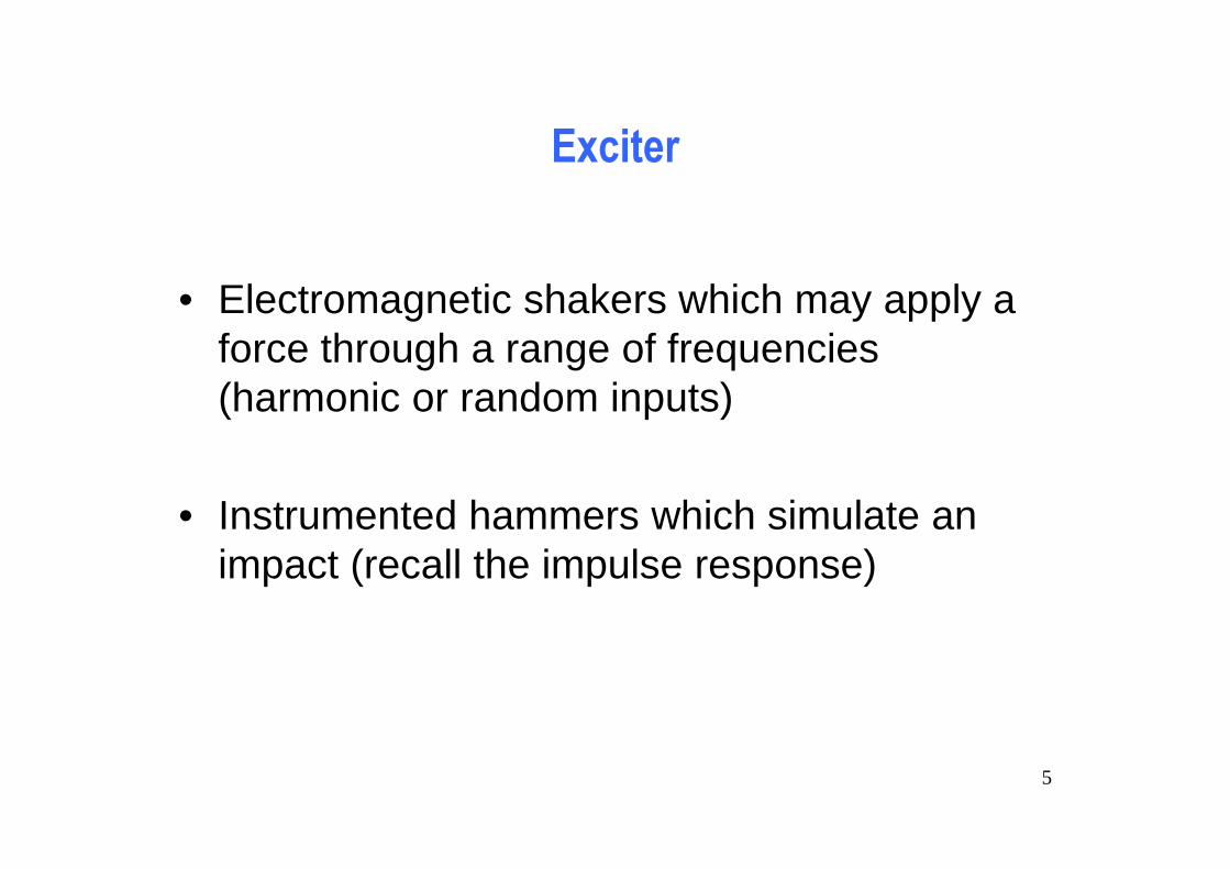
Exciter

• Electromagnetic shakers which may apply a force through a range of frequencies (harmonic or random inputs)

• Instrumented hammers which simulate an impact (recall the impulse response)

5

Signal Conditioning

• The direct out put of a transducer not usually well suited for input into an analyzer

• Impedance miss matched, voltage or current levels too low

• SC is a charge or voltage amp designed to take an accelerometer signal and match it to the input requirements of the analyzer

6

Analyzer

• Electronic boxes (really dedicated computers) which gather signals and manipulate them mathematically

• Like all other computer based technologies the analyzer “boxes” have evolved almost in to chip sized devices

• Essentially their main source of manipulation is digital Fourier Transforms for manipulating the vibration data in the frequency domain

7

Frequency Spectrum of a typical Hammer Hit

Cut off frequency8

Fourier Series

x(t) =a

0

2+ (a

ncos nω

Tt +

n=1

∞

∑ bnsin nω

Tt) (8.1)

where ωT

=2πT

a0

=2

Tx(t)dt

0

T

∫

an

=2

Tx(t)cos nω

Ttdt

0

T

∫ n = 1,2,3....

bn

=2

Tx(t)sin nω

Ttdt

0

T

∫ n = 1,2,3.... (8.2)

9

Signal and Fourier spectrum

10

Spectrum Analyzer

• Analog voltage in from force f(t) and one of x(t), v(t) or a(t) transducers

• Signals are filtered, “digitized” and transformed to the frequency domain

• Manipulated to produce digital frequency response functions from which vibration data is extracted

11

Digital Signal Processing(DSP)

• The analyzer takes signals form the transducer and puts the signal into a form that can be mathematically manipulated

• This of course is best performed with digital computers, hence we rely on some basic principles of dps

12

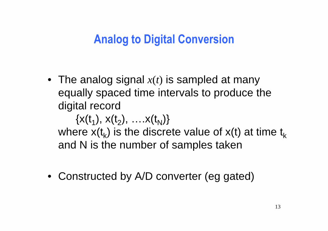
Analog to Digital Conversion

• The analog signal x(t) is sampled at many equally spaced time intervals to produce the digital record

{x(t1), x(t2), ….x(tN)}where x(tk) is the discrete value of x(t) at time tkand N is the number of samples taken

• Constructed by A/D converter (eg gated)

13

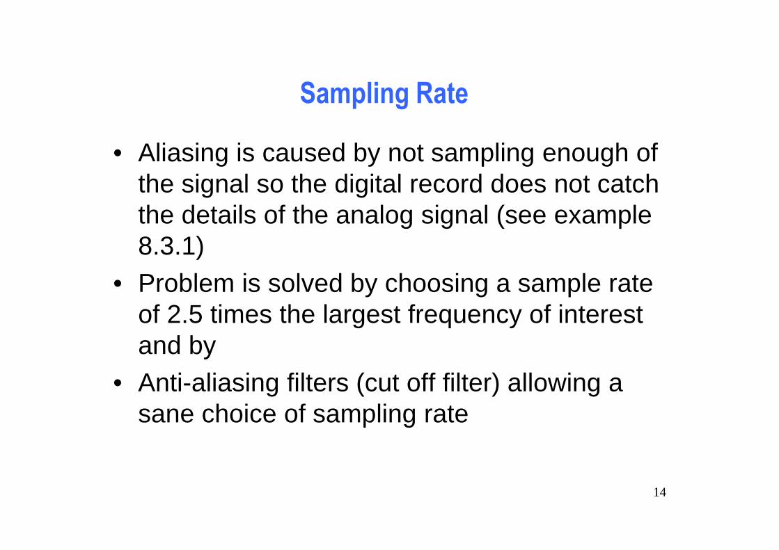
Sampling Rate

• Aliasing is caused by not sampling enough of the signal so the digital record does not catch the details of the analog signal (see example 8.3.1)

• Problem is solved by choosing a sample rate of 2.5 times the largest frequency of interest and by

• Anti-aliasing filters (cut off filter) allowing a sane choice of sampling rate

14

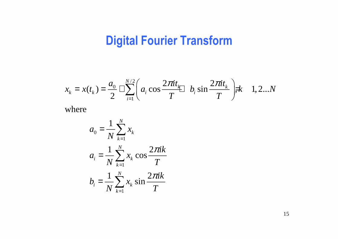
Digital Fourier Transform

/ 20

1

01

1

1

2 2( ) cos sin , 1,2...

2

where

1

1 2 cos

1 2 sin

Nk k

k k i ii

N

kk

N

i kk

N

i kk

a it itx x t a b k N

T T

a xN

ika x

N T

b xN

π π

π

=

=

=

=

= = + + =

=

=

=

∑

∑

∑

∑ik

T

π

15

FFT/DFT Analyzer

• Above becomes the matrix equation x=Ca where C contains the sin and cos termsx is the vector of samples anda is the vector of Fourier Coefficients

• The analyzer computes the coefficients in the DFT formula by a=C-1x

• N is fixed by hardware (a power of 2)

16

Leakage and Windowing

Leakage Hanning window

17

Random Signal Analysis

0

0

1Autocorrelation: ( ) lim ( ) ( )

1Power Spectral Density (PSD): ( ) ( )

2

1Crosscorrelation: ( ) lim ( ) ( )

1Cross Spectral Density: ( ) ( )

2

T

xxT

jxx xx

T

xfT

jxf xf

R x t x t dT

S R e d

R x t f t dT

S R e d

ωτ

ωτ

τ τ τ

ω τ τπ

τ τ τ

ω τ τπ

→∞

∞−

−∞

→∞

−

−

= +

=

= +

=

∫

∫

∫∞

∞∫

Tells how fast x(t) is changing

Fourier transform of R

Tells how fast one signal changesrelative to another

18

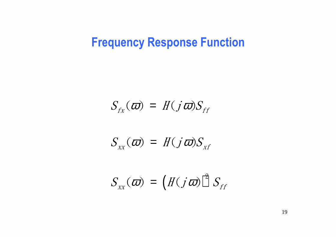
Frequency Response Function

( )

ω ω

ω ω

ω ω

=

=

= 2

( ) ( )

( ) ( )

( ) ( )

fx ff

xx xf

xx ff

S H j S

S H j S

S H j S

19

( (

( (

2

2

2

2

22

0

1( )

1( ) ( )

1( ) sin

1 [ ( )] ( )

( ) deterministic ( ) random

( ) ( ) ( ) ( ) ( ) ( )

( ) ( ) ( ) [ ] ( ) ( )

td

d

xx ff

t

ff

G sms cs k

G j Hk m cj

h t e tm

LT h t G sms cs k

f t f t

X s G s F s S H S

x t h t f d E x H S d

ζω

ω ωω ω

ωω

ω ω ω

τ τ τ ω ω ω

−

∞

−∞

=+ +

= =− +

=

= =+ +

= =

= − =∫ ∫

Transfer function

Frequency response function

Impulse response function

20

• PSD’s calculated in analyzer

• Used to form H(ω) for force in, response out (velocity, position or acceleration)

• H(ω) used to extract modal data of structure in a number of different ways, forming the topic of Modal Testing

21

Coherence

γ 2 =Sxf (ω)

2

Sxx (ω)S ff (ω)

0 ≤ γ 2 ≤1

should be 1, especially

near resonance

• Compute H(ω) a number of different ways

• Compare the various measured values of H(ω)

• Indicates how good the measurement is

22

Transfer function nomenclature

2( ) ( ) ( )( ) ( ) ( )

( ) ( ) ( )

standard

Displacement compliance dynamic stiffness

Velocity mobility impedance

Acceleration inertance apparent mass

X s sX s s X sG s G s G s

F s F s F s

response reciprical

= = =

23

Measured Compliance FRF

Illustrates peak picking methodof determining modal parameters

Natural frequency taken as peak value

24

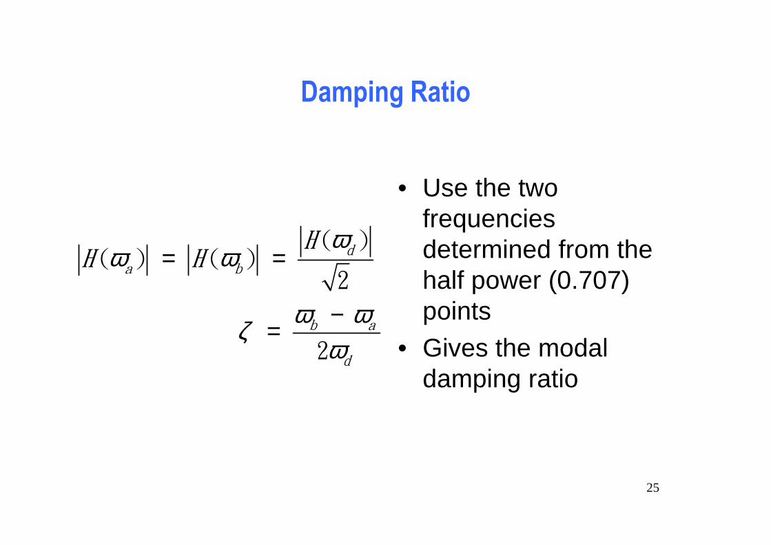
Damping Ratio

( )( ) ( )

2

2

da b

b a

d

HH H

ωω ω

ω ωζω

= =

−=

• Use the two frequencies determined from the half power (0.707) points

• Gives the modal damping ratio

25

Example Response with two modes:

First modesecond mode

1

12

10.16 9.750.02

20

b aω ωζω−

=

−= =

2

22

21.67 17.10

40

0.11

b aω ωζω−

=

−=

=

26

Mode shape measurement

2

2 1

2 1

2 2 1

,

( )

( )

( ) ( )

[ diag( 2 ) ]

j t j t

i i i

x e e

j

j

j

j

ω ω

ω ωω ω

α ω ω ωω ω ζ ω

−

−

−

+ + = =− + =

= − += − += − +

M x Kx f x u

K M u f

u K M f

K M

ɺɺ ɺ

T

D

D

D

D

V V

27

Need only one column to get mode shape

Suppose ui = [a1 a2 a3]T

uiuiT =

a12 a1a2 a1a3

a2a1 a22 a2a3

a3a1 a3a2 a32

really only 3 unkowns a1, a2 and a3 . So just three

elements of α(ω) need be measured per mode to get

the mode shape

28

29

Model Updating

• All analytical models must be verified by experiments

• Often the experimental data will disagree slightly with the analytical model

• If this is the case, the analytical model is often adjusted (hopefully slightly) so that the adjusted, or updated, model agrees with experimentally measured data

• Many papers and one book have been written on this topic and it is still one of active research

30