NASA Contractor Report 3429

Analytical Testing

W. G. Flannelly, J. A. Fabunmi, and E. J. Nagy

CONTRACT NASl-15414 MAY 1981

https://ntrs.nasa.gov/search.jsp?R=19810014954 2018-07-17T01:10:20+00:00Z

NASA Contractor Report 3429

Analytical Testing

W. G. Flannelly, J. A. Fabunmi, and E. J. Nagy Kaman Aerospace Corporation Bloomfield, Cotlnecticut

Prepared for Langley Research Center under Contract’ NASl-15414

National Aeronautics and Space Administration

Scientific and Technical Information Branch

TECH LIBRARY KAFB, NM

ll~llllRllll~llmallRlli OObL979

1981

TABLE OF CONTENTS

PAGE NO.

SUMMARY ..............................

INTRODUCTION. ...........................

LIST OF SYMBOLS ..........................

THE PRACTICAL ASPECTS OF ANALYTICAL TESTING ............

ANALYTICAL TESTING THEORY .....................

Types of Mobilities. .....................

Analytical Testing Equations .................

Limitations of the Method. ..................

APPLICATIONS OF ANALYTICAL TESTING. ................

Test Vehicle and Test Conditions ...............

Mass Changes .........................

A Flight Example for Mass Changes. ..............

Vibration Absorber Changes ..................

Examples of Absorber Analysis. ................

Active Vibration Suppression .................

Examples of Active Vibration Suppression ...........

Stiffness Changes. ......................

TECHNIQUES AND PROCEDURES FOR VIBRATION TESTING OF THE AH-1G HELICOPTER ............................

Theory of the Generalized Linear Structure ..........

Characteristics of Acceleration Mobility Data. ........

Shake Testing for Global Parameters. .............

Swept Sine Testing ......................

Estimation of Global Parameters. ...............

Testing for Orthonormal Modes and Mode Shapes. ........

Derivation of Mobilities ...................

SPECIAL CONSIDERATIONS IN MODAL ANALYSIS. .............

Shaking Locations. ......................

High Frequency Residuals ...................

6

8

8

10

11

12

13

13

14

21

25

35

43

52

69

70

77

83

88

92

100

104

111

111

112

iii

TABLE OF CONTENTS (continued)

PAGE NO.

Effect of Damping Estimate Variations in the Matrix Difference Method . . . . . . . . . . . . . . . . . . . . . . 116

Effects of Close Modes . . . . . . . . . . . . . . . . . . . . 125

CONCLUDING REMARKS. . . . . . . . . . . . . . . . . . . . . . . . . 130

APPENDICES

A DERIVATION OF THE BASIC ANALYTICAL TESTING EQUATION . . . 131

B COUPLED ROTOR/FUSELAGE VIBRATIONS AND LOADS . . . . . . . 135

REFERENCES. . . . . . . . . . . . . . . . . . . . . . . . . . . . . 145

iv

LIST OF ILLUSTRATIONS

FIGURE NUMBER

1

2

3

4

5

9

10

11

12

13

14

15

16

17

18

19

PAGE NO.

Effect on gunner vertical (FS Z90) vibration of 13.61 kg (30 lbs) vertical absorber at nose (FS 250) for O%, 2%, and 5% absorber structural damping. . . . . . 27

Effect on stabilizer vertical (FS 2400) vibration of 13.61 kg (30 lbs) vertical absorber at nose (FS 250) for 0%, 2%, and 5% absorber structural damping. . . . . . 29

Lateral response at the tail rotor gearbox (FS Y517) for 2% structural damping . . . . . . . . . . . . . . . . 31

Effect on fin lateral (FS Y490) of 13.61 kg (30 lb) lateral absorber at tail rotor for 0%, 2%, and 5% absorber structural damping . . . . . . . . . . . . . . . 33

Effect on boom lateral (FS Y440) of 13.61 kg (30 lb) lateral absorber at tail rotor for 2% absorber structural damping. . . . . . . . . . . . . . . . . . . . 34

Conventional absorber with damping. . . . . . . . . . . . 40

Active absorber. Damping may be zero . . . . . . . . . . 40

Rectangular coordinates of a skin section with nine nodes. . . . . . . . . . . . . . . . . . . . . . . 54

Strain coordinates of a skin section with nine nodes. . . 54

The jkth element of the stra i n stiffness matrix is

a(fj+l -f. ) a(qk+l _ J;;T. . . . . . . . . . . . . . . . . .

A plate change with nine attachment points. . . . . . . . 59

Simple bar truss with rectangular coordinates . . . . . . 59

Strain gages on the fuselage f

The change in flight response maneuver displayed as a funct i such as skin thickness. . . .

A strap change of stiffness .

or flight and shake tests . 64

of any coordinate in any on of a change factor, . . . . . . . . . . . . . . 67

. . . . . . . . . . . . . . 67

A strut type change and differential transducer instrumentation in shake test . . . . . . . . . . . . . . 68

Real (FR) and imaginary (F') parts of the complex'mode'

function 'i (w). . . . . . . . . . . . . . . . . . . . . . 78

Polar plot of the complex / (w) functi on. . .

Measured acceleration mobility of a he licopter 5.5 and 10 Hz. (Shaking vertically at the tai 1 measuring vertical acceleration at the nose.)

V

. . . . . 78

between ,

. . . . . 81

LIST OF ILLUSTRATIONS (continued)

PAGE NO. FIGURE NUMBER

20

21

22

23

24

25

26

27

28

29

30

31

32

33

34

35

36

37

38

39

Data of Figure 19 plotted on the Argand Plane ...... 81

Measured acceleration mobility of a helicopter between 38 Hz and 52 Hz. (Shaking vertically at the tail, measuring vertical acceleration at the nose.) ...... 82

Data of Figure 21 plotted on the Argand Plane ...... 82

Measured acceleration mobility of a helicopter between 2 Hz and 200 Hz. (Shaking vertically at the tail, measuring vertical acceleration at the nose.) ...... 83

Schematic of test set-up for global parameter testing . . 85

Schematic of test set-up for matrix difference method of modal testing. .................... 105

Measured acceleration mobility data between 2 Hz and 50Hz..........................lO 6

Numerical simulation of the elastic component of the acceleration mobility data. ............... 107

Real parts superimposed ................. 108

Imaginary parts superimposed. .............. 108

Mobility curves with the high frequency residual effect measured on the AH-1G .................. 113

Cantilever beam shaken ‘at the tip ............ 113

Simple chain system with 5% structural damping. ..... 114

Driving-point acceleration mobility at mass 1 of the chain of Figure 32. ................... 114

Driving-point mobility of mass 2 of the chain of Figure32........................115

The real part of the row for the R, natural frequency

in the gap matrix when AtiX/RX < g,. ........... 118

The imaginary part of the row for the RX natural

frequency in the gAp matrix when Aw~/R~ < gx. ...... 120

The real part of the row for the ~~ natural frequency

in the gAp matrix when Aw~/R~ > g,. ........... 121

The imaginary part of the row for the fix natural

frequency in the gAp matrix when AwX/RX > g,. ...... 122

The diagonal term in gAp vs frequency spread. ...... 124

vi

LIST OF TABLES .--

PAGE NO. TABLE NUMBER

I

II

III

IV

V

VI

VII

VIII

IX

X

XI

XII

XIII

XIV

xv

XVI

XVII

XVIII

XIX

xx

2P VIBRATION IN STRAIGHT AND LEVEL FLIGHT AT .5VH,g ......................... 17

2P VIBRATION IN STRAIGHT AND LEVEL FLIGHT AT vH,g .......................... 17

2P VIBRATION IN ROLLING PULLOUT TO LEFT, g. ....... 19

2P VIBRATION IN ROLLING PULLOUT TO RIGHT, g ....... 19

2P VIBRATION IN SIDEWARD FLIGHT, g. ........... 20

2P VIBRATION IN APPROACH AND LANDING, g ......... 20

VERTICAL 2P (10.8 Hz) VIBRATIONS, g ........... 26

LATERAL 2P (10.8 Hz) VIBRATIONS, g. ........... 31

ACCELERATION MOBILITIES AT 10.8 Hz, g/l000 N (g/l00 lb) . 45

FLIGHT ACCELERATIONS AT 10.8 Hz, g. ........... 45

VERTICAL VIBRATION AT 10.8 Hz WITH AND WITHOUT HORIZONTAL STABILIZER AERODYNAMIC SUPPRESSOR, g ..... 46

HORIZONTAL STABILIZER FORCED AT 10.8 Hz TO MINIMIZE PILOT'S SEAT VIBRATION. ................. 47

VERTICAL VIBRATION AT 10.8 Hz WITH AND WITHOUT T-TAIL AERODYNAMIC SUPPRESSOR, g ................ 48

VERTICAL VIBRATION AT 10.8 Hz WITH AND WITHOUT ACTIVE ABSORBER AT GUNNER'S STATION, g ............. 50

ACCELERATION MOBILITIES AT 10.8 Hz RELATIVE TO FS Y517 (TAIL ROTOR LATERAL), g/loo0 N (g/loo lb) ........ 51

LATERAL FLIGHT VIBRATION, g ............... 51

LATERAL VIBRATION AT 10.8 Hz WITH AND WITHOUT ACTIVE ABSORBER AT TAIL ROTOR GEARBOX, q ............ 52

SUMMARY OF MOBILITY AND ORTHONORMAL MODE ELEMENTS .... 100

ESTIMATED PARAMETERS BETWEEN 0 - 50 HZ (TAIL VERTICAL SHAKE, NOSE VERTICAL ACCELERATION). ........... 107

SUMMARY OF ESTIMATED MODAL PARAMETERS FOR AH-1G HELICOPTER. ....................... 110

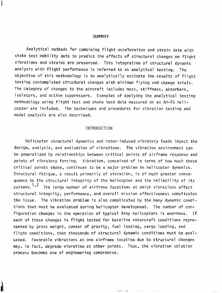
SUMMARY

Analytical methods for combining flight acceleration and strain data with

shake test mobility data to predict the effects of structural changes on flight

vibrations and strains are presented. This integration of structural dynamic

analysis with flight performance is referred to as analytical testing. The objective of this methodology is to analytically estimate the results of flight

testing contemplated structural changes with minimum flying and change trials.

The category of changes to the aircraft includes mass, stiffness, absorbers,

isolators, and active suppressors. Examples of applying the analytical testing

methodology using flight test and shake test data measured on an AH-1G heli-

copter are included. The techniques and procedures for vibration testing and

modal analysis are also described.

INTRODUCTION

Helicopter structural dynamics and rotor-induced vibratory loads impact the

design, analysis, and evaluation of vibrations. The vibration environment can

be generalized by relationships between critical points of airframe response and

points of vibratory forcing. Vibration, conceived of in terms of how much these

critical points shake, continues to be a major problem in helicopter dynamics.

Structural fatigue, a result primarily of vibration, is of much greater conse-

quence to the structural integrity of the helicopter and the reliability of its

systems. ly2 The large number of airframe locations at which vibrations affect

structural integrity, performance, and

the issue. The vibration problem is a

tions that must be evaluated during he

figuration changes in the operation of

each of these changes is flight tested

sented by gross weight, center of grav i

overall mission effectiveness complicates

so complicated by the many dynamic condi-

icopter development. The number of con-

typical Army helicopters is enormous. If

for baseline rotorcraft conditions repre-

ty, fuel loading, cargo loading, and

flight conditions, then thousands of structural dynamic conditions must be eval-

uated. Favorable vibrations at one airframe location due to structural changes

may, in fact, degrade vibration at other points. Thus, the vibration solution

process becomes one of engineering compromise.

Structural dynamics analysis has not proven to be one of the most useful

engineering tools in helicopter development.' As conventionally practiced, most helicopter vibration tests provide limited information for resolving

vibration issues. Helicopter flight vibration tests provide a direct measure

of the actual vibration environment while airframe ground vibration tests are

most often conducted to correlate analytical predictions of airframe resonances

and mode shapes. If there is reasonable agreement between analysis and test,

then confidence in the validity of the analysis is enhanced. However, if

reasonable agreement is not obtained, then an impasse results. Vibration prob-

lems are extremely difficult to quantify and have been solved by trial-and-error

ground and flight vibration testing.

The integration of structural dynamics analysis with flight performance,

herein referred to as analytical testing, appears to offer a practical method-

ology to the vibration solution process in helicopter development. This report

describes analytical methods for combining flight acceleration and strain data

with shake test mobility data to estimate the effects of contemplated changes

on aircraft vibrations and stresses for various flight conditions and maneuvers.

The category of changes to the aircraft includes external stores, weapons,

cargo, changes in structure or materials of structure, absorbers, isolators, or

active vibration suppressors. The objective of analytical testing methodology

is to analytically estimate the results of flight testing such changes with

minimum flying and change trials and to provide accurate and consistent dynamics

information for reduced cost and testing time.

The present investigation applied the analytical testing methodology in

conjunction with full-scale helicopter ground and flight test vibration data.

An AH-1G test vehicle was utilized in this project to provide ground vibration

data of realistic quality. Flight test data of the AH-1G was obtained from

another Army program on an as-available basis. The analytical testing examples

in this report use AH-1G data to illustrate possible generic applications of

the methodology. The authors do not suggest or imply applicability of these

examples to the AH-1G or any other specific helicopter. The applications des-

cribed herein were directed to the practical acquisition of helicopter vibra-

tion data for analytical testing and the possible utilization of the method.

2

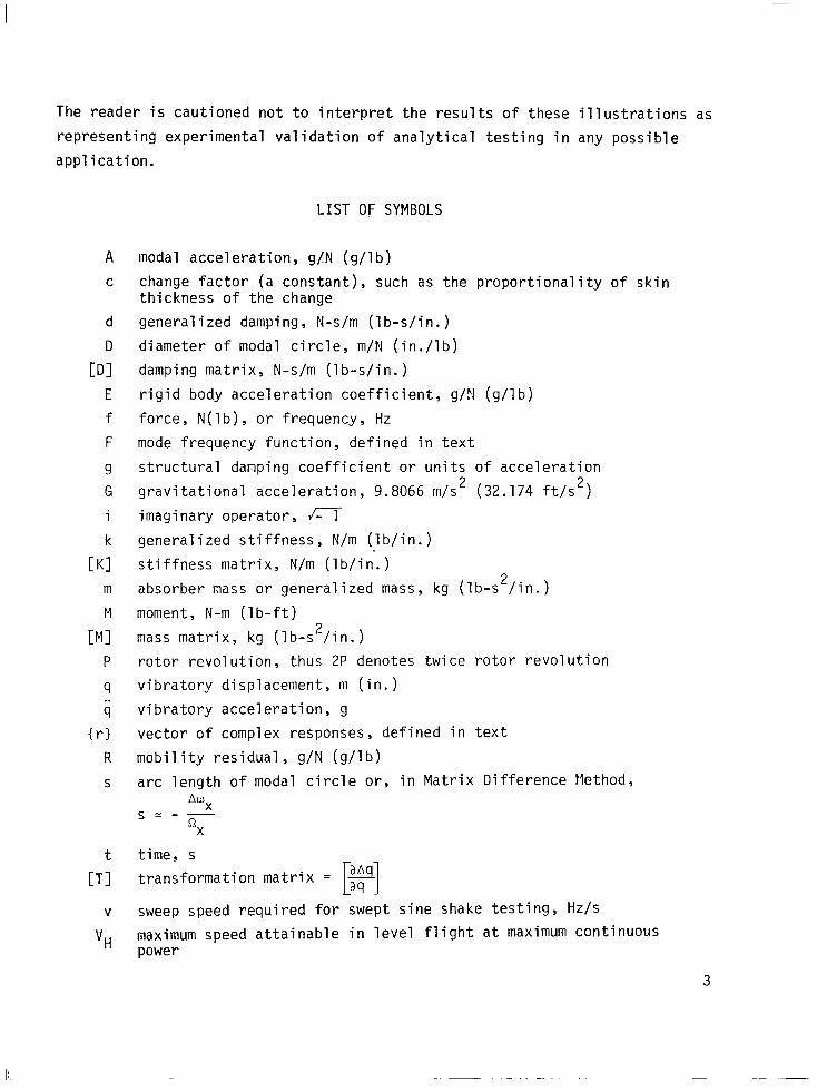
The reader is cautioned not to interpret the results of these illustrations as

representing experimental validation of analytical testing in any possible

application.

A

C

d

D

EDI

E

f

F

9 G

i

k

[Kl m

M

[Ml P

9

i

IrI

R

S

t

[J-l

V

vH

LIST OF SYMBOLS

modal acceleration, g/N (g/lb)

change factor (a constant), such as the proportionality of skin thickness of the change

generalized damping, N-s/m (lb-s/in.)

diameter of modal circle, m/N (in./lb)

damping matrix, N-s/m (lb-s/in.)

rigid body acceleration coefficient, g/N (g/lb)

force, N(lb), or frequency, Hz

mode frequency function, defined in text

structural damping coefficient or units of acceleration

gravitational acceleration, 9.8066 m/s2 (32.174 ft/s2)

imaginary operator, fl

generalized stiffness, N/m (lb/in.)

stiffness matrix, N/m (lb/in-.)

absorber mass or generalized mass, kg (lb-s2/in.)

moment, N-m (lb-ft)

mass matrix, kg (lb-s2/in.)

rotor revolution, thus 2P denotes twice rotor revolution

vibratory displacement, m (in.)

vibratory acceleration, g

vector of complex responses, defined in text

mobility residual, g/N (g/lb)

arc length of modal circle or, in Matrix Difference Method,

AwX se----- “X

time, s

transformation matrix = T [ 1 sweep speed required for swept sine shake testing, Hz/s

maximum speed attainable in level flight at maximum continuous power

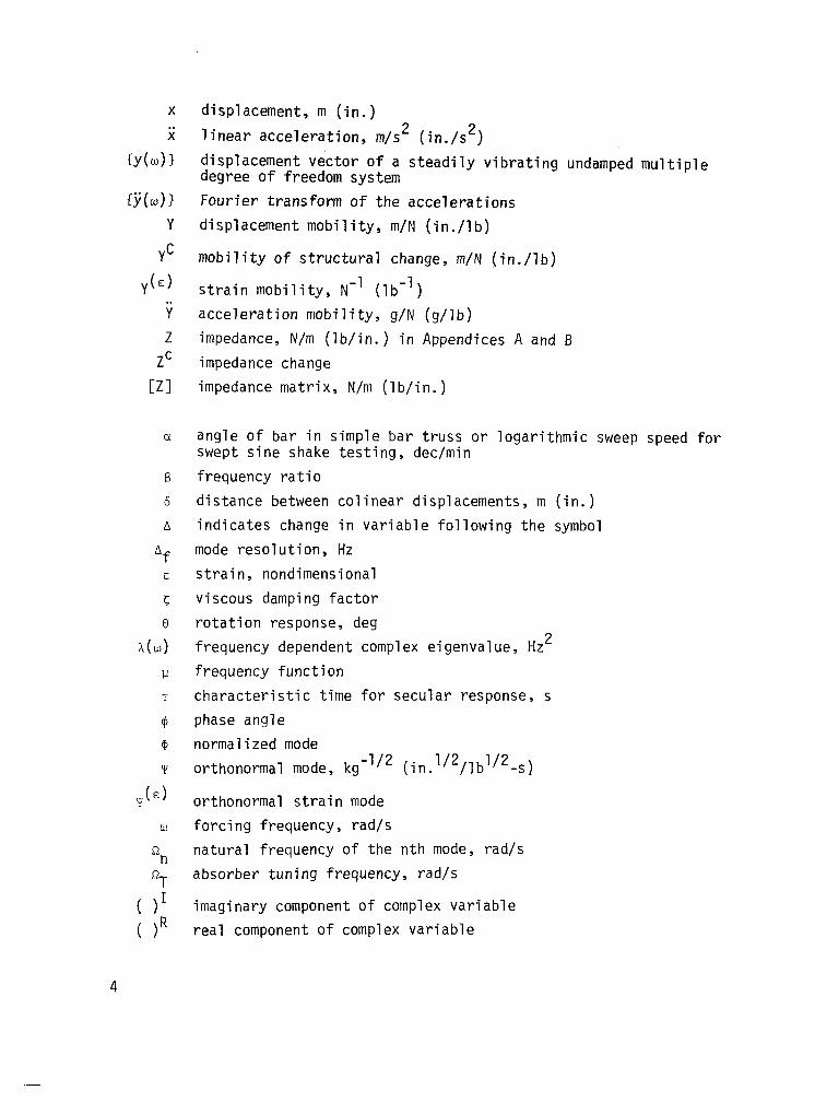
X displacement, m (in.)

i linear acceleration, m/s2 (in./s2)

{Y(dl displacement vector of a steadily vibrating undamped multiple degree of freedom system

ij;(Ld> 1 Fourier transform of the accelerations

Y displacement mobility, m/N (in./lb)

YC mobility of structural change, m/N (in./lb)

y(E) strain mobility, N-' (lb-')

;i acceleration mobility, g/N (g/lb)

Z impedance, N/m (lb/in.) in Appendices A and B

ZC impedance change

PI impedance matrix, N/m (lb/in.)

CY. angle of bar in simple bar truss or logarithmic sweep speed for swept sine shake testing, dec/min

frequency ratio

distance between colinear displacements, m (in.)

indicates change in variable following the symbol

mode resolution, Hz

strain, nondimensional

viscous damping factor

rotation response, deg

frequency dependent complex eigenvalue, Hz2

frequency function

characteristic time for secular response, s

phase angle

normalized mode

orthonormal mode, kg -l/2 (in 1'2/lb1'2-s) .

&I orthonormal strain mode

w forcing frequency, rad/s

'n natural frequency of the nth mode, rad/s

"T absorber tuning frequency, rad/s

( )I imaginary component of complex variable

( lR real component of complex variable

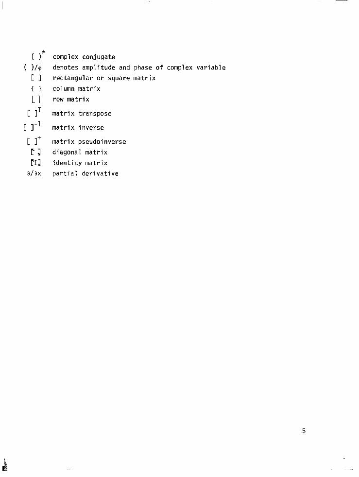
( I* complex conjugate

( )/$I denotes amplitude and phase of complex variable

[ 1 rectangular or square matrix

c 1 column matrix

Ll row matrix

c IT matrix transpose

c 1-l matrix inverse

II 1+ matrix pseudoinverse

C J diagonal matrix

CIiJ identity matrix

a/ax partial derivative

5

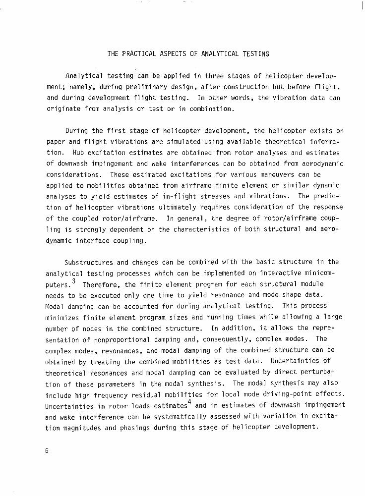
THE PRACTICAL ASPECTS OF ANALYTICAL TESTING

Analytical testing can be applied in three stages of helicopter develop-

ment; namely, during preliminary design, after construction but before flight,

and during development flight testing. In other words, the vibration data can

originate from analysis or test or in combination.

During the first stage of helicopter development, the helicopter exists on

paper and flight vibrations are simulated using available theoretical informa-

tion. Hub excitation estimates are obtained from rotor analyses and estimates

of downwash impingement and wake interferences can be obtained from aerodynamic

considerations. These estimated excitations for various maneuvers can be

applied to mobilities obtained from airframe finite element or similar dynamic

analyses to yield estimates of in-flight stresses and vibrations. The predic-

tion of helicopter vibrations ultimately requires consideration of the response

of the coupled rotor/airframe. In general, the degree of rotor/airframe coup-

ling is strongly dependent on the characteristics of both structural and aero-

dynamic interface coupling.

Substructures and changes can be combined with the basic structure in the

analytical testing processes which can be implemented on interactive minicom-

puters. 3 Therefore, the finite element program for each structural module

needs to be executed only one time to yield resonance and mode shape data.

Modal damping can be accounted for during analytical testing. This process

minimizes finite element program sizes and running times while allowing a large

number of nodes in ttie combined structure. In addition, it allows the repre-

sentation of nonproportional damping and, consequently, complex modes. The

complex modes, resonances, and modal damping of the combined structure can be

obtained by treating the combined mobilities as test data. Uncertainties of

theoretical resonances and modal damping can be evaluated by direct perturba-

tion of these parameters in the modal synthesis. The modal synthesis may also

include high frequency residual mobilities for local mode driving-point effects.

Uncertainties in rotor loads estimates4 and in estimates of downwash impingement

and wake interference can be systematically assessed with variation in excita-

tion magnitudes and phasings during this stage of helicopter development.

6

In the second stage of helicopter development, after construction but

before flight, a shake test aircraft should be available. This non-flying

shake test aircraft would be used for analytical testing of changes, ground

flying for fatigue evaluation,5 and analysis of accidents. In this stage, shake testing data can be used to refine the existing finite element

models. 6,7,8 Mobilities from finite element models of substructure can be com-

bined with mobilities from tests of other subsystems to obtain total system

mobilities, resonances, modal damping, and complex modes. In general, the fuselage system mobilities and the mobilities of complex components, such as

engines, may be obtained through shake testing while mobilities of contemplated

changes, flexible portions of the airframe, and low mass structural appendages

would be obtained through finite element modeling. This separation between

finite element modeling and shake testing for analytical testing purposes

offers optimum utilization of finite element analysis and modal analysis shake

testing. The major accomplishment in this stage is the application of refined

mobilities for identifying favorable structural changes to adjust airframe

resonances and nodes. Theoretical estimates of the vibratory loads are com-

bined with these mobilities to estimate changes in vibrations and stresses.

During the third stage of helicopter development, analytical testing uses

only ground and flight vibration data to estimate changes in flight responses

caused by structural and configuration changes. As the flight envelope of the

prototype aircraft is expanded, flight vibration data can be applied directly

since the theoretical estimates of external excitations are no longer needed.

Anticipated changes such as stores, weapons, cargo, and structure can be exam-

ined for flight effects on vibrations and stresses before actual flight. Know-

ledge of the number, types, or locations of the external excitations is not

required. The only flight data necessary are accelerations and strains mea-

sured during the initial flight tests.

ANALYTICAL TESTING THEORY

The matrix equations of motion for a damped linear structure can be gener-

alized in the frequency domain as

[K] - w2 CM] + i [D(U)] 1

{q1 = IfI (7)

where [K], [M], and [D(U)] are Nth ordered stiffness, mass, and damping matrices,

respectively. The matrix terms on the lefthand side of equation (1) define the

displacement impedance matrix, [Z], or

lIZI IqI = If-1 (2)

The dynamic responses can thus be characterized by the simple matrix equation

given by

where

(q1 = PI If1

[Y] = [z]-'

(3)

(4)

and the variables in equation (3) are complex valued and frequency dependent.

The matrix [Y] is the transfer function which relates the input excitations,

IfI, to the output responses, {q). If the response vector is displacement,

velocity, or acceleration, then the transfer function is defined as the displace-

ment, velocity, or acceleration mobility, respectively. Compliance, mobility,

and inertance are sometimes used in the literature to define the corresponding

displacement, velocity, and acceleration mobilities.

Types of Mobilities

Mobilities are defined as partial derivatives of response with respect to

excitation in the frequency domain. In general, there are two separate types

of mobilities used in analytical testing which can be distinguished by consid-

ering the nature of the response and the excitation.

8

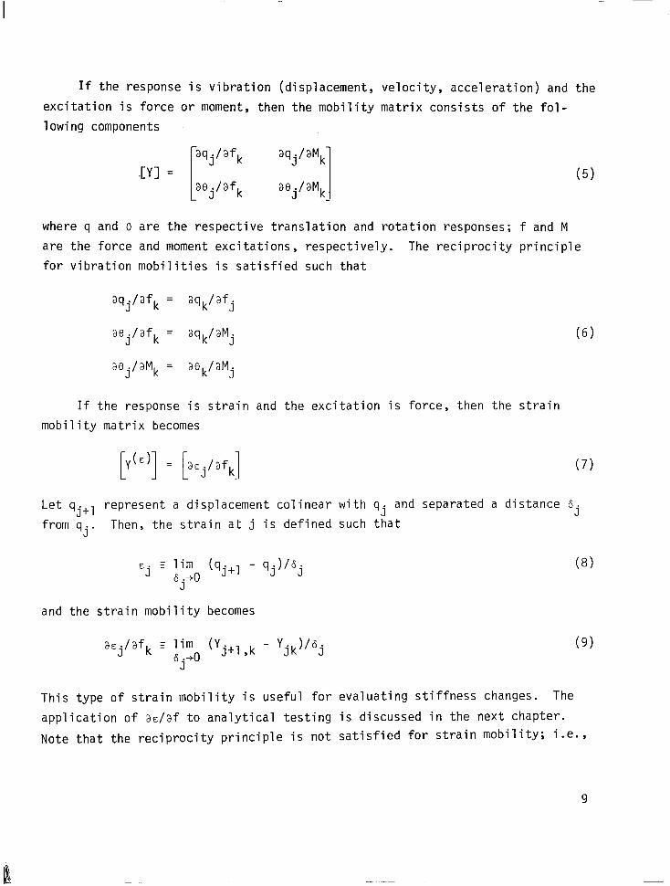
If the response is vibration (displacement, velocity, acceleration) and the

excitation is force or moment, then the mobility matrix consists of the fol-

lowing components

aqj/afk

i

Wj/aMk .[Y] =

aej/afk aej/aMk 1 (5)

where q and 8 are the respective translation and rotation responses; f and M

are the force and moment excitations, respectively. The reciprocity principle

for vibration mobilities is satisfied such that

aqj/afk = aqk/afj

aej/afk = aqk/aM. J

aaj/aMk = aek/aMj

If the response is strain and the excitation is force, then the strain

mobility matrix becomes

p(')] = [acj/afk]

(6)

(7)

Let 9j+] represent a displacement colinear with qj and separated a distance Aj

from qj. Then, the strain at j is defined such that

E. J

= lim (qj+l - qj)j6j aj"

and the strain mobility becomes

aEj/afk q lim (Yj+l k - Yjk)/Gj aj+o ’

(8)

(9)

This type of strain mobility is useful for evaluating stiffness changes. The

application of ae/af to analytical testing is discussed in the next chapter.

Note that the reciprocity principle is not satisfied for strain mobility; i.e.,

9

a&j/afk # a&k/af. J (‘0)

Analytical Testing Equations

The solution to helicopter vibration problems consists, in part, of pre-

dicting and confirming the flight vibration or strain effects of dynamic changes

in the airframe, on the rotor, or at the rotor/airframe interface. Let {q1 and {eI represent the baseline vibration and strain, respectively. Then, (q'} and {E'}

represent the change in baseline vibration and strain due to a dynamic change.

In theory, {q') and CE') can result from either a change in the mobility matrix

or a change in the vibratory loading. The basic analytical testing method con-

siders changes in the mobility matrix which can be synthesized by discrete as

well as multiple and distributed dynamic impedance adjustments. The category

of impedance changes that can be accommodated includes mass, stiffness, absor-

bers, isolators, and active suppressors. As shown in Appendix A, the matrix

equation for determining the change in baseline vibration for a general multi-

dimensional impedance change is

lq’l = Cql - YqI 1.1 r

[YIi + yII]- 1 i I q1 (1’)

where YI; is defined from the impedance change. The mobilities YqI and YII

represent transfer functions for the baseline structure at the change interface

and do not include the effects of the impedance change. In other words, for a

properly modeled impedance change, the effects on flight vibrations are evalu-

ated without incorporating the change in the baseline structure. Therefore,

only one NASTRAN or similar dynamic analysis is required to implement equa-

tion (11). If changes in strain, as opposed to vibration, are considered, then

equation (11) becomes

lE’1 = C&l - cy6;‘] [yr: + yII]-’ {qr) c.721

In summary, the changed flight responses (vibration or strain) are charact-

erized by the dynamics of the impedance change, the baseline flight responses,

and the baseline mobility responses. The operational equations can be used with

either theoretically derived vibration and strain data or ground and flight

10

vibration and strain measurements. In the next chapter , equations (11) and (12) are considered for examining mass, stiffness, and absorber changes to illustrate

the analytical testing methodology.

Limitations of the Method

Basic to the analytical testing method are the assumptions that the struc-

ture is linear and that changes to the structure do not change the external

loadings. These conditions are only approximated in an actual helicopter

flight. The airframe is not a linear system , as shake tests of the AH-1G showed, but it appears that it can be represented as linear for most practical

engineering purposes.

The second assumption is a workable approximation under some conditions of

change and not under others. It is important to note that the mobilities used

in analytical testing must be physically realizable and consistent for any

driving-point. Mobilities obtained using a lumped mass representation of the

rotor at the hub violate this requirement but the practical effect of the viola-

tion is not known. Ideally, the mobiljties of the airframe would contain the

dynamic effects of a rotating rotor in a vacuum and this might be approximated

by coupling theoretical rotor mobilities with shake test airframe mobilities in

the analytical testing equation, except that the partial derivatives of in-plane

hub motions with respect to in-plane hub forces have periodic coefficients. It

is not analytically difficult to handle this problem, and therefore remove this

particular limitation, but the practicality of doing so has not been estab-

lished. The effect on change estimates of airframe mobilities without a

rotating rotor in a vacuum is discussed in Appendix B.

The basic analytical testing equation is of the form

{q'l = Iq1 - [A] Ir) (-73)

where q is the vector of complex motions (vibrations or strains) on the air-

frame measured in flight without a structural change, r is the vector of com-

plex motions measured in flight at the coordinates of the structural change,

q' is the vector of complex flight motions that result from the change and A is

11

a matrix function of measured airframe mobilities and mobilities of the struc-

tural change. If the structural change has negligible effect on the structural

dynamics of the helicopter, the A matrix is nearly null and Ar is negligible;

resulting flight vibrations and strains are virtually unchanged. If, on the other hand, the structural change has a significant effect on the dynamics such

that the absolute values of the Ar terms are much greater than the absolute

values of the q terms, then the change will make the flight vibrations and

strains much higher. It is seen, therefore, that analytical testing is least

sensitive to errors in mobilities or modeling of the structural change when:

(1) the structural change has negligible effect on flight vibrations and strains;

and (2) the structural change results in much higher flight vibrations and

strains.

The practical consequence is that one does not need high precision mobili-

ties or change modeling to filter out quite rapidly those structural changes

which either do not significantly change flight vibrations or strains or those

structural changes which will significantly worsen flight vibrations or strains.

Since most changes contemplated in the life cycle of a military helicopter are

for mission improvement, not dynamics or stress improvement, there is an

obvious value in using approximate but not precise structural dynamics data to

identify those changes which are likely to create serious flight structural

problems before proceeding with flight testing the changes or with more expen-

sive and more precise measures of analysis and test.

APPLICATIONS OF ANALYTICAL TESTING

The following numerical illustrations of the analytical testing methodol-

ogy utilize ground and flight vibration data obtained from an Army AH-1G test

vehicle. The types of dynamic changes which are considered include mass, stiff-

ness, absorber, and active suppressors. Except for the mass change example,

the analytical testing illustrations are hypothetical. In addition, these

results do not suggest applicability to the AH-1G or any specific helicopter.

12

Test Vehicle and Test Conditions

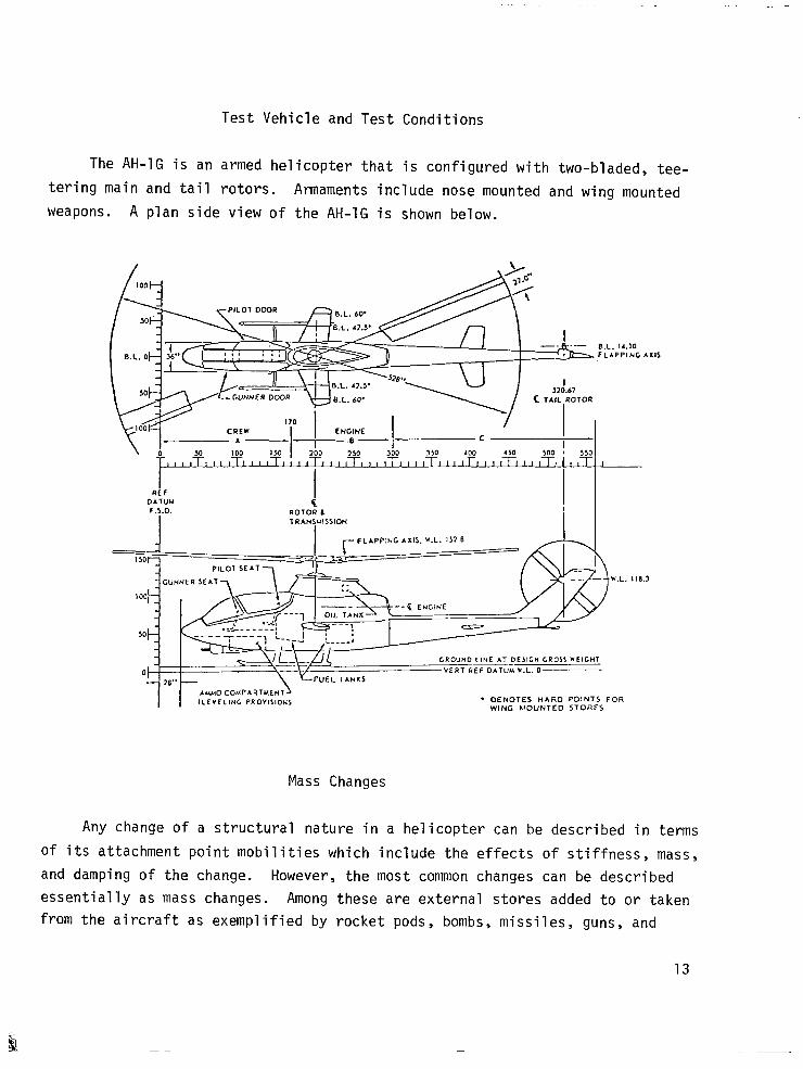
The AH-1G is an armed helicopter that is configured with two-bladed, tee-

tering main and tail rotors. Armaments include nose mounted and wing mounted

weapons. A plan side view of the AH-1G is shown below.

Mass Changes

Any change of a structural nature in a helicopter can be described in terms

of its attachment point mobilities which include the effects of stiffness, mass,

and damping of the change. However, the most common changes can be described

essentially as mass changes. Among these are external stores added to or taken from the aircraft as exemplified by rocket pods, bombs, missiles, guns, and

13

external fuel. There is often an extremely large number of possible combina-

tions of external stores on helicopters because of the variety of missions.

Cargo and transport helicopters have many variations in payload of a mass

change nature. There are mass changes from fuel burn-off, depletion,of ammu-

nition, and firing of rockets or missiles.

In the continuing development of a helicopter it would be expeditious to

predict the effects of flight stresses and vibration of such changes so that

problem areas can be anticipated, engineering judgments can be made, and cor-

rective action prepared with minimum trial-and-error testing. Allowing for

flight data scatter, the engineer would make such predictions at several criti-

cal locations with analytical testing for critical classes of maneuvers. It is

impractical to attempt precise predictions for every possible airspeed, gross

weight, c.g. location, yaw rate, pitch rate, roll rate, power setting, air tem-

perature, wind condition, altitude, etc., and for all the locations of interest

on the helicopter. In a well developed helicopter analytical testing would be

used for major changes, such as the contemplated addition of rocket pods, but

in a helicopter in the early stages of development analytical testing would be

applied to a wider variety of mass changes to aid in identifying possible

problems.

A Flight Example for Mass Changes

The AH-1G is used 'to illustrate the analytical testing methodology. Con-

sider the hypothetical situation of an AH-1G which had never flown with rocket

pods. An addition of rocket pods weighing 181 kg (400 lb) each to the outboard

wing station is contemplated. This represents a 9.4 percent increase in the

gross weight of the helicopter. The predictions are made from the clean con-

figuration for classes of maneuvers without accounting for additional drag,

fuel burnoff, or other causes of possible changes in external aerodynamic

loading.

The following flight acceleration data were taken on an as-available basis

from another project. No strain data were available. The clean configuration,

without rocket pods, had a take-off gross weight of 3830 kg (8465 lb) and was

14

flown in ground winds of 5 to 7 knots, Outside Air Temperature (OAT) of 10°C

(50°F) and 766 mm (30.17 in.) Hg barometric pressure. The flights with the

rocket pods were made at 4106 kg (9075 lb) take-off gross weight with ground

winds of 3 to 5 knots, OAT of 20°C (68°F) and 754 mm (29.68 in.) Hg barometric

pressure. The c.g. was at FS 196.3 in both flights. Power and control settings

were not necessarily matched in the flights. Data were analyzed for the condi-

tion of highest peak-to-peak vibration of a set of selected. points, differing

from flight to flight, in each class of flight condition with a harmonic anal-

ysis over five to eight rotor revolutions. Except for the unavailability of

strains, this situation is representative of practical application of analy-

tical testing.

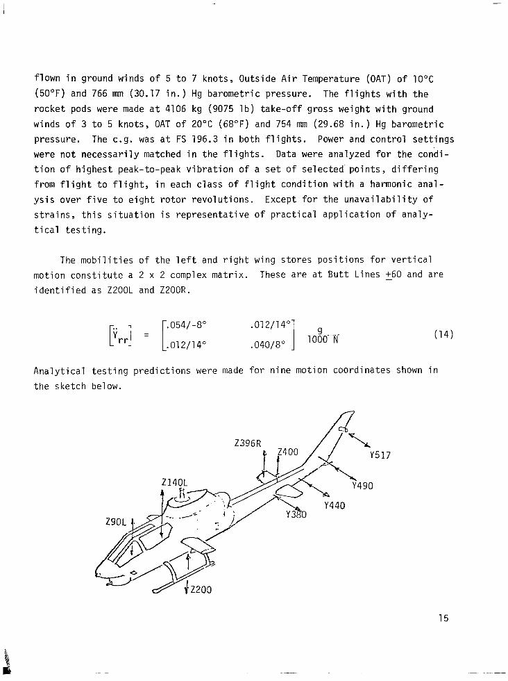
The mobilities of the left and right wing stores positions for vertical

motion constitute a 2 x 2 complex matrix. These are at Butt Lines 560 and are

identified as Z2OOL and ZZOOR.

r.. i r.O54/-8" .012/14"

l'rd = 1.012, 14" .040/8" I lo:0 N (14)

were made for nine motion coordinates shown in Analytical testing predictions

the sketch below.

15

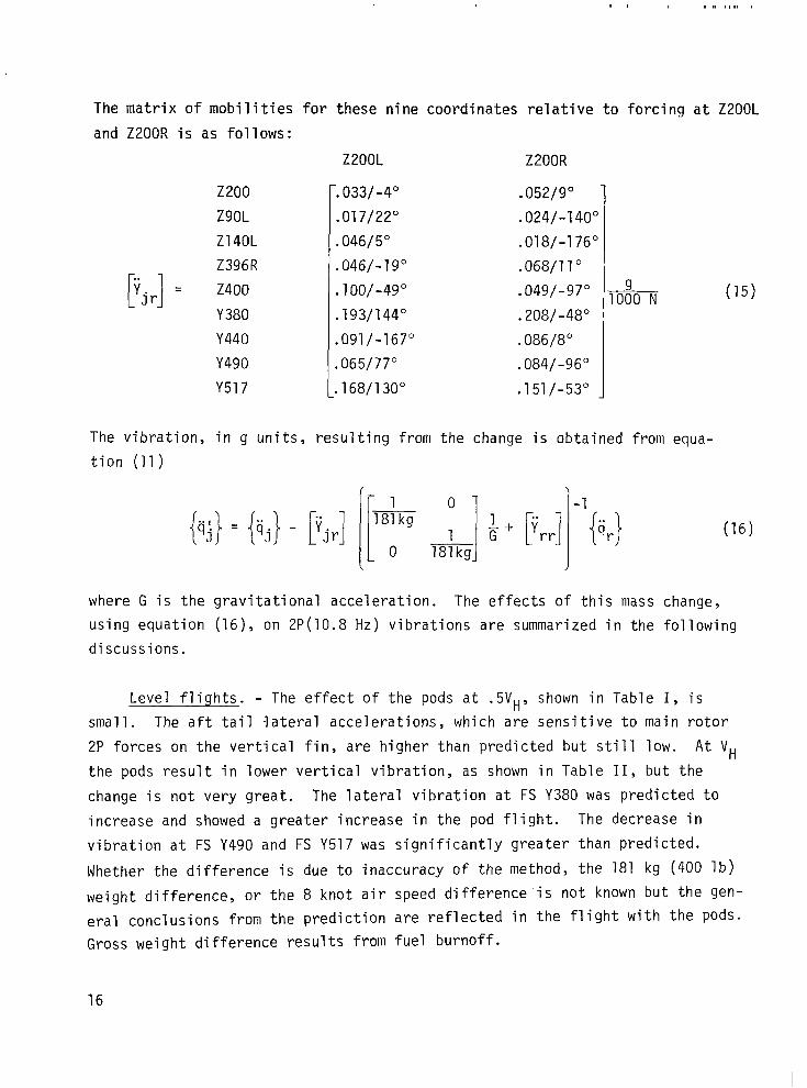
The matrix of mobilities for these nine coordinates relative to forcing at Z2OOL

and Z200R is as follows:

i

Yjr

2200

Z9OL

Zl4OL

Z396R

I = . 2400

Y380

Y440

Y490

Y517

Z200L

.033/-4O

.017/22O

.046/5"

.046/-19"

.lOO/-49"

.193/144"

.091/-167"

,065/77"

#168/130"

Z200R

.052/9”

.024/-140"

.018/-176"

.068/11"

.049/-97O

.208/-48O

.086/8"

.084/-96'

.151/-53O

lOi0 N (15)

The vibration, in g units, resulting from the change is obtained from equa-

tion (11)

(16)

where G is the gravitational acceleration. The effects of this mass change,

using equation (16), on 2P(lO.8 Hz) vibrations are summarized in the following

discussions.

Level flights. - The effect of the pods at .5VH, shown in Table I, is

small. The aft tail lateral accelerations, which are sensitive to main rotor

2P forces on the vertical fin, are higher than predicted but still low. At VH

the pods result in lower vertical vibration, as shown in Table II, but the

change is not very great. The lateral vibration at FS Y380 was predicted to

increase and showed a greater increase in the pod flight. The decrease in

vibration at FS Y490 and FS Y517 was significantly greater than predicted.

Whether the difference is due to inaccuracy of the method, the 181 kg (400 lb)

weight difference, or the 8 knot air speed difference'is not known but the gen-

eral conclusions from the prediction are reflected in the flight with the pods.

Gross weight difference results from fuel burnoff.

16

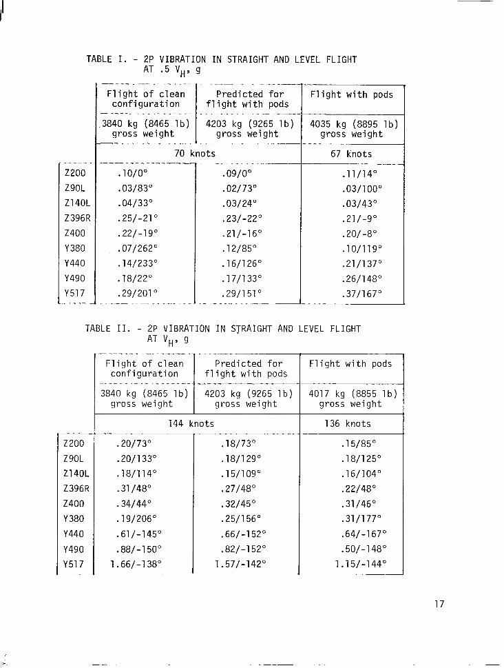
TABLE I. - 2P VIBRATION IN STRAIGHT AND LEVEL FLIGHT AT .5 VH, g

_----. 2200

Z90L

Zl4OL

Z396R

2400

Y380

Y440

Y490

Y517 .-- - _

- - -- -- _ - -~- -.-- - . .-~_- Predicted for

configuration flight with pods - _.~-~_-. . ,_=_-

3840 kg (8465 lb) 4203 kg (9265 lb) gross weight gross weight

--- ..-_~-_-. - --_-~_-_~_ 70 knots

---- _-- _~ -_____ .10/O"

.03/83O

.04/33"

.25/-21"

.22/-19O

.07/262O

.14/233"

.18/22O

.29/201" . -- ..-- _ - --- ~--

.09/O”

.02/73'

.03/24"

.23/-22"

.21/-16O

.12/85O

.16/126"

.17/133"

.29/151" _ ._ .----

Flight with pods

4035 kg (8895 lb) gross weight

67 knots

.11/14O

.03/100°

.03/43"

.21/-go

.20/-8"

.lo/llg"

.21/137"

.26/148'

.37/167"

TABLE II. - 2P VIBRATION IN STRAIGHT AND LEVEL FLIGHT AT v,,' 9

2200

Z9OL

Zl4OL

Z396R

2400

Y380

Y440

Y490

Y517

.20/73O

.20/133"

.18/114"

.31/48O

.34/44O

.19/206"

.61/-145'

.88/-150"

1.66/-138"

.18/73"

.18/129"

.15/109"

.27/48O

.32/45"

.25/156"

.66/-152"

.82/-152"

1.57/-142"

Flight with pods

4017 kg (8855 lb) gross weight

136 knots

.15/85O

.18/125"

.16/104='

.22/48"

.31/46"

.31/177O

.64/-167O

.50/-148"

1.15/-144"

17

Gunnery runs. - The data for the flight of the clean aircraft were not

necessarily taken for a portion of the rolling pullout comparable to that for

which those data were taken on the flight with the pods. From the prediction

of the effects of the pods, shown in Table III, the pods have little effect on

the vibration at some locations and cause a decrease in the vibration at others

in a high load factor rolling pullout to the left. The pod flight data leads

to the same conclusion. The same situation pertains in a rolling pullout to

the right, shown in Table IV. In this case the predictions for FS Z396R and

FS Y517 showed reductions that were not seen in the pod flight as did the pre-

diction for FS Y380 in Table III. However, considering the nature of the data

samples, the conclusion of the prediction is reflected in the pod flight.

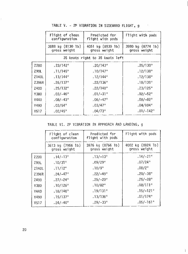
Sideward flight and landing. - The flight data in Table V are samples

taken from sideward flight to the right to 35 knots with reversal and sideward

flight to the left to 35 knots. There is no significant change in vibration

due to the pods in sideward flight or in approach and landing. The phase angles

of the data at very low g-levels, determined from harmonic analysis, are highly

variable. In approach and landing with pods, Table VI, the data sample shows

low vibration at FS 490 and FS 517, fin stations of large vibration scatter,

and is most likely the result of the time sample chosen.

18

TABLE III. - 2P VIBRATION IN ROLLING PULLOUT TO LEFT, g

2200

Z9OL

Zl4OL

Z396R

2400

Y380

Y440

Y490

Y517

2200

Z9OL

Zl40L

Z396R

2400

Y380

Y440

Y490

Y517

Flight of clean Predicted for configuration flight with pods

3645 kg (8035 lb) 4130 kg (9105 lb) gross weight gross weight

187 knots 1.42 g load factor

.53/85"

.46/118"

.47/105"

.52/73'

.94/68"

.50/-126"

1.28/-115"

1.27/-116"

1.82/-91"

.52/89”

.42/117'

.42/103'

.42/75='

.83/70"

.32/-158"

1.25/-120"

1.19/-114"

1.60/-89"

I

+

Flight with pods

3966 kg (8744 lb) gross weight

186 knots 1.52 g load factor

.58/84"

.42/116"

.40/104O

.54/76O

.79/66'

.52/-157"

1.04/-141"

.93/-121°

1.59/-97"

TABLE IV. - 2P VIBRATION IN ROLLING PULLOUT TO RIGHT, g

164 to 128 knots 1.78 to 1.5 g load factor

.36/84"

.49/129"

.43/115"

.33/55"

.82/61"

.47/-121"

.97/-114"

.71/-121"

.85/-106"

.32/85"

.44/128"

.37/113"

.26/56"

.72/61"

.24/193"

.94/-123"

.61/-116"

.58/-107"

Flight with pods

4042 kg (8909 lb) gross weight

162 knots 1.23 g load factor

.24/79”

.31/117"

.31/106"

.47/71°

.63/60°

.24/-167"

.79/-158"

.47/-144O

.85/-123"

19

2200

Z9OL

Zl4OL

Z396R

2400

Y380

Y440

Y490

Y517

2200

Z90L

Zl4OL

Z396R

2400

Y380

Y440

Y490

Y517

TABLE V. - 2P VIBRATION IN SIDEWARD FLIGHT, g

~

35 knots right to 35 knots left

.23/142O

.11/145"

.13/144"

.26/137"

.25/132"

.03/-46"

.08/-43"

.03/54"

.02/45'

.20/143"

.10/147"

.12/144O

.22/136"

.22/140"

.Ol/-31"

.06/-47"

.03/47"

.04/73"

.25/130"

.12/138O

.12/138O

.18/131'

.23/125'

.02/-52O

.08/-82O

.04/104"

.Ol/-142'

TABLE VI. 2P VIBRATION IN APPROACH AND LANDING, g

Flight of clean configuration

3613 kg (7966 lb) gross weight

.14/-13"

.10/31"

.ll/i2"

.24/-47"

.27/-24"

.10/126"

.18/140"

.15/137"

.24/-40"

Predicted for flight with pods

3976 kg (8766 lb) gross weight

.13/-13"

.09/29"

.10/9"

.22/-49"

.25/-20"

.10/82"

.19/131"

.13/136"

.29/-33"

Flight with pods

4002 kg (8824 lb) gross weight

.14/-21°

.07/24"

.08/2"

.20/-38"

.25/-28"

.08/lll"

.15/-121"

.01/174O

.05/-161"

20

Vibration Absorber Changes

All major helicopter manufacturers have used conventional spring-mass

vibration absorbers with varying degrees of success. Except for in-plane cen-

trifugal hub absorbers which are used to cancel (N-1)P and (N+l)P shears in the

rotating system of helicopters, absorbers are customarily tuned to be coinci-

dent with the excitation frequency and placed at the airframe location where

vibration reduction is needed. In limited applications, airframe absorbers

have been remotely placed from points where low vibration is desired. The

remote absorber has the advantage of providing vibration reduction at locations

where conventional airframe absorbers are physically impractical. These remote

absorbers have been trial-and-error tuned to be somewhat off resonance to

achieve optimum vibration reduction.

Airspeed, gross weight, and center of gravity variations alter the rela-

tive magnitudes and phasings of airframe responses, thus absorber effectiveness

varies. There are two situations in which the effects of absorbers are indepen-

dent of the airspeed and flight maneuver of the helicopter. First, is the

extreme situation with absorbers coincident to each vectorial coordinate of

external forces and moments acting on the helicopter. In this case, the entire

airframe has virtually zero vibration at all airspeeds and in all maneuvers.

The second situation is at the attachment point of the absorbers along the

absorber direction. Clearly, the dynamicist must consider the flight effects

of a limited number of absorbers at airframe locations remote from the

absorbers.

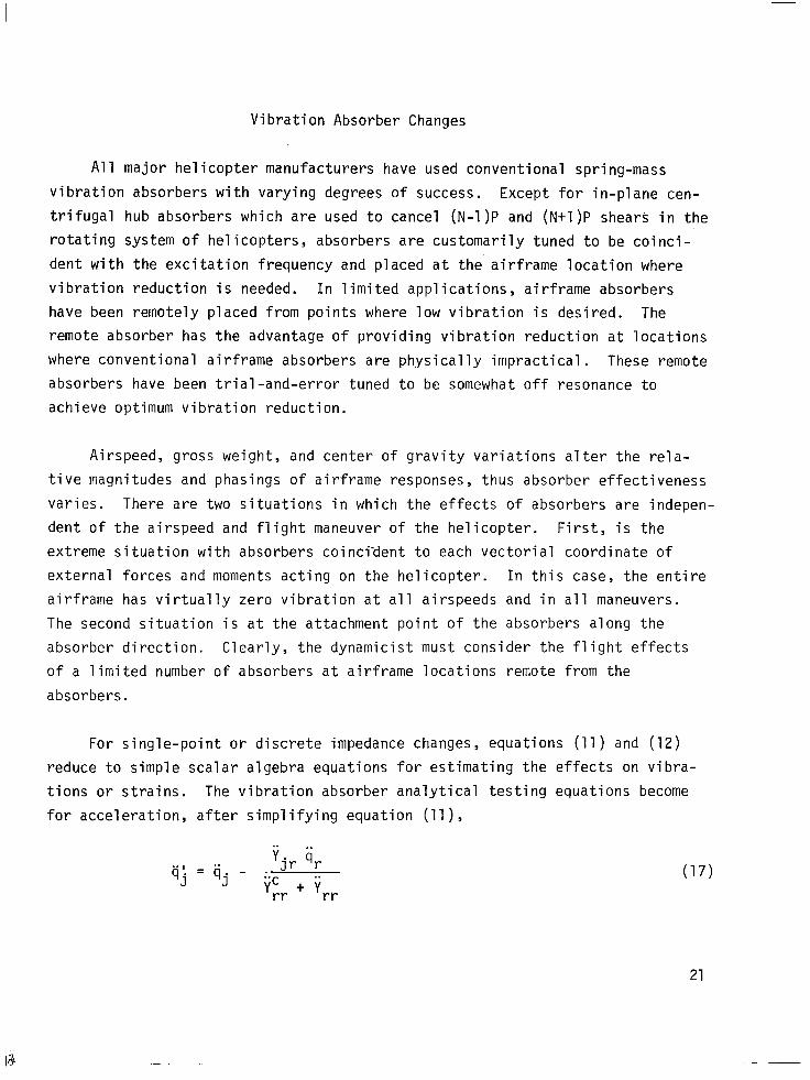
For single-point or discrete impedance changes, equations (11) and (12)

reduce to simple scalar algebra equations for estimating the effects on vibra-

tions or strains. The vibration absorber analytical testing equations become

for acceleration, after simplifying equation (11),

;i i e-1 = --

qj qj - YC

jr r

rr + 'rr

(17)

21

and, for strain, after simplifying equation (12)

y (4 q jr r

Ej = Ej - ;i c

rr + 'r-r

08)

where ?,.F is the unrestrained driving-point acceleration mobility of the absor-

ber at its attachment point r. For a structurally damped absorber, the unre-

strained driving-point acceleration mobility is

;i c = 1- T+ig u2/Q2

rr m(l+ig) (19)

where aT is the tuning frequency, m is the absorber mass, and g is the non-

dimensional structural damping coefficient. Similarly, with viscous damping

. . yc=

l- u2/Q2 T + i2yw/RT

rr m(l+i2&nT) (20)

where 5 is the viscous damping factor. As equations (17) and (18) show, the

required absorber weight, tuning frequency (not necessarily equal to the excita-

tion frequency), and damping (not necessarily zero) for minimum vibration or

strain along the motion coordinate j are functions of the flight vibration at r,

the flight vibration or strain at j, the r-j mobility, and the r-r mobility. A

vibration absorber can be designed to minimize both vibrations and strains. For

vibratory strains the required r-j mobility is defined as the strain mobility.

Vibration attenuation is a fundamental objective in dynamics and equa-

tion (17) can be written in a slightly different form as

;i q/s j = 1.0 -

jr iirliij

Y --"r t i; rr

(21)

The effects of tuning and damping on vibration at j can be examined by plotting

the absolute value of (qj/qj) versus the tuning ratio, nT/w, for fixed ValUeS

of damping. Interactive computer graphics offer the capability to investigate

the effects at various critical airframe locations to select the tuning fre-

quency for the optimum overall effect. A weighting factor can be assigned to

22

li'/ql for each station and one composite curve can be displayed for many

stations.

Conventional absorbers are analyzed with regard to vibration at the absor-

ber attachment point r. If j replaces r in equation (21), then the absorber

transmissibility becomes

or, after substituting for y",, in equation (19),

1 - U2/Q2 T + ig

;il';ir = 2 1 - %t YFrrn - ;iFrmg t i

I ;iFrrn + mg;jFr t g

"T 1

(22)

(23)

The percentage reduction of vibration at the absorber attachment point is, of

course, independent of the flight vibration. A conventional absorber with zero

damping produces zero vibration when ?Fr is zero or when the tuning frequency

coincides with the excitation frequency. When the forcing frequency equals the

tuning frequency, equation (23) gives

(24)

Thus, for a given absorber damping the attachment point vibration ratio is

inversely proportional to the absorber mass.

The imaginary part of the helicopter driving-point acceleration mobilities

is necessarily positive, but the real part may be either positive or negative.

Because helicopter structures do not have proportional damping the modes are,

in general, complex and, even in the vicinity of a well separated mode with a

high rr modal acceleration (residue), the real part of the driving-point mobil-

ity is not necessarily smaller just below resonance than just above a resonance

23

as in structures with classical modes. For structures with classical modes,

the signs of the real parts of the driving-point mobilities may be the same

just above and just below a resonance, due to coupling of other modes, and

that sign may be positive or negative. Therefore, the resonance introduced

by the addition of the absorber may occur above or below the driving-point

antiresonant frequency created by the absorber. Because the driving-point

mobility is a function of frequency it is necessary to examine equation (22)

over a frequency spectrum to determine the absorber bandwidth, that is, the

change in resultant vibration with variation in excitation frequency or rotor

speed.

As seen from equation (24), the vibration ratio at the attachment point

is, for small damping, directly proportional to the damping. This leads to the

misconception that minimal absorber damping is desirable regardless of the loca-

tion of the absorber and the point of concern on the helicopter.

Obtaining zero vibration. - In equation (21) let (J? be zero. Then,

The absorber mobility required for zero vibration along the j motion coordinate

is a function of the in-flight vibration of the motion coordinate j and that of

the absorber, r. The complex 4,/i, ratio will usually be different for each

flight condition and zero vibration at j from an absorber at r is dependent on

the flight condition. Since the driving-point imaginary acceleration mobility

must be positive, it is necessary but not sufficient for the imaginary part of

the right hand side of equation (25) to be positive for zero vibration.

Through control of absorber damping zero vibration at a desired point can be

achieved in any one flight condition only under certain circumstances.

24

Examples of Absorber Analysis

The following examples are presented to illustrate the applicability of

analytical testing for examining the effects of absorbers on AH-1G airframe

vibrations. The absorber is a simple spring-mass device with hysteretic damping

as discussed for equation (19). Equations (21) and (22) are used to determine

the performance of the absorber at critical points on the airframe for several

representative flight conditions.

Absorber at nose. - This example considers the effects on vertical vibra-

tion at the gunner's left (FS Z9OL) and at the horizontal stabilizer (FS 2400).

A vertical absorber, weighing 13.61 kg (30 lb), is located at the nose (FS 250)

of the AH-1G as shown in the sketch below.

The acceleration mobilities which were measured during the ground vibra-

tion test are

.lOO g/l000 N (.044 g/l00 lb)/lO"

.09 g/l000 N (.040 g/l00 lb)/8"

.232 g/l000 N (-103 g/l00 lb)/l23=' (26)

25

The vibrations measured in flight are shown in Table VII. The driving-

point mobility at FS 250 is nearly the same as the transfer mobility between

250 and Z9OL and the flight vibrations of these coordinates are only slightly

different in magnitude, but significantly different in phase. The effect of

the nose absorber on gunner vibration will not be the same as the effect of an

absorber directly at the gunner station.

TABLE VII. - VERTICAL 2P (10.8 Hz) VIBRATIONS, g

187 kts rolling pullout left

164 kts rolling pullout right

144 kts

103 kts 45" turn

Sideward flight R & L to 35 kts

Approach and landing

250 Nose

.426/150"

.533/156"

.215/168"

.121/162"

.106/152"

.095/-69"

z90 Gunner's left

.464/118"

.494/129"

.201/133"

.131/116"

.113/145"

.lOO/-31"

2400 Horizontal stabilizer

.938/68”

.818/61"

.344/44"

.237/92"

.249/132"

.271/-24'

Figure 1 shows the variation in vertical vibration at the gunner's left

with variation in the tuning and damping of the nose absorber. The abscissa

scale is not the same.as an RPM sweep because the mobilities and the vibrations

would change in an RPM sweep. It is impractical to do an RPM sweep in every

maneuver. However, sensitivity to changes in the tuning frequency are indica-

tive of bandwidth.

In most plots of Figure 1, a change in the absorber tuning of less than 1%

causes a significant change in gunner's seat vibration, indicating an imprac-

tically narrow bandwidth. Note that 2% structural damping, not zero damping,

in the absorber gives minimum gunner vibration at 144 knots and in a 103-knot

turn, but in other maneuvers zero damping gives the minimum. In the rolling

26

-

2

(a) 187 knots rolling pullout left.

(c) 144 knots straight and level.

.464 g's

,201 g's

,113 g's

(b) 164 knots rolling pullout right.

(d) 103 knots 45" turn.

.9 3.0 1.1

Tuned frequency/forcing frequency (e) Sideward flight to (f) Approach and landing.

35 knots.

-494 g’s

.131 g's

.lOO g's

Figure 1. - Effect on gunner vertical (FS Z90) vibration of 13.61 kg (30 lbs) vertical absorber at nose (FS 250) for 0%, 2%, and 5% absorber structural damping.

27

‘\ i

a

pullouts 2% damping reduces the peak of mistuning more than it raises the depth

of the valley. The tuning ratio for minimum vibration is very close to 1.0 and

for gunner's seat attenuation the absorber is tuned to 2P or 10.8 Hz.

The effect of the nose absorber on the vertical vibration at the hori-

zontal stabilizer (FS 2400) is shown in Figure 2. The absorber frequency for

minimum vibration shifts somewhat with maneuvers but is generally lower than 2P.

Figure 2 also indicates that tuning the nose absorber to 2P (10.8 Hz) to mini-

mize gunner vibration will increase the horizontal stabilizer vibration by a

substantial amount in most flight conditions. The converse is true if the nose

absorber is tuned to minimize horizontal stabilizer vertical vibration.

There is also a significant change in vibration between zero and 2% damping.

The extreme sensitivity of vibration at the gunner's station and the horizontal

stabilizer station to absorber tuning and absorber damping suggests that an

absorber at the nose would have to weigh much more than 13.61 kg (30 lb) to be

useful.

Absorber at the tail rotor. - The principal concern in this example is

minimization of the lateral vibration at FS Y490, where the vertical stabil-

izer joins the tail boom. A lateral absorber, weighing 13.61 kg (30 lb), is

located at the tail rotor gearbox as shown in the sketch on page 30.

28

.938 3’S

(a) 187 knots rolling pullout left.

2

0 (c) 144 knots straight

and level.

3

.9 1-O 1.. 1

.344 Y'S

.249 3’S

(b) 164 knots rolling pullout right.

(d) 103 knots 45" turn.

O%-

3 -

.237 3'S

fi”

;-1 .271 3'S

'-2%

.9 1.0 1.1 Tuned frequency/forcing frequency

(e) Sideward flight to (f) Approach and landing. 35 knots.

Figure 2. - Effect on stabilizer vertical (FS 2400) vibration of 13.61 kg (30 lb) vertical absorber at nose (FS 250) for 0%, 2%, and 5% absorber structural damping.

29

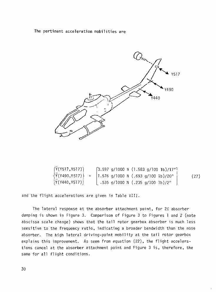
The pertinent acceleration mobilities are

1 Y(Y517,Y517)

Y(Y49O,Y517)

Y(Y44O,Y517)

3.597 g/l000 N (1.583 g/100 I lb)/l7'

1.576 g/l000 N (.693 g/100 lb)/20"

I

(27)

.535 g/1000 N (.235 g/100 lb)/2" _

and‘the flight accelerations are given in Table VIII.

The lateral response at the absorber attachment point, for 2% absorber

damping is shown in Figure 3. Comparison of Figure 3 to Figures 1 and 2 (note

abscissa scale change) shows that the tail rotor gearbox absorber is much less

sensitive to the frequency ratio, indicating a broader bandwidth than the nose

absorber. The high lateral driving-point mobility at the tail rotor gearbox

explains this improvement. As seen from equation (22), the flight accelera-

tions cancel at the absorber attachment point and Figure 3 is, therefore, the

same for all flight conditions.

30

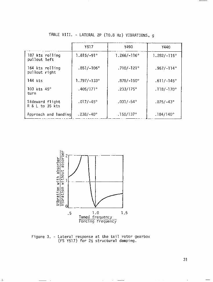
TABLE VIII. - LATERAL 2P (10.8 Hz) VIBRATIONS, g

--___ 187 kts rolling pullout left

164 kts rolling pullout right

144 kts

103 kts 45" turn

Sideward flight R & L to 35 kts

Approach and landin: -- -_ . __-

Y517

1.815/-91"

.851/-106"

1.797/-133"

.405/171"

.017/-45O

.238/-40° - .--

Y490

1.266/-116"

.710/-121"

.878/-150"

.233/175"

.031/-54"

.150/137"

.5 1.0 1.5 Tuned frequency Forcing frequency

Figure 3. - Lateral response at the. tail rotor gearbox (FS Y517) for 2% structural damping.

Y440

1.282/-115"

.967/-114"

.611/-145"

.118/-170"

.075/-43O

.184/140"

31

Comparing Figure 4 with Figures 1 and 2 shows that the tail rotor absorber

effects on fin lateral vibration are much less sensitive to tuning and absorber

damping than the nose absorber effects on vertical vibration at the gunner's

station and stabilizer station. Although the variations in minimum vibration

with damping are small in Figure 4, the minimum is lowest with zero damping,

except in the 187-knot rolling pullout where 5% structural damping gives the

lowest vibration. The absorber tuning frequency for the minimum vibration

varies somewhat with flight condition but is near 90% of 2P in most cases. In

this example a tuning frequency of about 9.7 Hz appears to be the best compro-

mise. Such a selection, as seen from Figure 4, would result in much higher fin

vibration in approach and landing. Referring to Figure 3, a tuning frequency

of about 9.7 Hz gives almost the same vibration at the absorber attachment

point. Figure 5 shows the vibration at FS Y440 for variation in tuning of the

absorber with 2% absorber structural damping. The 9.7 Hz tuning frequency would

have a minor effect at this location in most flight conditions.

The engineer must be cautious of the effects of RPM changes and as a first

approximation the engineer, assuming the vibrations to remain constant with RPM

change given no RPM sweep flight data, would utilize the mobility spectrum data

to create plots similar to those of Figure 4 with an inverted abscissa param-

eter: i.e., variation in forcing frequency for the tuning frequency selected.

This would be done on the interactive computer for all locations and directions

of importance over the RPM range allowable in flight.

32

F

2%

(a) 187 knots rolling pullout left.

1.266 Y'S

2 IL-

d-P- 0%,2%

\I 5x 11

l- I

I- Tc) 144 knots straight

and level.

2

1

G .5 1.0 1.5

.031 g's

.s 1.0 1.5

Tuned frequency/forcing frequency (e) Sideward flight to (f) Approach and landing.

.878 g's

(b) 164 knots rolling pullout right.

.233 g's

(d) 103 knots 45" turn.

35 knots

igure 4. - Effect on fin lateral (FS Y490) of 13.61 kg (30 lb absorber at tail rotor for O%, 2%, and 5% absorber damping.

) lateral structural

33

i!

0. (a ) 187 knots rolling

pullout left.

0 (c) 144 knots straight

and level.

.5 1.0 1.5

.967 g’s

(b) 164 knss rolling pullout right.

.611 _ .118 g's r g's

(d) 103 knots 45" turn.

.075 g's

1

.5 1.0 1 .!

.184 g's

5

Tuned frequency/forcing frequency

(e) Sideward flight to (f) Approach and landing. 35 knots.

Figure 5. - Effect on boom lateral (FS Y440) of 13.61 kg (30 lb) lateral absorber at tail rotor for 2% absorber structural damping.

34

Active Vibration Suppression

Vibration suppression and vibration isolation are distinguished by con-

sidering suppression to imply something other than separating (isolating) the

externally excited structure. Active vibration suppression devices may be

applied without consideration of the physical locations of the external exciting

forces and moments. In this report the term active is used in the customary

sense to indicate a powered device which creates an external force with magni-

tude and phase controlled by reference to a feedback signal of vibration or

strain. The vibration or strain to be controlled will generally not be at the

location of the active vibration suppressor.

Active vibration suppression with time-domain control has been highly

effective in some applications at frequencies far below the lowest blade passage

frequency in helicopters and continuing work in this specialized area may even-

tually be important at helicopter frequencies, but such matters are beyond the

scope of this report. Frequency-domain control of active vibration suppressors,

perhaps by minicomputers, is not as frequency limited as time-domain control

and is close to the state-of-the-art of shaking hardware. For these reasons,

frequency-domain control is implied in the considerations in this report. It

is to be understood in the discussions following that any active vibration

suppressor can, by the methods described for a given frequency, be simultan-

eously applied to other frequencies which are not necessarily limited to har-

monics of main rotor blade passage frequency.

Minimizing the norm of a set of flight accelerations or strains. - Active

vibration suppressors, R in number, can be used to minimize the sum of the

squares of K, greater than R, accelerations or strains. Let the fr complex

vector be that of the forces or moments applied by the R active vibration sup-

pressors and the primed quantities be the resulting complex accelerations and

strains. The matrix equation which defines this situation is

(28)

Kxl Kxl KxR Rx1

35

or, more concisely,

(9k) = {qk} + [ykr] {fr}

Kxl Kxl KxR Rx1

The sum of the squares (Euclidian norm) becomes

(29)

(30)

where * denotes the complex conjugate.

The left hand side of equation (30) is, of course, a real scalar and the

minimum sum of the squares is obtained by setting the partial derivative of this

complex scalar function with respect to the complex transpose of the f, vector

to zero.

= 0 = 2 pkr]*T{qb} ’ 2 [Ykr]*TIIYkr]{fr}‘m’ (31)

The complex forces from the R active vibration suppressors necessary to mini-

mize the sum of the squares (the Euclidian norm or sum of the squares of the

absolute values) of the K (greater than R) vibrations or strains in any flight

condition are

or

(32)

(33)

This process is, except for the minus sign, identical to that of Force Deter-

mination. 5

36

If R were equal to K, then all K accelerations and strains would be zero.

In this case it is necessary to examine the vibration or strain of each impor-

tant motion coordinate which is not of the set of K = R because some of those

of the nonnulled set could have been made much worse. When K is greater than

R, it is necessary to check every significant motion coordinate, including

those of the minimized set, because a reduction in the sum of the squares of

the minimized set does not guarantee that some motion coordinates in the mini-

mized set are not amplified beyond tolerable values. The changed vibration is

determined from

q3 = qj + L’jrl fr lrn) { 1 1x1 1x1 1xR Rx1 (34)

Some Types of Active Vibration Suppressors

The following types of active vibration suppressors are discussed to illus-

trate the application of analytical testing to active vibration suppression.

The list is not intended to be all inelusive and only a cursory examination of

the practicality of the devices is presented.

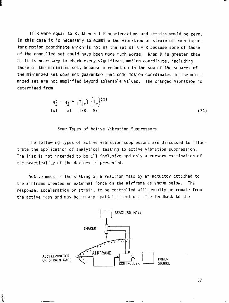
Active mass. - The shaking of a reaction mass by an actuator attached to

the airframe creates an external force on the airframe as shown below. The

response, acceleration or strain, to be controlled will usually be remote from

the active mass and may be in any spatial direction. The feedback to the

REACTION l44SS

ACCELEROMETER OR STRAIN GAGE

CONTROLLER - POkrER SOURCE

37

controller from the shaker may be both force magnitude and phase. To obtain the desired force level on the airframe with minimum reaction mass weight

requires the reaction mass to move through a large displacement.

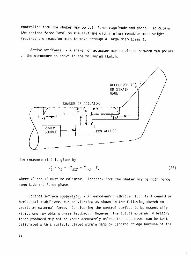
Active stiffness. - A shaker or actuator may be placed between two points

on the structure as shown in the following sketch.

SHAKER OR ACTUATOR

CONTROLLER

The response at j is given by

qj = 9j t(Y. -Y 5x2 jxl) fx (35)

where xl and x2 must be colinear. Feedback from the shaker may be both force

magnitude and force phase.

Control surface suppressor. - An aerodynamic surface, such as a canard or

horizontal stabilizer, can be vibrated as shown in the following sketch to

create an external force. Considering the control surface to be essentially

rigid, one may obtain phase feedback. However, the actual external vibratory

force produced may not be known accurately unless the suppressor can be test

calibrated with a suitably placed strain gage or bending bridge because of the

38

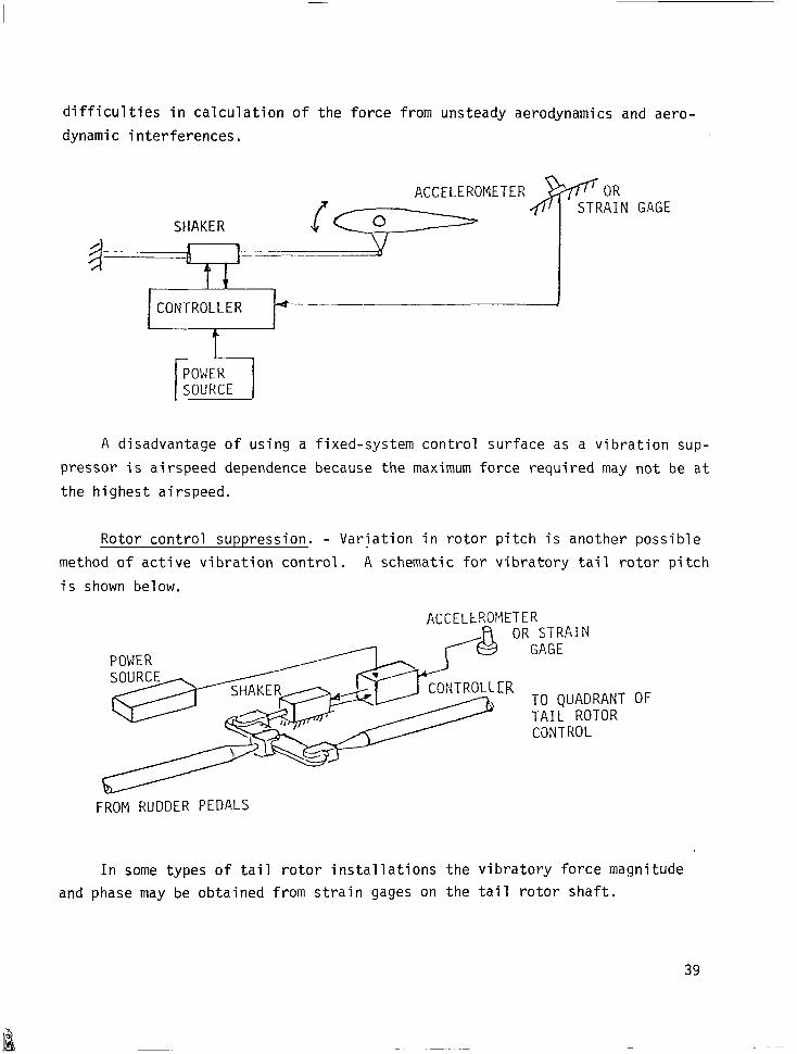
difficulties in calculation of the force from unsteady aerodynamics and aero-

dynamic interferences.

ACCELEROMETER STRAIN GAGE

SHAKER O--QB

-__-

fl

CONTROLLER *------- .t

t

A disadvantage of using a fixed-system control surface as a vibration sup-

pressor is airspeed dependence because the maximum force required may not be at

the highest airspeed.

Rotor control suppression. - Variation in rotor pitch is another possible

method of active vibration control. A schematic for vibratory tail rotor pitch

is shown below.

ACCELEROMETER OR STRAIN

GAGE

XOLLER TO QUADRANT OF

/ ;;;;R;;TOR

FROM RUDDER PEDALS

In some types of tail rotor installations the vibratory force magnitude

and phase may be obtained from strain gages on the tail rotor shaft.

39

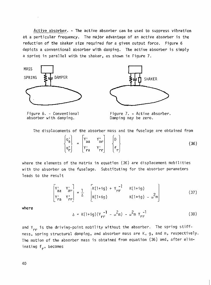
Active absorber. - The active absorber can be used to suppress vibration

at a particular frequency. The major advantage of an active absorber is the

reduction of the shaker size required for a given output force. Figure 6

depicts a conventional absorber with damping. The active absorber is simply

a spring in parallel with the shaker, as shown in Figure 7.

Figure 6. - Conventional Figure 7. - Active absorber. absorber with damping. Damping may be zero.

The displacements of the absorber mass and the fuselage are obtained from

(36)

where the elements of the matrix in equation (36) are displacement mobilities

with the absorber on the fuselage. Substituting for the absorber parameters

leads to the result

” !Ar 1 aa i I K(l+ig) + Y,,' K(l+ig) =-

Y' YLr A (37)

ra i K(l+ig) K(l+ig) - w2m

I

where

A = K(l+ig)(Y,i' - ti2m) - ti2m Yr;' (38)

and Yrr is the driving-point mobility without the absorber. The spring stiff-

ness, spring structural damping, and absorber mass are K, g, and m, respectively.

The motion of the absorber mass is obtained from equation (36) and, after elim-

inating fr, becomes

40

Y’ 9; q; = +

rr

For a shaker force f on the absorber mass and -f on the fuse

determines the displacement of the absorber mass as

lage, equat ion (28)

Y'

9:' Y = $ cl; + (Yia - Yh,) f

and the displacement of the fuselage as

cl;’ = q; - i Y& - Y.&

I f

then Y' q;’ - q;’ = $I - i 1 1 s;+

rr i Y' aa +Ykr-2Yir f

1

(39)

(40)

(41)

(42)

Substituting for the driving-point displacement mobility of the absorber, equa-

tion (22) leads to the result

s; = 9, [K(l+ig) - ti2m] .-

[K(l+ig) - w2m - Y rr K(l+ig) m2m] (43)

where q, is the motion of the fuselage without the absorber.

Equation (42) can then be written as

44' - si' =

w2mqr + (1 - w2m Y,,) f

K(l+ig) (1 - m2m Y,,) 2 -mm

The force on the fuselage is

(44)

fr = K(l+ig) (qg' - qi') - f (45)

41

-

or urn fr =

2 [f + q,K(l + id]

K(l + ig)(l - Yrrw2m) * -urn

and in terms of acceleration 2 w

- ;i,m(l + ig) + 2 f

fr = "T

1 -p t m

"T I i;,! - gii,;

1 L + im Yr; + gj;,; 1 + ig

where aT is the antiresonant frequency at r created by the absorber.

To minimize the denominator with tuning, let

2 w -=m

"T 2 I

;iR rr - gYrL

1 t 1

(46)

(47)

(48)

which sets the real part of the denominator of equation (47) to zero. The

tuning of the active absorber is independent of flight vibrations at the attach-

ment point and the response point whereas the tuning of a conventional absorber

is not. With the tuning condition of equation (48), equation (47) becomes

fr = i q,m (1 t ig) - f w2/QT2

m 'r: I

. . + gv,;

1 + g

From equation (48) the tuning frequency of the active absorber is

I:‘=/c-@q In operation, the minicomputer controller determines the magnitude and phase

required of the shaker from

(49)

(50)

f = $ jf,( W

i i

m[;i,L + q;i I _ ,,I t g), [m, + 90”) + I$,[ m[l + s2]/mr + tan-’ 9

I

(51)

42

The force on the fuse lage at r, fr, for zero vibrat ion at j is determined from

fr = - 'ij

Yjr

(52)

There are two feedback,signals to the controller of the active absorber: the

acceleration at the attachment point and the vibration (strain or acceleration)

of the motion coordinate to be nulled.

Examples of Active Vibration Suppression

The applicability of analytical testing for examining the effects of

active vibration suppressors on airframe vibration is illustrated using AH-1G

ground and flight test vibration data. Equations (33) and (34) are used to

determine the required control forces and the changed vibrations.

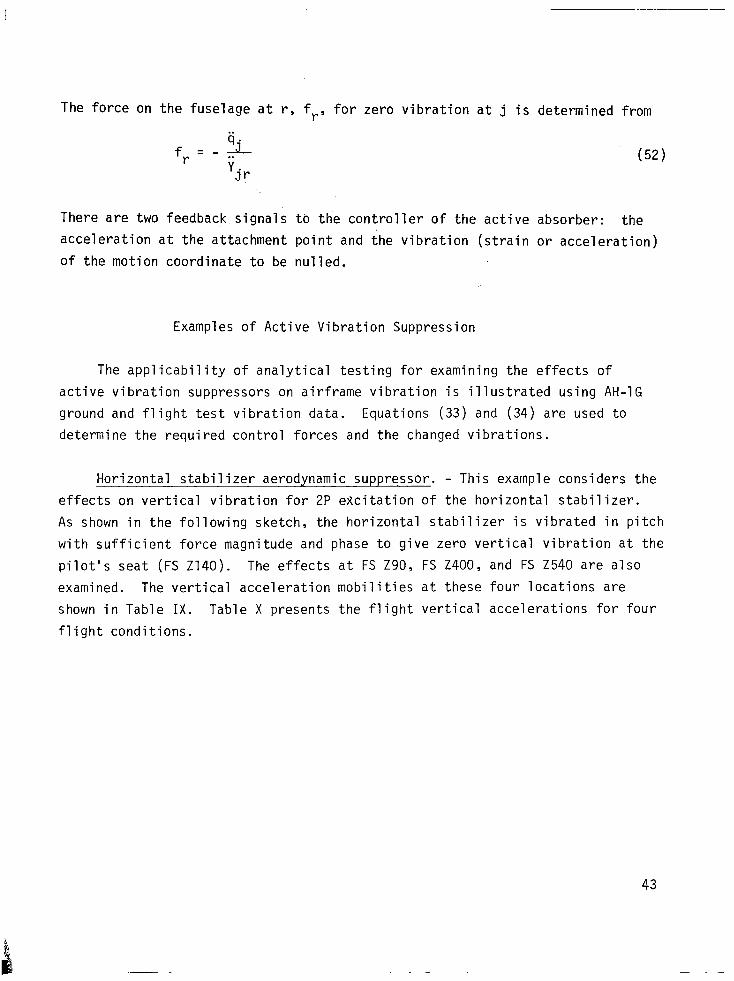
Horizontal stabilizer aerodynamic suppressor. - This example considers the

effects on vertical vibration for 2P excitation of the horizontal stabilizer.

As shown in the following sketch, the horizontal stabilizer is vibrated in pitch

with sufficient force magnitude and phase to give zero vertical vibration at the

pilot's seat (FS 2140). The effects at FS Z90, FS 2400, and FS 2540 are also

examined. The vertical acceleration mobilities at these four locations are

shown in Table IX. Table X presents the flight vertical accelerations for four

flight conditions.

43

At 187 knots, the required force is

fr = - ~ $z140) = _ .147g's/124"

Y(z400,z140) (.065g's/lOOO N)/-84"

- 2261 N(-510 lb)/208'

and similarly for other flight conditions. The vibration at any point is

obtained from equation (34) as

'ij = 'i, + tjr fr

and the results are shown in Table XI.

44

(53)

(54)

TABLE IX. - ACCELERATION MOBILITIES AT 10.8 HZ, g/1000 N (g/l00 lb)

z90

2140

2400

2540

z90

2140

2400

2540 --~___

z90

.103/10" (.046)

.070/6" (.031)

.038/-138" (.017)

.288/g" (.128)

2140

.070/6" (.031)

.052/5O (.023)

.065/-84" (.029)

.124/25" (.055)

.038/-138" (.017)

.065/-84O (.029)

.072/64' (.320)

.672/-32" (.299)

TABLE X. - FLIGHT ACCELERATIONS AT 10.8 HZ, g

187 Knots 164 Knots rolling rolling pullout pullout left right

_---_- .335/120"

.147/124"

.938/68'

1.992/-118"

.322/134" .118/120" .064/124"

.274/114" .114/99O .078/95O

.818/61" .344/44O .237/92"

1.454/-131" .769/-131" .684/-167"

2540

.288/9O (.128)

.124/25O (.055)

.672/-32O (.299)

2.855/-8O :1.270)

144 Knots straight and level

103 Knots 45" turn

Assume that the horizontal stabilizer is vibrated in pitch with sufficient force

magnitude and phase to give zero vertical vibration at the pilot's seat, as

shown by the previous sketch.

45

TABLE XI. VERTICAL VIBRATION AT 10.8 HZ WITH AND WITHOUT , HORIZONTAL STABILIZER AERODYNAMIC SUPPRESSOR, g

187 Knots 164 Knots rolling rolling pullout pullout left right

-2255 N/208" -4204 N/198" (-507 lb) (-945 lb)

With Without With Without

.287 .335 .316 .322

0 . 147 0 .274

2.51 .938 3.798 .818

1.95 1.992 2.523 1.454

144 Knots straight and level

-r

-1748 N/183" (-393 lb)

With Without

.120 .118 ;074 .064

0 .114 0 .078

1.58 .344 1.074 .237

1.263 .769 .592 .684

103 Knots 45" turn

-1197 N/179' (-269 lb)

With Without

The pilot's seat vibration is zero in all flight conditions with a large

increase in vertical vibration at the horizontal stabilizer station on the boom.

The forces required are very large, however.

For purposes of illustration let it be assumed that the horizontal sta-

bilizer has an area of approximately 1 square meter and that trim requirements

would permit a 2P pitch vibration of t 3" maximum producing a vertical force of -

1112 N (250 lb) at 187 knots airspeed. With the maximum force proportional to

the square of the airspeed, the vibrations obtainable with this arrangement are

given in Table XII.

Even with the very large forces of Table XI, zero vibration at the pilot's

seat from an active vibration suppressor at the horizontal stabilizer station

is obtained at the expense of large increases in tail boom vibration with neg-

ligible changes in gunner's seat vibration. The reduction in vibration at

the pilot's seat and gunner's seat using the horizontal stabilizer as an aero-

dynamic suppressor, as shown in Table XII, are not impressive.

46

TABLE XII. - HORIZONTAL STABILIZER FORCED AT 10.8 HZ TO MINIMIZE PILOT’S SEAT VIBRATION

187 knots rolling pullout left

164 knots rolling pullout right

Force at -1112 N/208" -854 N/198" FS 2400 i (-250 lb) (-192 lb)

144 knots straight and level

103 knots 45" turn

-658 N/183" -338 N/179O (-148 lb) (-76 lb)

1 Vertical vibration with and without suppression, g

----pGz z90 .309 .335 .315 .322

2140 .075 .147 .218 .274

2400 1.700 .938 1.409 .818

2540 1.821 1.992 1.298 1.454 I

With Without With Without With Without

.114 .118 .064 .064

.071 .114 .056 .078

.802 .344 .465 .237

.804 .769 .551 .684 I

T-tail aerodynamic suppressor. - The effects on vertical vibration for 2P

excitation of the T-tail, as shown below, are illustrated in this example.

2540

The principal objective is to give zero vertical vibration at the gunner's seat

(FS Z90). The airframe locations and flight conditions are identical to the

previous example. The T-tail horizontal control surface is not required for

47

.----.

trim and can be operated at higher 2P vibratory angles of incidence than the

horizontal stabilizer (FS 2400). Therefore, assuming a T-tail area of approxi-

mately 0.4 square meter , a vibratory force of about 1200 N (270 lb) at 164 knots

can be generated.

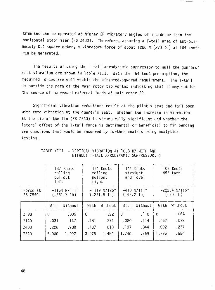
The results of using the T-tail aerodynamic suppressor to null the gunners'

seat vibration are shown in Table XIII. With the 164 knot presumption, the

required forces are well within the airspeed-squared requirement. The T-tail is outside the path of the main rotor tip vortex indicating that it may not be

the source of increased external loads at main rotor 2P.

Significant vibration reductions result at the pilot's seat and tail boom

with zero vibration at the gunner's seat. Whether the increase in vibration

at the tip of the fin (FS 2540) is structurally significant and whether the

lateral offset of the T-tail force is detrimental or beneficial to fin bending

are questions that would be answered by further analsis using analytical

testing.

TABLE XIII. - VERTICAL VIBRATION AT 10.8 HZ WITH AND WITHOUT T-TAIL AERODYNAMIC SUPPRESSOR, g

187 Knots 164 Knots 144 Knots 103 Knots rolling rolling straight 45" turn pullout pullout and level left right

Force at -1164 N/111" -1119 N/125" -410 N/ll1° -222.4 N/115" FS 2540 (-261.7 lb) (-251.6 lb) (-92.2 lb) (-50 lb)

With Without With Without With Without With Without

z 90 0 .335 0 .322 0 .118 0 .064

2140 .031 .147 .181 .274 .080 .114 .062 .078

2400 .226 .938 .437 .818 .197 .344 .092 .237

2540 5.000 1.992 3.975 1.454 1.740 .769 1.295 .684 2 L

48

-

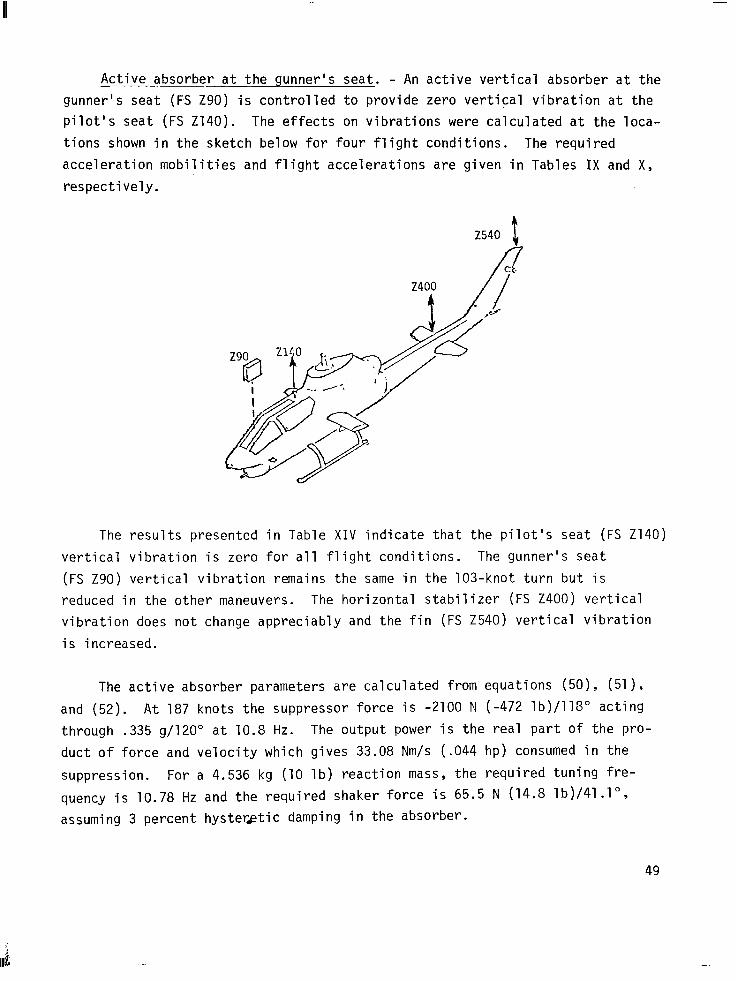
Active absorber at the gunner's seat. - An active vertical absorber at the

gunner's seat (FS Z90) is controlled to provide zero vertical vibration at the

pilot's seat (FS 2140). The effects on vibrations were calculated at the loca-

tions shown in the sketch below for four flight conditions. The required

acceleration mobilities and flight accelerations are given in Tables IX and X,

respectively.

2540 s

The results presented in Table XIV indicate that the pilot's seat (FS 2140)

vertical vibration is zero for all flight conditions. The gunner's seat

(FS Z90) vertical vibration remains the same in the 103-knot turn but is

reduced in the other maneuvers. The horizontal stabilizer (FS 2400) vertical

vibration does not change appreciably and the fin (FS 2540) vertical vibration

is increased.

The active absorber parameters are calculated from equations (50), (51),

and (52). At 187 knots the suppressor force is -2100 N (-472 lb)/llSO acting

through .335 g/120" at 10.8 Hz. The output power is the real part of the pro-

duct of force and velocity which gives 33.08 Nm/s (.044 hp) consumed in the

suppression. For a 4.536 kg (10 lb) reaction mass, the required tuning fre-

quency is 10.78 Hz and the required shaker force is 65.5 N (14.8 lb)/41.1",

assuming 3 percent hysterptic damping in the absorber.

49

TABLE XIV. - VERTICAL VIBRATION AT 10.8 HZ WITH AND WITHOUT ACTIVE ABSORBER AT GUNNER'S STATION, g

187 Knots rolling pullout left

-2108 N/ll8O (-474 lb)

With Without

.723 .335

.ooo .747

.939 .938

2.315 1.992

------ - ~.___. 764 Knots 744 Knots 103 Knots rolling straight 45" turn pu7 lout and level right

~--p-b- ~-

---- -__ ____ -3732 N/108" -1637

(-839 7b) N/93-' -7721 N/89"

(-368 7b) (-252 lb)

With Without With Without With Without

.732 .322 .066 .178 .064 .064

. 000 .274 . 000 .174 000 .078 .

.834 .818 .349 .344 .272 .237

2.751 1.454 1.117 .769 .787 .684

Active absorber at the tail rotor. - In this example the objective is to

produce zero lateral vibration on the fin (FS Y490) at 10.8 Hz. An active

'lateral absorber at the tail rotor gearbox was selected as the vibration sup-

pressor, although excitation of tail rotor pitch is an alternative. The pre-

ference of harmonic control of the tail rotor or an active absorber depends on

many factors among which are tail rotor blade loads. Main rotor 2P excitation

of the tail rotor may increase or decrease tail rotor fatigue life and this

requires additional investigation. The effects on lateral flight accelerations

were calculated at the locations shown in the following sketch for four flight

conditions. The required acceleration mobilities and flight accelerations are

shown in Tables XV and XVI, respectively. The flight conditions are identical

to the previous example.

The results shown in Table XVII indicate that the tail rotor gearbox vibra-

tion is negligibly affected in the rolling pullouts, but significantly reduced

in 144-knot level flight and in the 103-knot turn. The vibration at FS Y440 is

reduced substantially in the 187-knot left rolling pullout and at 744-knot level

flight, reduced somewhat in the 164-knot right rolling pullout, and increased in

the 103-knot turn. Changes in pilot and gunner vibration are not significant.

As expected, the fin (FS Y490) vibration is zero for all flight conditions. A d

50

TABLE XV. - ACCELERATION MOBILITIES AT 70.8 HZ RELATIVE TO FS Y517 (TAIL ROTOR LATERAL), g/l000 N (g/l00 lb)

I __----- I

TABLE XVI. - LATERAL FLIGHT VIBRATION, g .--~--- .___-~_-.__ .--F_-- ___-

1 Fuselage stations Y577 ---T-- Y490 - -- Y440 I Yl40

1 J

7.815/-97" 1.266/-116" 1.282/-115" .123/-96'

.857/-106" .710/-121" .967/-114" .118/-89"

1.637/-138" .878/-150" .611/-145" .055/-114"

.405/171" .233/175" .048/-95" .048/-95"

51

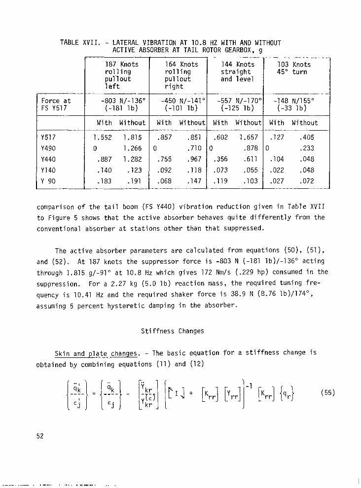
TABLE XVII. - LATERAL VIBRATION AT 10.8 HZ WITH AND WITHOUT ACTIVE ABSORBER AT TAIL ROTOR GEARBOX, g

Force at FS Y517

Y577

Y490

Y440

Y740

Y 90

187 Knots 764 Knots rol.ling rolling pullout pullout left right

-803 N/-136" -450 N/-141' (-181 lb) (-101 lb)

With Without With Without

7.552 7.875 .857 .857

0 1.266 0 .710

.887 1.282 .755 .967

.140 .723 .092 .718

.183 .191 .068 .747

744 Knots straight and level

-557 N/-170' -148 N/155" (-125 lb) (-33 lb)

With Without With Without

.602 7.657 .727 .405

0 .878 0 .233

.356 .611 .104 .048

.073 .055 -022 .048

.119 .103 .027 .072

- _. ----_ .._ 103 Knots 45" turn

comparison of the tail boom (FS Y440) vibration reduction given in Table XVII

to Figure 5 shows that the active absorber behaves quite differently from the

conventional absorber at stations other than that suppressed.

The active absorber parameters are calculated from equations (50), (57),

and (52). At 187 knots the suppressor force is -803 N (-181 lb)/-736" acting

through 1.815 g/-91" at 10.8 Hz which gives 172 Nm/s (.229 hp) consumed in the

suppression. For a 2.27 kg (5.0 lb) reaction mass, the required tuning fre-

quency is 10.41 Hz and the required shaker force is 38.9 N (8.76 lb)/l74",

assuming 5 percent hysteretic damping in the absorber.

Stiffness Changes

Skin and plate changes. - The basic equation for a stiffness change is

obtained by combining equations (11) and (12)

52

- . . . . . . . . . 1.11 . . . . ..I... ,, I

where Krr II 1 is the stiffness matrix of the skin section as a free body,

the vector of flight displacements at the change coordinates and Yrr

c I matrix of displacement mobilities of the airframe at the change coordinates. A

to a plate, has negligible transverse stiffness and the coor-

are on the surface of the airframe. The differences among the

are most a stiffness change. It would be impractical in most cases to from flight accelerometers alone

because of the small difference between large numbers. This problem, however,

is resolved using strain gages.

Figure 8 shows a skin section and the rectangular coordinates of the rele-

vant stiffness matrix. The skin may be of nonhomogeneous materials with noncon-

stant thickness, such as a two dimensionally tapered composite, with directional

modulii of elasticity or a simple metal sheet. Only the stiffness matrix needs

to be known in applying equation (55). The effects of proportional or nonpro-

portional damping may be included in equation (55) by replacing Krr with a [ I

complex matrix which is the sum of the real stiffness matrix and an imaginary

damping matrix, frequency dependent for viscous damping and frequency indepen-

dent for hysteretic damping.

It is immaterial to the analytical testing approach whether the surface of

the helicopter at which the skin or plate change is to be made is flat or

curved.

For n nodes on a sk'in there are 2n rectangular coordinates and the stiff-

ness matrix (the matrix of the partial derivatives of force to displacement) is

a square matrix of order 2n and rank 2n - 3. For practical flight and shake

test measurements the skin section may be modeled in terms of 2n - 3 strain

coordinates as shown in Figure 9.

The displacement mobility matrix for the strain coordinates of, for example,

the skin section of Figure 9 may be determined as shown in Figure 10 where equal

and opposite forces are applied across a distance 6. This type of displacement

mobility (influence coefficient) matrix becomes

53

Figure 8. - Rectangular coordinates of a skin section with nine nodes.

Figure 9. - Strain coordinates of a skin section with nine nodes.

54

-

-----

f. J+7

Figure 70. - The jkth element of the strain stiffness matrix is a(fj+l - fj-l)

a(qk+l - qk-1 1'

[ 1 ,k) = aAqk aaf.

J (56)

which is, of course, nonsingular and may be inverted to give a stiffness matrix

(57)

where

Af. = J i Cfj+l - fj-7 1

and

Aqk = qkt' - qk-'

If, on the other hand, the conventional type 2n x 2n stiffness matrix K

is available the strain type stiffness matrix k may be found using a coordinate

transformation. Note that

(58)

55

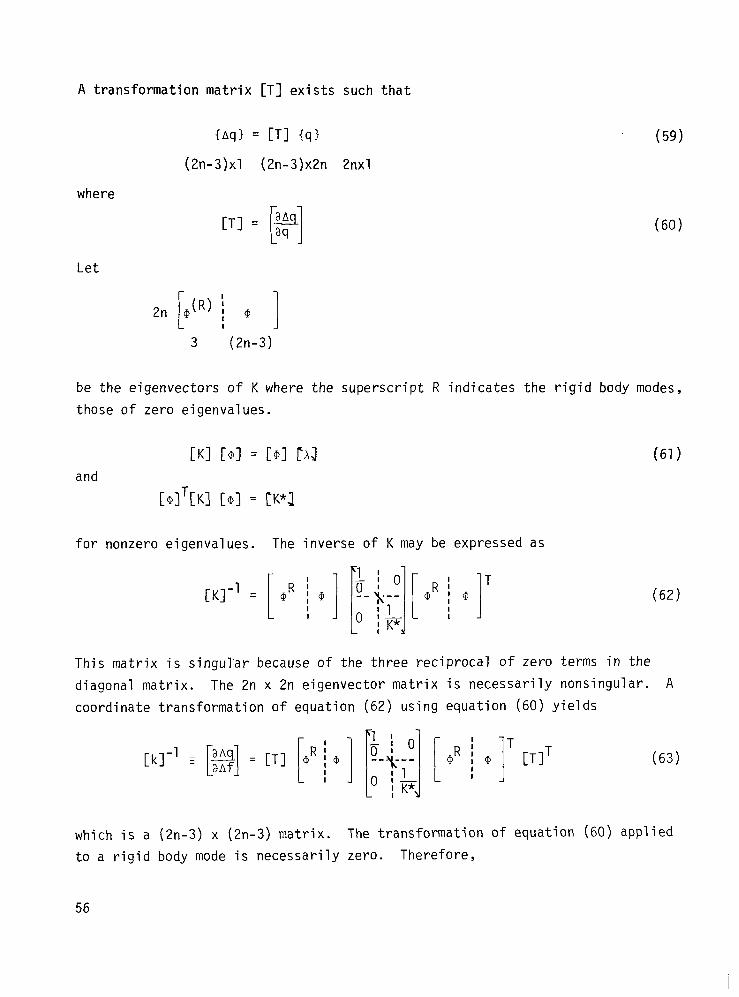
A transformation matrix [T] exists such that

(Aq) = CT] (ql

(2n-3)x1 (2n-3)x2n 2nxl

where

[T] = F [ I

Let

(59)

(60)

2n [ 0(R) i @

I I 3 (2n-3)

be the eigenvectors of K where the superscript R indicates the rigid body modes,

those of zero eigenvalues.

and

CKI [@I = [@I Cd (67 >

for nonzero eigenvalues. The inverse of K may be expressed as

I i cp ' I

T (62)

I

This matrix is singul.ar because of the three ret iprocal of zero terms in the

diagonal matrix. The 2n x 2n eigenvector matrix is necessarily nonsingular. A

coordinate transformation of equation (62) using equation (60) yields

(63)

which is a (2n-3) x (2n-3) matrix. The transformation of equation (60) app7ied

to a rigid body mode is necessarily zero. Therefore,

56

(64)

The 0 x O/O indeterminant terms in the product are zero and equation (64) may

be written as

[TIE@] [$-I bITITIT

from which it follows that k, a nonsingular matrix of order (2n-3), is given by

[s] = [k] = ([T][B]]-~ rK*J ([Tl[ml]-'

-T ~olT~KI[ol (65)

It is also necessary to establish the types of mobility measurements which

are practical in an actual airframe.

For forces fj+, and fjSl only in-figure 9,

Aqk = aqk-l f aqk 1 - ___

j-l afjtl jtl - xI- f

j-l (66) j-7

But, -fjSl = fjtl = Afj. Therefore

Aqk aqk+' af aqk+l af aqk-l aqk-l af.=af---

- -

J jtl j-l jtl + af j-l

= 'ktl,i 'j+l,i - 'ktl,i 'j-l,i - 'k-7,i 'j+l,i

' 'k-1,i 'j-1,i Fi I =

'k+l,i - 'k-1,i 1 I 'j+l,i - 'j-1,i 1 Fi (67)

57

For forces only at j

or, for any number of forces,

Similarly,

i

With a strain stiffness matrix, equation (55) becomes

(69)

(70)

In the case of a plate, there is transverse stiffness and nonnegligible

mass. The aircraft is tested with n accelerometers perpendicular to the sur-

face, for n attachment points, in addition to the strain gages, as shown in

Figure 77.

Numerical example of a transformation to a strain stiffness. - The six

pinned rods of Figure 12 provide a simple illustration of the transformation

from a stiffness matrix with rectangular coordinates to one with strain coordi-

nates.

In the stiffness matrix with rectangular coordinates, shown following

Figures 11 and 12, the k terms are axial spring rates subscripted with the ter-

minal positions of the rods.

58

/ \

\

\ 20

Figure 11. - A plate change with nine attachment points.

Figure 12. - Simple bar truss with rectangular coordinates.

59

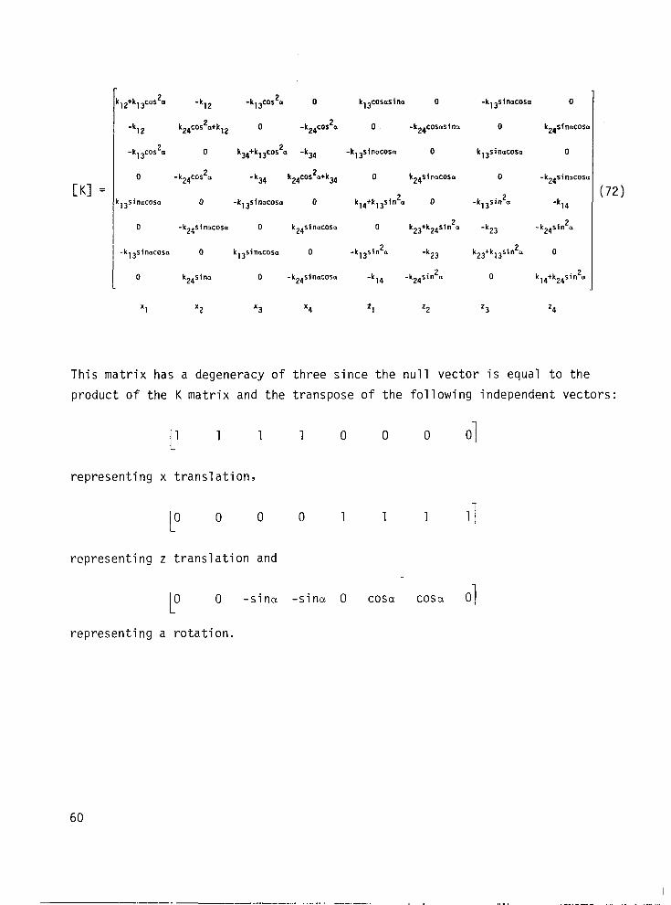
[Kl =

r ,2+k,3cos2m -k12 -k,3cos2m 0 k,3cosdina 0 -k,3sinacosa 0

-k12 k24cos2a+k,2 0 -k24cos2a 0 -k24cosas1"a 0 k24sina~~s

-k,3cos2a 0 k34+k,3cos2a -k34 -k,3sinocosa 0 k13simcosa 0

0 -k24cos2a -k34 k24cos2m+k34 0 k24s1nncos. 0 -k24sinacos

,3S1”UCOS” 0 -k13sinacosa 0 k,4+k,3s1"2a 0 -k,3sin2a -k14

0 -k24s1nacosa 0 k24sinacosa 0 k23+k24sin2a -'23 -k24sin2a

-k,3sinacosn 0 k,3sinacosa 0 -k13sin2a -k23 k23+k,3sin2a 0

0 k24sina 0 -k24s1nacosa -k14 -k24sin 2 D 0 k,4+k24sin 2 (1

9 x2 x3 x4 21 z2 z3 z4

(72)

This matrix has a degeneracy of three since the null vector is equal to the

product of the K matrix and the transpose of the following independent vectors:

1 1 1 11 0

representing x translation,

1 0 0 0 0 1

representing z translation and

1 0 0 -sina -sincr 0

representing a rotation.

60

0

1

cosa

0

1

cosa

01

11

01

-.---.- . ----..- . . ..__ - -_.-.. ._. _. _.._-,--,, , .

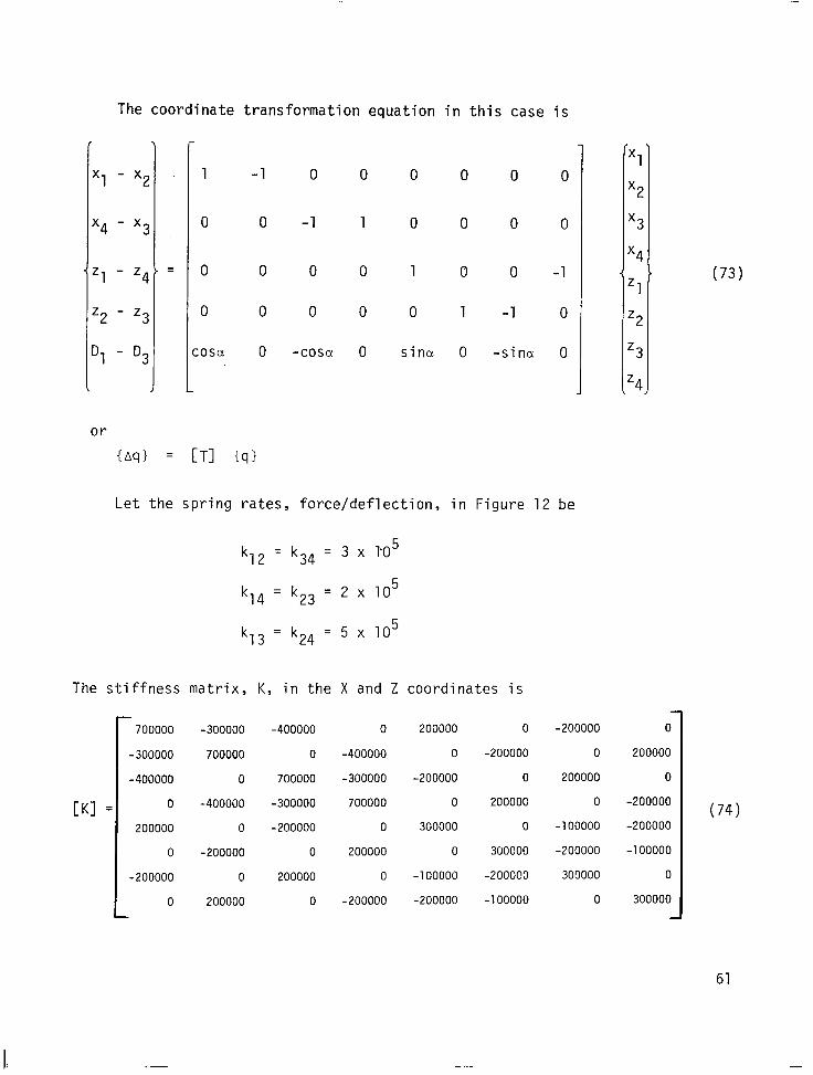
The coordinate transformation equation in this case is

or

{Aql

=

1 -1 0 0 0 0 0 0

0 0 -1 1 0 0 0 0

0 0 0 0 1 0 0 -1

0 0 0 0 0 l-l 0

:osa 0 -cosa 0 sir-w 0 -sina 0

= [Tl Cql

Let the spring rates, force/deflection, in Figure 12 be

k12 = k34 = 3 x l-O5

k14 = k23 = 2 x lo5

k13 = k24 = 5 x lo5

The stiffness matrix, I(, in the X and Z coordinates is

[Kl q

700000 -300000

-300000 700000

-400000 0

0 -400000

200000 0

0 -200000

-200000 0

0 200000

-400000

0

700000

-300000

-200000

0

200000

0

0

-400000

-300000

700000

0

200000

0

-200000

200000

0

-200000

0

300000

0

-100000

-200000

0 -200000

-200000 0

0 200000

200000 0

0 -100000

300000 -200000

-200000 300000

-100000 0

I \ xl

x2

x3

x4 < *

zl

z2

z3

,z4,

0

200000

0

-200000

-200000

-100000

0

300000

1

(73)

(74)

61

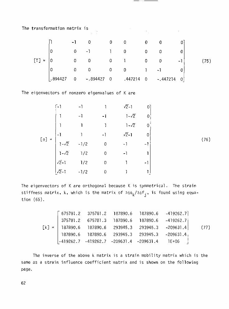
The transformation matrix is

1 -1 0 0 0 0

0 0 -1 10 0

[T] = 0 0 0 0 1 0

0 0 0 0 0 1

.894427 0 -.894427 0 .447214 0

The eigenvectors of nonzero eigenvalues of K are

--1

1

1

-1 [@I =

1-e

1-n

n-1

C-1

-1

-1

1

1

-l/2

l/2

l/2

-l/Z

1

-1

1

-1

0

0

0

0

n-1

l-47

1-n

n-1

-1

-1

1

1

0

0

0

-1

-.4472

0

0

-1 (75)

0

14 0 I

The eigenvectors of K are orthogonal because K is symmetrical. The strain

stiffness matrix, k, which is the matrix of aciqk/aafj, is found using equa-

tion (65).

[kl =

675781.2 375781.2 187890.6 187890.6 -419262.7

375781.2 675781.3 187390.6 187890.6 -419262.7

187890.6 187890.6 293945.3 293945.3 -209631.4

187890.6 187890.6 293945.3 293945.3 -209631.4

-419262.7 -419262.7 -209631.4 -209631.4 lEtO6

(76)

(77)

The inverse of the above k matrix is a strain mobility matrix which is the

same as a strain influence coefficient matrix and is shown on the following

paw.

62

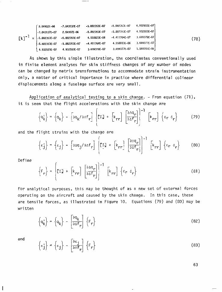
[k]-' =

2.54902E-06 -7.843137E-07 -5.882353E-07 -5.8132353E-07 4.932503E-07

-7.843137E-07 2.54902E-06 -5.882353E-07 -5.882353E-07 4.932503E-07

-5.882353E-07 -5.882353E-07 4.558823E-06 -4.411764E-07 3,699378E-07 (78)

-5.882353E-07 -5.882353E-07 -4.411764E-07 4.558823E-06 3.699377E-07

,4.932503E-07 4.932503E-07 3.699378E-07 3.699377E-07 1.568704E-06

As shown by this simple illustration, the coordinates conventionally used in finite element analyses for skin stiffness changes of any number of nodes

can be changed by matrix transformations to accommodate strain instrumentation

only, a matter of critical importance in practice where differential colinear

displacements along a fuselage surface are very small.

Application of analytical testing to a skin change. - From equation (71),

it is seen that the flight accelerations with the skin change are \ {qi} = {qk} - [aqk/aaf,] [rrd ’ brr] [?I -’ krr] {&r sr} (79) ,

{LJ:) = {‘j> - ~‘q

Define I

{Fr} = lCrl + [k,,] [q] -’ km-1 { +

and the flight strains with the change are I

[i$]]-' [krr] {+ 'i-j (80)

(81)

For analytical purposes, this may be thought of as a new set of external forces

operating on the aircraft and caused by the skin change. In this case, these

are tensile forces, as illustrated in Figure 10. Equations (79) and (80) may be

written

and

(82)

{E.j} = {'j} - [&] {Fr} (83)

63

The strain stiffness matrix, krr, of the contemplated skin change is obtained

from a finite element analysis as discussed above. From flight tests of the

baseline aircraft, the accelerations {qkI and the strains 1~~) at coordinates

of interest are known. From modal shake testing (or finite element analysis)

of the baseline aircraft the orthonormal modes [\11,] and and the fre-

quency function [F] are known.

The nonflying shake test aircraft is instrumented with strain gages as

shown in Figure 13 for a nine node change and a modal analysis test is done to

6) obtain the orthonormal modal elements of yr [ I

. The distance between nodes

should be as large as possible to avoid large orthonormal strain mode elements

at very high frequencies which occur when there is negligible inertial effect

at a node. Long gage strain gages are preferred to minimize local effects.

STRAIN GAGE (gyp.)

Figure 13. - Strain gages on the fuselage for flight and shake tests.

64

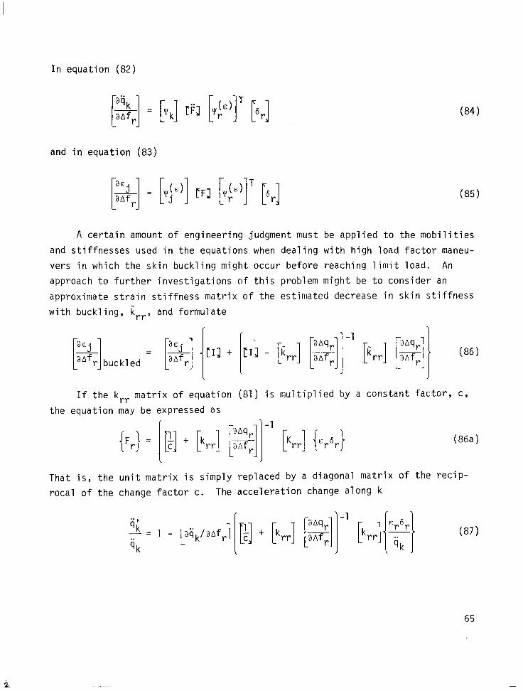
In equation (82)

and in equation (83)

[qj = [$)I CFJ [WbE)]' br] (85)

(84)

A certain amount of engineering judgment must be applied to the mobilities

and stiffnesses used in the equations when dealing with high load factor maneu-

vers in which the skin buckling might occur before reaching limit load. An

approach to further investigations of this problem might be to consider an

approximate strain stiffness matrix of the estimated decrease in skin stiffness

with buckling, krr, and formulate

w,

[I: aaf,

(86)

If the k,, matrix of equation (81) is multiplied by a constant factor, c,

the equation may be expressed as

{Fr} = I[;] + krr] [?]I-' [Krr] tErSr}

That is, the unit matrix is simply replaced by a diagonal matrix of the recip-

rocal of the change factor c. The acceleration change along k

‘i;, - = 1 - ik 1

aqk/aafr 1

(86a)

65

--

and the strain change along j

for any flight condition.

E 6

i I

rr “j”j

(88)

Equation (88) may be displayed as a function of c, the change factor, as

shown in Figure 14. In a skin change, c would be the proportionality of skin

thickness of the change. In this manner, the effects of the contemplated

change at many different fuselage locations in a variety of maneuvers can be

systematically evaluated to select the most suitable compromise of thickness

factor.

Strap, Stringer and Strut Changes. - For a stringer or strap change, as

shown in Figure 15, the stiffness matrix of equation (71) is diagonal with each

element being the axial stiffness of the corresponding section of the strap.

Equation (71) may then be expressed as

In evaluating the effects of a possible strut addition where there is no

strut at present, as in Figure 16, there is no existing surface on which to

place strain gages. A pin-ended tube can be put in the position of the strut

to activate a differential motion transducer such as a linear differential

voltage transducer or potentiometer. The term k,, is the axial stiffness of

the strut in equation (89) which may be written

(90)

66

0 1 2 3 4

CHANGE FACTOR

Figure 14. - The change in flight response of any coordinate in any maneuver displayed as a function of a change factor, such as skin thickness.

-RAIN GAGE (TYP.)

Figure 15. - A strap change of stiffness.

67

Figure 16. - A strut type change and differential transducer instrumentation in shake test.

68

TECHNIQUES AND PROCEDURES FOR VIBRATION TESTING

OF THE AH-1G HELICOPTER

The development of effective techniques for shaking the AH-1G and analy-

zing the acquired vibration data constituted a major part of the research work

associated with analytical testing. The validity of the methods employed rests heavily upon the consistency between the measured structural mobilities and the

theoretical models for which these mobilities are derived. This consistency is

critical since the measured mobilities are used not only for obtaining the

global modal parameters of the test vehicle, but also to derive mobilities

which were not measured directly.

Digital signal analyzers have made it possible to measure the response of

structures to any physically realizable excitation. However, the interpreta-

tion of measured structure to specified excitation forces is subject to the

mathematical model used in the process of analyzing the data. The model may be

more or less sophisticated, depending on the test data. The dynamic testing of

a structure like the helicopter poses a number of specific problems. These

problems are associated with: (1) the size and complexity of structure;

(2) nonuniform distribution of mass, stiffness, and damping; and (3) the cor-

rect application of linear vibration theory to the process of data acquisition

and analysis.

It has been implied that the techniques adopted for the structural dynamic

testing are closely related with the theory underlying the vibration analysis.

A discussion of the specific test procedures must necessarily be preceded by

a brief summary of the theoretical considerations. This chapter addresses:

(1) the theory of the generalized linear structure; (2) the principal charac-

teristics of acceleration mobility data; (3) testing procedures for global

parameters and the estimation of these parameters; (4) testing procedures for

obtaining mode shapes and the method of calculating mode shapes; and

(5) methods for deriving mobilities from modal data.

69

Theory of the Generalized Linear Structure

The dynamic properties of any structure can always be characterized by a

relationship between a selected set of motion coordinates and the set of exter-

nally,applied forces, i.e.:

The character of the structure implied in equation (91) will be termed mobility.

If the motion vector is a vector of displacements/velocities/accelerations, the

character of the structure is termed displacement/velocity/acceleration mobility,

respectively.

The central phenomenon of vibration theory is cycl

the quantities that go into equation (91) are generally

domain; for example, in acceleration measurements:

ic oscillation, hence

sought in the frequency

(92)

where {j;(w)1 is the Fourier transform of the accelerations; [y(,)] is the

acceleration mobility matrix; and {f(w)1 is the Fourier transform of the vector

of generalized forces, compatible with the selected set of coordinates.

From a measurement standpoint, the jkth element of the matrix [V(U)]

relates the acceleration measured along the jth coordinate when the only force

acting on the structure is that applied along the kth coordinate; i.e.:

yj(w) = Yjk(W) fk(U) when f. lfk

=0 (93’)

Linear vibration response of a structure may be characterized by the following

conditions: (1) the response of the structure to random forcing is stationary

in time (i.e., forced vibrations are steady); (2) the elements of the matrix

[V(U)] are functions of frequency only, and depend on neither the motion coordi-

nates, nor the forcing vector; and (3) the mobility matrix [V(O)] is symmetric;

i.e.,'i ='\i jk kj'

70

The foregoing conditions have specific practical implications in vibration

testing and analysis. The first,condition is necessary for any structure to survive continuous operation under arbitrary dynamic excitation. The second condition more or less stipulates the type of shake test data thatis adequate

for analysis based on a linear model of the structure. If the mobility func-

tions measured for different force levels are not the same, the assumption of

linearity is not satisfied. This is usually the case when only part of the

structure may be participating in the response. As the force level is

increased, more and more of the relevant motion coordinates of the structure

start to participate in the response. The range of linear response is reached

only when the measured mobility remains unchanged with changing force levels.

The third requirement is that of reciprocity. If the shaking and measurement

stations are interchanged, the same mobility should be recorded, otherwise the

[Y] matrix will not be symmetric, as required by the linear model.

It is important to note that, in the foregoing characterization of a linear

system, no assumptions are made about the nature of the damping mechanisms

occurring in the structures. All the conditions required for linear modeling

can be verified in the process of the actual shake test of the structure.

The relationship between the Fourier transform of the force vector and

that of the displacement vector of a steadily vibrating undamped multiple

degree of freedom system can be written as:

- w * [Ml + [Kl] fy(w)> = f(o)

where [M] and [K] are real, symmetric mass and stiffness matrices, respectively.

Thus, the displacement mobility matrix for an undamped system is simply:

[Y(,)l, = [- w* [Ml + [Kl]-’ (95)

The presence of damping in its most general form can be modeled by introducing

a frequency dependent complex damping matrix into equation (951, i.e.:

CWI, = (- cd2 [Ml + CK] + [DR(w)] + i[D'(w)]lW1 (96)

71

It is to be carefully noted that this analytical development has meaning

only in the frequency domain for the general case of damping. This is mainly because the physical quantities that can be used to characterize the arbitrary

damping of a structure are related to the energy dissipated per cycle of oscil-

lation. In cases where the time domain, force/motion relationship, repre-

senting the damping mechanism is known, the damped equations of motion can be

developed in the time domain and then Fourier transformed into the frequency

domain. However, taking the inverse Fourier transform of the frequency-domain

equations that may adequately describe an arbitrarily damped system may not

yield a time-domain system of equations that makes physical sense. In other

words, arbitrary damping mechanisms may not be susceptible to a time-domain

description. Mathematical models, developed from time-domain equations of

motion, usually fail to identify global characteristics of structures with sig-

nificant damping.

In general, the elements of [DR(w)] are small, compared to those of the

[K] matrix. Also, in order for reciprocity conditions to be met and for energy

to be dissipated, the damping matrix must be symmetric and non-negative

definite over the entire frequency range.

For a damped system, then:

I [K] + i[D(w)] - w2 [M]] {y(w)> = {f(w)) (97)

Consider the complex, frequency dependent characteristic value problem:

[Kl + i[D(ti)] C$> = x(u)CMIC~I 1

where ($3 = (~~1 t ii@'} is the complex characteristic vector which can be

assumed to be frequency independent; A(~) = hR(w) + ihI is the frequency

dependent complex eigenvalue.

(98)

If combinations of

tion (98), then:

A~(,,,), ($lk 1 exist, which satisfy equa-

72

[D(w)]

W; ([Kl + i[D(w)l {$jk 1 = +$&d; [M]b$~, (100) {@IT denotes the transpose of (41. By virtue of the symmetry of the [K], CM],

lead to the following orthogon- and [D(U)] matrices, equations (99) and (100)

ality relationships:

and

where:

W; [[Kl + i[D(U)]]{$}k = [k j

+ id

6jk

j Cw)

T

(101)

1 6jk (102)

m. J = r~}j [MI E~lj

kj = {~}3 [K] ~~lj

dj(w) = {~~: [D(w)] '~'j

'jk =Oj#k lj=k

(103)

(104)

(105)

(106)

It follows that:

. - .

W; [[Kl - u2 [Ml + i[D(dl W ] k = [k,j - m2mj + idj(U)]Sjk

(107)

73

If the vectors Ce~j exist, it can easily be verified that only the imaginary

parts of Xj(w) need be frequency dependent. So that:

Aj(w) = A! + i 1: (w) (108)

Indeed, by post-multiplying the transpose of equation (98) by 1613, which is the complex conjugate of I$lj, the following equation is obtained:

io}J [WI +ico(dl) I~~3 = ‘j(w) 1~}3 CMI 10}3 (109) -

Similarly, the complex conjugate of equation

to get:

From equations (109) and (110);

and

(98) can be premultiplied by

(112)

The right hand side of equation (111) is a frequency independent quantity. How-

ever, the right hand side of equation (112 ) is frequency dependent, establishing

the validity of the claim made in equation (108).

(111)

A complex L x N modal matrix [o] can be defined such that its jth column

is the L x 1 vector I$Jj; j = I, 2, . . . N, where L is the number of coordinates

chosen to describe the system and N is the number of modes of the.system. In

principle, N is infinite; in practice, over a given frequency range, only a

finite number of system modes are necessary. ‘C

74

Equation (97) can be rewritten to give,

Iy(w)l = [Q] (CK] - w2 [Ml + i[D(w)] J I

[Q] -' C@lTCf(U)l (113)

and, using the orthogonality relationships, leads to the results,

(Y(w)> = Co]

c

1

L (AjR - w2) + iA; mj

I I

[@IT {f(w)>

By definition: {y(w)1 = [Y(w)]Cf(w)l ; hence,

1

(A,R - w2) + i xi(~)

(114)

(“5)

A: and A:(U) have units of (frequency)2 and, from physical considerations , both

A," and X$U) are positive. It is, therefore, possible to define:

(116)

and

(117)

The matrix of modal acceleration coefficients of the nth mode is defined as:

The acceleration mobility matrix and the displacement mobility matrix are

related by:

(118)

[$I)] = - u2 [Y(w)] (‘19)

75

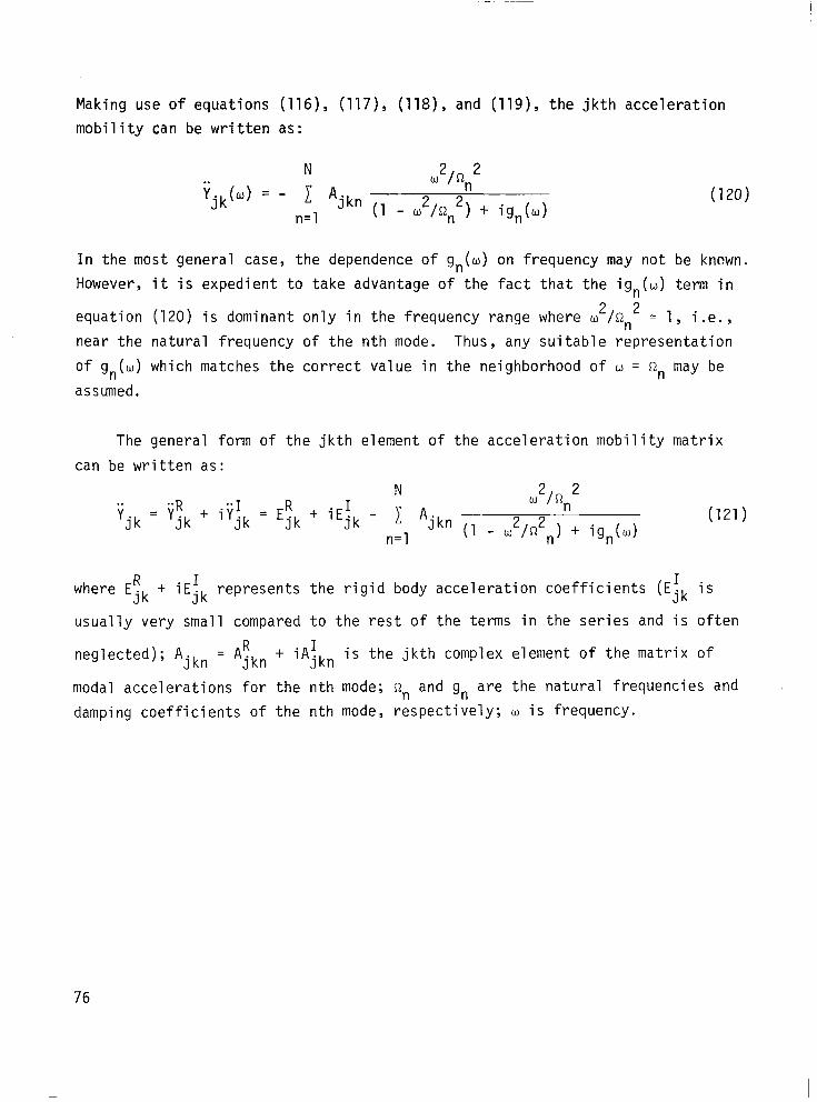
Making use of equations (116), (117), (118), and (119), the jkth acceleration

mobility can be written as:

N

vjk(u) = - 1 Ajkn u2/ctn2

n=l (1 - u2/nn2 1 + igJd (120)

In the most general case, the dependence of g,(w) on frequency may not be known.

However, it is expedient to take advantage of the fact that the ign(w) term in

equation (120) is dominant only in the frequency range where w2/fin2 = 1, i.e.,

near the natural frequency of the nth mode. Thus, any suitable representation

of gn(w) which matches the correct value in the neighborhood of w = R,, may be

assumed.

The general form of the jkth element of the acceleration mobility matrix

can be written as:

N

;i ;iR jk = jk

+ i;iI = ER . I u21Qn2

jk jk ' 1Ejk - c Ajkn ll _ 33

(121)

n=l n) + ig,(w)

where ER jk

+ iEik represents the rigid body acceleration coefficients (Eik is

usually very small compared to the rest of the terms in the series and is often

neglected); Ajkn = Agkn + iA1 jkn is the jkth complex element of the matrix of

modal accelerations for the nth mode; c$, and g, are the natural frequencies and

damping coefficients of the nth mode, respectively; w is frequency.

76

Characteristics of Acceleration Mobility Data

Mode frequency functions .--

The real and imaginary parts of fjk can be written as:

and

or:

N ;iR = ER

jk jk - c [ n=l

AjRkn if (w) - Ajkn 1; (w)]

N i;I EI

jk = jk - n=l

f; (w) + Aikn F; (w)]

N . . Y ER I jk = jk + iEjk - 1 Ajkn 'n (w)

n=l

where the mode frequency functions are defined as:

and

u2hn2 ("2/Qn2 - 1) F; (w) ! ___

(u2/nn2 - 1)2 + g,2

gn u2/n 2

F; (w) : (u2/nn2 - 1,; + gn2

Fn (IA) = FE (w) t iFi (w) (127)

(122)

(123)

(124)

(125)

(126)

Equations (122), (123), and (124) represent the measured acceleration mobility

as a linear combination of the mode functions. It is, therefore, important to

acquire a familiarity with the basic characteristics of the mode functions of

damped systems and the essential features of their linear combinations. Plots

of 'iR (w) and /I (w) as functions of frequency ratio for three values of the

damping coefficient are shown in Figure 17. The polar plots of the complex

F (w) functions are shown in Figure 18.

77

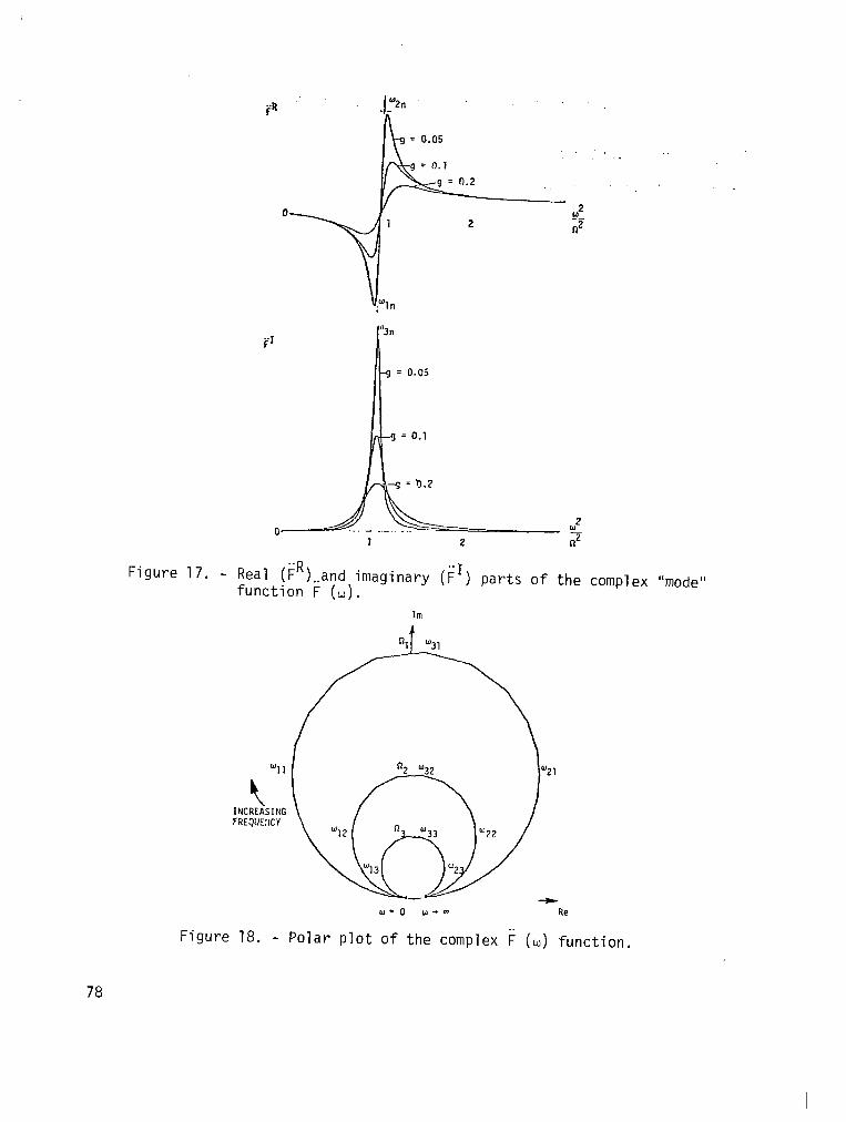
Figure 17. -

. . FI

Real (kR)..and imaginary (FI) parts of the function F (w).

Im

INCREASING FREQIJK'CY

complex "mode"

Figure 18. - Polar plot of the complex 1 (w) function.

78

The 'iR (w) function is characterized by two peaks at

Yn = .'n (128)

and

W2n = Rn J 1 f gn2 + 9, /i-q ;

*- 1 / Q

(‘29)

((130)

while the F' (w) function has only one peak at ti3n = on /l + gnL .

Note that,

2 2 W2n - Yn

ori2 -= an /T

which increases with increasing damping.

From the plots in Figure 17, it is seen that linear combinations of iR and c1

vary rapidly in the vicinity of the natural frequency, and are either negligible

or slowly varying with frequency in the regions away from the natural frequency.

Separated Modes. - Equation (121) carries the basic implication that the

effects of the structure's modes occurring at different frequencies on the mea-

sured mobility are additive in the frequency domain. If a mode occurs at a fre-

quency, in the neighborhood of which the contributions from the other modes of

the structure are either negligible or are weakly varying with frequency, such

a mode is said to be well separated. The nature of the measured mobility in

this frequency range will be dominated by that particular mode.

Classical Modes. - In the case of a classical mode, i.e., when the system

mode shape is the same for the damped system as it would be for the undamped

system the A. Jkn

is a real number, i.e., A1 jkn = 0, and the real part of the mea-

sured acceleration mobility will show two turning points for each separated

mode and the imaginary part will show a single turning point only. For a

classical mode, equation (130) can be approximated to give an estimate of the

damping coefficient: g, = (m2n - uln)/an .

79

Figures 19 and 20 show acceleration mobility measurements obtained from a

helicopter structure. Two close, but distinguishable modes are present. The

dominant mode can be seen to be very nearly classical, with double turning

points in the real, and a single turning point in the imaginary mobilities.

Complex Modes. - For the general case of nonclassical or complex modes,

both Agkn and A1 jkn are significant. The measured real and imaginary mobilities

of a well separated mode contain linear combinations of both FR(w) and F1(w)

in proportions given in equations (122) and (123). In particular, if

AJkn " Agkn, it is the imaginary part of the acceleration mobility which will

show two turning points, while the real part will show a single turning point

only. Figures 21 and 22 show an example of this occurrence in the data measured

from the AH-1G (the shaking coordinate was vertical at the tail, and the mea-

surement coordinate was vertical at the nose) between 40 Hz and 50 Hz.

Coupled Modes. - System modes, occurring in frequency ranges such that

their mutual contributions to the measured mobility in this frequency range are

rapidly varying functions of frequency, are said to be coupled.

Mode Clusters. - A mode cluster (or a cluster of modes) is characterized

by a group of system modes which are coupled together by virtue of the prox-

imity of their resonances. Mode clusters are usually separated by regions of

negligible or slowly varying mobility values in the frequency domain.

Mode clusters generally have the appearance of single modes in wideband,

low frequency resolution mobility measurements. Higher resolution data usu-

ally helps to reveal the modal content of a particular mode cluster. Figure 23

shows broad band (0 - 200 Hz) mobility of a helicopter vertical tail shake,

measuring vertical acceleration at the nose. Between mode clusters, measured

mobility is seen to vary slowly close to the zero value. In fact, what appears

to be a single mode in the 0 - 10 Hz frequency range is actually a cluster of

two modes as Figures 19 and 20 (which are higher resolution measurements of .the

same mobility in the 5 - 10 Hz range) show.

80

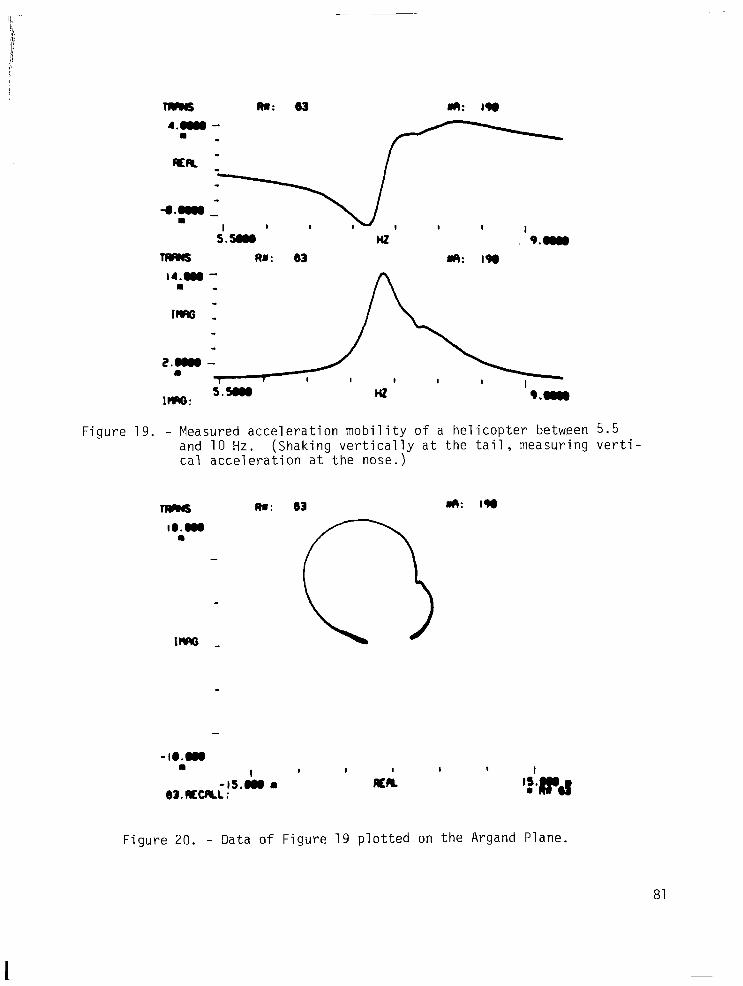
Ra: w 4.w -

l -

9.am RN: w 4R: I9a

t4.on 8

Figure 19. - Measured acceleration mobility of a helicopter between 5.5 and 10 Hz. (Shaking vertically at the tail, measuring verti- cal acceleration at the nose.)

-1O.W a

Ra: w 4R: I9e

I I I I I ,

I

-1S.k a AER 63.REcaL: ‘We!

Figure 20. - Data of Figure 19 plotted on the Argand Plane.

81

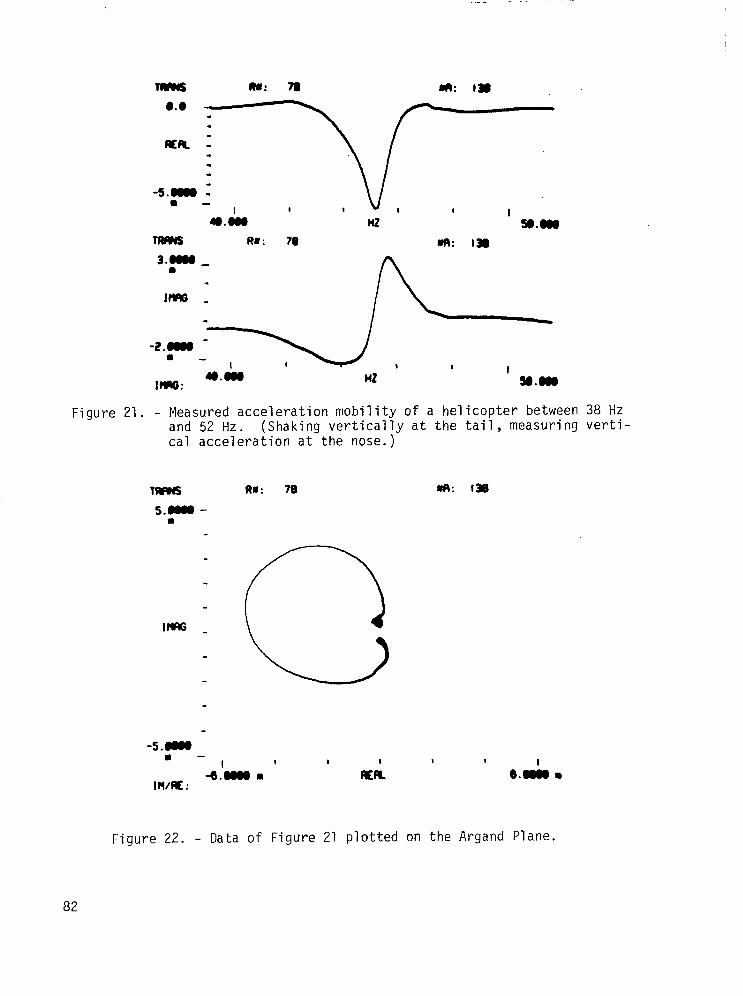
m . -

-5.am : a -

Y.ea

Rlr: 78 m: IS

3.m _ a

s I#0 -

a -

Figure 21. - Measured acceleration mobility of a helicopter between 38 Hz and 52 Hz. (Shaking vertically at the tail, measuring verti- cal acceleration at the nose.)

s.aa - l

-5.aa 8 -

I I I I I I I

4.8WO a RER e.aa 8 Ifl/fE :

Figure 22. - Data of Figure 21 plotted on the Argand Plane.

82

Figure 23. - Measured acceleration mobility of a helicopter between 2 Hz and 200 Hz. (Shaking vertically at the tail, measuring vertical acceleration at the nose.)

Identification of mode clusters is useful in determining which modes

should be included when truncating equation (121), since the contributions of

the remaining modes are either negligible or frequency independent. It also

helps in identifying frequency segments for higher resolution data acquisition.

Shake Testing for Global Parameters

Each elastic mode of the structure is characterized by a natural fre-

quency on and a damping coefficient gn which are global properties of the struc-

ture. These are the only constants that enter into the mode frequency functions.

They are the same for a given mode, regardless of the response coordinate. The

first stage of modal testing is to determine the global parameters of the domi-

nant elastic modes which occur inside the frequency range of interest.

83

I -

The experimental data required for determining the global parameters are

the continuous frequency plots of a number of mobilities which are considered

to represent the global vibrational behavior of the structure. For a selected

set of shaking locations, e.g., tail vertical, tail rotor gearbox lateral, etc.,

the transfer functions between the response coordinate and the shaking coordi-

nate are measured over the determined frequency range. Typical response coor- dinates for such measurements are: (1) nose vertical; (2) wing (right and/or

left) vertical; (3) center of gravity vertical; (4) tail vertical; and

(5) horizontal stabilizer vertical.

The test set up for measuring frequency dependent mobility functions is

shown in Figure 24. The helicopter is suspended as a free body by soft rubber

bungee chords. The configuration shown has the shaker located vertically at

the tail and the response accelerometer at the horizontal stabilizer vertical.

Signals for driving the electromagnetic shaker originate from the signal gener-

ator. A force gage, installed at the point of force application generates

voltage signals which are proportional to the applied force. These signals are

inputs to the dual channel digital signal analyzer. The accelerometer at the

response coordinate generates voltage signals, proportional to the response

acceleration, which are also inputs to the digital signal analyzer.

The signal analyzer is capable of sampling the time-domain force and

response signals, digitizing these samples and computing the real-time Fourier

transforms of the data. It also computes the least squares estimate of the

frequency-domain transfer function between the input and output spectra, which

is the mobility between the response and forcing coordinates. All the fre-

quency functions computed by the analyzer over the specified frequency interval

can be stored on cassette tapes for future restoration and analysis. The

oscilloscope allows the monitoring of the time-domain signals emanating from

the force and response transducers. The frequency counter is used to precisely

measure the frequencies of harmonic signals when required.

The accuracy with which the global parameters can be estimated is criti-

cally dependent on the quality of the data acquired for this purpose. For each

pair of force and response locations, a random shake is done with the frequency

84

RUBBER BUNGEE CHORDS

DIGITAL

ANALYZER

FREQUENCY COUNTER

SIGNAL GENERATOR

Figure 24. - Schematic of test set-up for global parameter testing.

85

bandwidth set to span twice the frequency range of interest (in this case,

0 - 200 Hz, since the modes of interest are between 2 - 100 Hz). This is done

to insure that the modes up to 100 Hz are not coupled to modes occurring beyond

100 Hz, as may be the case when a local mode is present. For each new shaking

station, several force levels are tested until the range of applied force is

reached where the mobility plots do not depend on the force level anymore.

This is one of the linearity requirements on the mobility plots. Having estab-

lished the required force level and the absence of local coupling modes at

higher frequency, another random shake is done, this time with the bandwidth

set at 2 - 100 Hz. The above procedure is repeated for all the accelerometers

which have been selected for global parameter testing.

The ratio of modal acceleration coefficient to damping (A jkn/gn) varies not only from mode to mode, but also from mobility to mobility, for a given

mode, and the prominence of the various modes of the structure will be different

in each of the mobilities recorded. That is to say, a given mode i occurring

at oi may appear very prominently on mobility ijk(w), while the same mode may . .

not be so significant in the mobility Yje(m), where 9, designates a response

coordinate different from k. This will especially be the case if the mode shape

associated with mode i has a much larger mode element at coordinate k than

coordinate II. The prominence of a mode may also be due to light damping. Thus,

by examining the set of broadband mobilities recorded, it is possible to asso-

ciate each mode i with the mobility where the mode most prominently appears.

Although it is possible to obtain rough estimates of the natural frequen-

cies and damping of the structural elastic modes from these broadband mobility

plots especially when damping is very light (e.g., peaks of the imaginary

mobility plots, and frequency separation of the peaks in the real mobility

plots), there are a number of specific considerations why broadband mobility

data is not suitable for global parameter extraction. Among these considera-

tions are:

Measurement Accuracy. - The low frequency resolution associated with broadband

mobility measurements tends to introduce errors into the measured mobility

values due to the phenomenon of leakage. Leakage has to do with a spreading

86

of the energy contained at each discrete frequency over a relatively narrow

band nearby. Although considerable effort is exerted into reducing leakage

effects (e.g., by appropriately windowing) by the equipment manufacturers, the

phenomenon still has to be reckoned with when the frequency resolution gets

below certain limits. For acceptable measurements, bandwidths of about 25% of

the center frequency have been recommended.

Parameter Extraction Accuracy. - Also associated with low frequency resolution

are inaccuracies in the parameter extraction methods due to the frequency

spacing between successive data points. The polar plot of mobilities, (see

Figure 18) in the vicinity of a mode, describes a circular arc. Most methods

for extracting natural frequencies, damping and modal acceleration coefficients

are based on fitting a continuous circle through measured data and in some

cases computing the rate of change of the arc length with frequency. Since the

frequency data is discrete, arcs of the circle are necessarily approximated by

segments. The error incurred by approximating a circular arc by a straight

line segment increases as the frequency spacing between successive data points

increases. Narrow band data, with bandwidth less than 25% of the natural fre-

quency of a given mode, have been found to yield sufficiently accurate results.

Initial estimates of the natural frequencies can be obtained from the broadband

data.

For sufficient frequency resolution and to m

bandwidths are recommended for use in narrow band

signal analyzer.

inimize leakage, the following

testing using the HP5420A

87

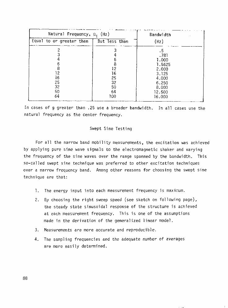
Natural Frequency, fii (Hz)

Equal to or greater than 'But less than

2 3 4

i 12 16

:; 50 64

: 6

1: 16 25

;; 64

100

Bandwidth

(Hz)

.5

.781 1.000 1.5625 2.000 3.125 4.000 6.250 8.000

12.500 16.000

---

In cases of g greater than .25 use a broader bandwidth. In all cases use the

natural frequency as the center frequency.

Swept Sine Testing

For all the narrow band mobility measurements, the excitation was achieved

by applying pure sine wave signals to the electromagnetic shaker and varying

the frequency of the sine waves over the range spanned by the bandwidth. This

so-called swept sine technique was preferred to other excitation techniques

over a narrow frequency band. Among other reasons for choosing the swept sine

technique are that:

1.

2.

3.

4.

The energy input into each measurement frequency is maximum.

By choosing the right sweep speed (see sketch on following page),

the steady state sinusoidal response of the structure is achieved

at each measurement frequency. This is one of the assumptions

made in the derivation of the generalized linear model.

Measurements are more accurate and reproducible.

The sampling frequencies and the adequate number of averages

are more easily determined.

88

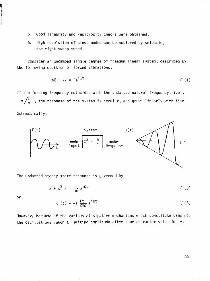
5. Good linearity and reciprocity checks were obtained.

6. High resolution of close modes can be achieved by selecting

the right sweep speed.

Consider an undamped single degree of freedom linear system, described by

the following equation of forced vibrations:

rni + kx = Fe iwt (131)

If the forcing frequency coincides with the undamped natural frequency, i.e.,

the response of the system is secular, and grows linearly with time.

Schematically:

System

The undamped steady state response is governed by

j; + Q2 x = F int me

or, Ft x (t) = -i 2mn e int

(132)

(133)

However, because of the various dissipative mechanisms which constitute damping,

the oscillations reach a limiting amplitude after some characteristic time T.

89

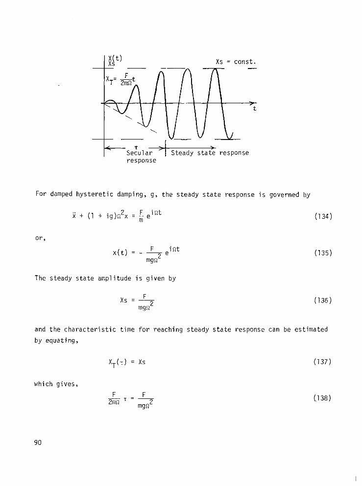
Xs = const. -

/ t

SeZular Y

1 >

Steady state response response

For damped hysteretic damping, g, the steady state response is governed by

F int ii + (1 + ig)n2x = m e

or,

x(t) = - --!-- e int

mgn2

The steady state amplitude is given by

xs = F

mcw2

(134)

(135)

(136)

and the characteristic time for reaching steady state response can be estimated

by equating,

XT(T) = xs (137)

which gives,

F F XT=-

mgn2

90

(.138)

thus: 2 1

T = gn= lrgf (139)

Suppose there are two neighboring structural modes with the natural frequencies

separated by af Hz. To resolve these two close modes, the speed at which the

excitation frequency is changing must be of the order of:

V = VA f = ngf Af Hz/set (140)

where g = damping coefficient (lower bound)

f = frequency in Hz

Af = mode resolution in Hz.

If an estimate of the lower bound of the damping coefficient and the required

sine shake mode resolution are available, the sweep speed required for swept

frequency, testing is directly proportional to the

i.e. 'h,) -- = const f

The relationship between the linear sea

signal generator is:

le and the logarithmic sea le on the

fdec fhz

= log10 f0 (142)

where

fhz = frequency in Hertz; (f0 5 fhz 2 10f 0)

fdec = frequency in decades; (0 5 fdec 2 1.0)

f. = base frequency on the scale.

From equation (142)

(141)

fhz = f. x 10 fdec (143)

91

dfhz Sweep speed v = - = - dfdec

dfhz dfdec Hz,sec ____ dfdec ' dt .

From equation (143)

dfhz - = (f. Rn 10) x 10 fdec

dfdec = fhz Rn 10

and

(144)

(145)

(146)

Thus, by selecting a constant logarithmic sweep speed (dfdec/dt = const. = a),

equation (141) is automatically satisfied.

The constant ~1 is determined by substituting the desired value of ?- into

equation (146). For example, fhz

if at 2 hz we desire a sweep rate of 0.07 Hz/set,

then

CL = 0.01(60) 2an 10 dec/min = .13 dec/min (147)

Estimation of Global Parameters

Various techniques have been developed for estimating the natural frequen-

ties and damping coefficients of the elastic modes of a structure from mobility

data. In all cases, certain assumptions have to be made about these modes.

The simplest case is when the mode is well separated and lightly damped. For

such modes, the natural frequency can be approximated by the peak of the imag-

inary displacement mobility. The damping coefficient can be estimated as:

(148)

92

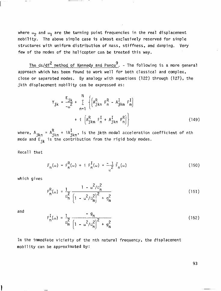
where w2 and W, are the turning point frequencies in the real displacement

mobility. The above simple case is almost exclusively reserved for simple

structures with uniform distribution of mass, stiffness, and damping. Very

few of the modes of the helicopter can be treated this way.

The ds/df* method of Kennedy and Pancu'. - The following is a more general

approach which has been found to work well for both classical and complex,

close or separated modes. By analogy with equations (122) through (127), the

jkth displacement mobility can be expressed as:

E. Y.

Jk =Jk+

2 -w Agkn F; - AJkn F;]

ti A!jkn F; + A;k,, F; (149)

where, A. Jkn

= AR jkn

t iA jkn' is the jkth modal acceleration coefficient of nth

mode and E. Jk

is the contribution from the rigid body modes.

Recall that

and

F,(W) = F:(M) + i F:(W) = 3 i',,(w) w

which gives

l- u2/n2

1 - 2/,2 2nt g2 n 1 n

(150)

(151)

(152)

In the immediate vicinity of the nth natural frequency, the displacement

mobility can be approximated by:

93

-

In equation (153), the sum of the contributions from all other modes has been

ight line: represented by a camp lex stra

CR n

(153)

t i Cf, 1

f$-t dz t i d,!,

Dropping the subscripts j, k, n and writing the real and imaginary parts of the

displacement mobility separately, gives

y1 (w cx Q) '- AR &,) t A1 FR(w) + C1 2 + dI Q2

(154)

(155)

If the nth mode is classical and well separated, the imaginary part of the modal

acceleration coefficient vanishes and the contributions from other modes are

nearly independent of frequency. In other words, AI, CR, and C1 vanish. Thus,

YR (w = n) = AR FR(w) + dR

Y1 (w = n) = AR F1(w) + d1

The peak of the imaginary mobility occurs when

or,

I s = 0 = AR 4 dw dw

Q2 [[l - U%2]2 t g*]2

(156)

(157)

(158)

(159)

94

which is when w~/Q.~ = 1, as stated previously.

The peaks of the real displacement mobility occur when,

or,

dYR - = 0 = AR + dw 2

dw

L J

which gives peaks at

and

or,

2 9

n2=1-g

2

3- l+g

= 0

(160)

(161)

(162)

(163)

(164)

as stated previously.

When the mode is complex, equations (154) and (155) indicate that both the

real and imaginary parts of the displacement mobility contain linear combina-

tions of FR(~), FI(m), LO', and constants. The peaks in the mobilities in the

general case may not be simply related to the natural frequency and damping

coefficients. Naturally, different degrees of approximations are feasible,

depending on how complicated the situation really is.

A general technique, which has been found applicable to the majority of

modes encountered on the AH-1G helicopter is based on the rate of change of the

arc length of the modal curve (plotted on the complex plane, i.e., the plot of

the Y1 against YR with frequency as a parameter).

95

-;/pgqg d(u2) (‘65)

where s is the arc length.

The rate of change of the arc length with respect to the square of fre-

quency is stationary when

or

OR ___ + d2YR dY1 d2Y1 --=

d(w*) d(w')' d(w2) d(w*)'

0

(166)

(167)

Upon substitution of equations (154) and (155) into equation (167) and simpli-

fying, the following condition for the peak of the ds - plot is obtained:

c&d*

AR&-+AI~ ~0 d(w*) d(w*)

where \A/* z (AR)' 2

+ (A') .

(‘68)

For a well separated mode, the constants CR and C' will be nearly zero and

equation (168) gives

96

d

d(u2) (‘69)

Equation (169) does not involve the modal acceleration coefficients AR and A'.

Thus, the condition for the peaking of the rate of change of the arc length

with respect to frequency squared, holds true regardless of how complex the

mode is, as long as it is well separated.

Equation (169) can be expanded, making use of equations (151) and (152),

and the result is:

d

d(u*)

[[, ~~]2-g~]2+4g~ 1 -$q2

2[[1 - $I2 + gj4

L

Equation (170) can be evaluated to yield

d

d(u2) = 4

Jo

=o

2

[ - 1 - ;2

il 1

1 -it- t QE

- = 0

1 3

g2

(170)

(17’ 1

J

Thus, for a well separated mode, the peak of the ds - plot will occur at the

d(u2) natural frequency, regardless of whether the mode is complex or classical. Any

suitable finite difference scheme can be used to compute ds - from measured

data using equation (165). db2)

It turns out that even for modes that are not well separated, the peaks ds of the -

6') plot still give good approximations to the natural frequencies.

To establish why this is so, consider equation (168) term by term. The first

term vanishes at the natural frequency, as we have already seen. The remaining

terms can be rearranged as:

97

At the natural frequency

d2FR ___ =

d(w')'

0

the remaining term becomes

_ ?-- [$/JR - CR/$] fi8g3

Lightly damped modes generally tend to be classical and well separated. This

is understandable, since in the limit of zero damping, a classical undamped

mode results. Thus, the low damping which will tend to drive 2/n8g3 up, also

drives [CIAR - CRA1] down, effectively neutralizing the expression. This con-

sequently reduces the error incurred by approximating the natural frequency by

the peak of the ds/d(w') plot. Experience has shown that modes which are too

close to be resolved by the ds/d(w') routine may not be resolvable by any other

method presently known.

The diameter of the modal c ircle that fits the curvature of the d isplace-

ment mobility plot (on the polar plane) in the vicinity of the natural fre-

quency is:

(‘72)

(173)

(174)

At the natural frequency;

dYR --ARtc

d(02) U=R g2fi4 iI2 (175)

98

and +

dY'

d(u2)

Substituting equations (175) and (176) into equation (165) gives

ds

d(u2)

The plot of arc length

the sketch, below:

By fitting

obtains a,

From equat ions (174) and (178), the damping coefficient is evaluated as:

g = D/an2 (179)

where D is the diameter of the circle fit to the mobility data, a is the gra-

dient of the line fit to the S plot and R is the natural frequency.

S

_ - A1 + C1 w=R !J2Q4 2

JAI

= -+ Error of approximation w=R g2fi4

('76)

(177)

s against LO' has a characteristic S shape, as shown by

A / Region around natural frequency

2 w

the best straight line to the inflection region of the S curve, one

the gradient of this line.

a = lA1/g204 ('78)

99

Testing for Orthonormal Modes and Mode Shapes

The mode shapes of any structure are related to the modal acce

coefficients as shown in equation (118); i.e.,

lerat i

A. =& Jkn n jn +kn

where $. Jn

and $kn are mode shape elements at the jth and kth coordinates

on

(‘80)

of the

nth mode; mn is the generalized mass of the nth mode. There are two basic

types of orthonormal modes which can be distinguished by considering the nature

of the response and the excitation. The ordinary vibration orthonormal mode

element, Y, has units of (l/mass)"'. The products of the jth and kth ortho-

normal mode elements and the mode frequency function summed over the modes

defines the jk vibration mobility. On the other hand, the strain orthonormal

mode element, y(E), has units of the square root of the reciprocal of

force x seconds' x length. The products of the jth strain and kth vibration

orthonormal mode elements and the mode frequency function summed over the

modes defines the jk strain mobility. The types of orthonormal modes used in

analytical testing and the corresponding types of mobilities are summarized

in Table XVIII.

TABLE XVIII. - SUMMARY OF MOBILITY AND ORTHONORMAL MODE ELEMENTS

L

100

Mobility

anq * J aAfk

Wj

aAfk

Modal acceleration (Residue)

yk/“’ - Y. J

(E - Y. J

> yk/“’

Units of modal acceleration

length/force

l/force

length/force

length/force

-

The orthonormal mode elements are defined as:

and

Y 1

kn ' r @kn n

I Thus,

and

A jkn = 'jn 'kn

A jjn = lyjn12

It follows from equations (183) and (184) that

A jkn 'kn = JA----

jjn

It can also be deduced that

Vlkn = f /5$i$

(‘81)

(‘82)

('83)

(184)

('85)

(186)

The choice of using either equation (185) or equation (186) to determine ykn

depends on the accessibility of the modal acceleration coefficients involved.

Note that two shaking stations are involved in equation (186), whereas only one

shaking station is involved in equation (185). It may turn out that the

driving-point data that yields Ajjn are such that accurate estimations of the

A jjn for a number of the modes are not easy. This may in part be due to a

strong local mode coupling, or a residual effect. In cases where this is so,

it may be better to shake at a number of coordinates, and then use schemes

similar to that in equation (186).

Consistency of the phase angle in equation (186) is achieved in the fol-

lowing manner. For an orthonormal mode element, in the nth mode, of large mag-

nitude, say ylkn, let

101

ykn = /II ajn i

: ($jkn ' $akn - 'ejn)

where $I is phase angle. For any other orthonormal mode element, say p,

'pn = e

Mode shapes of the structure, normal

element can be obtained directly from the

ized w

modal

ith respect to the highest mode

acceleration coefficients as:

1 A.

J mm

'A jln

'Aj2n

\ jNn/

. .

A'

- $kn)

(‘87)

(‘88)

(‘89)

where A. j,max,n

is the modal acceleration coefficient with the maximum amplitude

in the column corresponding to the nth mode, when shaking at the jth coordinate.

The generalized mass, corresponding to the mode shape thus normalized is com-

puted from equation (180) as:

m =9 n jn 9kn'Ajkn = AjIjn'(Aj max n)' , , (‘90)

In order to obtain the elements of the orthonormal modes and mode shapes,

the modal acceleration coefficients of all the modes for the mobilities

relating the response coordinates to the shaking coordinates have to be deter-

mined. The computational scheme for determining the modal acceleration coef-

ficients requires mobility data at discrete frequencies. The technique, herein

referred to as the matrix difference method, was developed by F. D. Bartlett,

Jr., of the Structures Laboratory, USARTL (AVRADCOM). The matrix difference

method is well suited to processing large numbers of transducers for modal

analysis using multiplexing data acquisition systems common in the helicopter

industry. The natural frequencies and modal damping must be determined before-

hand.

102

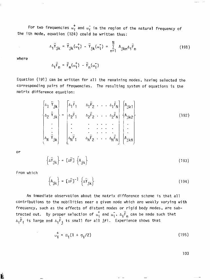
For two frequencies of and UT in the region of the natural frequency of

the ith mode, equation (124) could be written thus:

A3 I jk - 'jk(uf) = ; A. "

n=l JknAiFn

where

Aif,, = $,(w;) - /&$

Equation (191) can be written for all the remaining modes, having selected the

corresponding pairs of frequencies. The resulting system of equations is the

matrix difference equation:

or

From which

. .

'1 'jk . .

'2 'jk

.

. . .

'N 'jk

=

. .

AIFl . .

A2F1

.

.

. .

'NFl

. . . . AlF2 . . . AIFN

. . . . A2F2 . . . A2FN

. . . . .

. . . . .

. . . . . . . . .

'NF2 ' - ' 'NFN

A. Jk'

Ajk2

A. JkN

(192)

(‘93)

An immediate observation about the matrix difference scheme is that all

contributions to the mobilities near a given mode which are weakly varying with

frequency, such as the effects of distant modes or rigid body modes, are sub-

tracted out. By proper selection of C,J; and w;, AiFn can be made such that

Aifi is large and A.?. is small for all j#i. 1 J Experience shows that

t w.

1 = 'it' + gi/Z) (‘95)

103

and W.

1 = n.+l - gji2) (196)

are the most effective choices for the upper and lower discrete frequencies.

For these discrete frequencies, the matrix [A;] is well conditioned for inver-

sionsince the off diagonal terms are small compared to the diagonal terms.

Test procedure. - Figure 25 shows the schematic of the instrumentation

set-up for the shake test for orthonormal modes and mode shapes. Signals from

all the accelerometers and from the force gage are transmitted via telemetry

to a computer where the transfer functions between the response coordinates and

the force coordinate are computed and printed out. The excitation signals are

sinusoidal at the discrete frequencies W; and CO; for i = 1, 2, . . . N. The

same force levels used for the swept sine global parameter shake test are also

used for the modal shake test at the corresponding discrete frequencies.

Derivation of Mobilities

Underlying any technique of modal analysis is the principle of linear

decomposition of structural response mobility into contributions from the natu-

ral modes occurring between a chosen frequency interval. The preceding methods

estimate not only the natural frequencies and damping coefficients of each

mode, but also the modal acceleration coefficients of each modal contribution

to the mobility between response and forcing coordinates.

Subsequent to the determination of the modal parameters and modal con-

stants, the next logical step is to reconstruct mobilities both between a pair

of forcing and response coordinates over a continuous frequency interval, and

at a chosen frequency between several pairs of forcing and response coordinates.

By comparing the mobility derived over a continuous frequency range with the

measured mobility over the same frequency range, some assessment of the accu-

racy of the global parameter estimations can be made. The comparison of dis-

crete frequency mobilities for a large number of coordinate pairs allows the

assessment of the acceptability of the orthonormal mode and mode shape calcula-

tions. The results of these comparisons build the confidence in the mobilities

which are derived but not actually measured.

104

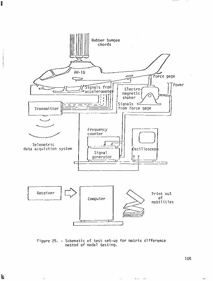
I/// iii I i r i Rubber bungee chords

Telemetric data acquistion system

CI

Frequency counter

L F-

r----- I

l-----r’ /(I, Pscilloscop

L 1 >

1. Signal generator

0 I-J Ip P

0 L: t - J

’ I L I

0 Computer

& s.d -- -- , I 1

I 1 ,

I 1

Print out Of

mobilities

Figure 25. - Schematic of test set-up for matrix difference method of modal testing.

105

-

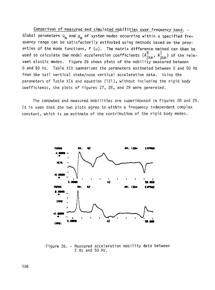
Comparison of measured and simulated mobi.lities overfrequency band. -

Global parameters an and g, of system modes occurring within a specified fre-

quency range can be satisfactorily estimated using methods based on the prop-

erties of the mode functions, F (w). The matrix difference method can then be

used to calculate the modal acceleration coefficients (Aikn, AJkn) of the rele-

vant elastic modes. Figure 26 shows plots of the mobility measured between

0 and 50 Hz. Table XIX summarizes the parameters estimated between 0 and 50 Hz

from the tail vertical shake/nose vertical acceleration data. Using the

parameters of Table XIX and equation (121), without including the rigid body

coefficients, the plots of Figures 27, 28, and 29 were generated.

The computed and measured mobilities are superimposed in Figures 28 and 29.

It is seen that the two plots agree to within a frequency independent complex

constant, which is an estimate of the contribution of the rigid body modes.

s.Biw IQ

WI: Bz m: 1334 Em

Figure 26. - Measured acceleration mobility data between 2 Hz and 50 Hz.

106

TABLE XIX. - ESTIMATED PARAMETERS BETWEEN 0 - 50 Hz (TAIL VERTICAL SHAKE, NOSE VERTICAL .ACCELERATION)

Natural frequency Damping

lode No. coefficient

n "n (Hz) gn

1 7.33 0.062 .165

2 8.09 0.12 .102

3 13.3 0.13 - .004

4 15.97 0.085 .005

5 16.35 0.05 .012

6 17.63 0.08 .031

7 22.1 0.15 - .017

8 28.4 0.11 - .024

9 40.7 0.12 .002

10 45.3 0.026 .009

T Nose/tail modal acceleration coefficient

Real

AfN ZT n , ,

g/l000 N

Imagi nary I

AZN, ZT, n

g/l000 N

.032

- .081

- .OOl

.032

0

- .013

- .092

.026

- .005

.032

i.0 lu s&m TRms A#: 581 m: I6

Figure 27. - Numerical simulation of the elastic component of the acceleration mobility data.

107

,,,,,, ,,,...-.- . ,..,.,,--- . . . . ,.-.. , ,, , ., , . ,-, ,.., ,,,. __,._.-._-.-_-._ . . . . . . . . _.._ . . . . ..- -.. . . _.. . . . ..__..--.. .

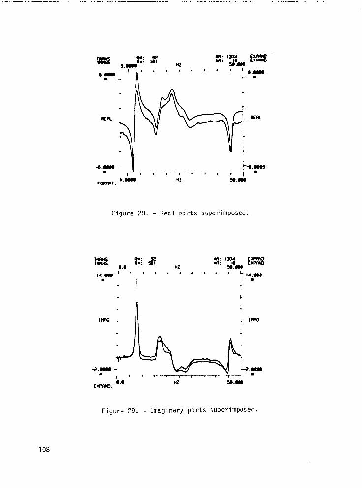
+8!48 I-‘ l---T- -1 7 I .

n2 a A

4.8888 - . , I I-’

Figure 28. - Real parts superimposed.

Figure 29. - Imaginary parts superimposed.

108

Modal Series Method. - Equation (121) can be rewritten in the following

form:

;ijk = Ejk + RL N

j,(m) + ,El Ajkn 'n(w) + Rrk(") (197)

where Rik(w) is the low frequency mobility residual; i.e., contribu-

tions to the mobility by elastic modes which occur at fr

Rrk(w) is

The rigid body acce

weights data. 5

'quencies below the lower test frequency limit.

the high frequency mobility residual.

eration coefficient, E. Jk’

is determined from geometry and

If the lower test frequency limit is near zero, it follows that RL = 0.

The higher test frequency limit is usually selected high enough so that RH can

be safely assumed to vanish for all but certain driving-point mobilities which

may suffer either from local mode effects or from high frequency mode residuals.

When all the global modal parameters (natural frequencies and damping coef-

ficients) and the modal acceleration coefficients have been determined (see

Table XX), the acceleration mobilities between pairs of motion coordinates which

do not include the shaking coordinate can be computed from:

. . Y Em = E Rm

t ; Ay;/kn Fn (a) n=l

(198)

where k is the coordinate of the shaking station for the data which generated

A ak and Amk* It is necessary to select the shaking station k such that there

is no local mode or high frequency residual effect on the estimated value of

If only Nk of the modes are well defined by shaking at k, while the

remaining Np modes are better defined by the shake at p, then

Nk A ;i,, = Et, + 1

kknAmkn .. NpA A

n=l Akkn F,(w) + 1

n=l "y mpn

wn i,(w) (199)

109

TABLE XX. - SUMMARY OF ESTIMATED MODAL PARAMETERS FOR AH-'IG HELICOPTER.

e

Rn 9, j Rn gn j

7.28 6.28 .07 .16

8.35 7.53 .08 .05

13.94 8.55 .06 .ll

21.48 14.35 .16 .18

---I-- 23.71 16.39 .ll .068

25.59 18.45 .31 .13

29.96 21.93 .13 .074

31.63 24.12 .l .108

29.38 .112

-

SPECIAL CONSIDERATIONS IN MODAL ANALYSIS

Shaking Locations

Nonlinearities such as gradually hardening stiffness and ankylotic stiction

are alleviated by using sufficient shaking force so that the mobility is inde-

pendent of the shaking force. The power input from the shaker is equal to the

power dissipated by the helicopter through damping and is proportional to the

product of the square of the shaking force and the imaginary velocity mobility

(or real acceleration mobility divided by frequency). Maximum motion for a

given shaking force occurs at shaking point locations of high mobility. These

are generally at structural terminations such as high on a fin, at wing tips

or the hub.

It is also important to shake in the vicinity of any possible local modes

of interest. Consider the case in which, for a given mode, ylj = .2 and yk = 2.0.

For shaking at j, Ajj = .04 and Akj = .40. The response near this natural fre-

quency may be unnoticeable at the driving point, j, but evident in the kj trans-

fer mobility which indicates that k, or a point near it, should be a shaking

point. In this example, Akk is two orders of magnitude larger than A... JJ

Once modal accelerations have been obtained for and among the stations at

which the aircraft is excited, one shaker at a time, all the modal accelerations

can be used simultaneously for the best estimate of the orthonormal mode ele-

ments. Although the number of shaking locations depends on many factors, it

appears that five or six should be sufficient for most helicopter uses. For

the jth motion coordinate and N shaker locations the absolute value

A. Yj = 51

+ Aj2 + ... ' AjN

JAl1 t A22 + . . . t 2 Al2 + 2 Al3 . . . + 2 A23 + ...

N

1 A I i=l ji I = (?OO >

111

ApI + lp21 + (q . ..I2

The phase angle of the jth orthonormal mode element is given by

(201)

If the ds/dfL method is used to obtain the modal accelerations at and

among the shaking locations and the matrix difference method for all modal

accelerations, then

I I 9 = --

All/g2 (202)

+ A22/g 2

+ . . . + 2 A12/g2 + 2 A13,'g2 t . . .

High Frequency Residuals

The authors discovered that high frequency (e.g., 400 Hz) local modes may

cause distorted translational mobility plots, with force shaking at low fre-

quencies (e.g., 10 Hz) at or near a driving-point on the AH-1G. Dr. Albert

Klosterman and Dr. Jason Lemon of Structural Dynamics Research Corporation

noted high frequency residual effects and found the means of correction in

testing a 1750 HP electric motor for the United States Steel Corporation. 10

Dr. David Ewins of the Imperial College of Science and Technology, London,

found the same cause and effect in rotational mobilities measured on a turbine

rotor. 11 The effect does not occur at all driving-points, but it is not uncom-

mon. It occurred in tail shaking and vertical shaking at FS 2400 on the AH-1G

as shown in Figure 30. It did not occur in hub shaking or shaking at the tail

rotor gear box on the AH-1G.

The effect is associated with shaking points of very small mass concentra-

tion and elastic extension as in the cantilever beam of Figure 31. In a heli-

copter these correspond to soft, but not weak points, as opposed to hard points

usually, but not necessarily, such as skin attachment points or tail skids.

In some cases of helicopter fuselage concern, the high frequency local

modes are inconsequential in engineering and should be ignored in modal

112

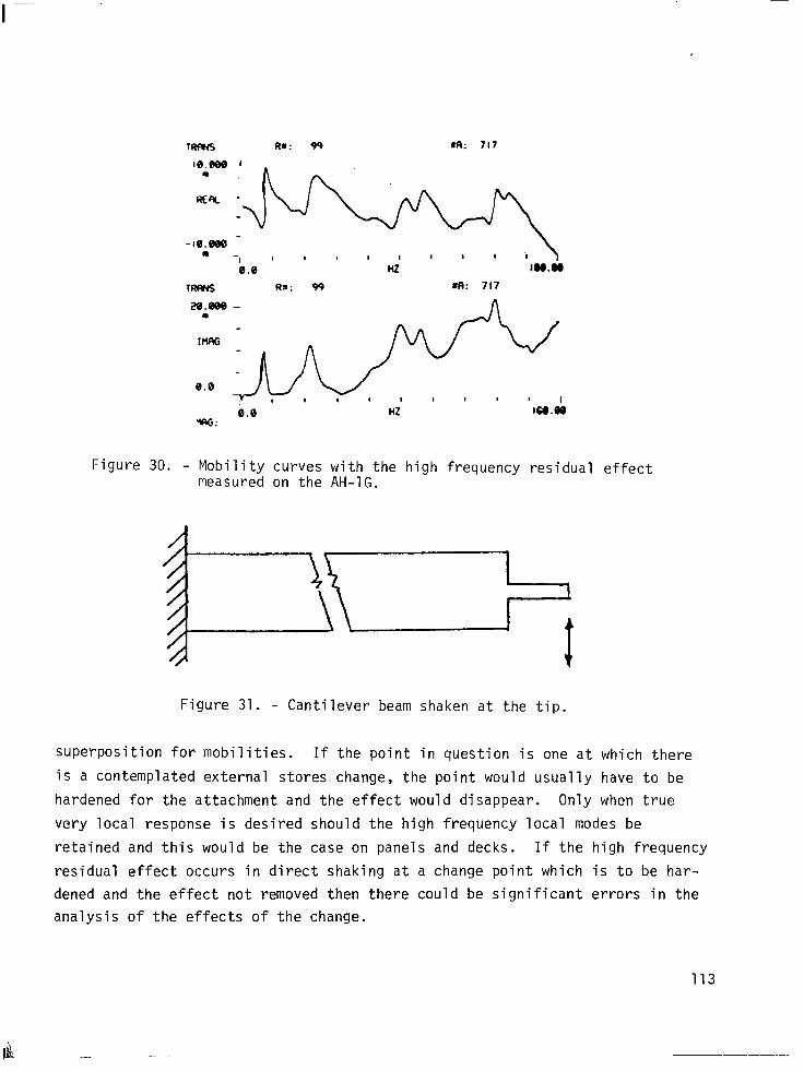
Figure 30. - Mobility curves with the high frequency residual effect measured on the AH-1G.

Figure 31. - Cantilever beam shaken at the tip.

superposition for mobilities. If the point in question is one at which there

is a contemplated external stores change, the point would usually have to be

hardened for the attachment and the effect would disappear. Only when true

very local response is desired should the high frequency local modes be

retained and this would be the case on panels and decks. If the high frequency

residual effect occurs in direct shaking at a change point which is to be har-

dened and the effect not removed then there could be significant errors in the

analysis of the effects of the change.

113

Figure 32 shows a simple chain having the residual effect. The natural

frequencies are at 4.95 Hz and 123.28 Hz, the latter being a local mode of the

small mass. The acceleration mobility from 1 to 10 Hz for the response at 1

due to force at 1, i(l,l) shown in Figure 33 shows the residual effect.

2kg

969 N/m 300 N/m

Figure 32. - Simple chain system with 5% structural damping.

0 5 10

Frequency, Hz

Figure 33. - Driving-point acceleration mobility at mass 1 of the chain of Figure 32.

v(l,l) is almost identical to v(l,2) and would be indistinguishable from

v(2,2), shown in Figure 34, if the local mode were removed. The slope of the

114

mobility from 4.8 to 5.07 Hz is virtually the same in Figure 33 as in Figure 34

and differential mobility parameter extraction methods, such as dS/df2 and the

matrix difference method, on the 4.95 Hz mode would be negligibly affected by

the residual effect. These methods can be used to accurately obtain modal

accelerations at driving points whenever the slope (dv/dw) resulting from high

frequency local modes is small compared to the max mum real or imaginary mobil-

ity slope at the natural frequencies of interest. The accuracy of parameter

extraction methods that are‘not of the differentia 1 mobility type is seriously

affected at driving points exhibiting the high frequency residual effect.

5

Frequency, Hz

Figure 34. - Driving-point mobility of mass 2 of the chain of Figure 32.

If the high frequency residual effect is to be retained there are two ways

to deal with it without shaking to very high frequencies. Because it is essen-

tially a driving-point phenomenon, one can shake at each of the driving points

having the effect and represent the effect as a flexibility term equal to the

constant difference between measured displacement mobility and the displacement

mobility synthesized over the frequency range of testing as shown by Klosterman

115

and Lemon", and Ewins". Alternatively, one could shake at only one point with

the points having the effect, and at which driving point mobilities are desired,

weighted by attached masses. The effect of the attached masses could then be

removed using the analytical testing equations as follows:

s the matrix of measured acceleration where Yrr mob lities at and among the

motion coordinates with the attached masses, mrr is the diagonal matrix of the

attached masses (in three spatial directions if necessary) and the parentheti-

cal superscript s meaning derived from modal synthesis over the frequency range

of testing.

‘I 11

22

33 [(.,I - b,,l-

. . .

i;,,(s) y2$s 1 y3$ >

. .

(203)

Effect of Damping Estimate Variations in the

Matrix Difference Method

The matrix difference method involves the difference between mobilities

above and below each natural frequency. Let wxl be the frequency below the

xth mode and wx2 be the frequency above the xth mode. For illustration pur-

poses let

wxl = /i? ~~ and wx2 = Jl+snx

where s is much less than unity. Then

AwX Aw, = wxl - wx2 =(R-JiG)n,=-s~~or-s=~

X

(204)

(205)

and in terms of displacement mobility:

116

N Ajki yjk(wxJ) - 'jk(wxz) = 1 2

gi gi

i=l giQi 2 - 2 wxl --+ig. 1 Qi2 '

- -t

!

let

qi gi Auxi •: 2 -

gj 2

1 wx2 - -t igi Qi2

Then, in matrix form

(206)

(207)

(208)

In view of equation (205), the xm th term in the CJAp matrix may be expressed

as

Au, fix2 --

- 2gM $2 x "M

2

gM "xM = c~.-~~ -

I

I

1 “x2‘2 Iax2 Au,‘~ 2

,X2 -- -- 2

"M , ,RM 2nx -gM ti2gr4 1 --

2

(209)

i "M ,

In the x row of the gAp matrix this term shows the coupling of the xth

mode with the mth mode when ratioed to the diagonal term g, a~,,. It will be

shown that: (1) when the modes are widely separated (i.e., for any mode x,

“X - 1 << (1 - 9,) fix and fix >> (1 + gxwl > fixLl and ~~ << (1 - gxtl ) fixtl and

i-2 xtl >> (1 + g,) Sax), then a frequency difference of Aw~/R~ = g, is preferred

in that it is least sensitive to errors in g; (2) for close modes, AuX/RX should

be less than g,; and (3) for Aw,/C2, much less than g,, the maximum error in the

diagonal term will be proportional to the error in g,.

Figure 35 shows a plot of the x row real part of the MALI matrix for hys-

teretic damping of 10% for various values of Aw~/L?~ equal to or less than

117

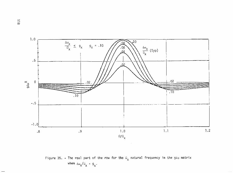
-1.01

..02

e

.lO

1.2

Figure 35. - The real part of the row for the fix natural frequency in the gall matrix

when Aw~/R~ < g . X

9, = .l. As seen from Figure 36, the imaginary part of the coupling of the x

mode with all other modes also drops off with decreasing Aw,/n,. This also occurs in Figure 35. Figures 37 and 38 illustrate the severe coupling effects

when Aw~/Q~ is greater than g by a large amount. Note the development of two

peaks when Aw~/M~ is .4 for g = .l in Figure 37.

The matrix difference method remains exact for values of Aw~/L?~ much

larger than g but the increased coupling with nearby modes tends to make the

gap matrix less well conditioned both physically and numerically.

As an illustration of the variation in coupling of two modes in the g

matrix with variation in Aw~/R~, consider a case of g = .l and fix2 = (1 - gM)"M2*

The following calculations are made for c$,, = 1.05409 and g = .l.

AWX/RX AwX 9Av

9 "X @ "PI @ Rx

2 .2 -946 68" -800 0"

1 .l .834 32" 1.000 0"

.8 .08 .697 75" .976 0"

.5 .05 .447 84" .800 0"

.2 .02 .180 89" .385 0"

.l .Ol .090 90" .198 0"

119

1.0' I ALL! 2<g AwX

.Q,- x gx = .lO

3

.a .9 1.0 1.1

R/Rx

Figure 36. - The imaginary part of the row for the fix natural frequency in the

CJAv matrix when Aw~/R~ < 9,.

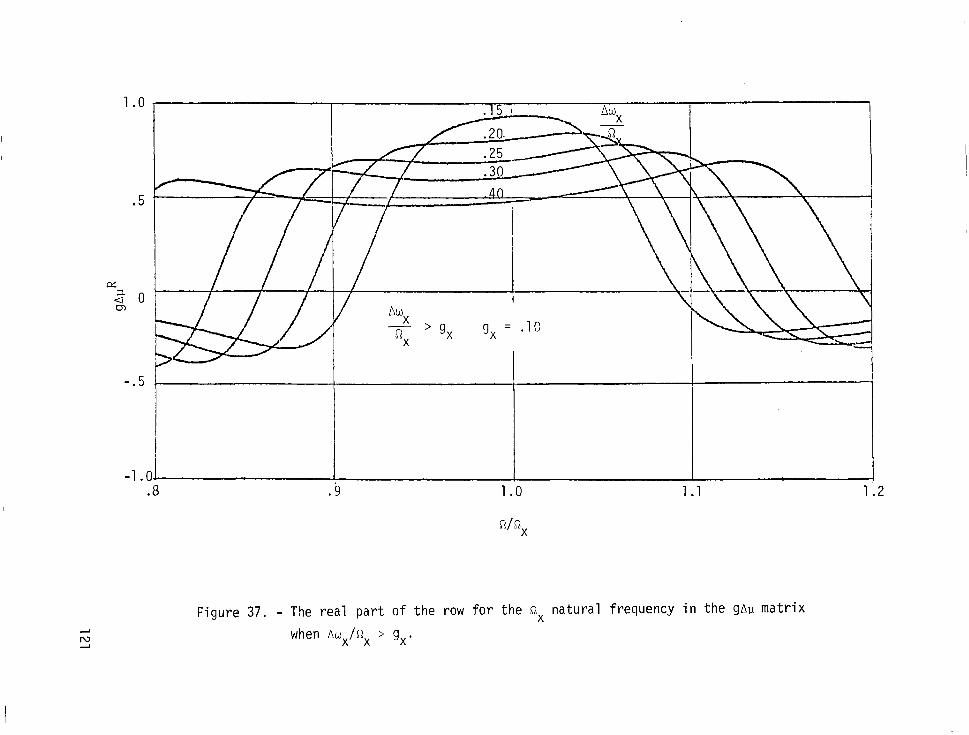
-. 5

I ,

-1.0 .a .9 1.0 1.1 1.2

Figure 37. - The real part of the row for the fix natural frequency in the gAu matrix

when Ao~/C$ > g,.

0 H 2 m

- .5

-1.0 .a .9 1.0 1.1 1.2

R/Rx

Figure 38. - The imaginary part of the row for the RX natural frequency in the

gAp matrix when Aw~/Q~ > g,.

If g were .Ol the same case of close modes has the following coupling

terms.

AWX/RX g

20 .2

10 .l

8 .oa

5 .05

2 .02

1 .Ol

.5 .005

Sensitivity to g

AwX

RX @ "M

.159 5"

.670 137"

.281 157"

.lll 166"

.037 168"

.018 168"

.009 169"

.lOO 0"

.i98 00

.246 0"

.385 0"

.800 0"

1.000 0"

.a00 00

When fix = "M the diagonal term from equation (209) reduces to

9, Al.lxx = %Ix AwXhX

2

+ 9x 2

(210)

As seen in Figure 39, the diagonal term in CJAp is least sensitive to the value

of g when awX/RX = g. In that vicinity a 4:l variation in g produces only a

f 10% change in the value of the diagonal term.

If Aw,/R, is very small in equation (210) compared to g then

AWX/RX 9, Au,, = + 2 y---

X (211)

and percentage errors in the diagonal term become proportional to percentage

errors in g.

123

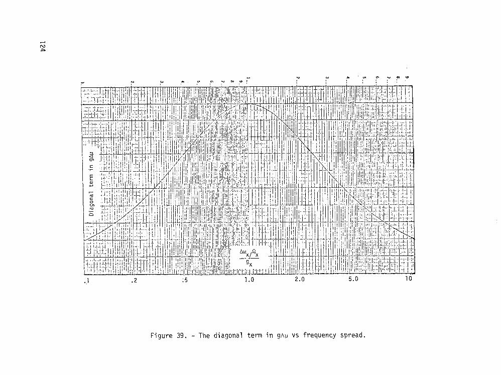
1 3 . I .L ;!I 1.0

Figure 39. - The diagonal term in ghp vs frequency spread.

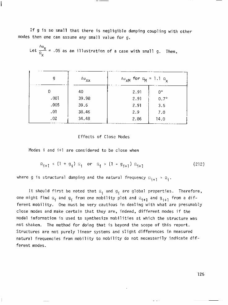
If g is so small that there is negligible damping coupling with other

modes then one can assume any small value for g.

Awx Let R = .05 as an illustration of a case with small g. Then, X

9

0

.OOl

.005

.Ol

.02

*'lxx

40

39.98

39.6

38.46

34.48

*uxM for op, = 1.1 ox

2.91 0"

2.91 0.7"

2.91 3.5

2.9 7.0

2.86 14.0

Effects of Close Modes

Modes i and it1 are considered to be close when

R i+l < t1 + !3i) “j or oi > (1 - g. ) o. 1+1 1+1 (212)

where g is structural damping and the natural frequency flit1 > oi.

It should first be noted that oi and gi are global properties. Therefore,

one might find oi and gi from one mobility plot and oi+l and gitl from a dif-

ferent mobility. One must be very cautious in dealing with what are presumably

close modes and make certain that they are, indeed, different modes if the

modal information is used to synthesize mobilities at which the structure was

not shaken. The method for doing that is beyond the scope of this report.

Structures are not purely linear systems and slight differences in measured

natural frequencies from mobility to mobility do not necessarily indicate dif-

ferent modes.

125

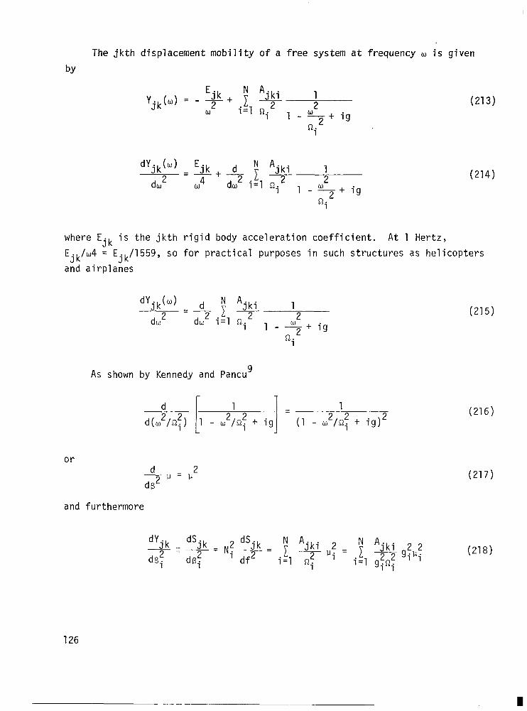
The jkth displacement mobility of a free system at frequency w is given

by

dYjk(W) dw

2 + ig

(213)

(214)

where Ejk is the jkth rigid body acceleration coefficient. At 1 Hertz,

Ejk/w4 = Ejk/1559, so for practical purposes in such structures as helicopters

and airplanes

or

+ ig

As shown by Kennedy and Pancu9

-u=lJ2 d

ds2

and furthermore

dVjk _ dS jk _ N2 dsjk _ F

dB; q F - .-- ' df2 i=l

= F Ajki 2 2 22 gi'i i=l gi"i

126

(215)

(216)

(217)

(218)

- -

Let dsjk - df2 i 1 be the value of dsjk - at the ith natural frequency.

df2 Then

and equation (218) can be -written as

or

A i I jki =

gfc2f

- Ii

g2P2 A.j ii cJ2Q2 ii I

(219)

(220)

(221)

a limiting case of the matrix difference method. It is not necessary for any i

di. that Jk be a peak.

df2 If the modes are not very close, as defined by equa-

tion (212), then the g2p2 matrix approaches the unit matrix. In any case, the

diagonal terms of the real g2p2 matrix will always be -1.00 and all other terms

will have an absolute value less than unity.

Defining

The orthonormal modal elements are obtained in the usual manner and any

mobility

Yam(") = - + t 2 'ai'mi gfPi w i=l

or, in terms of acceleration mobility

(222)

(223)

i\l ya,(w) = E,,, - co2 1 yaiyrni g&

i=l

127

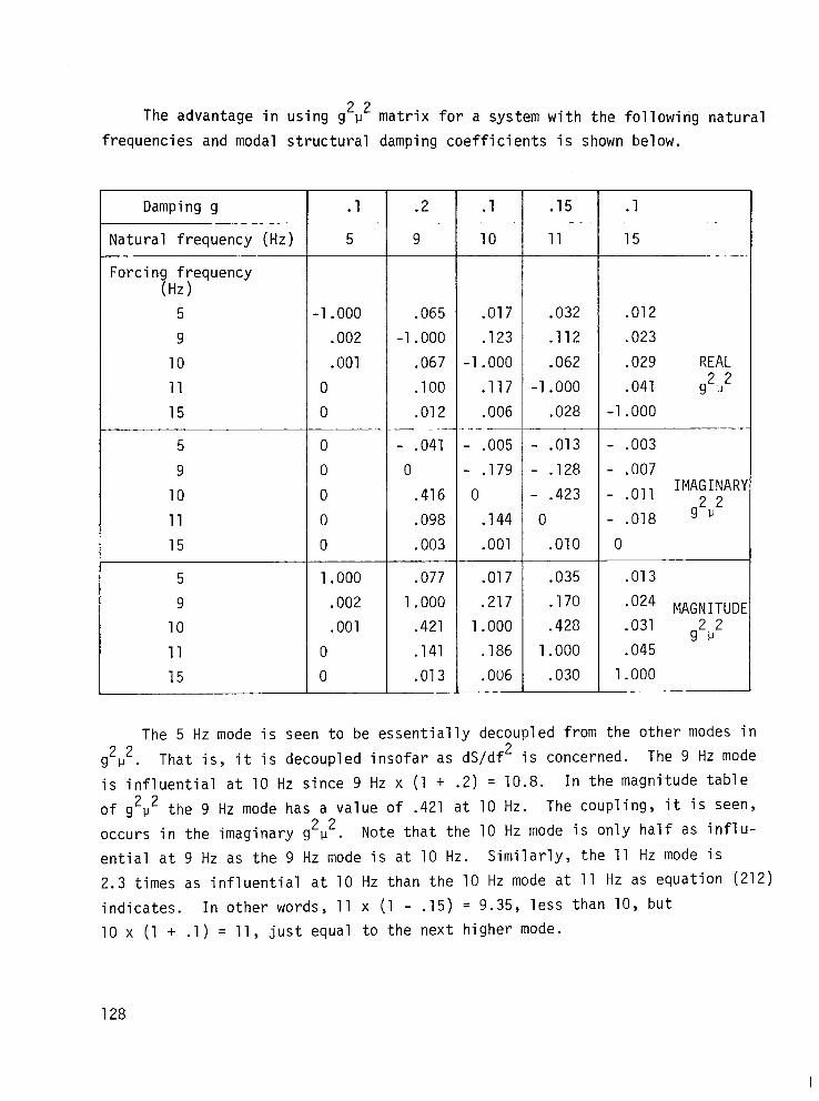
The advantage in using g2p2 matrix for a system with the following natural

frequencies and modal structural damping coefficients is shown below.

Damping g

Natural frequency (Hz)

Forcing frequency (Hz)

5

9

10

11

15

5

9

10

11

15

.l

5

-1.000 .065 .017 .032 .012

.002 -1.000 .123 .112 .023

.OOl .067 -1.000 .062 .029 REAL

0 .lOO .117 -1.000 .041 g21J2

0 .012 .006 .028 -1.000

1.000

.002

.OOl

0

0

.2

9

- .041

0

.416

.098

.003 _____

.077

1.000

.421

.141

.013

.l

10

.15

11

- .005 - .013

- .179 - .128

0 - .423

.144 0

.OOl .OlO

.017 .035

.217 .170

1.000 .428

.186 1.000

.OU6 .030

.l

15 -_

- -003

- .007

.Oll IMAGINAR'

- 22 - .018 ' '

0

.013

'o24 MAGNITUDI .031 g2P2

.045

1.000

The 5 Hz mode is seen to be essentially decoupled from the other modes in

g21J2. That is, it is decoupled insofar as dS/df2 is concerned. The 9 Hz mode

is influential at 10 Hz since 9 Hz x (1 + .2) = 10.8. In the magnitude table

of g2p2 the 9 Hz mode has a value of .421 at 10 Hz. The coupling, it is seen,

occurs in the imaginary g2p2. Note that the 10 Hz mode is only half as influ-

ential at 9 Hz as the 9 Hz mode is at 10 Hz. Similarly, the 11 Hz mode is

2.3 times as influential at 10 Hz than the 10 Hz mode at 11 Hz as equation (212)

indicates. In other words, 11 x (1 - .15) = 9.35, less than 10, but

10 x (1 + .l) = 11, just equal to the next higher mode.

128

.- -

The g2p2 matrix is clearly well conditioned. If the 9 Hz mode were,

instead, 9.9 Hz the .421 value in the magnitude table would become .999 at 10 Hz

and the value at 9.9 Hz from the 10 Hz mode would be .962 and the coupling

would appear mainly in the real matrix. The conditioning is worsened but not

necessarily unacceptable.

129

CONCLUDING REMARKS

Analytical testing provides a practical methodology for combining struc-

tural dynamic analyses with flight vibration performance. This report has pre-

sented analytical methods for evaluating the flight vibration and strain effects

of structural changes. The changed flight responses are characterized by the

dynamics of the change, original flight test data, and shake test data. Basic

analytical testing equations were derived to accommodate a category of changes

which included mass, stiffness, absorbers, and active vibration suppressors.

Illustrations of the analytical testing methodology were presented using

flight test and shake test data measured on an AH-1G helicopter. The applica-

tions were directed to the practical acquisition of helicopter vibration data

and the utilization of the method. Results of this investigation indicate the

possibility of combining flight data and shake test data with structural

changes in the helicopter airframe to predict the effects on flight vibrations

and strains. The results do not represent experimental verification of analy-

tical testing in any particular application.

Modal analysis based upon the measurement and past test processing of

transfer functions constituted a major part of the research associated with

analytical testing. The vibration testing procedures and modal analysis tech-

niques of the AH-1G were described. In addition, special considerations were

discussed to establish consistent data acquistion and to minimize problems

associated with modal analysis of complex structures.

130

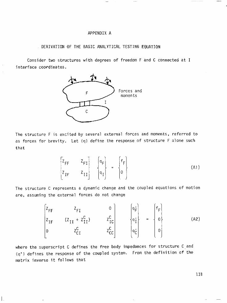
APPENDIX A

DERIVATION OF THE BASIC ANALYTICAL TESTING EQUATION

Consider two structures with degrees of freedom F and C connected at I

interface coordinates.

Forces and moments

The structure F is excited by several external forces and moments, referred to

as forces for brevity. Let Iq1

that

'FI

zII

define the response of structure F alone such

The structure C represents a dynamic change and the coupled equations of motion

are, assuming the external forces do not change

-'FF 'FI 0- I , I \

qk fF

'IF ($1 + z;+ ZC ,q;> = < OF

0 ZC CI z;: s;: 0 I / \ x

(A21

where the superscript C defines the free body impedances for structure C and

{q'l defines the response of the coupled system. From the definition of the

matrix inverse it follows that

131

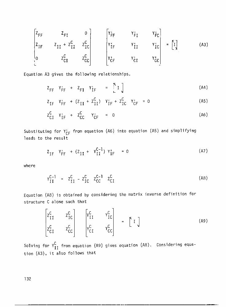
'FF

'IF

0 I-

‘FI 0

C zII + zII ZFC

Equation A3 gives the following relationships.

ion (A5) and simplifying Substitut ing for YCF from equation (~6) into equat

leads to the result

'FF y;-F •,- +I y;F = I II I

'IF YkF +- (ZII + z;+ ';F + ';C yCF

ZC C CI y;F + zcc yCF = 0

y;C

Yic = I 111

yk

=0

'IF y;rF t (zII + y&l) y;F = '

where

ye-l = zc C C-l II II - zIc zcc

Equation (A8) is obtained by considering the matrix inverse definition for

structure C alone such that

-C yII YC IC

C ycI YC cc

= r 1 I

Solving for YiI from equation (A9) gives equation (A8). Considering equa-

tion (A3), it also follows that

(A31

(A41

(A5)

(A6)

(A71

(A81

(A91

132

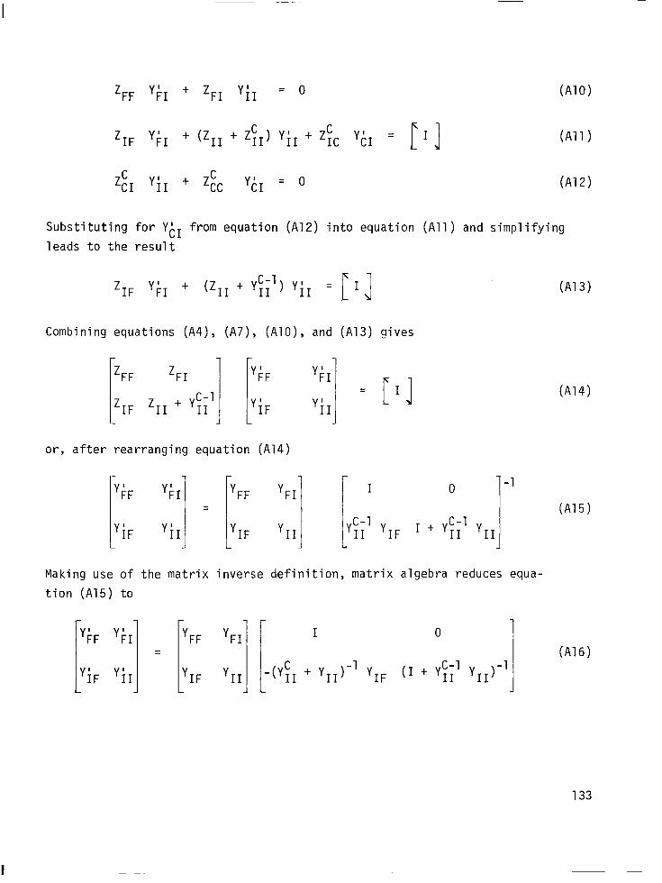
‘FF ‘;I + ‘FI ‘;I = 0 (AlO)

'IF ';I + (‘II + ‘II c > Y;* -I- zic Yi* = r I ] (All > i

C zcI y;I + ZFc yiI = 0 (A121

Substituting for Y& from equation (A12) into equation (All) and simplifying

leads to the result

'IF ';I + ('11 + '11 C-l) Yi* = [ I ]

Combining equations (A4), (A7), (Al 0))

1:; zI:~yy] 1::

or, after rearranging equation (A14)

'FF 'FI

'IF yII

and (A13) gives

y;-I

y;I

= c I I

I 0

' 'IF I + Y;;' YII

(A13)

(Al4)

-1

(A15)

Making use of the matrix inverse definition, matrix algebra reduces equa-

tion (A15) to

YII) -1

‘IF (1 t Y;;’ Y**)-l I

(A16)

133

or, y;F

C = 'FF - 'FI (YIr + y&1 'IF

Y;F = YIF - yII ty;I ’ ‘II)-’ ‘IF

(A17)

(AW

Since the external forces are on structure F, postmultiplying equations (A17)

and (A18) by the force vector yields

{qj = {q} - PqrJ [y:, + yI1J-l {qI} or, in a slightly different form

{q’} = (4) - [YqI] [I + yii’ yII]-l pFI]-1 {qr}

(Al9)

(A201

Equations (A19) and (A20) are independent of the number of degrees of freedom

of structures F and C. In other words, the change in response at any point on

structure F only requires information at that point and at the interface points.

134

APPENDIX B

COUPLED ROTOR/FUSELAGE VIBRATIONS AND LOADS

Consider the helicopter dynamics representation shown below.

Let z', z", and z define the equations of motion (impedances) of the rotor

alone, fuselage alone, and coupled rotor/fuselage, respectively. Similarly,

let y', y", and y define the corresponding rotor alone, fuselage alone, and

coupled rotor/fuselage responses. The matrix equations of motion can be expressed in terms of impedances as:

Rotor alone

ZRR

I z;lR

Fuselage alone

ZkH

I I

y i

Z;IH 4

=

=

fR

0 I I

0

1: 0

(B1)

(B2)

135

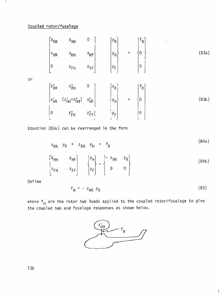
Coupled rotor/fuselage

or

'RR 'RH

'HR 'HH

0 'FH

-z' RR z;H

ziR (ZiH+Zi!jH

0

'HF

'FF

0

0 z:H

> ziAF

z'F'F

Equation (B3a) can be rearranged in the form

'RR YR + 'RH yH = fR

Define

f,, = - Z,,R YR

\ YR

YH' =

YR

YH

YF

- 'HR

=

YR

0 I

where fH are the rotor hub loads applied to the coupled rotor/fuselage to give

(B3a)

(B3b)

@a)

(B4b)

(B5)

the coupled hub and fuselage responses as shown below.

136

BY definition from equation (B4b)

'HF 0-

'FF I _

Solving equation (B7) shows that

'HH = (ZHH - 'HF 'FF 'FH -1 )-1

Thus, equation (B6) becomes

f,, = tZ,,,, - ZHF z;; ZF,,) Y,,

Since z HH 5 Z;IH + ZiH, equation (B9) can be written as

fH = (Z;IH + ZiH - ZiF z:; 1 z;I,,) Y,,

From the definition of mobility for the fuselage alone

Solving equation (Bll) shows that

YiH = (ZiH - ZiF zI;; 1 zpH)-l

and equation (BlO) reduces to

fH = (Z;IH + YLH -'I $.,

(B6)

(B7)

(B8)

(B9)

(BJO)

(B11)

(B12)

(B13)

137

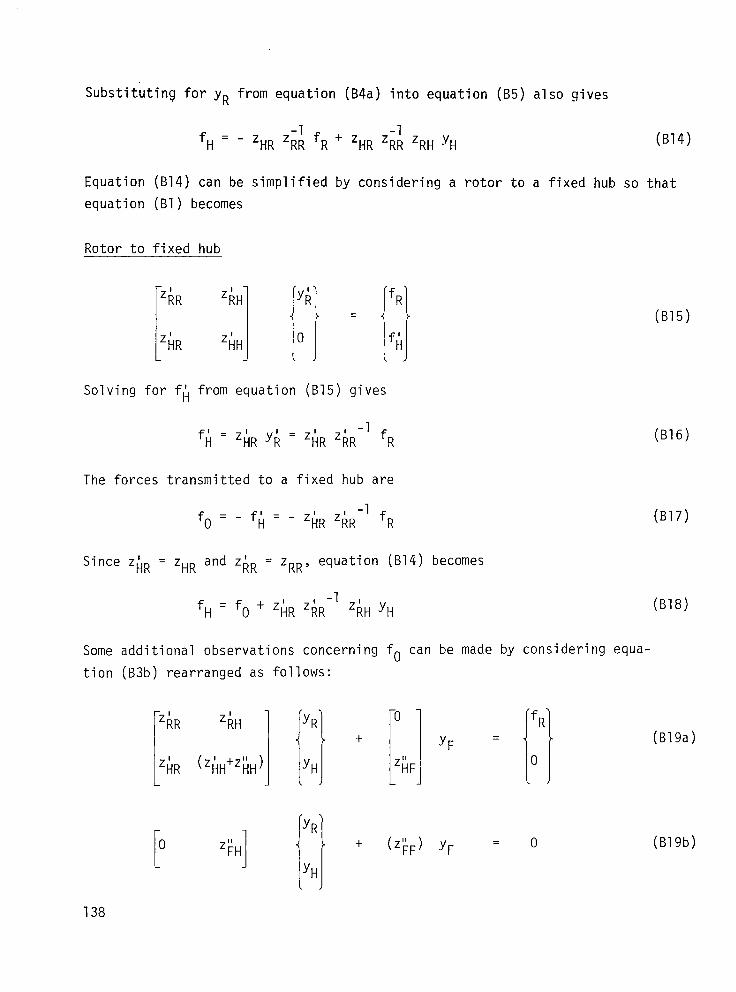
Substituting for yR from equation (B4a) into equation (B5) also gives

fH=-Z HR z;; fR + z -l HR 'RR 'RH yH (B14)

Equation (B14) can be simplified by considering a rotor to a fixed hub so that

equation (Bl) becomes

Rotor to fixed hub

ZRH y ii I II = 0

i

fR

f;l

Solving for f;l from equation (B15) gives

f;l = ZiR yR = Z;IR Z;iR -1 fR

The forces transmitted to a fixed hub are

f. = - f;l = - Z;IR ZRR-l fR

Since z,',~ = zHR and zRR = zRR, equation (B14) becomes

fH = f. + Z;IR ZRR -1 'RH 'H

Some additional observations concerning f. can be made by considering equa-

tion (B3b) rearranged as follows:

(BT5)

(B16)

(B17)

(B18)

(B19a)

(B19b)

138

Substituting for yF from equat ion (B19b) into equation (B19a) 9 i ves

Z;iH yR fR =

1 ZiR (ZIHH + ZiH - z;;F z:; 1 ZPH) I-II I yH 0

Further simplification of equation (820) results in

[(z& - z;IR Z;l; 1 ZiH) + (ZiH - ZiH zp;' ZkH)l yH = - Z;IR

(B20)

z&i ' fR (821)

Equation (B21) can be reduced still further by taking advantage of the mobility

definition for the rotor alone.

ZkR I GH

z;IR z;IH

yRR I yAR

yRH

yAH -I

Solving equation (B22) shows that

YiH = (ZiH - Z;IR Z& 1 Z;IH)- 1

= I 0

0 I

Substituting equations (B12) and (B23) into equation (B21) gives

CY& 1 t Y/11,') yH = - Z;IR Z&l fR

(=‘2)

(~23)

(~24)

and equation (B17) can also be written as

f. = (Y& 1 + y&' ) Y,, (B25)

Substituting equation (825) into equation (B18) and making use of equation (B23)

results in

fH = (ZiH + Y;;i ') Y,, (B26)

139

which is identical to the result derived in equation (B13). Eliminating yR

from equation (Bl) gives

Yi; 1 y;( = - ZiR z& ' fR (B27)

so that

f. = Y& 1 y;( (B28)

Combining equations (B25) and (B28) shows that

or, 1 yH = Y;Ii ' b;, - Y,)

Therefore, fH can be expressed as

where

fH = f. + ZiR z& 1 ZRH yH

fH = f0 + (Z;IH - y&') yH

fH = (Z& + Y& '1 YH

fH = z;(H yH + y;l; ' (Y;, - YH)

-1 fH = 'HH yH

'HH = (';(H + 'HH ,,-I )-1

(B29a)

(B29b)

(B30a)

(B30b)

(B30c)

(B30d)

(B30e)

(B31)

In summary, the rotor hub loads, fH, can be expressed in terms of loads trans-

mitted to a fixed hub and modified by the rotor hub impedances alone, as well

as the coupled rotor/fuselage hub responses.

140

From another point of view equation (B3b) can be written as

Z& YR + z;,, YH = fR (B32a)

Define j,, = - zhR YR - z;IH YH (B33)

where f,, are the rotor hub loads applied to the fuselage alone to give the cou-

pled hub and fuselaqe responses.

Comparing equations (B5) and (B33) shows that

i, = fH - Z;IH yH

Applying equations (B30), fH can be expressed as

i, = f. - Y$ yH (B35a)

n fH = Y$ 1 yH (B35b)

i, = Y&' (Y;, - Y,) (B35c)

Also from equation (B32b)

(B34)

(B36)

141

Equations (B35) and (B36) serve to explain the nature of coupled rotor/fuselage

vibrations with respect to rotor/fuselage dynamic interactions. In particular, the impact of fuselage dynamics on fH and consequently on fuselage vibrations.

Helicopter rotor excitations are very large and one might suspect that hub

responses of a rotor with no fuselage (y,',) may be very large when compared with

hub responses of the coupled rotor/fuselage (y,). In other words,

y;l H " Y

As a consequence of equations (B37) and (B28), equation (B35c) becomes

;H = Y&l y;( = f.

(B37)

(B38)

Therefore, the rotor hub loads acting on a fuselage without the rotor are nearly

independent of the fuselage dynamics. Under this restriction the rotor hub

loads are equal to the forces transmitted to a rigid support. Consider the

extreme case of a fuselage with zero damping which has a natural frequency pre-

cisely at a harmonic of the blade passage frequency. Then yl', = yH since the

fuselage has zero hub impedance (or infinite hub mobility) in this extreme case.

If the undamped fuselage has a natural frequency only slightly removed from the

excitation frequency, then yt; >> yH appears plausible and the conclusion of

equation (838) follows. Also, if with fuselage dynamic changes yH remains

small compared to yi, then there is little change in the transmitted forces as

concluded in equation (B38).

However, the condition that yH is small compared to y;( is a sufficient but not ,. necessary condition for small changes in fH. From equation (B20)

yR II =

yH

zRR

I z;IR

zRH '-1

(ZbH + Y&l, A

fR II 0

(B39)

Consider the case of a fuselage with a natural frequency at the blade passage

frequency for a system without the rotor. In this example YIH is very large

or Yi',;' is very small and equation (B39) indicates that

142

I --

and from equat ion (B35b)

+H = Yi;i 1 yH

YH = Y;1 (B40)

(B47 >

If Y&I does not change appreciably due to fuselage dynamic changes and remains

small, then there is negligible change in yH as equation (839) shows. As a

result there is negligible change in the transmitted rotor loads, fH, given by equation (B41). To illustrate this case, consider an isolated hub-transmission

where

y'rlrH >> Y;F (~42)

and Yi,-,' is very small. For a change in the Fth degree of freedom of the fuse-

lage due to an impedance change nzFF, the changed driving-point hub mobility

is given by

YiF YFH AYhH = YhH - ,

AZFF + YFF

Since Y;H >> Yi',F, it follows that

AYiH = YiH

(B43)

(B44)

and aY&’ remains very small.

Now consider the opposite situation where Y&' is very large or YiH is very

small compared to the z' matrix in equation (B39). This makes yH very small

compared to y;( and the conclusion in equation (B38) follows.

If at blade passage harmonics, equation (B42) does not hold for various

fuselage degrees of freedom, then the fuselage has a major as opposed to local

resonance and the transmitted forces may change considerably due to fuselage

dynamic changes. However, if the fuselage were separated from the rotor, then

143

such a condition could not be tolerated in practice. A major resonance has

modal accelerations relative to points other than the hub which are larger

relative to modal accelerations of other modes. A large modal acceleration

can be looked upon as a small effective mass since

Physically, a small effective mass contributes to the response more signifi-

cantly than a large effective mass for the same loading conditions.

144

---.- _-.-__ -_-_. . .._-_- ._ _..._._ I

REFERENCES

1. Schrage, 0. P.; and Peskar, R. E.: Helicopter Vibration Requirements.

Preprint No. 77.33-33, American Helicopter Society, 33rd Annual National

Forum, May 1977.

2. Veca, Angelo C.: Vibration Effects on Helicopter Reliability and

Maintainability. USAAMRDL TR73-11, April 1973.

3. Berman, A.: A Generalized Coupling Technique for the Dynamic Analysis of

Structural Systems. AIAA/ASME/ASCE/AHS 20th Structures and Materials

.Conference, St. Louis, Missouri, April 1979.

4. Ormiston, R. A.: Comparisons of Several Methods for Predicting Loads on

a Hypothetical Helicopter Rotor. Proceedings of the Meeting of Specialists

on Rotorcraft Dynamics, American Helicopter Society and Ames Research

Center, February 1974.

5. Flannelly, W. G.; Bartlett, F. D., Jr.; and Forsberg, T. D.: Laboratory

Verification of Force Determination, A Potential Tool for Reliability

Testing. USAAMRDL TR76-38, January 1977.

6. Berman, A.; and Flannelly, W. G.: Theory of Incomplete Models. AIAA

Journal, vol. 9, August 1971, pp. 1481-1487.

7. Berman, A.: System Identification of a Complex Structure. AIAA Paper

75-809, Denver, Colorado, May 1975.

8. Chen, J. C.; and Garba, J. A.: Matrix Perturbation for Analytical Model

Improvement. AIAA Paper 79-0831, St. Louis, Missouri, April 1979.

9. Kennedy, C. C.; and Pancu, C. D. P.: Use of Vectors in Vibration Measure-

ment and Analysis. Journal Aeronautical Sciences, vol. 14, no. 11,

November 1947.

145

10. Klosterman, A. L .; and Lemon, J. R.: Dynamic Analysis via the Building

Block Approach. Shock and Vibration Bulletin, 42 (4), 97-104,

January 1972.

11. Ewins, D. J.: Whys and Wherefores of Modal Testing. SEE Journal,

September 1979.

146

1. Report No. 2. Government Accession No. 3. Recipient’s Catalog No.

NASA CR-3429 4. Title and Subtitle

ANALYTICAL TESTING

I 5. Report Date

May 1981 6. Performing Organization Code

7. Author(s)

W. G. Flannelly, J. A. Fabunmi, and E. J. Nagy

9. Performing Organization Name and Address

Kaman Aerospace Corporation Old Windsor Road Bloomfield, Connecticut 06002

12. Sponsoring Agency Name and Address

8. Performing Orgamzation Report No.

R-1614 10. Work Unit No.

11. Contract or Grant No.

NASl-15414 13. Type of Report and Period Covered

Contractor Report 6127178 - 9115180

National Aeronautics and Space Administration Washington, DC 20546

14. Sponsoring Agency Code

15. SuPPlementarV Notes Langley Technical Monitor: F. D. Bartlett, Jr. The Contract research effort which has led to the results in this report was financially supported by the Structures Laboratory, AVRADCOM Research and Technology Laboratories. Final Report

6. Abstract

Analytical methods for combining flight acceleration and strain data with shake test mobility data to predict the effects of structural changes on flight vibrations and strains are presented. This integration of structural dynamic analysis with flight performance is referred to as analytical testing. The objective of this methodology is to analytically estimate the results of flight testing contemplated structural changes with minimum flying and change trials. The category of changes to the aircraft includes mass, stiffness, absorbers, isolators, and active suppressors. Examples of applying the analytical testing methodology using flight test and shake test data measured on an AH-1G helicopter are included. The techniques and procedure for vibration testing and modal analysis are also described.

7. Key Words (Suggested by Author(s))

Structural dynamics Modal analysis Flight testing Stress analysis Shake testing Helicopters Vibrations Suppressors Absorbers Isolators

16. Distribution Statement

Unclassified - Unlimited

Subject Category 39

9. Security Classif. (of this report1 20. Security Classif. (of this page) 21. No. of Pages 22. Price

Unclassified Unclassified 152 A08

For sale by the National Technrcal Information Service, Sprrnefreld, Vrrgrnra 22161

NASA-Lang1 ey , 1981