The use of acousto-ultrasonic techniques to measure ... · PDF fileThe use of acousto-ultrasonic techniques to measure propagation time through glass-fibre reinforced coupons T TG

`

The use of acousto-ultrasonic techniques to measure propagation time through glass-fibre reinforced

coupons

OB_TG5_R010 rev. 000

Version 1

Confidential

TG 5

Alan Ruddell Geoff Dutton

(CCLRC-RAL)

OPTIMAT BLADES

OB_TG5_R00x_000 OPTIMAT BLADES Page 2 of 32

Last saved: 02/03/2006 17:15

Change record

Issue/revision date pages Summary of changes Version 1 21-02-06 30 Initial draft


Last saved: 02/03/2006 17:15

Contents

1. INTRODUCTION....................................................................................................................................4

2. METHODOLOGY...................................................................................................................................6 2.1. THEORETICAL BASIS ...........................................................................................................................6 2.2. ILLUSTRATION OF CHIRP PULSE COMPRESSION ..................................................................................7 2.3. PRACTICAL CHIRP PULSE AND TRANSDUCER BANDWIDTH.................................................................9

3. EXPERIMENTAL PROCEDURE .......................................................................................................14

4. RESULTS................................................................................................................................................15 4.1. DIRECTLY COUPLED SENSORS ..........................................................................................................15 4.2. COUPON MEASUREMENTS.................................................................................................................15 4.3. FLAT PLATE MEASUREMENTS...........................................................................................................17

5. CONCLUSIONS.....................................................................................................................................18

6. BIBLIOGRAPHY ..................................................................................................................................19

7. APPENDICES ........................................................................................................................................21 7.1. APPENDIX 1: EXPERIMENTAL SET-UP...............................................................................................21 7.2. APPENDIX 2: SPECIFICATION OF THE PAC PICO SENSORS ...............................................................24 7.3. APPENDIX 3: CONFIGURATION OF SENSORS, PRE-AMPS, AND AEDSP-32/16..................................25 7.4. APPENDIX 4: USING MI-TRA MISTRAS TRANSIENT RECORDER .....................................................27 7.5. APPENDIX 5: EXPERIMENTAL DATA FILES........................................................................................29


Last saved: 02/03/2006 17:15

1. Introduction

The objective of this work was to measure the time-of-flight of ultrasonic signals through glass-fibre coupons before and after fatigue testing, to assess whether this could be a useful method to determine material condition. During Phase 1 of the main OPTIMAT BLADES testing program, Philippidis et al (2005) at the University of Patras conducted tests to measure the residual strength of various coupons after fatigue testing. Several other tests were conducted, including initial acousto-ultrasonic tests, using two PAC1 Pico sensors to transmit and receive a sinusoidal signal with frequency sweep from 10 to 2000 kHz. The time-series of transmitted and received signals were plotted and compared. Two types of coupons were tested, Standard unidirectional coupons @90°, and standard ISO ±45º coupons. The reports by Philippidis et al. concluded that there was generally no correlation of residual strength with the results of acousto-ultrasonic tests, although one test did indicate a time lag between signals measured before and after fatigue. Acousto-ultrasonic testing is now used in a range of non-destructive examination (NDE) applications, and uses a wide range of transducer technology and specifications. A short review of the technical literature has been conducted, covering a range of complex issues, including signal types and processing methods, and transducers. A short ultrasonic pulse, ideally a Dirac delta pulse, would provide a means of measuring time-of-flight, provided that a transducer with high bandwidth was available, and high power was possible, in order to achieve a usable signal to noise ratio. Practical transducers used for signal transmission and reception have limited bandwidth and power, and the resulting envelope of the band-limited received pulse makes accurate measurement of time-delay difficult. An alternative approach is use a longer ultrasonic pulse, together with signal processing to compress the received signal into a short pulse, to give good resolution in the time domain. The use of chirp frequency (sweep frequency) transmission is used by bats (Dryer, 2004) and is a well established method in radar systems. The technique has been recently applied to ultrasonic testing. The use of linear frequency-modulated pulses in ultrasonic testing has tended to follow the techniques successfully used in radar, even though the systems are quite different. In a radar system, the transmitting and receiving antenna and amplifiers, and the transmission medium, can have a wide bandwidth and a constant amplitude transfer function. The situation in an ultrasonics testing system is quite different, where the tranducers and transmission may be band-limited, causing a spectral mismatch with the excitation at constant amplitude versus frequency, and a reduction in overall efficiency. Pollakowski (1994) describes this problem, and suggests the use of a chirp signal excitation with amplitude matched to the system transfer function (i.e. the transducer transfer function), which can result in increased amplitude of the compressed pulse.

1 Physical Acoustics Corporation http://www.pacndt.com/

http://www.pacndt.com/


Last saved: 02/03/2006 17:15

Air-coupled ultrasound is used to measure the characteristics of materials without contact, where conventional methods such as water coupling are not suitable. Buckley (2000) described the measures used to compensate for the high path loss, in order to achieve an acceptable signal to noise ratio (SNR). The usual approach is to use a sinusoidal tone-burst, however this has the disadvantage that accurate measurement of timing is difficult, although good results can be obtained in through transmission applications where only amplitude is measured. Gan (2003) described the use of a broad-band capacitive transducer system with chirp signal and pulse compression processing to measure features of paper products such as bank notes, high-quality paper, stamps, and sealed joints. The work concentrated on amplitude images, although velocity (time-of-flight) can also be measured. Gan (2004 and 2005) also described the use of swept frequency multiplication (SFM), derived in part from an analogous method used in optics known as optical frequency domain reflectometry (OFDR). Instead of cross-correlating the received signal with a reference chirp, the SFM system simply multiplies the received signal with a reference chirp at a fixed time delay. The chief advantage of the method is that if offers the possibility of reduced signal processing times, which could be important in high-resolution imaging of material properties. Gan (2005) concluded that the two techniques are comparable in their ability to improve the SNR. Measurement of time-of-flight is used in ultrasonic flow metering. Folkestad (1993) describes chirp excitation, and a mixture of continuous wave and chirp signals, followed by pulse compression techniques, and concludes that the selection of a proper transducer, and the type and duration of signals are important. Dooley (1995) suggests an alternative method to that described by Folkestad, and shows how the correct cycle of a delayed tone-burst can be identified by varying the tone-burst frequency. Several of the mentioned papers emphasise the importance of choosing a transducer and signal characteristics appropriate for the application. Piezo transducers are essentially resonant devices, and although construction techniques can be used to introduce suitable damping, the bandwidth tends to be relatively narrow. Capacitive transducers can provide wide bandwidth in air-coupled applications and give superior performance. The latest technique used in fabricating capacitive transducers is MEMS (micro-electro-mechanical systems) technology, as described by Cittadine (2000). A laser interferometer can be used as the receiver sensor, with the advantage of non-contact operation. However the nature of light scattering on ordinary surfaces means that the received sensitivity is low in most practical applications. Koehler (1997) describes how the SNR in ultrasonic testing of concrete can be improved by optical scanning and making measurements when the interference speckles are brightest.


Last saved: 02/03/2006 17:15

2. Methodology

2.1. Theoretical basis The first step is to transmit and receive a signal transmitted through a coupon, subject to attenuation and added noise. The method used follows from that first developed in 1950 for radar, using a long duration signal of low peak power, and using pulse compression at the receiver to obtain a narrow pulse. The concept can be achieved by using a linearly frequency-modulated signal known as a chirp pulse, and using matched filtering or cross-correlation at the receiver to achieve a narrow pulse with good SNR. In the present application, the narrow pulse would provide a means of measuring the time delay (time-of-flight) of the transmitted signal through the coupon, which may indicate the condition of the material. The modulated chirp signal is given by:

( ) ( ) ⎟⎠⎞

⎜⎝⎛ += 2

1sin. tTBttAts πω for (1) Tt ≤≤0

where A(t) is the amplitude modulation of the chirp pulse, ω1 is the start frequency, ω2 is the end frequency, B is the bandwidth (ω2 – ω1), and T is the pulse duration. A linear frequency-modulation during the pulse duration is assumed. Amplitude windows can be applied to reduce the amount of time-domain side-lobes in the signal. The amplitude modulation A(t) can be various waveforms, for example: constant amplitude: for (2) ( ) 1=tA Tt ≤≤0

Hanning function: ( ) ⎥⎦

⎤⎢⎣

⎡⎟⎠⎞

⎜⎝⎛−=

TttA π2cos1 for (3) Tt ≤≤0

Taylor weighting: ( ) ⎥⎦

⎤⎢⎣

⎡⎟⎠⎞

⎜⎝⎛−=

TttA π2cos84.01

84.11 for (4) Tt ≤≤0

Applying a matched filter to the received signal is analogous to performing a cross-correlation between the reference (transmitted) signal and the received signal. The matched filter for a transmitted signal s(t) will in general have an impulse response h(t) given by: ( ) ( )ttsAth ff −= (5) where the constants Af and tf are amplitude and time delay constants imposed by the matched filter. The received signal is in general given by: ( ) ( )ddr ttsAts −= (6)


Last saved: 02/03/2006 17:15

where the constants Ad and td are amplitude and time delay constants imposed by the transmission. The output of the matched filter is given by the convolution of the input signal to the filter, and the impulse response of the matched filter.

(7) ( ) ( ) ( )∫∞+

∞−

−= τττ dthsts ro .

(8) ( ) ( ) ( )∫∞+

∞−

+−−= τττ dttstsAAts fdfd .0

Assuming that the received signal is exactly equal to the transmitted signal (Af = 1 and td = 0) and the matched filter amplitude Af = 1 and time delay td = 0, then the matched filter output is given by Eqn 9, and is the autocorrelation function of the signal s(t).

(9) ( ) ( ) ( )∫∞+

∞−

−= τττ dtsstso .

The maximum value of the autocorrelation function is at time t = 0, and is proportional to the total energy in the transmitted signal, obtained with a short duration, high power signal, or a long duration low power signal:

(10) ( ) ( )∫∞+

∞−

= ττ dsso .0 2

In practice the received signal is subject to amplitude and time delay constants, and the matched filter output is given by:

(11) ( ) ( ) ( )∫∞+

∞−

−−= τττ dtstsAts ddo .

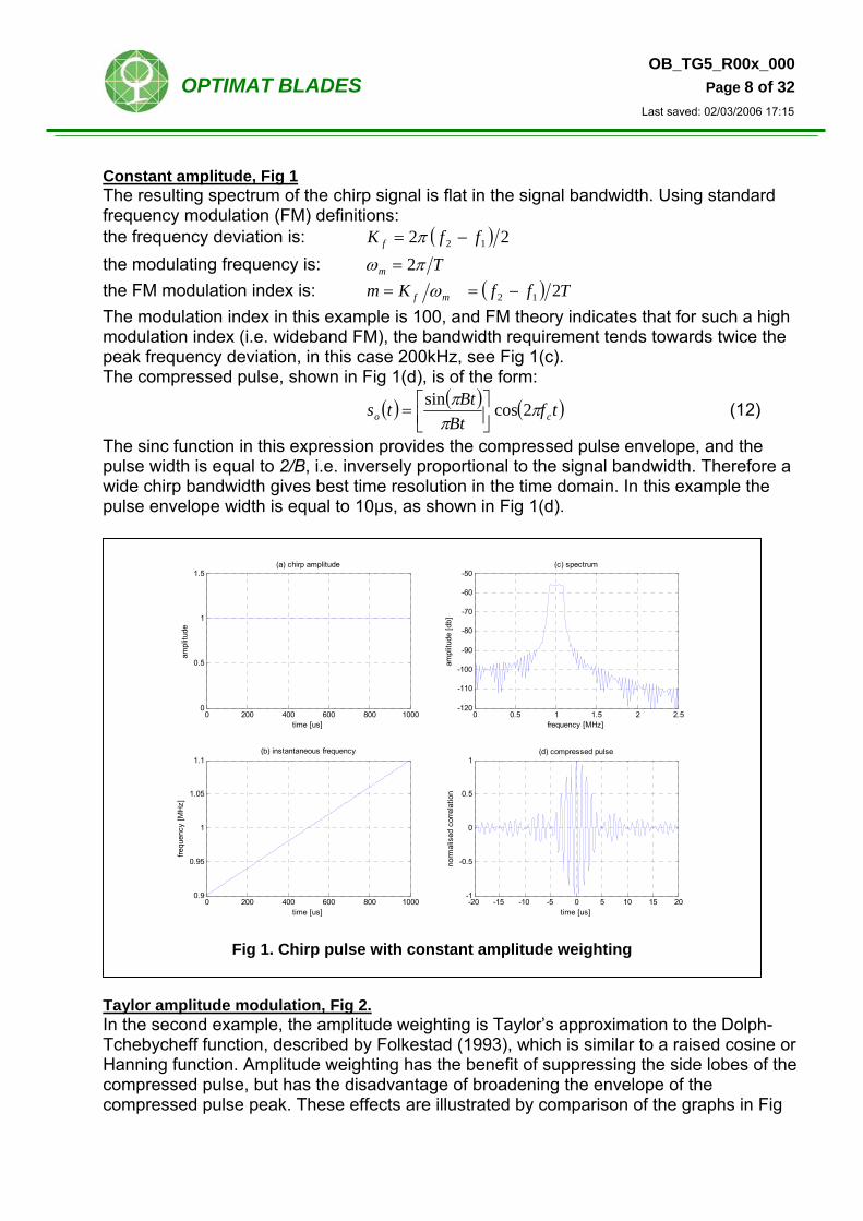
The maximum of the matched filter output is at time t = td and indicates the transmission time-of-flight. 2.2. Illustration of chirp pulse compression The following parameters were chosen to illustrate the method: chirp start frequency f1 = 900 kHz (where ω1 = 2πf1) chirp end frequency f2 = 1100 kHz (where ω2 = 2πf2) bandwidth B = (f2 – f1) = 200 kHz pulse duration T = 1 ms Two cases for the amplitude modulation A(t) are illustrated in Fig 1 (constant amplitude) and Fig 2 (Taylor weighting). In each case four graphs are presented; (a) the amplitude modulation, (b) the instantaneous frequency (linear frequency modulation), (c) the spectrum of the chirp signal, and (d) the compressed pulse produced by cross-correlation.


Last saved: 02/03/2006 17:15

Constant amplitude, Fig 1 The resulting spectrum of the chirp signal is flat in the signal bandwidth. Using standard frequency modulation (FM) definitions: the frequency deviation is: ( ) 22 12 ffK f −= π the modulating frequency is: Tm πω 2= the FM modulation index is: ( ) TffKm mf 212 −== ω The modulation index in this example is 100, and FM theory indicates that for such a high modulation index (i.e. wideband FM), the bandwidth requirement tends towards twice the peak frequency deviation, in this case 200kHz, see Fig 1(c). The compressed pulse, shown in Fig 1(d), is of the form:

( ) ( ) ( tfBt

Btts co πππ 2cossin

⎥⎦⎤

⎢⎣⎡= ) (12)

The sinc function in this expression provides the compressed pulse envelope, and the pulse width is equal to 2/B, i.e. inversely proportional to the signal bandwidth. Therefore a wide chirp bandwidth gives best time resolution in the time domain. In this example the pulse envelope width is equal to 10µs, as shown in Fig 1(d).

0 200 400 600 800 10000

0.5

1

1.5

ampl

itude

time [us]

(a) chirp amplitude

0 0.5 1 1.5 2 2.5-120

-110

-100

-90

-80

-70

-60

-50

ampl

itude

[db]

frequency [MHz]

(c) spectrum

0 200 400 600 800 10000.9

0.95

1

1.05

1.1

frequ

ency

[MH

z]

time [us]

(b) instantaneous frequency

-20 -15 -10 -5 0 5 10 15 20-1

-0.5

0

0.5

1

norm

alis

ed c

orre

latio

n

time [us]

(d) compressed pulse

Fig 1. Chirp pulse with constant amplitude weighting

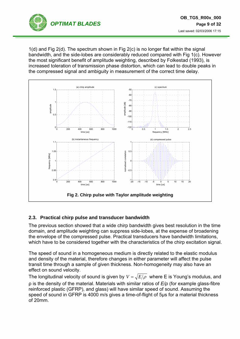
Taylor amplitude modulation, Fig 2. In the second example, the amplitude weighting is Taylor’s approximation to the Dolph-Tchebycheff function, described by Folkestad (1993), which is similar to a raised cosine or Hanning function. Amplitude weighting has the benefit of suppressing the side lobes of the compressed pulse, but has the disadvantage of broadening the envelope of the compressed pulse peak. These effects are illustrated by comparison of the graphs in Fig


Last saved: 02/03/2006 17:15

1(d) and Fig 2(d). The spectrum shown in Fig 2(c) is no longer flat within the signal bandwidth, and the side-lobes are considerably reduced compared with Fig 1(c). However the most significant benefit of amplitude weighting, described by Folkestad (1993), is increased toleration of transmission phase distortion, which can lead to double peaks in the compressed signal and ambiguity in measurement of the correct time delay.

0 200 400 600 800 10000

0.5

1

1.5

ampl

itude

time [us]

(a) chirp amplitude

0 0.5 1 1.5 2 2.5-120

-110

-100

-90

-80

-70

-60

-50

ampl

itude

[db]

frequency [MHz]

(c) spectrum

0 200 400 600 800 10000.9

0.95

1

1.05

1.1

frequ

ency

[MH

z]

time [us]


-20 -15 -10 -5 0 5 10 15 20-1

-0.5

0

0.5

1

norm

alis

ed c

orre

latio

n

time [us]


Fig 2. Chirp pulse with Taylor amplitude weighting

2.3. Practical chirp pulse and transducer bandwidth The previous section showed that a wide chirp bandwidth gives best resolution in the time domain, and amplitude weighting can suppress side-lobes, at the expense of broadening the envelope of the compressed pulse. Practical transducers have bandwidth limitations, which have to be considered together with the characteristics of the chirp excitation signal. The speed of sound in a homogeneous medium is directly related to the elastic modulus and density of the material, therefore changes in either parameter will affect the pulse transit time through a sample of given thickness. Non-homogeneity may also have an effect on sound velocity. The longitudinal velocity of sound is given by ρEV = where E is Young’s modulus, and ρ is the density of the material. Materials with similar ratios of E/ρ (for example glass-fibre reinforced plastic (GFRP), and glass) will have similar speed of sound. Assuming the speed of sound in GFRP is 4000 m/s gives a time-of-flight of 5µs for a material thickness of 20mm.


Last saved: 02/03/2006 17:15

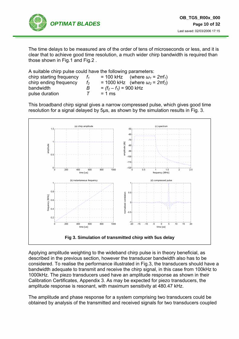
The time delays to be measured are of the order of tens of microseconds or less, and it is clear that to achieve good time resolution, a much wider chirp bandwidth is required than those shown in Fig.1 and Fig.2 . A suitable chirp pulse could have the following parameters: chirp starting frequency f1 = 100 kHz (where ω1 = 2πf1) chirp ending frequency f2 = 1000 kHz (where ω2 = 2πf2) bandwidth B = (f2 – f1) = 900 kHz pulse duration T = 1 ms This broadband chirp signal gives a narrow compressed pulse, which gives good time resolution for a signal delayed by 5µs, as shown by the simulation results in Fig. 3.

0 200 400 600 800 10000

0.5

1

1.5

ampl

itude

time [us]

(a) chirp amplitude

0 0.5 1 1.5 2 2.5-120

-110

-100

-90

-80

-70

-60

-50

ampl

itude

[db]

frequency [MHz]

(c) spectrum

0 200 400 600 800 1000

0.2

0.4

0.6

0.8

1

frequ

ency

[MH

z]

time [us]


-20 -15 -10 -5 0 5 10 15 20-1

-0.5

0

0.5

1

norm

alis

ed c

orre

latio

n

time [us]


Fig 3. Simulation of transmitted chirp with 5us delay

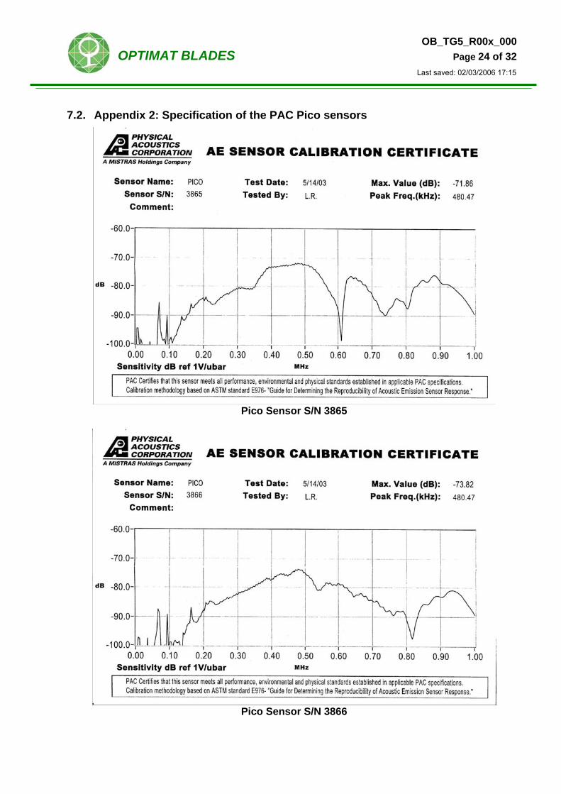
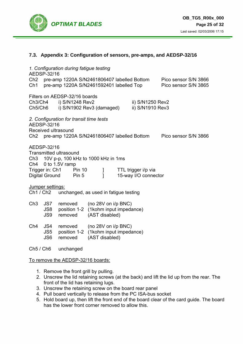
Applying amplitude weighting to the wideband chirp pulse is in theory beneficial, as described in the previous section, however the transducer bandwidth also has to be considered. To realise the performance illustrated in Fig.3, the transducers should have a bandwidth adequate to transmit and receive the chirp signal, in this case from 100kHz to 1000kHz. The piezo transducers used have an amplitude response as shown in their Calibration Certificates, Appendix 3. As may be expected for piezo transducers, the amplitude response is resonant, with maximum sensitivity at 480.47 kHz. The amplitude and phase response for a system comprising two transducers could be obtained by analysis of the transmitted and received signals for two transducers coupled


Last saved: 02/03/2006 17:15

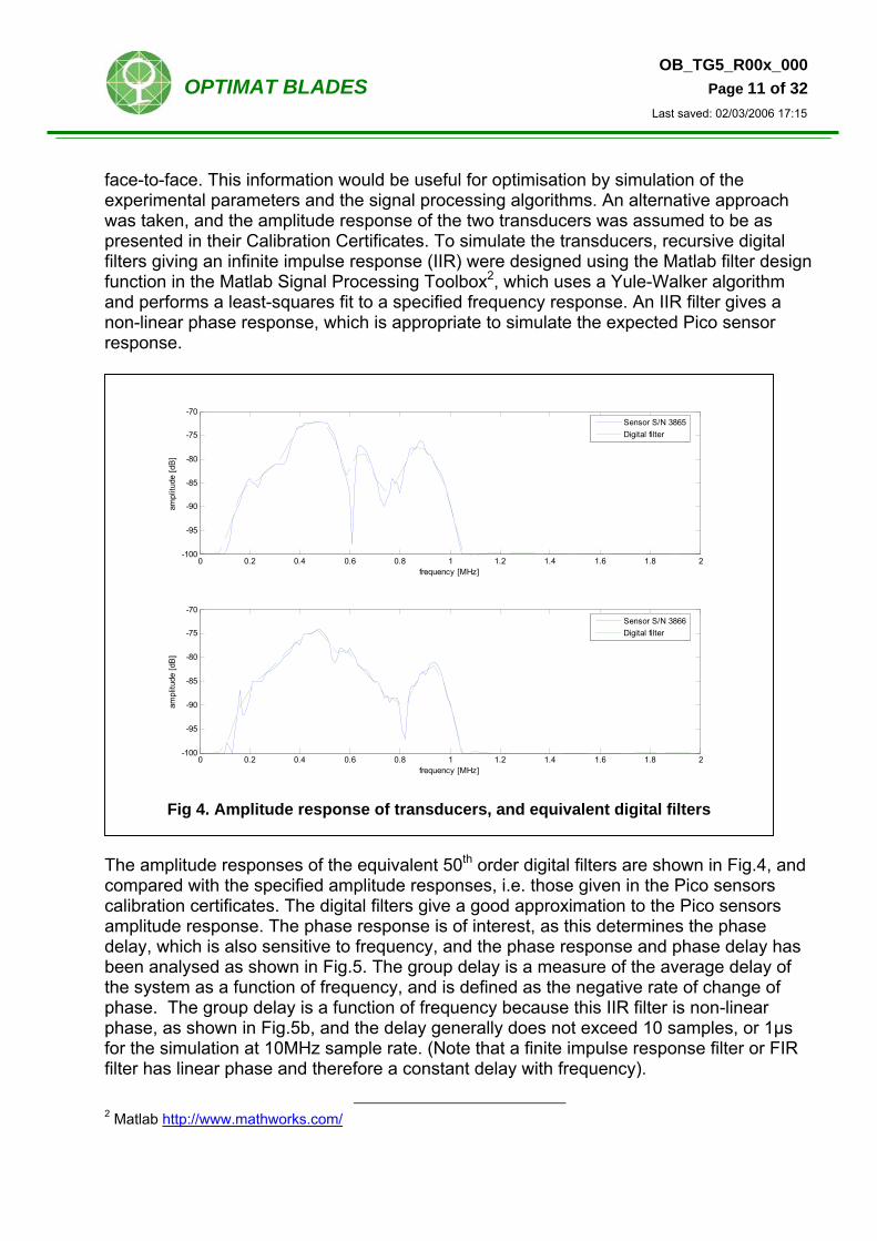
face-to-face. This information would be useful for optimisation by simulation of the experimental parameters and the signal processing algorithms. An alternative approach was taken, and the amplitude response of the two transducers was assumed to be as presented in their Calibration Certificates. To simulate the transducers, recursive digital filters giving an infinite impulse response (IIR) were designed using the Matlab filter design function in the Matlab Signal Processing Toolbox2, which uses a Yule-Walker algorithm and performs a least-squares fit to a specified frequency response. An IIR filter gives a non-linear phase response, which is appropriate to simulate the expected Pico sensor response.

The amplitude responses of the equivalent 50th order digital filters are shown in Fig.4, and compared with the specified amplitude responses, i.e. those given in the Pico sensors calibration certificates. The digital filters give a good approximation to the Pico sensors amplitude response. The phase response is of interest, as this determines the phase delay, which is also sensitive to frequency, and the phase response and phase delay has been analysed as shown in Fig.5. The group delay is a measure of the average delay of the system as a function of frequency, and is defined as the negative rate of change of phase. The group delay is a function of frequency because this IIR filter is non-linear phase, as shown in Fig.5b, and the delay generally does not exceed 10 samples, or 1µs for the simulation at 10MHz sample rate. (Note that a finite impulse response filter or FIR filter has linear phase and therefore a constant delay with frequency).

2 Matlab http://www.mathworks.com/

0 0.2 0.4 0.6 0.8 1 1.2 1.4 1.6 1.8 2-100

-95

-90

-85

-80

-75

-70

frequency [MHz]

ampl

itude

[dB

]

Sensor S/N 3865Digital filter

0 0.2 0.4 0.6 0.8 1 1.2 1.4 1.6 1.8 2-100

-95

-90

-85

-80

-75

-70

frequency [MHz]

ampl

itude

[dB

]

Sensor S/N 3866Digital filter

Fig 4. Amplitude response of transducers, and equivalent digital filters

http://www.mathworks.com/


Last saved: 02/03/2006 17:15

0 0.5 1 1.5 2-3

-2

-1

0

1

2

3

Frequency (MHz)

Pha

se (r

adia

ns)

Phase Response

0 0.5 1 1.5 2-50

0

50

Frequency (MHz)

Gro

up d

elay

(in

sam

ples

)

Group Delay

Fig 5. Phase and group delay response of digital filter (SN3866)

The broadband chirp signal (100kHz to 1MHz), with a 5µs delay, was passed through the two digital filters, to simulate the response of the proposed system. The results are shown in Fig.6, and show that the envelope of the received waveform is bandlimited by the filters, as expected.

0 0.2 0.4 0.6 0.8 1-0.6

-0.4

-0.2

0

0.2

0.4

0.6

ampl

itude

time [ms]

(a) received chirp waveform

0 0.5 1 1.5 2 2.5-120

-110

-100

-90

-80

-70

-60

-50

ampl

itude

[db]

frequency [MHz]

(c) spectrum

0 0.2 0.4 0.6 0.8 1

0.2

0.4

0.6

0.8

1

frequ

ency

[MH

z]

time [ms]


-20 -15 -10 -5 0 5 10 15 20-1

-0.5

0

0.5

1

norm

alis

ed c

orre

latio

n

time [us]


Fig 6. Simulation of transmitted chirp using Pico sensors, and 5us delay

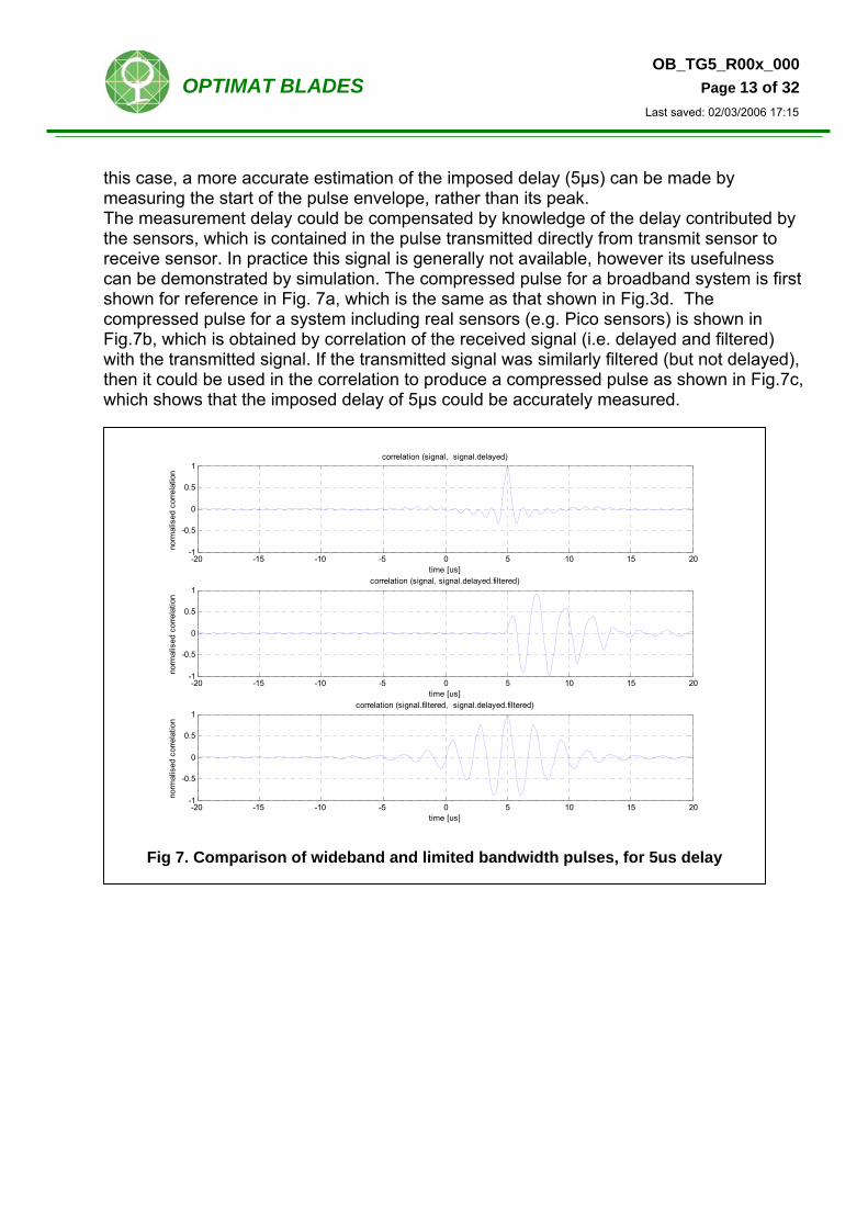
The compressed pulse shows an overall delay of around 7µs to 8µs, which is consistent with the imposed delay of 5µs and the group delay of two filters in series. However the width of the compressed pulse for the bandlimited system (compare with Fig.3 for a wideband pulse) makes accurate determination of the delay difficult. It is suggested that in


Last saved: 02/03/2006 17:15

this case, a more accurate estimation of the imposed delay (5µs) can be made by measuring the start of the pulse envelope, rather than its peak. The measurement delay could be compensated by knowledge of the delay contributed by the sensors, which is contained in the pulse transmitted directly from transmit sensor to receive sensor. In practice this signal is generally not available, however its usefulness can be demonstrated by simulation. The compressed pulse for a broadband system is first shown for reference in Fig. 7a, which is the same as that shown in Fig.3d. The compressed pulse for a system including real sensors (e.g. Pico sensors) is shown in Fig.7b, which is obtained by correlation of the received signal (i.e. delayed and filtered) with the transmitted signal. If the transmitted signal was similarly filtered (but not delayed), then it could be used in the correlation to produce a compressed pulse as shown in Fig.7c, which shows that the imposed delay of 5µs could be accurately measured.

-20 -15 -10 -5 0 5 10 15 20-1

-0.5

0

0.5

1

norm

alis

ed c

orre

latio

n

time [us]

correlation (signal, signal.delayed)

-20 -15 -10 -5 0 5 10 15 20-1

-0.5

0

0.5

1

norm

alis

ed c

orre

latio

n

time [us]

correlation (signal, signal.delayed.filtered)

-20 -15 -10 -5 0 5 10 15 20-1

-0.5

0

0.5

1

norm

alis

ed c

orre

latio

n

time [us]

correlation (signal.filtered, signal.delayed.filtered)

Fig 7. Comparison of wideband and limited bandwidth pulses, for 5us delay


Last saved: 02/03/2006 17:15

3. Experimental procedure

The experimental system used the equipment specified in Appendix 1, and included: - A function generator to repeatedly trigger a chirp signal - A ramp generator to define the linear frequency ramp - A sine-wave generator with frequency control to produce the chirp signal - Transmit and receive sensors (Pico sensors) - A data acquisition system with pre-amplifier for the received signal (Mistras) The chirp pulse was a sinusoidal signal with frequency sweep from 100kHz to 1MHz in 1ms, with amplitude 4V p-p. The repetition rate was around 300Hz. This signal was applied to a Pico sensor, mounted on the sample under investigation, and the signal transmitted through the sample was received by a second Pico sensor. A pre-amplifier set to 40dB was used to interface to the Mistras system. The Mistras system was set up as detailed in Appendix 5, and was triggered by a single manual trigger via the ramp generator board, and used to record the transmitted and received signals. Operation of the Mistras system is described in Appendix 4. The Pico sensors were placed in contact with the sample using ultrasonic couplant (Sonotrace or Ultragel, by Diagnostic Sonar), and held in position using elastic bands. The experiments conducted and associated conditions are listed in Appendix 6, and include: - Direct coupling of the sensors - Measurements on coupons before and after fatigue damage - Measurements on a flat plate, with and without flaws


Last saved: 02/03/2006 17:15

4. Results

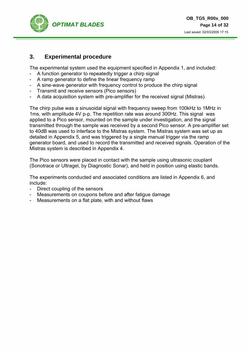
Measurements of transmission delay were made to the start of the compressed pulse envelope, as described in Section 2.3. 4.1. Directly coupled sensors The sensors were directly coupled face-to-face. The measured delay (to the start of the pulse envelope) was around 1µs, as shown in Fig 8. This is nearly in agreement with the simulation results described in Section 2.3, which showed 0µs to the start of the envelope. This reason for this small delay has not been discovered, however the result shows that 1µs should be subtracted from all delay measurements.

0 0.1 0.2 0.3 0.4 0.5 0.6 0.7 0.8 0.9 1-10

-5

0

5

10

volts

time [ms]

AU050916 DCOUP2: received signal, 0 to 1 ms

-20 -15 -10 -5 0 5 10 15 20-1

-0.5

0

0.5

1

norm

alis

ed c

orre

latio

n

time [us]

AU050916 DCOUP2: i/p-o/p cross-correlation (for time 0 to 1 ms)

Fig 8. Sensors directly coupled face-to-face

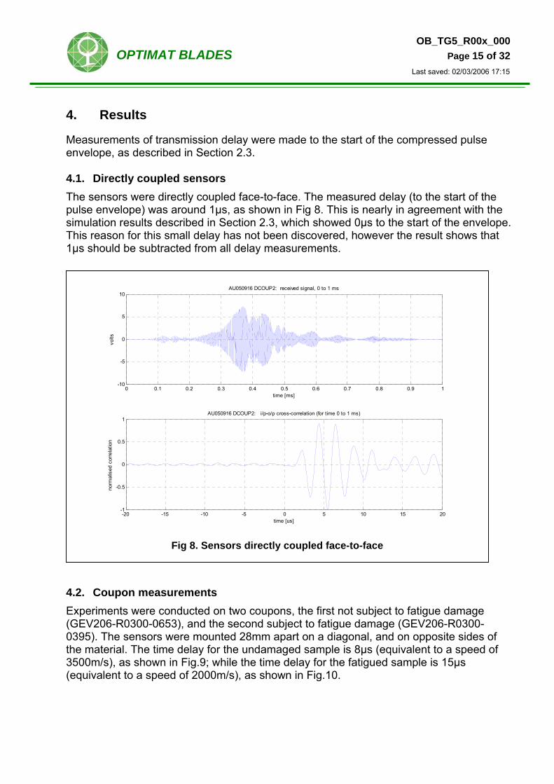
4.2. Coupon measurements Experiments were conducted on two coupons, the first not subject to fatigue damage (GEV206-R0300-0653), and the second subject to fatigue damage (GEV206-R0300-0395). The sensors were mounted 28mm apart on a diagonal, and on opposite sides of the material. The time delay for the undamaged sample is 8µs (equivalent to a speed of 3500m/s), as shown in Fig.9; while the time delay for the fatigued sample is 15µs (equivalent to a speed of 2000m/s), as shown in Fig.10.


Last saved: 02/03/2006 17:15

0 0.1 0.2 0.3 0.4 0.5 0.6 0.7 0.8 0.9 1-0.5

0

0.5

volts

time [ms]

AU050909 U653BF5: received signal, 0 to 1 ms

-50 -40 -30 -20 -10 0 10 20 30 40 50-1

-0.5

0

0.5

1

norm

alis

ed c

orre

latio

n

time [us]

AU050909 U653BF5: i/p-o/p cross-correlation (for time 0 to 1 ms)

Fig 9. Sensors 28mm apart on sample GEV206-R0300-0653 (no fatigue)

0 0.1 0.2 0.3 0.4 0.5 0.6 0.7 0.8 0.9 1-0.04

-0.02

0

0.02

0.04

volts

time [ms]

AU050909 U395PF12: received signal, 0 to 1 ms

-50 -40 -30 -20 -10 0 10 20 30 40 50-1

-0.5

0

0.5

1

norm

alis

ed c

orre

latio

n

time [us]

AU050909 U395PF12: i/p-o/p cross-correlation (for time 0 to 1 ms)

Fig 10. Sensors 28mm apart on sample GEV206-R0300-0395 (after fatigue failure)


Last saved: 02/03/2006 17:15

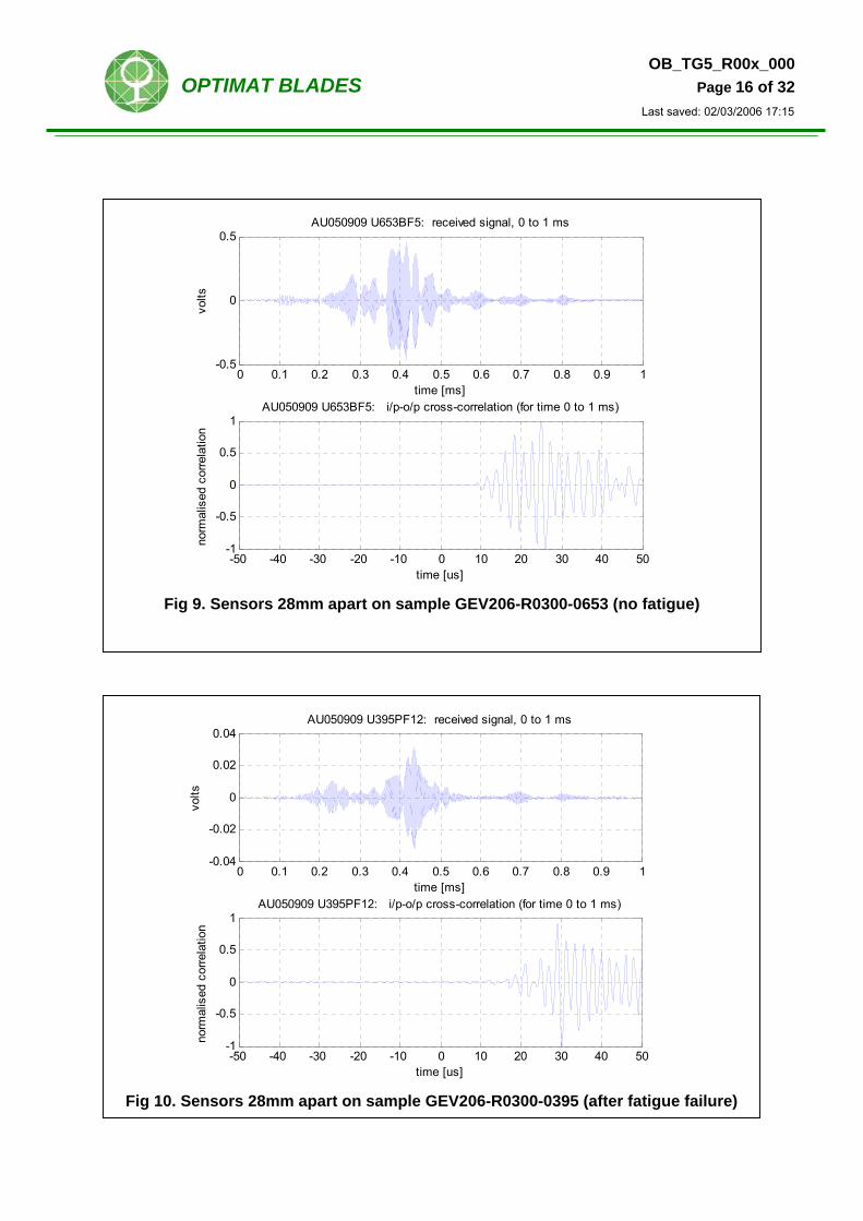
4.3. Flat plate measurements Tests were conducted for sensor spacings of 30, 60, 120, and 151mm on a flat plate of a different glass/polyester material without flaws. An example of the analysis for sensor spacing of 30mm is shown in Fig. 11. The delays for the various sensor spacings, as shown in Table 1, were all consistent with a speed of around 3300m/s.

0 0.1 0.2 0.3 0.4 0.5 0.6 0.7 0.8 0.9 1-2

-1

0

1

2

volts

time [ms]

AU051010 NF2D0302: received signal, 0 to 1 ms

-50 -40 -30 -20 -10 0 10 20 30 40 50-1

-0.5

0

0.5

1

norm

alis

ed c

orre

latio

n

time [us]

AU051010 NF2D0302: i/p-o/p cross-correlation (for time 0 to 1 ms)

Fig.11. Sensors 30mm apart on flat plate NF2..

Sensor spacing [mm]

Delay (time of flight [µs]

30 9 60 19 90 27

120 35 151 45

Table 1. Delays for various sensor spacings


Last saved: 02/03/2006 17:15

Tests were also conducted for a sensor spacing of 60mm on a flat plate of similar material containing 20mm square PTFE flaws 1mm, 2.5mm, 4mm, and 5mm deep. The results were consistent, with a delay of 19µs for all tests, which is the same as that measured for the plate with no flaws. An example for the 5mm deep flaw is shown in Fig.12.

0 0.1 0.2 0.3 0.4 0.5 0.6 0.7 0.8 0.9 1-0.5

0

0.5

volts

time [ms]

AU051010 E33F52: received signal, 0 to 1 ms

-100 -80 -60 -40 -20 0 20 40 60 80 100-1

-0.5

0

0.5

1

norm

alis

ed c

orre

latio

n

time [us]

AU051010 E33F52: i/p-o/p cross-correlation (for time 0 to 1 ms)

Fig.12. Sensors 60mm apart on flat plate E33 with a 5mm deep flaw

5. Conclusions

Piezo transducers were used to obtain the results presented in this report. Although some correlation of the time-of-flight measurements with material condition was observed, the resolution of time measurements was subject to ambiguity. Furthermore the coupling of the sensors to the material was observed to be critical and appeared to affect the amplitude of the received waveform. No attempt was made to explain this or to quantify the effect. However it was found that the time-of-flight measurement could still be made despite the variation in coupling. It is recommended that future work should wide bandwidth transducers, for example capacitive transducers, preferably water or air-coupled. This would enable experiments to be conducted using a wider bandwidth and giving better resolution in the measurement of time-of-flight.


Last saved: 02/03/2006 17:15

6. Bibliography

Buckley J., Air-coupled ultrasound – A millennial review, Proc. 15th World Conference on Nondestructive Testing, Rome, 15-21 October 2000. Available from: http://www.ndt.net/article/wcndt00/index.htm Cittadine A., MEMS reshapes ultrasonic sensing, Sensors Magazine Online, February 2000, Available from: http://www.sensorsmag.com/articles/0200/17/main.shtml Deutsch W.A.K., Deutsch K., Cheng A., Achenbach J.D., Defect detection with Rayleigh and Lamb waves generated by a self-focusing phased array, Proc 7th European Conference on Non-Destructive Testing, Copenhagen 26-29 May 1998 Available from: http://www.ndt.net/abstract/ecndt98/ecndt98.htm Dooley J.W., Nolan M.J., Comment on chirp excitation of ultrasonic probes and algorithm for filtering transit times, IEEE Transactions on Ultrasonics, Ferroelectrics and Frequency control, Vol.42, Iss.4, July 1995, pp799 - 801 Dryer J.E., Improving ultrasonic transit time calculations. In Sensors 2004. Available from http://www.sensorsmag.com/articles/0704/20/main.shtml Fadragas C.R., Rodriguezy M., Bonalz R., Modelling the propagation of an ultrasonic ray through a heterogeneous medium, The e-Journal of Non-Destructive Testing, NDT net, Nov 2003, Vol.8 No.11. Available from: http://www.ndt.net/index.html Folkestad T., Mylvaganam K.S., Chirp excitation of ultrasonic probes and algorithm for filtering transit times in high-rangeability gas flow metering, IEEE Transactions on Ultrasonics, Ferroelectrics and Frequency control, Vol.40, Iss.3, May 1993, pp193 - 215 Gan T-H., Hutchins D.A., Billson, D.R., Schindel D.W., High-resolution, air-coupled ultrasonic imaging of thin materials, IEEE Transactions on Ultrasonics, Ferroelectrics, and Frequency control, Vol.50, No.11, November 2003, pp1516-1524. Gan T-H., Hutchins D.A., Green R.J., Andrews M.K., Harris P.D., Noncontact, high-resolution ultrasonic imaging of wood samples using coded chirp waveforms, IEEE Transactions on Ultrasonics, Ferroelectrics, and Frequency control, Vol.52, No.2, February 2005, pp280-288. Gan T-H., Hutchins D.A., Green R.J., A swept frequency multiplication technique for air-coupled ultrasonic NDE, IEEE Transactions on Ultrasonics, Ferroelectrics, and Frequency control, Vol.51, No.10, October 2004, pp1171-1279. Koehler B., Hentges G., Mueller W., A novel technique for advanced ultrasonic testing of concrete by using signal conditioning methods and a scanning laser vibrometer, The e-Journal of Non-Destructive Testing, NDT net, July 1997, Vol.2, No.77. Available from: http://www.ndt.net/index.html

http://www.ndt.net/article/wcndt00/index.htm

http://www.sensorsmag.com/articles/0200/17/main.shtml

http://www.ndt.net/abstract/ecndt98/ecndt98.htm

http://www.sensorsmag.com/articles/0704/20/main.shtml

http://www.ndt.net/index.html

http://www.ndt.net/index.html


Last saved: 02/03/2006 17:15

Misarides T., Jensen J.A., Use of modulated Excitation signals in medical ultrasound. Part I: Basic concepts and expected benefits, IEEE Transactions on Ultrasonics, Ferroelectrics and Frequency control, Vol.52, No.2, February 2005, pp177-191. Philippidis T.P., Assimakopoulou T.T., Antoniou A.E., Passipoularidis V.A., Residual Strength Tests on Standard OB Coupons @ 90º, Report No. OB_TG5_R009_rev.000, University of Patras, 2005. Philippidis T.P., Assimakopoulou T.T., Antoniou A.E., Passipoularidis V.A., Residual Strength Tests on ISO Standard OB ±45° Coupons, Report No. OB_TG5_R008_rev.000, University of Patras, 2005. Pollakowski M., Ermert H., Chirp signal matching and signal power optimization in pulse-echo mode ultrasonic nondestructive testing, IEEE Transactions on Ultrasonics, Ferroelectrics and Frequency control, Vol.41, No.5, Sept 1994, pp655-659 Note: Papers in IEEE Transactions on Ultrasonics, Ferroelectrics and Frequency Control are available online by subscription from: http://ieeexplore.ieee.org/xpl/RecentIssue.jsp?punumber=58

http://ieeexplore.ieee.org/xpl/RecentIssue.jsp?punumber=58


Last saved: 02/03/2006 17:15

7. Appendices

7.1. Appendix 1: Experimental set-up

The instruments used in the experiments are shown in the photograph, with the sensors directly coupled. Starting from the top, the details of the instruments and interfaces are: a) LCD Frequency meter type RS 610-578 b) Thurlby-Thandar TG210 Function Generator This provides the chirp frequency signal. The transfer function gives a linear frequency control (0V=set freq, 1.65V=1MHz), as shown in the calibration curve:

-0.2 0 0.2 0.4 0.6 0.8 1 1.2 1.4 1.6 1.80

200

400

600

800

1000

1200

control voltage [V]

frequ

ency

out

put [

kHz]

Calibration of TG210 Function Generator

1.65 V = 1000kHz

0 V = 100kHz


Last saved: 02/03/2006 17:15

Frequency: range 2MHz, control set to 100kHz Input: analogue sweep signal, 0 to 1.65V Output: sinusoidal sweep from 100kHz to 1MHz, 4V p-p, 50ohm output c) Feedback Function Generator FG600 This provides the repetition rate of the chirp frequency signal Output: analogue square wave, 4V p-p, 300Hz approx. d) Ramp generator This custom circuit provides a linear ramp to control the frequency chirp signal. (RAL drawing number A3-TU-1-450-002-00-A is shown below) . Input: analogue square wave signal Outputs: a single shot trigger signal (TTL compatible); and a ramp signal (ramp time 1ms, range set to 0V to 1.65V) e) Pico tx sensor input: sinusoidal sweep 4V p-p f) Pico rx sensor and 1220A 2/4/6 pre-amp (set to 40dB) output: received waveform, 10V p-p max.

g) Mistras system with AEDSP-32/16 boards inputs: external trigger via 15-way high density D i/o connector (Chapter 1: Introduction page 16. I/O Connector Pinout) Pin 10 Trigger In: Ch 3 Pin 5 Digital ground (viewing mating face of D socket connector, broad side up, Pin 1 is at RHS top row) Ch 1, 3, 4 used for ramp, sensor tx, sensor rx. [Note: jumpers must be set for 28V on (pre-amp) or off (straight analogue input)]


Last saved: 02/03/2006 17:15

Ramp generator circuit diagram (Drawing no. A3-TU-1-450-002-00-A)


Last saved: 02/03/2006 17:15

7.2. Appendix 2: Specification of the PAC Pico sensors

Pico Sensor S/N 3865

Pico Sensor S/N 3866


Last saved: 02/03/2006 17:15

7.3. Appendix 3: Configuration of sensors, pre-amps, and AEDSP-32/16

1. Configuration during fatigue testing AEDSP-32/16 Ch2 pre-amp 1220A S/N2461806407 labelled Bottom Pico sensor S/N 3866 Ch1 pre-amp 1220A S/N2461592401 labelled Top Pico sensor S/N 3865 Filters on AEDSP-32/16 boards Ch3/Ch4 i) S/N1248 Rev2 ii) S/N1250 Rev2 Ch5/Ch6 i) S/N1902 Rev3 (damaged) ii) S/N1910 Rev3 2. Configuration for transit time tests AEDSP-32/16 Received ultrasound Ch2 pre-amp 1220A S/N2461806407 labelled Bottom Pico sensor S/N 3866 AEDSP-32/16 Transmitted ultrasound Ch3 10V p-p, 100 kHz to 1000 kHz in 1ms Ch4 0 to 1.5V ramp Trigger in: Ch1 Pin 10 ] TTL trigger i/p via Digital Ground Pin 5 ] 15-way I/O connector Jumper settings: Ch1 / Ch2 unchanged, as used in fatigue testing Ch3 JS7 removed (no 28V on i/p BNC) JS8 position 1-2 (1kohm input impedance) JS9 removed (AST disabled) Ch4 JS4 removed (no 28V on i/p BNC) JS5 position 1-2 (1kohm input impedance) JS6 removed (AST disabled) Ch5 / Ch6 unchanged To remove the AEDSP-32/16 boards:

1. Remove the front grill by pulling. 2. Unscrew the lid retaining screws (at the back) and lift the lid up from the rear. The

front of the lid has retaining lugs. 3. Unscrew the retaining screw on the board rear panel 4. Pull board vertically to release from the PC ISA-bus socket 5. Hold board up, then lift the front end of the board clear of the card guide. The board

has the lower front corner removed to allow this.


Last saved: 02/03/2006 17:15

Notes: 6. The Ch5/Ch6 board was extremely difficult to remove. The Ch3/Ch4 board was

perfectly easy to remove. 7. The filter for Channel 5 has a burnt-out passive component adjacent to connector

J10. This might affect the filter transfer function. 8. The orientation of the jumpers is not as shown in Fig 4 page 8 of the Mistras 2001

manual. Instead, jumpers JS4, JS5, JS6 are rotated 180° in a group, as shown below. (JS5 & JS8 are shown in position 2-3)

JS9 JS7

JS8 1

JS4 JS6

JS5 1


Last saved: 02/03/2006 17:15

7.4. Appendix 4: Using MI-TRA Mistras Transient recorder Reference manual: Mistras users manual Chapter 7. Mistras TRA Set directory cd c:\mis270 Run software MI-TRA File DOS shell cd folder (select data folder, e.g. AU051010) exit Acquisition Real-time The setup can be loaded from a predefined initialisation file, or newly set up: a) File Load setup: loads a pre-defined initialisation file *.TNI Enter full pathname\filename e.g. c:\mis270\folder\filename.tda or simply enter filename.tda b) Setup TRAs: TRA enable 3 channels: Ch2 receive sensor via 40dB pre-amp *Ch3 ramp 0-1.5V, or trigger signal (but note the bandlimited response) *Ch4 transmit sensor 10v p-p Note: * jumper settings: no 28V, 1K impedance, AST disabled – see Appendix 4 (Ref: Mistras users manual Chapter 2. Getting started, page 9) Sample rate 8 MHz Filter low 10 kHz Filter high 1200 kHz Trigger mode SYN (synchronised) Trigger source EXT (external TTL trigger) – see Note (ii) below Trigger level 80 dB = 1V (only relevant for DIGitised signal trigger source) Trigger delay 0 µs Hit length 10 k samples (recorded length = 1.25 ms @ 8 MHz sample rate) Pre-amp Ch2 40dB (pre-amp setting) Ch3 40dB Ch4 40dB HLT 2000 µs (probably this is not relevant when a single-shot EXT trigger is applied) Notes: (i) The original intention was to record the ramp on Ch3, however this would require a dc response, while the filter low frequency is 10kHz. (ii) The external trigger did not work, therefore the trigger signal was applied to Ch3, and the trigger source for Ch3 was set to DIG


Last saved: 02/03/2006 17:15

Digital filters (applied to signal after collection) Filter type Bandpass Lower freq 100 kHz Upper freq 2000 kHz File Save setup: saves initialisation file filename.tni Enter full pathname\filename e.g. c:\mis270\folder\filename.tni or simply enter filename.tda Update Rate Time 1s Hits 1 (probably not relevant for ext. trigger) Acquisition menu Real time check ! File Record data Enter full pathname\filename e.g. c:\mis270\folder\filename.tda or simply enter filename.tda Start! Then… externally control trigger signal for one-shot acquisition. Pause Stop (new filename.tda has been written) File Export datafile Ascii Entire file Enter full pathname\filename e.g. c:\mis270\folder\filename.tda Or simply enter filename.tda (ensure filename is what you want) Ascii Entire New File This creates filenameyy.00x files (Ascii data for channel no. x, and trigger no. yy)


Last saved: 02/03/2006 17:15

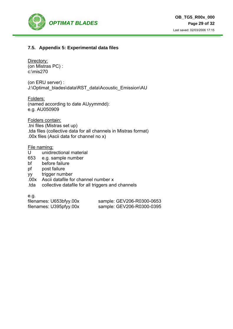
7.5. Appendix 5: Experimental data files Directory: (on Mistras PC) : c:\mis270 (on ERU server) : J:\Optimat_blades\data\RST_data\Acoustic_Emission\AU Folders: (named according to date AUyymmdd): e.g. AU050909 Folders contain: .tni files (Mistras set up) .tda files (collective data for all channels in Mistras format) .00x files (Ascii data for channel no x) File naming: U unidirectional material 653 e.g. sample number bf before failure pf post failure yy trigger number .00x Ascii datafile for channel number x .tda collective datafile for all triggers and channels e.g. filenames: U653bfyy.00x sample: GEV206-R0300-0653 filenames: U395pfyy.00x sample: GEV206-R0300-0395


Last saved: 02/03/2006 17:15

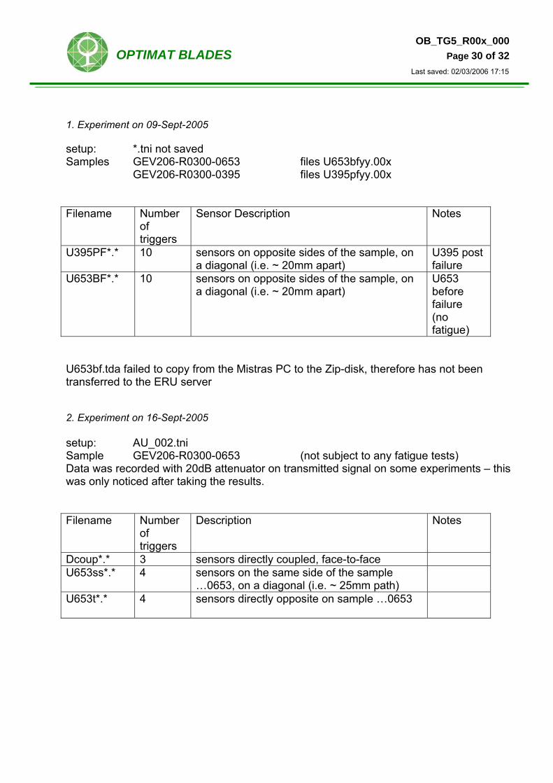
1. Experiment on 09-Sept-2005 setup: *.tni not saved Samples GEV206-R0300-0653 files U653bfyy.00x GEV206-R0300-0395 files U395pfyy.00x Filename Number

of triggers

Sensor Description Notes

U395PF*.* 10 sensors on opposite sides of the sample, on a diagonal (i.e. ~ 20mm apart)

U395 post failure

U653BF*.* 10 sensors on opposite sides of the sample, on a diagonal (i.e. ~ 20mm apart)

U653 before failure (no fatigue)

U653bf.tda failed to copy from the Mistras PC to the Zip-disk, therefore has not been transferred to the ERU server 2. Experiment on 16-Sept-2005 setup: AU_002.tni Sample GEV206-R0300-0653 (not subject to any fatigue tests) Data was recorded with 20dB attenuator on transmitted signal on some experiments – this was only noticed after taking the results. Filename Number

of triggers

Description Notes

Dcoup*.* 3 sensors directly coupled, face-to-face U653ss*.* 4 sensors on the same side of the sample

…0653, on a diagonal (i.e. ~ 25mm path)

U653t*.*

4 sensors directly opposite on sample …0653


Last saved: 02/03/2006 17:15

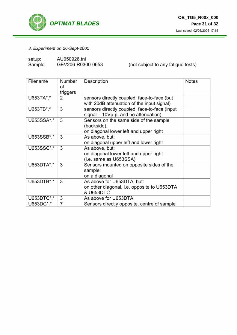
3. Experiment on 26-Sept-2005 setup: AU050926.tni Sample GEV206-R0300-0653 (not subject to any fatigue tests) Filename Number

of triggers

Description Notes

U653TA*.* 2 sensors directly coupled, face-to-face (but with 20dB attenuation of the input signal)

U653TB*.* 3 sensors directly coupled, face-to-face (input signal = 10Vp-p, and no attenuation)

U653SSA*.*

3 Sensors on the same side of the sample (backside), on diagonal lower left and upper right

U653SSB*.* 3 As above, but: on diagonal upper left and lower right

U653SSC*.* 3 As above, but: on diagonal lower left and upper right (i.e. same as U653SSA)

U653DTA*.* 3 Sensors mounted on opposite sides of the sample: on a diagonal

U653DTB*.* 3 As above for U653DTA, but: on other diagonal, i.e. opposite to U653DTA & U653DTC

U653DTC*.* 3 As above for U653DTA U653DC*.* 7 Sensors directly opposite, centre of sample


Last saved: 02/03/2006 17:15

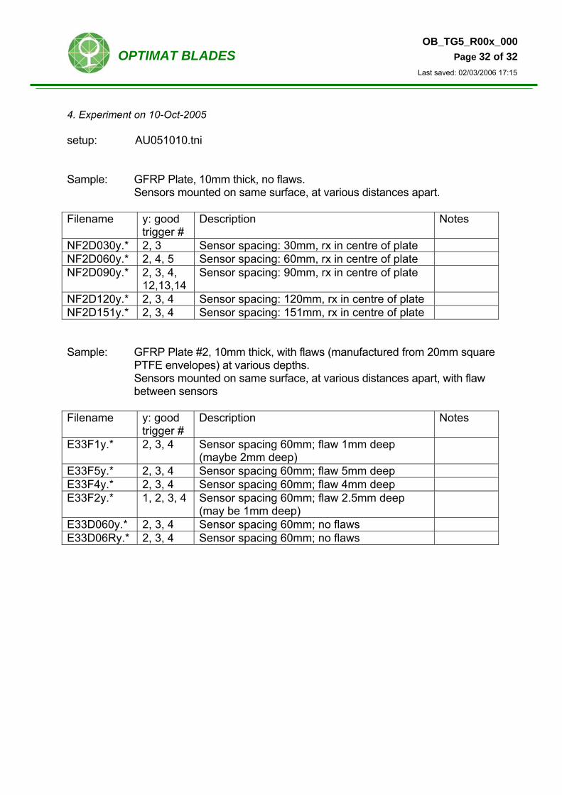
4. Experiment on 10-Oct-2005 setup: AU051010.tni Sample: GFRP Plate, 10mm thick, no flaws.

Sensors mounted on same surface, at various distances apart. Filename y: good

trigger # Description Notes

NF2D030y.* 2, 3 Sensor spacing: 30mm, rx in centre of plate NF2D060y.* 2, 4, 5 Sensor spacing: 60mm, rx in centre of plate NF2D090y.* 2, 3, 4,

12,13,14 Sensor spacing: 90mm, rx in centre of plate

NF2D120y.* 2, 3, 4 Sensor spacing: 120mm, rx in centre of plate NF2D151y.* 2, 3, 4 Sensor spacing: 151mm, rx in centre of plate Sample: GFRP Plate #2, 10mm thick, with flaws (manufactured from 20mm square

PTFE envelopes) at various depths. Sensors mounted on same surface, at various distances apart, with flaw between sensors

Filename y: good

trigger # Description Notes

E33F1y.* 2, 3, 4 Sensor spacing 60mm; flaw 1mm deep (maybe 2mm deep)

E33F5y.* 2, 3, 4 Sensor spacing 60mm; flaw 5mm deep E33F4y.* 2, 3, 4 Sensor spacing 60mm; flaw 4mm deep E33F2y.* 1, 2, 3, 4 Sensor spacing 60mm; flaw 2.5mm deep

(may be 1mm deep)

E33D060y.* 2, 3, 4 Sensor spacing 60mm; no flaws E33D06Ry.* 2, 3, 4 Sensor spacing 60mm; no flaws

Documents

The use of acousto-ultrasonic techniques to measure ... · PDF fileThe use of acousto-ultrasonic techniques to measure propagation time through glass-fibre reinforced coupons T TG