Embed Size (px)
Citation preview
University
International Studies Program
Growth and Equity Tradeoff in Decentralization Policy: China's Experience
B.Qiao, J. Martinez-Vazquez, and Y. Xu
Andrew YoungSchool of Policy Studies
Working Paper 02-16 July 2002
Georgia StateUniversity
International Studies Program Andrew Young School of Policy Studies Georgia State University Atlanta, Georgia 30303 United States of America Phone: (404) 651-1144 Fax: (404) 651-3996 Email: [email protected] Internet: http://isp-aysps.gsu.edu Copyright 2001, the Andrew Young School of Policy Studies, Georgia State University. No part of the material protected by this copyright notice may be reproduced or utilized in any form or by any means without prior written permission from the copyright owner.
Growth and Equity Tradeoffin Decentralization Policy: China's Experience
Working Paper 02-16
Baoyun Qiao, Jorge Martinez-Vazquez, and Yongsheng Xu July 2002

International Studies Program Andrew Young School of Policy Studies The Andrew Young School of Policy Studies was established at Georgia State University with the objective of promoting excellence in the design, implementation, and evaluation of public policy. In addition to two academic departments (economics and public administration), the Andrew Young School houses seven leading research centers and policy programs, including the International Studies Program. The mission of the International Studies Program is to provide academic and professional training, applied research, and technical assistance in support of sound public policy and sustainable economic growth in developing and transitional economies. The International Studies Program at the Andrew Young School of Policy Studies is recognized worldwide for its efforts in support of economic and public policy reforms through technical assistance and training around the world. This reputation has been built serving a diverse client base, including the World Bank, the U.S. Agency for International Development (USAID), the United Nations Development Programme (UNDP), finance ministries, government organizations, legislative bodies and private sector institutions. The success of the International Studies Program reflects the breadth and depth of the in-house technical expertise that the International Studies Program can draw upon. The Andrew Young School's faculty are leading experts in economics and public policy and have authored books, published in major academic and technical journals, and have extensive experience in designing and implementing technical assistance and training programs. Andrew Young School faculty have been active in policy reform in over 40countries around the world. Our technical assistance strategy is not to merely provide technical prescriptions for policy reform, but to engage in a collaborative effort with the host government and donor agency to identify and analyze the issues at hand, arrive at policy solutions and implement reforms. The International Studies Program specializes in four broad policy areas:
� Fiscal policy, including tax reforms, public expenditure reviews, tax administration reform
� Fiscal decentralization, including fiscal decentralization reforms, design of intergovernmental transfer systems, urban government finance
� Budgeting and fiscal management, including local government budgeting, performance-based budgeting, capital budgeting, multi-year budgeting
� Economic analysis and revenue forecasting, including micro-simulation, time series forecasting,
For more information about our technical assistance activities and training programs, please visit our website at http://isp-aysps.gsu.edu or contact us by email at [email protected].
Growth And Equity Tradeoff in Decentralization Policy:
China's Experience*
Baoyun Qiao, Jorge Martinez-Vazquez, and Yongsheng Xu
Department of Economics
Andrew Young School of Policy Studies Georgia State University
Atlanta, GA 30303
July 2002
* We are grateful to Kelly Edmiston, Felix Rioja, Neven Valev and Zhihua Zhang for useful comments on an earlier version of the paper.
1
Growth And Equity Tradeoff in Decentralization Policy:
China's Experience
Abstract
The paper uses China’s recent experience to investigate the potential tradeoff between economic growth and regional equity in the design of fiscal decentralization policy. Although present in other countries, this policy tradeoff has been particularly relevant to China over the last two decades. We build a theoretical model of fiscal decentralization, where overall national economic growth and equity in the regional distribution of fiscal resources are the two objectives pursued by a benevolent policy maker. Solutions that emphasize regional equity tend to have larger central government expenditures and higher contribution to the central budget by the richer jurisdictions. The reverse is true for solutions emphasizing growth. The model is tested using panel data for 1985-98. We find that fiscal decentralization in China led to economic growth, but this relationship was non-linear. Decentralization also led to significant increases in regional inequality. Overall, the historical record shows that pushing for a more equitable distribution of fiscal resources across provinces in China is likely to lead to lower national economic growth. The tradeoff between economic growth and regional equity is the most important and difficult decision in intergovernmental fiscal reform currently facing the Chinese authorities.
Keywords: China, Fiscal Decentralization, Economic Growth, Regional Equity. JEL Classifications: H73, P21, P51, R11.
2
I. Introduction The fundamental objective behind China's economic reform starting in the early
1980s was to develop the country’s economy in view of the failure of the socialist
planning model. A basic premise of this strategy was to decentralize decision making
because local governments could allocate some of the available resources more
efficiently than the central government had done until then. Close to twenty years of
decentralization reforms have followed during which the share of central government
expenditure in the general public sector budget decreased from about half in the
beginning of the 1980's to a little over one-fourth in 1998. China's economic strategy
explicitly accepted that economic growth would not benefit all regions the same, but
would let at least some of them have more opportunity to catch up with the global
economy. As former leader Deng Xiaoping had put it: “Let part of us be richer first.”
The relationship between growth and equity in the distribution of income1 has
been widely discussed in the economics literature.2 There has been much less research
on the relationship between growth and inequality in the geographic distribution of
resources or fiscal disparities, though there has been a recent debate in the
decentralization literature as to whether fiscal decentralization accelerates or retards
economic growth.3 On the other hand, there seems to be a general agreement in the
decentralization literature that, all else being equal, unfettered fiscal decentralization can
lead to a concentration of resources in a few geographic locations. 4 Nevertheless, to our
1 Distribution of income is defined across the population as opposed to across regions. 2 The growing consensus is that there is a negative relationship between inequality and growth (Barro and Sala-I-Martin (1995)) and that initial inequality is detrimental to long-run growth (Benabou (1996)). 3 See for example Devarajan et al. (1996) and Qian and Weingast (1997). 4 See for example Prud'homme (1995) and Murphy, Libonatti, and Salinardi (1995).
3
knowledge no empirical analysis of the impact of decentralization on the geographical
distribution of resources has been done.
The purpose of this paper is two-fold. We first develop a theoretical model of
fiscal decentralization, where overall national economic growth and equity in the
distribution of fiscal resources among subnational governments are the two objectives
pursued by the policy maker, to examine the tradeoff between growth and equity in the
context of China's fiscal decentralization policy. The theoretical model allows us to
investigate the conditions under which a policy trade-off between these two objectives
arises. Second, we test the model predictions with data covering the 1985 to 1998 period
of fiscal decentralization in China.
The rest of the paper is organized as follows. Section 2 briefly reviews China's
decentralization policy over the last 20 years. Section 3 develops the theoretical model
and presents its implications. The empirical tests are conducted in Section 4. Section 5
concludes. Proofs of our formal results in Section 3 are organized in the Appendix.
II. Fiscal Decentralization in China
Fiscal decentralization has been one of the most important policy thrusts
undertaken by the Chinese government during the last two decades of economic reform
from planned socialism. Although far from being highly decentralized, at least by
conventional measures (Bahl (1999)), China has undergone considerable decentralization.
Decentralization has been shaped by the two major fiscal reform thrusts that took place
during this period. The first reform started in 1985, and became known as the "Fiscal
Responsibility System" (FRS), and the second reform started in 1994, and was termed as
the "Tax Sharing System" (TSS).
4
Historically, China had a centrally planned economy and unitary fiscal system in
its "Soviet Socialism" era. After several fiscal decentralization experiments in the 1978-
84 period, fiscal reforms started in earnest in 1985 with the FRS. The essence of the FRS
was a contracting system, whereby the central government allowed provincial
governments to retain part of the tax revenues remaining after the remittance of a fixed
sum to the central government for a certain period of time. A key aspect of the FRS was
that provincial governments could get more fiscal revenue by collecting more tax.5 On
the other hand, the FRS created several problems for the central government. For
example, to have a higher local economic growth, local governments could contribute
fewer fiscal resources to the central government.6 This could be the case if local
governments tried to slow the growth of budget revenues by giving local enterprises more
direct resources and incentives, such as tax exemptions frequently at the expense of
central government revenues. This weakness of the FRS eventually led to the decrease of
the central government share in total budgetary revenues and to a lower share of total
budgetary revenue in GDP. Extra-budgetary funds provided a way to shield tax
collections from the central government and also an alternative way to finance local
governments’ expenditure without the risk of an eventual claw-back by the central
government (Bahl (1999) and Wong (2000)). Extra-budgetary funds actually were used to
finance all types of local government expenditure needs.7
5 Jin, Qian and Weingast (1999) note the "market preserving" features of this reform. 6 Actually, the lack of strict tax laws and influence on the tax administration gave provincial governments power over their effective tax rates and actual tax bases, even if local governments did not have legal authority over either. 7 Wong (2000) argues that the piecemeal intergovernmental reform in China led to a mismatch between expenditure responsibilities and revenue sources at the local level. In this context extra-budgetary funds provided local governments with much needed protection based on "self-reliance". See also Hofman (1993).
5
Realizing these shortcomings of the FRS, the central government adopted the TSS
in 1994. Major goals of the TSS were to increase (i) the shares of government revenues in
GDP, and (ii) the share of central government revenue in the total budgetary revenue. The
key measures in the TSS included the introduction of a value added tax as the major
revenue source and the setting up of uniform tax-sharing rates for major taxes including
VAT, which replaced the previous fixed-amount remittance scheme in the FRS. An
important measure of the TSS was to split up the old tax service in two and set up a
national tax services (NTSs) in all provinces to collect central taxes and shared taxes, and
a separate local tax services (LTSs) for the collection of the taxes assigned to local
governments. The TSS thus provided better incentives for local governments through
separate tax administrations and through the removal of the ceiling imposed de facto by
the FRS on the increase of local revenues.
The two rounds of reforms significantly changed China's fiscal landscape
including the relationship between central and local governments and the relationship
between the public sector and non-public sector. The most salient features of this process
of change include the following:
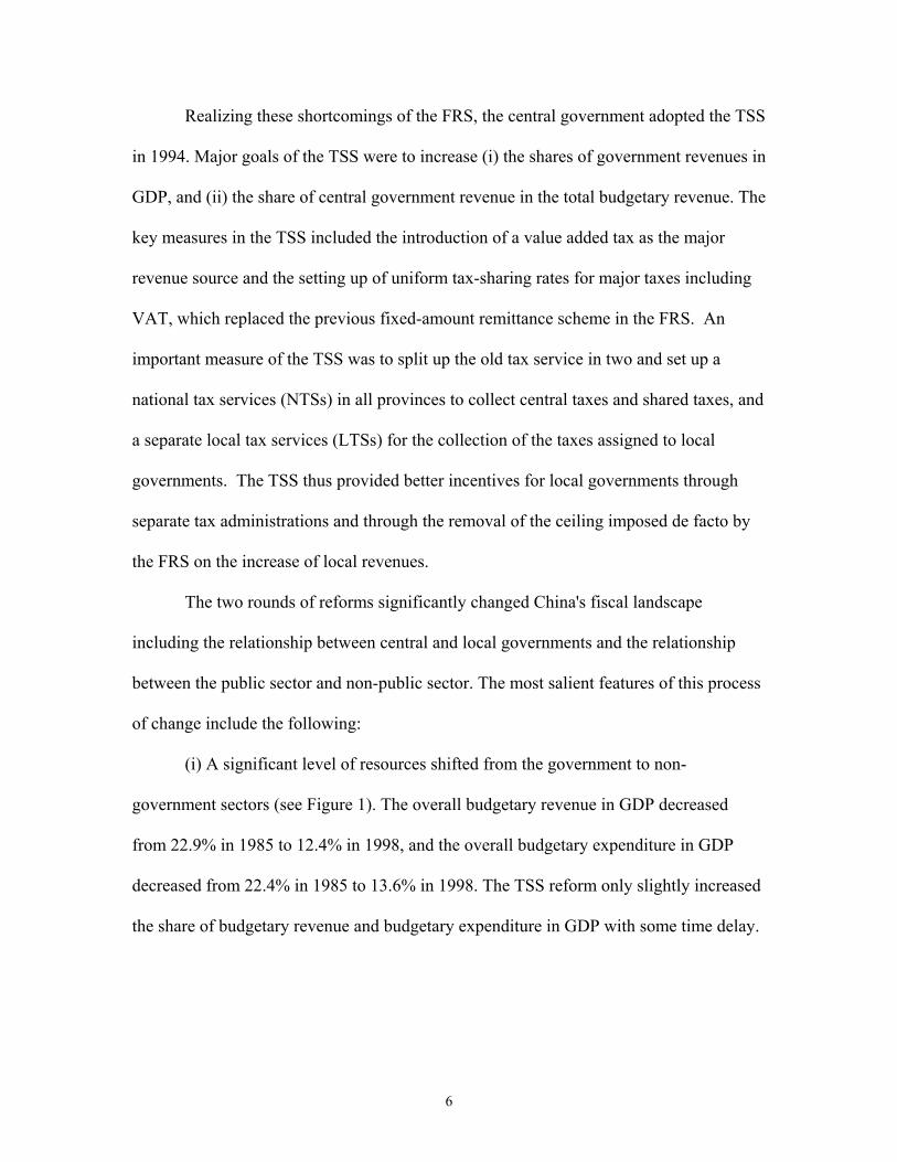
(i) A significant level of resources shifted from the government to non-
government sectors (see Figure 1). The overall budgetary revenue in GDP decreased
from 22.9% in 1985 to 12.4% in 1998, and the overall budgetary expenditure in GDP
decreased from 22.4% in 1985 to 13.6% in 1998. The TSS reform only slightly increased
the share of budgetary revenue and budgetary expenditure in GDP with some time delay.
6
(ii) More resources shifted from the central government to local governments (see
Figure 1). The share of local government budgetary expenditure in total government
budgetary expenditures increased from 60.3% in 1985 to 71.1% in 1998.
Note that after 1996, the share of local government expenditures decreased over
time but only slightly. 8
(iii) More resources at the subnational level shifted from the budget to extra-
budgetary funds (see Figure 1). The ratio of extra-budgetary expenditure to budgetary
expenditure of local governments kept increasing with only the exception of 19989.
Figure1: Share of Budgetary Expenditure Relative to GDP (SBER), Share of Local Budgetary Expenditure Relative to Total Budgetary Expenditure (SLBER), and Ratio of Extra-Budgetary Expenditure to Budgetary Expenditure (REBR), 1985-
1998
0.0
10.0
20.0
30.0
40.0
50.0
60.0
70.0
80.0
90.0
1985 1986 1987 1988 1989 1990 1991 1992 1993 1994 1995 1996 1997 1998
Year
%
SBER SLBER REBR
Because the main focus of this paper is on the potential tradeoff in fiscal
decentralization policy between the objectives of economic growth and equity in
8 The share of local government budgetary revenue in total government budgetary revenues shows a random trend because methods of calculating changed during the period. 9 The big downward jump in 1993 was not a real change but simply reflected a change in statistical methodology.
7
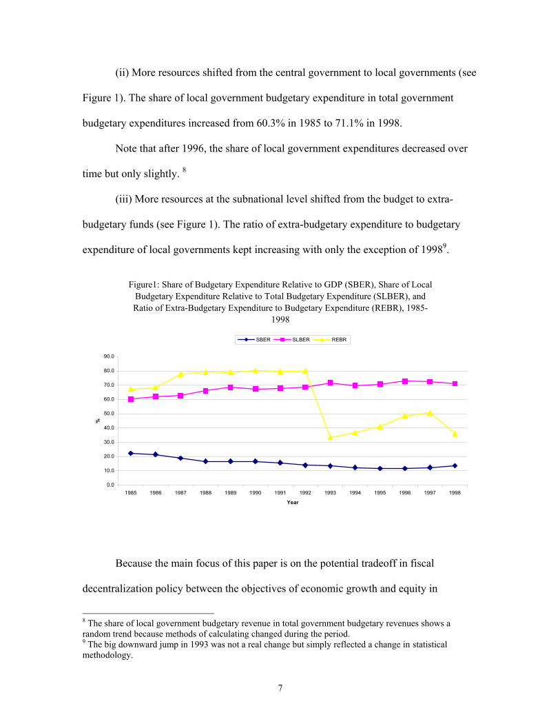
geographical distribution of fiscal resources, we also take a look at the performance of
China's system along those two dimensions. The rate of economic growth in China has
been quite high but changing during the sample period (see Figure 2).
Figure 2: Growth Rate of GDP from 1985 to 1998
0
2
4
6
8
10
12
14
16
1985 1986 1987 1988 1989 1990 1991 1992 1993 1994 1995 1996 1997 1998
Year
%
Inequality in the distribution of fiscal resources across provinces has tended to
increase over time as measured by the coefficient of variation (C.V.) of per capita
budgetary expenditure across provinces. Note that while the index decreased during the
FRS period, reaching the lowest value of 0.50 in 1992, it increased very quickly during
the TSS period and reached the highest value of 0.79 in 1997. In 1998 expenditure per
capita in Shanghai were over nine times larger than in Henan province.10
10 See Hofman and Yaset (1995) for a discussion of causes.
8
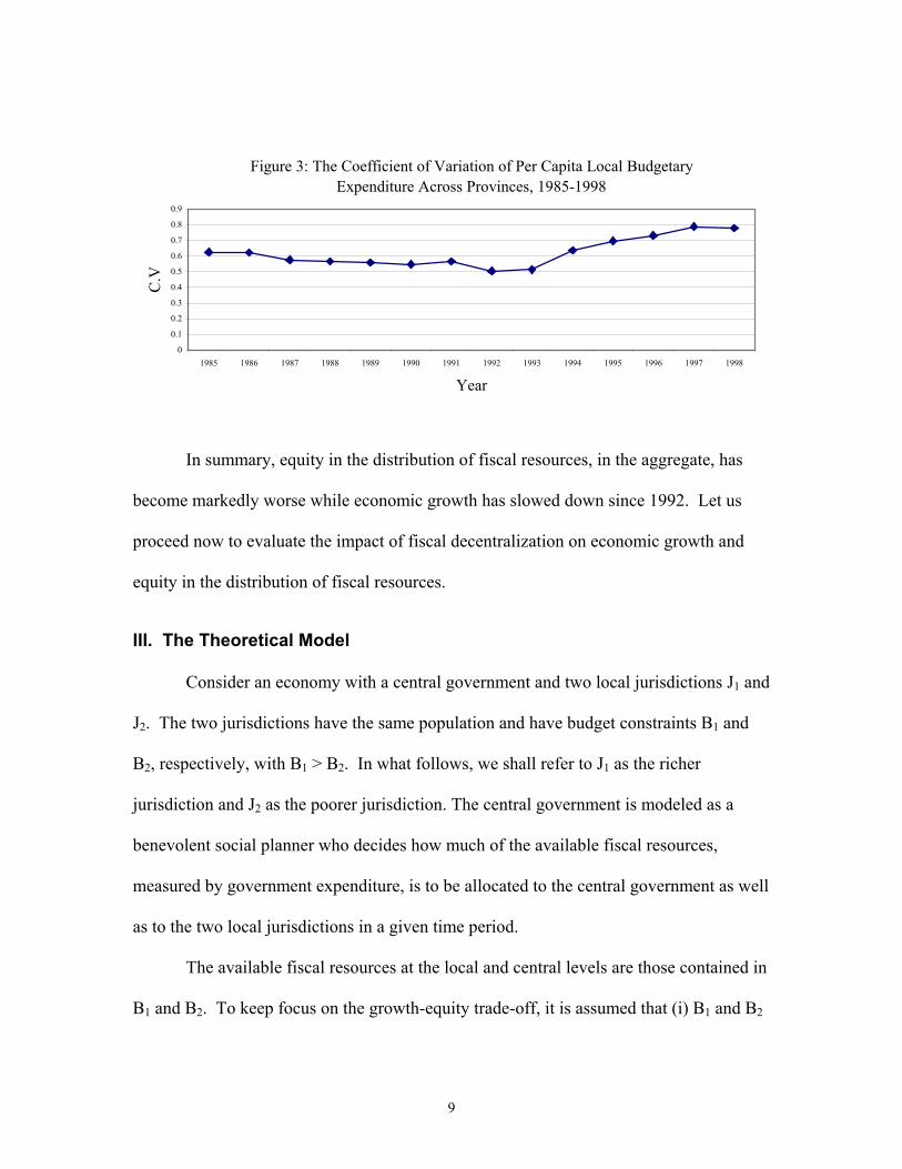
Figure 3: The Coefficient of Variation of Per Capita Local Budgetary Expenditure Across Provinces, 1985-1998
0
0.1
0.2
0.3
0.4
0.5
0.6
0.7
0.8
0.9
1985 1986 1987 1988 1989 1990 1991 1992 1993 1994 1995 1996 1997 1998
Year
C.V
In summary, equity in the distribution of fiscal resources, in the aggregate, has
become markedly worse while economic growth has slowed down since 1992. Let us
proceed now to evaluate the impact of fiscal decentralization on economic growth and
equity in the distribution of fiscal resources.
III. The Theoretical Model
Consider an economy with a central government and two local jurisdictions J1 and
J2. The two jurisdictions have the same population and have budget constraints B1 and
B2, respectively, with B1 > B2. In what follows, we shall refer to J1 as the richer
jurisdiction and J2 as the poorer jurisdiction. The central government is modeled as a
benevolent social planner who decides how much of the available fiscal resources,
measured by government expenditure, is to be allocated to the central government as well
as to the two local jurisdictions in a given time period.
The available fiscal resources at the local and central levels are those contained in
B1 and B2. To keep focus on the growth-equity trade-off, it is assumed that (i) B1 and B2
9
reflect the choices between public goods and private goods made by the social planner at
the central level, and (ii) B1 and B2 are fixed. 11
The available fiscal resources in B1 and B2 are allocated as follows: (i) a portion
goes to central government expenditure, denoted by C, (ii) the remainder goes to local
expenditures: L1 for jurisdiction J1 and L2 for jurisdiction J2. The central expenditure C is
assumed to be a pure public good, benefiting both local jurisdictions. Funding for central
expenditure comes from contributions by the two local jurisdictions with share α for J1
and, consequently, (1-α) for J2. Local fiscal expenditure Li is a local public good
generating benefits only for jurisdiction Ji, i∈1, 2, and equals the value of the budget
constraint of jurisdiction Bi net of its contribution to the central expenditure, or L1=B1-
αC, and L2=B2-(1-α)C. In our simplified context, fiscal decentralization is defined as a
decrease in the share of the central government expenditures in total government
expenditures, that is, a decrease in C.
We further assume that, due to the concern of fairness, the social planner restricts
the value of α to the following range: α≤(B1-B2+C)/2C and α≥B1/(B1+B2). The former
restriction tells us that at any central expenditure level, the richer jurisdiction always has
no less local fiscal resources than the poorer jurisdiction, while the latter says that the
richer jurisdiction’s contribution share of fiscal resources to the central governments is
not less than the share of its budgetary resources in total budgetary resources.
The social planner cares about two objectives: overall economic growth rate in the
country, and equity in the distribution of fiscal resources (public expenditures) between
11 Changing levels of taxes and government expenditures in the economy may be expected to affect economic growth. We abstract from those effects and concentrate instead on the effects of the decentralization of expenditure.
10
the two jurisdictions. More specifically, the social welfare function (of the social planner)
U is a function of g, the overall growth rate in the country as defined below, and E, the
normalized coefficient of equity in the distribution of fiscal expenditure which is also
defined below. For tractability, we will assume that U takes a linear form:
[ ] EwgU +=1
The coefficient, w, attached to the growth rate, g, in [1] reflects the benevolent
planner’s concern about growth vis-à-vis equity. In particular, we assume that w∈(0, ∞).
Thus, the higher the value of w, the more the central planner is concerned about growth
vis-à-vis equity. As w approaches infinity, the social planner cares only about growth.
The overall growth rate g in [1] is expressed by the equation g=p1g1+ p2g2, where
p1 and p2 are weights, with p1=G1/G and p2=G2/G, and where G represents total output in
the previous time period, and Gi represents output in each jurisdiction Ji, i∈1,2, also in the
previous time period. The growth function of local jurisdiction Ji, gi, i∈1, 2, is assumed to
be a function of central fiscal expenditures C, its local fiscal expenditure Li, its capital
growth rate ki, and its labor growth rate hi. Since L1 and L2 are functions of C and α, as
defined above, gi can be expressed in terms of C, α, ki, and hi. We assume that the capital
growth rate and the labor growth rate in both jurisdictions are exogenous and are not
affected by the fiscal policy change, i.e., central expenditure C and the respective
contribution shares to central expenditure, or ∂ki/∂C=0, ∂hi/∂C=0, ∂ki/∂α=0, ∂ hi/∂α=0,
i∈1, 2.12 Both g1 and g2 are strictly concave and have continuous second-order derivatives
with respect to C and α. In particular, we assume ∂2gi/∂C2<0, ∂2gi/∂α2<0, i∈1, 2. It
12 Again, this assumption is to allow us to focus alone on the role played by decentralization
11
follows that for the overall growth function g, we have ∂2g/∂C2<0, and ∂2g/∂α2<0. We
also assume ∂2g/(∂C∂α)≥0.
The equity term, E, in [1] is defined not in terms of outcomes, such as per capita
income or equal economic growth across different jurisdictions, but rather in terms of
opportunity. Equity in the geographical distribution of fiscal resources is formally
defined13 as E=-(L1-L2)/(L1+L2). When E=0, we have perfect equity in local
expenditures. Alternatively, E can be written as a function of C and α: E(C, α)=-[B1-B2-
(2α-1)C]/( B1+B2-C).
Note that, by definition, the equity function E is strictly increasing in each of α
and C. Given that α∈[(B1/(B1+B2), (B1-B2+C)/2C], it follows that E∈ [-(B1-B2)/(B1+B2)),
0].14 Clearly, for any C>0, when α=(B1-B2+C)/2C, E=0, and when α=(B1/(B1+B2), E=-
(B1/(B1+B2)). It can be shown that ∂E/∂C>015 for α∈[(B1/(B1+B2),(B1-B2+C)/2C) and
∂E/∂C=0 if α=(B1-B2+C)/2C.
III.1 The General Model
The social planner has perfect information about fiscal resources and growth functions
and solves the following maximization problem:
Problem [1]
13 This measure is derived from the sum of the negative value of the distance from the relative share of local fiscal resources in total local fiscal resources to the perfect equal share of local fiscal resource, or
( )[ ]{ } 2122
121∑
=
−+−=i
i LLLE . Since L1>L2, E can be written as=-(L1-L2)/(L1+L2).
14 From the definition of E, we know ∂E/∂α=2C/(L1+L2). For any C>0 and L1+L2>0, we have ∂E/∂α>0. If α=B1/(B1+B2), E=-(B1-B2)/(B1+B2). If α=(B1-B2+C)/2C>B1/(B1+B2) for C>0, E=0. 15 From the definition of E, we know ∂E/∂C=[2/(L1+L2)]/[α-L1/(L1+L2)]. For any L1+L2>0, and
B1/(B1+B2)<α<(B1-B2+C)/2C, we have ∂E/∂C>0. If α=(B1-B2+C)/2C, we have ∂E/∂C=0.
12
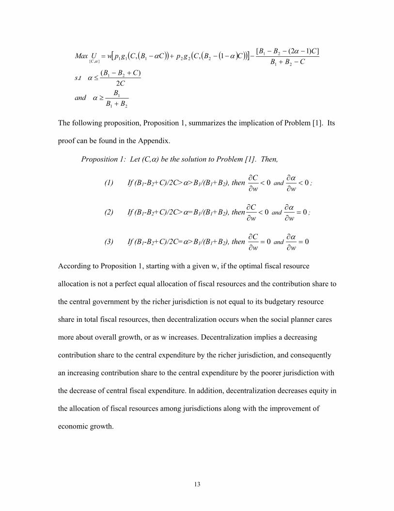
( )( ) ( )( )( )[ ]
21
1
21
21
21222111},{
2)(
.
])12([1,,
BBB
and
CCBB
ts
CBBCBB
CBCgpCBCgpwUMaxC
+≥
+−≤
−+−−−
−−−+−=
α
α
ααα
α
The following proposition, Proposition 1, summarizes the implication of Problem [1]. Its
proof can be found in the Appendix.
Proposition 1: Let (C,α) be the solution to Problem [1]. Then,
(1) If (B1-B2+C)/2C>α>B1/(B1+B2), then 0<∂∂
wC
and 0<∂∂
wα
;
(2) If (B1-B2+C)/2C>α=B1/(B1+B2), then 0<∂∂
wC
and 0=∂∂
wα
;
(3) If (B1-B2+C)/2C=α>B1/(B1+B2), then 0=∂∂
wC
and 0=∂∂
wα
According to Proposition 1, starting with a given w, if the optimal fiscal resource
allocation is not a perfect equal allocation of fiscal resources and the contribution share to
the central government by the richer jurisdiction is not equal to its budgetary resource
share in total fiscal resources, then decentralization occurs when the social planner cares
more about overall growth, or as w increases. Decentralization implies a decreasing
contribution share to the central expenditure by the richer jurisdiction, and consequently
an increasing contribution share to the central expenditure by the poorer jurisdiction with
the decrease of central fiscal expenditure. In addition, decentralization decreases equity in
the allocation of fiscal resources among jurisdictions along with the improvement of
economic growth.
13
On the other hand, starting with any given w, if the optimal resource allocation is
a perfect equal allocation of fiscal resources or if the contribution share to the central
government by the richer jurisdiction is equal to its budgetary resource share in total
fiscal resources, then the allocation of fiscal resources may not change when the social
planner cares more about the overall growth in the economy vis-à-vis equity in the
allocation of fiscal resources.
III.2. Special Cases We now discuss several special cases of our general model: (i) the best growth model in
which U = g; (ii) the given equity model in which E= Ē; (iii) the given growth rate model
in which g = ğ.
(i) The “best growth” model. The social planner in this case cares about the overall
growth rate only. This case is equivalent to the situation in which w becomes “very
large” in the general model. Viewed in this way, the optimal values of Cb and αb for the
best growth model can be obtained, respectively, from the optimal values of C and α of
the general model by allowing w approaches to ∞. From Proposition 1, Cg≥Cb and αg≥αb
hold. Further, the central government expenditure and the share of contribution to the
central expenditure by the richer jurisdiction reach their lowest values in the best growth
model.
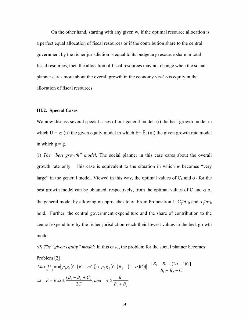
(ii) The "given equity” model: In this case, the problem for the social planner becomes:
Problem [2]
( )( ) ( )( )( )[ ]
21
121
21
21222111},{
,2
)(,.
])12([1,,
BBB
andC
CBBEEts
CBBCBB
CBCgpCBCgpwUMaxC
+≥
+−≤=
−+−−−
−−−+−=
−
αα
ααα
α
14
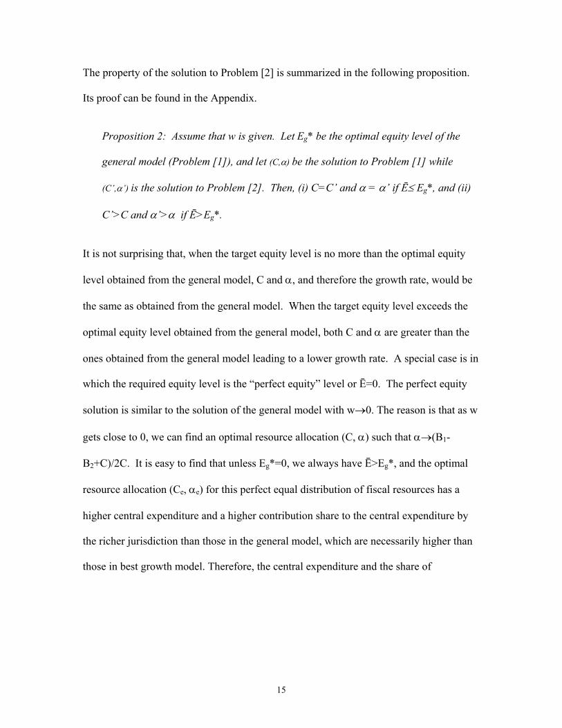
The property of the solution to Problem [2] is summarized in the following proposition.
Its proof can be found in the Appendix.
Proposition 2: Assume that w is given. Let Eg* be the optimal equity level of the
general model (Problem [1]), and let (C,α) be the solution to Problem [1] while
(C’,α’) is the solution to Problem [2]. Then, (i) C=C’ and α = α’ if Ē≤ Eg*, and (ii)
C’>C and α’>α if Ē>Eg*.
It is not surprising that, when the target equity level is no more than the optimal equity
level obtained from the general model, C and α, and therefore the growth rate, would be
the same as obtained from the general model. When the target equity level exceeds the
optimal equity level obtained from the general model, both C and α are greater than the
ones obtained from the general model leading to a lower growth rate. A special case is in
which the required equity level is the “perfect equity” level or Ē=0. The perfect equity
solution is similar to the solution of the general model with w→0. The reason is that as w
gets close to 0, we can find an optimal resource allocation (C, α) such that α→(B1-
B2+C)/2C. It is easy to find that unless Eg*=0, we always have Ē>Eg*, and the optimal
resource allocation (Ce, αe) for this perfect equal distribution of fiscal resources has a
higher central expenditure and a higher contribution share to the central expenditure by
the richer jurisdiction than those in the general model, which are necessarily higher than
those in best growth model. Therefore, the central expenditure and the share of
15
contribution to the central expenditure by the richer jurisdiction reach the highest level in
this perfect equity solution.16
(iii) The “given growth” model: In this case, the problem for the social planner becomes:
Problem [3]
( )( ) ( )( )( )[ ]
21
121
21
21222111},{
,2
)(,ð g .
])12([1,,
BBB
andC
CBBts
CBBCBB
CBCgpCBCgpwUMaxC
+≥
+−≤=
−+−−−
−−−+−=
αα
ααα
α
The property of the solution to Problem [3] is summarized in the following proposition.
Its proof can be found in the Appendix.
Proposition 3: Assume that w is given. Let gg
* be the optimal growth rate of the
general model (Problem [1]), and let (C,α) be the solution to Problem [1] while
(C’’,α’’) be the solution to Problem [3]. Then, (i) C=C’’ and α = α’’ if ğ ≤ gg*, and
(ii) C’’<C and α’’<α if ğ >gg*.
Therefore, to achieve a required growth level ğ, the optimal central government
expenditure C’’, the share of contribution to the central expenditure by the richer
jurisdiction α’’, and consequently, the overall growth rate and the equity level in the
given growth model are the same as those in the general model if ğ ≤ gg*. On the other
hand, any required growth rate ğ which is higher than the optimal growth rate in the
general model gg* will lead to less central expenditure C and smaller share of
16 It is worth stressing that Ē=0 in the given equity model differs from a model in which social planners pursue only perfect equity in the distribution of fiscal resource, or w=0. Assuming that the social planner wants to make a perfect equal distribution of fiscal resources between the two jurisdictions and does not care about the overall growth, given any central expenditure larger than zero, then it is easy to find that there exist multiple choices, or that the optimal condition is achieved for any central expenditure larger than zero by setting the value of α with α=(B1-B2+C)/2C. The social planner can pick any component in the set (C, α:"α"{α=(B1-B2+C)/2C, and C>0}) and achieve a perfect equity level in the distribution of fiscal resources.
16

contribution to the central government by the richer jurisdiction, α, and this policy results
in a lower level of equity in the distribution of fiscal resources to achieve the higher
growth rate ğ.
III. 3. A Summary
The results from the different models for C, α, the overall growth rate, and the
equity level are summarized in table 1
Table 1
Different Model Solutions
Model Name
Best growth
Given growth General model
Given equity
Perfect equity
Model g wğ+ E wg+E wg+Ē with Ē≠0 wg+Ē s.t Ē=0 Solution Cb, αb, gb, Eb Cğ , αğ, gğ, Eğ Cg,αg, gg, Eg CĒ , αĒ, gĒ, EĒ Ce, αe, ge, Ee
C Cb≤Cğ Cğ =Cg if ğ≤gg Cb<Cğ <Cg if gb>ğ >gg No solution if ğ>gb
Cğ≤Cg≤CĒ C=CĒ if Ē≤E C<CĒ if Ē>E
CĒ≤Ce
α αb ≤αğ αğ =αg if ğ≤gg αb<αğ <αg if gb>ğ >gg No solution if ğ>gb
αğ≤αg≤αĒ α=αĒ if Ē≤E α<αĒ if Ē>E
αĒ≤αe
Growth gb≥ gg gb>gğ >g if gb>ğ >gg
gğ =gg if ğ≤gg gğ =gb if ğ=gb No solution if ğ>gb
gğ ≥gg≥ gĒ g>gĒ if Ē>E g=gĒ if Ē≤E
gĒ≥ge
Equity Eb≤Eg Eg =Eg if ğ≤gg Eb<Eg<Eg if gb>ğ >gg No solution if ğ>gb
Eğ ≤Eg≤ EĒ E>EĒ if Ē>E E=EĒ if Ē≤E
EĒ≤Ee=0
The optimal resource allocation set, from the best growth solution, (Cb, αb), to the perfect
equity solution (Ce, αe), are presented graphically in Figure 4 below.
17
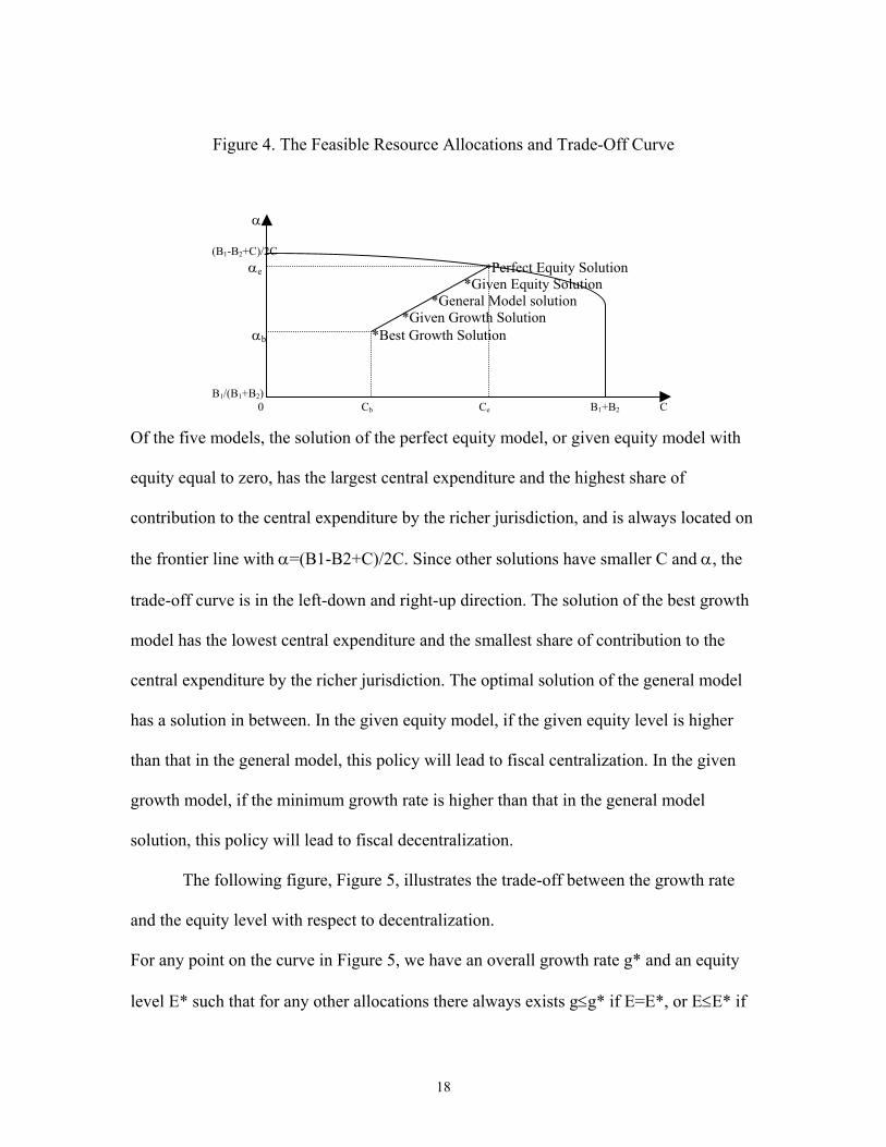
Figure 4. The Feasible Resource Allocations and Trade-Off Curve
Of the five models, the solution of the perfect equity model, or given equity model with
equity equal to zero, has the largest central expenditure and the highest share of
contribution to the central expenditure by the richer jurisdiction, and is always located on
the frontier line with α=(B1-B2+C)/2C. Since other solutions have smaller C and α, the
trade-off curve is in the left-down and right-up direction. The solution of the best growth
model has the lowest central expenditure and the smallest share of contribution to the
central expenditure by the richer jurisdiction. The optimal solution of the general model
has a solution in between. In the given equity model, if the given equity level is higher
than that in the general model, this policy will lead to fiscal centralization. In the given
growth model, if the minimum growth rate is higher than that in the general model
solution, this policy will lead to fiscal decentralization.
α (B1-B2+C)/2C αe *Perfect Equity Solution *Given Equity Solution *General Model solution *Given Growth Solution αb *Best Growth Solution B1/(B1+B2) 0 Cb Ce B1+B2 C
The following figure, Figure 5, illustrates the trade-off between the growth rate
and the equity level with respect to decentralization.
For any point on the curve in Figure 5, we have an overall growth rate g* and an equity
level E* such that for any other allocations there always exists g≤g* if E=E*, or E≤E* if
18
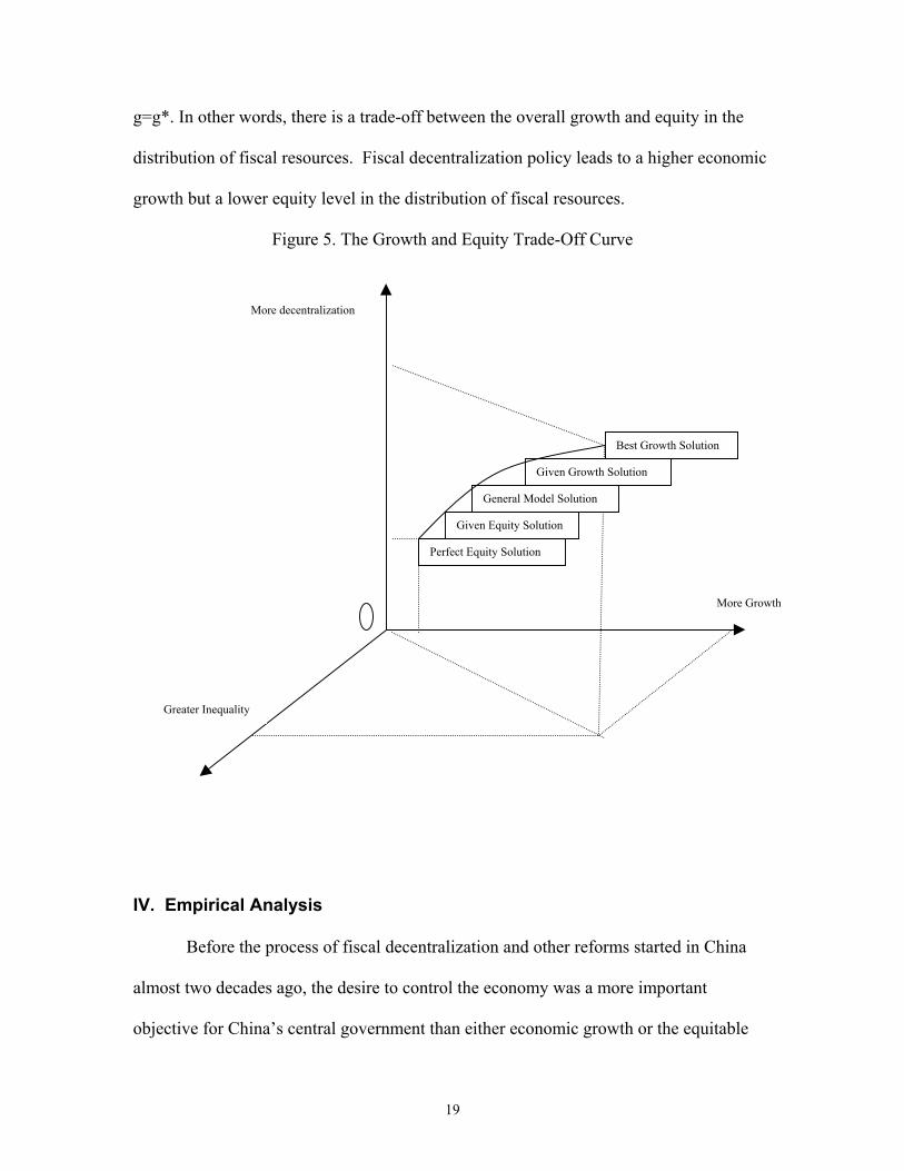
g=g*. In other words, there is a trade-off between the overall growth and equity in the
distribution of fiscal resources. Fiscal decentralization policy leads to a higher economic
growth but a lower equity level in the distribution of fiscal resources.
Figure 5. The Growth and Equity Trade-Off Curve
Greater Inequality
More Growth
Perfect Equity Solution
Given Equity Solution
General Model Solution
Given Growth Solution
Best Growth Solution
More decentralization
IV. Empirical Analysis
Before the process of fiscal decentralization and other reforms started in China
almost two decades ago, the desire to control the economy was a more important
objective for China’s central government than either economic growth or the equitable
19
distribution of fiscal resources. The political concern for social and economic control led
to an over-centralization of fiscal resources, and, to some extent as a side effect, to a
relatively equal distribution of fiscal resources. Decentralization was an obvious choice
of fiscal reform when economic growth became the most important goal for China’s
central government in the early 1980s.
Over the last two decades of fiscal reform, China’s economic growth arguably has
remained the most important goal for the central government. Economic growth provided
the moral justification for the continued decentralization policies that significantly
affected the allocation of fiscal resources in China. As we saw in section two, over the
last two decades China has experienced overall economic growth, but at the same time
the country has had to endure increasing fiscal disparities across local governments. Over
the past two decades, China’s decision makers appear to have been facing a fundamental
trade-off in decentralization policy between economic growth and equity in the
distribution of resources. Therefore, China's recent experience would seem to provide a
good case for testing the implications of our theoretical model.
Empirical Analysis
The empirical model: We use data for China from 1985 to 1998 to investigate the
impact of fiscal decentralization on growth and the geographical distribution of equity in
the allocation of fiscal resources, and whether there has been a trade-off between growth
and equity in China’s decentralization policy.
To allow for the potential simultaneous determination of economic growth and
the geographical distribution of fiscal resources, we use a simultaneous equation model
with economic growth and equity as dependent variables (see equations 4.3 and 4.4
20
below) and fiscal decentralization as the main explanatory variable of interest in both
equations. Based on our theoretical model, we expect decentralization to lead to
economic growth. However, all other things equal, more decentralization will not always
lead to a higher economic growth. To allow for a nonlinear relationship between fiscal
decentralization and growth, we introduce both fiscal decentralization and the square of
fiscal decentralization as explanatory variables in the growth equation of the model. As
the theoretical model predicts, a positive relationship between inequality in the
geographical distribution of fiscal resources and economic growth exists. This is based on
the premise, which seems to have been shared by Chinese decision makers, that some
provinces are better equipped and are likely to grow faster than others if economic
resources are left in those provinces.17
The measurements of fiscal decentralization and inequality in the geographical
distribution of fiscal resources require careful attention. Given the complexity of
decentralization in China, the issue of measuring the level of fiscal decentralization
presents something of a challenge. China’s decentralization has taken place on both the
revenue side and the expenditure side of the budget. Although far from perfect, we
choose the expenditure side as the basis for measuring decentralization. Fiscal revenues
in China are reallocated between central and local governments in a complex web of
flows (revenue sharing, rebates, many types of transfers, extra-budgetary funds and so
on), which tend to obscure the real fiscal resources available to the different government
17 This philosophy, again, was encapsulated in a famous phrase by Deng Xiaoping, the father of China's recent reforms: “Let part of us be richer first.”
21
levels. Fiscal decentralization is defined as the share of provincial fiscal expenditure18 in
total fiscal expenditure in per capita terms19, or:
(4.1)
t
t
it
it
it
it
it
POPCX
POPLX
POPLX
FD+
=
Where LXit stands for the provincial fiscal expenditure for province i in year t,
CXt stands for the central expenditure in year t, POPit stands for the population for
province i in year t, and POPt stands for the total population in year t. By this measure,
China experienced an increasing decentralization trend over time in the sample period. 20
We measure the inequality in the distribution of fiscal resources by:
1)2.4( −=t
itit PLX
PLXEQTY
where PLXit is the per capita fiscal expenditure in province i in year t, and PLXt is the
average per capita local fiscal expenditure across provinces for year t. This measure of
inequality is based on the concept of the relative share of fiscal resources. Let us, first,
define the ratio of the share of fiscal resources to the share of population of a region as
18 Provincial fiscal expenditure includes the consolidated expenditure of all sub-provincial governments (city, prefecture, county, and township governments). 19 The per capita measurement controls the impact of population on allocation of resources between the central and subnational governments. This measure is similar to the one used by Zhang and Zou (1998). 20 See, for example, Lin and Liu (2000). An alternative measure of decentralization is the marginal retention rate used by Jin, Qian and Weingast (1999). This latter measure focuses on the incentive response of local governments to decentralization. Our measure of decentralization better matches our research focus on the allocation of fiscal resources between the central and local governments. The issue with our measure is that there may be expenditures going through the provincial budgets, for which provincial governments do not have much discretion. In China, the central government uses guidelines and mandates for different types of local expenditures. Thus, the assumption of absolute authority by local governments over their expenditures does not hold entirely. However, we believe our proposed measure of fiscal decentralization is the best available for our purposes. At the very least, it captures changes in decentralization, with higher shares of provincial expenditure in total fiscal expenditure reflecting a move toward a more decentralized system.
22
the region’s relative share of fiscal resources. Then, the inequality measure in (4.2) is the
distance from the relative share to the perfect equal share. With perfect equality or an
ideal equity situation, the share of fiscal resources of a region is equal to the share of
population in the entire country or the relative share of fiscal resource equals one for all
regions in a given year. For provinces with an initial relative share of fiscal resources
higher than one, an increase in their share indicates that decentralization leads to a greater
inequality and a decrease in their share means a more equitable outcome. Similarly,
inequality increases if provinces with an initial relative share of less than 1 see their
shares decreased further, moving away from 1 due to decentralization. The larger the
distance in absolute terms, the higher the inequality in the inter-jurisdictional distribution
of fiscal resources.
We introduce several other explanatory variables in the growth equation, besides
the level of fiscal decentralization and the level of inter-jurisdictional inequality. The
first is a dummy variable for geographic location: access to sea-trade provides the east-
coast provinces of China with a higher development advantage over provinces in the
central and western areas of the country. Following the neoclassical tradition21, we
include the growth rates of capital (CPTL) and labor (LABR) as explanatory variables as
well. We include the effective tax rate at the provincial level (TAX) and its square
(TAX2) in the growth equation as proxies for the impact of the allocation of resources
between the public and private sectors on the growth rate. We also allow for the rate of
relative wealth on the growth equation, since the growth rate might be (inversely) related
21 See, for example, Barro (1990).
23
to the starting level of income22. For this purpose, we use the ratio of a province’s per
capita GDP to the average per capita GDP to measure the province's relative wealth.
Similarly, we use several other explanatory variables in the equity equation
besides the level of fiscal decentralization and the rate of economic growth. An
explanatory variable of particular interest is the subnational government's reliance on
extra-budgetary funds.23 Previous quantitative studies of decentralization in China either
treated extra-budgetary funds as exactly identical to ordinary budgetary expenditure (for
example, Zhang and Zou (1998)), or just ignored them (for example, Lin and Liu (1999)).
Since our research focuses on the distribution of all public resources, we use the ratio of
extra-budgetary expenditure to regular budgetary expenditure to control for how the
access or availability of this informal resource channel (extra-budgetary expenditure)
may affect equity in the distribution of budgetary resources. Provinces are not expected to
have equal access or potential use of extra-budgetary funds. Because extra-budgetary
funds are financed through a variety of fees (often illegal), we expect richer provinces to
be able to make wider use of this type of financing24.
Other explanatory variables introduced in the equity equation include: the growth
rate of the labor force to control for differences in labor resources, and the effective tax
rate to help capture any impact on equity from the tax side.
Finally, in both the growth equation and the equity equation, we introduce several
time period dummies. We use a year dummy for observations after 1994 in both
22 See, for example, Romer (1986). 23 Extra-budgetary accounts provide more flexibility and discretion in the use of the funds because their use usually lacks specificity and rarely contains detailed criteria (Wong 1998). Extra-budgetary accounts can also be used to shield tax collections from the revenue sharing agreements with the central government (Bahl 1999). 24 See Wong (1998).
24
equations to allow for the differential impact of the TSS reforms. In addition, we use
another year dummy to control for the change in the computation method for extra-
budgetary funds starting in 1993. This is necessary because the overall volume of extra-
budgetary funds decreased dramatically due to a new computational method introduced
that year.
Summarizing, our estimating simultaneous equation model can be expressed as:
,543210
876
52
432
210
)4.4(
)3.4(
ititititititit
itititit
itititititit
TAXLABRXBGTGRWFDEQTY
EQTYCPTLLABR
RWTAXTAXFDFDGRW
ναααααα
νβββ
ββββββ
++++++=
++++
+++++=
where i stands for region i, t stands for year t, and νij and ν1ij are the stochastic
disturbance terms. The variable definitions are summarized in table 2.
Table 2
Variables Definition Variable Definition GRW Percent growth rate of nominal per capita GDP FD Fiscal decentralization: Per capita provincial fiscal
expenditure as a percentage of total per capita fiscal expenditure,which is the sum of per capita central fiscal expenditure and per capita provincial expenditure.
EQTY Fiscal inequality: the absolute value of the difference betweenthe relative share of fiscal resource and 1. Relative share of fiscalresources is the ratio of the share of fiscal resource to the share of population.
TAX Tax rate: provincial total tax revenue as a percentage of totalprovincial GDP
RW Relative wealth: the ratio of per capita GDP over average percapita GDP
XBGT The ratio of extra-budgetary expenditure to budgetary expenditure
LABR Growth rate of labor
25
CPTL Growth rate of capital investment
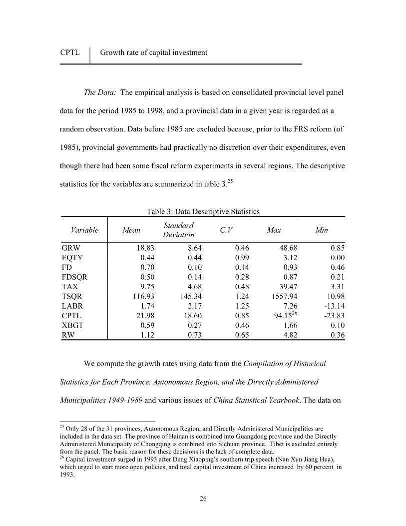
The Data: The empirical analysis is based on consolidated provincial level panel
data for the period 1985 to 1998, and a provincial data in a given year is regarded as a
random observation. Data before 1985 are excluded because, prior to the FRS reform (of
1985), provincial governments had practically no discretion over their expenditures, even
though there had been some fiscal reform experiments in several regions. The descriptive
statistics for the variables are summarized in table 3.25
Table 3: Data Descriptive Statistics
Variable Mean Standard Deviation C.V Max Min
GRW 18.83 8.64 0.46 48.68 0.85EQTY 0.44 0.44 0.99 3.12 0.00FD 0.70 0.10 0.14 0.93 0.46FDSQR 0.50 0.14 0.28 0.87 0.21TAX 9.75 4.68 0.48 39.47 3.31TSQR 116.93 145.34 1.24 1557.94 10.98LABR 1.74 2.17 1.25 7.26 -13.14CPTL 21.98 18.60 0.85 94.1526 -23.83XBGT 0.59 0.27 0.46 1.66 0.10RW 1.12 0.73 0.65 4.82 0.36
We compute the growth rates using data from the Compilation of Historical
Statistics for Each Province, Autonomous Region, and the Directly Administered
Municipalities 1949-1989 and various issues of China Statistical Yearbook. The data on
25 Only 28 of the 31 provinces, Autonomous Region, and Directly Administered Municipalities are included in the data set. The province of Hainan is combined into Guangdong province and the Directly Administered Municipality of Chongqing is combined into Sichuan province. Tibet is excluded entirely from the panel. The basic reason for these decisions is the lack of complete data. 26 Capital investment surged in 1993 after Deng Xiaoping’s southern trip speech (Nan Xun Jiang Hua), which urged to start more open policies, and total capital investment of China increased by 60 percent in 1993.
26
capital input and labor force growth are also taken from various issues of the China
Statistical Yearbook. Data on budgetary revenues and expenditures, and extra-budgetary
expenditure data are taken from Financial and Economic Statistical References, Fiscal
Statistics 1986-1991 and various issues of the China Statistical Yearbook. Data on
relative wealth are taken from the Compilation of Historical Statistics for Each Province,
Autonomous Region, and the Directly Administered Municipalities 1949-1989 and
various issues of China Statistical Yearbook.
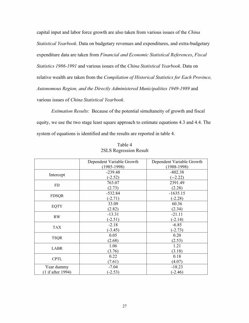
Estimation Results: Because of the potential simultaneity of growth and fiscal
equity, we use the two stage least square approach to estimate equations 4.3 and 4.4. The
system of equations is identified and the results are reported in table 4.
Table 4 2SLS Regression Result
Dependent Variable Growth (1985-1998)
Dependent Variable Growth (1988-1998)
Intercept -239.48 (-2.52)
-802.38 (--2.22)
FD 763.07 (2.73)
2391.49 (2.28)
FDSQR -532.84 (-2.71)
-1635.15 (-2.28)
EQTY 33.09 (2.82)
60.36 (2.34)
RW -13.31 (-2.51)
-21.11 (-2.14)
TAX -2.18 (-3.45)
-6.85 (-2.73)
TSQR 0.05 (2.68)
0.20 (2.53)
LABR 1.06 (3.76)
1.21 (3.18)
CPTL 0.22 (7.61)
0.18 (4.07)
Year dummy (1 if after 1994)
-7.04 (-2.53)
-18.23 (-2.46)
27
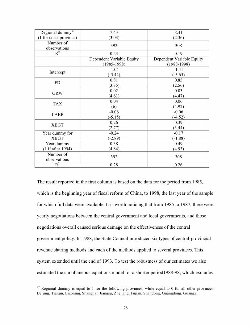
Regional dummy27 (1 for coast province)
7.43 (3.03)
8.41 (2.36)
Number of observations 392 308
R2 0.23 0.19
Dependent Variable Equity (1985-1998)
Dependent Variable Equity (1988-1998)
Intercept -1.04 (-5.42)
-1.41 (-5.65)
FD 0.81 (3.35)
0.85 (2.56)
GRW 0.02 (4.61)
0.03 (4.47)
TAX 0.04 (6)
0.06 (4.92)
LABR -0.06 (-5.15)
-0.06 (-4.52)
XBGT 0.26 (2.77)
0.39 (3.44)
Year dummy for XBGT
-0.24 (-2.89)
-0.17 (-1.88)
Year dummy (1 if after 1994)
0.38 (4.84)
0.49 (4.93)
Number of observations 392 308
R2 0.28 0.26
The result reported in the first column is based on the data for the period from 1985,
which is the beginning year of fiscal reform of China, to 1998, the last year of the sample
for which full data were available. It is worth noticing that from 1985 to 1987, there were
yearly negotiations between the central government and local governments, and those
negotiations overall caused serious damage on the effectiveness of the central
government policy. In 1988, the State Council introduced six types of central-provincial
revenue sharing methods and each of the methods applied to several provinces. This
system extended until the end of 1993. To test the robustness of our estimates we also
estimated the simultaneous equations model for a shorter period1988-98, which excludes
27 Regional dummy is equal to 1 for the following provinces, while equal to 0 for all other provinces: Beijing, Tianjin, Liaoning, Shanghai, Jiangsu, Zhejiang, Fujian, Shandong, Guangdong, Guangxi.
28
the years of strong local government bargaining. We find that the results for the period
1988-1998 are almost identical in sign with similar statistic significance. For both
estimations based on dataset 1985-1998 and 1988-1998, the Durbin-Watson tests show
no evidence that the true error disturbances are auto-correlated in our model. Meanwhile,
the Breusch-Pagan test rejects the null hypothesis of homoscedasticity; therefore, the t-
statistics in parentheses are based on heterokedasticity-consistent standard errors (White
1980). A description of the main results follows.
First, fiscal decentralization significantly affected economic growth. A higher
level of decentralization led to a higher rate of economic growth, but as expected, this
relationship was non-linear.28
Second, fiscal decentralization policies in China significantly increased
inequality in the distribution of fiscal resources. The coefficient of fiscal decentralization
in the equity equation is 0.81 and statistically significant. This provides statistical
support to the proposition of our theoretical model that a growth-oriented fiscal
decentralization policy leads to higher inequality in the distribution of fiscal resources.
Third, there was a positive relationship between inequality in the distribution of
fiscal resources and economic growth in both the growth and equity equations. From the
growth equation, the more unequal distribution of fiscal resources appeared to have
contributed positively to economic growth. In other words, an increase in equity in the
distribution of fiscal resources measured by a change of 0.01 in the equity coefficient
would have implied a sacrifice of 0.33 percent in economic growth at the margin. Based
28 The optimal level of fiscal decentralization for economic growth can be obtained by allowing for simultaneity and equating the first derivative to zero: for example for the 1985-1998 period, 763.07+33.09*0.81-2*532.84*FD = 0. The implied optimal level of fiscal decentralization for economic growth is 0.74 in the 1985-98 period and 0.75 in the 1988-98 period.
29

on the analysis of our theoretical model, this result suggests that local expenditures in
richer jurisdictions had over the sample period a higher marginal contribution to
economic growth than those of poorer jurisdictions. From the equity equation, we find
that the coefficient of economic growth is about 0.02 and highly significant. This means
that economic growth by itself contributed positively to the increase in fiscal inequality.
Approximately a 1 percent increase in economic growth implied a decrease of 0.02 in the
coefficient measuring equity in the distribution of fiscal resources.
As more fiscal resources shifted from poorer jurisdictions to richer jurisdictions,
overall economic growth improved, but at the same time the distribution of fiscal
resources became more unequal. Thus, the results confirm the proposition of our
theoretical model that the formulation of fiscal decentralization policy generally faces a
trade-off between economic growth and equity in the geographical distribution of fiscal
resources.
Fourth, the TSS reform of 1994 did not improve equity in the distribution of fiscal
resources, nor did it help with economic growth. The after-1994 year dummy is negative
and significant in the growth equation, and positive and significant in the equity equation.
The immediate government objectives of the 1994 fiscal reform were to improve “the
two ratios”: the ratio of fiscal revenue in GDP and the ratio of the central fiscal resources
in total fiscal resources. Therefore, this was fundamentally a re-centralization policy. But,
at least in our sample period through 1998, the ratio of the central fiscal resources in total
fiscal resources actually did not increase.
Fifth, the level of tax effort had a non-linear effect on economic growth. Too few
or too many resources shifted from the private sector to the public sector can be
30
detrimental to economic growth. This is shown by the negative and significant
coefficient for TAX and the positive and significant coefficient for TAX2 in the growth
equation.29
Sixth, a higher degree of reliance on extra-budgetary funds led to more
inequalities in the distribution of fiscal resources. This finding supports Wong’s (1998)
hypothesis that extra-budgetary funds are an important cause of fiscal inequality in
China.
Finally, the results for the economic growth equation in table 9 uphold the
neoclassical model of economic growth. As expected, the coefficients for capital and
labor growth are positive and statistically significant in the growth equation. The
negative relationship between growth and relative wealth also provides support for the
neoclassical proposition of income convergence.
V. Conclusion This paper investigates in the context of the Chinese economy the impact of fiscal
decentralization policy on economic growth and regional equity in the distribution of
fiscal resources, and the potential trade-offs between these two objectives. This policy
choice has been particularly relevant to China over the last two decades. While the rate of
economic growth in China has been quite high over approximately the last two decades,
inequality in the distribution of fiscal resources across local governments has increased
significantly. In recent years, it seems that the distribution of fiscal resources has become
markedly more unequal, while economic growth has slowed down.
29 By taking the first derivative with respect to TAX and equating it to zero:-2.18+33.09*0.04+0.05*2* TAX = 0, the optimal tax effort or effective tax rate implied by the data during the sample period is around9 percent. Recall that tax rate is defined as the provincial total tax revenue as a percentage of total provincial GDP.
31
The paper develops a theoretical model of fiscal decentralization, where overall
national economic growth and equity in the distribution of fiscal resources among
subnational governments are the two objectives pursued by the policy maker. The
theoretical model allows us to investigate under which conditions a policy trade-off
between the two objectives arises. Of the five models we investigate, the solution of the
best growth model has the lowest central expenditure and the smallest share of
contribution to the central expenditure by the richer jurisdiction. The solution of the
perfect equity model has the largest central expenditure and the highest share of
contribution to the central expenditure by the richer jurisdiction. The optimal solution of
the general model has a solution in between. In other words, we find a trade-off between
the overall economic growth and equity in the distribution of fiscal resources.
We test the model predictions with panel data covering the 1985 to 1998 period of
fiscal decentralization in China. Several findings are noteworthy.
First, fiscal decentralization significantly affected economic growth. A higher
level of decentralization led to higher growth, but as expected, this relationship was non-
linear. Second, decentralization policies in China led to significant increases in inequality
in the geographical distribution of fiscal resources. Third, from the estimated growth and
equity equations, inequality in the distribution of fiscal resources was positively related to
economic growth and higher economic growth led to more inequality. Fourth, during the
sample period that ends in 1998 the TSS reform did not improve equity in the
geographical distribution of fiscal resources, neither did it help much with economic
growth. Fifth, a higher degree of reliance on extra-budgetary funds led to more
inequalities in the distribution of fiscal resources.
32
It is hoped that the results in this paper can shed some light on the debate
regarding the impact of China’s decentralization policy on economic growth and the
distribution of fiscal resources across different regions. What to do about this trade-off
may represent the most important and difficult decision in intergovernmental fiscal
reform currently facing the Chinese authorities.
Even though the focus of this paper has been on China’s fiscal decentralization
experience, the impact of fiscal decentralization policy on economic growth and regional
equity and the trade-off between these two are important issues for many other countries
with active fiscal decentralization programs. Future research will reveal to what extent
our results for China are relevant to other countries with active decentralization policies.
33
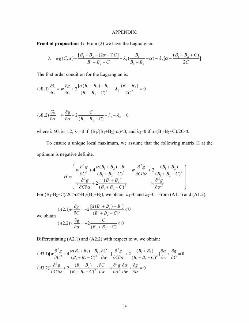
APPENDIX:
Proof of proposition 1: From (2) we have the Lagrangian:
]2
)([)(
])12([),( 21
221
11
21
21
CCBB
BBB
CBBCBB
Cwg+−
−−−+
−−+−−−
−= αλαλα
αλ
The first order condition for the Lagrangian is:
0)(
2)2.1(
02
)()(
])([2)1.1(
2121
221
2221
121
=−+−+
+∂∂
=∂∂
=−
−−+−+
+∂∂
=∂∂
λλαα
λα
CBBCgwA
CBB
CBBBBB
Cg
wC
A
λ
λ
where λi≥0, i∈1,2; λ1=0 if (B1/(B1+B2)-α)<0, and λ2=0 if α-(B1-B2+C)/2C<0.
To ensure a unique local maximum, we assume that the following matrix H at the
optimum is negative definite.
∂∂
−++
+∂∂
∂−+
++
∂∂∂
−+−+
+∂∂
=
2
2
221
212
221
212
321
1212
2
)()(2
)()(2
)()(4
αα
αα
gwCBB
BBC
gw
CBBBB
Cgw
CBBBBB
Cgw
H
For (B1-B2+C)/2C>α>B1/(B1+B2), we obtain λ1=0 and λ2=0. From (A1.1) and (A1.2),
we obtain 0
)(2)2.2(
0)(
])([2)1.2(
21
221
121
<−+
−=∂∂
<−+−+
−=∂∂
CBBCgwA
CBBBBB
CgwA
α
α
Differentiating (A2.1) and (A2.2) with respect to w, we obtain:
0])(
)(2)[2.3(
0])(
)(2[])(
)(4)[1.3(
2
2
221
212
221
212
321
1212
2
=∂∂
+∂∂
∂∂
+∂∂
−++
+∂∂
∂
=∂∂
+∂∂
−++
+∂∂
∂+
∂∂
−+−+
+∂∂
αα
αα
αα
α
gw
gwwC
CBBBB
CgA
Cg
wCBBBB
Cg
wC
CBBBBB
CgwA
34
Solving the simultaneous equations (A3.1) and (A3.2), we have:
||||)2.4(
||||)1.4(
2
1
HD
wA
HD
wCA
=∂∂
=∂∂
α
where
Cg
CBBBB
Cgwg
CBBBBB
CgwD
gCBB
BBC
gwCggwD
∂∂
−++
+∂∂
∂+
∂∂
−+−+
+∂∂
−=
∂∂
−++
+∂∂
∂+
∂∂
∂∂
−=
])(
)(2[]
)()(
4[||
])(
)(2[||
221
212
321
1212
2
2
221
212
2
2
1
ααα
ααα
Note that ∂g/∂C<0 and ∂g/∂α<0. Combining with our assumptions that H is negative
definite and that ∂2g/(∂C∂α)≥0, we obtain |D1|<0 and |D2|<0. Therefore, noting that |H|>0,
we obtain
0)2.5(
0)1.5(
<∂∂
<∂∂
wA
wCA
α
For α=B1/(B1+B2)<(B1-B2+C)/2C, λ2=0. From (A1.1), we obtain
0)(
])([2)1.6( 2
21
121 <−+−+
−=∂∂
CBBBBB
CgwA
α
Differentiating (A6.1) with respect to w, noting that α=B1/(B1+B2) (and hence 0=∂∂
wα
),
we obtain
0])(
)(4)[1.7( 3
21
1212
2
=∂∂
+∂∂
−+−+
+∂∂
Cg
wC
CBBBBB
CgwA
α
Given our assumption that H is negative definite, from (A6.1), clearly, 0<∂∂
wC
.
35

Finally, for α=(B1-B2+C)/2C> B1/(B1+B2), we obtain 2αC=B1-B2+C. Therefore, the
objective function in this case becomes )2
,( 21
CCBBCwg +− and the first order condition
becomes: 0]2
[ 221 =∂∂−
−∂∂
αg
CBB
Cgw . It is then clear that in this case, 0=
∂∂
wC and 0=
∂∂
wα
.
Proof of Proposition 2: The Lagrangian for the maximization problem given an equity
level can be written as:
Ε−+−
−−−+
−−+−−−
+−= λαλαλα
λα ]2
)([)(])12([)1(),( 212
21
11
21
21
CCBB
BBB
CBBCBBCwgλ
The first order condition is:
0)(
])12([)3.1(
0)(
)1(2)2.1(
02
)()(
])([)1(2)1.1(
21
21
2121
221
22
21
121
≤−+−−−
+Ε
=−+−+
++∂∂
=∂∂
=−
−−+−+
++∂∂
=∂∂
CBBCBB
B
CBBCgwB
CBB
CBBBBB
Cgw
CB
α
λλλαα
λα
λ
λ
λ
where λ≥0, λi≥0, i∈1,2; λ=0 if Ē+[B1-B2-(2α-1)C]/( B1+B2-C)<0, λ1=0 if [B1/(B1+B2)-
α]<0, and λ2=0 if α-(B1- B2+C)/2C<0.
(B1.1) and (B1.2) can be written as:
0)(
2')2.2(
02
)()(
])([2')1.2(
'2
'1
21
221'
2221
121
=−+−+
+∂∂
=−
−−+−+
+∂∂
λλα
λα
CBBCgwB
CBB
CBBBBB
CgwB
where λ+
=1
' ww , λ
λλ
+=
11'
1 , λ
λλ
+=
12'
2 .
If Ē+[B1-B2-(2α-1)C]/( B1+B2-C)=0, then λ≥0. It is clear that ww ≤' . From Proposition
1, by comparing (B2.1) and (B2.2) with (A1.1) and (A1.2), we obtain that the optimal
36

pair (C,α) for this case is no less than the optimal pair (C,α) for the general case. If
Ē+[B1-B2-(2α-1)C]/( B1+B2-C)<0, the first order condition becomes:
0)(
2)2.3(
02
)()(
])([2)1.3(
2121
221
2221
121
=−+−+
+∂∂
=∂∂
=−
−−−+−+
+∂∂
=∂∂
λλαα
λα
CBBCgwB
CBB
CBBBBB
Cgw
CB
λ
λ
which is exactly the same as the optimal condition in the general model.
Proof of Proposition 3: The first order condition for the maximization problem given a
growth rate can be expressed as follows:
0)3.1(
0)(
2)()2.1(
02
)()(
])([2)()1.1(
2121
221
2221
121
≤−
=−+−+
+∂∂
+=∂∂
=−
−−+−+
+∂∂
+=∂∂
ggC
CBBCgwC
CBB
CBBBBB
Cgw
CC
λλα
λα
λα
λ
λ
λ
where λ≥0, λi≥0, i∈1,2; λ=0 if g(g1,g2)-ğ >0; λ1=0 if (B1/(B1+B2)-α)<0; and λ2=0 if α-
(B1- B2+C)/2C<0.
Noting that ww ≥+ λ , by following similar arguments as in the proof of
Proposition 2, we obtain Proposition 3.
37
References Bahl, Roy W. 1999. Fiscal Policy in China: Taxation and Intergovernmental
Fiscal Relations. The 1990 Institute. Barro, Robert. 1990. Government Spending in A Simple Model of Endogenous
Growth. Journal of Political Economy 98: 103-25.
Barro, Robert., and Sala-I-Martin, X. 1995. Economic Growth. New York: McGraw-Hill.
Benabou, Roland. 1996. Inequality and Growth. In Ben S. Bernanke and Julio J. Rotemberg, eds. NBER Macroeconomics Annual 1996. Cambridge, MA: MIT Press. Devarajan, Shantayanan,Vinaya Swaroop and Heng-fu Zou. 1996. The
Composition of Public Expenditures and Economic Growth. Journal of Monetary Economics 37: 313-344.
Hofman, Bert. 1993. An Analysis of Chinese Fiscal Data over the Reform Period. China Economic Review 4(2): 213-30. Hofman, Bert and Shahid Yusef .1995. Budget Policy in China. In Reforming
China’s Public Finance, eds. Ehtisham Ahmad, Gao Qiang, and Vito Tanzi. Washington, D.C.:International Monetary Fund, pp. 35-48.
Jin, Hehui, Qian, Yingyi and Barry R. Weingast. 1999. Regional Decentralization
and Fiscal Incentives: Federalism, Chinese Style. Mimeo, presented at the Nobel Symposium on Transition, September.
Lin, Justin Yifu and Zhiqiang Liu. 2000. "Fiscal Decentralization and Economic
Growth in China. Economic Development and Cultural Change 49(1):1-22. Murphy, Richard Lopez, Oscar Libonatti, and Mario Salinardi. 1995. Overview
and Comparison of Fiscal Decentralization Experiences. In Richard Lopez Murphy (ed.), Fiscal Decentralization in Latin America. Washington, D.C.: Inter-American Development Bank: 1-57.
Prud'homme, Remy. 1995. On the Danger of Decentralization. World Bank Research Observer 10(2): 201-220. Qian, Yingyi and Barry R, Weingast. 1997. Federalism as A Commitment to
Preserving Market Incentives. The Journal of Economic Perspectives 11: 83-92. Romer, P. 1986. Increasing Returns and Long-run Growth. Journal of Political
Economy 94:1002-1037.
38
White, Herbert, "A Heteroskedasticity-Consistent Covariance Matrix Estimator and a Direct Test for Heteroskedasticity," Econometrica 48, May 1980, 817-38. Wong, Christine. 1998. Fiscal Dualism in China: Gradualist Reform and the Growth of Off-Budget Finance. In Donald Brean, Editor, Taxation in Modern China. New York: Routledge Press. Wong, Christine. 2000. Central-local Relations Revisited: the 1994 Tax-Sharing Reform and Public Expenditure Management in China. China Perspectives, Number 31, September – October. Zhang, Tao, and Heng-fu Zou. 1998. Fiscal Decentralization, Public Spending, and Economic Growth in China. Journal of Public Economics 67(2): 221-40.
39


![1809). (Lexington, KY) 1815-02-06 [p ]. - University …nyx.uky.edu/dips/xt744j09wf73/data/1236.pdfhouse, a handsome and general assortment of Merchandize, ("Purchased in Philadelphia](https://img.pdfslide.us/doc/110x75/5e93221c6099e27b7232f8e5/1809-lexington-ky-1815-02-06-p-university-nyxukyedudipsxt744j09wf73data1236pdf.jpg)