Embed Size (px)
Citation preview
In
International Center for Public Policy
Working Paper 14-19
January 2014
Estimating the Personal Income Distribution in
Spanish Municipalities
Using Tax Micro-Data
Miriam Hortas-Rico
Jorge Onrubia
Daniele Pacifico
INTERNATIONAL CENTER FOR
PUBLIC POLICY

International Center for Public Policy
Andrew Young School of Policy Studies
Georgia State University
Atlanta, Georgia 30303
United States of America
Phone: (404) 651-1144
Fax: (404) 651-4449
Email: [email protected]
Internet: http://aysps.gsu.edu/isp/index.html
Copyright 2006, the Andrew Young School of Policy Studies, Georgia State University. No part
of the material protected by this copyright notice may be reproduced or utilized in any form or by
any means without prior written permission from the copyright owner.
International Center for Public Policy Working Paper 14-19
Estimating the Personal Income Distribution in Spanish Municipalities Using Tax Micro-Data Miriam Hortas-Rico Jorge Onrubia Daniele Pacifico January 2014

International Center for Public Policy Andrew Young School of Policy Studies The Andrew Young School of Policy Studies was established at Georgia State University with the objective of promoting excellence in the design, implementation, and evaluation of public policy. In addition to two academic departments (economics and public administration), the Andrew Young School houses seven leading research centers and policy programs, including the International Center for Public Policy. The mission of the International Center for Public Policy is to provide academic and professional training, applied research, and technical assistance in support of sound public policy and sustainable economic growth in developing and transitional economies. The International Center for Public Policy at the Andrew Young School of Policy Studies is recognized worldwide for its efforts in support of economic and public policy reforms through technical assistance and training around the world. This reputation has been built serving a diverse client base, including the World Bank, the U.S. Agency for International Development (USAID), the United Nations Development Programme (UNDP), finance ministries, government organizations, legislative bodies and private sector institutions. The success of the International Center for Public Policy reflects the breadth and depth of the in-house technical expertise that the International Center for Public Policy can draw upon. The Andrew Young School's faculty are leading experts in economics and public policy and have authored books, published in major academic and technical journals, and have extensive experience in designing and implementing technical assistance and training programs. Andrew Young School faculty have been active in policy reform in over 40 countries around the world. Our technical assistance strategy is not to merely provide technical prescriptions for policy reform, but to engage in a collaborative effort with the host government and donor agency to identify and analyze the issues at hand, arrive at policy solutions and implement reforms. The International Center for Public Policy specializes in four broad policy areas: Fiscal policy, including tax reforms, public expenditure reviews, tax administration reform Fiscal decentralization, including fiscal decentralization reforms, design of intergovernmental
transfer systems, urban government finance Budgeting and fiscal management, including local government budgeting, performance-
based budgeting, capital budgeting, multi-year budgeting Economic analysis and revenue forecasting, including micro-simulation, time series
forecasting, For more information about our technical assistance activities and training programs, please visit our website at http://aysps.gsu.edu/isp/index.html or contact us by email at [email protected].
Estimating the Personal Income
Distribution in Spanish
Municipalities
Using Tax Micro-Data
Miriam Hortas-Rico
Jorge Onrubia
Complutense University of Madrid (Spain) & GEN (Governance and Economic Research Network).
Jorge Onrubia
Complutense University of Madrid (Spain) & GEN (Governance and Economic Research Network).
Daniele Pacifico
Department of the Treasury – Italian Ministry of Economy and Finance; Centre for North-South
Economic Research, University of Cagliari, Italy
Abstract
Local income data are an important economic indicator, widely used in a broad range of studies
related to regional convergence, urban economics, fiscal federalism, housing and spatial
analysis. Despite its importance, there is a lack of official data on local incomes and, most
importantly, on local income distributions. In this paper we use official data on personal income
tax returns and a reweighting procedure to derive a representative income sample at the local
level. Unlike previous attempts in the literature to acquire local income estimates, the results
obtained allow us to derive not only an average value for income but also its local distribution, a
valuable and informative tool for analysing distributional and income inequality. We apply this
methodology to Spanish Personal Income Tax micro-data and illustrate its potential use in
analysing income inequality by means of computed Gini, Atkinson indexes and top 0.01%,
0.5% and 0.01% income share measures for the most populated Spanish municipalities (those
with over 160,000 inhabitants).
Keywords: local income distribution, sample reweighting, income inequality, top incomes
JEL classification codes: C42, C61, D31, D63, O15
2 International Center for Public Policy Working Paper Series
1. Introduction
Which municipalities are richer than others? What are the causes of such differences? Is
there a pattern to the spatial distribution of local income? How do redistributive policies (such
as progressive taxation or transfer programmes) affect the income distribution across
municipalities? What is the impact of top income earners on economic growth and inequality?
Information on the local income distribution is essential in answering all these questions.
Local income data are therefore an important economic indicator, widely used in a
broad range of studies related to urban economics, fiscal federalism, housing and spatial
analysis, among others. In addition, aspects of income inequality and poverty at the local level
are receiving increasing attention from researchers in these areas. However, despite its
importance, local income data remain a key missing element within the official statistics of
many developed countries. The explanation lies, on the one hand, in the complexity of
designing surveys that are statistically reliable, and on the other hand, in the high cost of field
work, since it is necessary to carry out a large number of interviews in all the municipalities. As
a result, most of the household income and expenditure surveys have a limited territorial
representation, mainly at a regional or provincial level.
To redress this lack of information, a wide range of statistical techniques have been
developed over the last two decades aimed at providing reliable estimates of local income. The
majority often use micro-data information from surveys, combined with aggregate information
about relevant variables for the considered population subgroups. Haslett et al. (2010)
distinguish three main statistical methods with underlying similarities: small area estimation1,
imputation techniques2, and spatial micro-simulation modelling
3.
Household survey data have been used widely as the primary source for empirical
analysis on inequality, whereas little attention has been paid to income tax data. There is
however a growing body of empirical literature focusing on tax-based research (see for instance
Pikkety and Saez, 2003; Atkinson and Piketty, 2007; and Atkinson, Piketty and Saez, 2011).
The availability of personal income tax micro-data samples has also provided an attractive
method for modelling local income distributions. Although these samples have high population
1 Small area estimation refers to a set of techniques designed for improving sample survey estimates using
auxiliary information relating to analysed population subgroups. Some basic references on the
methodologies used for small area estimation are Rao (1999, 2003), and Elbers, Lanjouw and Leite
(2008). 2 Imputation techniques are used to incorporate observations and variables in the construction of
databases whose original information is either incomplete or has problems of sampling or no-response.
For further details on these techniques, see Kovar and Whitridge (1995). 3
Spatial micro-simulation modeling derives small area micro-data sets using reweighting techniques
usually based on optimisation procedures. For a further explanation on the extent and implementation of
these models, see for instance Rahman et al. (2010) and Tanton and Edwards (2013).
Estimating the Personal Income Distribution in Spanish Municipalities Using Tax Micro-Data 3
reliability, they are often statistically representative only at the regional level, as is the case in
Spain. In view of this limitation, it is necessary to develop a statistical treatment that allows us
to perform reliable income estimates for geographic areas below the regional level, i.e. the
municipalities. Hence in this paper we develop a model of sample reweighting designed to
overcome these problems, particularly in the context of distributional and income inequality
analysis4.
Thus the objectives of the paper are twofold. On the one hand, we seek to provide a
representative income sample at the local level based on official tax statistics. To that end, we
adapt a methodology for sample reweighting proposed in Deville and Särndal (1992), Creedy
(2003) and Creedy and Tuckwell (2004) to the case of Spanish micro-data of personal income
tax returns. In addition, we use this representative local income sample to derive local income
distributions. Unlike previous attempts to obtain local income estimates, in this paper we obtain
not only an average value of income for each Spanish municipality but also its local
distribution, allowing us to carry out income inequality analysis via certain inequality measures
such as Gini and Atkinson indexes. In addition, the data obtained allow us to study the top
incomes within each municipality, a topic of increasing interest within researchers using income
tax data at the country level (see for instance Atkinson, Piketty and Saez, 2011).
The article is organised as follows. In the next section we present the problem of
estimating personal income at the local level and we review the related literature and data
sources. The tax microdata-based model and the calibration approach implemented in the paper
to obtain the new sample weights used to derive local income distributions is presented in the
third section. The data used, the main findings and the validation of estimates are presented in
the fourth section. In the fifth section we report an illustration of income inequality analysis for
the case of Spain. Finally, in the last section, we conclude.
2. The problem of measuring local income: limitations and alternatives
2.1. State of the art
Most developed countries do not publish official statistics on personal or family income
at the local level nor the degree of inequality of their income distributions. This lack of
information represents an important limitation for economic analysis as these are variables
frequently used in applied economic research. There exists, however, a few exceptions in the
United States, United Kingdom or Australia.
4 Bramley and Smart (1996) conducted a pioneering study in this line, in which they obtained income
distributions for local districts of England using micro-data from the national Family Expenditure Survey.

4 International Center for Public Policy Working Paper Series
The U.S. case is probably the most remarkable one. The U.S. Bureau of Economic
Analysis provides data on personal income for the 366 metropolitan areas and their 3,113
counties, covering the period 1969-20115. Personal income is measured before the deduction of
personal income taxes and other personal taxes and is reported in current dollars, and it is
defined as the income received by all persons from all sources (the sum of net earnings by place
of residence, rental income, dividend and interest income, and current transfer receipts).
In the United Kingdom, estimations of the gross disposable household income
(henceforth GDHI) for the 139 local areas defined as NUTS3 (metropolitan and non-
metropolitan counties) are published by the Office for National Statistics (ONS) annually
(period 1997-2011). The most appropriate local indicators available are used and drawn from a
wide variety of survey and administrative sources. According to the National Accounts, GDHI
is defined as the amount of money that all of the individuals in the household sector have
available for spending or saving after current taxes on income and wealth, social contributions
paid and social benefits obtained.
In Australia, since 2005 the Bureau of Statistics has provided small area estimates of the
sources of personal income for each state and territory according to the various levels of the
Australian Standard Geographical Classification, including Local Government Areas. These
estimates, available for the years 1995-96 to 2010-11, are compiled using a combination of
individual income tax data from the Australian Taxation Office (wage and salary income, own
unincorporated business income, investment income, superannuation and annuity income and
other taxable income) and Government cash benefit income from the Commonwealth
Department of Family and Community Services.
Unlike the previous examples, in Spain, the National Statistical Office (henceforth INE)
does not provide data on family or personal income at the local level. Over the last decade,
several Regional Statistical Institutes (IDESCAT in Catalonia, EUSTAT in the Basque Country
or IAEST in Aragon, among others) have provided, though not always on a regular basis,
statistics including the per capita GDHI of those municipalities included in their jurisdictions. In
general, these are local estimates based on the Spanish Regional Accounts data provided by the
INE. The territorial imputation is carried out using indirect estimation methods. These methods
are based on econometric techniques that use the regional or provincial GDHI along with other
socioeconomic indicators available at the local level (i.e. total population, number of
unemployed residents, members of the population with a bachelor’s degree or higher, number of
vehicles registered, number of commercial and industrial establishments, average housing price,
5 For further details, visit http://www.bea.gov/regional/index.htm.
Estimating the Personal Income Distribution in Spanish Municipalities Using Tax Micro-Data 5
etc)6. Due to the lack of official statistics, the Lawrence R. Klein Research Institute
(Autonomous University of Madrid) has become the main source of local income data in Spain.
Certainly, there are many other estimates from the academic field that have also estimated the
municipal income, usually with a regional scope, using indirect methods to territorialise the
GDHI7.
The use of territorialised macroeconomic variables such as the gross value added
(henceforth GVA) or the GDHI to derive local income measures has two main limitations for
the analysis of personal income distributions. Firstly, these magnitudes do not adequately
represent the personal or household ability to pay taxes, nor the portion of income they can use
for consumption or savings, since they include capital income under the criteria of where
production activity is located instead of where their owners reside. For instance, we can think of
a residential municipality with a high standard of living where owners of businesses locate their
activities in other municipalities, even in other regions or countries. Of course, there will also be
municipalities whose residents do not have a high standard of living but where very profitable
companies are located, due to, for example, their lower wages. Another important limitation of
using macroeconomic aggregates to estimate local income is related to the impossibility of
obtaining distributions of income for municipalities, and consequently measures of inequality.
Whatever the statistical or econometric method used to estimate the per capita income of each
municipality, the result is a unique value, which makes it impossible to obtain information about
the dispersion of the magnitude.
The availability of micro data samples at the local level are essential in order to
compute inequality measures related to the personal income distribution of a municipality. As
far as we know, the U.S. Census Bureau is the only institution with experience in this regard. Its
American Community Survey (ACS) Public Use Microdata Sample (PUMS) provides annual
data on personal and family income8,9
.
6 Alternatively there are direct estimation methods based on the spatial localisation of the different
components of the gross disposable income from a production point of view. Their use is very rare given
the complexity of such imputation. 7
Among others, we can mention Arcarons et al. (1994) and Oliver et al. (1995) in Catalonia, Esteban and
Pedreño (1992) in Valencia Community, Fernández and Sierra (1992) in La Rioja, De las Heras (1992)
and De las Heras and Murillo (1998) in Cantabria, Herrero (1998) in Castile and Leon, Remírez-Prados
(1991) in Navarra, and Chasco y López (2004) in Murcia. Some of these introduce complex estimation
methods, such as multivariate factor and cluster analysis or econometric multiequational models.
Likewise, using spatial econometric techniques Alañón (2002) offers estimates of gross value added for
the Spanish municipalities, and Chasco (2003) and Buendía et al. (2012) obtain GDHI per capita
estimates for the Autonomy Community of Madrid and the Region of Murcia, respectively. 8 For this survey, total personal income is defined in terms of pre-tax income and includes the sum of the
amounts reported separately for wage or salary income, net self-employment income, interest, dividends,
net rental and royalty income, income from estates and trusts, social security or railway retirement
6 International Center for Public Policy Working Paper Series
Household surveys that include information on the income of their members are the
natural statistical source for providing micro-data on personal income. For the EU Member
States these surveys are The European Community Household Panel (ECHP), from 1994 to
2001 (eight waves), and The European Union Statistics on Income and Living Conditions (EU-
SILC) since 2003. Unlike their high quality level, guaranteed by the coordination and
supervision of Eurostat, their sampling design makes them invalid for estimates in smaller
territorial areas. A large number of survey interviews are required to meet an acceptable degree
of statistical representativeness at the municipal level. Thus the number of survey interviews
required would be greater than that needed at the regional or national level. This is why the lack
of available micro data for small areas is mainly a cost problem. In addition, misreporting and
income underreporting in expenditure and revenue surveys are substantive concerns that are
hard to mitigate10
. Moreover, as noted in Deaton (2003), personal income survey data show an
important underestimation when compared with equivalent magnitudes included in the National
Accounts, making them inappropriate for small area estimation11
.
2.2. Personal Income Tax returns as an alternative income data source
Tax returns on the Personal Income Tax (henceforth PIT) collected by national tax
administrations are an interesting alternative for overcoming the aforementioned territorial
representativeness limitations shown by household surveys for analysing personal income
distribution. As pointed out by Atkinson and Piketty (2007), the use of tax data for studying the
distribution of personal income goes far back in time12
. Nonetheless, in most OECD countries,
micro-level tax returns data sets are available only for the post-1970 or post-1980 period, except
for the United States, where the Internal Revenue Service (IRS) began releasing annual micro-
level data sets for income tax returns in 1960 (Atkinson and Piketty, 2007).
income, supplemental Security Income, public assistance or welfare payments, retirement, survivor, or
disability pensions, and all other income. 9 Currently, the ACS publishes single year data for all areas with populations of 65,000 or more. Among
the roughly 7,000 areas that meet this threshold are all states, all congressional districts, more than 700
counties, and more than 500 places. Areas with populations less than 65,000 will require the use of multi-
year estimates to reach an appropriate sample size for data publication. In 2008, the Census Bureau began
releasing 3-year estimates for areas with populations greater than 20,000. They also release the first 5-
year estimates for all census tracts and block groups from 2010. 10
Meyer and Sullivan (2011) evaluate the implications of these drawbacks for income inequality analysis.
Furthermore, Lohmann (2011) addresses the question of data collection in EU-SILC, finding a greater
reliability advantage in those countries that supplement the information from survey interviews using
administrative or register data for a wide range of variables, such as occurs in the Nordic countries. 11
Using a cross-country data set for developing and transitional economies, Ravallion (2003) analyses
how the national accounts deviates on average from mean household income or expenditure based on
national sample surveys. A detailed statistical study of these discrepancies is offered in Canberra Expert
Group’s Report (2001). 12
Early estimates date back to Bowley (1914) and Stamp (1916) for the United Kingdom, even though
the estimates made by Kuznets (1953, 1955) for United States can be considered as the pioneering income
distributions obtained using tax data.
Estimating the Personal Income Distribution in Spanish Municipalities Using Tax Micro-Data 7
The representativeness of these tax microdata is appropriate for small territorial
estimates, as in the case of municipalities. Generally, these annual PIT returns display
information about the different categories of taxable income: wage or salary income, retirement,
survivor, or disability pensions, some public assistance payments (including in some cases
unemployment benefits), net self-employment income and individual business income, interest,
dividends, royalty income, net rental, income from other estates and capital gains. In some
countries, imputed rent for homeowners and some exempt income are also included. The sum of
these variables can provide an adequate measurement of pre-tax income, in line with the one
presented in the ACS-PUMS (US Census Bureau).
Over the past decade, an increasing number of papers have focused their attention on
the concentration of income and wealth in top income earners (see Atkinson et al., 2011),
fostering the use of tax income data as a tool for personal income distribution analysis. In this
regard, it is important to notice that this tax definition of income is consistent with the notion of
ability to pay commonly used in microeconomic models (Piketty and Saez, 2003), besides
constituting a reasonable measurement of individual wellbeing (Leigh, 2007). In relation to the
reliability of tax data to measure personal income, as noted in Feldman and Slemrod (2007) and
Slemrod and Weber (2012), survey data are often not very credible due to the problem of
untruthful responses to delicate questions. Therefore income tax data are generally more
reliable, especially when personal income is measured from wages and salaries, pensions,
subsidies, interests and dividends, all of them withheld at the source of payment.
However, the estimation of personal income distributions using tax data also has some
conditioning factors. The unit of analysis is probably the most controversial issue (the
individual versus the family). However, as noted in Atkinson (2007), the individual approach is
useful when analysing personal income distributions and, as such, it has been commonly used in
the related literature on income inequality and redistribution. Of course, there are differences
when choosing the individual as the unit of analysis instead of the household, but these have to
be resolved by interpreting the results, without thereby having to give up the statistical
potentialities of the individual approach. Secondly, these data might be biased because of tax
evasion and avoidance. Nevertheless, Atkinson et al. (2011) point out that when tax data are
compared to other sources of information such as surveys, the influence of tax evasion and
avoidance on the distributive results is not large enough to mean that they should be rejected out
of hand. In this sense, Hurst et al. (2010) and Paulus (2013) also found a non-negligible income
underreporting by self-employed on income surveys compared to tax data.
8 International Center for Public Policy Working Paper Series
Thirdly, as noted above, the taxable income usually includes all incomes obtained by
residents in a territory regardless of its source. Ideally, one would like to measure the gross
income before any deductions or exemptions, even though this is not always possible. This is
due to the fact that available information comes from the tax forms according to the rules of
taxation. and as such, the income reported includes all essential components of personal income
in an economic sense, with the exception of certain exemptions of income that are not taxed.
Accordingly, the main limitation arises from the criteria for measuring certain kinds of incomes
taxed, as is the case of income from business activities (largely estimated by means of objective
methods), real estate imputed rents for homeowners, and capital gains. Despite this, when we
look at the measurement of aggregated household disposable income at the national level we
observe that it often offers lower income levels than the tax data13
. To sum up, we can say that
the aggregation of the different income components corresponds reasonably to gross income
before personal allowances and deductions are applied.
3. Tax microdata-based model
3.1. The model
Let ( ) be the personal income distribution (measured by the variable taxable income)
for a given year corresponding to the reference population . In turn, ( ) is the distribution
function of the same variable for the sample obtained from population administrative census of
tax returns.
For each of tax units, micro-data sample contains information on this income variable
and other variables of territorial identification, such as provincial or municipal codes. Insofar
the sample has been obtained using a particular sampling technique, a sample weight was
assigned to each observation extracted.
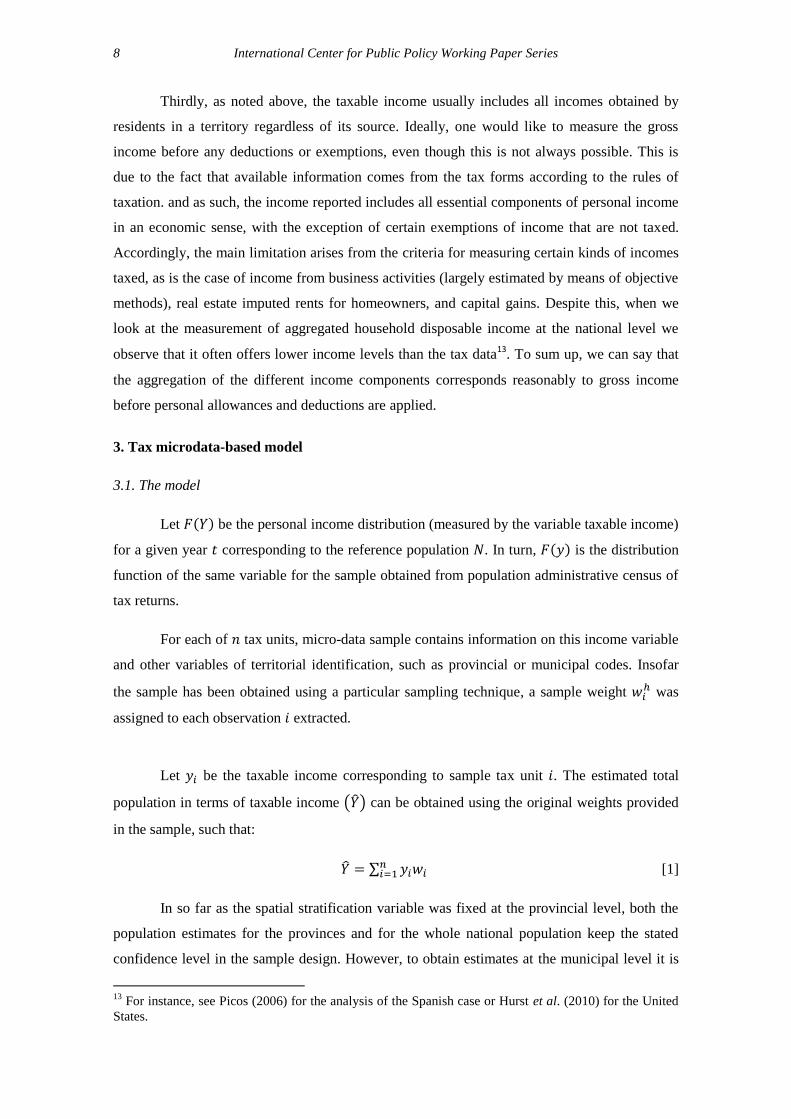
Let be the taxable income corresponding to sample tax unit . The estimated total
population in terms of taxable income ( ) can be obtained using the original weights provided
in the sample, such that:
∑ [1]
In so far as the spatial stratification variable was fixed at the provincial level, both the
population estimates for the provinces and for the whole national population keep the stated
confidence level in the sample design. However, to obtain estimates at the municipal level it is
13
For instance, see Picos (2006) for the analysis of the Spanish case or Hurst et al. (2010) for the United
States.
Estimating the Personal Income Distribution in Spanish Municipalities Using Tax Micro-Data 9
necessary to calculate new population weights, to the extent that our estimates would now face
smaller spatial areas used as a strata sample extraction.
We define this “new weight” as , such that the total population income estimated for
the municipality can be obtained as follows:
| ∑
[2]
Following Creedy and Tuckwell (2004), we use the distance criterion to assess the
closeness between and in each of spatial areas. In general terms, let denote this
distance through the function, ( ), what must verified in aggregate terms that:
( ) [3]
Therefore the method for obtaining the new weights that allow estimates of income at
the municipal level using a micro-data sample consists of solving the following optimisation
program: to minimise distance function [3] subject to municipality restriction [2]. To carry out
this reweighting we need information on true population totals for the taxable income variable
for each municipality, so that the estimated value | can be replaced in [2]. This information
is taken from the administrative census of personal income tax14
.
3.2. Computational settlement: the calibration approach
In this section we provide an overview of the method that we use to adjust the original
micro-data sample weights provided by the Spanish Tax Administration (henceforth AEAT) in
order to make them representative with respect to both the average income and the aggregate
number of taxpayers in each Spanish municipality. The methodology closely follows Creedy
(2003), Creedy and Tuckwell (2004) and Deville and Särndal (1992) and it was coded in Stata
12.
Following Creedy (2003), let us consider a sample of n taxpayers and K individual-level
variables, both monetary (as taxable income or tax liability) and non-monetary (as age, sex,
province and municipality of residence). We collect these variables for the generic taxpayer i in
the following vector: [ ] . If we define the original sample weight with the
vector [ ], the estimated population values of each K individual-level
variable is given by:
| ∑ [4]
14
These population data have been provided by Spanish Tax Administration Agency.
10 International Center for Public Policy Working Paper Series
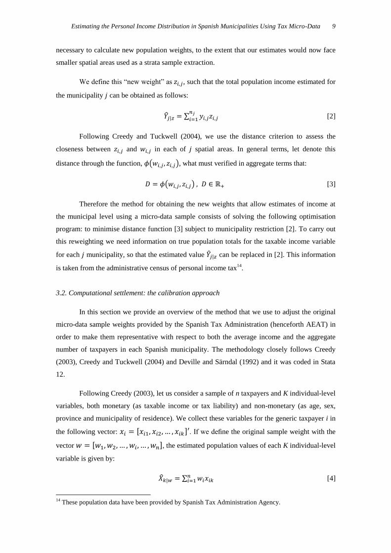
The AEAT provided us with the true population totals for some of these K
variables ( ). Specifically, we managed to obtain the aggregate income and the total number
of taxpayers in each j Spanish municipality from the AEAT. With this information in hand it is
possible to compute a new vector of sample weights for each municipality, [ ]
, where ∑ , that is as close as possible to the original sample weights, while
satisfying the set of K calibration equations:
∑
[5]
where is the true population value of each K individual-level variable in each j municipality.
Indeed, if we denote the distance between the original and the new sample weights with the
function ( ), the new sample weights can be obtained by minimising the following
Lagrangian function with respect to z:
∑ ( ) ∑ [ ∑
]
[6]
where are the Lagrange multipliers.
Clearly, the solution of the minimisation problem strongly depends on the property of
the distance function ( ), and in what follows we require the function ( ) to
respect two fundamental properties:
- The first derivative of ( ) with respect to must be expressed as a function of
the ratio between the new and the original weights:
( )
(
) [7]
- The inverse of the first derivative of ( ) must be explicitly invertible.
If these properties hold, then the n first order conditions for the problem in [6] are:
(
)
[8]
Then, we can obtain the new weights so that:
( ) [9]
and given a solution for the Lagrange multipliers, which can be obtained through an iterative
procedure (Newton’s method) after some algebraic manipulations of equations [9], [5]and [4].
1 2 Kλ = λ ,λ ,...,λ ´
Estimating the Personal Income Distribution in Spanish Municipalities Using Tax Micro-Data 11
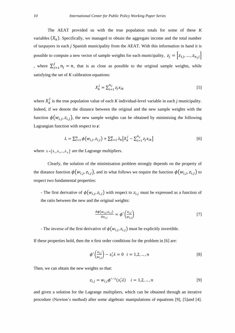
Specifically, if we substitute equation [9] into equation [5] and then subtract from both sides
equation [1], after certain rearrangements we obtain:
( | ) ∑ [ (
) ] [10]
The root of this function can be computed by means of the following iterative recursion:
( ) ( ) [ ( )
]
( ) [11]
where ( ) is given by the left hand side of equation [10] and, at each iteration I+1th, is
evaluated using the value of the Lagrange multipliers in the previous Ith iteration, λ[I]
. Hence,
given a set of initial values for λ, equation [11] can be repeatedly evaluated until convergence is
reached, where possible.
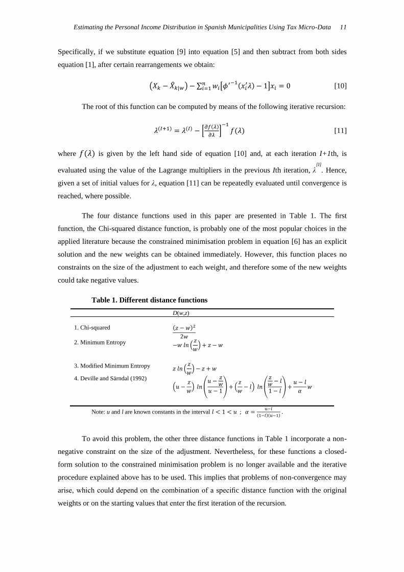
The four distance functions used in this paper are presented in Table 1. The first
function, the Chi-squared distance function, is probably one of the most popular choices in the
applied literature because the constrained minimisation problem in equation [6] has an explicit
solution and the new weights can be obtained immediately. However, this function places no
constraints on the size of the adjustment to each weight, and therefore some of the new weights
could take negative values.
Table 1. Different distance functions
D(w,z)
1. Chi-squared ( )
2. Minimum Entropy (
)
3. Modified Minimum Entropy (
)
4. Deville and Särndal (1992)
(
) (
) (
) (
)
Note: u and l are known constants in the interval
( )( )
To avoid this problem, the other three distance functions in Table 1 incorporate a non-
negative constraint on the size of the adjustment. Nevertheless, for these functions a closed-
form solution to the constrained minimisation problem is no longer available and the iterative
procedure explained above has to be used. This implies that problems of non-convergence may
arise, which could depend on the combination of a specific distance function with the original
weights or on the starting values that enter the first iteration of the recursion.
12 International Center for Public Policy Working Paper Series
Functions 2 and 3 force the new weight to be positive but they do not place an upper
bound to the adjustment. Hence implausible large weights with respect to the original ones
could result after the calibration process. This issue is considered by the fourth distance function
proposed by Deville and Särndal (1992), because it constrains the new weights within a user-
defined range. In particular, the ratio of the new to the original weight is bounded as follows:
[12]
where both l and u are known parameters that enter the distance function before the calibration
process15
.
4. Empirical results
4.1. Description of the Spanish municipal map
Spain is a decentralised country composed of three different levels of government: the
Central Government, 17 regional governments known as Autonomous Communities (created by
mandate of the Spanish Constitution in 1978) and some 8,110 Local Governments. As is shown
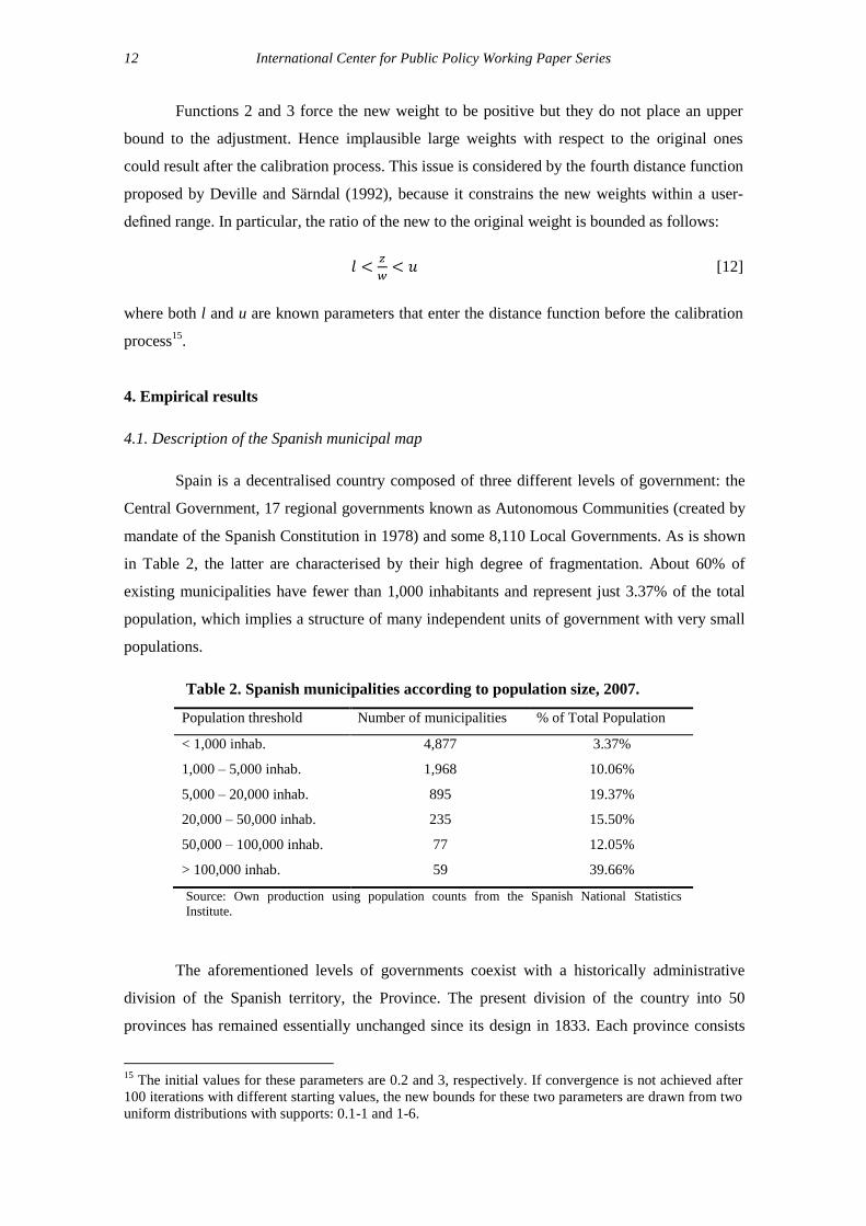
in Table 2, the latter are characterised by their high degree of fragmentation. About 60% of
existing municipalities have fewer than 1,000 inhabitants and represent just 3.37% of the total
population, which implies a structure of many independent units of government with very small
populations.
Table 2. Spanish municipalities according to population size, 2007.
Population threshold Number of municipalities % of Total Population
< 1,000 inhab. 4,877 3.37%
1,000 – 5,000 inhab. 1,968 10.06%
5,000 – 20,000 inhab. 895 19.37%
20,000 – 50,000 inhab. 235 15.50%
50,000 – 100,000 inhab. 77 12.05%
> 100,000 inhab. 59 39.66%
Source: Own production using population counts from the Spanish National Statistics
Institute.
The aforementioned levels of governments coexist with a historically administrative
division of the Spanish territory, the Province. The present division of the country into 50
provinces has remained essentially unchanged since its design in 1833. Each province consists
15
The initial values for these parameters are 0.2 and 3, respectively. If convergence is not achieved after
100 iterations with different starting values, the new bounds for these two parameters are drawn from two
uniform distributions with supports: 0.1-1 and 1-6.
Estimating the Personal Income Distribution in Spanish Municipalities Using Tax Micro-Data 13
of a group of municipalities, and one or more provinces yield to an Autonomous Community.
Central and Local Governments are formed according to direct election by universal suffrage
and subject to a proportional representation criterion, whereas governmental institutions at the
province level respond to the representation of political parties in each province’s
municipalities. That is to say, members of the Provincial Government are elected by the
municipal councillors among themselves.
4.2. The data
Micro-data (PIT, 2007). To carry out the estimate of local income distributions we use
micro-data contained in the annual Spanish PIT sample. In particular in this paper we use the
sample for the year 2007, which includes 1,351,802 records extracted from a population
providing 18,702,875 personal income tax returns (Picos et al., 2011). This database has been
developed by the Spanish Institute of Fiscal Studies (Instituto de Estudios Fiscales, IEF
henceforth), in collaboration with the Spanish National Tax Administration (Agencia Estatal de
Administración Tributaria - henceforth AEAT), the entity in charge of extracting annual
samples from its administrative registers of Spanish personal income tax16
.
For the construction of this annual sample the minimum variance stratification under
Neyman’s allocation method has been used. Thereby population income may be estimated in a
highly precise manner with a reasonable sample size. Three stratification variables have been
used in the sampling process: a) the province, as territorial stratum (48 provinces with common
fiscal regime, plus the Autonomous Cities of Ceuta and Melilla17
); b) the income level of the tax
filers (to that end, income sample places in 12 level)18
; c) the type of tax return (separate or joint
filing). Hence, the “original weight” is calculated for each observation as the ratio between the
size of the population of its belonging stratum and its corresponding sample size,
⁄ . To select the sample, the tax returns were classified in each one of the 1,152 strata
(48x12x2). Previously, the size of the total sample n was calculated for a specific relative
sampling error (e < 0.011) with a confidence level of 3 per 1,000. Next, the population for each
stratum (Nh) was determined using the population quasi-variance of the sample income for each
one of them (S2
h). Finally, using the values Nh and S2
h, the number of observations that had to be
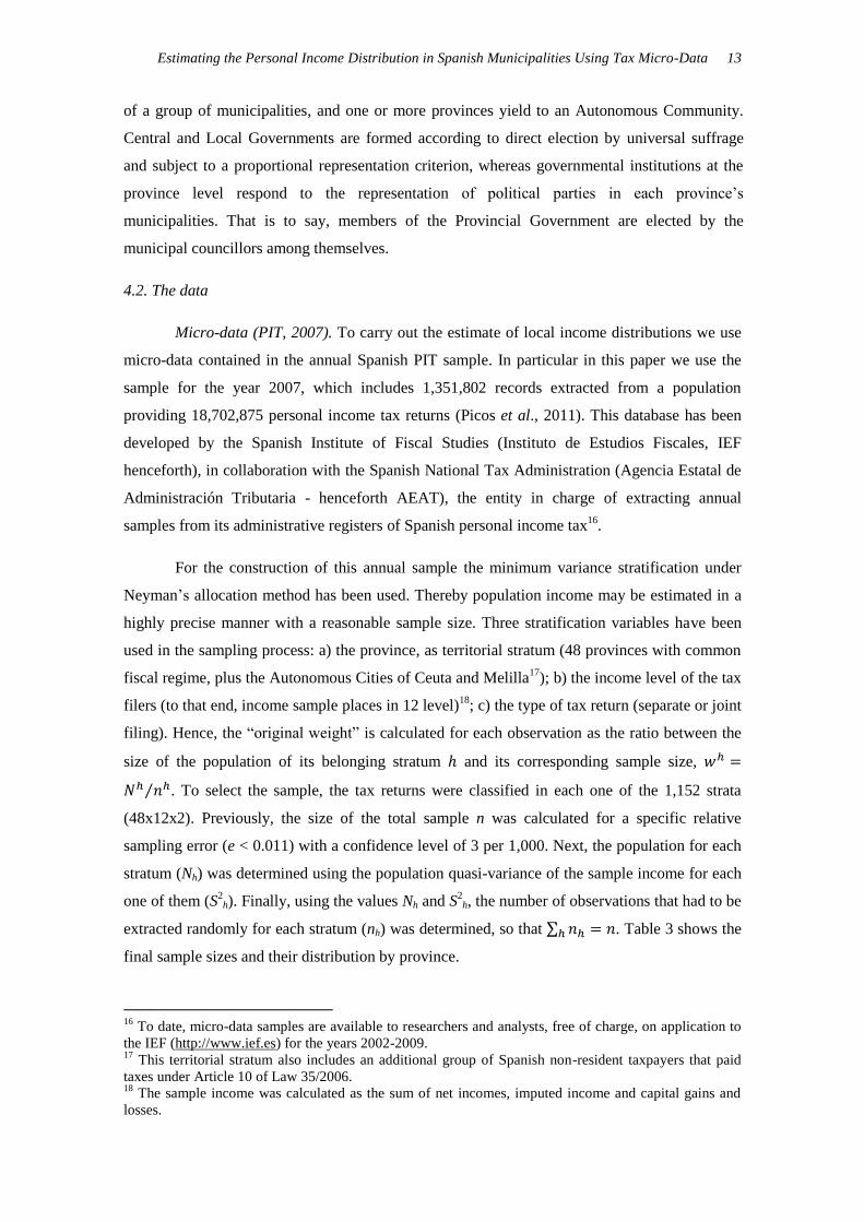
extracted randomly for each stratum (nh) was determined, so that ∑ . Table 3 shows the
final sample sizes and their distribution by province.
16
To date, micro-data samples are available to researchers and analysts, free of charge, on application to
the IEF (http://www.ief.es) for the years 2002-2009. 17
This territorial stratum also includes an additional group of Spanish non-resident taxpayers that paid
taxes under Article 10 of Law 35/2006. 18
The sample income was calculated as the sum of net incomes, imputed income and capital gains and
losses.
14 International Center for Public Policy Working Paper Series
Table 3. Final micro-data sample sizes and their distribution by province
Province Province Code Number of sample observations
(used in estimates)
Álava 1 -
Albacete 2 19,784
Alicante 3 44,072
Almería 4 24,353
Ávila 5 12,534
Badajoz 6 28,710
Balears (Illes) 7 32,885
Barcelona 8 86,880
Burgos 9 18,131
Cáceres 10 22,842
Cádiz 11 34,890
Castellón 12 25,682
Ciudad Real 13 21,542
Córdoba 14 33,076
Coruña (A) 15 37,749
Cuenca 16 14,172
Girona 17 24,974
Granada 18 33,254
Guadalajara 19 12,594
Guipúzcoa 20 -
Huelva 21 21,255
Huesca 22 14,167
Jaén 23 30,891
León 24 23,201
Lleida 25 20,342
Rioja (La) 26 16,820
Lugo 27 21,261
Madrid 28 110,208
Málaga 29 40,883
Murcia 30 38,140
Navarra 31 -
Ourense 32 19,439
Asturias 33 36,084
Palencia 34 12,065
Palmas (Las) 35 31,743
Pontevedra 36 33,238
Salamanca 37 18,651
Santa Cruz de Tenerife 38 30,891
Cantabria 39 23,579
Segovia 40 11,297
Sevilla 41 44,700
Soria 42 8,624
Tarragona 43 27,661
Teruel 44 11,822
Toledo 45 24,773
Valencia 46 53,361
Valladolid 47 22,904
Vizcaya 48 -
Zamora 49 14,452
Zaragoza 50 36,454
Ceuta 51 5,244
Melilla 52 5,068
Non residents 99 615
Total of observations 1,337,957
Source: own production using data drawn from the Spanish Personal Income Tax
2007 annual sample.
The original records provided by the AEAT are incorporated in a bi-dimensional file
that contains the PIT returns extracted using a sampling process (one per row). For each
Estimating the Personal Income Distribution in Spanish Municipalities Using Tax Micro-Data 15
observation the file offers a series of variables for which the source of information is, directly or
indirectly, the return form for the corresponding year19
.
Regarding territorial representation, the annual sample of micro-data includes tax
returns for 5,346 of the 7,024 Spanish municipalities, all of them belonging to the 15
Autonomous Communities with a common tax system (the database does not include
observations for the Basque Country and Navarra, which have their own tax systems (so-called
“foral tax systems”).
Using variables contained in the annual Spanish PIT sample for 2007, we establish the
definition of total personal income as the sum of the following items forming part of the gross
taxable income20
: salary and wage income, retirement pensions, general unemployment
subsidies, some non-exempt welfare payments and some disability pensions, net self-
employment income, interest, dividends, royalty income, survivor annuities, net rental and
income from other estates including imputed rent for second dwellings homeowners, and
realised capital gains (except those from reinvesting in the customary dwelling). Therefore, our
total personal income is defined in terms of pre-tax gross income, namely before applying
personal and family allowances, employment income deductions, exemptions from
contributions to private pension plans, and other specific deductions21
.
The unit of analysis in the annual Spanish PIT sample is the tax return. Since the
financial year 1988, the Spanish PIT has been individually based by constitutional mandate.
Although married couples can voluntarily file a joint return, this option is never advantageous
when both spouses receive an income. As a consequence, in the same way that Alvaredo and
Saez (2009) do, we identify the unit of analysis as being the individual taxpayer.
Population data (PIT 2007). Statistics with population data for the Spanish PIT are
collected by the AEAT. To carry out this study, the Department of Information Technology of
the AEAT has provided us with a database containing information on the municipal income tax
for the year 2007. This PIT database includes the following aggregate information for each of
the 7,024 municipalities included in the common tax regime: the number of income tax returns
filed in the municipality, the average taxable income and the average tax liability. For
19
According to the nature of the variables included in the file, these can be split into two groups: non-
monetary variables, which contain the main qualitative and personal characteristics of each return; and
monetary variables, which contain information from the boxes of the annual PIT return form. 20
For a complete description of the components of income taxed by the PIT in 2007 see Picos et al.
(2011). 21
This definition is the same as the one used in Alvaredo and Saez (2009).
16 International Center for Public Policy Working Paper Series
identification purposes, the database includes a specific municipal code established by the
AEAT, and the name of the municipality22
.
4.3. Main findings and validation of estimates
As aforementioned, the AEAT provided us with a micro-data sample of 5,346 out of
7,024 Spanish municipalities, i.e. those with common fiscal regime. We discarded 18
municipalities that only had one observation in the sample, since for them it was not possible to
apply any of the reweighting methods presented in Section 323
.
Additionally, the AEAT
provided us with two total population magnitudes, i.e. the number of taxpayers and the
aggregate gross taxable income of each municipality. Hence the set of calibration equations in
our exercise is defined from these data.
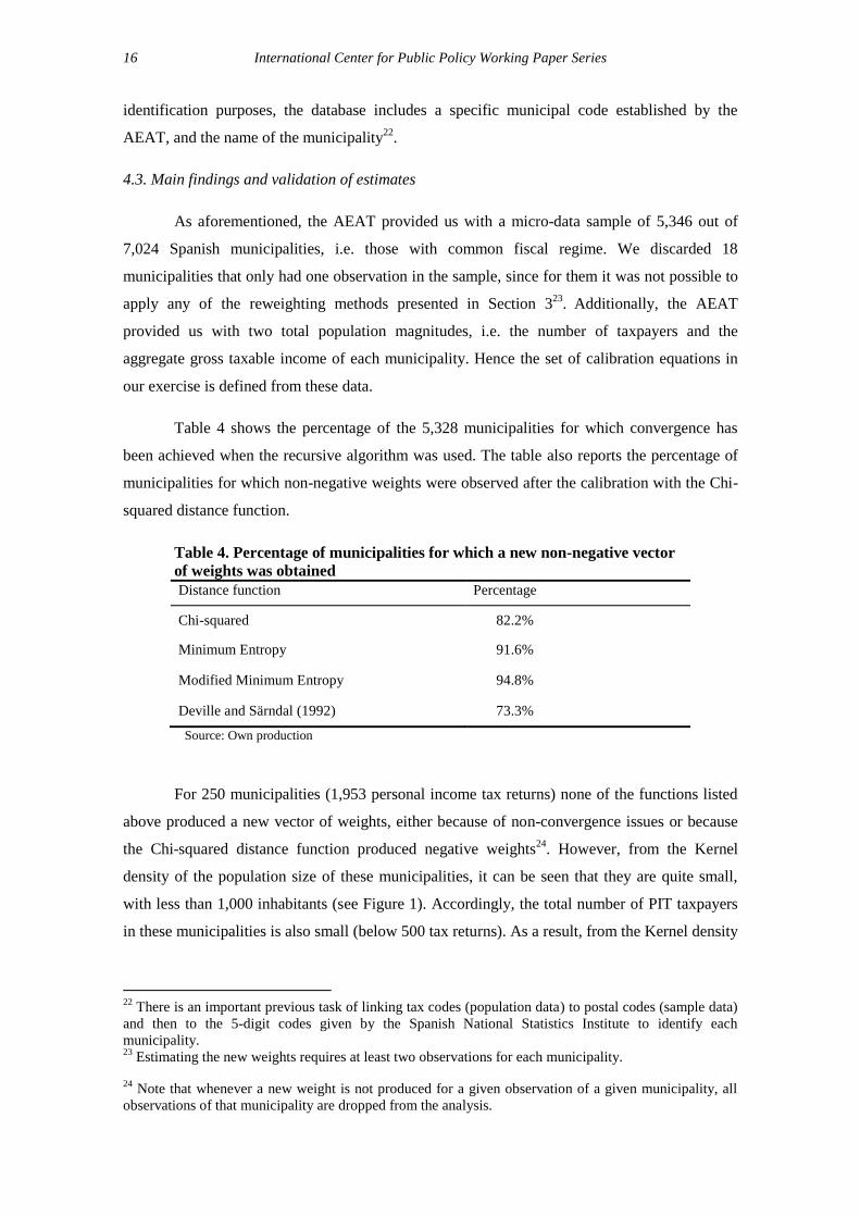
Table 4 shows the percentage of the 5,328 municipalities for which convergence has
been achieved when the recursive algorithm was used. The table also reports the percentage of
municipalities for which non-negative weights were observed after the calibration with the Chi-
squared distance function.
Table 4. Percentage of municipalities for which a new non-negative vector
of weights was obtained
Distance function Percentage
Chi-squared 82.2%
Minimum Entropy 91.6%
Modified Minimum Entropy 94.8%
Deville and Särndal (1992) 73.3%
Source: Own production
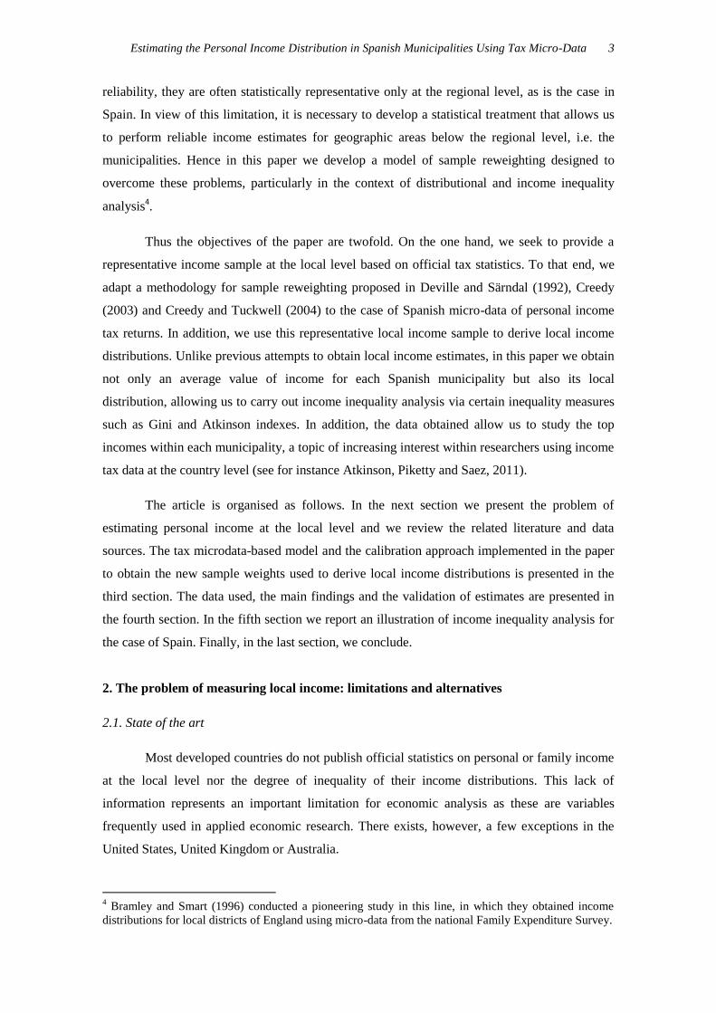
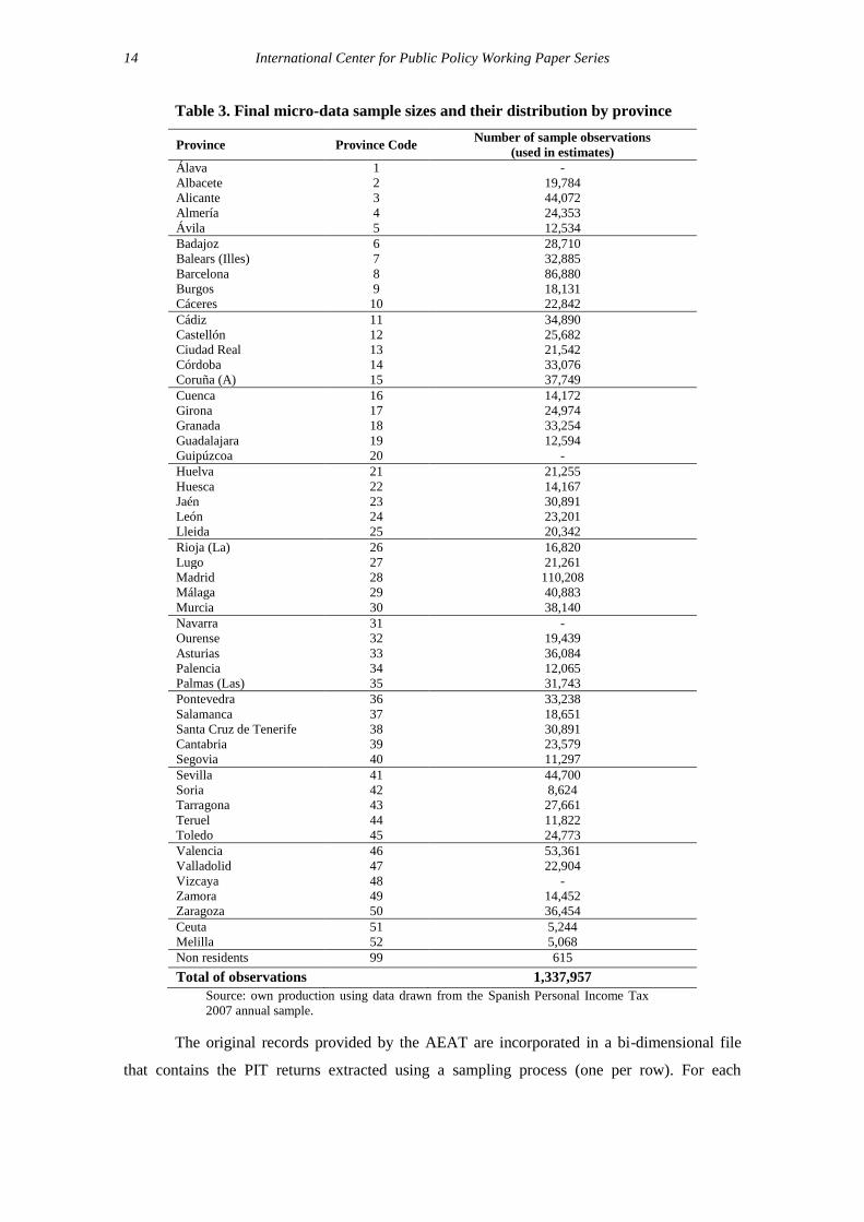
For 250 municipalities (1,953 personal income tax returns) none of the functions listed
above produced a new vector of weights, either because of non-convergence issues or because
the Chi-squared distance function produced negative weights24
. However, from the Kernel
density of the population size of these municipalities, it can be seen that they are quite small,
with less than 1,000 inhabitants (see Figure 1). Accordingly, the total number of PIT taxpayers
in these municipalities is also small (below 500 tax returns). As a result, from the Kernel density
22
There is an important previous task of linking tax codes (population data) to postal codes (sample data)
and then to the 5-digit codes given by the Spanish National Statistics Institute to identify each
municipality. 23
Estimating the new weights requires at least two observations for each municipality. 24
Note that whenever a new weight is not produced for a given observation of a given municipality, all
observations of that municipality are dropped from the analysis.
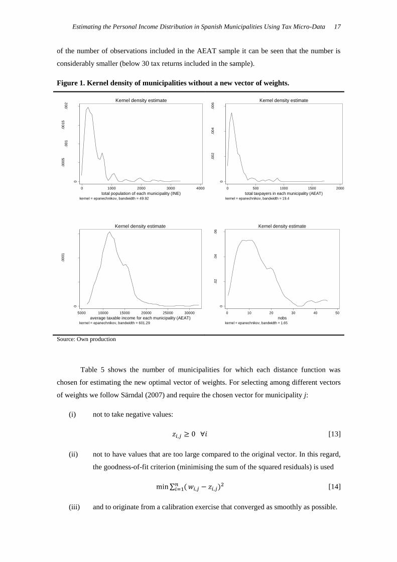
Estimating the Personal Income Distribution in Spanish Municipalities Using Tax Micro-Data 17
of the number of observations included in the AEAT sample it can be seen that the number is
considerably smaller (below 30 tax returns included in the sample).
Figure 1. Kernel density of municipalities without a new vector of weights.
Source: Own production
Table 5 shows the number of municipalities for which each distance function was
chosen for estimating the new optimal vector of weights. For selecting among different vectors
of weights we follow Särndal (2007) and require the chosen vector for municipality j:
(i) not to take negative values:
[13]
(ii) not to have values that are too large compared to the original vector. In this regard,
the goodness-of-fit criterion (minimising the sum of the squared residuals) is used
∑ ( )
[14]
(iii) and to originate from a calibration exercise that converged as smoothly as possible.
0
.00
05
.00
1.0
015
.00
2
De
nsity
0 1000 2000 3000 4000
total population of each municipality (INE)kernel = epanechnikov, bandwidth = 49.92
Kernel density estimate
0
.00
00
5.0
001
.00
01
5
De
nsity
5000 10000 15000 20000 25000 30000
average taxable income for each municipality (AEAT)kernel = epanechnikov, bandwidth = 601.29
Kernel density estimate
0
.00
2.0
04
.00
6
De
nsity
0 500 1000 1500 2000
total taxpayers in each municipality (AEAT)kernel = epanechnikov, bandwidth = 19.4
Kernel density estimate
0
.02
.04
.06
De
nsity
0 10 20 30 40 50
nobskernel = epanechnikov, bandwidth = 1.65
Kernel density estimate
18 International Center for Public Policy Working Paper Series
Table 5. Chosen distance function for each municipality
Distance function Number of municipalities %
Chi-squared 1,607 31.65%
Minimum Entropy 2,496 49.15%
Modified Minimum Entropy 473 9.31%
Deville and Särndal (1972) 502 9.89%
Total: 5,078 100
Source: Own production
As can be seen, the Minimum Entropy distance is the function adopted in most cases,
according to the selection criteria explained above. The Chi-squared and the DS distance
function then follow. However, as Deville and Särndal (1992) prove, all the above-listed
functions generate asymptotically-equivalent calibration estimators. Hence changes of the
distance function will often have only minor effects on the variance of the calibration estimator,
even if the sample size is rather small.
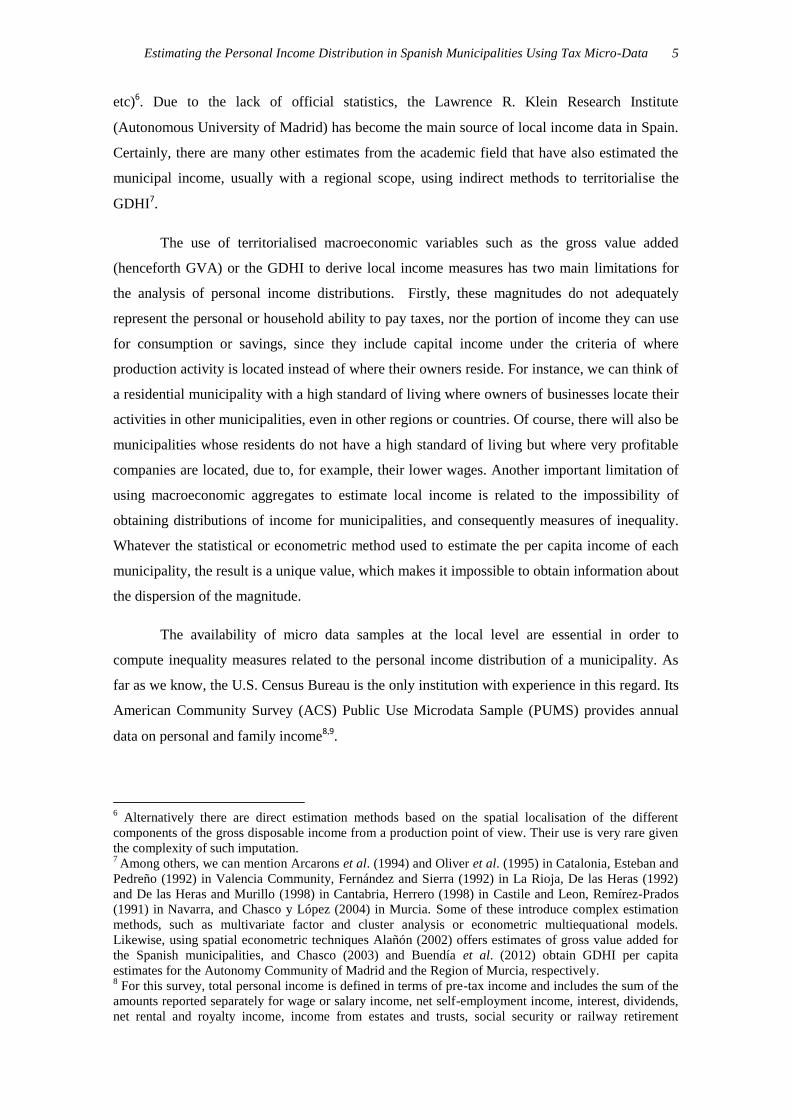
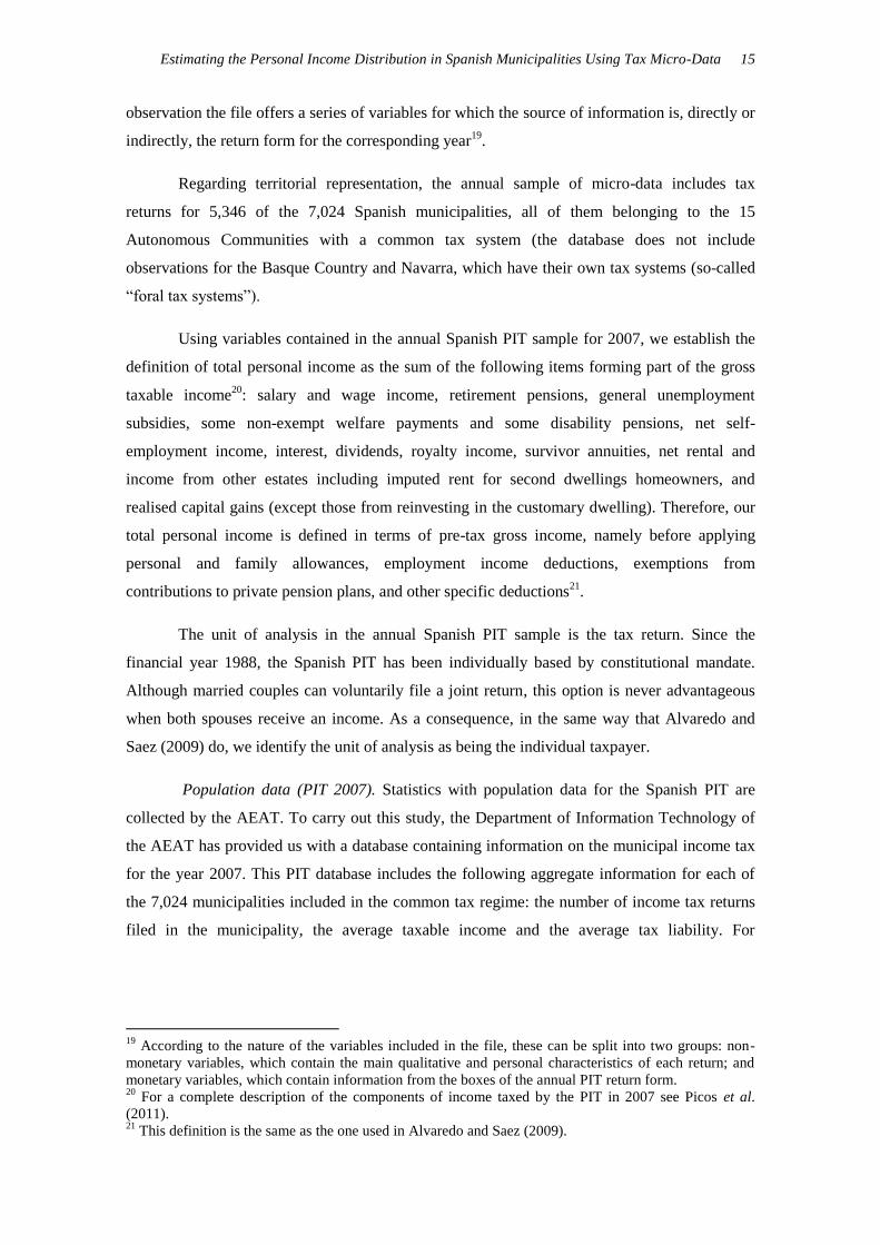
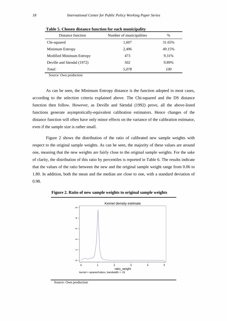
Figure 2 shows the distribution of the ratio of calibrated new sample weights with
respect to the original sample weights. As can be seen, the majority of these values are around
one, meaning that the new weights are fairly close to the original sample weights. For the sake
of clarity, the distribution of this ratio by percentiles is reported in Table 6. The results indicate
that the values of the ratio between the new and the original sample weight range from 0.06 to
1.80. In addition, both the mean and the median are close to one, with a standard deviation of
0.98.
Figure 2. Ratio of new sample weights to original sample weights
Source: Own production
01
23
45
De
nsity
0 1 2 3 4 5
ratio_weightkernel = epanechnikov, bandwidth = .01
Kernel density estimate
Estimating the Personal Income Distribution in Spanish Municipalities Using Tax Micro-Data 19
Table 6. Distribution of the ratio of new to original sample weights.
Percentiles Ratio z/w
1% 0.06013
5% 0.31796
10% 0.62805
25% 0.91277
50% 0.99691
75% 1.04968
90% 1.14317
95% 1.24089
99% 1.80791
Mean 0.97445
St. Dev. 0.98183
Source: Own production
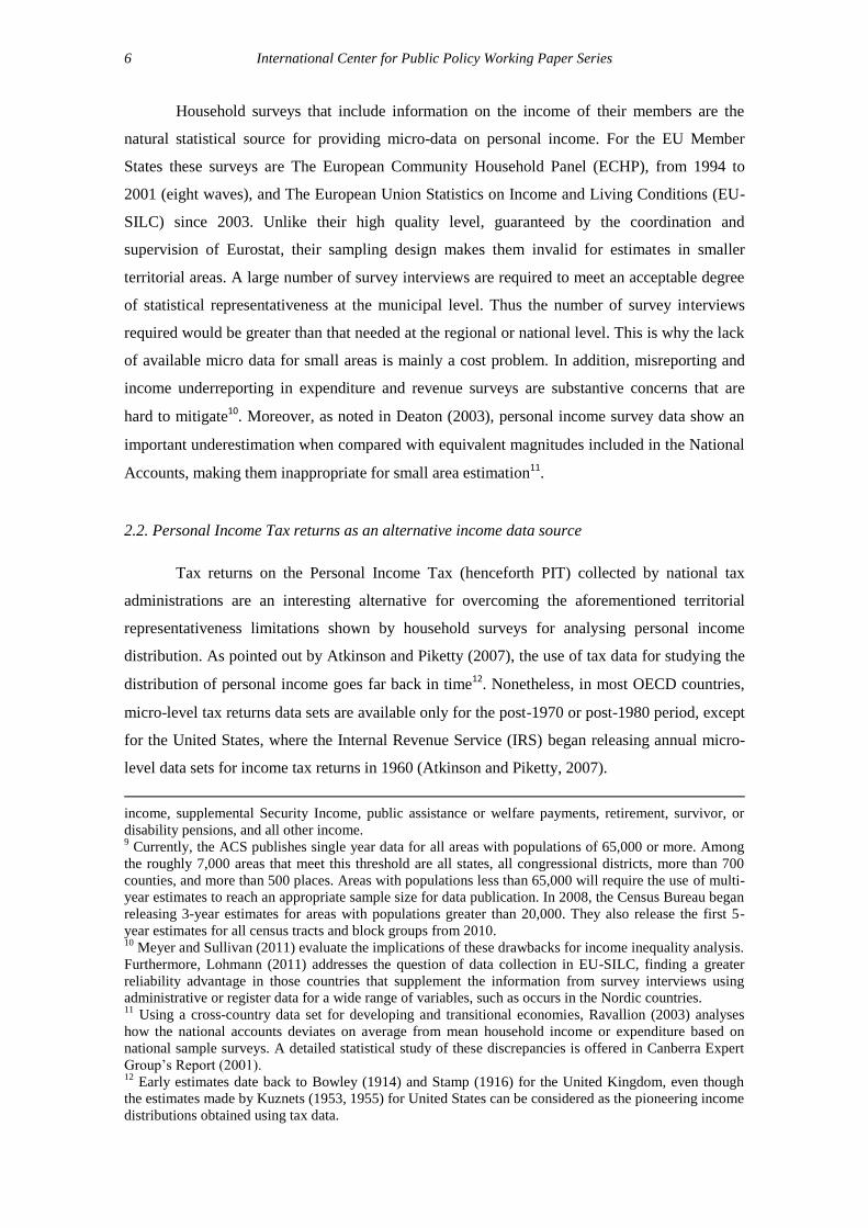
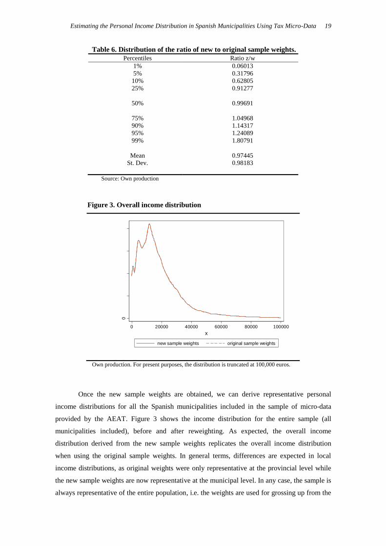
Figure 3. Overall income distribution
Own production. For present purposes, the distribution is truncated at 100,000 euros.
Once the new sample weights are obtained, we can derive representative personal
income distributions for all the Spanish municipalities included in the sample of micro-data
provided by the AEAT. Figure 3 shows the income distribution for the entire sample (all
municipalities included), before and after reweighting. As expected, the overall income
distribution derived from the new sample weights replicates the overall income distribution
when using the original sample weights. In general terms, differences are expected in local
income distributions, as original weights were only representative at the provincial level while
the new sample weights are now representative at the municipal level. In any case, the sample is
always representative of the entire population, i.e. the weights are used for grossing up from the
0
.00
00
1.0
000
2.0
000
3.0
000
4
kd
en
sity t
axa
ble
_ba
se
0 20000 40000 60000 80000 100000
x
new sample weights original sample weights
20 International Center for Public Policy Working Paper Series
sample in order to obtain estimates of population values. As can be seen in Figure 3, estimates
of the income density function for the national total with new and old weights are virtually
identical.
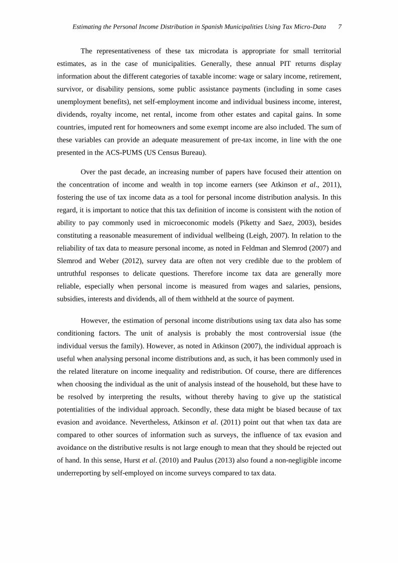
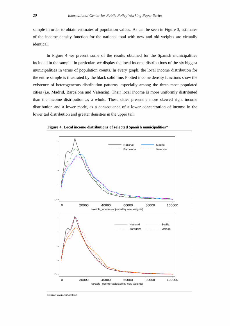
In Figure 4 we present some of the results obtained for the Spanish municipalities
included in the sample. In particular, we display the local income distributions of the six biggest
municipalities in terms of population counts. In every graph, the local income distribution for
the entire sample is illustrated by the black solid line. Plotted income density functions show the
existence of heterogeneous distribution patterns, especially among the three most populated
cities (i.e. Madrid, Barcelona and Valencia). Their local income is more uniformly distributed
than the income distribution as a whole. These cities present a more skewed right income
distribution and a lower mode, as a consequence of a lower concentration of income in the
lower tail distribution and greater densities in the upper tail.
Source: own elaboration
Figure 4. Local income distributions of selected Spanish municipalities*
0
.00
00
1.0
000
2.0
000
3.0
000
4
0 20000 40000 60000 80000 100000
taxable_income (adjusted by new weights)
National Madrid
Barcelona Valencia
0
.00
00
1.0
000
2.0
000
3.0
000
4
0 20000 40000 60000 80000 100000
taxable_income (adjusted by new weights)
National Sevilla
Zaragoza Málaga
Estimating the Personal Income Distribution in Spanish Municipalities Using Tax Micro-Data 21
5. Personal income inequality in Spanish municipalities
The estimated local income distributions obtained in the previous section are a valuable
and informative tool for distributional and income inequality analysis. As an illustration, in this
section we perform an analysis of local inequality for a sample of Spanish municipalities based
on the computation of two of the most common measurements of inequality, the Gini and the
Atkinson indexes. In line with the abovementioned literature on top incomes, we also include
measurements of the top 1%, 0.5% and 0.1% income shares.
The Gini coefficient (Gini, 1912) is probably the standard in the income inequality
literature. This index is defined as the area between the 45° (which indicates perfect equality)
and the Lorenz curve,
( ) ∫ ( )
[15]
where the Lorenz curve of income ( ) at such p-values of ranked relative cumulated-
population (so that, ( )) can be defined mathematically by the expression,
( ) ( ) ∫ ( ) ⁄
[16]
Accordingly, the Gini coefficient takes values between zero (perfect equality) and one
(complete inequality).
The second income inequality measurement used in our analysis is the Atkinson index
(Atkinson, 1970). This index differs from the Gini index in its explicitly ethical foundation. In
fact, the Atkinson index is based upon a social welfare function, including a weighting
parameter ε which measures aversion to inequality, so that the index becomes more sensitive to
changes at the lower end of the income distribution as approaches to 1, while if the level of
inequality aversion falls (i.e. as it approaches 0) the index becomes more sensitive to changes at
the upper end of the income distribution. For the equally distributed equivalent income is
simply the average level of income, while for the Rawlsian criterion is used (i.e. social
welfare function is close to the maximum concavity).
From a continuous approach to the income distribution, the Atkinson index is defined
as,
( ) (∫ (
)
( )
)
[17]
And it values on the interval ranging from 0 (if the income is distributed equally) to 1 (if
the inequality is the highest). In our analysis, we have chosen the parameter values 0.5 and 1.
22 International Center for Public Policy Working Paper Series
As is known, the value 1 provides similar findings to Gini index, while the value 0.5 provides
information for a reduced aversion to inequality.
Using the AEAT micro-data and the new sample weights, we calculate these two
different income inequality measures at the municipality level25
,26
. The results for both income
inequality indexes are reported in Figures 5 and 6, respectively. Detailed results on these
indexes are presented in the Appendix.
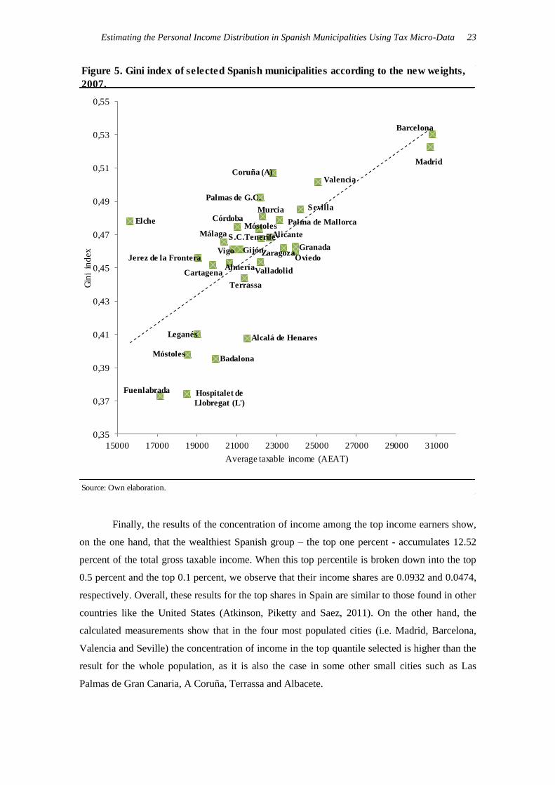
For the purpose of this empirical exercise we have selected a small sample of Spanish
municipalities. In particular, only the results for the 35 most populated municipalities are
reported. Three main finding arise from the results. On the one hand, the Gini coefficient has a
wide range of variation, as it takes values from 0.37 to 0.53. On the other hand, there exists a
clearly positive correlation between the Gini coefficient and the average gross taxable income of
the municipality, with a correlation coefficient of 0.65. This result suggests that richer cities
have more income inequality (more unequal income distributions) than the poorer ones. This
result also holds for the Atkinson coefficients, whose results exhibit a similar pattern of
variation than those presented for the Gini coefficient, even though we find some differences
between cities due to the specific degree of inequality aversion that is behind every measure
calculated. As can be seen in the comparison of Figures 5 and 6, the different degrees of
inequality aversion for the three inequality indices considered provide some changes in the
relative order of cities with an average income below 25,000 euros.
25
There are several plausible alternatives for calculating these expressions when using micro-data. In
particular, we use the Stata’s ineqdeco ado file provided by Jenkins and adapted for our stratified sample
of micro-data. The inequality aversion parameter of the Atkinson index ( ) takes the values 0.5, 1 and 2.
26
Confidence intervals via bootstrap re-sampling methods (Mills and Zandvakili, 1997) have been
calculated for both inequality measures. In particular, two types of bootstrap confidence intervals are
obtained, using respectively the alpha-percentile method and the normal-distribution method. Given the
large size of the micro-data sample used in our analysis, the number of bootstrap replicates has been set at
100. Likewise, we have calculated the standard errors for both inequality indexes. The results show very
low bootstrapped standard errors, an expected result given the very large size of our sample. Nonetheless,
they are available on request from the authors or in Hortas-Rico et al. (2013).
Estimating the Personal Income Distribution in Spanish Municipalities Using Tax Micro-Data 23
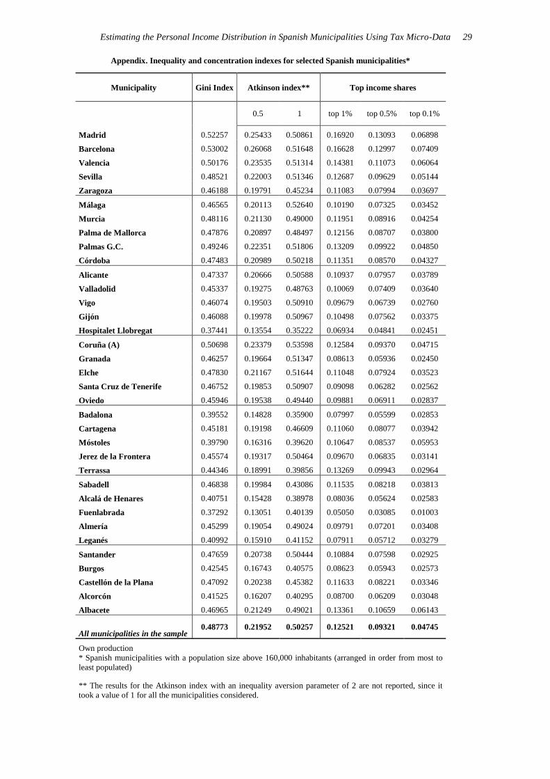
Finally, the results of the concentration of income among the top income earners show,
on the one hand, that the wealthiest Spanish group – the top one percent - accumulates 12.52
percent of the total gross taxable income. When this top percentile is broken down into the top
0.5 percent and the top 0.1 percent, we observe that their income shares are 0.0932 and 0.0474,
respectively. Overall, these results for the top shares in Spain are similar to those found in other
countries like the United States (Atkinson, Piketty and Saez, 2011). On the other hand, the
calculated measurements show that in the four most populated cities (i.e. Madrid, Barcelona,
Valencia and Seville) the concentration of income in the top quantile selected is higher than the
result for the whole population, as it is also the case in some other small cities such as Las
Palmas de Gran Canaria, A Coruña, Terrassa and Albacete.
Source: Own elaboration.
Figure 5. Gini index of selected Spanish municipalities according to the new weights,
2007.
Madrid
Barcelona
Valencia
Sevilla
Zaragoza
Málaga
Murcia
Palma de Mallorca
Palmas de G.C.
Córdoba
Alicante
Valladolid
Vigo Gijón
Hospitalet de
Llobregat (L')
Coruña (A)
Granada
Elche
S.C.Tenerife
Oviedo
Badalona
Cartagena
Móstoles
Jerez de la Frontera
Terrassa
Móstoles
Leganés
Fuenlabrada
Almería
Alcalá de Henares
0,35
0,37
0,39
0,41
0,43
0,45
0,47
0,49
0,51
0,53
0,55
15000 17000 19000 21000 23000 25000 27000 29000 31000
Gin
i in
dex
Average taxable income (AEAT)

24 International Center for Public Policy Working Paper Series
Source: Own elaboration.
Figure 6. Atkinson index of selected Spanish municipalities according to the new weights,
2007.
Madrid
Barcelona
Valencia
Sevilla
ZaragozaMálaga
MurciaPalma de Mallorca
Palmas de G.C.
Córdoba
Alicante
ValladolidVigo
Gijón
Hospitalet de
Llobregat
Coruña (A)
Granada
Elche
Oviedo
Badalona
Cartagena
Móstoles
Jerez de la Frontera
Leganés
Terrassa
Sabadell
Fuenlabrada
Almería
Alcalá de Henares
0,1
0,15
0,2
0,25
0,3
15000 17000 19000 21000 23000 25000 27000 29000 31000
Atk
inso
n in
dex
(ε=
0.5
)
Average taxable income (AEAT)
Madrid
BarcelonaValenciaSevilla
Zaragoza
Málaga
Murcia
Palma de Mallorca
Palmas de G.C.
Córdoba Alicante
Valladolid
Vigo Gijón
Hospitalet de
Llobregat
Coruña (A)
Granada
Elche
Oviedo
Badalona
Cartagena
Móstoles
Jerez de la Frontera
Leganés
Terrassa
Sabadell
Fuenlabrada
Almería
Alcalá de Henares
0,3
0,35
0,4
0,45
0,5
0,55
15000 17000 19000 21000 23000 25000 27000 29000 31000
Atk
inso
n in
dex
(ε=
1)
Average taxable income (AEAT)
Estimating the Personal Income Distribution in Spanish Municipalities Using Tax Micro-Data 25
6. Concluding remarks
Local income data are a key economic indicator, widely used in applied economic
research. Despite its importance, there is a lack of official data on personal incomes for
territorial areas smaller than the provinces or regions. This paper makes use of official data on
personal income tax returns and a reweighting procedure to derive a representative income
sample at the local level. The methodology implemented here relies on the calibration approach
proposed in Deville and Särndal (1992), Creedy (2003) and Creedy and Tuckwell (2004) for
survey reweighting. In doing so, we adjust the original micro-data sample weights in order to
make them representative at the local level, given that our estimates would now face smaller
spatial areas used as a strata sample extraction.
Unlike previous attempts in the literature to acquire local income estimates, the results
obtained allow us to derive not only an average value of income but its local distribution, a
valuable and informative tool for income inequality analysis. We apply this methodology to
Spanish micro-data and illustrate its potential use in income inequality analysis. The results
suggest remarkable relationships between some variables of interest, such as the level of income
in the municipalities, their inequality, the concentration of top incomes and their population
size, among others. Nonetheless, a further analysis of those relationships lies beyond the scope
of this paper and, as such, should be addressed in future research.
Overall, the methodology presented here represents a starting point for income
inequality analysis at the local level. A wide range of potential implementations arise from these
results. The illustration presented here could be extended to the whole set of municipalities, in
order to get a picture of income inequality within municipalities in Spain. In addition, the recent
availability of PIT annual samples for several years would allow us to perform both cross-
section and longitudinal income inequality analyses for Spanish municipalities. Also note that
the present paper has focused on pre-tax income, but its extension to after-tax income would
allow us to undertake redistributive analysis in order to evaluate the impact of personal income
tax in municipalities. Likewise, the data provided here would allow us to deeply investigate the
behaviour of top incomes by municipality, complementing existing research literature on this
topic. Lastly, we would like to clarify that the only purpose of these findings is to provide an
illustration of the possibilities for applied economic analysis offered by the implemented
methodology. We think the availability of representative information on the income level of
Spanish municipalities and its distribution opens up a fruitful area of research in many topics of
urban economics and local public finance.
26 International Center for Public Policy Working Paper Series
References
Alvaredo, F. and Saez, E. (2009). “Income and wealth concentration in Spain from a historical
and fiscal perspective”, Journal of the European Economic Association, 7 (5): 1140-
1167.
Atkinson, A. B. (1970). “On the measurement of inequality”, Journal of Economic Theory, 2:
244-263.
Atkinson, A. B. (2007). “Measuring Top Incomes: Methodological Issues”, en A. B. Atkinson
and T. Piketty (eds.), Top Incomes over the Twentieth Century. Oxford, UK: Oxford
University Press, Ch. 2, pp. 18-42.
Atkinson, A. B. and T. Piketty (2007). Top Incomes over the Twentieth Century. Oxford, UK:
Oxford University Press.
Atkinson, A. B., T. Piketty and E. Saez (2011). “Top Incomes in the Long Run of History”,
Journal of Economic Literature, 49 (1): 3-71.
Bowley, A. L. (1914). “The British Super-Tax and the Distribution of Income”, Quarterly
Journal of Economics, 28: 255–68.
Bramley, G. and Smart, G. (1996). “Modelling local income distributions in Britain”, Regional
Studies, 30 (3): 239-255.Creedy, J. (2003). “Survey reweighting for tax microsimulation
modelling”. New Zealand Treasury Working Paper Series, 17/03.
Buendía, J. D., Esteban, M. and J. C. Sánchez de la Vega (2012). "Estimación de la renta bruta
disponible municipal mediante técnicas de econometría espacial: Un ejercicio de
aplicación", Revista de Estudios Regionales, (93): 119-142.
Canberra Expert Group on Household Income Statistics (2001). Final Report and
Recommendations. Ottawa: Canberra Expert Group on Household Income Statistics.
Chasco, C. (2003). Econometría espacial aplicada a la predicción-extrapolación de datos
microterritoriales. Consejería de Economía e Innovación tecnológica de la Comunidad de
Madrid.
Chasco, C. and F. López (2004). “Modelos de regresión espacio-temporales en la estimación de
la renta municipal: el caso de la región de Murcia, Estudios de Economía Aplicada, 22-
3:1-24
Creedy, J. and Tuckwell, I. (2004). "Reweighting household surveys for tax microsimulation
modelling: An application to the New Zealand household economic survey", Australian
Journal of Labour Economics 7 (1), 71–88.
Deaton, A. (2003). “Household Surveys, Consumption, and the Measurement of Poverty”,
Economic Systems Research, 15 (2): 135-159.
Deville, J. and Särndal, C. (1992) Calibration estimators in survey sampling. Journal of the
American Statistical Association, 87: 376–382.
Elbers, C., Lanjouw, J. and Lanjouw, P. (2003). “Micro-level estimation of poverty and
inequality”, Econometrica, 71 (1): 355–364.
Gini, C. (1912) “Variabilità e mutabilità, contributo allo studio delle distribuzioni e relazioni
statistiche”, Studi Economico-Giuridici dell’ Universiti di Cagliari, 3, (2): 1-158.
Estimating the Personal Income Distribution in Spanish Municipalities Using Tax Micro-Data 27
Haslett, S., Jones, G., Noble, A. and Ballas, D. (2010). “More of Less? Comparing small area
estimation, spatial microsimulation, and mass imputation”, JSM 2010 Proceedings of the
Section on Survey Research Methods, Alexandria, VA: American Statistical Association:
1584-1598.
Haughton, J. H. and Khandker, S. R. (2009). Handbook on poverty and inequality. Washington
DC: The World Bank.
Hortas-Rico, M; Onrubia, J.; Pacifico, D. (2013) Personal income distribution at the local level.
An estimation for Spanish municipalities using tax micro-data. International Center for
Public Policy Working Paper Series, paper 1314, International Center for Public Policy,
Andrew Young School of Policy Studies, Georgia State University.
Hurst, E., Li, G., and Pugsley, B. 2010. “Are Household Surveys like Tax Forms: Evidence
from Income Underreporting of the Self Employed,” NBER Working Paper, no.16527.
Kovar, J.G. and Whitridge, P.J. (1995). “Imputation of Business Survey Data,” in Cox, B.G.,
Binder, D.A., Chinnappa, B.N., Christianson, A., Colledge, M.J., Kott, P.S. (eds.),
Business Survey Methods. New York: John Wiley and Sons. pp. 403-423.
Kuznets, S. (1953). Shares of Upper Income Groups in Income and Savings. National Bureau of
Economic Research, New York.
Kuznets, S. (1955). “Economic growth and income inequality”, American Economic Review,
65: 1-28.
Lambert, P. J. (2001). The distribution and redistribution of Income, 3rd
edition. Manchester:
Manchester University Press.
Leigh, A. (2007). “How Closely Do Top Income Shares Track Other Measures of Inequality?,
The Economic Journal, 117 (524): F619-F633.
Lohmann, H. (2011). “Comparability of EU-SILC survey and register data: The relationship
among employment, earnings and poverty”, Journal of European Social Policy, 21 (1): 1-
18.
Meyer, B. and Sullivan, J. X. (2011). “Viewpoint: Further Results on Measuring the Well-Being
of the Poor using Income and Consumption”, Canadian Journal of Economics, 44 (1):
52-87
Mills J. A and Zandvakili, A. (1997). “Statistical inference via bootstrapping for measures of
inequality”, Journal of Applied Econometrics, 12: 133-150.
Paulus, A. (2011). “Tax Evasion and Measurement Error: A Comparison of Survey Income with
Tax Records”, paper presented at 69th Congress of the International Institute of Public
Finance, Taormina, Italy, 22-25 August 2013.
Picos, F. (2006). “Microsimulación mediante fusión de Phogue y Panel de Declarantes para
evaluar reformas fiscales”. Revista de Economía Aplicada, 41: 33-60.
Picos, F., Pérez, C. and González, M. C. (2011). “La muestra de declarantes de IRPF de 2007:
descripción general y principales magnitudes”, Documentos de Trabajo del Instituto de
Estudios Fiscales, 01/11.
Piketty, T. and Saez, E. (2003). “Income inequality in the United States, 1913–1998”, The
Quarterly Journal of Economics, 118 (1): 1-41.
28 International Center for Public Policy Working Paper Series
Rahman, A., Harding, A., Tanton, R. and Liu, S. (2010). “Methodological Issues in Spatial
Microsimulation Modelling for Small Area Estimation”, International Journal of
Microsimulation, 3 (2): 3-22.
Rao, J.N.K. (1999). “Some recent advances in model-based small area estimation”, Survey
Methodology, 25: 175–186.
Rao, J.N.K. (2003). Small Area Estimation. New York: Wiley.
Ravallion, M. (2003). “Measuring aggregate welfare in developing countries: how well do
national accounts and surveys agree?”, Review of Economics and Statistics, 85 (3): 645-
652.
Remírez-Prados, J. A. (1991). Una estimación de la renta familiar disponible a nivel municipal.
El caso de Navarra. Madrid: Confederación Española de Cajas de Ahorro.
Särndal, C. (2007). The calibration approach in survey theory and practice. Survey
Methodology, 33 (2): 99–119.
Slemrod, J. and Weber, C. (2012). “Evidence of the invisible: toward a credibility revolution in
the empirical analysis of tax evasion and the informal economy”, International Tax and
Public Finance, 19 (1): 25-53.
Stamp, J. C., Lord (1914). “A New Illustration of Pareto’s Law”, Journal of the Royal
Statistical Society, 77: 200–4.
Stamp, J. C., Lord (1916). British Incomes and Property. London: P. S. King.
Tanton, R. and Edwards, K. (eds.)(2013). Spatial Microsimulation: A Reference Guide for
Users. Dordrecht: Springer
Estimating the Personal Income Distribution in Spanish Municipalities Using Tax Micro-Data 29
Appendix. Inequality and concentration indexes for selected Spanish municipalities*
Municipality Gini Index Atkinson index** Top income shares
0.5 1 top 1% top 0.5% top 0.1%
Madrid 0.52257 0.25433 0.50861 0.16920 0.13093 0.06898
Barcelona 0.53002 0.26068 0.51648 0.16628 0.12997 0.07409
Valencia 0.50176 0.23535 0.51314 0.14381 0.11073 0.06064
Sevilla 0.48521 0.22003 0.51346 0.12687 0.09629 0.05144
Zaragoza 0.46188 0.19791 0.45234 0.11083 0.07994 0.03697
Málaga 0.46565 0.20113 0.52640 0.10190 0.07325 0.03452
Murcia 0.48116 0.21130 0.49000 0.11951 0.08916 0.04254
Palma de Mallorca 0.47876 0.20897 0.48497 0.12156 0.08707 0.03800
Palmas G.C. 0.49246 0.22351 0.51806 0.13209 0.09922 0.04850
Córdoba 0.47483 0.20989 0.50218 0.11351 0.08570 0.04327
Alicante 0.47337 0.20666 0.50588 0.10937 0.07957 0.03789
Valladolid 0.45337 0.19275 0.48763 0.10069 0.07409 0.03640
Vigo 0.46074 0.19503 0.50910 0.09679 0.06739 0.02760
Gijón 0.46088 0.19978 0.50967 0.10498 0.07562 0.03375
Hospitalet Llobregat 0.37441 0.13554 0.35222 0.06934 0.04841 0.02451
Coruña (A) 0.50698 0.23379 0.53598 0.12584 0.09370 0.04715
Granada 0.46257 0.19664 0.51347 0.08613 0.05936 0.02450
Elche 0.47830 0.21167 0.51644 0.11048 0.07924 0.03523
Santa Cruz de Tenerife 0.46752 0.19853 0.50907 0.09098 0.06282 0.02562
Oviedo 0.45946 0.19538 0.49440 0.09881 0.06911 0.02837
Badalona 0.39552 0.14828 0.35900 0.07997 0.05599 0.02853
Cartagena 0.45181 0.19198 0.46609 0.11060 0.08077 0.03942
Móstoles 0.39790 0.16316 0.39620 0.10647 0.08537 0.05953
Jerez de la Frontera 0.45574 0.19317 0.50464 0.09670 0.06835 0.03141
Terrassa 0.44346 0.18991 0.39856 0.13269 0.09943 0.02964
Sabadell 0.46838 0.19984 0.43086 0.11535 0.08218 0.03813
Alcalá de Henares 0.40751 0.15428 0.38978 0.08036 0.05624 0.02583
Fuenlabrada 0.37292 0.13051 0.40139 0.05050 0.03085 0.01003
Almería 0.45299 0.19054 0.49024 0.09791 0.07201 0.03408
Leganés 0.40992 0.15910 0.41152 0.07911 0.05712 0.03279
Santander 0.47659 0.20738 0.50444 0.10884 0.07598 0.02925
Burgos 0.42545 0.16743 0.40575 0.08623 0.05943 0.02573
Castellón de la Plana 0.47092 0.20238 0.45382 0.11633 0.08221 0.03346
Alcorcón 0.41525 0.16207 0.40295 0.08700 0.06209 0.03048
Albacete 0.46965 0.21249 0.49021 0.13361 0.10659 0.06143
All municipalities in the sample 0.48773 0.21952 0.50257 0.12521 0.09321 0.04745
Own production
* Spanish municipalities with a population size above 160,000 inhabitants (arranged in order from most to
least populated)
** The results for the Atkinson index with an inequality aversion parameter of 2 are not reported, since it
took a value of 1 for all the municipalities considered.