The threshold effect of exchange rate volatility on FDI determinant …euroasiapub.org/wp-content/uploads/2016/09/5FMMAY-… · · 2017-08-04IJRFM Volume 5, Issue 5 (May, 2015)

IJRFM Volume 5, Issue 5 (May, 2015) (ISSN 2231-5985) International Journal of Research in Finance and Marketing (IMPACT FACTOR – 5.230)

International Journal of Research in Finance & Marketing Email id: [email protected] http://www.euroasiapub.org

48

The threshold effect of exchange rate volatility on FDI

determinant nexus – A panel smooth transition regression

approach

Po-Chin Wu

Professor,

Department of International Business,

Chung Yuan Christian University, Taiwan

Chia-Jui Chang

Ph.D. candidate,

College of Business, Chung Yuan Christian University,Taiwan

Abstract

This paper adopts a panel smooth transition model ( PSTR) with lagged exchange rate risk

( exchange rate volatility) as the transition variable to estimate the nonlinear process of

China’s FDI inflows and the threshold effect of exchange rate risk on the FDI inflows.

Empirically, we use the data set of China’s top ten FDI investment countries during 2000Q1 –

2011Q4. Empirical results show that China’s FDI inflows displays a nonlinear process,

depending on exchange rate risk in different regimes. China’s FDI inflows are nonlinearly

affected by GDP, exchange rate, openness and trade-weighted distance. If government’s

intervention policy or quantitative easing policy is to lead global currencies depreciation for

improving a country’s terms of trade, the related stable of RMB exchange rate will

continuously attract FDI inflow to China.

Keyword: panel smooth transition regression model, exchange rate volatility, nonlinearity,

quantitative easing

JEL classification numbers:F63, O11,C32,F21



49

1. Introduction

With the global economic growth, foreign direct investment (FDI) has become an important

issue to a country’s economic growth.Governments take proper policies to attract FDI inflow

for improving countries’economic or social welfare (Subasat and Bellos, 2011; Sun, 2011).

The United Nations Conference on Trade and Development (UNCTAD), (2011) indicates that

theglobal FDI growth was over six times from 1990 to 2010. In 2013, the emerging market

and developing countries have attracted FDI inflows over 50% global FDI inflows. In fact, FDI

have significant contributions to the debt repayments, export and foreign exchange revenue,

especially of the developing countries or transition economies (Daly and Zhang, 2010).

During the last 10 years, China’s economic growth has attracted the sight around the

world.According to the statistics of UNCTAD, China’s FDI inflows reached 124 billion US

dollars from 2010 to 2011 and wasthe second large FDI recipient country (Tang, Selvanathan

and Selvanathan, 2008). Thus, what factors drive the rapid growth of China’s FDI inflows has

been a crucial issue to be noticed by researchers (Lau and Bruton, 2008; Agrawal, 2011).

Many previous studies (see for example,Kojima, 1973; Dunning, 1980) suggested that

firms’overseas investment not only originates from their specific technology or monopoly

advantage, but also reflectthe change of their domestic economic conditions. Thus, FDI

inflow can be considered as the behavior for transition economies to seek benefit and

decrease risk. To the end, some the currency authorities may use intervention policies to

reduce exchange rate volatility for promoting export expansion, FDI and trade balance

accumulation (Hsiao, Pan, and Wu, 2011). In recent ten years, China’s exchange rate of

China’s currency is in a stable position;therefore, the increase in FDI resource country of

exchange rate volatility would lead to a higher foreign production risk (Zhang, 2008). That is

the increase of China’s FDI inflows can be regarded as foreign capitals are seeking more

stable production cost and eliminating uncertainty.

Previousresearches on FDI supported that China has attracted global FDI inflow by its rich

resource, labor productivity and government incentivessince the economy reform in

1979.The determinants that affect FDI include wage, exchange rate, political risk and

economic growth. (Vijayakumar, Sridharan and Rao, 2010; Gast and Herrmann, 2008; Aw and

Tang, 2010; Edwards, 1990; Tang, Selvanathan and Selvanathan, 2008; Agrawal, 2011;Rani

and Dhanda, 2011).However, the variables they used are ad hoc (Deardoff, 1995) andlake of

theoretical basis; therefore, the collinearity among variables is easy ignored (Resmini, 2000).

In addition, many researchers adopt different approaches to estimate the determinants of



50

FDI.For instance, linear regression with structural breaks, log linear regression model,

multiple regression analysis, panel data or gravity panel data model (Boyrie, 2009; Azam and

Lukman, 2010; Shahmoradi, Thimmaiah and Indumati, 2010; Aw and Tang, 2010; Wang, Wei

and Liu, 2010; Subasat and Bellos, 2011). However, these approaches can only identify the

determinants of FDI based on single a country, and ignore the problems of small sample size

and heterogeneity.Although panel data models can resolve non-stationarityand

heterogeneity problems (Hsiao, 2006), they still cannot capture the nonlinearity of variable

under investigation.Many nonlinear modelare developed, such as the Markov switching

(MS)model, threshold autoregression(TAR)model and neural network (NN) model.However,

these methods are limited to their extreme regime switching or unclear economic

meanings.Thus, it is necessary to adopt proper model to estimate nonlinear FDI

behavior.Empirically, the panel smooth transition regression (PSTR) model can capture the

nonlinear characteristic of FDI and threshold effect of exchange raterisk on FDI. Hence,

PSTR model is a proper model for this paper to study the nonlinear path of FDI.

In sum, this paper contributes to the existing literature in three distinctive ways. First, we

adopt the PSTR model to estimate the determinants of FDI and identify the nonlinear regime

switching effect of FDI inflows. Second, we endogenously estimate the best lagged transition

variable to capture its time lag effect on FDI inflows. Third, using economic theory to

determineregressorsinfluencing FDI inflows for avoiding random selection of explanatory

variables.

The rest of this paper is organized as follows. Section 2 briefly introduces the PSTR model

and the specification of our modified gravity model on FDI inflows. Section 3 brings the

procedures for estimating the modified PSTR model. Section 4 shows the data and empirical

results. The final section concludes the paper.

2. The Model

2.1 PSTR model

To estimate the determinants of FDI, we must simultaneously resolve theheterogeneous and

time-varying problems. Following González, et al. (2005), the model can be written as

follows:

' '

, 0 , 1 , , ,( ; , )i t i i t i t i t i ty x x G z c (1)

wherei=1,…,N, and t=1,…,T. N and T denote the cross-section and time dimensions of the

panel, respectively. yi,tis a dependent variable and xi,t is a K-dimensional vector of



51

time-varying independent variable. μiis the fixed individual effect.G(Zi,t;γ,c) is the transition

function bounded between 0 and 1 and dependent on the transition variable Zi,t, which can

be an exogenous variable or a combination of the lagged endogenous one (van Dijk,

Terasvirta, &Franses, 2002). γ is the transition or slope parameter.c is the threshold or

location parameter. γ and c are endogenouslyestimated. εi,tis a residual.Follows González et

al. (2005), a transition function (Eq.(2)) can be used to describe the nonlinear and smooth

switching process. For m=1, the function can be described as a logistic specification with a

single monotonic transition of the coefficients from 0 to ( 0 1 ) as ,i tz increases. For

m=2, the transition function has its minimum at 1 2( ) / 2c c where the transition function

can be specified as an exponential function (Eq. (3)).

1

, ,1( ; , ) 1 exp( ( ))

m

i t i t jjG z c z c

(2)

wherem denotesthe number of thresholds or location parameters, γ>0 and c1≤c2≤c3≤…≤cm. A

higher γ means the transition of the dependent variable becomes rougher and transition

function tends towards the indicator functionG(Zi,t;γ,c) (=1, if Zi,t ≥c; =0, otherwise). PSTR

model switch to PTR model when γ→∞;contrarily, when γ→0, the model becomes a panel

with fixed effects. From an empirical aspect, González et al. (2005) suggest that it is sufficient

to consider only the cases of m=1 or m=2 to capture the nonlinear process of variable under

investigation.

2.2 Modified gravity model of FDI

Original gravity model suggests that the determinants of FDI inflow are the market sizes and

distance between source and host countries.Mátyás (1997) arguesthat a complete gravity

model should includetime effect, fixed effect and export effect. However, since China’s

economy reform in 1992, the time effect is insufficient.For an open economy, thecapital of

FDI inflow could be treated as the excess supply of foreign exchange market and is related to

import and export (Fleming, 1962; Mundell, 1963 ); therefore, FDI canbe the function of

price, exchange rate, income (output) and interest rate.

In sum, this paper consider the FDI inflows as a function of relative income,relative CPI

differential, relative exchange rate, openness, relative interest differential, trade-weighted

distance and transition variable (current or lagged exchange rate volatility).



52

, 1 , 2 , 3 , 4 , 5 , 6 , ,i t i i t i t i t i t i t i t i tFDI RI RCPI RREE OPEN IRD TDIS

, 1 , 2 , 3 , 4 , 5 , 6 ,i t i i t i t i t i t i t i tFDI GDP CPI ER OP ID TD

(3)

1 2 3 4 5 6

' ' ' ' ' '

, , , , , ,1( )

r

i t i t i t i t i t i tiGDP CPI ER OP ID TD

,( ; , )i t dG ERV c ,i t

(4)

where t and i denote time dimensions and FDI source country;FDIi,t denotes ratio of FDI

inflows of country i to China’s GDP;CPIi,t denotes price differential between country i and

China;RREEi,tis the real effective exchange rate of China to country i;Openi,tdenotes China’s

trade openness;IRDi,t is the interest rate differential between China and source country i,

and TDISi,tstands for the trade-weighted distance to describe trade which is not only affected

by fixed geographic distance but also varied by time and trade volume. Following González et

al. (2005), PSTR can be written as Eq.(4) where ERVi,t-d, d=1,2,3,4,5 denotes the lagged

exchange rate volatility, μi denotes a fixed individual effect andεi,t is a residual term.

The transition variable exchange rate volatility, could be treated as the proxy of risk to

capture the pulsate in foreign market exchange (Axel, Inessa and Alexei, 2014) and varies

across individuals and with time. G(ERVi,t-d;γ,c) is the transition function to describe the

smooth transition process of FDI. Compared to the function provided by González et al.

(2005), we use a lagged transition variable instead of current transition variable implying

that exchange rate risk has a lagged effect on FDI. The marginal effect of regressor on FDI is

measured byθk+θk(ERVi,t-d;γ,c)

Our PSTR model is different to the model suggested by González et al. (2005) and the

following researchers (Jude, 2010; Ibarra and Trupkin, 2011; Seleteng, Bittencourt and van

Eyden, 2013) in three distinctive aspects. First, the panael data used in this paper is china’s

top ten investment source countries. Second, the transition variable adopted is a d-period

lagged exchange rate risk to capture its lagged effects on FDI. Third, the optimal length is

determined by the AIC and BIC statistics.

3. Estimation and specification test

To estimate thePSTR model, we must first to test the linearity under PSTR model.If the

nonlinearity is accepted, we determine the number of optimal transition functions by

performingthe no remaining non-linearity test. Finally, we apply nonlinear least squares to



53

estimate individual effects of PSTR model.

3.1 Choice of transition variable

In a PSTR model, the effects of regressors on the dependent variable are influenced by the

number of transition functions and the transition variable. This paper adopts exchange rate

volatility as the transition variable, which is highly related with a country’s monetary policy.

According to the risk averse theory, the increase in exchange rate volatility would deter FDI

inflows (Goldberg and Kolstad , 1995). China’s currency authority can use intervention policy

to reduce exchange rate volatility for promoting export and trade balance (Hsiao, Pan, and

Wu, 2011). In addition, the impact of exchange rate volatility on FDI may take some time;

therefore, we use lagged exchange rate volatility as the transition variable.

3.2 Linearity and no remaining nonlinearity tests

FollowingFouquau, Hurlin, and Rabaud (2008), the linearity test is performed under the null

hypothesis: H0:γ=0 or H’0 :β=0. Replacing transition function G(ERVi,t-d;γi,ci) with its first-order

Taylor expansions aroundγ=0 and let γ=1, we then obtain the flowing auxiliary equation:

, 1 , 2 , 3 , 4 , 5 , 6 ,i t i i t i t i t i t i t i tFDI RI RCPI RREE OPEN IRD TDIS

' ' '

1 , , 2 , , 3 , ,i t i t d i t i t d i t i t dRI ERV RCPI ERV RREE ERV

' ' '

4 , , 5 , , 6 , , ,i t i t d i t i t d i t i t d i tOPEN ERV IRD ERV TDIS ERV (5)

whered=0,1,2,3,4,5to allow the current and lagged exchange rate volatility in transition

function. The linearity test is conducted under the null hypothesis

' ' ' ' ' '

0 1 2 3 4 5 6H ：.If SSR0denotes panel sum of squared residuals under

linear model and SSR1 denotes panel sum of squared residuals under PSTR model with single

threshold, the corresponding LM-statistic can be calculated by Eq.(6).

0 1 0[( ) / ] / [ / ( )]FLM SSR SSR K SSR TN N K (6)

whereK denotes the number of predictor variables.Under null hypothesis,LMF statistic has

an asymptotic χ2(K) distribution.

4. Empirical results

4.1 Data description

This paper adopts China’s top ten FDI source countries during 20001Q-20114Q. These

countries include Hong Kong, Taiwan, Japan, Singapore, US, Korea, UK, Germany, French and



54

Netherlands, and their FDI in China account for 92.76% of total foreign investment in China.

Data set comes from National Bureau of Statistics of China.

To confirm the effectiveness of estimation results in the PSTR model, we need to execute the

stationary analysis. Following Baltagi (2008), we adopt unit root test and cointegration

analysis to investigate whether the series is stationary. Levin, Lin, and Chu, (2002) indicates

that LLC test performs well when N lies between 5 and 250 and T lies between 5 and 250.

The data set includes 10 countries (N=10) and 48 quarters (T=48); hence we use the LLC test

to perform the stationarity test.

4.2 Empirical results

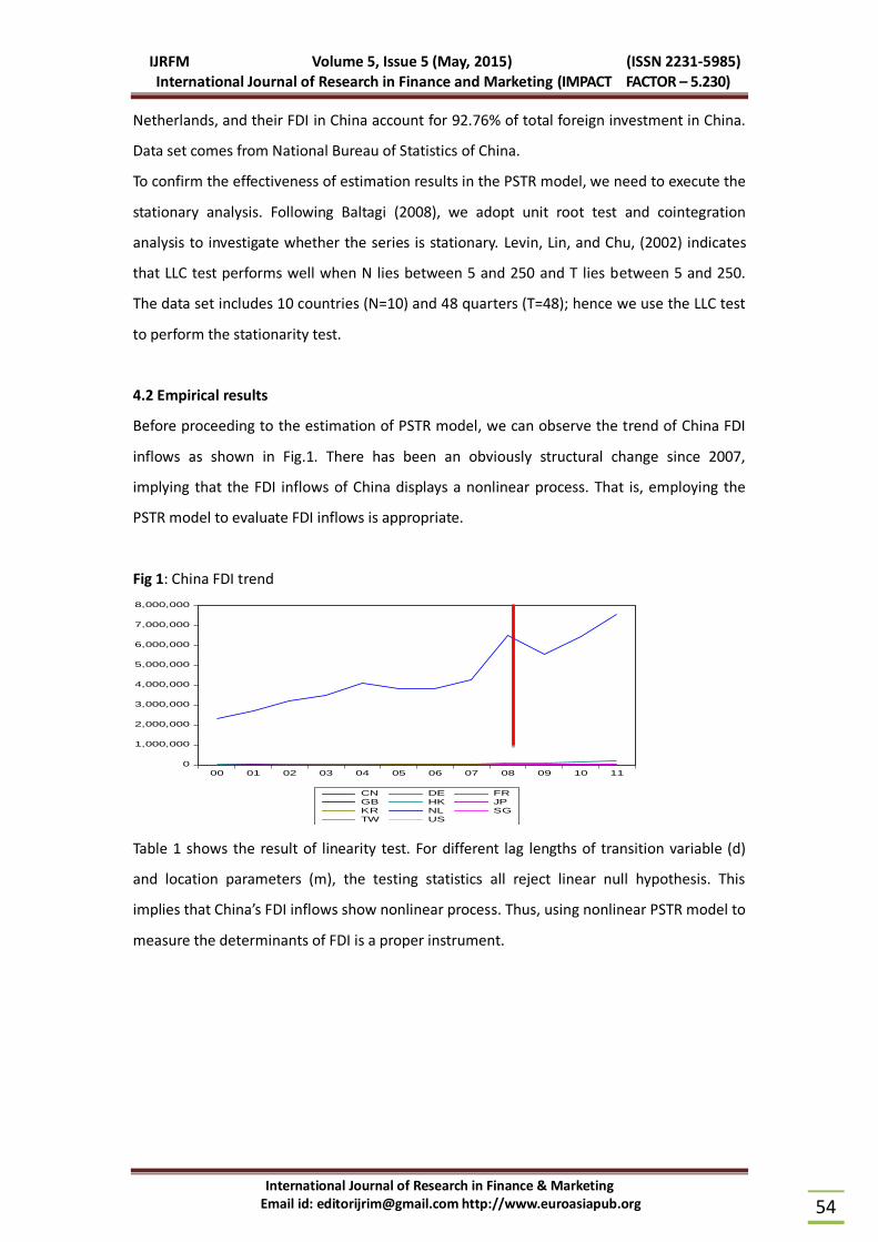
Before proceeding to the estimation of PSTR model, we can observe the trend of China FDI

inflows as shown in Fig.1. There has been an obviously structural change since 2007,

implying that the FDI inflows of China displays a nonlinear process. That is, employing the

PSTR model to evaluate FDI inflows is appropriate.

Fig 1: China FDI trend

Table 1 shows the result of linearity test. For different lag lengths of transition variable (d)

and location parameters (m), the testing statistics all reject linear null hypothesis. This

implies that China’s FDI inflows show nonlinear process. Thus, using nonlinear PSTR model to

measure the determinants of FDI is a proper instrument.

0

1,000,000

2,000,000

3,000,000

4,000,000

5,000,000

6,000,000

7,000,000

8,000,000

00 01 02 03 04 05 06 07 08 09 10 11

CN DE FRGB HK JP

KR NL SG

TW US



55

Table 1: Linearity test

Lag length of transition variable Testing statistic Location parameters (m)

ERVi,t-d m=1 m=2

LM 25.519 [0.000] 50.314 [0.000]

d=0 LMF 4.342 [0.000] 4.469 [0.000]

LRT 26.222 [0.000] 53.151 [0.000]

LM 22.009 [0.001] 50.445 [0.000]

d=1 LMF 3.718 [0.001] 4.489 [0.000]

LRT 22.553 [0.000] 53.363 [0.000]

LM 49.659 [0.000] 44.105 [0.000]

d=2 LMF 8.939 [0.000] 3.871 [0.000]

LRT 52.483 [0.000] 46.365 [0.000]

LM 55.660 [0.000] 59.116 [0.000]

d=3 LMF 10.210 [0.000] 5.394 [0.000]

LRT 59.415 [0.000] 63.376 [0.000]

LM 23.021 [0.000] 45.970 [0.000]

d=4 LMF 3.901 [0.000] 4.064 [0.000]

LRT 23.645 [0.000] 48.552 [0.000]

LM 48.002 [0.000] 49.101 [0.000]

d=5 LMF 8.671 [0.000] 4.383 [0.000]

LRT 50.899 [0.000] 52.138 [0.000]

Notes: The transition variable in the PSTR model is the (lagged) Exchange rate volatility,

ERVi,t-d, d=0,1,2,…,5. The digits in brackets are the p-values. H0:linear model against H1:PSTR

model with at least one threshold variable. LM, LMF, and LRT denote the statistics of the

Wald test, Fisher test, and likelihood ratio test, respectively.

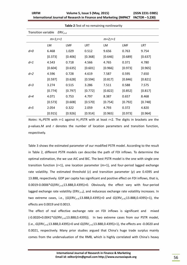
Once, the linearity test is executed, we can proceed to the no remaining nonlinear test. Table

2 shows the test results. Evidently, in all situations, the testing statistics cannot significantly

reject the null hypothesis that the PSTR model has at least on transition function. That is, the

optimal PSTR model has only one transition function (i.e.,γ=1 ).



56

Table 2:Test of no remaining nonlinearity

Transition variable ERVi,t-d

m=1;r=1 m=2;r=1

LM LMF LRT LM LMF LRT

d=0 6.468

[0.373]

1.029

[0.406]

0.512

[0.368]

9.656

[0.646]

0.763

[0.689]

9.754

[0.637]

d=1 4.543

[0.604]

0.718

[0.635]

4.566

[0.601]

4.765

[0.966]

0.371

[0.973]

4.780

[0.965]

d=2 4.596

[0.597]

0.728

[0.628]

4.619

[0.594]

7.587

[0.817]

0.595

[0.846]

7.650

[0.821]

d=3 3.274

[0.774]

0.515

[0.797]

3.286

[0.772]

7.511

[0.822]

0.588

[0.852]

7.575

[0.817]

d=4 4.071

[0.573]

0.753

[0.608]

4.797

[0.570]

8.387

[0.754]

0.657

[0.792]

8.468

[0.748]

d=5 2.054

[0.915]

0.322

[0.926]

2.059

[0.914]

4.793

[0.965]

0.372

[0.973]

4.820

[0.964]

Notes: H0:PSTR with r=1 against H1:PSTR with at least r=2. The digits in brackets are the

p-values.M and r denotes the number of location parameters and transition function,

respectively.

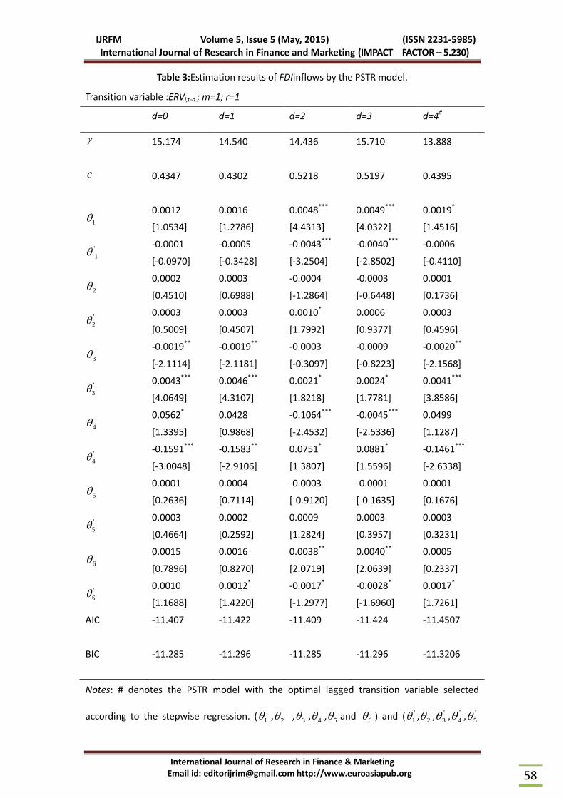
Table 3 shows the estimated parameter of our modified PSTR model. According to the result

in Table 2, different PSTR models can describe the path of FDI inflows. To determine the

optimal estimation, the we use AIC and BIC. The best PSTR model is the one with single one

transition function (r=1), one location parameter (m=1), and four-period lagged exchange

rate volatility. The estimated threshold (c) and transition parameter (γ) are 0.4395 and

13.888, respectively. GDP per capita has significant and positive effect on FDI inflows, that is,

0.0019-0.0006*G(ERVi,t-4;13.888,0.4395)>0. Obviously, the effect vary with four-period

lagged exchange rate volatility (ERVi,t-4), and reducesas exchange rate volatility increases. In

two extreme cases, i.e., (G(ERVi,t-4;13.888,0.4395)=0 and G(ERVi,t-4;13.888,0.4395)=1), the

effects are 0.0019 and 0.0013.

The effect of real effective exchange rate on FDI inflows is significant and mixed

(-0.0020+0.0041*G(ERVi,t-4;13.888,0.4395)). In two extreme cases from our PSTR model,

(i.e., G(ERVi,t-4;13.888,0.4395)=0 and G(ERVi,t-4;13.888,0.4395)=1), the effects are -0.0020 and

0.0021, respectively. Many prior studies argued that China's huge trade surplus mainly

comes from the undervaluation of the RMB, which is highly correlated with China's heavy



57

intervention in the foreign exchange market. However, with the rapid change of world

economy, RMB becomes more stable, which induces FDI inflows from other countries to

China to avoid risk from domestic market. That I, a higher exchange rate volatility is

beneficial for China to attract foreign investment. Regarding the impact of openness on FDI,

we obtain a ambiguous result, i.e., (0.0499-0.1461*G(ERVi,t-4;13.888,0.4395)). In two extreme

cases from our model, (ERVi,t-4;13.888,0.4395)=0 and G(ERVi,t-4;13.888,0.4395)=1), the

effects are 0.0499 and -0.0964, respectively. The reason maybe that when exchange rate

volatility is over the threshold, China’s economic growth is faster or slower than those of

import and export through J curve effect; therefore, the positive or negative effect would

depend on which effect is more larger. If exchange rate volatility is higher than the threshold,

openness can induce more foreign capital entering China.

As to the trade-weighted distance, it has a significant effect on China’s FDI inflows, which is

different from the result populated by previous linear model. The probable reason is that

higher investment of sample countries leads to higher import-export volume, which reduces

the negative impact of distance on FDI inflows. In two extreme cases,

(G(ERVi,t-4;13.888,0.4395)=0 and G(ERVi,t-4;13.888,0.4395)=1), the effects are 0.0005 and

0.0075, respectively. Obviously, when exchange rate volatility is over the threshold, the

positive effect of trade-weighed distance on FDI inflows would increase. Moreover, relative

CPI and interest rate differential have insignificant effect, implying that foreign investors do

not care about the change of price factor and investment cost, since China has a

environment of lower price and capital cost (Arnold, 2012) .

If we replace four-period lagged exchange rate volatility with its current value, the

estimation result is biased. For example, in two extreme cases from the model,

(G(ERVi,t-4;13.888,0.4395)=0 and G(ERVi,t-4;13.888,0.4395)=1), the effects of relative GDP on

FDI are 0.0012 and 0.0011, respectively. Under the situation of using four-period lagged

exchange rate volatility as the transition variable, the effects are 0.0019 and 0.0013.

In sum, under the situation of a higher exchange rate volatility, relative GDP per capita

reduces the positive effect on FDI inflow into China; real effective exchange rate will deter

FDI inflows. The degree of trade openness has similar effect to the relative effective

exchange rate through J-curve effect. Trade distance variable still shows positive effect to

promote FDI inflows but with higher fluctuation will be less negative effect. That is, to attract

foreign capital enter into China through improving the states of regressors, the authority of

China will face a trade-off.



58

Table 3:Estimation results of FDIinflows by the PSTR model.

Transition variable :ERVi,t-d ; m=1; r=1

d=0 d=1 d=2 d=3 d=4#

15.174 14.540 14.436 15.710 13.888

c 0.4347 0.4302 0.5218 0.5197 0.4395

1 0.0012

[1.0534]

0.0016

[1.2786]

0.0048***

[4.4313]

0.0049***

[4.0322]

0.0019*

[1.4516]

'

1 -0.0001

[-0.0970]

-0.0005

[-0.3428]

-0.0043***

[-3.2504]

-0.0040***

[-2.8502]

-0.0006

[-0.4110]

2 0.0002

[0.4510]

0.0003

[0.6988]

-0.0004

[-1.2864]

-0.0003

[-0.6448]

0.0001

[0.1736]

'

2 0.0003

[0.5009]

0.0003

[0.4507]

0.0010*

[1.7992]

0.0006

[0.9377]

0.0003

[0.4596]

3 -0.0019**

[-2.1114]

-0.0019**

[-2.1181]

-0.0003

[-0.3097]

-0.0009

[-0.8223]

-0.0020**

[-2.1568]

'

3 0.0043***

[4.0649]

0.0046***

[4.3107]

0.0021*

[1.8218]

0.0024*

[1.7781]

0.0041***

[3.8586]

4 0.0562*

[1.3395]

0.0428

[0.9868]

-0.1064***

[-2.4532]

-0.0045***

[-2.5336]

0.0499

[1.1287]

'

4 -0.1591***

[-3.0048]

-0.1583**

[-2.9106]

0.0751*

[1.3807]

0.0881*

[1.5596]

-0.1461***

[-2.6338]

5 0.0001

[0.2636]

0.0004

[0.7114]

-0.0003

[-0.9120]

-0.0001

[-0.1635]

0.0001

[0.1676]

'

5 0.0003

[0.4664]

0.0002

[0.2592]

0.0009

[1.2824]

0.0003

[0.3957]

0.0003

[0.3231]

6 0.0015

[0.7896]

0.0016

[0.8270]

0.0038**

[2.0719]

0.0040**

[2.0639]

0.0005

[0.2337]

'

6 0.0010

[1.1688]

0.0012*

[1.4220]

-0.0017*

[-1.2977]

-0.0028*

[-1.6960]

0.0017*

[1.7261]

AIC -11.407 -11.422 -11.409 -11.424 -11.4507

BIC -11.285 -11.296 -11.285 -11.296 -11.3206

Notes: # denotes the PSTR model with the optimal lagged transition variable selected

according to the stepwise regression. ( 1 , 2 , 3 , 4 , 5 and 6 ) and ( '

1 , '

2 , '

3 , '

4 , '

5



59

and '

6 ) are the estimated coefficients of the relative GDP per capita, relative CPI, relative

exchange rate, openness, relative interest rate difference and trade-weighted distance, in

regime 1 and 2, respectively. The digits in brackets are the t-statistics.

5. Conclusion.

This paper constructs a FDI inflows model as the PSTR framework to evaluate whether

China’s FDI inflows are nonlinear and the threshold effect of exchange rate volatility on the

inflows. Empirical results can be summed up as follows. First, China’s FDI inflows from main

countries display a nonlinear process. Second, relative exchange rate volatility has a

nonlinear effect on FDI inflows through the determinants in four periods later. Third, the

speed of FDI inflow in 2006-2010 is higher than that before 2006, this result cannot be

identified under linear model. If china tries to promote GDP growth and increase foreign

exchange reserves, enlarging exchange rate volatility is a useful method for China to attract

foreign capital. In practice, regional risk can enlarge the relative exchange rate volatility

which will push FDI inflow and increase China’s foreign reserve.

Our results suggest that: (1) Expanding FDI inflows can increase China’s GDP. (2) Keeping

lower exchange rate volatility through intervention can promote FDI inflow; (3) Reducing

restrictions can drive international trade and FDI inflows.

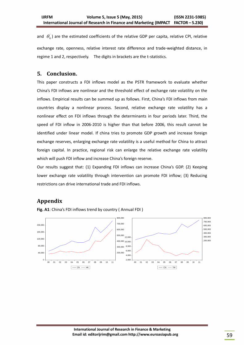
Appendix

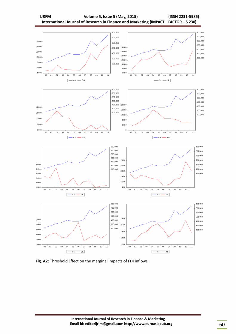
Fig. A1: China’s FDI inflows trend by country ( Annual FDI )

0

40,000

80,000

120,000

160,000

200,000

200,000

300,000

400,000

500,000

600,000

700,000

800,000

00 01 02 03 04 05 06 07 08 09 10 11

CN HK

2,000

4,000

6,000

8,000

10,000

12,000

200,000

300,000

400,000

500,000

600,000

700,000

800,000

00 01 02 03 04 05 06 07 08 09 10 11

CN TW



60

Fig. A2: Threshold Effect on the marginal impacts of FDI inflows.

4,000

6,000

8,000

10,000

12,000

14,000

16,000

200,000

300,000

400,000

500,000

600,000

700,000

800,000

00 01 02 03 04 05 06 07 08 09 10 11

CN SG

6,000

8,000

10,000

12,000

14,000

16,000

18,000

200,000

300,000

400,000

500,000

600,000

700,000

800,000

00 01 02 03 04 05 06 07 08 09 10 11

CN JP

6,000

8,000

10,000

12,000

14,000

200,000

300,000

400,000

500,000

600,000

700,000

800,000

00 01 02 03 04 05 06 07 08 09 10 11

CN US

0

4,000

8,000

12,000

16,000

20,000

200,000

300,000

400,000

500,000

600,000

700,000

800,000

00 01 02 03 04 05 06 07 08 09 10 11

CN KR

1,600

2,000

2,400

2,800

3,200

3,600

200,000

300,000

400,000

500,000

600,000

700,000

800,000

00 01 02 03 04 05 06 07 08 09 10 11

CN UK

800

1,200

1,600

2,000

2,400

2,800

200,000

300,000

400,000

500,000

600,000

700,000

800,000

00 01 02 03 04 05 06 07 08 09 10 11

CN FR

1,000

2,000

3,000

4,000

5,000

6,000

200,000

300,000

400,000

500,000

600,000

700,000

800,000

00 01 02 03 04 05 06 07 08 09 10 11

CN DE

1,200

1,600

2,000

2,400

2,800

200,000

300,000

400,000

500,000

600,000

700,000

800,000

00 01 02 03 04 05 06 07 08 09 10 11

CN NL



61

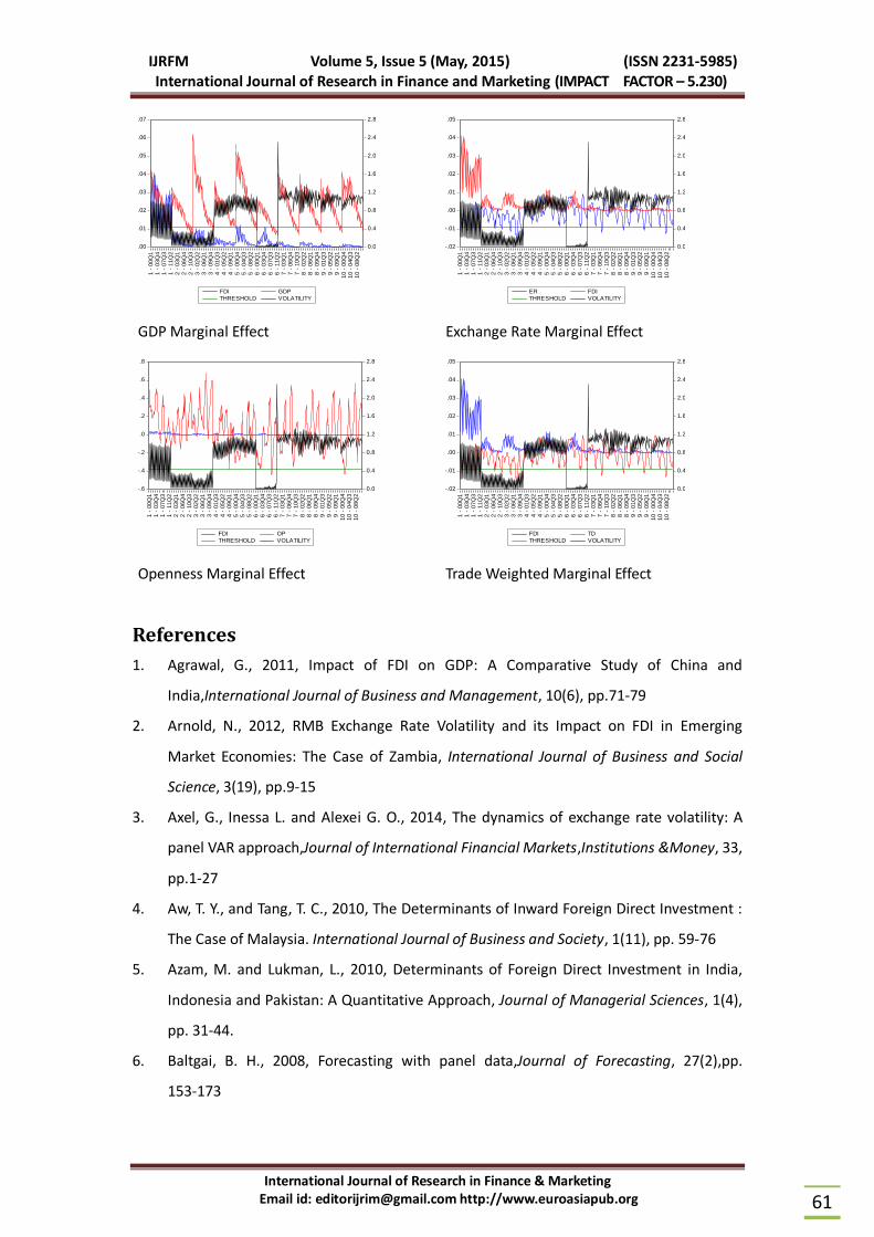
GDP Marginal Effect Exchange Rate Marginal Effect

Openness Marginal Effect Trade Weighted Marginal Effect

References

1. Agrawal, G., 2011, Impact of FDI on GDP: A Comparative Study of China and

India,International Journal of Business and Management, 10(6), pp.71-79

2. Arnold, N., 2012, RMB Exchange Rate Volatility and its Impact on FDI in Emerging

Market Economies: The Case of Zambia, International Journal of Business and Social

Science, 3(19), pp.9-15

3. Axel, G., Inessa L. and Alexei G. O., 2014, The dynamics of exchange rate volatility: A

panel VAR approach,Journal of International Financial Markets,Institutions &Money, 33,

pp.1-27

4. Aw, T. Y., and Tang, T. C., 2010, The Determinants of Inward Foreign Direct Investment :

The Case of Malaysia. International Journal of Business and Society, 1(11), pp. 59-76

5. Azam, M. and Lukman, L., 2010, Determinants of Foreign Direct Investment in India,

Indonesia and Pakistan: A Quantitative Approach, Journal of Managerial Sciences, 1(4),

pp. 31-44.

6. Baltgai, B. H., 2008, Forecasting with panel data,Journal of Forecasting, 27(2),pp.

153-173

.00

.01

.02

.03

.04

.05

.06

.07

0.0

0.4

0.8

1.2

1.6

2.0

2.4

2.8

1 -

00Q

1 1

- 0

3Q

4 1

- 0

7Q

3 1

- 1

1Q

2 2

- 0

3Q

1 2

- 0

6Q

4 2

- 1

0Q

3 3

- 0

2Q

2 3

- 0

6Q

1 3

- 0

9Q

4 4

- 0

1Q

3 4

- 0

5Q

2 4

- 0

9Q

1 5

- 0

0Q

4 5

- 0

4Q

3 5

- 0

8Q

2 6

- 0

0Q

1 6

- 0

3Q

4 6

- 0

7Q

3 6

- 1

1Q

2 7

- 0

3Q

1 7

- 0

6Q

4 7

- 1

0Q

3 8

- 0

2Q

2 8

- 0

6Q

1 8

- 0

9Q

4 9

- 0

1Q

3 9

- 0

5Q

2 9

- 0

9Q

1 1

0 -

00

Q4

10

- 0

4Q

3 1

0 -

08

Q2

FDI GDPTHRESHOLD VOLATILITY

-.02

-.01

.00

.01

.02

.03

.04

.05

0.0

0.4

0.8

1.2

1.6

2.0

2.4

2.8

1 -

00Q

1 1

- 0

3Q

4 1

- 0

7Q

3 1

- 1

1Q

2 2

- 0

3Q

1 2

- 0

6Q

4 2

- 1

0Q

3 3

- 0

2Q

2 3

- 0

6Q

1 3

- 0

9Q

4 4

- 0

1Q

3 4

- 0

5Q

2 4

- 0

9Q

1 5

- 0

0Q

4 5

- 0

4Q

3 5

- 0

8Q

2 6

- 0

0Q

1 6

- 0

3Q

4 6

- 0

7Q

3 6

- 1

1Q

2 7

- 0

3Q

1 7

- 0

6Q

4 7

- 1

0Q

3 8

- 0

2Q

2 8

- 0

6Q

1 8

- 0

9Q

4 9

- 0

1Q

3 9

- 0

5Q

2 9

- 0

9Q

1 1

0 -

00

Q4

10

- 0

4Q

3 1

0 -

08

Q2

ER FDITHRESHOLD VOLATILITY

-.6

-.4

-.2

.0

.2

.4

.6

.8

0.0

0.4

0.8

1.2

1.6

2.0

2.4

2.8

1 -

00Q

1 1

- 0

3Q

4 1

- 0

7Q

3 1

- 1

1Q

2 2

- 0

3Q

1 2

- 0

6Q

4 2

- 1

0Q

3 3

- 0

2Q

2 3

- 0

6Q

1 3

- 0

9Q

4 4

- 0

1Q

3 4

- 0

5Q

2 4

- 0

9Q

1 5

- 0

0Q

4 5

- 0

4Q

3 5

- 0

8Q

2 6

- 0

0Q

1 6

- 0

3Q

4 6

- 0

7Q

3 6

- 1

1Q

2 7

- 0

3Q

1 7

- 0

6Q

4 7

- 1

0Q

3 8

- 0

2Q

2 8

- 0

6Q

1 8

- 0

9Q

4 9

- 0

1Q

3 9

- 0

5Q

2 9

- 0

9Q

1 1

0 -

00

Q4

10

- 0

4Q

3 1

0 -

08

Q2

FDI OPTHRESHOLD VOLATILITY

-.02

-.01

.00

.01

.02

.03

.04

.05

0.0

0.4

0.8

1.2

1.6

2.0

2.4

2.8

1 -

00Q

1 1

- 0

3Q

4 1

- 0

7Q

3 1

- 1

1Q

2 2

- 0

3Q

1 2

- 0

6Q

4 2

- 1

0Q

3 3

- 0

2Q

2 3

- 0

6Q

1 3

- 0

9Q

4 4

- 0

1Q

3 4

- 0

5Q

2 4

- 0

9Q

1 5

- 0

0Q

4 5

- 0

4Q

3 5

- 0

8Q

2 6

- 0

0Q

1 6

- 0

3Q

4 6

- 0

7Q

3 6

- 1

1Q

2 7

- 0

3Q

1 7

- 0

6Q

4 7

- 1

0Q

3 8

- 0

2Q

2 8

- 0

6Q

1 8

- 0

9Q

4 9

- 0

1Q

3 9

- 0

5Q

2 9

- 0

9Q

1 1

0 -

00

Q4

10

- 0

4Q

3 1

0 -

08

Q2

FDI TDTHRESHOLD VOLATILITY



62

7. Boyrie, M. E., 2010, Structural Changes, Causality, and Foreign Direct Investments:

Evidence from the Asian Crises of 1997, Global Economy Journal, 4(9), pp. 1-40

8. Daly, K. and Zhang, X., 2010, The Determinants of Foreign Direct Investment in China.

Journal of International Finance and Economics. 3(10), pp. 123-129.

9. Deardoff, A.,1995, Determinants of bilateral trade: does gravity work in a neo-classical

works ? NBER Working paper. 5377.

10. Dunning, J. H., 1980, Toward an Eclectic Theory of International Production : Some

Empirical Test,Journal of International Business Studies, 11(1), pp. 9-31

11. Edwards, S., 1990, Capital flows, foreign direct investment, and debt-equity swaps in

developing countries, NBER working paper no. 3497.

12. Fleming, J. M., 1962, Domestic Financial Policies under Fixed and Floating Exchange

Rates,IMF Staff Papers, 9, pp. 369-379.

13. Fouquau, J., Hurlin, C. and Rabaud, I., 2008, The Feldstein–Horioka puzzle: A panel

smooth transition regression approach,Economic Modeling, 25,pp. 284–299.

14. Gast, M. and Herrmann, R., 2008, Determinants of foreign direct investment of OECD

countries 1991–2001,International Economic Journal, 4(22). Pp. 509–524

15. Goldberg, L.S. and Kolstad C.D., 1995, Foreign Direct Investment , Exchange Rate

Variability and Demand Uncertainty. International Economic Review, 36, pp. 855-873.

16. González, A., Teräsvirta, T. and van Dijk, D., 2005, Panel smooth transition regression

models. Sidney Quantitative Finance Research Centre, Research paper, 165.

17. Hsiao, C., 2006, Panel Data Analysis – Advantages and Challenges. IEPR working paper,

06.49.

18. Hsiao Y. M., Pan, S. C. and Wu. P. C., 2011, Does the central bank's intervention benefit

trade balance? Empirical evidence from China,International Review of Economics and

Finance, 21. Pp. 130–139

19. Ibarra, R. and Trupkin, D., 2011, The relationship between inflation and growth: A panel

smooth transition regression approach for developed and developing countries, BCU

No. 006-2011.

20. Jude, E.C., 2010, Financial Development and Growth : A Panel Smooth Regression

Approach. Journal Of Economic Development, 15(35), pp. 15-34

21. Kojima, K., 1973, A Macroeconomic Approach to Foreign Direct Investment.

Hitotsubashi Journal of Economic, 14, pp. 1-21.

22. Lau, C. M. and Bruton, G. D., 2008, FDI in China : What We Know and What We need to



63

Study Next. Academy of Management Perspectives, Nov., pp. 30-44.

23. Levin, A., Lin, F. and Chu, C., 2002, Unit root tests in panel data: Asymptotic and

finite-sample properties,Journal of Econometrics, 108, pp. 1–24

24. Mátyás, L., 1997, Proper Econometric Specification of the Gravity Model,The World

Economy, 20, pp. 363–368.

25. Mundell, R. A., 1963, Capital Mobility and Stabilization Policy under Fixed and Flexible

Exchange Rates,Canadian Journal of Economics and Political Science, 29, pp. 475-485.

26. Rani, N. and Dhanda, N., 2011, Foreign Direct Investment and Foreign Trade: Evidence

From India, International Journal of Research in Finance & Marketing, 1(3), pp. 67-89.

27. Resmini, L., 2000, The determinants of foreign direct investment into the CEECs : new

evidence from sectoral patterns,Economics of Transition, 8,pp. 665-689.

28. Wang, C., Wei, Y. and Liu, X., 2010, Determinants of Bilateral Trade Flows in OECD

Countries: Evidence from Gravity Panel Data Models,The World Economy, pp. 894-915

29. Shahmoradi, B., Thimmaiah, N. and Indumati, S., 2010, Determinants Of FDI Inflows In

High Income Countries: An Intertemporal And Cross Sectional Analysis Since

1990,International Business & Economics Research Journal, 5(9), pp. 59-64

30. Seleteng, M., Bittencourt, M. and van Eyden R., 2013, Non-linearities in

inflation–growth nexus in the SADC region: A panel smooth transition regression

approach. Economic Modelling, 30(C),pp. 149-156

31. Subasat, T. and Bellos, S., 2011, Economic Freedom and Foreign Direct Investment in

Latin America: A Panel Gravity Model Approach,Economics Bulletin, 3(31), pp.

2053-2065.

32. Sun, H., 2011, Co-Integration Study of Relationship between Foreign Direct Investment

and Economic Growth. International Business Research, 4(4), pp. 226-230.

33. Tang, T.,Selvanathan E. A., and Selvanathan, S. (2008), Foreign Direct Investment,

Domestic Investment and Economic Growth in China: A Time series Analysis,The World

Economy, 31(10), pp. 1292-1309.

34. UNCTAD, (2011),World Investment Report 2011, Non-Equity Modes of International

Production and Development.

35. Vijayakumar, N., Sridharan, P.and Rao, K. C. S., 2010, Determinants of FDI in BRICS

Countries: A panel analysis. Int. Journal of Business Science and Applied Management,

3(5), pp. 1-14.

36. vanDijk, D., Terasvirta, T. and Franses, P. H., 2002, Smooth transition autoregressive

http://econpapers.repec.org/article/eeeecmode/



64

models — a survey of recent developments. Econometric Reviews, 21, pp. 1–47.

37. Wu, P. C., Liu, S. Y. and Pan S. C., 2013, Nonlinear bilateral trade balance-fundamentals

nexus: A panel smooth transition regression approach. International Review of

Economics and Finance, 27, pp.318-329

38. Zhang, H. K., 2008, What attracts Foreign Multinational Corporations to China.

Contemporary Economic Policy, 19(3), pp. 336-348

Documents

The threshold effect of exchange rate volatility on FDI determinant …euroasiapub.org/wp-content/uploads/2016/09/5FMMAY-… · · 2017-08-04IJRFM Volume 5, Issue 5 (May, 2015)