an important determinant of growth. In general, FDI does

Author

Copy

Trade, Foreign Direct Investment, andGrowth: Evidence from TransitionEconomies

HIRANYA K. NATH

Department of Economics and International Business, Sam Houston State University,Huntsville, TX 77341-2118, USA. E-mail: [email protected]

Using a fixed effects panel data approach, this paper empirically examines the

effects of trade and foreign direct investment (FDI) on growth of per capita real GDP

in 13 transition economies of Central and Eastern Europe, and the Baltic region from

1991 to 2005. A significant positive effect of trade on growth is a robust result for

transition economies of this region. In addition, domestic investment appears to be

an important determinant of growth. In general, FDI does not have any significant

impact on growth in these transition economies. However, when we control for the

effects of domestic investment and trade on FDI, it appears to be a significant

determinant of growth for the period after 1995.

Comparative Economic Studies (2009) 51, 20–50. doi:10.1057/ces.2008.20

Keywords: transition economies, trade, FDI, growth, fixed effects panel data

model

JEL Classifications: F14, F21, O52, P33

INTRODUCTION

The experiences of economic transition from a centrally planned to a market-based system in Central and Eastern Europe (CEE) and the former SovietUnion raise two pertinent questions. First, what triggered growth that endedthe ‘transition recession’ experienced by these transition economies inthe early 1990s? Second, what would sustain growth in subsequent periods?This paper is primarily concerned with the second question and examinesthe role of trade and foreign direct investment (FDI) in growth in 13transition economies of Central and Eastern Europe, and the Baltic Region

Comparative Economic Studies, 2009, 51, (20–50)r 2009 ACES. All rights reserved. 0888-7233/09

www.palgrave-journals.com/ces/

Author

Copy

(CEEB).1 Because these countries have substantially liberalised internationaltrade and have attracted large FDI inflows in the last few years, it is importantto examine the significance of these factors in the growth of these economies.

The volume of trade in these countries has increased: total exports fromand imports into these countries have more than quadrupled between 1990and 2005.2 FDI inflows into these 13 countries increased steadily from lessthan a billion US dollar (USD) in 1990 to about 43 billion USD in 2005, orfrom 0.31% to about 6% of real GDP during the period. There is, however,wide variation across the recipient countries. For example, Czech Republic,Hungary, and Poland received about 67% of total FDI inflows into the region.Six countries, Albania, Estonia, Latvia, Lithuania, Macedonia, and Slovenia,together received less than 10%.

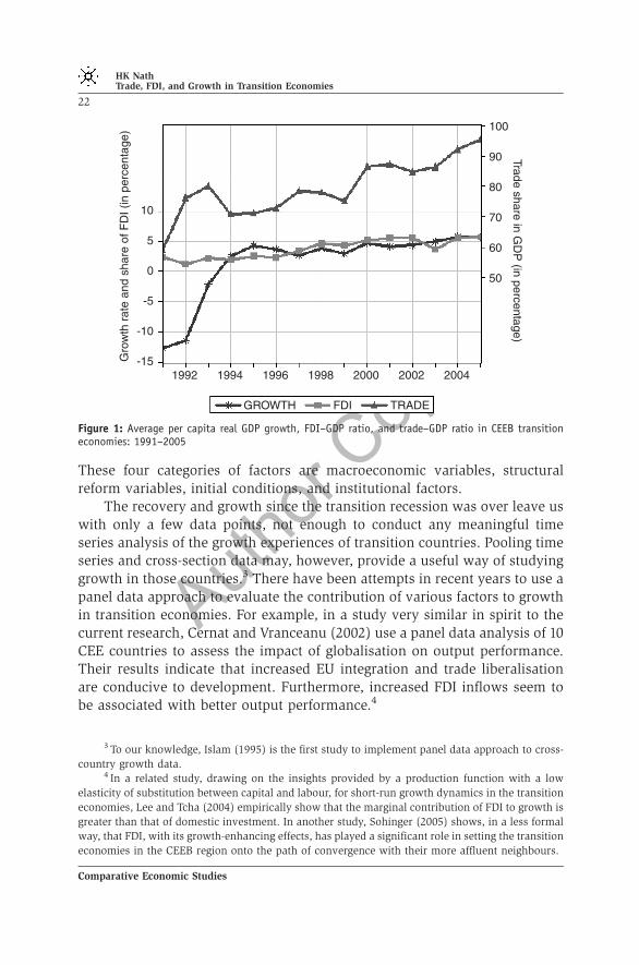
Figure 1 displays trends in growth of per capita real GDP, FDI-to-GDPratio, and volume of trade (exports plus imports) as a share of real GDP, alsoused as a measure of trade openness, all averaged across the cross-section of13 transition economies and expressed in percentages between 1991 and2005. As we can see, the average growth rate was negative until 1993. Then itfluctuated and has been steadily rising since 2001. The growth rates haveaveraged over 5% in the last 3 years of this period. The volume of tradeappears to have a clear upward trend. The FDI share has been increasingsteadily with some slow down in 2003.

The transition economies of CEEB experienced a substantial decline inoutput in the initial phase of transition, a phenomenon often referred to as thetransition recession. Fischer et al. (1996a) argue that restrictive macro-economic policies and restructuring of the economy caused such decline ineconomic activities. However, the extent and the speed of recovery variedacross countries. There is a substantial amount of literature that addressesvarious aspects of the transition recession and attempts to identify the factorsthat triggered the recovery. Some notable works include de Melo et al. (1996),Fischer et al. (1996a, b), Sachs (1996), de Melo et al. (1997), Hernandez-Cata(1997), Havrylyshyn et al. (1998), Berg et al. (1999), Polanec (2004), andPopov (2007). These studies examine one or more of four different sets ofvariables to understand the growth experiences of the early transition years.

1 These countries are Albania, Bulgaria, Croatia, Czech Republic, Estonia, Hungary, Latvia,

Lithuania, Macedonia FYR, Poland, Romania, Slovak Republic, and Slovenia. Ideally one would like

to include all transition economies in this investigation. But for some of the countries in the former

Soviet Union, reliable data are not available for a significant part of the sample period considered in

this paper.2 The numbers discussed and reported in this paragraph and the next are based on the author’s

calculation.

HK NathTrade, FDI, and Growth in Transition Economies

21

Comparative Economic Studies

Author

Copy

These four categories of factors are macroeconomic variables, structuralreform variables, initial conditions, and institutional factors.

The recovery and growth since the transition recession was over leave uswith only a few data points, not enough to conduct any meaningful timeseries analysis of the growth experiences of transition countries. Pooling timeseries and cross-section data may, however, provide a useful way of studyinggrowth in those countries.3 There have been attempts in recent years to use apanel data approach to evaluate the contribution of various factors to growthin transition economies. For example, in a study very similar in spirit to thecurrent research, Cernat and Vranceanu (2002) use a panel data analysis of 10CEE countries to assess the impact of globalisation on output performance.Their results indicate that increased EU integration and trade liberalisationare conducive to development. Furthermore, increased FDI inflows seem tobe associated with better output performance.4

10

-10

-15

5

-5

0

1992 1994 1996 1998 2000 2002 2004

GROWTH FDI TRADE

100

90

80

70

60

50

Trade share in GD

P (in percentage)

Gro

wth

rat

e an

d sh

are

of F

DI (

in p

erce

ntag

e)

Figure 1: Average per capita real GDP growth, FDI–GDP ratio, and trade–GDP ratio in CEEB transitioneconomies: 1991–2005

3 To our knowledge, Islam (1995) is the first study to implement panel data approach to cross-

country growth data.4 In a related study, drawing on the insights provided by a production function with a low

elasticity of substitution between capital and labour, for short-run growth dynamics in the transition

economies, Lee and Tcha (2004) empirically show that the marginal contribution of FDI to growth is

greater than that of domestic investment. In another study, Sohinger (2005) shows, in a less formal

way, that FDI, with its growth-enhancing effects, has played a significant role in setting the transition

economies in the CEEB region onto the path of convergence with their more affluent neighbours.


22


Author

Copy

In this paper we examine empirically the role of FDI and trade in theprocess of economic growth in 13 transition economies of the CEEB region.The empirical work is motivated primarily by an extension of the growththeory that includes trade and FDI as additional determinants of growth.Using fixed effects panel data estimation methods applied to data from1991 to 2005, this paper examines the effects of trade and FDI on growthafter controlling for gross domestic investment (GDI) and other macro-economic variables such as inflation, fiscal balance, size of the government,real money growth, the lending rate, and foreign exchange reserves;and structural variables such as tariff revenue and infrastructure reformindex.

This paper improves upon some previous work on growth in transitioneconomies by explicitly addressing three methodological issues. First, inorder to deal with the problem of omitted variables, a very generalspecification of the model including the largest possible number of variablesis estimated and F-tests are conducted to implement a ‘general-to-specific’approach of selecting the most parsimonious specification. Second, weconduct panel unit root tests to determine the stochastic trend properties ofthe variables. Nonstationary variables are included in the regression equationin their stationary forms. Furthermore, we formally test for groupwiseheteroscedasticity and cross-sectional correlation. The test results help uschoose the appropriate estimation technique. Third, by including the laggeddependent variable (LDV), we estimate a dynamic version of the model tomitigate the problem of serial correlation.

Our analysis suggests that a significant positive effect of trade on growthis a robust result for transition economies of the CEEB region. Additionally,domestic investment is an important determinant of growth. In general, FDIdoes not appear to have any significant effect on growth. When we control forthe effects of domestic investment and trade on FDI, however, it is found tohave a significant positive effect on growth, but only after 1995. Among otherfindings, macroeconomic stabilisation through fiscal and monetary policies asreflected in fiscal balance, size of the government, and real money growthplays a significant role. That the real lending rate turns out to be an importantdeterminant of growth underlines the importance of the development of thefinancial sector in transition economies. These results have important policyimplications.

The rest of the paper is organised as follows. The next section discussestheoretical background of the linkages between trade, FDI, and growth. In thesubsequent section, we describe the data and the methodology. Thesubsequent section presents the empirical results and analysis. In the lastsection, we summarise and include a few concluding remarks.


23


Author

Copy

LINKAGES BETWEEN TRADE, FDI, AND GROWTH: A THEORETICALBACKGROUND

The importance of trade and FDI for the growth of developing countries hasbeen emphasised in both theoretical and empirical literature. Apart from thetraditional Ricardian argument of efficiency gain from specialisation, therehave been several other hypotheses put forward to argue how trade mayaffect growth in developing countries. In early works (eg Rosenstein-Rodan,1943, Nurkse, 1953, Scitovsky, 1954, Fleming, 1955, Hirschman, 1958),exports were seen as providing the big push to break away from the viciouscycle of low-level equilibrium in which developing countries are often caught.Later, exports were thought to fill in the foreign exchange gap that preventedimports of machinery needed to be competitive in the market (see McKinnon,1964). More recently, Coe and Helpman (1995) argue that trade enhances thespillover effects of foreign R&D on domestic productivity. Another strand ofthe recent literature uses new growth theory framework to link trade policy togrowth. Externalities associated with liberal trade policies are seen as leadingto higher levels of GDP or higher growth.5

The importance of FDI for growth is emphasised for its role inaugmenting domestic capital stock and as a conduit for technology transfer,two essential elements in the modern growth literature.6 Studies that use thenew growth theory paradigm to examine the effects of FDI on growth taketwo different routes. For example, extending a hypothesis advanced byJagdish Bhagwati (1973), Balasubramanyam et al. (1996) were able to showthat the growth-enhancing effects of FDI were stronger in countries with amore liberal trade regime. They argue that a liberal trade regime is likely toprovide an appropriate environment conducive to learning that must go alongwith the human capital and new technology infused by FDI. Others (egBorensztein et al., 1998) rely on the absorptive capability of the recipientcountry in the form of stock of human capital for technological progress thatis assumed to take place through a process of capital deepening in the form ofnew varieties of capital goods introduced by FDI.

There are two dimensions to the hypothesis that FDI interacts with tradeto have a positive effect on growth. First, a more liberal trade environmentwith export orientation attracts larger FDI inflows because it not only allowsforeign capital to take advantage of low cost of labour in the host country butalso provides access to a larger market. Second, the neutrality of incentives

5 See Grossman and Helpman (1992) for a comprehensive discussion of a class of such models.6 In the literature, the role of FDI in transferring technology has received much attention and

spurred intense debate. For a recent survey, see Saggi (2002).


24


Author

Copy

associated with export orientation allows exploitation of economies of scale,better capacity utilisation, and a lower capital-output ratio, thus makingforeign capital more productive. Moreover, exports also promote technicalinnovation and dynamic learning from abroad and thereby create a morefavourable environment for externalities and learning from technologyspillovers associated with FDI.

Some of the recent theoretical work (Helpman et al., 2004; Antras andHelpman, 2004) has explored the relationship between trade and FDI. Undercertain conditions, trade and FDI have been shown to be substitutes. As thisline of research highlights the role of within-sector productivity differencesfor determining the patterns of international trade and FDI, it seems to haveimplications for growth in countries receiving the benefits of trade and/orFDI. For the purpose of our empirical study, the theoretical expositions of thelinkages between trade, FDI, and growth translate into an extended growthequation with trade and FDI as additional variables alongside domesticinvestment.

DATA AND METHODOLOGY

Data

The main sources of data for this study are the United Nations’ StatisticalDatabase, the Foreign Direct Investment Database compiled by the UnitedNations Conference on Trade and Development (UNCTAD), and theTransition Reports for various years prepared by the European Bank forReconstruction and Development (EBRD).

We obtain national accounts data on GDP per capita, gross fixedinvestment, government consumption expenditures, exports and imports ofgoods and services from the UN Statistical Database. These data are availableboth in national currency and in USD; and both at current prices and at 1990constant prices. We use constant 1990 USD data. We obtain the net FDIinflows data in current USD for CEEB countries from the UNCTAD.7 Oursample covers a period from 1990 to 2005.8

7 FDI inflows in the recipient economy ‘comprise capital provided (either directly or through

other related enterprises) by a foreign direct investor to an enterprise resident in the economy. FDI

flows are recorded on a net basis (capital account credits less debits between direct investors and

their foreign affiliates) in a particular year’ (UNCTAD).8 Although transition began in 1989 in most countries, data are either not available or too noisy

for this initial year of the process. When we calculate growth rates of per capita real GDP, we lose

one year’s data. Therefore, we use the sample period 1991–2005 in our estimation.


25


Author

Copy

It may be noted that the national accounts data on the transitioneconomies have serious problems, which have been emphasised by Fischeret al. (1996a) and others. The GDP data for years immediately after transitionare likely to overstate the decline of output and the increases in pricesbecause the pre-transition prices were used to measure output, which was ofextremely poor quality. Moreover, statistical agencies had been collecting andpublishing data on output mainly from the state sector and, therefore, theymay have underreported the expansion of the private sector during the initialyears of transition.

We construct the following variables for the empirical analysis. Thegrowth rate of per capita real GDP is calculated as 100 times first logdifferences of per capita real GDP and is used as the dependent variable(GROWTH) in the growth equation.9 Percentage share of exports plus importsin GDP is taken as a measure of the trade variable (TRADE). FDI inflow as apercentage share of GDP (in constant 1990 USD) is taken as the FDI variable(FDI). Note that FDI current price series has been converted into constant1990 USD by using an implicit deflator calculated from the series on gross

9 There have been studies that use per capita real GDP, mostly in logarithms, as the dependent

variable. For example, see Berg et al. (1999) and Cernat and Vranceanu (2002). Polanec (2004)

argues in favour of using growth rate of average labour productivity. There are others (eg Fischer

et al., 1996a, b; Sachs, 1996; de Melo et al., 1997) who use the growth rate of aggregate real GDP as

the dependent variable. There are some concerns, however, about the use of the growth rate of per

capita real GDP measured in 1990 constant USD. For example, the differences in the movements of

exchange rates over time across countries may introduce some systematic bias in the estimation of

the coefficients in our regression model when we use the growth rate of per capita real GDP

measured in constant USD instead of constant national currency as the dependent variable.

Furthermore, because of the differences in domestic prices across countries, there may have been

important differences even with growth rate of per capita real GDP measured in international

purchasing power parity (PPP) dollar. Ideally, one would like to use per capita real GDP in PPP

dollar, but data for all relevant variables measured in PPP dollars and for the sample period

considered are not readily available. To have a sense of the extent of possible biases, we examine

growth of per capita real GDP in 1990 constant national currency and growth of per capita real GDP

in international PPP dollar. We observe that growth rates of per capita real GDP in both US dollars

and in national currency track each other very closely, and for most countries they are perfectly

correlated. The correlation coefficient is the lowest with a value of 0.98 for Bulgaria. Thus, the bias

introduced by differences in movements of exchange rate should be negligible. We further obtain

growth rates of per capita real GDP measured in PPP dollar from Heston et al. (2006) for 1991–2004

(for some countries data are not available for all the years), plot them alongside growth rates of per

capita real GDP in 1990 USD, and calculate the correlation coefficients. The correlation ranges

between 0.825 (for Bulgaria) and 0.992 (for Croatia). For Albania, Bulgaria, Hungary, and Lithuania

the correlation coefficients are less than 0.90. Most of the deviations in these two sets of growth rates

are in the early years of transition. Interested readers can obtain the data and graphs from the author.

As mentioned above, these deviations are likely to introduce some biases in coefficient estimates.

However, the results do not seem to change qualitatively. The growth rates of per capita real GDP are

almost perfectly correlated with the growth rates of aggregate real GDP for all countries.


26


Author

Copy

fixed investment. FDI inflows are subtracted from gross fixed investment tocalculate GDI. The percentage share of GDI in GDP is taken as the domesticinvestment variable (GDI).

Additionally, data on CPI inflation, fiscal balance, nominal exchange rate,employment growth, money growth, domestic credit growth, lending rate,gross foreign exchange reserves, share of private sector in GDP, share ofindustry in employment, tariff revenues, budgetary subsidies and currenttransfers, and infrastructure reform index, the variables that are deemedimportant for growth, are obtained from various issues of EBRD’s TransitionReports.10 The Appendix includes a description of the variables along withavailability and sources of the data.

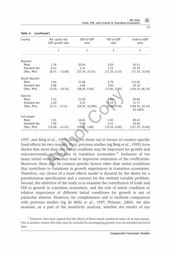
The summary statistics of the variables of interest (GROWTH, GDI, FDI,and TRADE) are presented in Table 1. Per capita real GDP in the CEEBcountries grew at an average rate of 1.63% during 1991–2005. The averagegrowth rate, however, varies widely across countries and so does its varianceover time. Among the CEEB countries, Poland has recorded the highestaverage annual rate of per capita real GDP growth, 3.43%, during this period,followed by Estonia, 3.08%. In Former Yugoslav Republic (FYR) ofMacedonia, the average annual growth rate has been negative. On anaverage, these countries have invested 18% of their GDP in building domesticstock of fixed capital during this period. Seven countries, Albania, CzechRepublic, Lithuania, Poland, Romania, Slovak Republic, and Slovenia, haveexceeded this average. FDI inflows have accounted for about 4% of real GDP,on average. This share is about 6% in the Czech Republic and above 8% inHungary. Average trade volume among these countries has been about 80%of GDP, with Estonia and Slovak Republic over 100%. In most countries, theincrease in this ratio over the sample period has been substantial.

Methodology

We use panel data estimation techniques for our empirical analysis. Asdiscussed above, extension of basic growth theory suggests that alongsidedomestic investment, trade, and FDI are important determinants of growth.We therefore consider GDI, FDI, and TRADE to be the main right-hand sidevariables in our growth equation. Although time invariant initial conditionshave been shown to be important for subsequent growth in general (see, eg,Barro, 1991) and for transition economies in particular (see de Melo et al.,

10 Data on other variables that may affect growth are also reported in the Transition Reports.

They are not included in our set of potentially relevant variables for one of two reasons: (i)

incomplete data with data missing for a significant part of our sample period; (ii) they represent the

same aspects of the economy as the ones that are included.


27


Author

Copy

Table 1: Summary statistics of the variables of interest: 1991–2005

Country Per capita realGDP growth rate

GDI-to-GDPratio

FDI-to-GDPratio

Trade-to-GDPratio

1 2 3 4

AlbaniaMean 2.94 18.72 2.14 42.74Standard dev 11.62 7.26 0.87 15.78(Max, Min) (12.69, �32.23) (29.21, 4.37) (3.77, 0.69) (95.30, 34.70)

BulgariaMean 1.31 10.06 4.65 86.52Standard dev 5.51 2.71 4.19 10.57(Max, Min) (6.20, �8.86) (15.66, 4.94) (14.56, 0.31) (108.40, 68.80)

CroatiaMean 0.36 16.97 3.60 65.44Standard dev 8.96 3.30 2.32 8.11(Max, Min) (7.35, �24.37) (22.97, 12.83) (7.17, 0.13) (78.20, 39.20)

Czech RepublicMean 1.43 22.55 5.95 94.17Standard dev 4.39 3.46 3.74 18.39(Max, Min) (5.93, �12.37) (28.55, 17.08) (12.35, 1.51) (124.80, 63.10)

EstoniaMean 3.08 14.40 4.94 112.71Standard dev 8.75 2.67 3.47 9.92(Max, Min) (11.70, �22.16) (19.63, 7.73) (15.54, 1.21) (131.30, 93.10)

HungaryMean 2.11 17.18 8.17 90.18Standard dev 4.68 5.16 2.61 28.28(Max, Min) (5.33, �12.48) (25.21, 7.05) (14.38, 3.29) (128.80, 45.40)

LatviaMean 0.68 14.53 3.46 72.91Standard dev 13.69 6.28 1.81 8.10(Max, Min) (10.66, �41.61) (26.40, 7.09) (7.14, 0.49) (87.30, 58.00)

LithuaniaMean 0.71 18.30 2.82 96.45Standard dev 10.34 2.95 2.13 19.43(Max, Min) (10.21, �23.68) (22.52, 14.19) (7.77, 0.12) (157.70, 71.00)

Macedonia, FYRMean �0.04 14.00 2.13 80.16Standard dev 3.88 3.97 2.91 11.70(Max, Min) (4.08, �9.10) (19.23, 1.80) (11.64, 0.00) (103.80, 58.80)

PolandMean 3.43 22.29 3.76 47.15Standard dev 3.50 2.96 1.94 9.90(Max, Min) (6.90, �7.63) (27.10, 17.86) (7.39, 0.38) (67.10, 34.50)


28


Author

Copy

1997, and Berg et al., 1999), we leave them out in favour of country-specificfixed effects for two reasons. First, previous studies (eg Berg et al., 1999) haveshown that more than one initial condition may be important for growth andmacroeconomic performance in transition economies.11 Inclusion of toomany initial conditions may lead to imprecise estimation of the coefficients.Moreover, there may be country-specific factors other than initial conditionsthat contribute to variations in growth experiences in transition economies.Therefore, our choice of a fixed effects model is dictated by the desire for aparsimonious specification and a concern for the omitted variable problem.Second, the objective of the study is to examine the contribution of trade andFDI to growth in transition economies, and the role of initial condition orrelative importance of different initial conditions for growth is not ofparticular interest. However, for completeness and to facilitate comparisonwith previous studies (eg de Melo et al., 1997; Polanec, 2004), we alsoexamine, as a part of the sensitivity analysis, whether the results of our

Table 1: (continued )

Country Per capita realGDP growth rate

GDI-to-GDPratio

FDI-to-GDPratio

Trade-to-GDPratio

1 2 3 4

RomaniaMean 1.18 20.64 3.63 54.41Standard dev 6.51 2.34 3.14 10.79(Max, Min) (8.57, �13.68) (23.76, 15.24) (11.32, 0.15) (71.10, 33.40)

Slovak RepublicMean 1.94 21.68 3.76 112.56Standard dev 5.98 4.86 3.83 18.19(Max, Min) (5.93, �16.16) (28.20, 9.56) (14.84, 0.92) (140.10, 86.10)

SloveniaMean 2.12 23.20 1.86 90.83Standard dev 4.20 4.37 2.10 11.71(Max, Min) (5.11, �9.74) (29.32, 16.000) (9.03, 0.56) (108.70, 63.10)

63.1095)

Full sampleMean 1.63 18.04 3.93 80.43Standard dev 7.58 5.77 3.31 26.56(Max, Min) (12.69, �41.61) (29.32, 1.80) (15.54, 0.00) (157.70, 33.40)

11 However, they have argued that the effects of these initial conditions taper off as time passes.

This is another reason why they may be excluded in investigating growth over an extended period of

time.


29


Author

Copy

empirical analysis are robust enough to include the initial conditions in thegrowth equation.

Although growth theory provides some guidance, growth in countriesthat are going through economic and political transition could just be a blackbox. Therefore, choosing appropriate control variables is a difficult task. Asshown by previous works, growth in transition economies may well beaffected by, in addition to initial conditions, macro variables, structuralreform variables, and institutional factors. Based on suggestions fromprevious works and data availability, we choose two categories of variables:macroeconomic variables and structural reform variables. The first categoryincludes CPI inflation (INF), fiscal balance as percentage of GDP (FBAL), sizeof the government as measured by the percentage share of governmentconsumption expenditures in GDP (GOV), nominal exchange rate (X),employment growth (EMP), real money growth (MONEY), real domesticcredit growth (DOMCREDIT), real lending rate (LRATE), and gross foreignexchange reserves as a percentage share of GDP (RES).

These variables either reflect the effects of macroeconomic stabilisationpolicies or represent macroeconomic factors that potentially affect growth.For example, like Berg et al. (1999), we use inflation as a stabilisation proxy.Fiscal balance is expected to affect growth through crowding out andgovernment consumption expenditures through a short-run aggregatedemand stimulus. The nominal exchange rate captures the effect of exchangerate targeting in stabilisation policies. However, because these countriesadopted different exchange rate regimes and they made changes, somedrastic, over the time it is difficult to speculate on the effects of the exchangerate on growth.12 Employment growth is expected to affect growth throughaugmentation of the labour stock. Real money growth, domestic creditgrowth, and the lending rate are assumed to capture real effects of monetarypolicy and of developments in the financial sector. Gross foreign exchangereserves are expected to contribute to growth by alleviating the foreignexchange constraint for trade and investment.

The category of structural variables includes the share of private sector inGDP (PVT), tariff revenue as a percentage of total imports (TARIFF),budgetary subsidies and current transfers as a percentage share of GDP(SUB), percentage share of industry in total employment (INDEMP), andinfrastructure reform index (INFRA). The first variable is an indicator of thespeed and extent of structural reform and is expected to have a positive effecton growth through increased efficiency. TARIFF measures the extent of trade

12 For a discussion on exchange rate regime, stabilisation, and growth in transition economies,

see Fischer et al. (1996a).


30


Author

Copy

liberalisation. Budgetary subsidies to enterprises and households areexpected to have a positive effect on growth by encouraging investment,thus galvanising aggregate demand. The share of industry in total employ-ment reflects the relative size of the labour force engaged in electricity, power,manufacturing, mining, and water, and a larger share in those crucial sectorsis assumed to contribute positively to growth through structural change of theeconomy. The infrastructure reform index is expected to capture the effects ofimprovements in transportation, communication, and power generation ongrowth.13 Country-specific fixed effects will capture some of the importantdifferences in institutions across the transition economies.14

We estimate a pooled time-series cross-section regression of the followingform:

git ¼ mi þ b0Xit þ g0Zit þ eit

where git is the annual growth rate of per capita real GDP for country i in yeart; mi is the country-specific fixed effect; Xit is the vector of variables of interest:GDI, FDI, and TRADE; and Zit is the vector of control variables; i¼ 1, 2,y Nindexes country and t¼ 1, 2,y T indexes time.

Among various issues and concerns about this empirical methodology,the following have been formally addressed. First, nonstationarity of time-series data is often a cause for concern for meaningful analysis of the databecause it may lead to a spurious relationship. The conventional univariateunit root tests suffer from lack of power when the length of the sample periodis short. The panel unit root tests, which are relatively new techniques,supposedly alleviate the problem of lack of power by combining data in timeand cross-section dimensions. We, therefore, conduct panel unit root tests onthe variables of interest as well as on all potential control variables. We usetwo most commonly used test procedures suggested by Levin et al. (2002)and Im et al. (2003), respectively. The first test assumes a common unit rootprocess for all cross-sectional units whereas the second assumes different unitroot processes for individual cross-sectional units. Both methods have theiradvantages and disadvantages (see Baltagi (2002) for a discussion).

Second, given the differences in growth experiences among transitioneconomies, one would expect tremendous variation of variables in the model.Moreover, geographic contiguity, and similarity and links between erstwhile

13 Intuitively some of the variables are expected to affect one another and, therefore, to be

correlated. Our general-to-specific approach of model selection should eliminate the possible

collinearity among the variables.14 Grogan and Moers (2001) present a cross-section analysis of 25 transition economies to show

that institutions are important for growth and FDI.


31


Author

Copy

political systems make it likely that there are some common factors that affectthese countries. We, therefore, formally test for groupwise heteroscedasticityand cross-sectional correlation. Following Greene (1997), we conduct simpleLagrange multiplier (LM) Tests. For serial autocorrelation, however, we relyon pooled Durbin–Watson (DW) test statistics. These tests also help usdetermine the appropriate estimation method.

Third, although country fixed effects take care of time invariant country-specific factors, the model may still suffer from an omitted variable problem ifsome important time-variant control variables are not included. Moreover,some of these variables may be correlated with each other. Thus, whileexclusion of relevant variables may lead to the omitted variables problem,inclusion of them may give rise to the problem of collinearity. To addressthese problems, we first estimate a general model including all controlvariables listed above. The obvious drawback of including many variables isthat, given lack of degrees of freedom, the coefficients are impreciselyestimated. If some variables have negligible effects, excluding them wouldlead to more precise estimates. Moreover, multicollinearity may show up interms of statistically insignificant individual coefficient with high R2.Remedies of this problem include exclusion of variables that are collinearwith others. We therefore adopt a less stringent application of Hendry(1995)’s general-to-specific approach. We then apply a sequence of F-tests toreduce the model to more parsimonious specifications admissible under ourdata set. We start with excluding a single variable under each category ofcontrol variables, and then we test for exclusion of an entire category ofvariables. This general-to-specific approach would help us find the mostparsimonious specification of our model.15

EMPIRICAL RESULTS

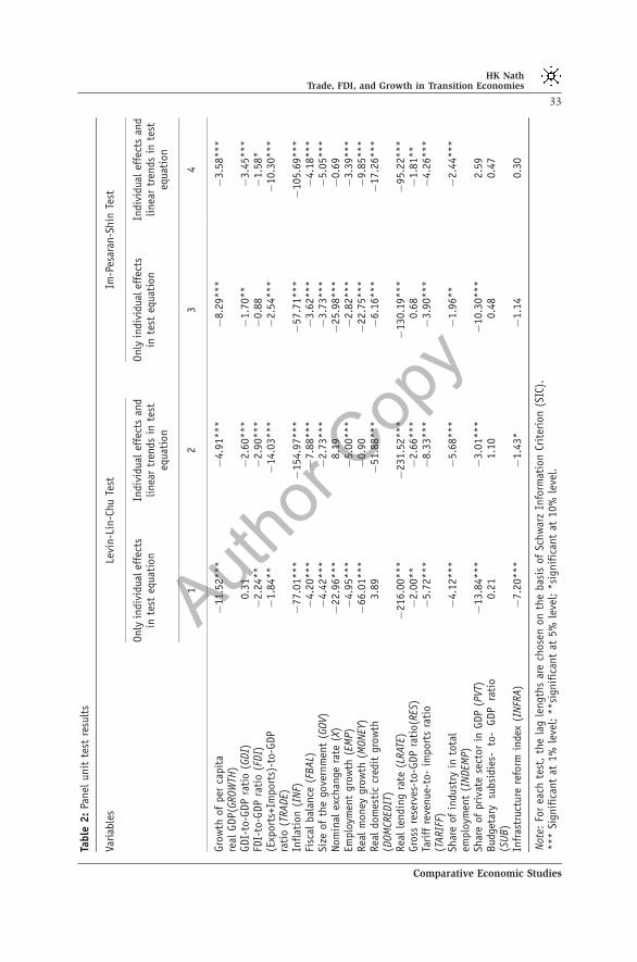
Table 2 presents the results of the panel unit root tests conducted on growth ofper capita real GDP and all other variables that are potential determinants ofgrowth. Specifying the test equation under both Levin-Lin-Chu and Im-Pesaran-Shin test procedures is a formidable task. Because there are no clear-cut guidelines, we conduct these tests under two specifications: with onlyindividual effects in the test equation, and with both individual effects andlinear time trends. As we can see from the table, for GDI, FDI, X, DOMCREDIT,

15 Note that we do not apply the general-to-specific approach to our variables of interest.

Therefore, even in the most parsimonious specification, a multicollinearity problem may arise if two

or more of these variables are collinear.


32


Author

Copy

Table

2:

Panel

unit

test

resu

lts

Variab

les

Levi

n-L

in-C

hu

Test

Im-P

esar

an-S

hin

Test

Only

indiv

idua

lef

fect

sin

test

equa

tion

Indiv

idua

lef

fect

san

dlinea

rtr

ends

inte

steq

uati

on

Only

indiv

idua

lef

fect

sin

test

equa

tion

Indiv

idua

lef

fect

san

dlinea

rtr

ends

inte

steq

uati

on

12

34

Gro

wth

ofper

capit

are

alGDP(G

ROW

TH)

�11.5

2***

�4.9

1**

*�

8.2

9**

*�

3.5

8**

*

GDI-

to-G

DP

rati

o(G

DI)

0.3

1�

2.6

0**

*�

1.7

0**

�3.4

5**

*FD

I-to

-GDP

rati

o(F

DI)

�2.2

4**

�2.9

0**

*�

0.8

8�

1.5

8*

(Exp

ort

s+Im

port

s)-t

o-G

DP

rati

o(T

RADE)

�1.8

4**

�14.0

3***

�2.5

4**

*�

10.3

0***

Inflat

ion

(INF)

�77.0

1***

�154.9

7***

�57.7

1***

�105.6

9***

Fisc

albal

ance

(FBAL)

�4.2

0**

*�

7.8

8**

*�

3.6

2**

*�

4.1

8**

*Si

zeof

the

gove

rnm

ent

(GOV)

�4.4

2**

*�

2.7

3**

*�

3.7

3**

*�

5.0

5**

*Nom

inal

exch

ange

rate

(X)

�22.9

6***

8.1

9�

25.9

8***

�0.6

9Em

plo

ymen

tgro

wth

(EM

P)

�4.9

5**

*�

5.0

0**

*�

2.8

2**

*�

3.3

9**

*Rea

lm

oney

gro

wth

(MONEY

)�

66.0

1***

�0.9

0�

22.7

5***

�9.8

5**

*Rea

ldo

mes

tic

cred

itgro

wth

(DOM

CRED

IT)

3.8

9�

51.8

8***

�6.1

6**

*�

17.2

6***

Rea

lle

ndin

gra

te(L

RAT

E)�

216.0

0***

�231.5

2***

�130.1

9***

�95.2

2***

Gro

ssre

serv

es-t

o-G

DP

rati

o(R

ES)

�2.0

0**

�2.6

6**

*0.6

8�

1.8

1**

Tari

ffre

venue-

to-

impor

tsra

tio

(TARIF

F)�

5.7

2**

*�

8.3

3**

*�

3.9

0**

*�

4.2

6**

*

Shar

eof

indu

stry

into

tal

emplo

ymen

t(I

NDEM

P)

�4.1

2**

*�

5.6

8**

*�

1.9

6**

�2.4

4**

*

Shar

eof

pri

vate

sect

or

inGDP

(PVT

)�

13.8

4***

�3.0

1**

*�

10.3

0***

2.5

9Bud

geta

rysu

bsi

die

s-to

-GDP

rati

o(S

UB)

0.2

11.1

00.4

80.4

7

Infr

astr

uctu

rere

form

inde

x(I

NFR

A)

�7.2

0**

*�

1.4

3*

�1.1

40.3

0

Not

e:Fo

rea

chte

st,

the

lag

length

sar

ech

ose

non

the

bas

isof

Schw

arz

Info

rmat

ion

Crit

erio

n(S

IC).

***

Signif

ican

tat

1%

leve

l;**si

gnif

ican

tat

5%

leve

l;*si

gnif

ican

tat

10%

leve

l.


33


Author

CopyRES, and INFRA, the results are mixed. While we can reject the null of unit

root under some specifications we cannot do so under others. Because in atleast two out of four specifications we do not find them to be unit rootprocesses, we assume that these variables are stationary. Only for SUB do theresults unequivocally indicate that it is a unit root process. Therefore, we usethe first difference, which is the stationary form, of SUB in our estimation ofthe regression equation.

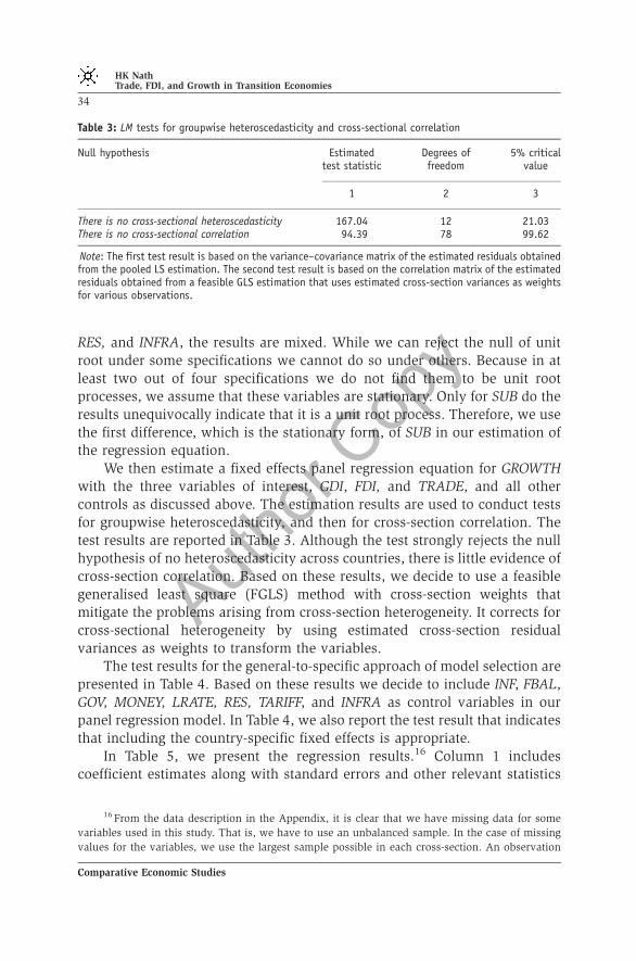
We then estimate a fixed effects panel regression equation for GROWTHwith the three variables of interest, GDI, FDI, and TRADE, and all othercontrols as discussed above. The estimation results are used to conduct testsfor groupwise heteroscedasticity, and then for cross-section correlation. Thetest results are reported in Table 3. Although the test strongly rejects the nullhypothesis of no heteroscedasticity across countries, there is little evidence ofcross-section correlation. Based on these results, we decide to use a feasiblegeneralised least square (FGLS) method with cross-section weights thatmitigate the problems arising from cross-section heterogeneity. It corrects forcross-sectional heterogeneity by using estimated cross-section residualvariances as weights to transform the variables.

The test results for the general-to-specific approach of model selection arepresented in Table 4. Based on these results we decide to include INF, FBAL,GOV, MONEY, LRATE, RES, TARIFF, and INFRA as control variables in ourpanel regression model. In Table 4, we also report the test result that indicatesthat including the country-specific fixed effects is appropriate.

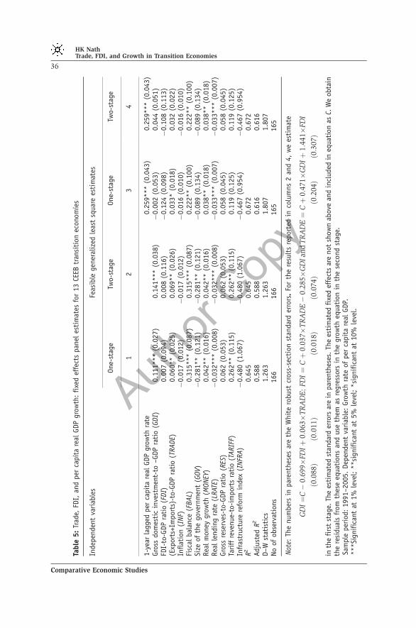
In Table 5, we present the regression results.16 Column 1 includescoefficient estimates along with standard errors and other relevant statistics

Table 3: LM tests for groupwise heteroscedasticity and cross-sectional correlation

Null hypothesis Estimatedtest statistic

Degrees offreedom

5% criticalvalue

1 2 3

There is no cross-sectional heteroscedasticity 167.04 12 21.03There is no cross-sectional correlation 94.39 78 99.62

Note: The first test result is based on the variance–covariance matrix of the estimated residuals obtainedfrom the pooled LS estimation. The second test result is based on the correlation matrix of the estimatedresiduals obtained from a feasible GLS estimation that uses estimated cross-section variances as weightsfor various observations.

16 From the data description in the Appendix, it is clear that we have missing data for some

variables used in this study. That is, we have to use an unbalanced sample. In the case of missing

values for the variables, we use the largest sample possible in each cross-section. An observation


34


Author

Copy

estimates from the FGLS method, which we will call the one-stage/single-stage method in order to distinguish it from its alternative. Note that thestandard errors are estimated using White’s heteroskedasticity consistentvariance–covariance estimates that are robust to general heteroskedasticity.Column 2 presents estimates obtained from the two-stage estimation process.Intuitively, GDI, FDI, and TRADE may affect each other.17 Therefore, weestimate an equation for each of these three variables, using another two asregressors in the first stage, obtain the residual and use it as a regressor in ourgrowth equation in the second stage. For example, we regress GDI on FDI andTRADE, FDI on GDI and TRADE, and TRADE on GDI and FDI and extract theresiduals, which are then included as explanatory variables in the growth

Table 4: F-test results for exclusion of control variables and fixed effects

Category ofvariables

Variable F-statistics Degreesof freedom

P-value

1 2 3 4

Macroeconomicvariables

Inflation (INF) 4.15** (1,118) 0.04Fiscal balance (FBAL) 7.18** (1,118) 0.01Size of the government (GOV) 16.45*** (1,118) 0.00Exchange rate (X) 0.31 (1,118) 0.58Employment growth (EMP) 1.40 (1,118) 0.24Real money growth (MONEY) 2.76* (1,118) 0.09Real domestic credit growth (DOMCREDIT) 2.32 (1,118) 0.13Real lending rate (LRATE) 63.66*** (1,118) 0.00Gross reserves-to-GDP ratio (RES) 7.06** (1,118) 0.01All macro variables 14.20*** (9,118) 0.00

Structuralvariables

Tariff revenue-to-imports ratio (TARIFF) 10.40*** (1,118) 0.00Share of industry in total employment (INDEMP) 0.04 (1,118) 0.84Share of private sector in GDP (PVT) 0.14 (1,118) 0.71Budgetary subsidies- to- GDP ratio (SUB) 1.55 (1,118) 0.21Infrastructure reform index (INFRA) 14.59*** (1,118) 0.00All structural variables 4.26*** (5,118) 0.00

Fixed effects 5.96*** (12,118) 0.00

***Significant at 1% level; **significant at 5% level; *significant at 10% level.

will be excluded from the estimation of our regression model if any of the explanatory or dependent

variables for that cross-section are unavailable in that period.17 There is some evidence of mutual relationship among GDI, FDI, and TRADE. For example,

Campos and Kinoshita (2003) find that trade has a positive effect on FDI in transition economies.

Kutan and Vuksic (2007) further investigate the effects of FDI on the export performance of 12 CEE

countries and find that while FDI has increased exports by increasing supply capacity through

augmentation of the physical capital stock in all countries in their sample, it has helped exports

through FDI-specific effects such as technology transfer, higher productivity, and information about

export markets, only among the new members of the European Union.


35


Author

Copy

Table

5:

Trad

e,FD

I,an

dper

capit

are

alGDP

gro

wth

:fi

xed

effe

cts

pan

eles

tim

ates

for

13

CEEB

tran

siti

on

econom

ies

Inde

pen

dent

variab

les

Feas

ible

gener

aliz

edle

ast

squa

rees

tim

ates

One-

stag

eTw

o-s

tage

One-

stag

eTw

o-s

tage

12

34

1-y

ear

lagge

dper

capit

are

alGDP

gro

wth

rate

0.2

59***

(0.0

43)

0.2

59***

(0.0

43)

Gro

ssdo

mes

tic

inve

stm

ent-

to–GDP

rati

o(G

DI)

0.1

11*

**

(0.0

27)

0.1

41***

(0.0

38)

�0.0

02

(0.0

53)

0.0

44

(0.0

51)

FDI-

to-G

DP

rati

o(F

DI)

0.0

07

(0.0

94)

0.0

08

(0.1

16)

�0.1

24

(0.0

98)

�0.1

08

(0.1

13)

(Exp

ort

s+Im

port

s)-t

o-G

DP

rati

o(T

RADE)

0.0

60*

*(0

.025)

0.0

69**

(0.0

26)

0.0

33*

(0.0

18)

0.0

32

(0.0

22)

Inflat

ion

(INF)

�0.0

17

(0.0

12)

�0.0

17

(0.0

12)

�0.0

16

(0.0

10)

�0.0

16

(0.0

10)

Fisc

albal

ance

(FBAL)

0.3

15*

**

(0.0

87)

0.3

15***

(0.0

87)

0.2

22**

(0.1

00)

0.2

22**

(0.1

00)

Size

ofth

ego

vern

men

t(G

OV)

�0.2

81*

*(0

.121)

�0.2

81**

(0.1

21)

�0.0

89

(0.1

34)

�0.0

89

(0.1

34)

Rea

lm

oney

gro

wth

(MONEY

)0.0

42*

*(0

.016)

0.0

42**

(0.0

16)

0.0

38**

(0.0

18)

0.0

38**

(0.0

18)

Rea

lle

ndin

gra

te(L

RAT

E)�

0.0

32*

**

(0.0

08)

�0.0

32***

(0.0

08)

�0.0

33***

(0.0

07)

�0.0

33***

(0.0

07)

Gro

ssre

serv

es-t

o-G

DP

rati

o(R

ES)

0.0

62

(0.0

53)

0.0

62

(0.0

53)

0.0

58

(0.0

45)

0.0

58

(0.0

45)

Tari

ffre

venue-

to-i

mpor

tsra

tio

(TARIF

F)0.2

62*

*(0

.115)

0.2

62**

(0.1

15)

0.1

19

(0.1

25)

0.1

19

(0.1

25)

Infr

astr

uctu

rere

form

inde

x(I

NFR

A)

�0.4

80

(1.0

67)

�0.4

80

(1.0

67)

�0.4

67

(0.9

54)

�0.4

67

(0.9

54)

R2

0.6

45

0.6

45

0.6

72

0.6

72

Adju

sted

R2

0.5

88

0.5

88

0.6

16

0.6

16

D–W

stat

isti

cs1.2

63

1.2

63

1.8

07

1.8

07

No

ofobse

rvat

ions

166

166

165

165

Not

e:Th

enum

ber

sin

par

enth

eses

are

the

Whit

ero

bust

cross

-sec

tion

stan

dard

erro

rs.

For

the

resu

lts

report

edin

colu

mns

2an

d4,

we

esti

mat

e

GD

I¼

C�

0:6

99�

FDIþ

0:0

63�

TR

AD

E;

FDI¼

Cþ

0:0

37�

TR

AD

E�

0:2

85�

GD

Ian

dT

RA

DE¼

Cþ

0:4

71�

GD

Iþ

1:4

41�

FDI

ð0:0

88Þ

ð0:0

11Þ

ð0:0

18Þ

ð0:0

74Þ

ð0:2

04Þ

ð0:3

07Þ

inth

efi

rst

stag

e.Th

ees

tim

ated

stan

dard

erro

rsar

ein

par

enth

eses

.Th

ees

tim

ated

fixe

def

fect

sar

enot

show

nab

ove

and

incl

uded

ineq

uati

on

asC.

We

obta

inth

ere

sidu

als

from

thes

eeq

uati

ons

and

use

them

asre

gre

ssor

sin

the

gro

wth

equa

tion

inth

ese

cond

stag

e.Sa

mple

per

iod:

1991–200

5.

Dep

ende

nt

variab

le:

Gro

wth

rate

ofper

capit

are

alGDP.

***Si

gnif

ican

tat

1%

leve

l;**si

gnif

ican

tat

5%

leve

l;*si

gnif

ican

tat

10%

leve

l.


36


Author

Copy

equation. Thus, GDI now represents the residual variation in domesticinvestment after controlling for the effects of FDI and TRADE. Similarly, FDIand TRADE reflect residual variations in FDI and trade, respectively, aftercontrolling for the effects of the remaining two variables of interest.

The results indicate that among the variables of interest, trade has asignificant positive effect on per capita real GDP growth, and this result isrobust under alternative estimation methods. The single-stage FGLS estimateindicates that a 1% point increase in TRADE increases per capita real GDPgrowth rate by about 0.06% point, whereas two-stage estimate indicates aslightly larger effect, 0.068. Domestic investment also has significant positiveeffect on the per capita growth rate. A 1% point increase in GDI leads to abouta 0.11% point increase in per capita GDP growth rate in single-stage estimate,whereas the effect is larger, 0.141, when the two-stage estimation method isused. Although the effect of FDI on per capita growth is positive, it isstatistically not significant. It may be noted that GDI and FDI have asignificant negative relationship, as revealed by the first-stage estimates,which may be suggestive of crowding out as a result of FDI in transitioneconomies. GDI and TRADE, and TRADE and FDI are found to havesignificant positive relationships indicating complementary roles betweenthem.

Among the control variables, significant positive effects of fiscal balanceand real money growth and significant negative effects of size of thegovernment and real lending rate are robust across specifications. Thesignificant effect of fiscal balance accords well with the previous study byBerg et al. (1999), and highlights the importance of macroeconomicstabilisation for growth of the transition economies of the CEEB region.Contrary to our expectation of a positive effect of GOV through its effect onaggregate demand, the size of the government has significant negative effecton growth. This may reflect inefficiency associated with large government.Although inflation appears to have a negative effect, it is not statisticallysignificant. The significant positive effect of real money growth may havehighlighted the aggregate demand stimulus of money supply growth.Furthermore, that real lending rate has significant negative effect suggeststhat tighter credit market conditions adversely affect growth. The significantpositive impact of tariff is, however, counterintuitive. One might suspect thatthere is collinearity between TRADE and TARIFF, but exclusion of TRADEdoes not render the coefficient negative nor makes it statistically insignificant.The result may just reflect better enforcement of tariff laws.

We report the pooled DW test statistics for all three methods and theyindicate that the null of no serial correlation is rejected at a 5% significancelevel. We therefore estimate a dynamic version of the equation including the


37


Author

Copy

LDV. As LDV is correlated with country-specific fixed factors, it rendersestimates of the coefficients biased and inconsistent. Note that only if T-N,the least squares estimates will be consistent for the dynamic error panelmodel. Some researchers, for example Islam (1995), favour least squaresestimates for moderate size T if N is relatively large, arguing that the bias maynot be large in those cases.18 The trade coefficient is statistically significant ata 10% level when single-stage FGLS is used. The two-stage estimate is,although positive, not statistically significant. Both GDI and FDI have negativesigns under single-stage FGLS, and neither is statistically significant. Undertwo-stage estimation, the coefficient estimate of GDI becomes positive butremains statistically insignificant. Even long-run effects of these variables,calculated by multiplying the estimated coefficients by 1/(1�r̂) where r̂ is theestimated coefficient of the LDV, are smaller than those in the static model.Note that the earlier results about the effects of the control variables arerobust to this dynamic specification of the model except that GOV and TARIFFare no longer significant. The DW statistics in the LDV models suggest thatthe issue of autocorrelation is resolved.

Sensitivity analysis

We conduct three different sensitivity exercises. First, because the relativeimportance of initial conditions and reform measures is one of the centraltopics in the growth literature on the transition economies, we will examinewhether our results with regard to the effects of trade, FDI, and GDI ongrowth hold when we explicitly introduce initial conditions and reformmeasures in our regression models. We experiment with three different sets ofinitial conditions.

We first use the logarithm of per capita real GDP in 1990 for the CEEBcountries as the initial conditions. Some studies (de Melo et al., 1996; Fischeret al., 1996a, b) use this variable as the only initial condition. The neoclassicalgrowth model predicts that countries with higher initial per capita incomewill experience slower growth compared to countries with lower initial percapita income. However, as de Melo et al. (1997) argue, in addition to initialper capita income, there may be a host of initial conditions representing initiallevel of development, resources and growth, initial economic distortions, andinstitutional characteristics that are important for growth in the transition

18 See Baltagi (2002 pp. 129–30) for a discussion. Many alternatives for getting around the

problems associated with dynamic specification of fixed effects model have been suggested. Notable

works include Anderson and Hsiao (1981), Arellano (1989), and Arellano and Bond (1991).


38


Author

Copy

economies. Following their suggestions, we consider 11 initial conditions: percapita real GDP in 1990 (Y1990); the average annual growth rate between1985 and 1989 (PRGR); urbanisation in 1990 (URBAN); a dummy variable forrichness in terms of natural resources (RICH); a categorical variable forwhether the country was an independent state, part of a federal state, or anewly created country (STATE); black market exchange rate premium(BLCMKT); extent of overindustrialisation in 1990 (INDIST); a dummyvariable for whether the country is neighbouring a thriving market economy(LOCAT); repressed inflation (REPR); trade dependence (TDEP); and the timeunder central planning (MARME).19 For details on these conditions, see deMelo et al. (1997). Finally, we also consider a set of eight initial conditions assuggested by Polanec (2004). In addition to the last six initial conditions of deMelo et al. (1997), this set also includes price liberalisation index (PLI) andtrade liberalisation index (TLI) in 1990 published by EBRD.

As for reform measures, following Polanec (2004) we use the year-to-yearchange in an unweighted average of EBRD transition indicators (DREFORM).There are eight indicators that cover large- and small-scale privatisation,enterprise restructuring, price liberalisation, trade and forex system,competition policy, banking reform and interest rate liberalisation, securitiesmarkets and nonbank financial institutions, and overall infrastructure reform.The values of these indicators range from 1 to 4 and are based on subjectivejudgments of country economists at the EBRD. Furthermore, as Polanec(2004) points out, by using these indicators we are assuming that the effectsof reforms on growth are the same at various stages of reform, which may behighly unlikely.

As discussed by de Melo et al. (1997) and Polanec (2004), these initialconditions may be highly correlated and, therefore, inclusion of all thesetime-invariant conditions may introduce the problem of multicollinearity. Inorder to reduce the dimensionality of the set of initial conditions and to findan appropriate common interpretation, we resort to the method of principalcomponents. For the set of 11 initial conditions, the first two componentsaccount for about 60% of variability in initial conditions. The most importantcluster has high positive factor loadings for TDEP, BLCMKT, MARME, URBAN,and REPR, and has high negative factor loading for STATE. Except for URBAN,this cluster looks very similar to PRIN1 in de Melo et al. (1997), which theyinterpret as a measure of macroeconomic distortions. The second mostimportant cluster has high positive factor loading for REPR, RICH, INDIST,BLCMKT, and high negative factor loading for LOCAT and Y1990. In this case,

19 Except for initial per capita real GDP, for other initial condition variables we use the same

acronyms as de Melo et al. (1997).


39


Author

Copy

the similarity with PRIN2 in de Melo et al. (1997) ends in high positive factorloadings for INDIST. Given that we consider only a subset of the countries intheir sample, this is not surprising. We include these two clusters (IC_cluster1and IC_cluster2) in one of the specifications of the panel regression modelwith initial conditions.

For the next set of eight initial conditions that we consider, the firstprincipal component explains about 45% of variability. The most importantcluster of these conditions, has high positive factor loadings for BLCMKT,TDEP, MARME, and REPR, and has negative factor loadings for both PLI andTLI. Although the factor loadings are smaller in value than those obtained byPolanec (2004), they are qualitatively very similar. We include this cluster(IC_cluster) along with the initial per capita real GDP in an alternativespecification of our panel regression model. Note that a table (Table A1)presenting the factor loadings for all the principal components discussedabove is included in the Appendix.

The results from two-stage estimation of these alternative specificationswith initial conditions and reform measures are presented in Table 6.Columns 1–3 present the results when only the initial conditions areincluded in panel regression model. As we can see, significant negativeeffect of per capita real GDP in 1990 is a robust result. IC_cluster1 andIC_cluster2 do not have any significant impact on growth. When the cluster ofeight initial conditions is included along with 1990 per capita realGDP, however, it appears to have significant positive effect on growth.20

The fact that there are some similarities between IC_cluster1 and IC_clusterin terms of factor loadings seems to suggest that this positive significanteffect may have been driven by price and trade liberalisation in 1990. In allcases, GDI has a significant positive effect on growth. The estimatedcoefficient of FDI is not statistically significant under any of the specifications.TRADE has a statistically significant positive effect on growth under allspecifications.

20 An experiment with the sample period 1991–1995 reveals that IC_cluster1 has significant

negative, IC_cluster2 has significant positive, and IC_cluster has significant negative effects on

growth. Although the result for IC_cluster1 accords well with de Melo et al. (1997), the result for

IC_cluster2 does not seem to conform to these results. This may be due to some important

interactions the IC-cluster2 may have with the control variables included in our regression model.

The result for the IC_cluster, on the other hand, accords well with the result of Polanec (2004) for the

period 1990–1994. The estimated coefficient of Y1990 is negative and statistically significant under

all specifications and estimation methods. We do not report the results to save space. Interested

readers can obtain the results of this experiment, and also the one-stage estimation results for

specifications in Table 6 from the author.


40


Author

Copy

Table

6:

Trad

e,FD

I,an

dper

capit

are

alGDP

gro

wth

:fi

xed

effe

cts

pan

eles

tim

ates

for

13

CEEB

tran

siti

on

econom

ies

Indep

ende

nt

vari

able

s1

23

45

67

1990

Per

capit

are

alGDP

(Y1990)�

1.0

87***

(0.3

39)

�0.6

99*

(0.3

85)

�1.0

52***

(0.3

46)

�0.7

37*

(0.3

94)

Clust

erof

8in

itia

lco

ndit

ions

(IC_

clust

er)

0.2

48***

(0.0

69)

0.2

45***

(0.0

64)

Clust

erof

11

init

ial

condit

ions

1(I

C_cl

ust

er1)

0.3

79

(0.2

91)

0.4

92*

(0.2

52)

Clust

erof

11

init

ial

condit

ions

2(I

C_cl

ust

er2)

�0.0

55

(0.3

63)

�0.2

55

(0.3

06)

Gro

ssdo

mes

tic

inve

stm

ent-

to-G

DP

rati

o(G

DI)

0.1

15***

(0.0

39)

0.1

95***

(0.0

47)

0.1

79***

(0.0

44)

0.0

88**

(0.0

37)

0.0

57

(0.0

45)

0.1

16**

(0.0

48)

0.1

09**

(0.0

43)

FDI-

to-G

DP

rati

o(F

DI)

�0.0

20

(0.1

18)

0.0

07

(0.1

40)

�0.0

15

(0.1

30)

�0.0

15

(0.0

95)

�0.0

45

(0.1

00)

�0.0

24(0

.116)

�0.0

57

(0.1

07)

(Exp

ort

s+Im

port

s)-t

o-G

DP

rati

o(T

RADE)

0.0

38*

(0.0

21)

0.0

73***

(0.0

25)

0.0

62***

(0.0

22)

0.0

53***

(0.0

17)

0.0

24

(0.0

16)

0.0

57***

(0.0

21)

0.0

44**

(0.0

18)

Inflat

ion

(INF)

�0.0

24

(0.0

15)

�0.0

26*

(0.0

14)�

0.0

24*

(0.0

14)�

0.0

04

(0.0

13)

�0.0

17

(0.0

14)

�0.0

13

(0.0

15)

�0.0

15

(0.0

14)

Fisc

albal

ance

(FBAL)

0.1

20**

(0.0

81)

0.0

81

(0.0

70)

0.1

32*

(0.0

71)

0.3

42***

(0.0

79)

0.2

15***

(0.0

68)

0.1

14*

(0.0

60)

0.1

51**

(0.0

61)

Size

ofth

ego

vern

men

t(G

OV)

�0.2

54***

(0.0

62)�

0.1

12

(0.0

73)

�0.1

09

(0.0

70)

�0.2

04**

(0.1

03)�

0.2

27***

(0.0

59)�

0.1

12

(0.0

70)

�0.0

99

(0.0

66)

Rea

lm

oney

gro

wth

(MONEY

)0.0

44***

(0.0

16)

0.0

42**

(0.0

16)

0.0

46***

(0.0

15)

0.0

55***

(0.0

19)

0.0

54***

(0.0

17)

0.0

60***

(0.0

19)

0.0

61***

(0.0

17)

Rea

lle

ndin

gra

te(L

RAT

E)�

0.0

40***

(0.0

09)�

0.0

41***

(0.0

09)�

0.0

42***

(0.0

09)�

0.0

32***

(0.0

07)�

0.0

42***

(0.0

08)�

0.0

43***

(0.0

08)�

0.0

45***

(0.0

10)

Gro

ssre

serv

es-t

o-G

DP

rati

o(R

ES)

0.0

09

(0.0

21)

0.0

18

(0.0

32)

0.0

35

(0.0

26)

0.0

48*

(0.0

28)

0.0

04

(0.0

17)

0.0

14

(0.0

20)

0.0

34*

(0.0

18)

Tari

ffre

venue

-to-i

mport

sra

tio

(TARIF

F)0.0

12

(0.0

77)

0.1

75**

(0.0

71)

0.1

22**

(0.0

58)

0.2

83***

(0.0

98)

0.0

13

(0.0

67)

0.1

75***

(0.0

55)

0.1

14**

(0.0

50)

Infr

astr

uct

ure

refo

rmin

dex

(INFR

A)

�0.1

92

(0.3

18)

�0.1

36

(0.3

09)

�0.1

79

(0.3

10)

Chan

gein

aver

age

tran

siti

on

indi

cato

rs(D

REF

ORM

)�

5.6

04***

(1.8

09)�

4.5

16*

(2.5

09)�

5.3

92**

(2.1

81)�

5.0

42**

(2.0

46)

R2

0.5

01

0.5

37

0.5

51

0.6

69

0.5

22

0.6

03

0.6

02

Adju

sted

R2

0.4

61

0.4

97

0.5

12

0.6

16

0.4

84

0.5

69

0.5

68

D–W

stat

isti

cs1.0

07

1.1

02

1.1

20

1.4

61

1.0

91

1.2

10

1.2

31

No

ofobse

rvat

ions

166

166

166

166

166

166

166

Not

e:Th

enum

ber

sin

par

enth

eses

are

the

Whit

ero

bust

cross

-sec

tion

stan

dard

erro

rs.

IC_cl

ust

eris

calc

ula

ted

usi

ng

the

fact

orlo

adin

gs

ofth

efi

rst

pri

nci

pal

com

ponen

tof

eight

init

ial

condit

ions

sugge

sted

by

Pola

nec

(2004).

IC_cl

ust

er1

and

IC_cl

ust

er2

are

calc

ula

ted

usi

ng

the

fact

or

load

ings

ofth

efi

rst

two

pri

nci

pal

com

ponen

tsof

11

init

ial

condit

ions

sugge

sted

by

deM

elo

etal

.(1

997).

Sensi

tivi

tyan

alys

isre

sult

sw

ith

init

ialco

ndit

ions

and

refo

rmm

easu

res.

Dep

ende

nt

variab

le:Gro

wth

rate

ofper

capit

are

alGDP.

(Tw

o-s

tage

feas

ible

gener

aliz

edle

ast

squa

rees

tim

ates

).***Si

gnif

ican

tat

1%

leve

l;**si

gnif

ican

tat

5%

leve

l;*si

gnif

ican

tat

10%

leve

l.


41


Author

Copy

Columns 4–7 of Table 6 present the results for specifications that includereform measures in addition to initial conditions. As the infrastructure reformindex is part of the overall reform indicator, we now exclude this variable.Except that IC_cluster1 is now significant at the 10% level, the effects of initialconditions remain qualitatively unaltered. As before, both GDI and TRADEhave positive effects on growth. The estimated coefficients are, however, notstatistically significant when Y1990 is included as the only initial condition.FDI does not seem to matter for growth. The reforms variable has a significantnegative effect. Although it seems to suggest that an increase in the change inreform measures, that is, an acceleration in reform, hurts growth, a plausibleinterpretation of this result is difficult to obtain without further scrutiny.Thus, positive, and often significant, effects of trade and domesticinvestment, and insignificant effects of FDI on growth are robust to theinclusion of initial conditions.

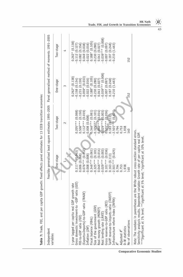
Second, we exclude those years when most transition economies inthe CEEB region experienced negative growth. By 1995 the transitionrecession largely ended in the region except in Macedonia. Therefore,we re-estimate the model for the period 1995–2005. The results arepresented in columns 2–3 of Table 7. As we can see, the effect of GDI issimilar in magnitude as before, though it is now significant at the 5%level. TRADE is significant at a 1% level and the magnitude of its effect islarger. Under the two-stage estimation, these effects are even larger inmagnitude and stronger in statistical significance. The most interestingresult is that although the FDI coefficient is positive and not statisticallysignificant under the single-stage FGLS method, it is not only positive butalso highly significant under the two-stage estimation method. The effectsof fiscal balance, size of the government, real money growth, and reallending rate are still significant and have the same signs as before. However,foreign exchange reserves now have a significant positive effect but theeffect of tariff is no longer statistically significant. Infrastructure, on theother hand, has a statistically significant negative effect, which is puzzling. Itmay be correlated with one of the variables of interest. Only an estimationof the model without TRADE makes the estimated coefficient of INFRApositive, though statistically insignificant. Thus, trade and infrastructureindex may be correlated.

Third, since N is small in our case, we estimate the dynamic version ofthe model using the generalised method of moments as suggested by Arellanoand Bond (1991). This method exploits the orthogonality conditions that existbetween lagged values of the dependent variable and the disturbances tointroduce the lagged values as instruments. We estimate the model indifferences, with lags of the dependent variable from lag 2 and above, and all


42


Author

Copy

Table

7:

Trad

e,FD

I,an

dper

capit

aGDP

gro

wth

:fi

xed

effe

cts

pan

eles

tim

ates

for

13

CEEB

tran

siti

on

econom

ies

Inde

pen

dent

variab

les

Feas

ible

gener

alis

edle

ast

squa

rees

tim

ates

1995–

2005

Panel

gener

alis

edm

ethod

ofm

om

ents

1991–

2005

One-

stag

eTw

o-st

age

One-

stag

eTw

o-s

tage

12

34

1-y

ear

lagge

dper

capit

are

alGDP

gro

wth

rate

0.2

62*

(0.1

38)

0.2

62*

(0.1

38)

Gro

ssdo

mes

tic

inve

stm

ent-

to–GDP

rati

o(G

DI)

0.1

11**

(0.0

43)

0.2

05*

**

(0.0

68)

�0.1

58

(0.1

34)

�0.1

12

(0.1

27)

FDI-

to-G

DP

rati

o(F

DI)

0.0

06

(0.0

68)

0.5

06*

**

(0.1

50)

�0.2

31

(0.1

59)

�0.0

82

(0.1

56)

(Exp

ort

s+Im

port

s)-t

o-G

DP

rati

o(T

RADE)

0.0

76***

(0.0

12)

0.1

12*

**

(0.0

19)

0.0

59*

(0.0

33)

0.0

49

(0.0

38)

Inflat

ion

(INF)

�0.0

08

(0.0

08)

�0.0

08

(0.0

08)

�0.0

22

(0.0

16)

�0.0

22

(0.0

16)

Fisc

albal

ance

(FBAL)

0.3

46***

(0.0

61)

0.3

46*

**

(0.0

61)

0.1

88*

(0.1

05)

0.1

88*

(0.1

05)

Size

ofth

ego

vern

men

t(G

OV)

�0.3

25***

(0.1

01)

�0.3

25*

**

(0.1

01)

�0.2

30

(0.2

80)

�0.2

30

(0.2

80)

Rea

lm

oney

gro

wth

(MONEY

)0.0

46***

(0.0

14)

0.0

46*

**

(0.0

14)

0.0

41

(0.0

27)

0.0

41

(0.0

27)

Rea

lle

ndin

gra

te(L

RAT

E)�

0.0

29***

(0.0

03)

�0.0

29*

**

(0.0

03)

�0.0

39*

**

(0.0

08)

�0.0

39***

(0.0

08)

Gro

ssre

serv

es-t

o-G

DP

rati

o(R

ES)

0.1

01***

(0.0

36)

0.1

01*

**

(0.0

36)

�0.0

07

(0.0

97)

�0.0

07

(0.0

97)

Tari

ffre

venue-

to-i

mport

sra

tio

(TARIF

F)0.1

63

(0.1

13)

0.1

63

(0.1

13)

0.1

97

(0.2

48)

0.1

97

(0.2

48)

Infr

astr

uctu

rere

form

inde

x(I

NFR

A)

�2.5

01***

(0.6

25)

�2.5

01*

**

(0.6

25)

�0.2

10

(1.4

63)

�0.2

10

(1.4

63)

R2

0.7

94

0.7

94

Adju

sted

R2

0.7

53

0.7

53

D–W

stat

isti

cs1.9

38

1.9

38

No

ofobse

rvat

ions

140

140

152

152

Not

e:Th

enum

ber

sin

par

enth

eses

are

the

Whit

ero

bust

cros

s-se

ctio

nst

anda

rder

rors

.Se

nsi

tivi

tyan

alys

isre

sult

s.Dep

ende

nt

variab

le:

Gro

wth

rate

ofper

capit

are

alGDP.

***Si

gnif

ican

tat

1%

leve

l;**si

gnif

ican

tat

5%

leve

l;*si

gnif

ican

tat

10%

leve

l.


43


Author

Copy

explanatory variables as instruments.21 The results are reported in columns3–4 of Table 7. The trade coefficient is statistically significant at a 10% level ofsignificance under the single-stage method, and the magnitude of theestimated coefficient is comparable to the one under single-stage FGLS.Estimated coefficients for both GDI and FDI are negative but not statisticallysignificant. The estimated coefficients of the control variables have the samesigns as the FGLS estimates except for RES, which now becomes negative butstatistically not significant. Also, only for fiscal balance and real lending rateare the coefficients statistically significant. The AR(1) coefficient is positiveand statistically significant at the 10% level.22

To summarise, our results indicate that the significant positive effect oftrade on growth is a robust empirical result for transition economies of theCEEB region. Domestic investment, too, appears to be an importantdeterminant of growth. FDI does not have any significant effect on growthwhen we consider the entire sample period. However, when we control forthe effects of domestic investment and trade on FDI, it appears to havesignificant positive effects on growth after 1995. Among other findings,macroeconomic stabilisation through fiscal and monetary policies as reflectedin fiscal balance, size of the government, and real money growth play asignificant role. That real lending rate turns out to be an importantdeterminant of growth underlines the importance of the development of thefinancial sector in transition economies.

These results have important policy implications for the transitioneconomies of the CEEB region. They are even more significant as most ofthese countries have recently joined the European Union. With free mobilityof factors of production and liberal trade policies these countries are expectedto achieve high growth.

21 Under the assumption that the regressors are strictly exogenous. See Baltagi (2002, pp. 139).22 We do conduct some additional experiments, the results of which are not reported. For

example, although we choose our model based on formal tests for exclusion of control variables,

some of the included variables may intuitively affect each other or may affect one of our variables of

interest. For example, real money growth may have an effect on real lending rate through its effects

in the money market. Similarly, tariff that reflects trade liberalisation policy may have an impact on

the trade variable. Gross reserves may also affect trade by alleviating the foreign exchange

constraint. Size of the government may have a negative impact on fiscal balance. Finally,

infrastructure may have a positive impact on FDI and trade. Therefore, in a series of experiments, we

exclude one control variable at a time from the benchmark equation and re-estimate the model. The

main conclusions are that GDI and TRADE are significant determinants of growth. Under none of

these alternative specifications, the estimated coefficient for FDI turns out to be significant when full

sample is used. Because the main results do not change, we do not report the results, and thereby

save space.


44


Author

Copy

CONCLUDING REMARKS

This paper examines the effects of trade and FDI on growth using data for 13transition economies in the CEEB region. An extension of traditional growththeory that includes trade and FDI as additional determinants of growthprovides the motivation for this study, which tries to understand growth andits sustainability in the transition economies. The transition countries of theCEEB region have witnessed a substantial increase in trade and FDI duringthe first decade of their transition from plan to market. Applying fixed effectspanel estimation methods to a data set for 1991–2005, this paper finds that asignificant positive effect of trade on growth is a robust result for thesetransition economies. Domestic investment appears to be an importantdeterminant of growth. In general, FDI does not have any significant impacton growth in transition economies. However, when we control for the effectsof domestic investment and trade on FDI, it appears to be a significantdeterminant of growth for the period after 1995. Among other findings,macroeconomic stabilisation through fiscal and monetary policies as reflectedin fiscal balance, size of the government, and real money growth play asignificant role. That real lending rate turns out to be an importantdeterminant of growth underlines the importance of the development of thefinancial sector in transition economies.

Acknowledgements

Earlier versions of this paper were presented at the 51st Annual NorthAmerican Meetings of the Regional Science Association International inSeattle, 11–13 November 2004 and at the 80th Annual Conference of theWestern Economic Association International in San Francisco, 4–8 July 2005.I thank Josef Brada, Don Bumpass, Don Freeman, Ioan Voicu, and twoanonymous referees for their insightful comments, and to Gabi Eissa,Dhrubajyoti Nath, and Rhitwik Patowary for their excellent researchassistance. Usual disclaimer applies.

REFERENCES

Anderson, TW and Hsiao, C. 1981: Estimation of dynamic models with error components. Journal of

the American Statistical Association 76: 598–606.

Antras, P and Helpman, E. 2004: Global sourcing. Journal of Political Economy 112(3): 552–580.

Arellano, M. 1989: A note on the Anderson-Hsiao estimator for panel data. Economics Letters 31:

337–341.

Arellano, M and Bond, S. 1991: Some tests of specification for panel data: Monte Carlo evidence and

an application to employment equations. Review of Economic Studies 58: 277–297.

Balasubramanyam, VN, Salisu, M and Sapsford, D. 1996: Foreign direct investment and growth in

EP and IS countries. Economic Journal 106: 92–105.


45


Author

Copy

Baltagi, BH. 2002: Econometric analysis of panel data, 2nd Edition. John Wiley & Sons Ltd.:

Chichester, UK.

Barro, RJ. 1991: Economic growth in a cross section of countries. Quarterly Journal of Economics

106(2): 407–443.

Berg, A, Borensztein, E, Sahay, R and Zettelmeyer, J. 1999: The evolution of output in transition

economies: Explaining the differences. IMF Working Paper (WP/99/73). International Monetary

Fund: Washington, DC.

Bhagwati, JN. 1973: The theory of immiserizing growth: further application. In: Connolly, MB and

Swoboda, AK (eds) International Trade and Money. University of Toronto Press: Toronto.

Borensztein, E, De Gregorio, J and Lee, J-W. 1998: How does foreign direct investment affect

economic growth? Journal of International Economics 45: 115–135.

Campos, NF and Kinoshita, Y. 2003: Why does FDI go where it goes? New evidence from transition

economies. IMF Working Paper (WP/03/228). International Monetary Fund: Washington, DC.

Cernat, L and Vranceanu, R. 2002: Globalisation and development: New evidence from central and

Eastern Europe. Comparative Economic Studies XLIV(4): 119–136.

Coe, DT and Helpman, E. 1995: International R&D spillovers. European Economic Review 39:

859–887.

de Melo, M, Denizer, C and Gelb, A. 1996: From plan to market: Patterns of transition. World Bank

Policy Research Working Paper 1564. World Bank: Washington, DC.

de Melo, M, Denizer, C, Gelb, A and Tenev, S. 1997: Circumstance and choice: The role of initial

conditions and policies in transition economies. World Bank Policy Research Working Paper 1866.

World Bank: Washington, DC.

European Bank for Reconstruction and Development (EBRD) Transition Reports. Various issues

between 1994–2006. EBRD: London.

Fischer, S, Sahay, R and Vegh, C. 1996a: Stabilization and growth in transition economies: The early

experience. Journal of Economic Perspective 10(2): 45–66.

Fischer, S, Sahay, R and Vegh, C. 1996b: Economies in transition: The beginnings of growth.

American Economic Review 86(2); Papers and Proceedings of the Hundredth and Eighth

Annual Meeting of the American Economic Association San Francisco, CA, January 5–7,

pp. 229–233.

Fleming, JM. 1955: External economies and the doctrine of balanced growth. Economic Journal 65:

241–256.

Greene, WH. 1997: Econometric analysis, 3rd Edition. Prentice-Hall: New Jersey.

Grogan, L and Moers, L. 2001: Growth empirics with institutional measures for transition countries.

Economic Systems 25: 323–344.

Grossman, GM and Helpman, E. 1992: Innovation and growth: Technological competition in the

global economy. MIT Press: Boston, MA.

Havrylyshyn, O, Izvorski, I and Rooden, R van. 1998: Recovery and growth in transition economies

1990–97: A stylized regression analysis. IMF Working Paper (WP/98/141). International

Monetary Fund: Washington, DC.

Helpman, E, Melitz, MJ and Yeaple, SR. 2004: Export versus FDI with heterogeneous firms. American

Economic Review 94(1): 300–316.

Hendry, DF. 1995: Dynamic econometrics. Oxford University Press: Oxford, New York.

Hernandez-Cata, E. 1997: Growth and liberalization during transition from plan to market. IMF Staff

Papers 44(4): 405–429.Heston, A, Summers, R and Aten, B. 2006: Penn world table Version 6.2. Center for International

Comparisons of Production, Income and Prices at the University of Pennsylvania: Philadelphia,

PA.

Hirschman, AO. 1958: The Strategy of Economic Development. Yale University Press: New Haven, CT.

Im, KS, Pesaran, MH and Shin, Y. 2003: Testing for unit roots in heterogeneous panels. Journal of

Econometrics 115: 53–74.


46


Author

Copy

Islam, N. 1995: Growth empirics: A panel data approach. Quarterly Journal of Economics 110(4):

1127–1170.

Kutan, AM and Vuksic, G. 2007: Foreign direct investment and export performance: Empirical

evidence. Comparative Economic Studies 49: 430–445.

Lee, M and Tcha, MJ. 2004: The color of money: The effects of foreign direct investment on

economic growth in transition economies. Review of World Economies 140(2): 211–229.

Levin, A, Lin, CF and Chu, C. 2002: Unit root tests in panel data: Asymptotic and finite-sample

properties. Journal of Econometrics 108: 1–24.

McKinnon, RI. 1964: Foreign exchange constraints in economic development and efficient aid

allocation. Economic Journal 74: 388–409.

Nurkse, R. 1953: Problems of capital formation in underdeveloped countries. Oxford University Press:

Oxford.

Polanec, S. 2004: Convergence at last? Evidence from transition countries. Eastern European

Economics 42(4): 55–80.

Popov, V. 2007: Shock therapy versus gradualism reconsidered: Lessons from transition economies

after 15 years of reforms. Comparative Economic Studies 49: 1–31.

Rosenstein-Rodan, PN. 1943: Problems of industrialization of Eastern and South-Eastern Europe.

Economics Journal 53: 202–211.

Sachs, JD. 1996: The transition at mid decade. American Economic Review 86(2); Papers and

Proceedings of the Hundredth and Eighth Annual Meeting of the American Economic Association

San Francisco, CA, 5–7 January, pp. 229–233.

Saggi, K. 2002: Trade, foreign direct investment and international technology transfer: A survey.

World Bank Research Observer 17(2): 191–235.

Scitovsky, T. 1954: Two concepts of external economies. Journal of Political Economy 62: 151–153.

Sohinger, J. 2005: Growth and convergence in European transition economies: The impact of foreign

direct investment. Eastern European Economics 43(2): 73–94.

UNCTAD. Statistics on foreign direct investment http://stats.unctad.org/fdi/eng/ReportFolders/

Review/explorerp.asp.

United Nations. UN statistical database http://unstats.un.org/unsd/snaama/selectionbasicFast.asp.

APPENDIX: DESCRIPTION OF THE VARIABLES AND DATA

GROWTH: Growth rate of per capita real GDP. Calculated as 100 timesfirst log differences of per capita real GDP (1990 USD), available from UNStatistical Database. Available for the entire period 1991–2005 for allcountries.

GDI: Real gross domestic investment as a percentage of real GDP. Data onreal gross fixed capital formation are obtained from the UN StatisticalDatabase and real net FDI inflows are subtracted and the percentage shares inGDP are calculated. Data are available for all years: 1991–2005 for allcountries.

FDI: Real foreign direct investment as a percentage of real GDP. Data onnet FDI inflows at current USD are obtained from the UNCTAD. They areconverted into constant dollars by applying an implicit deflator for gross fixedinvestment. Percentage shares in real GDP are then calculated. Data are


47


Author

Copy

available since 1992 for Albania, Croatia, Estonia, Latvia, Lithuania,Macedonia, and Slovenia. For Czech Republic and Slovak Republic, dataare available only since 1993.

INF: CPI inflation. Percentage change in annual average consumer priceindex (CPI). Available from the EBRD’s Transition Reports. For Estonia,Latvia, Lithuania, and Macedonia, data are available only from 1992.

FBAL: Fiscal balance. Government budget balance as a percentage ofGDP. Available from the EBRD’s Transition Reports. For Estonia and Latvia,data are available only from 1994; for Lithuania from 1993; and forMacedonia, Romania, and Slovak Republic from 1992.

GOV: Size of the government. Real government consumption expendi-tures as a percentage share in real GDP (1990 USD). Calculated from the dataobtained from the UN Statistical Database. Data are available for all years:1991–2005 for all countries.

X: Nominal exchange rate. Natural log of nominal exchange rate asreported by the EBRD’s Transition Reports. Data are available for all years:1991–2005 for all countries.

EMP: Employment growth. Percentage growth of employment as reportedin the EBRD’s Transition Reports. Data are available for Estonia, Latvia,Lithuania, and Macedonia since 1992.

MONEY: Real money growth. Percentage changes in broad measures ofmoney (M2) are available from the EBRD’s Transition reports. The real moneygrowth rate is calculated by subtracting CPI inflation. Data are available forBulgaria, Lithuania, and Slovenia from 1992; for Albania, Czech republic, andSlovak republic from 1993; for Croatia, Estonia, and Latvia from 1994; and forMacedonia from 1996.

DOMCREDIT: Real domestic credit growth. Percentage changes inoutstanding bank credits available from the EBRD’s Transition Reports. Dataare available for Bulgaria and Slovenia from 1992; for Croatia, Czech republic,Latvia, Macedonia, and Slovak Republic from 1994; for Estonia from 1995;and for Lithuania from 1996.

LRATE: Real lending rate. Data on nominal lending rates (per annum) areavailable from the EBRD’s Transition Reports. We subtract CPI inflation toobtain real lending rates. Data are available for Croatia, Czech republic,Lithuania, Macedonia, and Slovenia from 1992; for Latvia, Romania, andSlovak Republic from 1993; and for Estonia from 1994.

RES: Gross foreign exchange reserves as a percentage share of GDP. Grossforeign exchange reserves excluding gold as a percentage of GDP are availablefrom the EBRD’s Transition Reports. Data are available for Croatia andLithuania from 1992; for Estonia, Latvia, Romania, and Slovak Republic from1993; and for Macedonia from 1995.


48


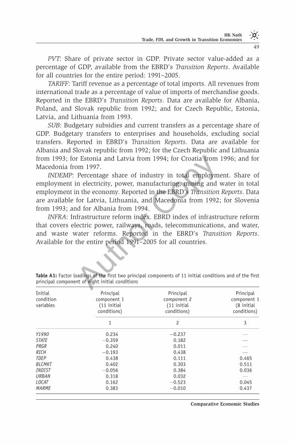
Author

Copy

PVT: Share of private sector in GDP. Private sector value-added as apercentage of GDP, available from the EBRD’s Transition Reports. Availablefor all countries for the entire period: 1991–2005.

TARIFF: Tariff revenue as a percentage of total imports. All revenues frominternational trade as a percentage of value of imports of merchandise goods.Reported in the EBRD’s Transition Reports. Data are available for Albania,Poland, and Slovak republic from 1992; and for Czech Republic, Estonia,Latvia, and Lithuania from 1993.

SUB: Budgetary subsidies and current transfers as a percentage share ofGDP. Budgetary transfers to enterprises and households, excluding socialtransfers. Reported in EBRD’s Transition Reports. Data are available forAlbania and Slovak republic from 1992; for the Czech Republic and Lithuaniafrom 1993; for Estonia and Latvia from 1994; for Croatia from 1996; and forMacedonia from 1997.

INDEMP: Percentage share of industry in total employment. Share ofemployment in electricity, power, manufacturing, mining and water in totalemployment in the economy. Reported in the EBRD’s Transition Reports. Dataare available for Latvia, Lithuania, and Macedonia from 1992; for Sloveniafrom 1993; and for Albania from 1994.

INFRA: Infrastructure reform index. EBRD index of infrastructure reformthat covers electric power, railways, roads, telecommunications, and water,and waste water reforms. Reported in the EBRD’s Transition Reports.Available for the entire period 1991–2005 for all countries.

Table A1: Factor loadings of the first two principal components of 11 initial conditions and of the firstprincipal component of eight initial conditions

Initialconditionvariables

Principalcomponent 1

(11 initialconditions)





1 2 3

Y1990 0.234 �0.237 FSTATE �0.359 0.182 FPRGR 0.240 0.011 FRICH �0.193 0.438 FTDEP 0.438 0.111 0.465BLCMKT 0.402 0.303 0.511INDIST �0.056 0.384 0.036URBAN 0.318 0.032 FLOCAT 0.162 �0.523 0.045MARME 0.383 �0.010 0.437


49


Author

Copy

REPR 0.301 0.439 0.407PLI �0.218TLI �0.339

Note: The eigenvalues corresponding to the first two principal components of 11 initial conditions are4.574 and 1.941, respectively, and these two components together explain 59.23% of variability. Theeigenvalue corresponding to the first principal component of eight initial conditions is 3.562 and thiscomponent explains 44.52% of the variability.

Table A1: (continued )

Initialconditionvariables







1 2 3


50


Documents

an important determinant of growth. In general, FDI does