The Third Round of the Euro Area Enlargement: Are the Candidates Ready?

Milan Deskar-Škrbić, Karlo Kotarac, Davor Kunovac

Zagreb, July 2019

Working Papers W-57

WORKING PAPERS W-57

PUBLISHERCroatian National Bank Publishing Department Trg hrvatskih velikana 3, 10000 Zagreb Phone: +385 1 45 64 555 Contact phone: +385 1 45 65 006 Fax: +385 1 45 64 687

WEBSITEwww.hnb.hr

EDITOR-IN-CHIEFLjubinko Jankov

EDITORIAL BOARDVedran Šošić Gordi Sušić Davor Kunovac Tomislav Ridzak Evan Kraft Maroje Lang Ante Žigman

EDITORRomana Sinković

The views expressed in this paper are not necessarily the views of the Croatian National Bank.Those using data from this publication are requested to cite the source.Any additional corrections that might be required will be made in the website version.

ISSN 1334-0131 (online)

Zagreb, July 2019

WORKING PAPERS W-57

The Third Round of the Euro Area Enlargement: Are the Candidates Ready?

Milan Deskar-Škrbić, Karlo Kotarac, Davor Kunovac

The Third Round of the Euro Area Enlargement: Are the

Candidates Ready? ∗

Milan Deskar-Škrbic, Karlo Kotarac, Davor Kunovac

Modelling Department, Croatian National Bank

July 1, 2019

Abstract

In this paper, we study the readiness of Bulgaria, Croatia and Romania to adopt

the common monetary policy of the ECB in the context of the third round of euro area

enlargement. Following the later stages of the optimal currency area (OCA) theory we

focus on the coherence of economic shocks between candidate countries and the euro

area and analyse the relevance of euro area shocks for key macroeconomic variables in

these countries. Our results, based on a novel empirical approach, show that the overall

importance of those shocks that are relevant for the ECB is fairly similar in candidate

countries and the euro area. The cost of joining the euro area should, therefore, not be

pronounced, at least from the aspect of the adoption of the common counter-cyclical

monetary policy. This conclusion holds for all three candidates, despite important

differences in monetary and exchange rate regimes.

JEL classification : E32, E52, F45

Keywords: euro area enlargement, economic shocks, BVAR, common monetary pol-

icy, Mundellian trilemma

∗Authors want to thank Ljubinko Jankov, Alan Bobetko, Marina Kunovac, Maja Bukovšak, Enes Ðo-zovic, Nina Pavic, Ozana Nadoveza Jelic, Katarina Ott, Jan Bruha and Martin Feldkircher for useful com-ments and suggestions. Also, authors want to thank participants of the Economic workshop in CroatianNational Bank, participants of the 13th International Conference "Challenges of Europe" and participantsof the 25th Dubrovnik Economic Conference for additional useful comments and suggestions.

1 Introduction

Euro area enlargement is an ongoing process. After the first eleven countries adopted the

euro in 1999 and Greece joined the euro area in 2001, the second round of enlargement

started with Slovenia in 2007 and ended with the euro adoption in Lithuania in 2015.

Today, the euro area comprises nineteen countries, with more than 340 million people and

contributes around sixteen percent to total world output.

On the twentieth anniversary of the euro, EU offi cials intensified discussion on the

third round of the enlargement as Bulgaria, Croatia and Romania started preparations to

join the Exchange Rate Mechanism (ERM II) and the euro area in the near future. The

ERM II is sometimes referred to as a euro waiting room, in which candidate countries

have to prove their ability to maintain macroeconomic and fiscal stability for at least two

years prior to joining the euro area. Croatia adopted the Strategy for euro adoption in 2017

(Eurostrategy, 2017), Bulgaria sent a letter on ERM II participation in 2018 and Romanian

offi cials set the date for euro area membership in 2024 and organised a commission for euro

adoption. The three candidates, all small open economies1, have thus clearly expressed

their willingness to join the euro area. On the other hand, there is a lack of more formal

evidence in the literature on their (in)ability smoothly to adopt the common currency and

monetary policy of the European Central Bank (ECB).

The aim of this paper is, therefore, twofold. First, to provide a broader analytical back-

ground to the discussion on the third round of euro area enlargement in general. Second,

to address the readiness of the three candidate countries to adopt the euro and common

monetary policy of the ECB. Here, we focus on the key aspect of euro area enlargement for

the candidate countries and study the potential costs of the loss of monetary sovereignty

in these countries. More precisely, we are interested in whether the common countercycli-

cal monetary policy of the ECB is likely to be suitable for these countries once they join

the monetary union. This question is even more interesting as these countries are small

1Stylised facts on these economies are discussed in Appendix A.

1

open economies with free capital flows and they all have different exchange rate regimes.

According to the IMF classification, Bulgaria operates under the regime of currency board

(EUR), Croatia implements a stabilized arrangement with an exchange rate anchor (EUR)

and Romania pursues an inflation targeting strategy, with a (managed) floating exchange

rate (EUR).

In order to study the readiness of the three economies to adopt the common monetary

policy of the euro area, we focus on the coherence of economic shocks between the euro area

and the euro candidate countries and, therefore, build on the literature on the optimum

currency area (OCA) theory. The similarity of shocks, and policy responses to these shocks,

is almost a catch-all OCA property, or meta-property, capturing the interaction between

several other properties characterizing an optimal currency area, such as business cycle

synchronization, similarity of economic structure or flexibility and movement of factors of

production (Mongelli, 2000). For that reason we investigate the importance of those shocks

that are relevant for the ECB’s monetary policy decisions ("ECB - relevant shocks") to

macroeconomic developments in the euro candidate countries.

Common monetary policy is suitable for all members in a monetary union only if eco-

nomic shocks and their macroeconomic effects in both joining and participating countries

are suffi ciently similar. In other words, those shocks that dominantly drive the business

cycles in participating countries should also play an important role in economic develop-

ments in the candidate countries. The counter-cyclical monetary policy of the ECB would

then successfully smooth out their business cycles. In that case, the loss of an independent

monetary policy should not cause any significant costs, at least from the aspect of the

appropriate counter-cyclical monetary policy. However, the costs related to giving up an

autonomous monetary policy may well depend on the exchange rate regime. This paper

thus formally addresses four main questions:

1. Do standard economic shocks affecting the euro area have similar effects on the three

candidate countries?

2

2. How important are shocks relevant for ECB policy-making process for the three

candidate countries?

3. Do monetary policy shocks of the ECB have the expected counter-cyclical effects on

the euro candidate countries?

4. Does the exchange rate regime matter for the transmission of euro area shocks to the

candidate countries?

To address these questions we rely on a structural Bayesian VAR (BVAR) model.

Several domestic and euro area structural shocks are identified by imposing a large number

of rather uncontroversial short run and long run sign and zero restrictions. Such a model,

if suffi ciently rich, is suitable to assess the relative importance of domestic and euro area

shocks for the candidate countries and therefore to address the readiness of these countries

to adopt the common monetary policy of the ECB.

The main finding of our paper is that euro area (rather than country-specific) shocks

play a dominant role in the fluctuations of output and consumer inflation in Bulgaria,

Croatia and Romania. Such results indicate that the common monetary policy could be

suitable for these countries once they adopt the euro. However there are some differences

among the three countries. The contribution of common shocks to GDP and inflation

is stronger and more similar to the euro area in Bulgaria and Croatia than in Romania.

This can, at least partially, be attributed to the fact that Romania is the only country

among the three that operates under a floating exchange rate regime. However, the con-

tribution of euro area shocks to developments of macroeconomic variables in Romania is

far from negligible, suggesting that the cost of the loss of monetary sovereignty could be

less pronounced than the standard Mundellian trilemma theory suggests. Regarding the

macroeconomic effects of the ECB policy shock, our results show that the effects of mone-

tary policy shocks in Bulgaria, Croatia and Romania are similar to those in the euro area,

which additionally supports the view that the common monetary policy can be suitable

3

for these countries. Finally, although the main focus of our paper is clearly on the three

candidate countries, in order to position our results in a broader context we compare their

similarities with the euro area to those of the other non-euro area EU members - Czechia,

Denmark, Hungary, Poland, Sweden and the UK. Our results support the view that all the

countries under analysis share a large amount of common shocks with the euro area. The

contribution of common shocks to the developments of both GDP and inflation is however

less pronounced in those with floating exchange rate regimes, which supports the view that

floating exchange rates can act as shock absorbers in most of these countries (Farant and

Peersman, 2006; Artis and Ehrmann, 2006; Audzei and Bradzik, 2018).

This paper contributes to related literature along several directions. Most importantly,

this is the first in-depth analysis of the readiness of the three candidate countries to adopt

the common ECB monetary policy in the context of the third round of euro area enlarge-

ment. Secondly, instead of only comparing the correlations of shocks (as in e.g. Bayoumi

and Eichengreen 1992, 1993 and 1994) or considering the relative importance of the euro

area shocks for candidate countries (e.g. Mackowiak, 2006; Peersman 2011; Hanclova,

2012) we propose a methodology based on historical decomposition to directly compare

the overall importance of shocks relevant for ECB policy decisions for macroeconomic vari-

ables in the candidate countries and the euro area. Focusing on the results of historical

decomposition, and not only the correlation of structural shocks, we take into account the

importance of the transmission mechanisms of structural shocks to the economy. Regard-

ing our identification scheme, in contrast to related literature, it is purposely rather loose

- we impose no restrictions onto how domestic variables react to euro area shocks. Such

a modelling decision to let the data speak freely makes these estimates less dependent on

the imposed restrictions and thus clearly more reliable. Finally, we also analyse whether

differences in the relevance of external shocks for non-euro EU economies can be explained

by their exchange rate regimes thus contributing to the literature on the role of exchange

rates as shock absorbers or shock propagators. However, our approach is different from

4

the standard strategy of Clarida and Gali (1994) who study the main sources of variation

in exchange rates. For each country we first estimate the relative importance of foreign

shocks for domestic macroeconomic developments and then look at how these statistics

differ across countries with different exchange rate regimes and with various degrees of

exchange rate volatility. Thus, we contribute to the literature focusing on the relation

between transmission of external shocks and exchange rate regimes (e.g. Canova, 2005;

Iossifov and Podpiera, 2012).

2 OCA theory, external shocks and exchange rate regimes

The aim of this section is to position our research questions in the broader context of

international macroeconomics and explain our choice of the methodology with which to

address these questions.

Following the literature in the later stages of OCA theory (e.g. Bayoumi and Einhen-

green 1992, 1993, 1994; Frankel and Rose 1997, Mongelli 2002), in this paper we emphasize

the importance of the coherence of economic shocks in the context of the loss of the au-

tonomous monetary policy as the most important cost of euro adoption for joining countries

(Eudey 1998). OCA theory postulates that this cost should not be pronounced provided

economic shocks within the monetary union are suffi ciently coherent. This is because the

coherence of economic shocks can be seen as a "catch-all" property of OCA (Mongelli,

2002) as it captures the interaction between several OCA properties, such as business cycle

synchronisation, mobility of factors of production, similarity of economic structures and

so on. Thus, coherence of economic shocks suggests that common monetary policy could

be suitable for all countries in the monetary union. In addition, OCA theory posits that

the cost of losing monetary policy autonomy is low for those countries in which economic

activity is mostly driven by the same shocks driving economic developments in the mon-

etary union. For example, if a euro candidate country is predominantly affected by the

same economic shocks as the euro area and if these shocks affect the two economies in

5

a similar fashion, the common monetary policy can then be adequate for all countries.

On the other hand, if economic activity in a joining country is predominantly driven by

some country-specific shocks, a common monetary policy could be less effective or even

counter-productive.

To take these considerations into account we need to be able to isolate domestic (idio-

syncratic) shocks from those generated abroad (in a monetary union or globally). Those

external shocks are of special interest for this analysis - these are the shocks that the ECB

generally reacts to and calibrates its monetary policy accordingly, i.e. ECB - relevant

shocks. We rely on a structural BVAR to study the importance of these shocks for the

three candidate countries. First, we study how these shocks affect the candidate countries.

If they are also important for their economies we may label them as “common shocks”.

Once we have the common shocks identified, we compare the overall importance of these

shocks for candidate countries to that for the euro area. If the same economic shocks

drive both economies in a similar way, we conclude that common monetary policy could

be suitable for both countries, just as OCA theory suggests.

By focusing on the relevance of external shocks we also complement the literature that

investigates the role of external shocks for economic dynamics in small open European

economies, still outside the euro area. Results in this strand of literature mostly suggest

that euro area shocks play important roles in economic activity in countries like Czechia,

Hungary, Poland and Slovakia (Mackowiak, 2006; Horváth and Rusnák, 2009; Hanclova,

2012) and that the cost of euro adoption would not be pronounced in these countries

(Mackowiak, 2006). In this paper we join this discussion but take a step further by asking

whether differences in the contribution of external shocks to domestic economies among

non-euro area countries can be explained by their different exchange rate regimes.

This leads us to the old debate on the characteristics of fixed vs flexible exchange

rate regimes (McKinnon 1963; Giersch 1973; Ishiyama 1975). This literature views fixed

exchange rates as direct propagators of external shocks to small open economies, while

6

flexible exchange rates can serve as shock absorbers. The standard approach to the ex-

amination of the characteristics of exchange rates as shock absorbers or shock propagators

is based on structural decomposition of exchange rate developments on contributions of

real shocks and nominal shocks (Clarida and Gali, 1994; for CEE Audzei and Bradzik,

2018). Although our model allows us to follow this strand of literature, in this paper we

take a different approach and compare the contributions of common shocks in Bulgaria

and Croatia to those in Romania and study whether the contribution of common shocks is

more pronounced in the former countries (a pegger and a quasi-pegger) than in the latter

(a floater). To give more rigor to our conclusions we expand the analysis to some other

non-euro area peggers (Denmark) and floaters (Czechia, Hungary, Poland, Sweden and the

UK) and analyse whether there is a link between variability of the nominal exchange rate

and contribution of common shocks to GDP and inflation. For example, Iossifov and Pod-

piera (2012) showed that spillovers of euro area inflation are more pronounced in non-euro

area countries with more rigid exchange rate regimes.

This literature is also closely related to the Mundellian trilemma that posits that choice

of floating exchange rate regime, under free capital flows, allows the country to run an au-

tonomous monetary policy (Obstfeld, Shambaugh and Taylor 2005). However, this propo-

sition can be misleading if external shocks play an important role in the economy of the

floater. As Gosczek and Mycielska (2019) put it, full monetary policy autonomy in coun-

tries with floating regimes can be limited by exogenous factors, primarily global interest

rates (the fear-of-float argument) or by endogenous factors, such as strong trade and fi-

nancial integration and business cycle synchronization, which amplify the importance of

external shocks in small open economies. Thus we interpret our results through the lenses

of this challenging view for the Mundellian trilemma on a global level (Aizenman, Chinn

and Ito, 2016; Rey 2016) and European level (Gosczek and Mycielska, 2019).

Finally, after the analysis of the overall contribution of external shocks to GDP and

inflation in candidate countries, we also focus on the macroeconomic effects of one partic-

7

ularly interesting shock for our analysis - ECB monetary policy shock. Thus, in this sense

we also follow growing literature on the international transmission of the ECB monetary

policy shocks that points to notable spillovers of monetary policy shocks from the euro area

to non-euro area economies (e.g. Feldkircher, 2015; Potjagailo 2017 and Colabella 2019).

3 Methodology

In this section we briefly introduce the structural VAR we rely on throughout the analysis.

We also discuss the short run and long run sign and zero restrictions we impose in order

to identify structural shocks.

3.1 Model - Structural BVAR for a small open economy

3.1.1 Basic facts on Structural VARs

General SVAR with k lags we use can be written in usual form:

A0yt = µ+A1yt−1 + . . .+Akyt−k + εt, t = 1, . . . , T. (1)

where yt is an n×1 vector of observed variables, the Aj are fixed n×n coeffi cient matrices

with invertible A0, µ is n× 1 fixed vector and εt are structural economic shocks with zero

mean and covariance matrix In. Reduced form VAR model is obtained from (1) by pre

multiplying the equation by (A0)−1 :

yt = c+B1yt−1 + . . .+Bkyt−k + ut, t = 1, . . . , T, (2)

where Bj = A−10 Aj , c = A−10 µ and ut = A−10 εt.

Structural vector autoregression (SVAR) model is normally used to calculate the impulse

response function:2

2See Killian and Lütkepohl (2017) for more details about SVARs.

8

Ψh =∂yt+h∂εt

, h = 0, 1, 2, . . .

where element ψjk,h represents average response of variable j to shock k after h periods.

The historical decomposition in a SVAR decomposes each endogenous variable in a model

into contribution of each identified shocks. The contribution of shock k to variable j at

period t and can be calculated as:

ykjt =t−1∑h=0

ψjk,h · εk,t−h. (3)

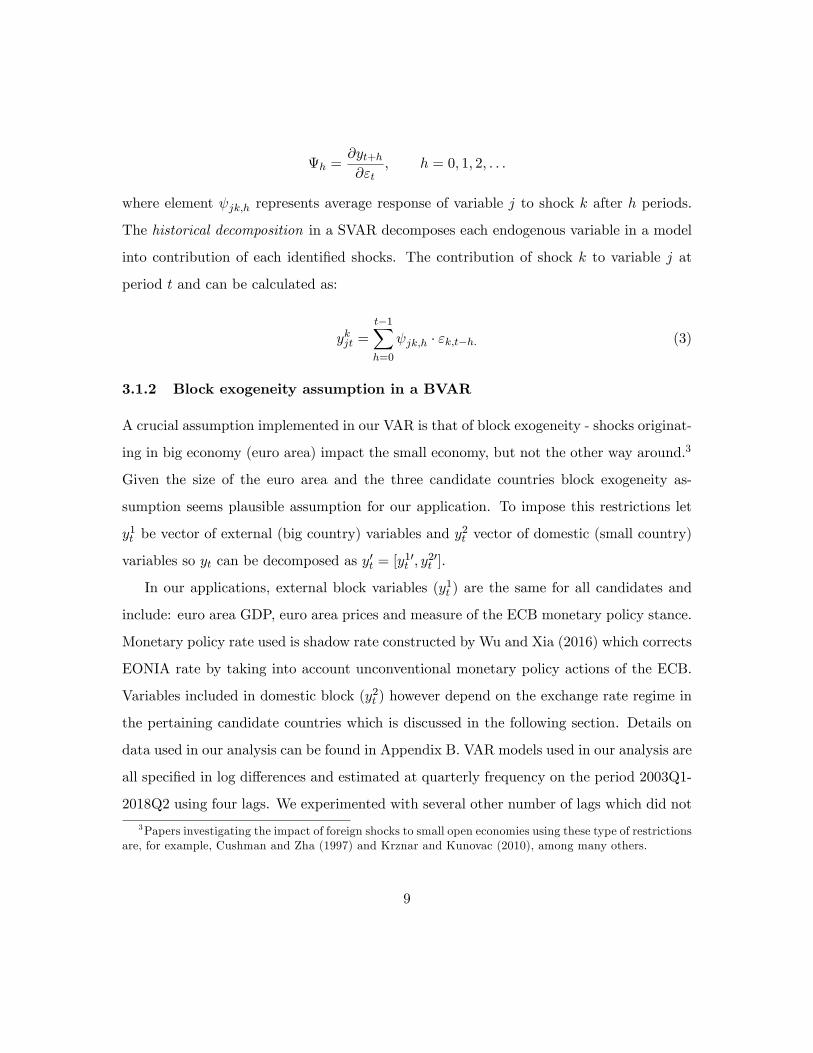
3.1.2 Block exogeneity assumption in a BVAR

A crucial assumption implemented in our VAR is that of block exogeneity - shocks originat-

ing in big economy (euro area) impact the small economy, but not the other way around.3

Given the size of the euro area and the three candidate countries block exogeneity as-

sumption seems plausible assumption for our application. To impose this restrictions let

y1t be vector of external (big country) variables and y2t vector of domestic (small country)

variables so yt can be decomposed as y′t = [y1′t , y2′t ].

In our applications, external block variables (y1t ) are the same for all candidates and

include: euro area GDP, euro area prices and measure of the ECB monetary policy stance.

Monetary policy rate used is shadow rate constructed by Wu and Xia (2016) which corrects

EONIA rate by taking into account unconventional monetary policy actions of the ECB.

Variables included in domestic block (y2t ) however depend on the exchange rate regime in

the pertaining candidate countries which is discussed in the following section. Details on

data used in our analysis can be found in Appendix B. VAR models used in our analysis are

all specified in log differences and estimated at quarterly frequency on the period 2003Q1-

2018Q2 using four lags. We experimented with several other number of lags which did not

3Papers investigating the impact of foreign shocks to small open economies using these type of restrictionsare, for example, Cushman and Zha (1997) and Krznar and Kunovac (2010), among many others.

9

change our results importantly.

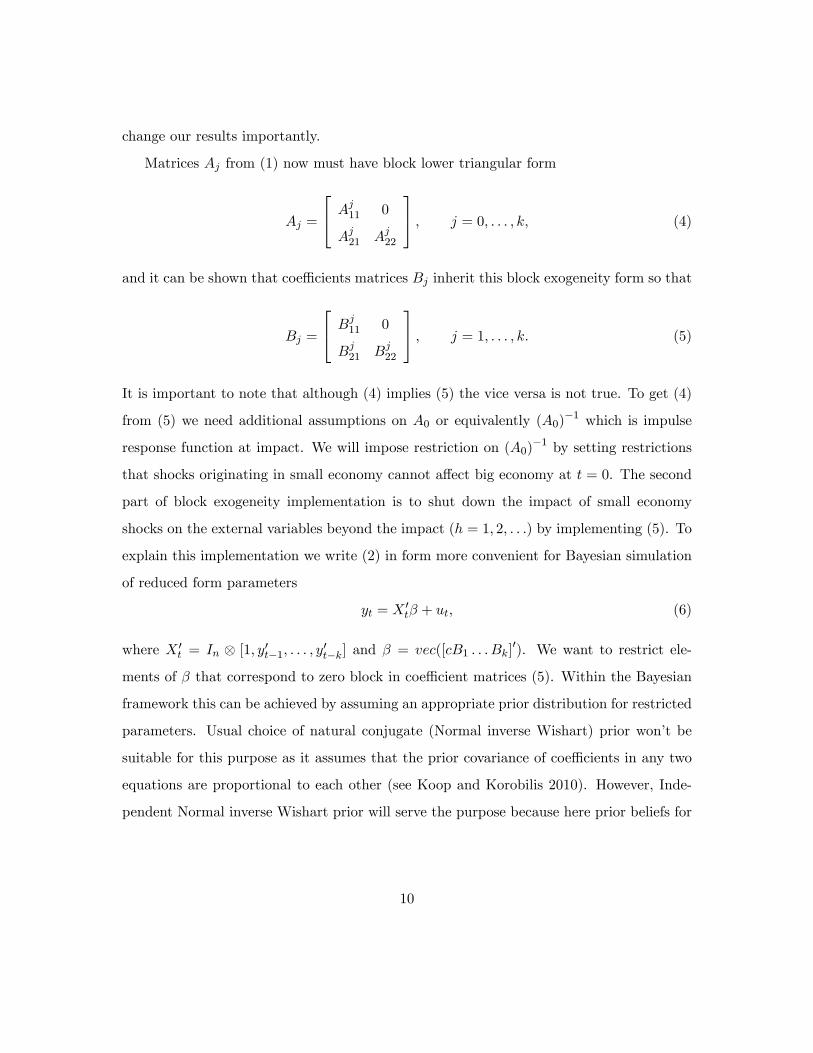
Matrices Aj from (1) now must have block lower triangular form

Aj =

Aj11 0

Aj21 Aj22

, j = 0, . . . , k, (4)

and it can be shown that coeffi cients matrices Bj inherit this block exogeneity form so that

Bj =

Bj11 0

Bj21 Bj

22

, j = 1, . . . , k. (5)

It is important to note that although (4) implies (5) the vice versa is not true. To get (4)

from (5) we need additional assumptions on A0 or equivalently (A0)−1 which is impulse

response function at impact. We will impose restriction on (A0)−1 by setting restrictions

that shocks originating in small economy cannot affect big economy at t = 0. The second

part of block exogeneity implementation is to shut down the impact of small economy

shocks on the external variables beyond the impact (h = 1, 2, . . .) by implementing (5). To

explain this implementation we write (2) in form more convenient for Bayesian simulation

of reduced form parameters

yt = X ′tβ + ut, (6)

where X ′t = In ⊗ [1, y′t−1, . . . , y′t−k] and β = vec([cB1 . . . Bk]

′). We want to restrict ele-

ments of β that correspond to zero block in coeffi cient matrices (5). Within the Bayesian

framework this can be achieved by assuming an appropriate prior distribution for restricted

parameters. Usual choice of natural conjugate (Normal inverse Wishart) prior won’t be

suitable for this purpose as it assumes that the prior covariance of coeffi cients in any two

equations are proportional to each other (see Koop and Korobilis 2010). However, Inde-

pendent Normal inverse Wishart prior will serve the purpose because here prior beliefs for

10

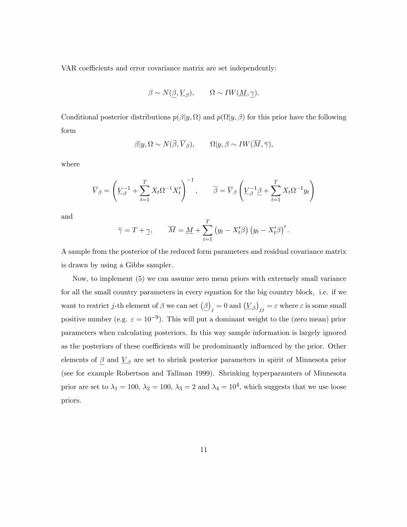
VAR coeffi cients and error covariance matrix are set independently:

β ∼ N(β, V β), Ω ∼ IW (M,γ).

Conditional posterior distributions p(β|y,Ω) and p(Ω|y, β) for this prior have the following

form

β|y,Ω ∼ N(β, V β), Ω|y, β ∼ IW (M,γ),

where

V β =

(V −1β +

T∑t=1

XtΩ−1X ′t

)−1, β = V β

(V −1β β +

T∑t=1

XtΩ−1yt

)

and

γ = T + γ, M = M +

T∑t=1

(yt −X ′tβ

) (yt −X ′tβ

)′.

A sample from the posterior of the reduced form parameters and residual covariance matrix

is drawn by using a Gibbs sampler.

Now, to implement (5) we can assume zero mean priors with extremely small variance

for all the small country parameters in every equation for the big country block, i.e. if we

want to restrict j-th element of β we can set(β)j

= 0 and(V β

)jj

= ε where ε is some small

positive number (e.g. ε = 10−9). This will put a dominant weight to the (zero mean) prior

parameters when calculating posteriors. In this way sample information is largely ignored

as the posteriors of these coeffi cients will be predominantly influenced by the prior. Other

elements of β and V β are set to shrink posterior parameters in spirit of Minnesota prior

(see for example Robertson and Tallman 1999). Shrinking hyperparamters of Minnesota

prior are set to λ1 = 100, λ2 = 100, λ3 = 2 and λ4 = 104, which suggests that we use loose

priors.

11

3.1.3 Set-identification of structural shocks

At each step of our Gibbs sampler, given a draw of reduced form parameters, we recover a

set of structural models satisfying the sign and zero restrictions imposed. The sign and zero

restrictions are imposed directly onto the impulse response function by using a procedure

proposed by Arias et al. (2014.). This algorithm may be effi ciently implemented in our

application where both the block exogeneity assumption and standard sign restrictions

are to be imposed. Arias et al (2018) also propose the updated version of the algorithm,

but now fully specified under a normal inverse Wishart prior only. As such, it cannot

be adjusted easily to accommodate the block exogeneity assumption - a feature of the

highest importance when modelling interactions between a small open economy and the

rest of the world. For that reason we rely on the procedure proposed by Arias et al.

(2014.) instead. In order to test whether the choice of the algorithm version (Arias et

al. (2014.) or Arias et al (2018)) affects our results we ran several specifications, without

block exogeneity assumption, and compared the output from the two specifications. The

results would always be almost identical, suggesting that the choice of the algorithm is not

of great importance in this case.4

4 Identification with sign and zero restrictions

Structural shocks are identified by imposing a number of sign and zero restrictions on the

impulse response function in the short run and the long run. Identification strategy is

largely based on the mainstream macroeconomic theory and the recent related literature

(see for example Forbes et al. 2018, Bobeica and Jarocinski 2017 and Comunale and

Kunovac 2017). Each shock belongs to one of the two main groups: external or domestic

(country specific) shocks. External shocks by definition (i.e. imposed restrictions) affect

the euro area. They may originate either in the euro area or globally (oil supply or global

4These are available upon request.

12

demand for example). For our purpose it is important only that these shocks affect the

euro area and are thus relevant for the ECB - we label them jointly euro area shocks. On

the other hand, domestic shocks are country specific and are identified by imposing block

exogeneity restrictions together with sign and zero restrictions. We impose no restrictions

on how domestic variables react to euro area shocks and thus let the data speak freely in

that regard. If, however, domestic variables do react to external shocks in a way similar to

the those of the euro area we may also correctly label the external shocks common shocks.

Identified euro area shocks are labelled the aggregate demand, aggregate supply and

monetary policy shocks. In the short run, an expansionary aggregate demand shock in-

creases both economic activity and prices in the euro area. Monetary policy then acts

counter-cyclically and raises the policy rate. In contrast, an aggregate supply shock has

the opposite effect on economic activity and prices in euro area - it raises GDP and low-

ers consumer inflation, while there reaction of monetary policy here is left unrestricted.

Finally, an expansionary monetary policy shock increases both economic activity and in-

flation. As for the long run restrictions, we assume that aggregate demand and monetary

policy shocks do not affect GDP in the long run.

For each of the three candidate countries we also identify several domestic shocks,

depending on the monetary and exchange rate regime in these countries. Specifications

for Croatia and Romania, in contrast to Bulgaria, which operates under a currency board

regime, include the exchange rate 5 of the domestic currency vis-a-vis euro. Also, Romania,

in contrast to the other two candidate countries, uses reference rate as a key monetary

policy instrument and the corresponding VAR thus includes domestic interest rate. For

all countries of interest (Bulgaria, Croatia and Romania) we identify short run domestic

aggregate supply and domestic aggregate demand shocks in similar fashion as for the euro

area: correlation of economic activity and prices is positive in the case of demand shock,

5Appreciation of domestic currency is represented as decrease of exchange rate level.

13

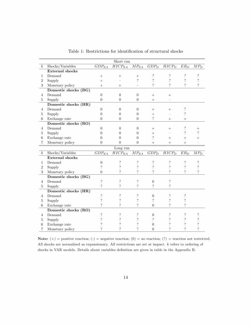
Table 1: Restrictions for identification of structural shocks

Short runk Shocks/Variables GDPEA HICPEA MPEA GDPD HICPD ERD MPD

External shocks1 Demand + + + ? ? ? ?2 Supply + — ? ? ? ? ?3 Monetary policy + + — ? ? ? ?

Domestic shocks (BG)4 Demand 0 0 0 + +5 Supply 0 0 0 + —

Domestic shocks (HR)4 Demand 0 0 0 + + ?5 Supply 0 0 0 + — ?6 Exchange rate 0 0 0 ? + +

Domestic shocks (RO)4 Demand 0 0 0 + + ? +5 Supply 0 0 0 + — ? ?6 Exchange rate 0 0 0 ? + + +7 Monetary policy 0 0 0 + + + —

Long runk Shocks/Variables GDPEA HICPEA MPEA GDPD HICPD ERD MPD

External shocks1 Demand 0 ? ? ? ? ? ?2 Supply ? ? ? ? ? ? ?3 Monetary policy 0 ? ? ? ? ? ?

Domestic shocks (BG)4 Demand ? ? ? 0 ?5 Supply ? ? ? ? ?

Domestic shocks (HR)4 Demand ? ? ? 0 ? ?5 Supply ? ? ? ? ? ?6 Exchange rate ? ? ? 0 ? ?

Domestic shocks (RO)4 Demand ? ? ? 0 ? ? ?5 Supply ? ? ? ? ? ? ?6 Exchange rate ? ? ? 0 ? ? ?7 Monetary policy ? ? ? 0 ? ? ?

Note: (+) = positive reaction; (-) = negative reaction; (0) = no reaction; (?) = reaction not restricted.

All shocks are normalized as expansionary. All restrictions are set at impact. k refers to ordering of

shocks in VAR models. Details about variables definition are given in table in the Appendix B.

14

and negative in the case of supply shock. Regarding demand shock, we assume that this

shock increases interest rate for Romania as a counter-cyclical reaction of monetary policy.

For Croatia and Romania we also identify exchange rate shock - exogenous depreciation

of domestic currency raises domestic inflation (pass-through effect) in both countries and

interest rate in Romania only. We do not impose any restrictions on the effects of domestic

demand shocks on exchange rate as the literature related to these effects is inconclusive.

6. Finally, for Romania we identify a domestic monetary policy shock similar to that in

the euro area, additionally assuming that a lower domestic interest rate depreciates the

domestic currency. A summary of our identification strategy is given in 1. As for the long

run restrictions in the domestic block, we assume that aggregate demand (BG, HR, RO),

exchange rate (HR, RO) and monetary policy (RO) shocks do not affect GDP in the long

run.

4.1 Relative and overall importance of individual shocks based on his-

torical decomposition

In this paper, importance of external shocks for domestic economies is quantified using

several statistics based on the historical decomposition from the estimated VARs presented

above. First, from historical decomposition (see (3), where ykjt represents contribution of

shock k to variable j at period t, we define measure of the relative importance (in absolute

terms) of some shock k to variable j at t as:

ykjt =

∣∣∣ykjt∣∣∣∑nl=1

∣∣∣yljt∣∣∣ . (7)

6Rising domestic demand can lead to increase of money demand and thus appreciate domestic currency.On the other hand, stronger domestic demand can widen trade deficit, which puts depreciation pressureson domestic currency. With no restrictions on the effect of domestic demand on exchange rate it is hard toseparate exchange rate shock from domestic demand shock (correlation between these shocks is pronounced).However, in our analysis we focus on the importance of external shocks and contribution of these shocks todevelopments of domestic macroeconomic variables is not affected by the structure of domestic shocks.

15

Now, our measure of the overall importance of external shocks (k = 1, 2, 3) for some

domestic macroeconomic variable j at period t is the sum of contributions of these shocks:

3∑k=1

ykjt. (8)

Second, to measure the similarity of contributions of some shock to a domestic (j) and

corresponding euro area (j′ ) variable (economic activity or prices) we look at the difference:

ykjt − ykj′t. (9)

This measure takes the value of 0 if the contribution of the given shock in the euro area

and the euro candidate country are identical, meaning that all values close to 0 indicate

the pronounced similarity of these contributions.

5 Results

In this section we present and discuss the results from the estimated structural BVARs.

First, we report the contributions of euro area shocks to GDP and inflation developments

in the three candidate countries. After that we compare these contributions to those in the

euro area. From these results, we discuss the adequacy of the common monetary policy

for the euro candidate countries through the lenses of the OCA theory and discuss the

differences among the countries through the prism of the Mundellian framework. Next,

in the context of the international monetary policy transmission, we report how the ECB

monetary policy shock affects macroeconomic variables in three candidate countries.

16

5.1 Relevance of common shocks for candidate countries and similarity

with the euro area

Impulse responses of all models together with 68% posterior error bands are given in

Appendix B (Figures 6 - 8). They broadly suggest that the three countries do react to

euro area shocks in a manner similar to that of the euro area and, thus, we may label these

shocks “common shocks”.

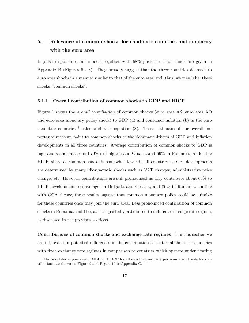
5.1.1 Overall contribution of common shocks to GDP and HICP

Figure 1 shows the overall contribution of common shocks (euro area AS, euro area AD

and euro area monetary policy shock) to GDP (a) and consumer inflation (b) in the euro

candidate countries 7 calculated with equation (8). These estimates of our overall im-

portance measure point to common shocks as the dominant drivers of GDP and inflation

developments in all three countries. Average contribution of common shocks to GDP is

high and stands at around 70% in Bulgaria and Croatia and 60% in Romania. As for the

HICP, share of common shocks is somewhat lower in all countries as CPI developments

are determined by many idiosyncratic shocks such as VAT changes, administrative price

changes etc. However, contributions are still pronounced as they contribute about 65% to

HICP developments on average, in Bulgaria and Croatia, and 50% in Romania. In line

with OCA theory, these results suggest that common monetary policy could be suitable

for these countries once they join the euro area. Less pronounced contribution of common

shocks in Romania could be, at least partially, attributed to different exchange rate regime,

as discussed in the previous sections.

Contributions of common shocks and exchange rate regimes I In this section we

are interested in potential differences in the contributions of external shocks in countries

with fixed exchange rate regimes in comparison to countries which operate under floating

7Historical decompositions of GDP and HICP for all countries and 68% posterior error bands for con-tributions are shown on Figure 9 and Figure 10 in Appendix C.

17

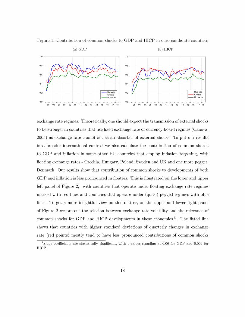
Figure 1: Contribution of common shocks to GDP and HICP in euro candidate countries

(a) GDP

0.0

0.2

0.4

0.6

0.8

1.0

05 06 07 08 09 10 11 12 13 14 15 16 17 18

BulgariaCroatiaRomania

(b) HICP

0.0

0.2

0.4

0.6

0.8

1.0

05 06 07 08 09 10 11 12 13 14 15 16 17 18

BulgariaCroatiaRomania

exchange rate regimes. Theoretically, one should expect the transmission of external shocks

to be stronger in countries that use fixed exchange rate or currency board regimes (Canova,

2005) as exchange rate cannot act as an absorber of external shocks. To put our results

in a broader international context we also calculate the contribution of common shocks

to GDP and inflation in some other EU countries that employ inflation targeting, with

floating exchange rates - Czechia, Hungary, Poland, Sweden and UK and one more pegger,

Denmark. Our results show that contribution of common shocks to developments of both

GDP and inflation is less pronounced in floaters. This is illustrated on the lower and upper

left panel of Figure 2, with countries that operate under floating exchange rate regimes

marked with red lines and countries that operate under (quasi) pegged regimes with blue

lines. To get a more insightful view on this matter, on the upper and lower right panel

of Figure 2 we present the relation between exchange rate volatility and the relevance of

common shocks for GDP and HICP developments in these economies.8. The fitted line

shows that countries with higher standard deviations of quarterly changes in exchange

rate (red points) mostly tend to have less pronounced contributions of common shocks

8Slope coeffi cients are statistically significant, with p-values standing at 0,06 for GDP and 0,004 forHICP.

18

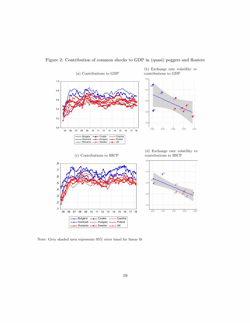
Figure 2: Contribution of common shocks to GDP in (quasi) peggers and floaters

(a) Contributions to GDP

0.0

0.2

0.4

0.6

0.8

1.0

05 06 07 08 09 10 11 12 13 14 15 16 17 18

Bulgaria Croatia CzechiaDenmark Hungary PolandRomania Sweden UK

(b) Exchange rate volatility vscontributions to GDP

BG

CZ

HR

HU

PL

ROUKDK

SW

0.4

0.5

0.6

0.7

0.8

0.00 0.01 0.02 0.03 0.04

(c) Contributions to HICP

.1

.2

.3

.4

.5

.6

.7

.8

05 06 07 08 09 10 11 12 13 14 15 16 17 18

Bulgaria Croatia CzechiaDenmark Hungary PolandRomania Sweden UK

(d) Exchange rate volatility vscontributions to HICP

BG

CZ

HR

HU

PLRO

UK

DK

SW

0.4

0.5

0.6

0.7

0.8

0.00 0.01 0.02 0.03 0.04

Note: Grey shaded area represents 95% error band for linear fit

19

to GDP9 and inflation. These conclusions are broadly consistent with views that floating

exchange rates can be seen as shock absorbers in most of these countries (Audzei and

Bradzik, 2018). However, we present the relation between exchange rate volatility and the

relevance of common shocks for GDP and HICP developments in these economies.although

the contribution of common shocks in new EU member state floaters, Poland, Hungary

and Czechia, is somewhat less pronounced in comparison to their peers with more rigid

exchange rate regimes, Bulgaria and Croatia, this contribution is far from negligible. These

findings are in line with the related literature (Mackowiak, 2006; Horváth and Rusnák, 2009;

Hanclova, 2012) and can also serve as a framework for the discussion on euro adoption in

these countries. As Poland, Hungary and Czechia are obliged by their Treaties of Accession

to the European Union to introduce the euro eventually this issue is relevant for policy

makers despite the fact that the current political atmosphere in these countries is not

pro-euro oriented. Increasing financial and trade integration of these countries with the

euro area and ongoing euro area reforms could bring this question to the top of the policy

agenda in the near future. Our results can be also interpreted in terms of global business

(e.g. Kose, Otrok and Prasad 2012; Ductor and Leiva-Leon, 2016) and financial (Rey

2016) cycles synchronization literature, which suggests that in the era of globalization

and financial internationalization common global economic and financial shocks strongly

affect economic developments and economic policy decision making process in small open

economies.

5.1.2 Contribution of individual common shocks to GDP and HICP

Previously presented results on the overall contribution of common shocks to the devel-

opments of macroeconomic variables in euro candidate countries are rather informative.9The only outlier in the sample is GDP for Denmark, as contribution of euro area shocks in this pegger

country is among the lowest in the group. This deviation can be explained by the fact that Denmarkexperienced volatile growth rates in the pre-crisis period (even with negative quarterly figures) and recordeda technical recession in 2017, due to some idiosyncratic one-offs (primarily some patent payments whichincreased volatility of the growth rate in first two quarters of the year and temporary bottlenecks in carsales due to changes in tax system in September)

20

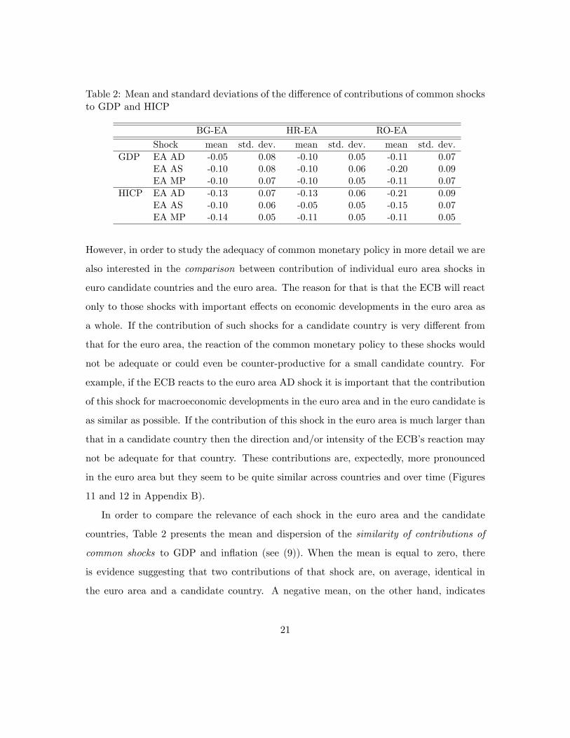
Table 2: Mean and standard deviations of the difference of contributions of common shocksto GDP and HICP

BG-EA HR-EA RO-EA

Shock mean std. dev. mean std. dev. mean std. dev.GDP EA AD -0.05 0.08 -0.10 0.05 -0.11 0.07

EA AS -0.10 0.08 -0.10 0.06 -0.20 0.09EA MP -0.10 0.07 -0.10 0.05 -0.11 0.07

HICP EA AD -0.13 0.07 -0.13 0.06 -0.21 0.09EA AS -0.10 0.06 -0.05 0.05 -0.15 0.07EA MP -0.14 0.05 -0.11 0.05 -0.11 0.05

However, in order to study the adequacy of common monetary policy in more detail we are

also interested in the comparison between contribution of individual euro area shocks in

euro candidate countries and the euro area. The reason for that is that the ECB will react

only to those shocks with important effects on economic developments in the euro area as

a whole. If the contribution of such shocks for a candidate country is very different from

that for the euro area, the reaction of the common monetary policy to these shocks would

not be adequate or could even be counter-productive for a small candidate country. For

example, if the ECB reacts to the euro area AD shock it is important that the contribution

of this shock for macroeconomic developments in the euro area and in the euro candidate is

as similar as possible. If the contribution of this shock in the euro area is much larger than

that in a candidate country then the direction and/or intensity of the ECB’s reaction may

not be adequate for that country. These contributions are, expectedly, more pronounced

in the euro area but they seem to be quite similar across countries and over time (Figures

11 and 12 in Appendix B).

In order to compare the relevance of each shock in the euro area and the candidate

countries, Table 2 presents the mean and dispersion of the similarity of contributions of

common shocks to GDP and inflation (see (9)). When the mean is equal to zero, there

is evidence suggesting that two contributions of that shock are, on average, identical in

the euro area and a candidate country. A negative mean, on the other hand, indicates

21

that contributions of common shocks are, on average, higher in the euro area than in

the candidate countries. Reported averages indicate that contributions of all shocks are,

expectedly, more pronounced in the euro area in the case of both GDP and inflation. The

contribution of common shocks to GDP is lower in the three countries compared to the euro

area - in Bulgaria and Croatia it is (on average) lower by 10pp and in Romania by 15pp.

The maximum difference is found in the case of the contribution of the common AS shock

in Romania, standing at around 20pp. As for inflation, the differences are somewhat more

pronounced, which is not surprising if we take into account various country-specific tax

and administrative price changes that directly affect inflation dynamics in these countries.

However, these differences are, in our view, still relatively modest. The contribution of

common shocks to inflation is around 12pp lower in Bulgaria, 10pp in Croatia and 14pp in

Romania than in the euro area. The maximum difference is again recorded in the case of

Romania, where the average contribution of common AD shock is 21pp lower, on average,

than in the euro area. More pronounced differences in contributions of common shocks in

the case of Romania can also be interpreted in terms of its different exchange rate regime.

In addition to average differences, we also report standard deviations which are in all cases

below 0.10, which suggests that the dynamics of contributions of common shocks in the

candidate countries and the euro area is quite similar. Figures 11 and 12 in Appendix

B show that changes in contributions of common shocks to GDP and inflation over time

in euro candidate countries and the euro area are synchronized. Thus, these results also

suggest that common monetary policy could be suitable for all countries.

5.2 Effects of the ECB’s monetary policy on macroeconomic variables in

candidate countries

In previous sections we discussed the adequacy of common monetary policy by focusing

on various aspects of the coherence of economic shocks. In this section we focus on the

monetary policy and directly compare the effects of the ECB policy actions on the euro

22

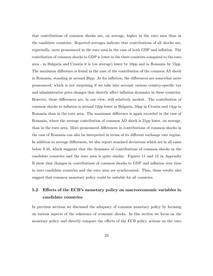
area and on the candidate countries.

Figure 3: Effects of the ECB monetary policy shock on GDP and inflation

(a) EA

5 10 15 20

-0.1

0

0.1

0.2

0.3

0.4

0.5

EA MP ==> gdp-ea

5 10 15 20

0.1

0.2

0.3

0.4

EA MP ==> hicp-ea

(b) BG

5 10 15 20

-0.6

-0.4

-0.2

0

0.2

0.4

0.6

EA MP ==> gdp-bg

5 10 15 20-0.5

0

0.5

1

EA MP ==> hicp-bg

(c) HR

5 10 15 20

-0.5

0

0.5

EA MP ==> gdp-hr

5 10 15 20

0

0.1

0.2

0.3

0.4

0.5

0.6

EA MP ==> hicp-hr

(d) RO

5 10 15 20

-0.5

0

0.5

1

EA MP ==> gdp-ro

5 10 15 200

0.5

1

1.5

EA MP ==> hicp-ro

Note: Results are represented with point-wise median and 68% confidence bands.

Figure 3 shows the estimated impulse response functions, reflecting how expansionary

ECB monetary policy shock affects the GDP and consumer inflation in the candidate coun-

tries and the euro area. Importantly, impulse responses indicate that the effect of this shock

among countries is fairly similar and our results are broadly in line with related literature

(e.g. Feldkircher, 2015; Potjagailo 2017 and Colabella 2019). The similarity of responses of

GDP and inflation in the euro area and in the euro candidate countries reflects the strong

role of the so-called trade channel in international monetary policy transmission (Potjagailo

2017; Iacoviello and Navarro 2018). An expansionary monetary policy shock has a positive

short term effect on GDP in the euro area and in euro candidate countries, while this effect

fades away and/or becomes statistically insignificant in the longer run. On the other hand,

the effects of the ECB monetary policy shock on inflation in all countries are positive and

23

long-lasting. To give our conclusions more analytical rigor, we calculated differences of

impulse responses to ECB monetary policy shock between the candidate countries and the

euro area (Figure 14 in Appendix B). In most cases responses of GDP and inflation in

candidate countries and the euro area are statistically not different. There are only two

cases in which there are statistically significant differences in responses. Firstly, there is

short lasting statistically significant difference in responses for GDP between Bulgaria and

euro area. Secondly, the reaction of HICP in Romania to EA monetary policy shock is

constantly significantly higher than the reaction of EA HICP, which can, at least partially,

be explained by the fact that in the observed period Romania recorded the highest and

most volatile inflation rates. Comparable reactions of macroeconomic variables to the ECB

monetary policy shock indicate that common counter-cyclical policy could be effective in

euro candidate economies, especially if we take into account the endogeneity hypothesis of

the OCA theory (Frankel and Rose, 1998) suggesting that similarity of economic shocks

and reactions to these shocks could become even more pronounced once the candidates

join the euro area.

5.3 Robustness of the results

In order to test the robustness of our main results on the importance of euro area shocks

for the three candidate economies, we challenge our identification pattern. Having in mind

that the historical decomposition exercise in a SVAR may depend heavily on a particular

combination of restrictions imposed onto the impulse response function, we test whether

varying the identification pattern influences our main conclusions. First, when distinguish-

ing among shocks, the most challenging part was to distinguish between the aggregate

demand and the monetary policy shock and, to some extent, also the exchange rate shock.

The pattern of sign and zero restrictions needed for that purpose may overlap, making

reliable identification of structural shocks a rather challenging task. For that purpose we

tested several alternative patterns which would indeed slightly affect the relative impor-

24

tance of those shocks on candidate countries. However, this was largely irrelevant for our

main conclusions on the overall importance of euro area shocks for the three candidates.

Domestic shocks are distinguished from those originating abroad by imposing block exo-

geneity restrictions and the overall importance of the two groups of shocks would therefore

remain largely unchanged when varying the identification pattern within each group of

shocks (domestic or external). Similarly, instead of having a single foreign block we exper-

imented with a model with distinct euro area and global blocks. However, although such

a richer structure may help to explain the sources of shocks hitting the three candidate

countries better, this has not changed our results importantly. For simplicity, but without

important loss of generality, our final specification merged both euro area and global shocks

into a single block.

6 Conclusion

Returning to the research questions posed at the beginning, the results of our empirical

approach show that economic shocks hitting the euro area have similar effects on the three

candidate countries. Our measure of similarity of contributions shows that differences in

reactions to common shocks are rather small among the three countries, but somewhat

more pronounced in Romania. At least partially, this can be explained by the fact that

during the observed period Romania recorded significantly strong variations of the ex-

change rate compared to other two countries. This view was supported by comparison of

the contributions of common shocks in Romania and other floaters in the EU - Czechia,

Hungary, Poland, Sweden and UK with (quasi) peggers Denmark, Bulgaria and Croatia.

This comparison showed that the share of common shocks in the former group of countries

is smaller than that in the latter group. However, due to strong trade and financial link-

ages within the EU, the contribution of external shocks in floaters is far from negligible.

The same therefore will hold true for Romania. For that reason, we expect that costs

of giving up monetary sovereignty could be less pronounced than standard Mundellian

25

trilemma suggests. As for the introduction of a more rigid exchange rate regime in Roma-

nia, current developments show that the Romanian National Bank is making an effort to

keep the exchange rate relatively stable, which can probably be explained by the relatively

high level of financial euroisation in the country (Copaciu, Nalban and Bulete, 2015) and

the relatively pronounced exchange rate pass through effect (Stoian and Murarasu, 2015).

Despite the evidence that the exchange rate in Romania absorbs part of the real shocks

in the economy, the absorption capacity is limited by the structural characteristics of the

economy. Regarding the other two countries, monetary policies in Bulgaria and Croatia are

already fairly limited as they operate under a currency board (Bulgaria) and a managed

float with a tight margin (Croatia) exchange rate regime. Regarding the adequacy of the

ECB’s policy for these countries, impulse responses from BVAR point to expected counter-

cyclical effects in both euro area and euro candidate countries. These results also support

the view that the costs of euro adoption, in terms of loss of an autonomous counter-cyclical

monetary policy, should be relatively modest in all three countries, especially in Bulgaria

and Croatia.

Finally, it is important to emphasize that there are various other costs of euro adoption,

which are not addressed in this paper, such as price increase due to currency conversion,

one-off conversion costs and one-off costs arising from the participation in the Eurosystem

as well as the costs of participation in the provision of financial assistance to other member

states. However, as Eudey (1998) points out, loss of an autonomous counter-cyclical mon-

etary policy can be understood as the most important long lasting cost of euro adoption,

and our results suggest that this cost would not be pronounced in the three candidate

countries.

26

References

[1] Aizenman, J., Chinn, M. D., and Ito, H. (2016). Monetary policy spillovers and the

trilemma in the new normal: Periphery country sensitivity to core country conditions.

Journal of International Money and Finance, 68, 298-330.

[2] Audzei, V., and Brázdik, F. (2018). Exchange rate dynamics and their effect on macro-

economic volatility in selected CEE countries. Economic Systems, 42(4), 584-596.

[3] Arias, J., Rubio-Ramírez, J. F., and Waggoner, D. F. (2014). Inference Based on SVAR

Identified with Sign and Zero Restrictions: Theory and Applications. International

Finance Discussion Papers 1100, Board of Governors of the Federal Reserve Syste

(U.S.)

[4] Arias, J., Rubio-Ramírez, J. F., and Waggoner, D. F. (2018.) Inference Based on

Structural Vector Autoregressions Identified With Sign and Zero Restrictions: The-

ory and Applications, Econometrica, Econometric Society, vol. 86(2), pages 685-720,

March

[5] Artis, M., and Ehrmann, M. (2006). The exchange rate—A shock-absorber or source of

shocks? A study of four open economies. Journal of International Money and Finance,

25(6), 874-893.

[6] Bayoumi T. and B. Eichengreen (1992). Shocking Aspects of European Monetary

Unification, NBER Working Paper, No. 3949.

[7] Bayoumi T. and B. Eichengreen (1993). Is there a conflict between EC enlargement

and European monetary unification, Greek Economic Review 15, No. 1, pp 131 —154

[8] Bayoumi T. and B. Eichengreen (1994). One money or many? Analysing the prospects

for monetary unification in various parts of the World, Princeton Studies in Interna-

tional Finance No. 76

27

[9] Bluwstein, K., and Canova, F. (2016). Beggar-thy-neighbor? The international effects

of ECB unconventional monetary policy measures. International Journal of Central

Banking, 12(3), 69-120.

[10] Bobeica, E. and Jarocinski, M. (2017). Missing disinflation and missing inflation: the

puzzles that aren’t, ECB Working paper series, No. 2000, January.

[11] Canova, F. (2005). The transmission of US shocks to Latin America. Journal of Applied

econometrics, 20(2), 229-251.

[12] Christiano, L. and T. Fitzgerald (2003). The band pass filter, International Economic

Review 44 (2), 435—465.

[13] Ciarlone, A., and Colabella, A. (2016). Spillovers of the ECB’s non-standard monetary

policy into CESEE economies. Ensayos sobre Política Económica, 34(81), 175-190.

[14] Clarida, R., and Gali, J. (1994). Sources of real exchange-rate fluctuations: How

important are nominal shocks?. In Carnegie-Rochester conference series on public

policy (Vol. 41, pp. 1-56). North-Holland.

[15] Comunale, M. and Kunovac, D. (2017). Exchange rate pass-through in the euro area,

ECB Working paper series, No. 2003, February.

[16] Copaciu, M., Nalban, V., and Bulete, C. (2015, November). REM 2.0-An estimated

DSGE model for Romania. In 11th Dynare Conference, Brussels, National Bank of

Belgium.

[17] Colabella, A. (2019). Do the ECB’s monetary policies benefit emerging market

economies? A GVAR analysis on the crisis and post-crisis period. Bank of Italy,

Economic Research and International Relations Area. No. 1207

28

[18] Cushman, D. O., and T. Zha (1997). Identifying monetary policy in a small open

economy under flexible exchange rates, Journal of Monetary Economics, 39(3), 433-

448.

[19] Ductor, L., and Leiva-Leon, D. (2016). Dynamics of global business cycle interdepen-

dence. Journal of International Economics, 102, 110-127.

[20] Eudey, G. (1998). Why is Europe forming a monetary union?. Business Review, (Nov),

13-21.

[21] Feldkircher, M. (2015). A global macro model for emerging Europe. Journal of Com-

parative Economics, 43(3), 706-726.

[22] Forbes, K., Hjortsoe, I., and Nenova, T. (2018). The shocks matter: improving our

estimates of exchange rate pass-through. Journal of International Economics, 114,

255-275.

[23] Frankel, J. A., and Rose, A. K. (1997). Is EMU more justifiable ex post than ex ante?.

European Economic Review, 41(3), 753-760.

[24] Frankel, J. A., and Rose, A. K. (1998). The endogenity of the optimum currency area

criteria. The Economic Journal, 108(449), 1009-1025.

[25] Giersch, H. (1973). On the desirable degree of flexibility of exchange rates. Review of

World Economics, 109(2), 191-213.

[26] Goczek, L., and Mycielska, D. (2019). Actual monetary policy independence in a small

open economy: the Polish perspective. Empirical Economics, 56(2), 499-522.

[27] Gulde, M. A. M. (1999). The role of the currency board in Bulgaria’s stabilization.

IMF Policy Discussion Paper, PDP/33/9

29

[28] Hajek, J., and Horváth, R. (2018). International spillovers of (un) conventional mone-

tary policy: The effect of the ECB and the US Fed on non-euro EU countries. Economic

Systems, 42(1), 91-105.

[29] Horváth, R., and Rusnák, M. (2009). How important are foreign shocks in a small

open economy? The case of Slovakia. Global Economy Journal, 9(1).

[30] Hanclova, J. (2012). The effects of domestic and external shocks on a small open coun-

try: The evidence from the Czech Economy. International Journal of Mathematical

Models and Methods in Applied Sciences, 6(2), 366-375.

[31] Iacoviello, M., and Navarro, G. (2018), Foreign Effects of Higher U.S. Interest

Rates,Journal of International Money and Finance, forthcoming.

[32] Iossifov, P., and Podpiera, J. (2014). Are Non-Euro Area EU Countries Importing

Low Inflation from the Euro Area? IMF Working Papers No.14/191, International

Monetary Fund.

[33] Ishiyama, Y. (1975). The theory of optimum currency areas: a survey. Staff papers,

No, 22(2), International Monetary Fund.

[34] Kilian, L. and Lütkepohl, H. (2017). Structural Vector Autoregressive Analysis. Cam-

bridge University Press.

[35] Koop, G., and Korobilis, D. (2010). Bayesian multivariate time series methods for

empirical macroeconomics. Now Publishers Inc.

[36] Kose, M. A., Otrok, C., and Prasad, E. (2012). Global business cycles: convergence

or decoupling?. International Economic Review, 53(2), 511-538.

[37] McKinnon, R. I. (1963). Optimum currency areas. The American Economic Review,

53(4), 717-725.

30

[38] Mackowiak, B. (2006). How much of the macroeconomic variation in Eastern Europe

is attributable to external shocks?. Comparative Economic Studies, 48(3), 523-544.

[39] Mongelli, F. (2002). "New" views on the optimum currency area theory: What is

EMU telling us?, ECB, Working Paper No. 138

[40] Obstfeld, M., Shambaugh, J. C., and Taylor, A. M. (2005). The trilemma in history:

tradeoffs among exchange rates, monetary policies, and capital mobility. Review of

Economics and Statistics, 87(3), 423-438.

[41] Peersman, G. (2011). The relative importance of symmetric and asymmetric shocks:

the case of United Kingdom and euro area, Oxford Bulletin of Economics and Statis-

tics, 73(1), 104-118.

[42] Popa, C. (2008), “Inflation Targeting in an Open Economy: Romania’s Experience,

Challenges and Future Prospects”, CBRT International Conference on “Globalization,

Inflation and Monetary Policy”, Istanbul

[43] Potjagailo, G. (2017). Spillover effects from Euro area monetary policy across Europe:

A factor-augmented VAR approach. Journal of International Money and Finance, 72,

127-147.

[44] Rey, H. (2016). International channels of transmission of monetary policy and the

Mundellian trilemma. IMF Economic Review, 64(1), 6-35.

[45] Robertson, J. C., & Tallman, E. W. (1999). Vector autoregressions: forecasting and

reality. Economic Review-Federal Reserve Bank of Atlanta, 84(1), 4.

[46] Stoian, A., and Murarasu, B. (2015). On the exchange rate pass-through in Romania.

National Bank of Romania Occasional Papers, No.18.

[47] Strategy for the adoption of the euro in the Republic of Croatia, Government of the

Republic of Croatia and Croatian National Bank, October 2017

31

[48] Wu, J. C., and Xia, F. D. (2016). Measuring the macroeconomic impact of monetary

policy at the zero lower bound. Journal of Money, Credit and Banking, 48(2-3), 253-

291.

32

Appendices

A Some stylized facts on Bulgarian, Croatian and Romanian

economy

Bulgaria, Croatia and Romania are all small open European transition economies. As

new member states, with an obligation to eventually introduce the euro, Bulgaria and

Romania joined the European Union in 2007 and Croatia did so in 2013. These countries are

strongly connected to the euro area economy, through various trade and financial linkages.

Euro area members are the main trading partners of these countries10, most of FDI flows

originate from the euro area, while banking systems are dominated by foreign-owned bank

subsidiaries, with parent banks mostly located in euro area countries. Strong trade and

financial integration with the euro area is reflected in the high degree of synchronization

of both GDP growth and business cycles (Figure 4).

As for the macroeconomic developments, like peers in the Central and Eastern European

(CEE) region, all three countries experienced a boom-bust cycles since the beginning of the

2000s. Growth in the early 2000s was strongly fuelled by accelerating domestic and foreign

lending and foreign capital inflows. The global financial crisis that spilled over to Europe

had similar effects in all countries, resulting in the recession in 2009. On the other hand,

dynamics of recovery was somewhat different across countries. Bulgarian GDP returned

to the positive region as early as 2010, but the economy was drawn into the next recession

in 2012 due to the European debt crisis. After that, the real activity started to recover

gradually. The Croatian economy recorded a prolonged, double deep recession, which lasted

from 2009 to 2014. In Romania, after a strong fall in 2009, the economy experienced a

gradual recovery and acceleration of growth rates from 2011 onwards. Despite the different

paths of the recovery in these countries, their business cycles stayed fairly synchronized

10According to data obtained from national statistical offi ces share of euro area countries in total exportsand imports in Croatia and Romania stands at around 55%-60%, while in Bulgaria 45%-50%.

33

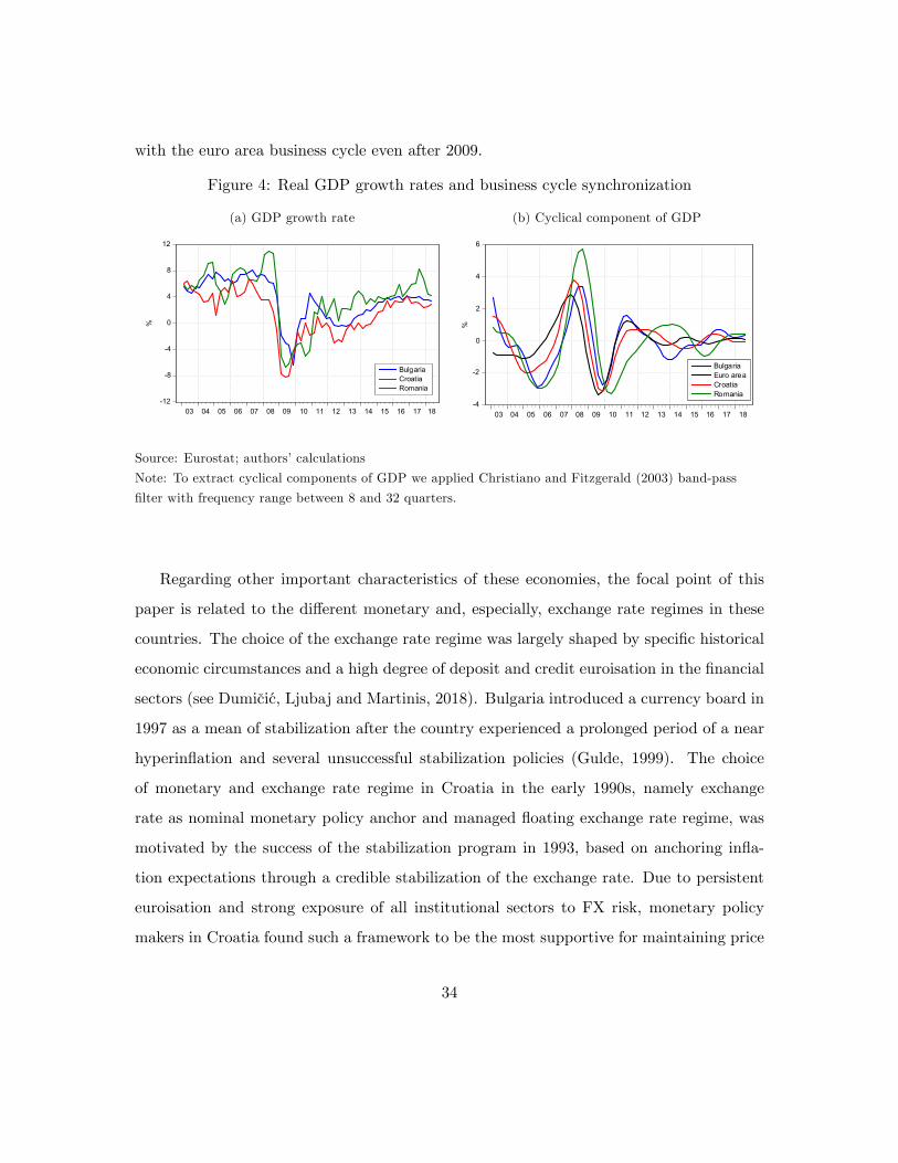
with the euro area business cycle even after 2009.

Figure 4: Real GDP growth rates and business cycle synchronization

(a) GDP growth rate

-12

-8

-4

0

4

8

12

03 04 05 06 07 08 09 10 11 12 13 14 15 16 17 18

BulgariaCroatiaRomania

%

(b) Cyclical component of GDP

-4

-2

0

2

4

6

03 04 05 06 07 08 09 10 11 12 13 14 15 16 17 18

BulgariaEuro areaCroatiaRomania

%Source: Eurostat; authors’calculations

Note: To extract cyclical components of GDP we applied Christiano and Fitzgerald (2003) band-pass

filter with frequency range between 8 and 32 quarters.

Regarding other important characteristics of these economies, the focal point of this

paper is related to the different monetary and, especially, exchange rate regimes in these

countries. The choice of the exchange rate regime was largely shaped by specific historical

economic circumstances and a high degree of deposit and credit euroisation in the financial

sectors (see Dumicic, Ljubaj and Martinis, 2018). Bulgaria introduced a currency board in

1997 as a mean of stabilization after the country experienced a prolonged period of a near

hyperinflation and several unsuccessful stabilization policies (Gulde, 1999). The choice

of monetary and exchange rate regime in Croatia in the early 1990s, namely exchange

rate as nominal monetary policy anchor and managed floating exchange rate regime, was

motivated by the success of the stabilization program in 1993, based on anchoring infla-

tion expectations through a credible stabilization of the exchange rate. Due to persistent

euroisation and strong exposure of all institutional sectors to FX risk, monetary policy

makers in Croatia found such a framework to be the most supportive for maintaining price

34

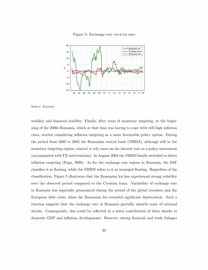
Figure 5: Exchange rate vis-à-vis euro

-15

-10

-5

0

5

10

15

20

04 05 06 07 08 09 10 11 12 13 14 15 16 17 18

Bulgarian levCroatian kunaRomanian leu

%

Source: Eurostat

stability and financial stability. Finally, after years of monetary targeting, at the begin-

ning of the 2000s Romania, which at that time was having to cope with still high inflation

rates, started considering inflation targeting as a more favourable policy option. During

the period from 2003 to 2005 the Romanian central bank (NBRM), although still in the

monetary targeting regime, started to rely more on the interest rate as a policy instrument

(accompanied with FX interventions). In August 2005 the NBRM finally switched to direct

inflation targeting (Popa, 2008). As for the exchange rate regime in Romania, the IMF

classifies it as floating, while the NBRM refers to it as managed floating. Regardless of the

classification, Figure 5 illustrates that the Romanian leu has experienced strong volatility

over the observed period compared to the Croatian kuna. Variability of exchange rate

in Romania was especially pronounced during the period of the global recession and the

European debt crisis, when the Romanian leu recorded significant depreciation. Such a

reaction suggests that the exchange rate in Romania partially absorbs some of external

shocks. Consequently, this could be reflected in a lower contribution of these shocks to

domestic GDP and inflation developments. However, strong financial and trade linkages

35

with the euro area suggest that the contributions of external shocks in Romania could still

be fairly pronounced.

36

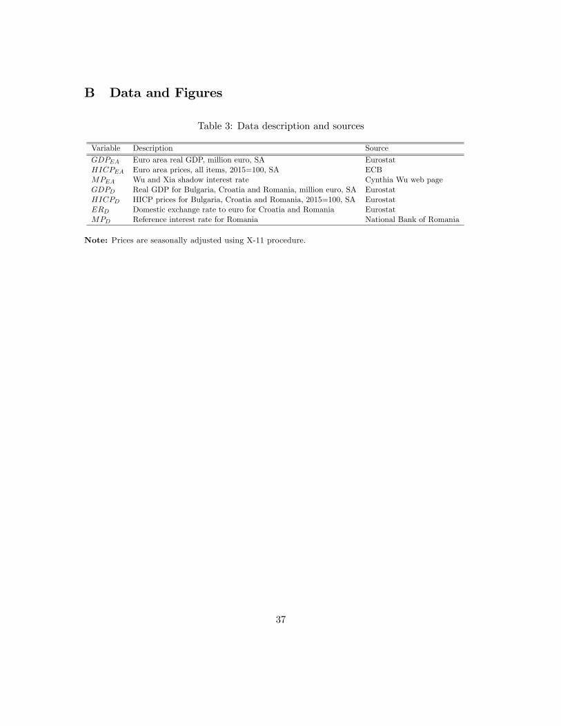
B Data and Figures

Table 3: Data description and sources

Variable Description Source

GDPEA Euro area real GDP, million euro, SA EurostatHICPEA Euro area prices, all items, 2015=100, SA ECBMPEA Wu and Xia shadow interest rate Cynthia Wu web pageGDPD Real GDP for Bulgaria, Croatia and Romania, million euro, SA EurostatHICPD HICP prices for Bulgaria, Croatia and Romania, 2015=100, SA EurostatERD Domestic exchange rate to euro for Croatia and Romania EurostatMPD Reference interest rate for Romania National Bank of Romania

Note: Prices are seasonally adjusted using X-11 procedure.

37

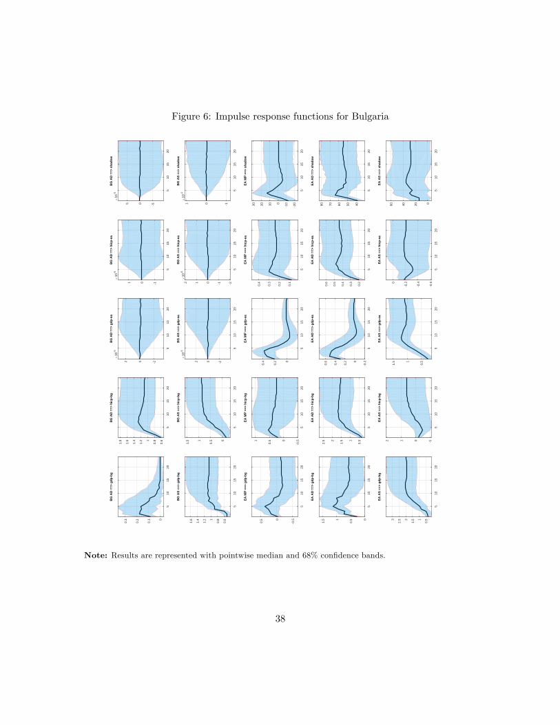
Figure 6: Impulse response functions for Bulgaria

510

1520

0

0.1

0.2

0.3

BG

AD

==>

gd

p-b

g

510

1520

0.6

0.81

1.2

1.4

1.6

1.8

BG

AD

==>

hic

p-b

g

510

1520

-202

10-6

BG

AD

==>

gd

p-e

a

510

1520

-101

10-6

BG

AD

==>

hic

p-e

a

510

1520

-505

10-5

BG

AD

==>

sh

ado

w

510

1520

0.6

0.81

1.2

1.4

1.6

BG

AS

==>

gd

p-b

g

510

1520

0

0.51

1.5

BG

AS

==>

hic

p-b

g

510

1520

-202

10-6

BG

AS

==>

gd

p-e

a

510

1520

-2-101210

-6B

G A

S =

=> h

icp

-ea

510

1520

-10110

-4B

G A

S =

=> s

had

ow

510

1520

-0.50

0.5

EA

MP

==>

gd

p-b

g

510

1520

-0.50

0.51

EA

MP

==>

hic

p-b

g

510

1520

0

0.2

0.4

EA

MP

==>

gd

p-e

a

510

1520

0.1

0.2

0.3

0.4

EA

MP

==>

hic

p-e

a

510

1520

-20

-100102030

EA

MP

==>

sh

ado

w

510

1520

0

0.51

1.5

EA

AD

==>

gd

p-b

g

510

1520

0.51

1.52

2.5

EA

AD

==>

hic

p-b

g

510

1520

-0.20

0.2

0.4

0.6

EA

AD

==>

gd

p-e

a

510

1520

0.2

0.3

0.4

0.5

0.6

EA

AD

==>

hic

p-e

a

510

1520

4050607080

EA

AD

==>

sh

ado

w

510

1520

0.51

1.52

2.53

EA

AS

==>

gd

p-b

g

510

1520

-1012

EA

AS

==>

hic

p-b

g

510

1520

0.51

1.5

EA

AS

==>

gd

p-e

a

510

1520

-0.6

-0.4

-0.20

EA

AS

==>

hic

p-e

a

510

1520

0204060

EA

AS

==>

sh

ado

w

Note: Results are represented with pointwise median and 68% confidence bands.

38

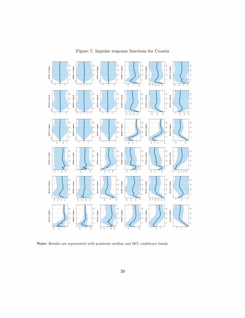
Figure 7: Impulse response functions for Croatia

510

1520

0

0.2

0.4

HR

AD

==>

gd

p-h

r

510

1520

0.1

0.2

0.3

0.4

HR

AD

==>

hic

p-h

r

510

1520

-0.4

-0.20

0.2

HR

AD

==>

eu

rhrk

510

1520

-1

-0.50

0.51

10-6

HR

AD

==>

gd

p-e

a

510

1520

-505

10-7

HR

AD

==>

hic

p-e

a

510

1520

-202

10-5

HR

AD

==>

sh

ado

w

510

1520

-0.20

0.2

HR

ER

==>

gd

p-h

r

510

1520

0.1

0.2

0.3

0.4

HR

ER

==>

hic

p-h

r

510

1520

-0.20

0.2

HR

ER

==>

eu

rhrk

510

1520

-505

10-7

HR

ER

==>

gd

p-e

a

510

1520

-4-2024

10-7

HR

ER

==>

hic

p-e

a

510

1520

-2-1012

10-5

HR

ER

==>

sh

ado

w

510

1520

0.6

0.81

1.2

1.4

HS

AS

==>

gd

p-h

r

510

1520

-0.20

0.2

HS

AS

==>

hic

p-h

r

510

1520

-0.6

-0.4

-0.20

HS

AS

==>

eu

rhrk

510

1520

-202

10-6

HS

AS

==>

gd

p-e

a

510

1520

-101

10-6

HS

AS

==>

hic

p-e

a

510

1520

-505

10-5

HS

AS

==>

sh

ado

w

510

1520

-0.50

0.5

EA

MP

==>

gd

p-h

r

510

1520

0

0.2

0.4

0.6

EA

MP

==>

hic

p-h

r

510

1520

-0.20

0.2

EA

MP

==>

eu

rhrk

510

1520

0

0.2

0.4

EA

MP

==>

gd

p-e

a

510

1520

0.1

0.2

0.3

0.4

EA

MP

==>

hic

p-e

a

510

1520

-20020

EA

MP

==>

sh

ado

w

510

1520

0

0.51

EA

AD

==>

gd

p-h

r

510

1520

0.2

0.4

0.6

0.81

1.2

EA

AD

==>

hic

p-h

r

510

1520

-0.20

0.2

0.4

EA

AD

==>

eu

rhrk

510

1520

-0.20

0.2

0.4

0.6

EA

AD

==>

gd

p-e

a

510

1520

0.2

0.4

0.6

EA

AD

==>

hic

p-e

a

510

1520

4050607080

EA

AD

==>

sh

ado

w

510

1520

123

EA

AS

==>

gd

p-h

r

510

1520

-1

-0.50

EA

AS

==>

hic

p-h

r

510

1520

-0.8

-0.6

-0.4

-0.20

0.2

EA

AS

==>

eu

rhrk

510

1520

0.51

1.5

EA

AS

==>

gd

p-e

a

510

1520

-0.6

-0.4

-0.20

EA

AS

==>

hic

p-e

a

510

1520

0204060

EA

AS

==>

sh

ado

w

Note: Results are represented with pointwise median and 68% confidence bands.

39

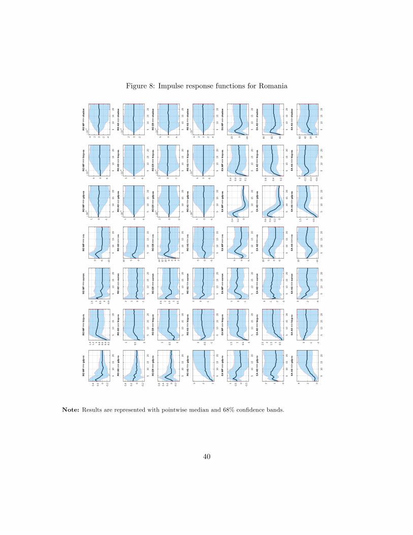
Figure 8: Impulse response functions for Romania

510

1520

-0.20

0.2

0.4

RO

MP

==>

gd

p-r

o

510

1520

0.2

0.4

0.6

0.81

1.2

1.4

RO

MP

==>

hic

p-r

o

510

1520

-0.50

0.51

1.5

RO

MP

==>

eu

rro

n

510

1520

-10-50

RO

MP

==>

i-ro

510

1520

-101

10-5R

O M

P =

=> g

dp

-ea

510

1520

-505

10-6R

O M

P =

=> h

icp

-ea

510

1520

-4-202410

-4RO

MP

==>

sh

ado

w

510

1520

-0.20

0.2

0.4

RO

AD

==>

gd

p-r

o

510

1520

0

0.51

RO

AD

==>

hic

p-r

o

510

1520

-1012

RO

AD

==>

eu

rro

n

510

1520

0510

RO

AD

==>

i-ro

510

1520

-10110

-5RO

AD

==>

gd

p-e

a

510

1520

-505

10-6R

O A

D =

=> h

icp

-ea

510

1520

-202

10-4R

O A

D =

=> s

had

ow

510

1520

-0.20

0.2

0.4

0.6

RO

ER

==>

gd

p-r

o

510

1520

0

0.51

RO

ER

==>

hic

p-r

o

510

1520

0.51

1.52

2.5

RO

ER

==>

eu

rro

n

510

1520

2468101214

RO

ER

==>

i-ro

510

1520

-20210

-5RO

ER

==>

gd

p-e

a

510

1520

-10110

-5RO

ER

==>

hic

p-e

a

510

1520

-505

10-4R

O E

R =

=> s

had

ow

510

1520

123

RO

AS

==>

gd

p-r

o

510

1520

-1

-0.50

RO

AS

==>

hic

p-r

o

510

1520

-101

RO

AS

==>

eu

rro

n

510

1520

-505

RO

AS

==>

i-ro

510

1520

-101

10-5R

O A

S =

=> g

dp

-ea

510

1520

-505

10-6R

O A

S =

=> h

icp

-ea

510

1520

-4-202410

-4RO

AS

==>

sh

ado

w

510

1520

-0.50

0.51

EA

MP

==>

gd

p-r

o

510

1520

0

0.51

1.5

EA

MP

==>

hic

p-r

o

510

1520

-101

EA

MP

==>

eu

rro

n

510

1520

-505

EA

MP

==>

i-ro

510

1520

0

0.2

0.4

EA

MP

==>

gd

p-e

a

510

1520

0.1

0.2

0.3

0.4

EA

MP

==>

hic

p-e

a

510

1520

-20020

EA

MP

==>

sh

ado

w

510

1520

012

EA

AD

==>

gd

p-r

o

510

1520

0.51

1.52

2.5

EA

AD

==>

hic

p-r

o

510

1520

-3-2-10

EA

AD

==>

eu

rro

n

510

1520

-50510

EA

AD

==>

i-ro

510

1520

0

0.2

0.4

0.6

EA

AD

==>

gd

p-e

a

510

1520

0.2

0.4

0.6

EA

AD

==>

hic

p-e

a

510

1520

406080

EA

AD

==>

sh

ado

w

510

1520

024

EA

AS

==>

gd

p-r

o

510

1520

-2-10

EA

AS

==>

hic

p-r

o

510

1520

-4-20

EA

AS

==>

eu

rro

n

510

1520

-10010

EA

AS

==>

i-ro

510

1520

0.51

1.5

EA

AS

==>

gd

p-e

a

510

1520

-0.6

-0.4

-0.20

EA

AS

==>

hic

p-e

a

510

1520

0204060

EA

AS

==>

sh

ado

w

Note: Results are represented with pointwise median and 68% confidence bands.

40

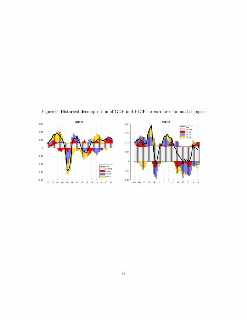
Figure 9: Historical decomposition of GDP and HICP for euro area (annual changes)

05 06 07 08 09 10 11 12 13 14 15 16 17 18-0.08

-0.06

-0.04

-0.02

0

0.02

0.04

0.06gdp-ea

data

baseline

EA MP

EA AD

EA AS

05 06 07 08 09 10 11 12 13 14 15 16 17 18-0.02

-0.01

0

0.01

0.02

0.03

0.04hicp-ea

data

baseline

EA MP

EA AD

EA AS

41

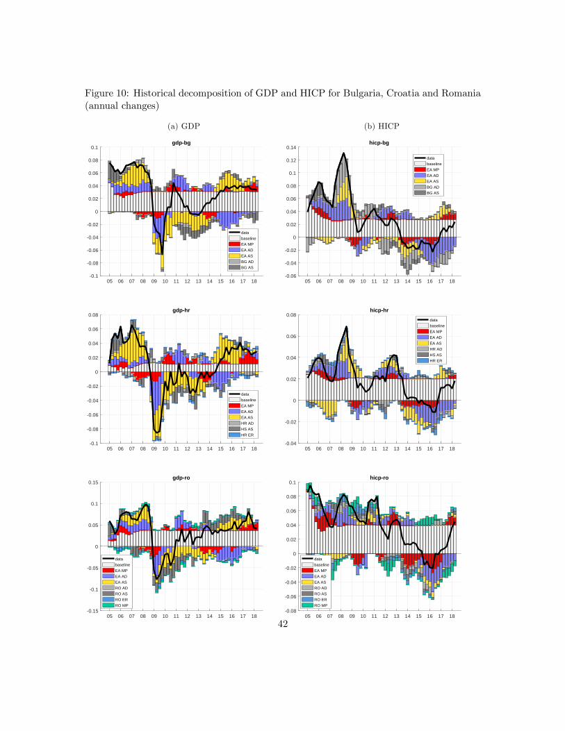
Figure 10: Historical decomposition of GDP and HICP for Bulgaria, Croatia and Romania(annual changes)

(a) GDP

05 06 07 08 09 10 11 12 13 14 15 16 17 18-0.1

-0.08

-0.06

-0.04

-0.02

0

0.02

0.04

0.06

0.08

0.1gdp-bg

data

baseline

EA MP

EA AD

EA AS

BG AD

BG AS

(b) HICP

05 06 07 08 09 10 11 12 13 14 15 16 17 18-0.06

-0.04

-0.02

0

0.02

0.04

0.06

0.08

0.1

0.12

0.14hicp-bg

data

baseline

EA MP

EA AD

EA AS

BG AD

BG AS

05 06 07 08 09 10 11 12 13 14 15 16 17 18-0.1

-0.08

-0.06

-0.04

-0.02

0

0.02

0.04

0.06

0.08gdp-hr

data

baseline

EA MP

EA AD

EA AS

HR AD

HS AS

HR ER

05 06 07 08 09 10 11 12 13 14 15 16 17 18-0.04

-0.02

0

0.02

0.04

0.06

0.08hicp-hr

data

baseline

EA MP

EA AD

EA AS

HR AD

HS AS

HR ER

05 06 07 08 09 10 11 12 13 14 15 16 17 18-0.15

-0.1

-0.05

0

0.05

0.1

0.15gdp-ro

data

baseline

EA MP

EA AD

EA AS

RO AD

RO AS

RO ER

RO MP

05 06 07 08 09 10 11 12 13 14 15 16 17 18-0.08

-0.06

-0.04

-0.02

0

0.02

0.04

0.06

0.08

0.1hicp-ro

data

baseline

EA MP

EA AD

EA AS

RO AD

RO AS

RO ER

RO MP

42

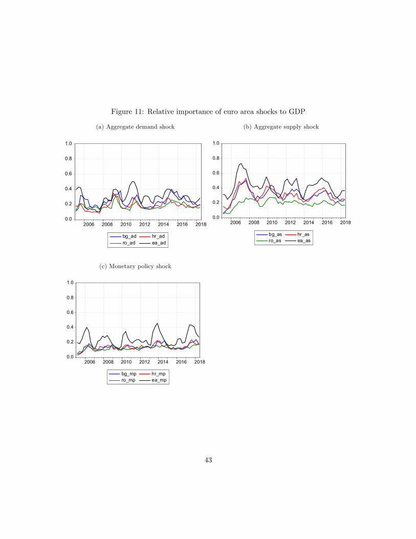
Figure 11: Relative importance of euro area shocks to GDP

(a) Aggregate demand shock

0.0

0.2

0.4

0.6

0.8

1.0

2006 2008 2010 2012 2014 2016 2018

bg_ad hr_adro_ad ea_ad

(b) Aggregate supply shock

0.0

0.2

0.4

0.6

0.8

1.0

2006 2008 2010 2012 2014 2016 2018

bg_as hr_asro_as ea_as

(c) Monetary policy shock

0.0

0.2

0.4

0.6

0.8

1.0

2006 2008 2010 2012 2014 2016 2018

bg_mp hr_mpro_mp ea_mp

43

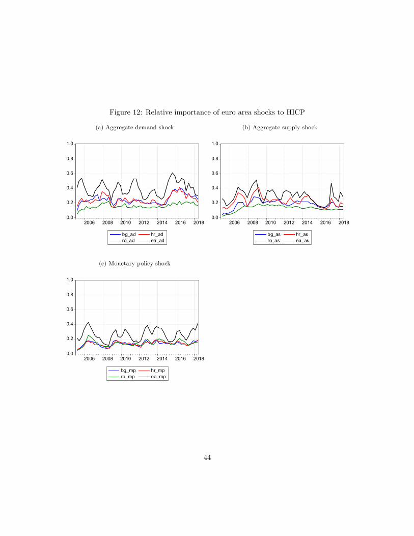
Figure 12: Relative importance of euro area shocks to HICP

(a) Aggregate demand shock

0.0

0.2

0.4

0.6

0.8

1.0

2006 2008 2010 2012 2014 2016 2018

bg_ad hr_adro_ad ea_ad

(b) Aggregate supply shock

0.0

0.2

0.4

0.6

0.8

1.0

2006 2008 2010 2012 2014 2016 2018

bg_as hr_asro_as ea_as

(c) Monetary policy shock

0.0

0.2

0.4

0.6

0.8

1.0

2006 2008 2010 2012 2014 2016 2018

bg_mp hr_mpro_mp ea_mp

44

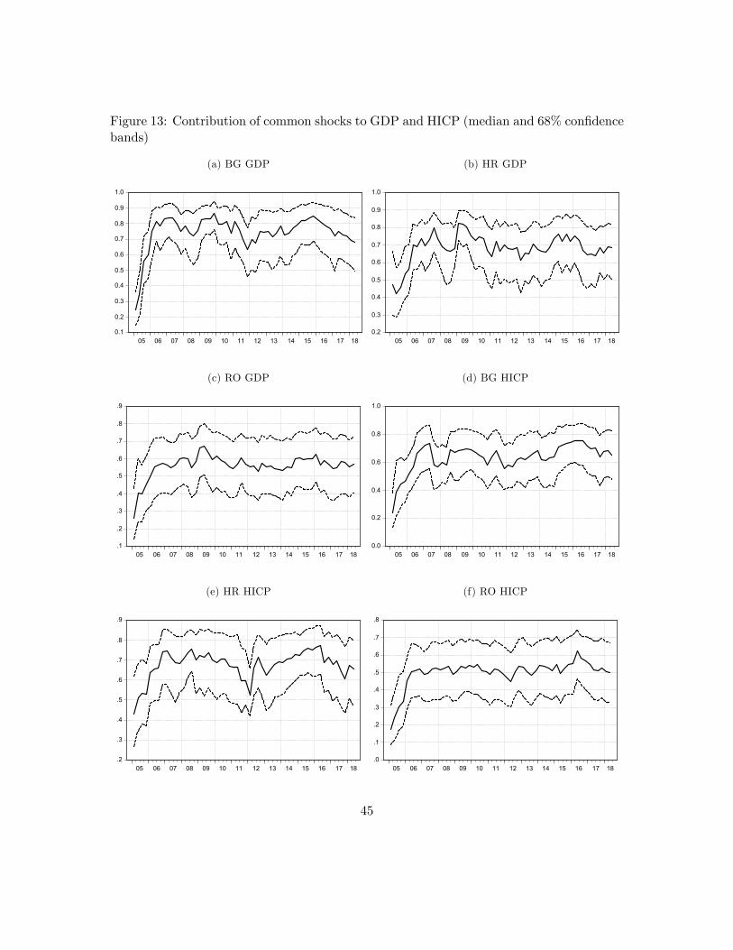
Figure 13: Contribution of common shocks to GDP and HICP (median and 68% confidencebands)

(a) BG GDP

0.1

0.2

0.3

0.4

0.5

0.6

0.7

0.8

0.9

1.0

05 06 07 08 09 10 11 12 13 14 15 16 17 18

(b) HR GDP

0.2

0.3

0.4

0.5

0.6

0.7

0.8

0.9

1.0

05 06 07 08 09 10 11 12 13 14 15 16 17 18

(c) RO GDP

.1

.2

.3

.4

.5

.6

.7

.8

.9

05 06 07 08 09 10 11 12 13 14 15 16 17 18

(d) BG HICP

0.0

0.2

0.4

0.6

0.8

1.0

05 06 07 08 09 10 11 12 13 14 15 16 17 18

(e) HR HICP

.2

.3

.4

.5

.6

.7

.8

.9

05 06 07 08 09 10 11 12 13 14 15 16 17 18

(f) RO HICP

.0

.1

.2

.3

.4

.5

.6

.7

.8

05 06 07 08 09 10 11 12 13 14 15 16 17 18

45

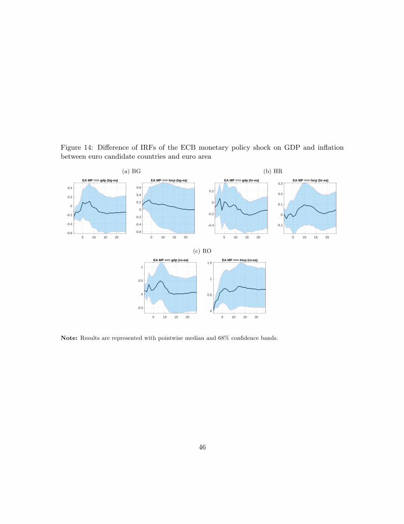
Figure 14: Difference of IRFs of the ECB monetary policy shock on GDP and inflationbetween euro candidate countries and euro area

(a) BG

5 10 15 20-0.6

-0.4

-0.2

0

0.2

0.4

EA MP ==> gdp (bg-ea)

5 10 15 20

-0.6

-0.4

-0.2

0

0.2

0.4

0.6

EA MP ==> hicp (bg-ea)

(b) HR

5 10 15 20

-0.4

-0.2

0

0.2

EA MP ==> gdp (hr-ea)

5 10 15 20

-0.1

0

0.1

0.2

0.3EA MP ==> hicp (hr-ea)

(c) RO

5 10 15 20

-0.5

0

0.5

1

EA MP ==> gdp (ro-ea)

5 10 15 20

0

0.5

1

1.5EA MP ==> hicp (ro-ea)

Note: Results are represented with pointwise median and 68% confidence bands.

46

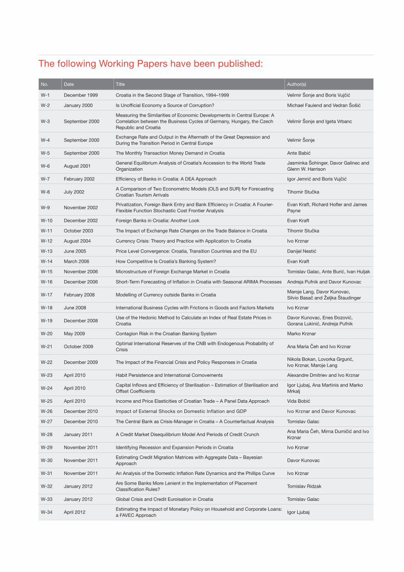
The following Working Papers have been published:

No. Date Title Author(s)

W-1 December 1999 Croatia in the Second Stage of Transition, 1994–1999 Velimir Šonje and Boris Vujčić

W-2 January 2000 Is Unofficial Economy a Source of Corruption? Michael Faulend and Vedran Šošić

W-3 September 2000Measuring the Similarities of Economic Developments in Central Europe: A Correlation between the Business Cycles of Germany, Hungary, the Czech Republic and Croatia

Velimir Šonje and Igeta Vrbanc

W-4 September 2000Exchange Rate and Output in the Aftermath of the Great Depression and During the Transition Period in Central Europe

Velimir Šonje

W-5 September 2000 The Monthly Transaction Money Demand in Croatia Ante Babić

W-6 August 2001General Equilibrium Analysis of Croatia’s Accession to the World Trade Organization

Jasminka Šohinger, Davor Galinec and Glenn W. Harrison

W-7 February 2002 Efficiency of Banks in Croatia: A DEA Approach Igor Jemrić and Boris Vujčić

W-8 July 2002A Comparison of Two Econometric Models (OLS and SUR) for Forecasting Croatian Tourism Arrivals

Tihomir Stučka

W-9 November 2002Privatization, Foreign Bank Entry and Bank Efficiency in Croatia: A Fourier-Flexible Function Stochastic Cost Frontier Analysis

Evan Kraft, Richard Hofler and James Payne

W-10 December 2002 Foreign Banks in Croatia: Another Look Evan Kraft

W-11 October 2003 The Impact of Exchange Rate Changes on the Trade Balance in Croatia Tihomir Stučka

W-12 August 2004 Currency Crisis: Theory and Practice with Application to Croatia Ivo Krznar

W-13 June 2005 Price Level Convergence: Croatia, Transition Countries and the EU Danijel Nestić

W-14 March 2006 How Competitive Is Croatia’s Banking System? Evan Kraft

W-15 November 2006 Microstructure of Foreign Exchange Market in Croatia Tomislav Galac, Ante Burić, Ivan Huljak

W-16 December 2006 Short-Term Forecasting of Inflation in Croatia with Seasonal ARIMA Processes Andreja Pufnik and Davor Kunovac

W-17 February 2008 Modelling of Currency outside Banks in CroatiaMaroje Lang, Davor Kunovac, Silvio Basač and Željka Štaudinger

W-18 June 2008 International Business Cycles with Frictions in Goods and Factors Markets Ivo Krznar

W-19 December 2008Use of the Hedonic Method to Calculate an Index of Real Estate Prices in Croatia

Davor Kunovac, Enes Đozović, Gorana Lukinić, Andreja Pufnik

W-20 May 2009 Contagion Risk in the Croatian Banking System Marko Krznar

W-21 October 2009Optimal International Reserves of the CNB with Endogenous Probability of Crisis

Ana Maria Čeh and Ivo Krznar

W-22 December 2009 The Impact of the Financial Crisis and Policy Responses in CroatiaNikola Bokan, Lovorka Grgurić, Ivo Krznar, Maroje Lang

W-23 April 2010 Habit Persistence and International Comovements Alexandre Dmitriev and Ivo Krznar

W-24 April 2010Capital Inflows and Efficiency of Sterilisation – Estimation of Sterilisation and Offset Coefficients

Igor Ljubaj, Ana Martinis and Marko Mrkalj

W-25 April 2010 Income and Price Elasticities of Croatian Trade – A Panel Data Approach Vida Bobić

W-26 December 2010 Impact of External Shocks on Domestic Inflation and GDP Ivo Krznar and Davor Kunovac

W-27 December 2010 The Central Bank as Crisis-Manager in Croatia – A Counterfactual Analysis Tomislav Galac

W-28 January 2011 A Credit Market Disequilibrium Model And Periods of Credit CrunchAna Maria Čeh, Mirna Dumičić and Ivo Krznar

W-29 November 2011 Identifying Recession and Expansion Periods in Croatia Ivo Krznar

W-30 November 2011Estimating Credit Migration Matrices with Aggregate Data – Bayesian Approach

Davor Kunovac

W-31 November 2011 An Analysis of the Domestic Inflation Rate Dynamics and the Phillips Curve Ivo Krznar

W-32 January 2012Are Some Banks More Lenient in the Implementation of Placement Classification Rules?

Tomislav Ridzak

W-33 January 2012 Global Crisis and Credit Euroisation in Croatia Tomislav Galac

W-34 April 2012Estimating the Impact of Monetary Policy on Household and Corporate Loans: a FAVEC Approach

Igor Ljubaj

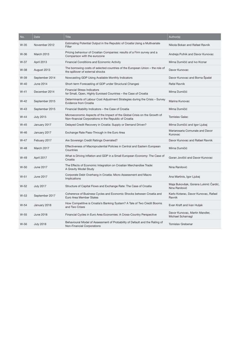
No. Date Title Author(s)

W-35 November 2012 Estimating Potential Output in the Republic of Croatia Using a Multivariate Filter Nikola Bokan and Rafael Ravnik

W-36 March 2013Pricing behaviour of Croatian Companies: results of a Firm survey and a Comparison with the eurozone

Andreja Pufnik and Davor Kunovac

W-37 April 2013 Financial Conditions and Economic Activity Mirna Dumičić and Ivo Krznar

W-38 August 2013The borrowing costs of selected countries of the European Union – the role of the spillover of external shocks

Davor Kunovac

W-39 September 2014 Nowcasting GDP Using Available Monthly Indicators Davor Kunovac and Borna Špalat

W-40 June 2014 Short-term Forecasting of GDP under Structural Changes Rafal Ravnik

W-41 December 2014Financial Stress Indicators for Small, Open, Highly Euroised Countries – the Case of Croatia

Mirna Dumičić

W-42 September 2015Determinants of Labour Cost Adjustment Strategies during the Crisis – Survey Evidence from Croatia

Marina Kunovac

W-43 September 2015 Financial Stability Indicators – the Case of Croatia Mirna Dumičić

W-44 July 2015Microeconomic Aspects of the Impact of the Global Crisis on the Growth of Non-financial Corporations in the Republic of Croatia

Tomislav Galac

W-45 January 2017 Delayed Credit Recovery in Croatia: Supply or Demand Driven? Mirna Dumičić and Igor Ljubaj

W-46 January 2017 Exchange Rate Pass-Through in the Euro AreaMariarosaria Comunale and Davor Kunovac

W-47 Febuary 2017 Are Sovereign Credit Ratings Overrated? Davor Kunovac and Rafael Ravnik

W-48 March 2017Effectiveness of Macroprudential Policies in Central and Eastern European Countries

Mirna Dumičić

W-49 April 2017What is Driving Inflation and GDP in a Small European Economy: The Case of Croatia

Goran Jovičić and Davor Kunovac

W-50 June 2017The Effects of Economic Integration on Croatian Merchandise Trade: A Gravity Model Study

Nina Ranilović

W-51 June 2017Corporate Debt Overhang in Croatia: Micro Assessment and Macro Implications

Ana Martinis, Igor Ljubaj

W-52 July 2017 Structure of Capital Flows and Exchange Rate: The Case of CroatiaMaja Bukovšak, Gorana Lukinić Čardić, Nina Ranilović

W-53 September 2017Coherence of Business Cycles and Economic Shocks between Croatia and Euro Area Member States

Karlo Kotarac, Davor Kunovac, Rafael Ravnik

W-54 January 2018How Competitive is Croatia’s Banking System? A Tale of Two Credit Booms and Two Crises

Evan Kraft and Ivan Huljak

W-55 June 2018 Financial Cycles in Euro Area Economies: A Cross-Country PerspectiveDavor Kunovac, Martin Mandler, Michael Scharnagl

W-56 July 2018Behavioural Model of Assessment of Probability of Default and the Rating of Non-Financial Corporations

Tomislav Grebenar

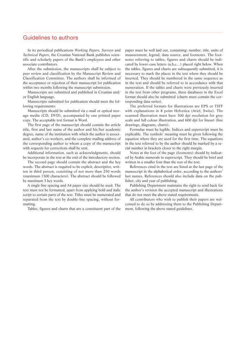
Guidelines to authors

In its periodical publications Working Papers, Surveys and Technical Papers, the Croatian National Bank publishes scien-tific and scholarly papers of the Bank’s employees and other associate contributors.

After the submission, the manuscripts shall be subject to peer review and classification by the Manuscript Review and Classification Committee. The authors shall be informed of the acceptance or rejection of their manuscript for publication within two months following the manuscript submission.

Manuscripts are submitted and published in Croatian and/or English language.

Manuscripts submitted for publication should meet the fol-lowing requirements:

Manuscripts should be submitted via e-mail or optical stor-age media (CD, DVD), accompanied by one printed paper copy. The acceptable text format is Word.

The first page of the manuscript should contain the article title, first and last name of the author and his/her academic degree, name of the institution with which the author is associ-ated, author’s co-workers, and the complete mailing address of the corresponding author to whom a copy of the manuscript with requests for corrections shall be sent.

Additional information, such as acknowledgments, should be incorporate in the text at the end of the introductory section.

The second page should contain the abstract and the key words. The abstract is required to be explicit, descriptive, writ-ten in third person, consisting of not more than 250 words (maximum 1500 characters). The abstract should be followed by maximum 5 key words.

A single line spacing and A4 paper size should be used. The text must not be formatted, apart from applying bold and italic script to certain parts of the text. Titles must be numerated and separated from the text by double-line spacing, without for-matting.

Tables, figures and charts that are a constituent part of the

paper must be well laid out, containing: number, title, units of measurement, legend, data source, and footnotes. The foot-notes referring to tables, figures and charts should be indi-cated by lower-case letters (a,b,c…) placed right below. When the tables, figures and charts are subsequently submitted, it is necessary to mark the places in the text where they should be inserted. They should be numbered in the same sequence as in the text and should be referred to in accordance with that numeration. If the tables and charts were previously inserted in the text from other programs, these databases in the Excel format should also be submitted (charts must contain the cor-responding data series).

The preferred formats for illustrations are EPS or TIFF with explanations in 8 point Helvetica (Ariel, Swiss). The scanned illustration must have 300 dpi resolution for grey scale and full colour illustration, and 600 dpi for lineart (line drawings, diagrams, charts).

Formulae must be legible. Indices and superscript must be explicable. The symbols’ meaning must be given following the equation where they are used for the first time. The equations in the text referred to by the author should be marked by a se-rial number in brackets closer to the right margin.

Notes at the foot of the page (footnotes) should by indicat-ed by Arabic numerals in superscript. They should be brief and written in a smaller font than the rest of the text.

References cited in the text are listed at the last page of the manuscript in the alphabetical order, according to the authors’ last names. References should also include data on the pub-lisher, city and year of publishing.

Publishing Department maintains the right to send back for the author’s revision the accepted manuscript and illustrations that do not meet the above stated requirements.

All contributors who wish to publish their papers are wel-comed to do so by addressing them to the Publishing Depart-ment, following the above stated guidelines.

The Croatian National Bank publications

Croatian National Bank – Annual ReportRegular annual publication surveying annual monetary and general economic developments as well as statistical data.

Croatian National Bank – Semi-annual ReportRegular semi-annual publication surveying semi-annual mon-etary and general economic developments and statistical data.

Banks BulletinPublication providing survey of data on banks.

Croatian National Bank – BulletinRegular monthly publication surveying monthly monetary and general economic developments and monetary statistics.

Croatian National Bank – Working PapersOccasional publication containing shorter scientific papers written by the CNB employees and associate contributors.

Croatian National Bank – SurveysOccasional publication containing scholarly papers written by the CNB employees and associate contributors.

Croatian National Bank – Technical PapersOccasional publication containing papers of informative char-acter written by CNB employees and associate contributors.

The Croatian National Bank also issues other publications such as, for example, numismatic issues, brochures, publica-tions in other media (CD-ROM, DVD), books, monographs and papers of special interest to the CNB as well as proceed-ings of conferences organised or co-organised by the CNB, ed-ucational materials and other similar publications.

ISSN 1334-0131 (online)