Essays in

The theory and measurement of consumer behaviour

Essays in The theory and measurement of consumer behaviour

in honour of Sir Richard Stone Edited by ANGUS DEATON

CAMBRIDGE UNIVERSITY PRESS Cambridge London New York New Rochelle Melbourne Sydney

CAMBRIDGE UNIVERSITY PRESS

Cambridge, New York, Melbourne, Madrid, Cape Town, Singapore, Sao Paulo

Cambridge University Press

The Edinburgh Building, Cambridge CB2 8RU, UK

Published in the United States of America by Cambridge University Press, New York

www.cambridge.org

Information on this title: www.cambridge.org/9780521225656

© Cambridge University Press 1981

This publication is in copyright. Subject to statutory exception

and to the provisions of relevant collective licensing agreements,

no reproduction of any part may take place without the written

permission of Cambridge University Press.

First published 1981

This digitally printed version 2008

A catalogue record for this publication is available from the British Library ISBN 978-0-521-22565-6 hardback

ISBN 978-0-521-06755-3 paperback

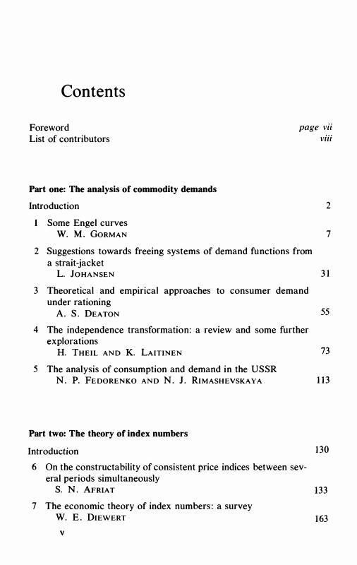
Contents

Foreword List of contributors

Part one: The analysis of commodity demands

page vii viii

Introduction 2

Some Engel curves W. M. GORMAN 7

2 Suggestions towards freeing systems of demand functions from a strait-jacket

L. JOHANSEN 31

3 Theoretical and empirical approaches to consumer demand under rationing

A. S. DEATON 55

4 The independence transformation: a review and some further explorations

H. THEIL AND K. LAITINEN 73

5 The analysis of consumption and demand in the USSR N. P. FEDORENKO AND N. J. RIMASHEVSKAYA 113

Part two: The theory of index numbers

Introduction 130

6 On the constructability of consistent price indices between sev-eral periods simultaneously

S. N . AFRIAT 133

7 The economic theory of index numbers : a survey W. E . DIEWERT 163

v

vi CONTENTS

Part three: The consumptfon function and durable goods

Introduction

8 Testing neoclassical models of the demand for consumer dura­bles

J. MUELLBAUER

9 Liquidity and inflation effects on consumers' expenditure D. F. HENDRY AND T. VON UNGERN-

STERNBERG

Part four: Other aspects: fertility and labour supply

Introduction

10 On labour supply and commodity demands A. B . ATKINSON AND N. H. STERN

1 1 Child spacing and numbers : an empirical analysis M. NERLOVE AND A. RAZIN

Bibliography of Sir Richard Stone's works 1936-79 Index of names Subject index

210

213

237

262

265

297

325 338 341

Foreword

Sir Richard Stone retired from his chair in Cambridge in September 1980. To mark the occasion, this volume has been written in his honour. It is not afestschrift after the usual mould, where friends and colleagues contrib­ute a diverse collection of papers . Sir Richard's achievements have been too broad and his disciples too many to permit a single collection along such lines. Instead, I have taken one single field in which Sir Richard has been preeminent, and attempted to bring together a first-rate collection of papers in that field. Many of the authors are close friends or ex-colleagues of Sir Richard's , but several have had little more than professional con­tact. However, all are indebted to him through his scientific work, and in contributing to this volume are united in their wish to honour him and to acknowledge their indebtedness . In editing the volume it is my hope that the best way of honouring Sir Richard and commemorating his retirement is the preparation of a volume of the best current work in the economics of consumer behaviour. The papers published here are representative of a wide range of contemporary research in the field and only a few important topics are not covered at some point. They provide a good indication not only of the state of the art but also of the extraordinary area over which Sir Richard's own work has been an influence.

A N GUS DEATON

Princeton, October 1979

VII

Contributors

S. N. AFRIAT

A. B . ATKINSON

A. S. DEATON

W. E. DIEWERT

N. P. FEDORENKO

W. M. GORMAN

D. F. HENDRY

L. JOHANSEN

K. LAITINEN

J. MUELLBAUER

M. NERLOVE

A. RAZIN

N. J. RIMASHEVSKA YA

N. H. STERN

H. THEIL

THOMAS VON UNGERN-STERNBERG

viii

University of Ottawa London School of Economics University of Bristol and Princeton University University of British Columbia Central Institute for Mathematical Economics , Moscow London School of Economics and Johns Hopkins University London School of Economics Institute of Economics, University of Oslo University of Chicago Birkbeck College, London Northwestern University University of Tel-Aviv Central Institute for Mathematical Economics, Moscow University of Warwick University of Chicago University of Bonn

PART ONE

The analysis of commodity demands

Introduction to part one

In a volume dedicated to Sir Richard Stone, it is appropriate that first consideration should be given to the theory and measurement of commodity demands . Sir Richard's own great monograph, The Measurement of Consumers' Expenditure and Behaviour in the United Kingdom [5 1]* retains its classic status in applied econometrics to this day . The research programme established there and in the 1954 Economic Journal article [ 48] on the linear expenditure system is still flourishing and the five papers in part one represent several aspects of it .

The first set of topics concern the appropriate choice of functional form for empirical demand equations . In [5 1 ], Sir Richard and his coworkers adopted a largely pragmatic approach using a loglinear constant elasticity form. This has great advantages in computation and allows a much more flexible research strategy than is possible with more complex non-linear equations in which all commodities are dealt with simultaneously . However, as has been known for a long time, loglinear demand functions for all commodities are inconsistent with utility theory in that they cannot permit the predicted demands to add up to the predetermined sum of expenditures. This reflects a quite general problem: how do we choose functional forms which are convenient to work with, which allow the easy incorporation of such information as we possess about the nature of individual demands, and which are consistent with the theory? The first two papers in this section are addressed to that question.

The paper by Terence Gorman investigates a generalization of perhaps the most obvious type of functional form for Engel curves , a polynominal structure with expenditures related to powers of income. Important examples of this are well-known: linear Erigel curves, characterized by the so-called 'Gorman polar form' , (Gorman, 1961) - the class to which the linear expenditure system belongs, as well as the quadratic expenditure system more recently described and estimated in Pollak and Wales ( 1978) and Howe, Pollak and Wales ( 1980). In his paper, Gorman proves a remarkable result : essentially, the quadratic case is as general as we can go. Demand equations with more than three terms in income (e .g.

* References given by numbers in brackets are to Sir Richard's own publications which are contained in a separate bibliography at the end of the book. Other citations are given by author and date, e.g., Gorman (1%1).

2

Introduction 3

a constant, linear and quadratic terms) are degenerate in the sense that the matrix of coefficients linking each demand to each power of income cannot be of rank greater than three. On the other hand, useful functional forms such as

W1 = a1 + f31 log m + y1(log m)2

or

for budget shares w1 and income m, are allowed without restrictions on the coefficients. In recent years , more and more large samples of data on individual households are being analysed at the microeconomic level, so that such flexible Engel curves will be increasingly required while, at the same time, the rank restriction ought to be testable in practice.

An alternative approach to the specification of demands is to assume a particular utility function and to derive demands from it, the linear expenditure system being the classic example. Such an approach has two main drawbacks. First, it is rarely straightforward to derive demand func­tions explicitly and second, it is extremely difficult to choose a utility function which will guarantee some desirable empirical feature in the de­mands. For example, the estimated functions often embody strong prior restrictions on the quantities which are being estimated, often precluding genuine measurement at all; for the case of the linear expenditure system see Deaton ( 1974b; 1975). Both these difficulties have largely been over­come by two recent developments : first, the use of duality methods and, second, the invention and widespread use of what are known as 'flexible functional forms' . Through duality , preferences are described indirectly through the indirect utility function or cost (expenditure) function and these representations are connected very simply, by differentiation or in­tegration, to the commodity demands. (For descriptions of this theory see, for example, Diewert ( 1974; 198 1), McFadden ( 1978), or, at a simpler level, Deaton and Muellbauer ( 1980a, chapters 2 and 3).) The closer rela­tionship between demands and preferences makes it possible to choose preference orderings which are tailored to specific applications. Particu­larly useful are the flexible functional forms which are general enough and contain sufficiently many parameters to guarantee an arbitrarily close local approximation (usually second order) to any general utility function. Such a choice guarantees that the demand functions have enough free parameters to prevent any possibility of prior restrictions between income and price elasticities other than those generally required by utility theory.

A complementary strategy is advocated in the second paper, that by Leif Johansen. He suggests that separability theory be used to break up

4 ANA L Y S I S O F CO M M O D I T Y D E M A ND S

the overall utility function into branches , each of which can be given a dif­ferent functional form tailored to the group of goods being modelled. Within such a scheme, we might have the linear expenditure system for allocating to broad groups , say food, leisure and services, while the sub­utility function for food could be such as to permit quadratic Engel curves for bread, cereals, meat and so forth as functions of total food expendi­ture. Different structures could then be chosen for leisure goods and for services as the circumstances and the data dictate . How all this can be fitted together is the subject of the paper.

The two empirical papers which follow cover two topics in which there have been major developments in recent years . That by Angus Deaton discusses some of the theoretical and practical problems which arise if we wish to estimate demand functions when some of the consumption levels are determined outside the consumer's control. This is the area of ra­tioning theory and here again we have a topic in which much of the seminal work was done in Cambridge by the group around Sir Richard Stone in the early days of the Department of Applied Economics: see par­ticularly the papers by Rothbarth ( 1941) , Tobin and Houthakker ( 195 1 ) and the survey by Tobin ( 1952) which virtually closed the subject for nearly twenty years . Ifwe are to construct tests for the presence ofrationing (for example of whether individuals are voluntarily or involuntarily unem­ployed), it is necessary to be able to compare rationed and unrationed de­mands for the goods which can be freely chosen. Deaton presents a tech­nique for linking constrained and unconstrained cost functions and applies it to a model which is a generalization of the linear expenditure system. On annual British data, housing expenditure is treated as a prede­termined commitment and the results suggest that this may be a more appropriate assumption than its opposite , that such expenditures are always at their optimal levels. At the same time, the treatment through ra­tioning resolves at least some of the apparent conflict between the evi­dence and the homogeneity requirement of utility theory.

The paper by Henri Theil and Kenneth Laitinen surveys a recent devel­opment not tied to but usually associated with empirical and theoretical work using the Rotterdam model. In the earliest days of utility theory, pioneers such as Gossen, Jevons, Edgeworth, Marshall and Pigou typi­cally assumed that wants were ' independent' of one another so that pref­erences could be represented as the sum of specific satisfactions from each good. Such an assumption simplifies the analysis of demand but unfortunately imposes restrictions which are typically rejected by the evi­dence: see, among others , the studies by Barten ( 1969) and Deaton ( 1974a) . What Theil and Laitinen do, however, is to define new goods or commodities as linear combinations of the original goods, with respect to

Introduction 5

which an additive structure of preferences can be maintained. This tech­nique, the ' independence transformation' , is surveyed in the paper together with a number of empirical applications including the demand for meats and the demand for leisure, its complements and substitutes .

The final paper in the section is about demand analysis as a tool of eco­nomic policy and planning. Sir Richard Stone has always seen the ulti­mate aim of his own work as being economic policy-making and succes­sive versions of the linear expenditure system have been incorporated in the Cambridge growth model over the years : see Cambridge, Department of Applied Economics ( 1962-74) and Deaton ( 1975). The paper presented here, by Academicians Fedorenko and Rimashevskaya of the Central In­stitute for Mathematical Economics in Moscow, surveys the techniques used for projecting consumers' demands in Russia in a situation where such projection is of more than academic interest. The approach, as befits policy-making, is an eclectic one but, almost inevitably, the linear expend­iture system has a central role . It must be very rare in economics for one specific model and one specific paper to exert such an ubiquitous influ­ence in both theoretical and policy-related discussions .

References

Barten, A. P. ( 1969), ' Maximum likelihood estimation of a complete system of de­mand equations' , European Economic Review, 1, pp. 7-73.

Cambridge, Department of Applied Economics ( 1%2-74) , A programme for growth, Vols. I -XII, Chapman and Hall, London.

Deaton, A. S. ( 1974a) , 'The analysis of consumer demand in the United Kingdom 1900- 1970' , Econometrica, 42, pp. 341 -67.

( 1974b), 'A reconsideration of the empirical implications of additive prefer­ences' , Economic Journal, 84, pp. 338-48.

( 1975), Models and projections of demand in post-war Britain, Chapman and Hall, London.

Deaton, A. S. and J. Muellbauer ( 1980) , Economics and consumer behavior, Cam­bridge University Press, New York.

Diewert, W. E. ( 1974), 'Applications of duality theory' , Chapter 3 in Intriligator, M. D. and D. A. Kendrick (eds . ) , Frontiers of quantitative economics, Vol. II, North-Holland, Amsterdam.

( 1981 ), 'Duality approaches to microeconomic theory' , in Arrow, K. J. and M. Intriligator (eds. ) , Handbook of Mathematical Economics, North-Holland, Amsterdam.

Gorman, W. M. ( 1961 ) , ' On a class of preference fields' , Metroeconomica, 13, pp. 53-6.

Howe, H., R. A. Pollak, and T. J. Wales ( 1980), 'Theory and time series estima­tion of the quadratic expenditure system' , Econometrica, 48, pp. 123 1 -47.

McFadden, D. ( 1978), 'Cost, revenue and profit functions' , in Fuss, M. and D. McFadden (eds . ) , Production economics: a dual approach to theory and ap­plications, North-Holland, Amsterdam.

6 AN A L Y S I S O F CO M M O D I T Y D E M A N D S

Pollak, R. A . and T . J . Wales ( 1978), 'Estimation of complete demand systems from household budget data' , American Economic Review, 68, pp. 348-59.

Rothbarth, E. ( 1941 ) , 'The measurement of change in real income under condi­tions of rationing' , Review of Economic Studies, 8, pp. 100-7.

Tobin, J . ( 1952), 'A survey of the theory of rationing' , Econometrica, 20, pp. 5 1 2-53 .

Tobin, J. and H. S. Houthakker (1951 ) , 'The effects of rationing on demand elas­ticities' , Review of Economic Studies, 18, pp. 140-53.

1 Some Engel curves1

W. M . G O R M A N

0 Introduction

In this paper I investigate the conditions under which rational2 individuals have Engel curves of the type

x1 = L bri(p)•V(m) for each good i ( 1 ) rER

in the usual notation, where R is a finite set. They are of interest for three, related, uses:

(i) for fitting to surveys ; (ii) as a generalisation of linear Engel curves, which have turned out to

be useful in several contexts , particularly as the solution of the ag­gregation problem

x1 = Ji(p, </>(m)) for each i, m = (m. , m2, • • . , mr) (2)

where m, is the income of the tth household, xi , the market demand for good i, and </>(.) a scalar aggregate ;

(iii) as the solution of the more general version of (2) in which </>(. ) is a vector of aggregates.

Incidentally , the l/J(.) may contain equivalent adult and other correc­tions .

On the other hand, they are rendered less interesting by the fact that m in ( 1 ) , and each m, in (2), stands for money income.

If the Engel curves in ( 1 ) represent well-behaved preferences, we find that

(i) The rank R(B(p)) of the coefficient matrix B(p) = [bri(p)] is at most 3 .

(ii) When R(B(p)) = 3,3 either (a) each .pr(m) = m(log mY, and each r E R is an integer, or (b) each .pr(m) = mr+i , or (c) each .pr(m) = m sin(r log m) or m cos(r log m), for each r � 0,4 with 0 E R in each case. In section 4 I conjecture that R = {-mw, -(m - l)w, .. ., 0, w, . . . , nw} with a few gaps sometimes .

(iii) When R(B(p)) = 3 the cost function underlying ( 1 ) may be written

m = </>(o:(p) , {3(p), y(p), u) (3)

7

8 w. M . GO R M A N

where a( . ) , {3( . ) , y(.) are unit cost functions, which may be thought of as corresponding to baskets of commodities. It is tempting to rewrite (3) in primal form as

u = f(x) = max{F(a(y), b(z), c(w))IY + z + w s x} (4)

where a(. ) , b( .) , c( .) are the corresponding conica/5 production func­tions, in which case <f>(. , u) in (3) would be the cost function corre­sponding to u = F(.) . Unfortunately </>(. , u), though conical, is not necessarily concave, so that this interpretation is not strictly justi­fied. When it is, we may say that the various goods affect our welfare through the basic wants a, b, c - an interpretation which remains en­lightening even when not strictly justified.

(iv) (iib) clearly includes the polynomials. When R(B(p)) = 3, then </>(. , u ) in (3) is additively homogeneous, as well as conical - that is, mul­tiplicatively homogeneous . That is,

so that

<f>(>..li, u) = >..<f>(li, u); <f>(li + µ,e, u) = <f>(li, u) + µ, (5)

<f>(>..8 + µ,e, u) = >..<f>(li, u) + µ,

<f>(a, {3, y, u) = a + (/3 - a)l/J((y - a)/({3 - a), u)6 say (6)

where e = ( 1 , 1 , . . . , 1 ) , >.. :2: 0, so that, where justified, (4) may be rewritten

u = f(x) = max{.F(a(y), b(z))ic(x - y - z) :2: l} say (7)

so that c = 1 may be thought of as the satisfaction of a basic 'need', or, if you like, an overhead of existence.

These results are extended to a wider class of Engel curves at the end of section 3 .

(v) Since R(B) s 3 , quadratics are particularly interesting. The cost function is then

m = a(p) + 8(p)/(1 - ue(p))

where

8 = {3 - a, e = (y - {3)/(/3 - a) (vi) When R(B(p)) = 2, the cost function may be written

m = <f>(a(p), {3(p), u)

(8)

(9)

( 10)

where a( . ) , {3( .) are once more unit cost functions and <f>(. , u) is con­ical but not necessarily either concave or additively homogeneous .

Some Engel curves 9

Iff it is closed concave, the corresponding primal may be written

u = f(x) = max{F(a(y) , b(z))IY + z s; x} ( 1 1)

where u = F(.) is the dual of </>(. , u), a(.), b( .) of a(.), {3(. ) . When </>( . , u) i s additively homogeneous, ( 10) may be written

m = a(p) + u8(p), 8 = f3 - a ( 12)

so that the Engel curves are straight lines, as in the standard case re­ferred to in the opening paragraph.

(vii) When R(B(p)) = 1 , u = f(x) is homothetic , and the Engel curves straight lines radiating from the origin.

1 Preliminaries

It will be convenient to write the equations of the Engel curves in terms of the budget shares WJ = PJXJ/m, and accordingly to use the logarithmic cost function

h(q, u) =log g(p, u) = log m; qJ = log PJ, for each j ( 1 )

since

WJ = hJ(q, u), for each j (2)

where I use suffixes to function names to denote differentiation. Consider complete systems of Engel curves of the type

hJ(q, u) = L a(r, j; q)<f>(r; h(q, u)); for each good j (3) rER

where R is a finite set. This is a curious notation. One would expect the labels r ,j to appear as

subscripts , as in arJ(q) , or superscripts as in arJ(q), rather tlian as argu­ments , as in a(r, j; q). However, I will be using subscripts to denote deriv­atives, and powers will come into the analysis so often that I cannot use the superscript notation either. To distinguish between the discrete labels such as r ,j and the continuous variables such as q, m, I will put the labels before, and the variables after, the ';' in each case . It will frequently be convenient not to mention the latter explicitly, writing a(r, j) for a(r, j; q), for instance.

Assume without loss of generality that this representation is unique so that

I O w. M . GO R M A N

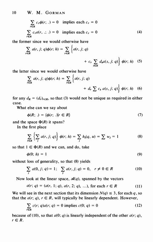
L cr<f>(r; . ) = 0 implies each Cr = 0 rER

L Cra(r, . ; . ) = 0 implies each Cr = 0 rER

the former since we would otherwise have

L a(r, j; q)<f>(r; h) = L { a(r, j; q) rER rER

(4)

+ Cr L d8a(s, j; q)} <f>(r; h) (5) SER

the latter since we would otherwise have

L a(r, j; q)<f>(r; h) = L { a(r, j; q) �R �R

+ dr L Cs a(s , j; q)} <f>(r; h) (6)

for any dn = (dr)ren. so that (3) would not be unique as required in either case.

What else can we say about

<f>(R; .) = {<f>(r; . )Ir E R}

and the space <l>(R) it spans? In the first place

(7)

L {'L a(r, j; q)} <f>(r; h) = L h;(q, u) = L w; = 1 (8) rER j j

so that 1 E <l>(R) and we can, and do, take

<f>(O; h) = 1

without loss of generality, so that (8) yields

L a(O, j ; q) = 1 ; L a(r, j; q) = 0, r '/: 0 E R j j

Now look at the linear space, d(q), spanned by the vectors

(9)

( 10)

a(r; q) = (a(r, 1 ; q), a(r, 2 ; q), . . . ), for each r E R ( 1 1 ) We will see in the next section that its dimension N(q) s 3 , for each q , so that the a(r; q) , r E R, will typically be linearly dependent. However,

L c(r; q)a(r; q) = 0 implies c(O; q) = 0 ( 12) rER

because of ( 10) , so that a(O; q) is linearly independent of the other a(r; q) , r E R.

Some Engel curves 11

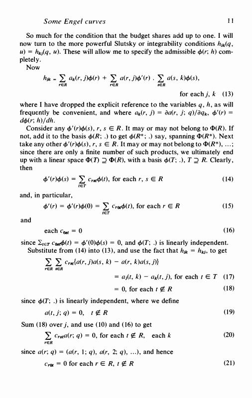
So much for the condition that the budget shares add up to one. I will now turn to the more powerful Slutsky or integrability conditions hJk(q, u) = hk/q, u). These will allow me to specify the admissible <f>(r; h) com­pletely.

Now

hJk = L ak(r, j)<f>(r) + L a(r, j)<f>'(r) . L a(s , k)<f>(s), rER rER sER

for each j, k ( 13) where I have dropped the explicit reference to the variables q, h , as will frequently be convenient, and where ak(r, j) = aa(r, j; q)/aqk, <f>'(r) = d<f>(r; h)/ dh.

Consider any <f>'(r)<f>(s) , r, s E R . It may or may not belong to <l>(R). If not, add it to the basis <f>(R; .) to get <f>(R* ; .) say, spanning <l>(R*). Next take any other <f>'(r)<f>(s) , r, s E R. It may or may not belong to <l>(R*), . . . ; since there are only a finite number of such products, we ultimately end up with a linear space <1>(1) d <l>(R), with a basis <f>(T; . ) , T d R. Clearly, then

<f>'(r)<f>(s) = L Crat<f>(t), for each r, s E R ( 14) IET

and, in particular,

<f>'(r) = <f>'(r)<f>(O) = L Cr0t<f>(t), for each r E R (15) tET

and

each Coat = 0 ( 16)

since �ter c08t<f>(t) = <f>'(O)<f>(s) = 0, and <f>(T; .) is linearly independent. Substitute from ( 14) into ( 13) , and use the fact that hJk = hk;, to get

L L Crat{a(r, j)a(s , k) - a(r, k)a(s, j)} rER sER

= a;(t, k) - ak(t, j), for each t E T ( 17)

= 0, for each t � R

since <f>(T; .) is linearly independent, where we define

a(t, j; q) = O, t � R

Sum ( 1 8) over j, and use ( 10) and ( 16) to get

L Cro1a(r; q) = 0, for each t � R, each k rER

since a(r; q) = (a(r, 1 ; q), a(r, 2; q), . . . ) , and hence

croi = 0 for each r E R, t � R

( 18)

( 19)

(20)

(21 )

1 2 w. M . GO R M A N

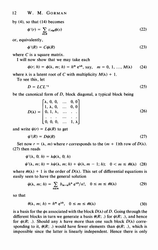
by (4), so that ( 14) becomes

cf>'(r) = L cr0scf>(s) sER

or, equivalently ,

cf>'(R) = Ccf>(R)

where C is a square matrix . I will now show that we may take each

(22)

(23)

cf>(r; h) = cf>(>.. , m ; h) = hm e>..h , say, m = 0, I , . . . , M(>..) (24)

where >.. is a latent root of C with multiplicity M(>..) + I . To see this , let

D = LCL-1

be the canonical form of D, block diagonal, a typical block being [>.. , 0, 0, . . . 0, 01 I , >.. , 0, . . . 0, 0

D(>..) = �· �· �· ::: : : 0, 0, 0, . . . I , >..

and write l/J(r) = Lcf>(R) to get

l/l'(R) = Dl/l(R)

(25)

(26)

(27)

Set now r = (>.. , m) where r corresponds to the (m + l )th row of D(>..) . (27) then reads

I/I'(>.. , O; h) = 11.1/J(A., O; h)

l/J'(>.. , m ; h) = >...µ(>.., m; h) + l/J(A., m - I ; h); 0 < m :::;; m(>..) (28)

where m(>..) + 1 is the order of D(>..) . This set of differential equations is easily seen to have the general solution

so that

.µ(>.., m ; h) = L bm-nhn e .. h/n ! , o :::;; m:::;; m(>..) n�m

fJ(>.. , m ; h) = hm eM, 0 :::;; m :::;; m(>..)

(29)

(30)

is a basis for the .ps associated with the block D(>..) of D. Going through the different blocks in turn we generate a basis fJ(R; .) for l/J(R; .) , and hence for cf>(R; .) . Should any >.. have more than one such block D(>..) corre­sponding to it, fJ(R; .) would have fewer elements than cf>(R; .) , which is impossible since the latter is linearly independent. Hence there is only

Some Engel curves 1 3

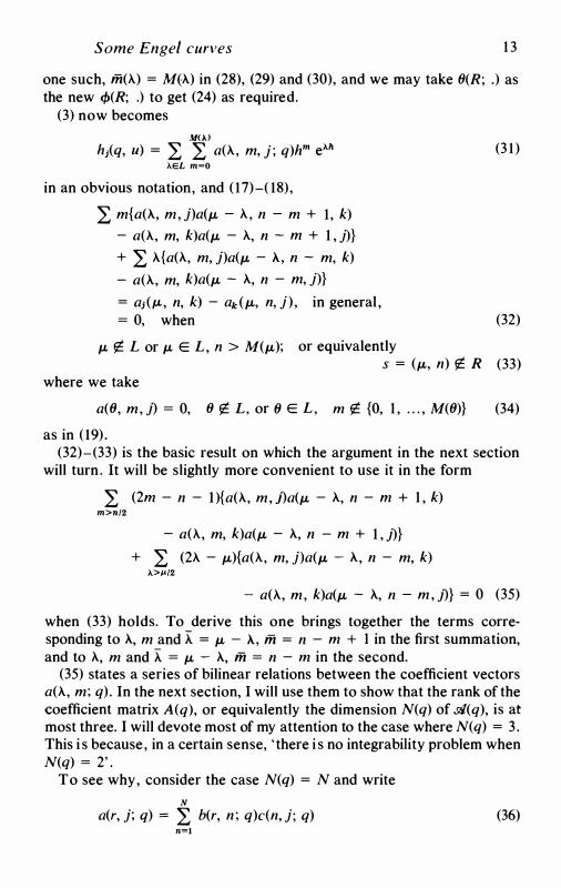
one such, m(A.) = M(A.) in (28), (29) and (30), and we may take 8(R; .) as the new cf>(R; .) to get (24) as required.

(3) now becomes MO.J

hj(q, u) = L L a(A., m, j ; q)hm e>..h >..EL m=O

in an obvious notation, and ( 17)-( 18),

L m{a(A., m, j)a(µ, - A, n - m + 1, k) - a(A., m, k)a(µ, - A, n - m + l , j)} + L A.{a(A, m, j)a(µ, - A, n - m, k) - a(A., m, k)a(µ, - A, n - m, j)} = a1(JL, n, k) - adµ,, n, j) , in general , = 0, when

µ, � L or µ, E L, n > M(µ,); or equivalently

(3 1 )

(32)

s = (µ,, n) � R (33) where we take

a(8, m, J) = 0, 8 � L, or 8 E L, m � {O, I , . . . , M(8)} (34)

as in ( 19) . (32)-(33) is the basic result on which the argument in the next section

will turn. It will be slightly more convenient to use it in the form

L (2m - n - l ){a(A., m, 1)a(µ, - A, n - m + I , k) m>n/2

- a(A., m, k)a(µ, - A, n - m + l , j)} + L (2A. - µ,){a(A., m, j)a(µ, - A, n - m, k)

>..>µ/2

- a(A., m, k)a(µ, - A, n - m , J)} = 0 (35)

when (33) holds. To derive this one brings together the terms corre­sponding to A, m and X = µ, - A, m = n - m + I in the first summation, and to A, m and X = µ, - A, m = n - min the second.

(35) states a series of bilinear relations between the coefficient vectors a(A., m; q) . In the next section, I will use them to show that the rank of the <:oefficient matrix A(q), or equivalently the dimension N(q) of .stl(q), is at most three. I will devote most of my attention to the case where N(q) = 3 . This i s because, in a certain sense, ' there i s no integrability problem when N(q) = 2'.

To see why, consider the case N(q) = N and write N

a(r, j; q) = L b(r, n; q)c(n, j; q) (36) n=I

14 w. M. GO R M A N

to get

h1(q, u) = f { L b(r, n ; q)cJ>(r; h(q, u))} c(n , j; q) (37) n=l rER

Define the gradient of h( . , u) by

h '(q, u) = (h1(q, u), h2(q, u), . . . ) (38)

and choose u1 < u2 < . . . < uN such that h '(q, u1), h' (q, u2), . . . h ' (q, uN) span d(q). Define

O(n; q) = h(q, Un), c(n ; q) = (c(n, 1; q), c(n, 2; q), . . . ) , n = 1 , 2, . . . , N (39)

The Os are functionally independent and

O'(m ; q) = �1 {£ b(r, n ; q)cJ>(r; O(m; q))} c(n; q),

n = 1, 2, . . . , N (40)

Solving this for the c(n; q) in terms of the O'(m; q) and substituting into (37), we get

hJ(q, u) = �1 {£ d(r, n ; q)cJ>(r; h(q, u))} 6J(n , q),

say, for each j (41 ) so that

h(q, u) = H(6( 1 , q) , 6(2, q) , . . . , O(N, q) , u) (42)

given the necessary smoothness and connectivity. Now 6(n, q) = h(q, un) is a logarithmic cost function, each n, and may

without loss of generality be taken to be the logarithmic unit cost function for a fictitious intermediate good, or composite commodity, produced under constant returns - that is, they may be taken to be the logarithmic prices of those intermediate goods. Now there is no integrability problem when there are only two goods, and it is the integrability conditions which I will be examining in section 2. Hence my concentration on the case where N > 2.

So far I have not used the fact that the consumer' s behaviour, and hence the budget shares, is unaffected when prices and income all change in the same proportion. It is easiest to approach this matter indirectly .

Take any 'logarithmic price index' a(q) such that

:L aiq) = 1 (43) j

Some Engel curves 1 5

so that exp a(q) is homogeneous of degree one in the prices p1 = exp qJ. and write

k(q, u) = h(q, u) - a(q) (44)

which may be thought of as a 'real' logarithmic expenditure function. Clearly

:L kJ(q, u) = o (45) j

Now substitute h = k + a into (3 1) to get

M(il.)

k; = L L b(A., m, j)km eA.k (46) A.EL m=O

where

b(A., n , j) = ell.a �� (:) am-n a(A., m, j) unless n = A. = 0 (47)

M(O)

b(O, 0, j) = L ama(O, m , j) - a; (48)

n=O

or, equivalently ,7

a(A., n , j) = e-11.0: �� (:) ( -a)m-n b(A., m, j) unless n = A. = 0 (49)

M(O)

a(O, 0, j) = L (-ar b(O, m, j) + a; (50) m=o

Multiplying each price P; and income m by (J is the same as adding J.L = log (J to each q, h and a. Doing this in (46) and equating coefficients of kn eAk we get

where

b(A., n , j; q + µe) = b(A., n, j; q) , for each A., n , j, q, J.L (5 1)

e = ( 1 , 1 , . . . , I ) (52)

which is clearly sufficient as well as necessary for homogeneity. That the as should be generated by bs, satisfying (5 1)-(52), as in (49)-(50), is therefore both necessary and sufficient for the homogeneity of the Engel system (3 1 ) .

Finally a little more notation. Since the A.s are the latent roots of a gen­eral square matrix C, they may be complex. If so, they come in conjugate pairs . Write

16 W. M . GO R M A N

A. = <r + iT = (<r, T), r = (A., m ) = (<r + iT, m) = (<r, T, m) (53)

R = {(A., m)IA. EL, m = 0, 1 , . . . , M(A.)} (54)

S = {<rl<r + iT E L, some T}, T = {Tl<r + iT E L, some <r} (55)

Note by the way that

0 E R, and hence 0 E L, 0 E S, 0 E T (56)

because C00t = 0, for each t, since <f>'(O; h) = 0 and <f>(T; .) is linearly inde­pendent . It would be surprising were this not so !

2 The main theorem

Theorem l(a ) : If the complete Engel system ( 1 .3) reflects well-behaved preferences, the rank N(q) of its coefficient matrix is at most 3 .

Theorem l(b): When N(q) = 3 , ( 1 .3) takes one of the forms

M

h1(q, u) = a(j; q) + b(j; q)h + c(j; q) L C(m; q)hm ( 1 ) m=l

<T<O

hJ(q, u) = a(j; q) + b(j; q) L B(<r; q) e"h <TES

CT>O

+ c(j; q) L C(<r; q)e"h (2) <TES

r>O

h;(q, u) = a(j; q) + b(j; q) L B(T; q) cos Th TET

r>O

+ c(j; q) L C(T; q) sin Th (3) TET

Proof- Equation ( l .35) will be used repeatedly , so I will record it here:

L (2m - n - l){a(A., m , j)a(µ - A., n - m + 1 , k) m>n/2

- a(A., m, k)a(µ - A., n - m + 1 , J)}

+ L (2A. - µ){a(A., m, j)a(µ - A., n - m, k) A.>µ,/2

- a(A., m, k)a(µ - A., n - m, j)} = 0 (4)

when

µ � L or µ E L, m > M(µ)

I will proceed in a series of lemmas. Lemma I: Suppose S contains a positive element. Then

(5)

Some Engel curves 1 7

a(r, j) = C(r)cU), say, when u � 0 , unless u = r = m = 0 ( 6)

Proof Set

u* = max{u E S} > 0, r* = max{rl(u*, r) E L} � 0 (7)

>..* = u* + iT*, M(>..*) = m*, r* = (>..*, m*)

and define the lexicographic ordering

(8)

r > r' if u > u', or u = u', T > r', or u = u', T = r', m > m' (9)

Set

c(j) = a(r* , J), for each j

and erect the inductive hypothesis

a(r, j) = C(r)c(J), say, for eachj

when

r>F>O

( 10)

( 1 1)

( 12)

I will show that this implies that ( 1 1 ) holds for f too. Since it certainly holds for r*, it will hold for each r > 0.

Take then r* > f > 0 (i) lf X = >..* , m < m*, write down (4) withµ, = 2>..* � L, n = m + m*

- 1, to get

(m* - m){c(j)a(X, m, k) - c(k)a(X, m, j)} = o ( 13)

all the other terms vanishing by the inductive hypothesis ( 1 1 )-( 12) . Hence ( 1 1) holds for r = f = (A_, m) too.

(ii) If X -I >.. * write down (4) withµ, = >.. * + X, n = m* + m, to get

(>..* - X){c(j)a(X, m, k) - c(k)a(X, m, j)} = o ( 14)

so that ( 1 1 ) holds for r = f = (A., m) too. This leaves us with the cases where a- = 0, f < 0. For them we merely

replace the ordering (9) by one in which we put T first at the second stage when u = 0.

This completes the proof of Lemma 1 . Remark: when f = 0, r* + f E R so that (5) does not hold. Lemma 2: If S has a negative element

a(r, j) = B(r)b(j), say, when u::;; 0, unless r = 0 (15)

Corollary: If S "I {O} and

N(q) � 3 ( 16)

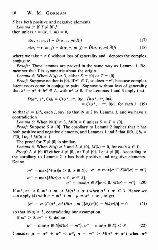
1 8 w. M . GO R M A N

S has both positive and negative elements. Lemma 3: If TI {0},8

then unless r = (<T, T, m) = 0,

a(<T, T, m, j) = D(<T, T, m)d(j)

a(<T, - T, m, j) = ii(<T, T, m, j) = D(<T, T, m) d(j)

( 17)

( 18)

where we take T 2= 0 without loss of generality and -:- denotes the complex conjugate.

Proofs : These lemmas are proved in the same way as Lemma 1 . Re­member that T is symmetric about the origin.

Lemma 4: When N(q) 2= 3, either S = {O} or T = {O}. Proof: Suppose neither is {O}. If T* E T, so does - T* , because complex

latent roots come in conjugate pairs . Suppose without loss of generality that >.. * = <T* + i'T* E L, with <T* 2= 0. The Lemmas 1 and 3 imply that

D(<T* , T* , 0)d1 = C(<T*, T* , O)c1; D(<T*, T*, O)d1 = C(<T*, - T* , O)c1' for each j ( 19)

so that d1 = Ed1, eachj, say, so that N:::::: 2 by Lemma 3, and we have a contradiction.

Lemma 5: When N(q) 2= 3, M(O) = 0 unless S = T = {O}. Proof: Suppose SI {O}. The corollary to Lemma 2 implies that it has

both positive and negative elements, and Lemmas 1 and 2 that B(O, l)b1 = C(O, l )c1 if M(O) > 1 .

The proof for T I {O} i s similar. Lemma 6: When N(q) 2= 3 and L I {O}, M(A.) = 0, for each >.. E L. Proof" L I {O} iff either SI {O}, or TI {O}. Let S I {O} . According to

the corollary to Lemma 2 it has both positive and negative elements . Define

m+ = max{M(<T)l<T > 0, <T E S}, <T+ = max{<T E SIM(<T) = m+}

m- = max{M(<T)l<T < 0, <T E S}, <T- = max{<T E Sl<T < 0, M(<T) = m-} (20)

If m+, m- > 0, m+ + m- > M(<T+ + <T-) when <T+ + <T- E S . Hence we can apply (4) with n = m+ + m-, µ, = <T+ + <T-, to get

(<T+ - <T-)C(<T+, m+)B(<T-, m-){b(j)c(k) - b(k)c(j)} = 0 (2 1)

so that N(q) < 3 , contradicting our assumption. If m+ > 0, m- = 0, define

<T± = min{<T E SIM(<T) = m+}; <T= = min{<T E S} < 09 (22)

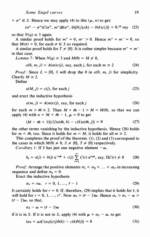
Some Engel curves 1 9

+ a-= E S. Hence we may apply (4) to this (µ, n ) to get:

(a-± - a-=)C(a-±, m+)B(a-=, O){bU)c(k) - b(k)cU)} = 0, 10 say (23)

so that N(q) ::; 3 again. A similar proof holds for m+ = 0, m- > 0. Hence m+ = m- = 0, so

that M(a-) = 0, for each a- E S as required. A similar proof holds for T "I {O}. It is rather simpler because m+ = m­

in that case. Lemma 7: When N(q) 2= 3 and M(O) = M "I 0,

a(O, m, j) = A(m)c(j), say, each j, for each m 2= 2 (24)

Proof: Since L = {O}, I will drop the 0 in a(O, m, j) for simplicity. Clearly M 2= 2.

Define

a(M, J) = c(j) , for each j

and erect the inductive hypothesis

a(m, j) = A(m)c(j) , say, for eachj

(25)

(26)

for each m > m 2= 2. Then M + m - 1 > M = M(O), so that we can apply (4) with n = M + m - 1 , µ, = 0 to get

(M - m + l ){c(J)a(m, k) - c(k)a(m, j)} = O (27)

the other terms vanishing by the inductive hypothesis. Hence (26) holds form = m, too. Since it holds form = M, it holds for all m 2= 2.

This completes the proof of the theorem. ( 1 ) , (2) and (3) correspond to the cases in which M(O) "I 0, S "I {O}, T "I {O} respectively .

Corollary 1 : If S has just one negative element - cu, r•

hJ = a(j) + b(J) e-wh + c(j) L C(r) erw\ say, IIC(r) "I 0 (28) r=t

Proof: Arrange the positive elements a-1 < a-2 < ... < <Tr• in increasing sequence and define a-0 = 0.

Erect the inductive hypothesis

<rr = rcu, r = 0, 1 , ... , f - 1 (29)

It certainly holds for r = 0. If, therefore, (29) implies that it holds for t, it will hold for r = 0, 1 , . . . , r* . Now <rr > (t - l )cu. Hence <rr > <rr - cu > (f - 2)cu, so that,

a-,. - cu = (f - l )cu

if it is in S. If it is not in S, apply (4) withµ, = <rr - cu, to get

(a-,. + cu)C(a-,.){c(j)b(k) - c(k)b(J)} = 0

(30)

(31)

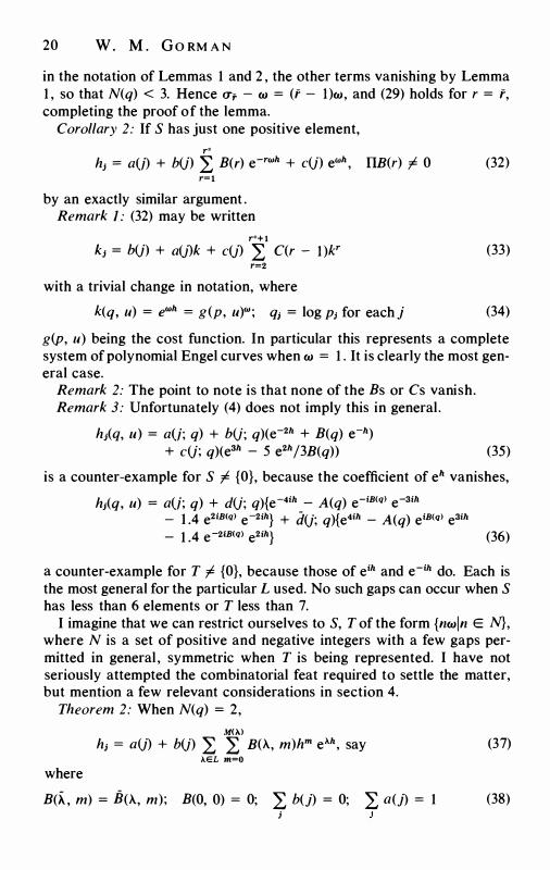
20 w. M. Go RM A N

in the notation of Lemmas 1 and 2 , the other terms vanishing by Lemma 1 , so that N(q) < 3. Hence a-,. - w = (t - l)w, and (29) holds for r = t, completing the proof of the lemma.

Corollary 2: If S has just one positive element, r*

h1 = a(j) + b(j) L B(r) e-rwh + c(j) ewh , IIB(r) I- 0 (32) r=l

by an exactly similar argument . Remark I: (32) may be written

r*+t k1 = b(j) + a(j)k + c(j) L C(r - l)kr (33)

r=2 with a trivial change in notation, where

k(q, u) = ewh = g(p, u)w; q; = log P; for eachj (34)

g(p, u) being the cost function. In particular this represents a complete system of polynomial Engel curves when w = 1 . It is clearly the most gen­eral case.

Remark 2: The point to note is that none of the Bs or Cs vanish. Remark 3: Unfortunately (4) does not imply this in general.

h;(q, u) = a(j; q) + b(j; q)(e-2h + B(q) e-h) + c(j; q)(e3h - 5 e2h/3B(q)) (35)

is a counter-example for S I- {O}, because the coefficient of eh vanishes,

hJ(q , u) = a(j; q) + d(j; q){e-4ih _ A(q) e-iB<q> e-aih _ i.4 e2iB<q> e-2ih} + d(j; q){e4ih _ A(q) eiB<q> eaih _ 1 .4 e-21B<q> e2ih} (36)

a counter-example for T I- {O}, because those of eih and e-ih do. Each is the most general for the particular L used. No such gaps can occur when S has less than 6 elements or T less than 7.

I imagine that we can restrict ourselves to S, T of the form {nwln EN}, where N is a set of positive and negative integers with a few gaps per­mitted in general , symmetric when T is being represented. I have not seriously attempted the combinatorial feat required to settle the matter, but mention a few relevant considerations in section 4.

Theorem 2: When N(q) = 2,

MO.> h; = a(j) + b(j) L L B(A., m)hm e>..h, say (37)

A.EL m=O where

B(i.. , m) = B(A., m); B(O, 0) = O; L b(j) = O; L a(j) = 1 (38) j

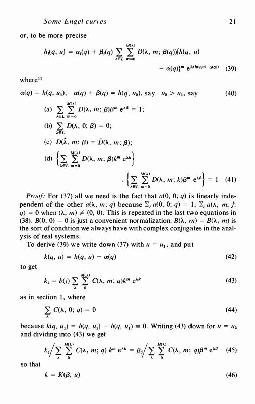
Some Engel curves 2 1

or, to be more precise MO,)

hJ(q, u) = aJ(q) + f31(q) L L D(>.. , m; f3(q)){h(q, u) I.EL m=O

- a(q)}m eA<h(q,u)-<t(q)) (39) where11

a(q) = h(q, u1) ; a(q) + f3(q) = h(q, u2) , say u2 > ui. say (40) M(I.)

(a) L L D(>.. , m ; {3)f3m e>-fJ = 1 ; I.EL m=O

(b) L D(>.. , O; {3) = O; >.EL

(c) D(i.. , m ; {3) = D (>.., m; {3); { M(>.) } (d) L L D(>.. , m; f3)km e>.k I.EL m=O

·

{ L �> D(>.. , m; k)f3m e>.fJ} = 1 (4 1) >.EL m=O

Proof: For (37) all we need is the fact that a(O, O; q) is linearly inde­pendent of the other a(>.., m ; q) because L1 a(O, O; q) = 1 , L1 a(>.., m, j; q) = 0 when (>.. , m) I- (0, 0) . This is repeated in the last two equations in (38). B(O, 0) = 0 is just a convenient normalization. B(i.., m) = B (>.. , m) is the sort of condition we always have with complex conjugates in the anal­ysis of real systems.

To derive (39) we write down (37) with u = u1, and put

to get

k(q, u) = h(q, u) - a(q)

M(>.) k1 = b(j) L L C(>.. , m ; q)km e>-k

>. O

as in section 1 , where

L C(>.. , O; q) = 0 A

(42)

(43)

(44)

because k(q, u1) = h(q, u1) - h(q, u1) = 0. Writing (43) down for u = u2 and dividing into (43) we get

so that I

M(},.) I

M(>.) k; L L C(>.. , m; q) km e>.k = {31 L L C(>.. , m; q)f3m e>-fJ (45)

>. 0 >. 0

k = K(f3, u) (46)

22 w . M. GO R M A N

with

iJk/iJ{3 = L D(A., m; {3)km e>..k = tjJ(k, (3), say >..,m

(47)

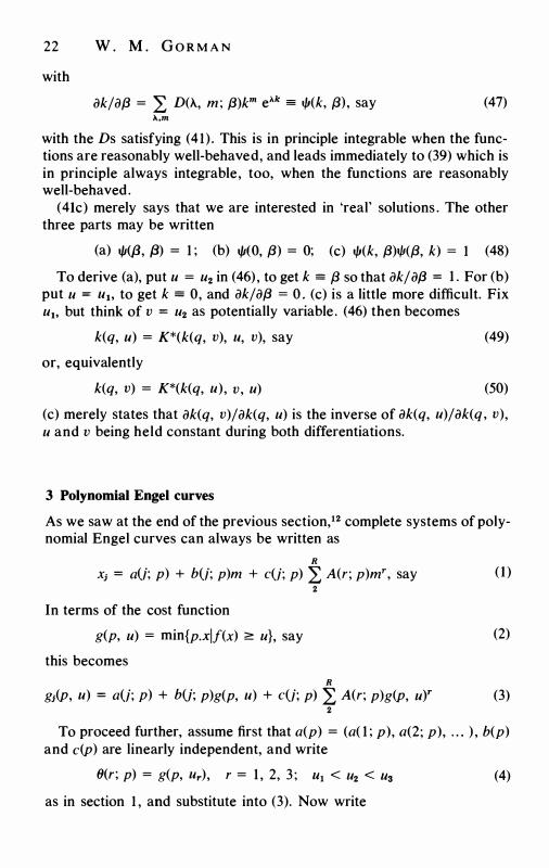
with the Ds satisfying (4 1) . This is in principle integrable when the func­tions are reasonably well-behaved, and leads immediately to (39) which is in principle always integrable, too, when the functions are reasonably well-behaved.

(4lc) merely says that we are interested in 'real' solutions . The other three parts may be written

(a) t/J({3, {3) = l ; (b) t/J(O, {3) = O; (c) tjJ(k, {3)1/1({3, k) = 1 (48)

To derive (a), put u = u2 in (46) , to get k = f3 so that iJk/ iJ{3 = I . For (b) put u = ui. to get k = 0, and iJk/iJ{3 = 0. (c) is a little more difficult. Fix ui. but think of v = u2 as potentially variable . (46) then becomes

k(q, u) = K*(k(q, v), u, v), say

or, equivalently

k(q, v) = K*(k(q, u), v, u)

(49)

(50)

(c) merely states that iJk(q, v)/iJk(q, u) is the inverse of iJk(q, u)/iJk(q, v), u and v being held constant during both differentiations.

3 Polynomial Engel curves

As we saw at the end of the previous section, 12 complete systems of poly­nomial Engel curves can always be written as

R

x; = a(j; p) + b(j; p)m + c(j; p) L A(r; p)mr, say 2

In terms of the cost function

g(p, u) = min{p.xlf(x) ::::: u}, say

this becomes R

( 1 )

(2)

g1(p, u) = a(j; p) + b(j; p)g(p, u) + c(j; p) L A(r; p)g(p, uY (3) 2

To proceed further, assume first that a(p) = (a( l ; p), a(2; p), . . . ) , b(p) and c(p) are linearly independent, and write

8(r; p) = g(p, Ur), r = l , 2, 3 ; U1 < u2 < U3 (4)

as in section 1 , and substitute into (3). Now write

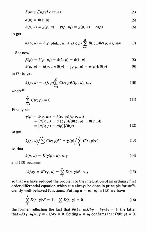
Some Engel curves

a(p) = 8( 1 ; p)

h(p, u) = g(p, u) - g(p, u1) = g(p, u) - a(p)

to get

R

23

(5)

(6)

hJ(p, u) = b(j; p)h(p , u) + c(j; p) L B(r; p)hr(p, u), say (7) r=l

Set now

{3(p) = h(p, U2) = 8(2 ; p) - 8(1 ; p)

k(p, u) = h(p, u)/{3(p) = [g(p, u) - a(p)]//3(p)

in (7) to get R

kJ(p, u) = c(j; p)L C(r; p)kr(p; u), say r=l

where13 R

L C(r; p) = 0 r=l

Finally set

to get

so that

y(p) = k(p, U3) = h(p, Ua)/h(p, U2) = (8(3 ; p) - 8( 1 ; p))/(8(2 ; p) - 8(1 ; p)) = [8(3 ; p) - a(p)]/{3(p)

k(p, u) = K(y(p), u), say

and ( 1 3) becomes R

iJk/iJy = K'(y, u) = L D(r; y)kr, say

(8)

(9)

( 10)

( 1 1)

( 12)

( 13)

( 14)

( 15)

so that we have reduced the problem to the integration of an ordinary first order differential equation which can always be done in principle for suffi­ciently well-behaved functions. Putting u = u3; u2 in ( 15) we have

R

L D(r; y)yr = 1 ; L D(r, y) = 0 ( 16)

the former reflecting the fact that iJK(y, u3)/ay = iJy/iJy = 1 , the latter that iJK(y, u2)/ay = iJl/iJy = 0. Setting u = u1 confirms that D(O; y) = 0.

24 w. M. GO R M A N

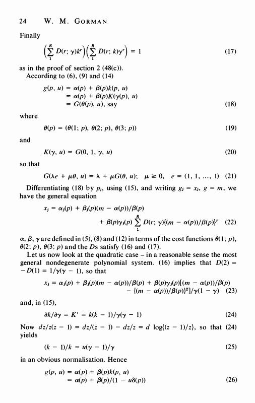
Finally

(± D(r; y)kr) (± D(r; k)yr) = 1 1 1

as in the proof of section 2 (48(c)). According to (6) , (9) and ( 14)

where

and

so that

g(p, u) = a(p) + f3(p)k(p, u) = a(p) + f3(p)K(y(p), u) = G(8(p), u), say

8(p) = (8(1 ; p), 8(2 ; p) , 8(3 ; p))

K(y, u) = G(O, 1 , y, u)

( 17)

( 18)

( 19)

(20)

G(A.e + µ,8, u) = A. + µ,G(8, u) ; µ, � 0, e = ( 1 , 1 , . . . , 1) (21 )

Differentiating ( 1 8) by P;. using ( 15), and writing g1 = x1, g = m, we have the general equation

x1 = a1(p) + f31(p)(m - a(p))/f3(p) R

+ f3(p)y1(p) L D(r; y){(m - a(p))/f3(p}Y (22)

a, {3, y are defined in (5), (8) and ( 12) in terms of the cost functions 8( 1 ; p), 8(2 ; p), 8(3 ; p) and the Ds satisfy ( 16) and ( 17).

Let us now look at the quadratic case - in a reasonable sense the most general nondegenerate polynomial system. ( 16) implies that D(2) = - D( l) = 1/y(y - 1), so that

x1 = a1(p) + f31(p)(m - a(p))/f3(p) + f3(p)y1(p)[(m - a(p))//3(p) - {(m - a(p))/f3(p)}2]/y( l - y) (23)

and, in ( 15),

iJk/iJy = K' = k(k - 1)/y(y - 1) (24)

Now dz/z(z - 1) = dz/(z - 1) - dz/z = d log{(z - 1)/z}, so that (24) yields

(k - 1)/k = u(y - 1)/y (25)

in an obvious normalisation. Hence

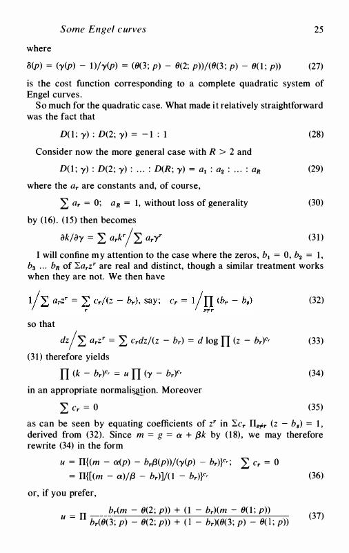
g(p, u) = a(p) + f3(p)k(p, u) = a(p) + f3(p)/( 1 - u8(p)) (26)

Some Engel curves 25

where

8(p) = (y(p) - 1 )/y(p) = (6(3 ; p) - 6(2; p))/(6(3 ; p) - 6( 1 ; p)) (27)

is the cost function corresponding to a complete quadratic system of Engel curves .

So much for the quadratic case. What made it relatively straightforward was the fact that

D( l ; y) : D(2; y) = - 1 : 1 (28)

Consider now the more general case with R > 2 and

D(l ; y) : D(2; y) : . . . : D(R; y) = 01 : o2 : . . . : 08 (29)

where the Or are constants and, of course,

L Or = O; 08 = 1, without loss of generality

by ( 16) . ( 15) then becomes

(30)

iJk/iJy = L Orkr/L OrYr (3 1 )

I will confine my attention to the case where the zeros, b1 = 0, b2 = 1 , b3 . . . b8 of 'Lorzr are real and distinct, though a similar treatment works when they are not. We then have

so that

(32)

dz/ L OrZr = L Crdz/(z - br) = d log IT (z - br)Cr (33) (3 1 ) therefore yields

IT (k - br)Cr = U IT (y - br)Cr (34)

in an appropriate normalisj!.!_ion. Moreover

L Cr = 0 (35)

as can be seen by equating coefficients of zr in 'Lcr Il8,or (z - b,) = 1 , derived from (32). Since m = g = a + f3k by ( 1 8), we may therefore rewrite (34) in the form

U = Il{(m - a(p) - brf3(p))/(y(p) - brW' ; L Cr = 0 = Il{[(m - a)//3 - br)]/0 - brW' (36)

or, if you prefer,

u = n br(m - 6(2 ; p)) + ( 1 - br)(m - 6( 1 ; p)) (37) br(6(3; p) - 6(2; p)) + ( 1 - br)(6(3; p) - 6( 1 ; p))

26 w . M. GO R M A N

Drop (29) and turn to thefully degenerate case in which

>..(p)a(j; p) + µ(p)b(j; p) + v(p)c(j; p) = 0 (38)

where it is not true that >..(p) = µ(p) = y(p) = 0. Since 2.p;:x; = m, µ(p) = 0. Hence either

c(j; p) = 0

yielding the familiar linear Engel system with

g(p, u) = a(p) + {3(p)u

in the obvious normalisation, or

so that

a(j; p) = p(p)c(j; p) , say

X; = b(j; p)m + c(j; p) L A(r; p)mr, say ryf1

(39)

(40)

(41)

(42)

A simplified version of the ,proof leading up to (22) yields ( 15)-(17), (22) , with

a(p) = 8(1 ; p) = 0 (43)

The polynomial Engel curves were generated by putting w = 1 in sec­tion 2(32) . According to section 2(32) a similar analysis applies for gw in the general case discussed there . We can analyse it exactly as we have just done the polynomial case. The results are so similar that I will not spell them out here .

Replacing g( . ) by h( .) in the discussion one can apply the same analysis to section 2( 1) . Note that the polynomial form is guaranteed here , not a further assumption.

4 Concluding remarks

In order to keep this article to a reasonable length, the following remarks have been kept to a perhaps undesirable brevity . The discussion in sec­tions 2 and 3 was entirely local, asking, if you like, when is

X1 = L a(r, i; p)cf>(r; m) ( 1 ) rER to the second order nearer p, m? If so, it will clearly still be so near >..p, >..m, and I will normalise to take m = 1 for simplicity . The main condition was then that the rank N(p) of A(p) = [a(r, i; p)] is :::; 3 .

Let us now assume that representations similar to ( 1 ) are possible throughout an open set !l in p space. Then N(p) :::; 3 throughout !l. Sup-

Some Engel curves 27

pose that N(p) = 3 , some p E 11. Then it will be so throughout a maximal neighbourhood 11(p) � 11 of p. There may be many such disjoint neigh­bourhoods. They will commonly be divided by ii - 1 dimensional sur­faces on which N(p) = 2, and these by ii - 2 dimensional surfaces when N(p) = 1 , when ii is the number of goods. Clearly one cannot move in just any direction and stay in one of these surfaces , as my calculus arguments require. I do not believe that this is a genuine problem, at least if there are sufficient goods, but have not verified this. If you like, apply the arguments for N(p) = 1 , 2, only in cases where this region is solid. N(p) = 3 is, of course, the important case. A similar argument may be applied when max {N(p) IP E 11} = 2, for instance. There the neighbourhoods 11(p) are those in which N(p) = 2, rather than 3 .

Look again at the main theorem as stated at the beginning of section 2. If N = 3 , it states , we are in one of the cases (i), (ii), (iii). Of these, (iii) differs from (ii) only in having purely imaginary exponents , rather than purely real, while (i) is the usual logarithmic limiting case of an expression like (ii). We may therefore concentrate on (ii) as a representative case. It may be written

h;(q, u) = a(j; q) + b(j; q) L B(b ; q)e-bh + c(j; q) L C(c; q)ech (2) bEB cEC

where B = {b > 0 : -b E S}, C = {c > 0 : c E S}. This equation may be treated like (3 . 1) . We set u = ui. u2, u3 in turn, 6(r; q) = h(q, ur) to get

h(q, u) = H(6(1 ) , 6(2), 6(3), u) = 6( 1 ) + il(6(2) - 6( 1) , 6(3) - 6( 1) , u) = a + H(/3, e, u), say (3)

when the second representation is possible because the coefficient of a(i) is 1 .

The bother about this is that ii(. , . , u) has two arguments , and so that there is an integrability problem. One can say a good deal about the nature of a complete solution, but not find it explicitly as one can in the cases dis­cussed in section 3 .

B and C have each at least one element. What made a complete solution possible in section 3 was the assumption that one or other had just one. Let it be B and set B = {w}. Then

n h;(q, u) = a(j; q) + b(j; q)e-wh + C(j; q) L c(r, q) erwh (4)

m=l

Because the coefficients of a(j; q) and b(j; q) both depend only on h , it is possible to reduce the 3 variables in (3) to 1 , not just 2. Because they are 1 , ewh this takes the form

h(q, u) = a + f3K(y, u), y = e//3 (5)

28 w . M. GO R M A N

since K( ., u) has only one argument, there is no integrability condition to be solved.

B = { l} is the polynomial case , B = C = { 1} the quadratic, given w = 1 .

Turn now to the purely imaginary case (iii). B = {w} then corresponds to T = { - w, 0, w} so that we get a direct analogue of the quadratic of the form.

h1 = a(j) + b(j) cos wh + c(j) sin wh (6)

When B = {w}, C = {w, 2w, . . . , nw} say so that S = { - w, 0, w, 2w, nw}. It is not true that S = {-mw, -m - lw, . . . , 0, w, . . . , nw} in gen­eral - section 2(35) and section 2(36) are counter-examples . However, it can14 be shown that this will be so in a 'generic' sense in what I think is a reasonable use of the word; and I suspect that S is always of this form, wherever N = 3, if we allow a few gaps .

Notes

I had planned a contribution worthier of Sir Richard Stone , in which the results would have been related to more general ideas . Unfortunately, I miscalculated the time available and this paper is the rather incomplete result.

The ideas in this paper were first presented to the Quantitative Economics Workshop at the London School of Economics in January 1977 and January 1978. I am grateful to John Wise, who, for the special case of polynomial Engel curves, suggested the probable importance of the rank of the coefficient ma­trix. I am also grateful to John Muellbauer and my colleagues at the LSE for their comments. I thank the SSRC for its funding and the LSE for my col­leagues.

2 Having smooth strictly quasi-concave preferences, and being greedy . 3 Of course the rank of B(p) depends on p in general . It is :s 3 everywhere . If it

equals 3 at a point, it will in an open neighbourhood of it . The analysis of R(B(p)) = 3 , which takes up most of the paper, may be thought of as carried out in such a neighbourhood. Presumably regions in which it takes lower val­ues commonly divide those in which it takes higher. See section 4.

4 Both terms will normally occur. 5 That is, positively homogeneous of degree one. The term is Sydney Afriat' s . 6 l/J(o, u ) = <f>(O, 1 , o, u). 7 Since h = k + a is equivalent to k = h - a , one merely replaces a in

(47)-(48) by - a to get (49)-(50). 8 One can obviously apply the same arguments to T as S, remembering only that

the final results have to be real, in particular T symmetric . 9 S has both positive and negative elements by the corollary to Lemma 2.

IO We sum over (<T, m), (<T' , m') E S such that <T + <T1 = µ, = <T± + <T� , m + m ' = n = m+. When <T<T1 � 0 the term vanishes. When <T<T1 < 0, take <T >

Some Engel curves 29

0, u' < 0. Then 0 � m' � m- = 0. Hence m ' = 0, m = m+ . Hence (u± , m+), (u= , 0) are the only such pair in S.

1 1 Put u = ui, u2 in (39), and eliminate a(j), b(j) from it and the resulting equa­tions.

12 Put w = 1 in section 2(34). 13 To derive ( l l ) : set u = u2 to get k(p, u2) = l , and O = ol/iJPJ = c(j; p) Lr C(r;

p) . Remember that c(p) = (c( l ; p), c(2; p) , . . . ) I- 0 since N = 3 . 14 Added in proof: Consider this as a conjecture . I have lost m y notes o n the point,

and do not even remember the meaning I gave to generic , let alone the proof.

2 Suggestions towards freeing systems of demand functions from a strait-jacket

L E I F J O H A N S E N 1

1 Introduction

The development of complete systems of demand functions has been one of the most important trends in research on consumer demand in the last couple of decades. Richard Stone's Linear Expenditure System and the theoretical approach which he used in establishing this system have been instrumental in this development. The LES system has been widely used both in its original form and in forms modified and generalized in various directions . Several other systems have also appeared. There is no doubt that great advances have been achieved. It seems to me, however, that re­search in this field has, voluntarily , put on a strait-jacket. I have in mind the requirement that all demand functions constituting the system shall be 'of the same form' , differing only in the values of the parameters . The pur­pose of the present paper is to suggest approaches which may help to free theory and applied work from this strait-jacket.

The idea that it would be sound and useful to abandon the requirement that all functions in the system should be of the same form is not entirely uncontroversial. L. J. Lau has argued that such uniformity 'is desirable because it allows all commodities to be treated symmetrically ' . This kind of symmetry does of course possess a sort of aesthetic value, and it is also convenient from a mathematical and computational point of view. Fur­thermore, one might feel that an element of arbitrariness is introduced if the researcher decides to treat different commodities in formally different ways. Nevertheless, although these arguments are attractive, I do not find them compelling.

Now, if one has some ideas about different behaviour of different com­modities in the demand system, then one could of course try to estab­lish a system which is sufficiently general so as to encompass all the forms which one feels are relevant, thus avoiding an a priori association of par­ticular commodities with particular forms. This approach, however, would easily involve too many parameters .

3 1

32 L. J O H A N S E N

It is now quite common to combine information from different sources in establishing systems of demand functions. In particular, it is quite common to establish some properties of the Engel functions (demand as a function of income or total expenditure) on the basis of cross-section in­formation, and next estimate coefficients representing the effects of prices by means of time-series data. In cross-section studies of consumer de­mand where the intention is not to proceed to the construction of com­plete systems including prices, there is more freedom to choose functional forms, and then forms have often been used successfully which are not compatible with any of the well known complete systems which include prices . Among functional forms which have been used successfully for Engel functions, without involving too many parameters, are the Torn­qvist functions . (See particularly H. Wold, 1952, pp. 3-4, 107 -8 and 271 -7. See also P. R. Fisk, 1958-59.) By using different functional forms they are able to describe the behaviour of 'necessities' , ' relative luxu­ries' , and 'luxuries' , and by variations of parameter values also inferior commodities . An example of the use of these functions is given by J. G. van Beeck and H. den Hartog ( 1964) for the Netherlands . (It has also been reported that the functions have been found useful for some groups of commodities in the USSR, see A. Keck, 1968, p. 176.) Another type of Engel curves which has been used successfully is the lognormal probabil­ity function as proposed by J. Aitchison and J. A. C . Brown ( 1954). In this case the same functional form is able to cover qualitatively different cases because of the inflection of the curve and the possibility to use different parts of it for the relevant range by stretching and compressing it.

For systems of Engel curves where the functional form is different as between groups of commodities, two different approaches are conceiv­able at the empirical stage. ( 1 ) One may try the different functional forms for each commodity and choose the one which fits best according to some statistical criterion. (2) One may choose the functional form for each com­modity on a priori grounds . In the latter case the 'a priori' reasons may not necessarily be of a purely intuitive or introspective type. 'Objective needs' might be measured for certain commodities, and the results used as a basis for choosing among the functional forms and for specification of values of certain parameters, for instance saturation levels . Such an ob­jective needs approach is used to some extent in connection with long­term projections and planning in the USSR. See for instance K. K. Val­tukh ( 1975), who argues that the usual demand theory is rather empty unless one introduces some sort of objective information about needs . Such an approach, using investigations of objective needs, ought not to be absolutely alien to neoclassical theory. It was K. Wicksell who wrote: 'Perhaps some day the physiologists will succeed in isolating and eval-

Systems of demand functions 33

uating the various human needs for bodily warmth, nourishment, variety, recreation, stimulation, ornament, harmony etc . , and thereby lay a really rational foundation for the theory of consumption. ' (The quotation is taken from A. E. Andersson ( 1977), who discusses the implications of this view in specific contexts .)

It might be tempting to start out from such rather satisfactory Engel curve systems and construct complete systems of demand functions on this basis. However, this is not easy. In the first place , the Tornqvist func­tions and the Aitchison-Brown type of functions do not satisfy the adding-up condition, except for special cases of the Tornqvist functions. They therefore need some amendment on this point. (See especially J. G. van Beeck and H. den Hartog ( 1964) .) In the second place, and more im­portantly, it is not easy to find a simple way of introducing price effects so as to comply with the requirements of demand theory based on utility maximization. For instance, it might be tempting to supplement the Engel functions by price effects by writing a demand function as a product of a function of prices and the function of (real) income corresponding to the Engel curve, as was suggested by Aitchison and Brown. However, it has been shown recently by H. R. Varian ( 1978) that this procedure is com­patible with the requirements of standard demand theory only if the Engel function exhibits constant income elasticity .

Now there are of course in the literature some systems of demand func­tions which have somewhat flexible Engel function properties so that they are able to represent the structure over more than local ranges . The LES system in its original form displays linear Engel curves , but it has been modified by L. Solari ( 197 1) , F. Carlevaro and others so as to acquire better Engel function properties . Some studies indicate reasonably good Engel function properties for the Fourgeaud-Nataf system and for the Houthakker system based on indirect addilog utility functions. There are also other variants too numerous to be detailed here. However, they are rather complicated when the number of commodities is not fairly small. Furthermore, their properties are usually not very transparent. They may therefore easily lead to unsatisfactory results over wider ranges even if they fit data quite well over the observed ranges . I think, therefore , that explorations and investigations of possible benefits from abandoning the requirement that all functions should be of the same form may be worth undertaking.

2 The main idea: combination of functional forms

The main idea to be explored in the remainder of this paper is the possibil­ity of elaborating manageable systems by combining well known simpler

34 L . J O H A N S E N

systems. For instance, the LES system has perfectly satisfactory proper­ties for some commodities, but not for commodities for which the con­sumer has a saturation level. On the other hand, a system based on a quadratic utility function implies such saturation levels , but is obviously not good for all commodities . Perhaps a useful system could be obtained by combining these systems so as to use the LES functions for some com­modities and functions derived from quadratic utilities for other commod­ities. Obviously one cannot combine the functions without some adapta­tions if the usual constraints implied by utility maximization and the budget constraint are to be satisfied. The question then is whether some of the simplicity of the two separate systems will survive the combination. The systems mentioned are just examples; corresponding problems arise in connection with any combination of systems.

In the paper already referred to, L. J. Lau ( 1977) mentions that one can always relax the uniformity requirement for the functional forms by de­fining the demand function for the nth commodity as a residual from the budget constraint when the functional forms of the n - 1 other commodi­ties have been specified, but he considers this to involve an arbitrary ele­ment. This is certainly true. This is not the kind of relaxation of the uni­formity requirement which I have in mind here. It is, however, of some interest to observe that at least in one particular case this procedure can be made to conform with utility maximization. H. Wold ( 1952, pp. 106-7) and 0. Hoflund ( 1954) have considered the case of two commodities of which one has a demand function depending on income and own price with constant elasticities and the other has a function determined as a residual , and they derive the corresponding utility function by integration. (The function will in general be meaningful only over a limited region in the commodity space, but this may be perfectly plausible .) Interestingly enough, according to H. Wold the problems as to whether such a system is compatible with utility maximization had already been posed by V. Pareto.

As already suggested, the idea to be discussed further in this paper is the use of different forms of demand functions for different commodities . It may be in order to mention that there is another type of combination which has already been suggested in the literature . This consists in deriving demand functions from utility functions of different forms which have been spliced together, i .e . different functional forms are assumed to be valid over different regions in the commodity space. For instance, M. B. McElroy ( 1975) spliced a constant elasticity of substitution (CES) util­ity function over one region with a quadratic utility function over another region. This produces some interesting results . It does not satisfy the needs which I have pointed out above, and the spliced utility function

Systems of demand functions 35

tends to create some rather artificial kinks in the demand functions . How­ever, the empirical results are quite interesting and show clearly the need for a framework which permits different forms of Engel curves for dif­ferent commodities.

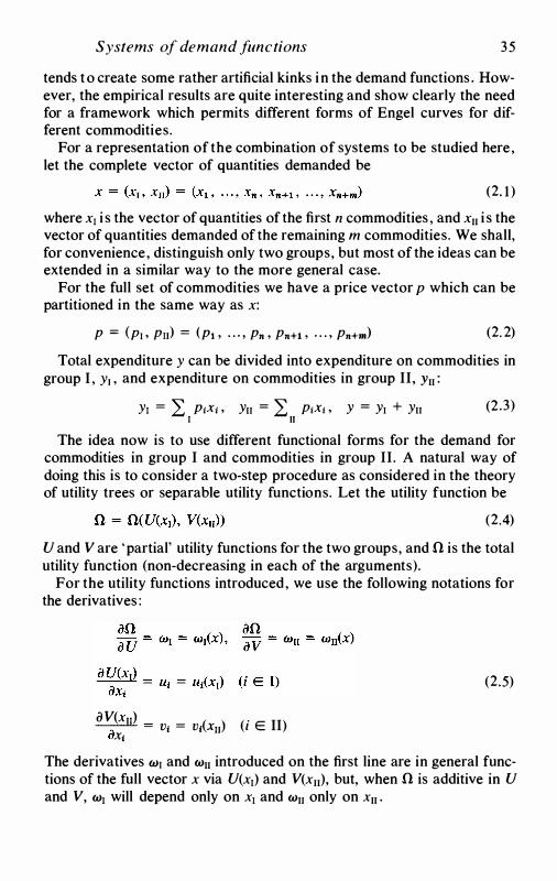
For a representation of the combination of systems to be studied here, let the complete vector of quantities demanded be

(2. 1 )

where xi i s the vector of quantities of the first n commodities , and x11 i s the vector of quantities demanded of the remaining m commodities. We shall, for convenience, distinguish only two groups, but most of the ideas can be extended in a similar way to the more general case.

For the full set of commodities we have a price vector p which can be partitioned in the same way as x:

P = (Pi . Pu) = (Pi , · · · , Pn , Pn+t , · · · , Pn+m) (2. 2)

Total expenditure y can be divided into expenditure on commodities in group I , Yi . and expenditure on commodities in group II, y11 :

Yi = � P;X; , Yn = � P;X; , Y = Yi + Yn (2 .3) i II

The idea now is to use different functional forms for the demand for commodities in group I and commodities in group II. A natural way of doing this is to consider a two-step procedure as considered in the theory of utility trees or separable utility functions. Let the utility function be

(2.4)

U and V are 'partial' utility functions for the two groups, and n is the total utility function (non-decreasing in each of the arguments).

For the utility functions introduced, we use the following notations for the derivatives :

aV(x11) -a- = v1 = vbu) (i E II)

Xi

(2.5)

The derivatives wi and w11 introduced on the first line are in general func­tions of the full vector x via U(xi) and V(x11), but, when n is additive in U and V, wi will depend only on xi and w11 only on x11 •

36 L . J O H A N S E N

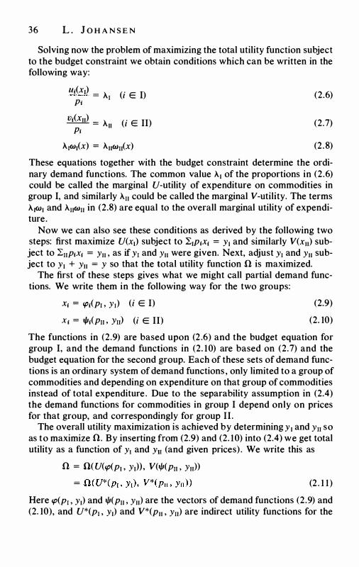
Solving now the problem of maximizing the total utility function subject to the budget constraint we obtain conditions which can be written in the following way:

u;(x1) _ A. - I Pi

vi(xu) _ A. - II Pi

(i E I)

(i E II)

A.1w1(x) = A.uwn(x)

(2.6)

(2.7)

(2.8)

These equations together with the budget constraint determine the ordi­nary demand functions. The common value A.1 of the proportions in (2.6) could be called the marginal U-utility of expenditure on commodities in group I, and similarly A.n could be called the marginal V-utility. The terms A.iW1 and A.nwn in (2.8) are equal to the overall marginal utility of expendi­ture.

Now we can also see these conditions as derived by the following two steps: first maximize U(x1) subject to "L1p1xi = y1 and similarly V(xu) sub­ject to LnPiXi = Yu , as if y1 and Yu were given. Next, adjust y1 and Yu sub­ject to y1 + Yu = y so that the total utility function fi is maximized.

The first of these steps gives what we might call partial demand func­tions. We write them in the following way for the two groups:

xi = 'l'i(Pi . Y1) (i E I)

X1 = l/li(Pn , Yn) (i E II)

(2.9)

(2. 10)

The functions in (2.9) are based upon (2 .6) and the budget equation for group I, and the demand functions in (2. 10) are based on (2.7) and the budget equation for the second group. Each of these sets of demand func­tions is an ordinary system of demand functions , only limited to a group of commodities and depending on expenditure on that group of commodities instead of total expenditure . Due to the separability assumption in (2.4) the demand functions for commodities in group I depend only on prices for that group, and correspondingly for group II.

The overall utility maximization is achieved by determining y1 and Yn so as to maximize n. By inserting from (2.9) and (2. 10) into (2.4) we get total utility as a function of y1 and y11 (and given prices) . We write this as

n = fi( U(ip(pi , Yin. V(l/J(P1i . Yu))

(2 . 1 1 )

Here ip(p1 , y1) and l/J(Pn , Yu) are the vectors of demand functions (2.9) and (2. 10), and U*(p1 , y1) and V*(Pu , Yn) are indirect utility functions for the

Systems of demand functions 37

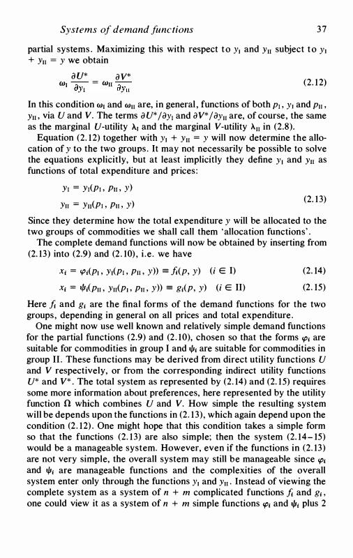
partial systems . Maximizing this with respect to y1 and Yu subject to y1 + Yu = y we obtain

au* av* W1 -!l- = Wu -!l-uY1 uYu (2. 12)

In this condition w1 and wu are, in general , functions of both p1 , y1 and Pu . Yu . via U and V. The terms a U* / ay1 and a V* / ayu are, of course, the same as the marginal U-utility A.1 and the marginal V-utility Au in (2.8).

Equation (2. 12) together with y1 + Yu = y will now determine the allo­cation of y to the two groups. It may not necessarily be possible to solve the equations explicitly, but at least implicitly they define y1 and Yu as functions of total expenditure and prices :

Y1 = Y1(P1 , Pu , y) Yu = Yn(P1 , Pu , y) (2. 13)

Since they determine how the total expenditure y will be allocated to the two groups of commodities we shall call them 'allocation functions' .

The complete demand functions will now be obtained by inserting from (2. 13) into (2.9) and (2 . 10) , i .e . we have

X; = cp;(P1 , Y1(P1 , Pu , y)) = fj(p, y) (i E I)

X; = 1fl;(pu , Yu(Pi . Pu , y)) = g;(p, y) (i E II)

(2. 14)

(2. 15)

Here jj and g; are the final forms of the demand functions for the two groups, depending in general on all prices and total expenditure .

One might now use well known and relatively simple demand functions for the partial functions (2.9) and (2 . 10), chosen so that the forms 'Pi are suitable for commodities in group I and I/Ji are suitable for commodities in group II . These functions may be derived from direct utility functions U and V respectively, or from the corresponding indirect utility functions U* and V* . The total system as represented by (2. 14) and (2. 15) requires some more information about preferences, here represented by the utility function n which combines U and V. How simple the resulting system will be depends upon the functions in (2. 13), which again depend upon the condition (2 . 12) . One might hope that this condition takes a simple form so that the functions (2. 13) are also simple; then the system (2. 14- 15) would be a manageable system. However, even if the functions in (2. 13) are not very simple, the overall system may still be manageable since 'Pi and l/J; are manageable functions and the complexities of the overall system enter only through the functions y1 and Yu . Instead of viewing the complete system as a system of n + m complicated functions jj and g; , one could view it as a system of n + m simple functions cp1 and 1/11 plus 2

38 L. J O H A N S E N

more complicated functions determining y, and y11 • Also, for estimation purposes this way of looking at the system may be practical and conve­nient.

The approach taken here to establishing demand functions bears some relationship to R. A. Pollak's 'conditional demand functions' ( 1969). However, the aims of his study are different. His conditional demand functions for commodities in one group are conditional upon given amounts of commodities in another group. In our context we might try to utilize some of the ideas of Pollak's conditional demand functions for a more general case by abandoning the separability assumption for the util­ity function (2 .4) and formulating our partial demand functions for com­modities in group I, i .e . 'Pi , as conditional upon given amounts of the com­modities in group II, and similarly for the functions I/Ji for group II. In es­tablishing the final form of the complete system, corresponding to (2. 14) and (2. 15), we must then require consistency between the 'given' quan­tities entering as conditions in one set of functions and the decisions about these quantities represented by the other set of functions . This would give a more general approach, but would yield little hope of simple results . I shall therefore retain the assumption of some sort of separability . For this case there is a close connection between the formulas of the following section and formulas in R. A. Pollak ( 197 1a) .

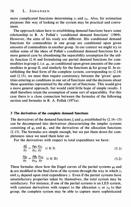
3 The derivatives of the complete demand functions

The derivatives of the demand functions Ji and g; established by (2 . 14- 15) can be decomposed into derivatives characterizing the simpler systems consisting of '(J; and t/J1 , and the derivatives of the allocation functions (2 . 1 3) . The formulas are simple enough, but we put them down for com­pleteness since we need them later on.

For the derivatives with respect to total expenditure we have:

M_ = � iJy, (i E I) ay ay, ay � = � dYn (i E II) iJy iJyn iJy

(3 . 1)

(3.2)

These formulas show how the Engel curves of the partial systems 'Pi and t/11 are modified in the final form of the system through the way in which y1 and Yn depend upon total expenditure y. Even if the partial systems have unsatisfactory properties taken by themselves, the total system may be satisfactory . For instance, if one of the partial systems is an LES system, with constant derivatives with respect to the allocation y1 or y11 to that group, the complete system may be able to capture more sophisticated

Systems of demand functions 39

forms. But , since all demand functions in one group are modified in the same way , all commodities in one group should in a way have the same basic character, for instance all commodities in one group being 'neces­sities ' , or all being 'luxuries' .

The derivatives with respect to prices in the own group are given by

<Jfi = � + � ay1 (i, j E I) ap1 ap1 ay1 ap1 ag1 = � + � � (i, j E II) ap1 ap1 ayu ap1

(3 .3)

(3.4)

The price derivatives of the partial systems are modified by price effects via the allocation functions. These modifications can go in either direction and can make the price derivatives depend in interesting ways upon total income even if the partial systems are too rigid in this sense taken by themselves.

For the price derivatives across groups we have

<Jfi = � <Jy1 (i E I' j E II) ap1 ay1 ap1 <Jg; = � <Jyn (i E II, j E I) <Jp; ayu <Jp;

(3.5)

(3 .6)

These effects assert themselves only through the effects of the price on the total allocation to the group to which the commodity belongs. It ap­pears that the complete system can exhibit both complementarity and alternativity in demand even if the partial systems are too simple to do so. However, if inferiority is ruled out in the partial systems, then all com­modities in one group show the same sort of relation to a particular com­modity in the other group.

4 Additive separability

Let us consider the case where the separability assumption in (2.4) is strengthened to additive separability , i .e .

(4. 1 )

Then the terms w1 and wu in the formulations in section 2 are both equal to unity . The condition determining the allocation functions (2. 1 3) is then

<JU*(P1 , Y1) _ <JV*(pu , Yu) ayl

-ayu (4.2)

The derivatives entering this condition are the same as A.1 and A.11 entering the formulation (2.6-8) of the conditions for utility maximization. Condi-

40 L. J O H A N S E N

tion (4.2) can therefore also be written

ll1(p(pi , Y1)) = V1(1/J(pu , Yu)) (i E I, j E II) P1 P1 (4.3)

Conditions (4.2) or (4.3) are somewhat simpler than the conditions in the general case, in that we have avoided the appearance of all Pi , Pn , Yi , Yn on both sides of the equations. However, the allocation functions will still tend to be rather cumbersome .

Let us explore the working of the system by considering one group of commodities which, within the group, obey the linear expenditure system, and another group which corresponds to a quadratic utility func­tion. We might consider the latter group as a group of necessities , with quadratic utility functions formulated so as to imply a saturation point for each commodity in the group. For the commodities in the group corre­sponding to the linear expenditure system, we should stipulate minimum quantities . For simplicity we omit these parameters ; they could easily be introduced afterwards if we so wish. The total utility function can then be written as

1 1 n = L O'.j In Xj - -2 L -k (c1 - X1)2 I II i

(4.4)

In the second group c1 are the saturation quantities. The utility functions in this group are meant to follow the quadratic curve up to this point, and to be flat from there on. Since the marginal utility is always positive for commodities in the first group, it is clear that a meaningful maximization takes place so that we have x1 < c1 for all commodities in the second group. (We assume all a1 > 0, all k1 > 0, and Lai = 1 . )

The partial system for the first group is now simply

X1 = '1'1(P1 . Y1) = a1 Yi (i E I) Pi

The functions for the second group can be written as

(i E II)

(4.5)

(4 .6)

It should be observed that the Engel functions for both systems are linear. A more general system based on a quadratic utility function, allowing

for interaction terms which we have neglected here, has been studied by A. S. Goldberger ( 1967), and in a dynamic context by H. S. Houthakker and L. D. Taylor ( 1970). The system has also been studied by L. Wegge ( 1968), following up earlier work by H. Houthakker. Houthakker and

Systems of demand functions 4 1

Wegge take into account the non-negativity condition x; � 0 and permit boundary solutions, using a quadratic programming approach. The Engel curves are then kinked linear. We shall neglect this possibility and assume interior solutions. Then (4.6) is valid.

It remains to find the allocation functions. We may proceed according to (4.3) . This yields

__!_ = L11 Ph Ch - Y11 = A _ Yn

y, L khp'j. B II

(4.7)

where we have introduced, for convenience, A and B for the sums en­tering the numerator and the denominator in the middle expression. Com­bining now this with the budget constraint y1 + y11 = y we obtain an equa­tion for y1 which can be solved to give

y, = t {(y - A) + [(y - A)2 + 4B]112} (4.8)

Mathematically there is also a solution with a minus before the square root , but this solution is irrelevant .

When we have the allocation function (4.8) for y1 it follows that the allo­cation to group II will be

1 Yn = - {y + A - [(y - A)2 + 4B]112} 2 (4.9)

For very small values of y, (4.9) will give Yn < 0, which is not mean­

ingful. It is necessary that y > ! . If we had retained the ' minimum quan­

tities' in the LES system for group I this could have turned out dif­ferently, especially if we had permitted them to take negative values.

From these allocation functions it follows that total expenditure on each of the two groups will now increase in a non-linear fashion with total expenditure y. It is seen that if y increases beyond all limits, then y1 will take a dominating part of y , while Yn will take an insignificant share . In fact, we have

y, _ 1 y and YII - 0 when y - oo y (4. 1 0)

In absolute terms Yn - A when y - oo, which agrees with the interpreta­tion of A as the amount necessary to buy the saturation quantities c1 for i E II. We might say that group II as a whole (for y above some limit) be­haves as a necessity, while group I behaves as the remainder must behave according to the budget constraint. This is plausible in view of the fact

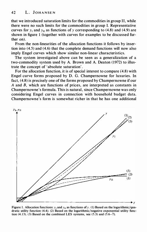
42 L . J O H A N S E N

that we introduced saturation limits for the commodities in group II , while there were no such limits for the commodities in group I. Representative curves for y1 and y11 as functions of y corresponding to (4.8) and (4.9) are shown in figure 1 (together with curves for examples to be discussed fur­ther on) .

From the non-linearities of the allocation functions it follows by inser­tion into (4.5) and (4.6) that the complete demand functions will now also imply Engel curves which show similar non-linear characteristics.

The system investigated above can be seen as a generalization of a two-commodity system used by A. Brown and A. Deaton ( 1972) to illus­trate the concept of 'absolute saturation' .

For the allocation function, it is of special interest to compare (4.8) with Engel curve forms proposed by D. G. Champernowne for luxuries. In fact, (4.8) is precisely one of the forms proposed by Champernowne if our A and B, which are functions of prices, are interpreted as constants in Champernowne's formula. This is natural , since Champernowne was only considering Engel curves in connection with household budget data. Champernowne's form is somewhat richer in that he has one additional

�'""'-������������������������---+ y Figure 1 . Allocation functions: y1 and y11 as functions of y. ( I ) Based on the logarithmic/qua­dratic utility function (4.4). (2) Based on the logarithmic/negative exponential utility func­tion (4. 13). (3) Based on the combined LES systems, see (5.3) and (5.6-7).

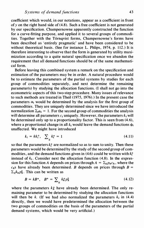
Systems of demand functions 43

coefficient which would, in our notations, appear as a coefficient in front of y on the right hand side of (4.8). Such a free coefficient is not generated by our specification. Champemowne apparently constructed the function for a curve-fitting purpose, and applied it to several groups of commodi­ties. Together with the Tomqvist forms, Champemowne's forms have been described as 'entirely pragmatic' and have been considered to be without theoretical basis . (See for instance L. Phlips , 1974, p. 1 12 . ) It is therefore interesting to observe that the form is generated by utility maxi­mization according to a quite natural specification once we abandon the requirement that all demand functions should be of the same mathemati­cal form.

Before leaving this combined system a remark on the specification and estimation of the parameters may be in order. A natural procedure would be to estimate the parameters of the partial systems by studies for each group of commodities separately, and next determine the remaining parameter(s) by studying the allocation functions. (I shall not go into the econometric aspects of this two-step procedure. Many issues of relevance to such methods are treated in Theil ( 1975, 1976). ) In the present case the parameters a1 would be determined by the analysis for the first group of commodities. They are uniquely determined since we have introduced the normalization 2:1ai = l . For the second group of commodities the analysis will determine all parameters c1 uniquely . However, the parameters k1 will be determined only up to a proportionality factor. This is seen from (4.6), where a proportional change in all k1 would leave the demand functions l/11 unaffected. We might have introduced

k; = kkt , :L kt = 1 (4. 1 1) II

so that the parameters kt are normalized so as to sum to unity. Then these parameters would be determined by the study of the second group of com­modities , and the demand functions given in (4.6) could be written with kt instead of k1 • Consider next the allocation function (4.8). In the expres­sion for this function A depends on prices through A = 2:uphch , where the chs have already been determined. B depends on prices through B = 2:ukhp� . This can be written as

B = kB*, B* = L kit p� II

(4. 12)

where the parameters k� have already been determined. The only re­maining parameter to be determined by studying the allocation functions will then be k. (If we had also normalized the parameters k1 in (4.4) directly , then we would have predetermined the allocation between the two groups of commodities on the basis of the parameters of the partial demand systems, which would be very artificial .)

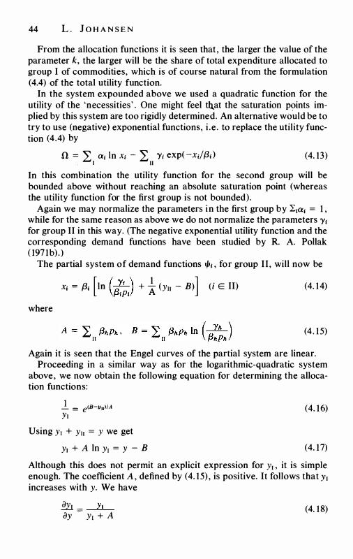
44 L . J O H A N S E N

From the allocation functions it is seen that , the larger the value of the parameter k, the larger will be the share of total expenditure allocated to group I of commodities, which is of course natural from the formulation (4.4) of the total utility function.

In the system expounded above we used a quadratic function for the utility of the 'necessities' . One might feel tb.at the saturation points im­plied by this system are too rigidly determined. An alternative would be to try to use (negative) exponential functions, i .e. to replace the utility func­tion (4.4) by

n = L O'.j In Xj - L Yi exp(-x;//3;) I II

(4. 13)

In this combination the utility function for the second group will be bounded above without reaching an absolute saturation point (whereas the utility function for the first group is not bounded).

Again we may normalize the parameters in the first group by L1a1 = 1 , while for the same reason as above we do not normalize the parameters Y1 for group II in this way. (The negative exponential utility function and the corresponding demand functions have been studied by R. A. Pollak ( 197 1b).)

The partial system of demand functions l/J1 , for group II, will now be

where

X1 = /31 [tn (/3��) + l (y11 - B)] (i E II) (4. 14)

(4 . 15)

Again it is seen that the Engel curves of the partial system are linear. Proceeding in a similar way as for the logarithmic-quadratic system

above, we now obtain the following equation for determining the alloca­tion functions:

_!_ = e<B-1111)/A Yi

Using y1 + y11 = y we get

Yi + A In Y1 = y - B

(4. 16)

(4. 17)

Although this does not permit an explicit expression for y1 , it is simple enough. The coefficient A , defined by (4. 15) , is positive. It follows that Yi increases with y. We have

CJy1 _ _ Y_1_ CJy - Yi + A (4. 18)

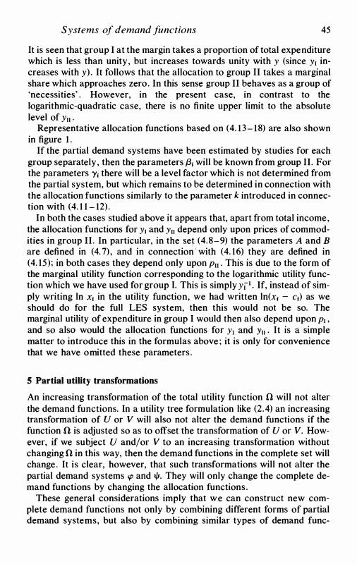
Systems of demand functions 45

It is seen that group I at the margin takes a proportion of total expenditure which is less than unity, but increases towards unity with y (since Yi in­creases with y) . It follows that the allocation to group II takes a marginal share which approaches zero. In this sense group II behaves as a group of 'necessities' . However, in the present case, in contrast to the logarithmic-quadratic case, there is no finite upper limit to the absolute level of Yn .

Representative allocation functions based on (4. 1 3- 18) are also shown in figure 1 .

If the partial demand systems have been estimated by studies for each group separately , then the parameters {31 will be known from group II. For the parameters y1 there will be a level factor which is not determined from the partial system, but which remains to be determined in connection with the allocation functions similarly to the parameter k introduced in connec­tion with (4. 1 1 - 12) .

In both the cases studied above it appears that, apart from total income, the allocation functions for Yi and Yn depend only upon prices of commod­ities in group II. In particular, in the set (4.8-9) the parameters A and B are defined in (4. 7) , and in connection ' with (4. 16) they are defined in (4. 15); in both cases they depend only upon Pn . This is due to the form of the marginal utility function corresponding to the logarithmic utility func­tion which we have used for group I. This is simply y(1 • If, instead of sim­ply writing In x1 in the utility function, we had written ln(x1 - c1) as we should do for the full LES system, then this would not be so. The marginal utility of expenditure in group I would then also depend upon Pi , and so also would the allocation functions for Yi and Yn . It is a simple matter to introduce this in the formulas above ; it is only for convenience that we have omitted these parameters .

5 Partial utility transformations

An increasing transformation of the total utility function 0 will not alter the demand functions. In a utility tree formulation like (2.4) an increasing transformation of U or V will also not alter the demand functions if the function 0 is adjusted so as to offset the transformation of U or V. How­ever, if we subject U and/or V to an increasing transformation without changing 0 in this way, then the demand functions in the complete set will change. It is clear, however, that such transformations will not alter the partial demand systems cp and l/J. They will only change the complete de­mand functions by changing the allocation functions .

These general considerations imply that we can construct new com­plete demand functions not only by combining different forms of partial demand systems, but also by combining similar types of demand func-

46 L . J O H A N S E N

tions fot both groups. For instance, consider again the simplified linear expenditure system. We now assume this system to be valid for both groups. If we have a utility function

n = L a; In X; + L a; In X; I II (5. 1)

then both the partial systems as well as the complete system would be LES systems. However, if we subject one or both parts of the total utility function to increasing transformations by

n = F1 (L I a; In x;) + Fu (L il a; In x;) (5 . 2)

where F1 and Fu (or at least one of them) are increasing, non-linear func­tions, then both the partial systems will still be LES systems, while the complete system will be of a different form. In particular, the Engel curves will no longer be linear. Since the LES system is so convenient to handle and in some respects also empirically successful, but at the same time not quite satisfactory especially with regard to the Engel curve as­pects, a formulation like (5.2) may give rise to an extended range of appli­cability of demand analysis on the basis of LES functions.

As an example of (5 . 2) one might use the antilogarithm for the transfor­mation F1 • This gives

n n = k TI x'f; + L a; In X; (5.3)

i=l II The first part of this formula also corresponds to a usual way of writing the utility function underlying the LES system. In this formulation we may have the normalizations L1a; = 1 and Lua; = 1 .

We now have

(5.4)

X; = "11(Pu , Yu) = a; Yu (i E II) P1

Using these as in connection with (4. 1 -3), with U corresponding to the first part of (5. 3) and V corresponding to the second part, we obtain an equation for the allocation functions which gives the following value for Yu :

Yu = k-1 TI (!!1)°'' j=l O'.j (5.5)

y1 is then y minus the expression (5.5) for y11 • This is a rather strange case, with Yu independent of total expenditure y, but depending upon the prices

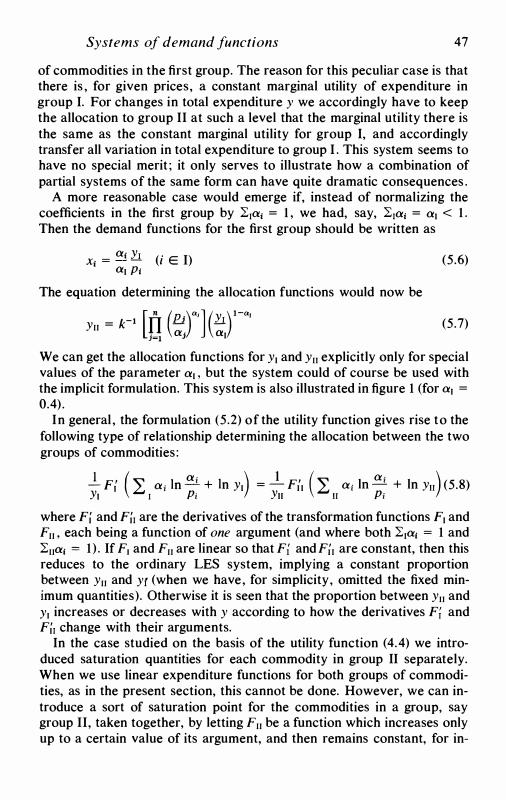
Systems of demand functions 47

of commodities in the first group. The reason for this peculiar case is that there is , for given prices, a constant marginal utility of expenditure in group I. For changes in total expenditure y we accordingly have to keep the allocation to group II at such a level that the marginal utility there is the same as the constant marginal utility for group I, and accordingly transfer all variation in total expenditure to group I . This system seems to have no special merit ; it only serves to illustrate how a combination of partial systems of the same form can have quite dramatic consequences .

A more reasonable case would emerge if, instead of normalizing the coefficients in the first group by Lia1 = 1 , we had, say, Lia1 = ai < 1 . Then the demand functions for the first group should be written as

X1 = ai Yi (i E I) ai P1

The equation determining the allocation functions would now be

_ [ n (p1)"';] (Yi) i-a:, Yu = k 1 IT - -j=l O'.j O'.i

(5.6)

(5.7)

We can get the allocation functions for Yi and Yu explicitly only for special values of the parameter ai , but the system could of course be used with the implicit formulation. This system is also illustrated in figure 1 (for ai = 0.4) .

In general , the formulation (5.2) of the utility function gives rise to the following type of relationship determining the allocation between the two groups of commodities :

J__ F{ ( L a; In a; + In Yi) = _l_ F{i ( L a; In a; + In Yn) (5.8) Yi i Pi Yn n P; where Fl and Fli are the derivatives of the transformation functions Fi and Fu , each being a function of one argument (and where both L1a1 = 1 and Lua1 = 1 ) . If F, and Fu are linear so that Fl and Fl1 are constant, then this reduces to the ordinary LES system, implying a constant proportion between Yu and yf (when we have, for simplicity, omitted the fixed min­imum quantities). Otherwise it is seen that the proportion between Yu and y, increases or decreases with y according to how the derivatives Fl and Fli change with their arguments.

In the case studied on the basis of the utility function (4.4) we intro­duced saturation quantities for each commodity in group II separately. When we use linear expenditure functions for both groups of commodi­ties, as in the present section, this cannot be done. However, we can in­troduce a sort of saturation point for the commodities in a group, say group II, taken together, by letting Fu be a function which increases only up to a certain value of its argument, and then remains constant, for in-

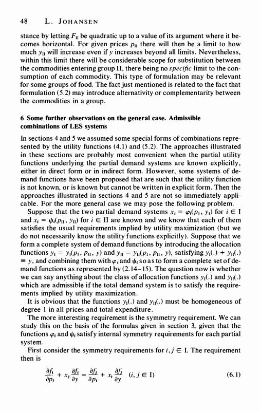
48 L . J O H A N S E N

stance by letting Fu be quadratic up to a value of its argument where it be­comes horizontal . For given prices Pu there will then be a limit to how much Yu will increase even if y increases beyond all limits . Nevertheless, within this limit there will be considerable scope for substitution between the commodities entering group II, there being no specific limit to the con­sumption of each commodity. This type of formulation may be relevant for some groups of food. The fact just mentioned is related to the fact that formulation (5.2) may introduce altemativity or complementarity between the commodities in a group.

6 Some further observations on the general case. Admissible combinations of LES systems

In sections 4 and 5 we assumed some special forms of combinations repre­sented by the utility functions (4. 1 ) and (5 .2) . The approaches illustrated in these sections are probably most convenient when the partial utility functions underlying the partial demand systems are known explicitly , either in direct form or in indirect form. However, some systems of de­mand functions have been proposed that are such that the utility function is not known, or is known but cannot be written in explicit form. Then the approaches illustrated in sections 4 and 5 are not so immediately appli­cable . For the more general case we may pose the following problem.

Suppose that the two partial demand systems x; = cp;(p, , y,) for i E I and x; = 1/J;(pu , Yu) for i E II are known and we know that each of them satisfies the usual requirements implied by utility maximization (but we do not necessarily know the utility functions explicitly) . Suppose that we form a complete system of demand functions by introducing the allocation functions Y1 = YlPi . Pu . y) and Yu = Yu(p, , Pu . y), satisfying y,( . ) + Yu( . ) = y, and combining them with cp ; and ljl; so as to form a complete set of de­mand functions as represented by (2. 14- 15). The question now is whether we can say anything about the class of allocation functions y,( . ) and Yu( .) which are admissible if the total demand system is to satisfy the require­ments implied by utility maximization.

It is obvious that the functions y1( . ) and Yu( . ) must be homogeneous of degree 1 in all prices and total expenditure .

The more interesting requirement is the symmetry requirement. We can study this on the basis of the formulas given in section 3, given that the functions cp; and ljl; satisfy internal symmetry requirements for each partial system.

First consider the symmetry requirements for i ,j E I. The requirement then is

af; + x af; = afj + x·

afj (i, j E I) ap1 1 ay ap; • ay (6. 1)

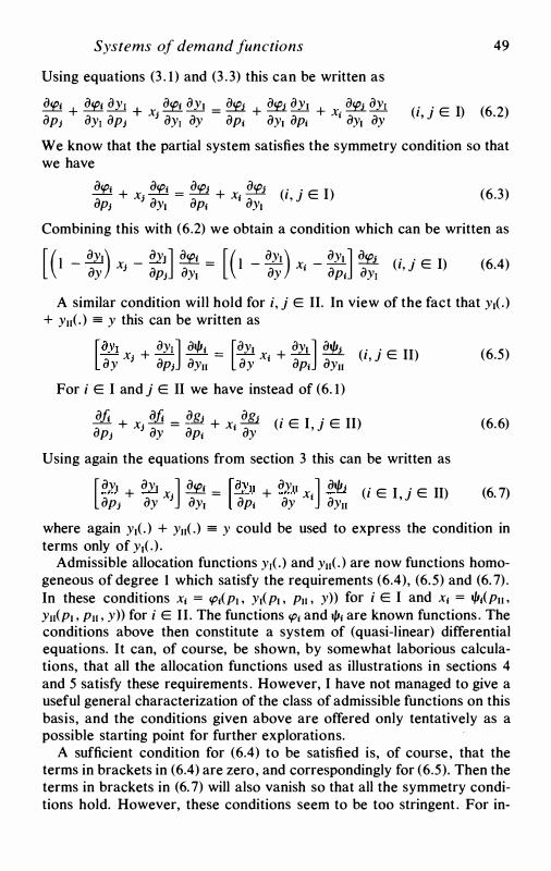
Systems of demand functions 49

Using equations (3 . 1 ) and (3 . 3) this can be written as

� + � dY1 + Xj � dY1 = � + � dY1 + X· iJ.!£1- dY1 dPJ dY1 dPJ iJyi iJy iJp; iJy1 iJp; ' c"Jy1 iJy (i, j E I) (6·2)

We know that the partial system satisfies the symmetry condition so that we have

iJcp; + x iJcp; = E.!£1. + x E.!£1. (i . E I) iJpJ J c"Jy1 iJp; 1 c"Jy1 ' J (6.3)

Combining this with (6.2) we obtain a condition which can be written as

[ ( l _ dYi) x _ c"Jy1J � = [( l _ iJyi ) x· _ c"Jy1 J � (i . E I) iJy J iJpJ c"Jy1 iJy ' c"Jp; c"Jy1 , J (6.4)

A similar condition will hold for i, j E II. In view of the fact that y1( .) + Yu(. ) = y this can be written as

[dY1 Xj + dY1] dt/J; = [dY1 X; + dY1 ] � (i, j E II) (6.5) iJy iJpJ iJyu iJy iJp; iJyu For i E I and j E II we have instead of (6. 1)

c"Jjj + x ajj = iJgJ + x � (i E I j E II) (6.6) dPJ J iJy iJp; ; iJy ' Using again the equations from section 3 this can be written as

[ iJY1 + c"Jy1 xJ] � = [iJYu + c"Jyu x;] iJtfJJ (i E I , j E II) (6. 7) iJpJ iJy iJY1 iJp; iJy iJyu where again y1( . ) + Yu( .) = y could be used to express the condition in terms only of Y1( .) .

Admissible allocation functions y1( .) and Yu( . ) are now functions homo­geneous of degree 1 which satisfy the requirements (6.4), (6.5) and (6. 7) . In these conditions x; = cp;(Pi . y1(p1 , Pu , y)) for i E I and x; = t/11(P1i . Yu(P1 , Pu , y)) for i E II. The functions cp; and 1/11 are known functions . The conditions above then constitute a system of (quasi-linear) differential equations. It can, of course, be shown, by somewhat laborious calcula­tions, that all the allocation functions used as illustrations in sections 4 and 5 satisfy these requirements . However, I have not managed to give a useful general characterization of the class of admissible functions on this basis, and the conditions given above are offered only tentatively as a possible starting point for further explorations.

A sufficient condition for (6.4) to be satisfied is, of course, that the terms in brackets in (6.4) are zero, and correspondingly for (6.5). Then the terms in brackets in (6. 7) will also vanish so that all the symmetry condi­tions hold. However, these conditions seem to be too stringent . For in-

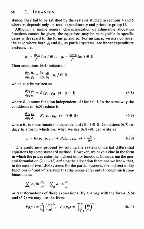
50 L. J O H A N S E N

stance, they fail to be satisfied by the systems studied in sections 4 and 5 where Yi depends only on total expenditure y and prices in group II.

Although a simple general characterization of admissible allocation functions cannot be given, the equations may be manageable in specific cases with regard to the forms cp1 and 1/11 • For instance, we may consider the case where both cp1 and I/It , as partial systems, are linear expenditure systems, i .e.

'Pt = aiYi for i E I, I/It = aiYn for i E II P1 Pi

Then conditions (6.4) reduce to

..m_ at = dYi ':!! (i, j E I) Clp1 Pt dp; P1 which can be written as

dYi Pt - R ( ) ( . E I) -a

- - i Pi . Pn , Y 1 P1 a1 (6.8)

where Ri is some function independent of i for i E I. In the same way the conditions in (6.5) reduce to

aayi Pi = Ru(Pi . Pn ' y) (i E II) Pt at (6.9)

where Rn is some function independent of i for i E II. Conditions (6.7) re­duce to a form, which we, when we use (6. 8-9) , can write as

) Clyi Yi = Ri(pi . Pu . Y + Ru(p, , Pn . y) + ay Y (6. 10)

One could now proceed by solving the system of partial differential equations by some standard method. However, we have a clue in the form in which the prices enter the indirect utility function. Considering the gen­eral formulation (2 . 1 1 - 12) defining the allocation functions we know that, in the case of two LES systems for the partial systems , the indirect utility functions U* and V* are such that the prices enter only through such com­binations as

at ""' at In - , £,,, i Pl a· L a1 In --1

II Pi or transformations of these expressions . By analogy with the forms (5.5) and (5. 7) we may use the forms

n (P•0"; n+m (Pi)"; Pi(p,) = n � ' Pn(Pn) = . TI --; t=l i=n+l (6. 1 1)

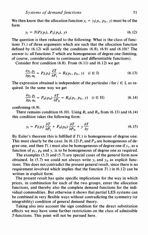
Systems of demand functions 5 1

We then know that the allocation function y1 = y1(p1 , p11 , y) must be of the form

(6. 12)

The question is then reduced to the following: What is the class of func­tions T( .) of three arguments which are such that the allocation function defined by (6. 1 2) will satisfy the conditions (6. 8), (6.9) and (6. 10)? The answer is: all functions T which are homogeneous of degree one (limiting, of course, considerations to continuous and differentiable functions).

Consider first condition (6.8). From (6. 1 1) and (6. 1 2) we get

�Y1 p; = P1(P1) �PT = R1(Pi . Pu , y) (i E I) up; a; u 1 (6. 1 3)

The expression obtained is independent of the particular i for i E I, as re­quired. In the same way we get iJY1 Pi iJT

-;---- - = Pn(Pn) "P = Ru(Pi . Pu , y) (i E II) up; a; u 11 confirming (6.9) .

(6. 14)

There remains condition (6. 10). Using R1 and R11 from (6. 13) and (6. 14) this condition takes the following form:

iJT iJT iJT Y1 = P1(P1) iJPi + Pn(Pn) iJPn + Y iJy (6. 15)

By Euler's theorem this is fulfilled if T( .) is homogeneous of degree one. This must clearly be the case. In (6. 12) P1 and P11 are homogeneous of de­gree one, and then T( .) must also be homogeneous of degree one if y1 , as a function of p1 , p11 and y, is to be homogeneous of degree one as required.

The examples (5. 5) and (5 .7) are special cases of the general form now obtained. In (5 .7) we could not always write y1 and y11 as explicit func­tions. This does not contradict the present general result, since there is no requirement involved which implies that the function T( .) in (6. 1 2) can be written in explicit form.

The present result has quite specific implications for the way in which prices, in combination for each of the two groups, enter the allocation functions, and thereby also the complete demand functions for the indi­vidual commodities . But otherwise it shows that partial LES systems can be combined in very flexible ways without contradicting the symmetry (or integrability) condition of general demand theory.

Taking also into account the sign condition for the direct substitution effects we may have some further restrictions on the class of admissible T-functions. This point will not be pursued here.

52 L. J O H A N S E N

7 Summary and conclusion

The purpose of this paper has been to explore the possibilities which are opened up for constructing useful systems of demand functions by aban­doning the requirement that the functions for all commodities should be of the same mathematical form. We can then use relatively simple well­known systems for groups of commodities, and use 'allocation functions' for allocating expenditure between the groups of commodities so that overall utility maximization is achieved. The examples developed in sec­tions 4 and 5 show that the approach is feasible and able to yield Engel curves which are more flexible and satisfactory than the Engel curve properties of the partial systems taken each by itself. (Other examples can easily be constructed by combining the varioµs partial systems in dif­ferent ways from those used in sections 4 and 5 . ) I have concentrated on the Engel curve aspects because the Engel curve properties of many of the relatively simple usual systems are known, from empirical studies , to be unsatisfactory. I have used the LES system as a standard example be­cause this system is so convenient and successful in some respects . It is therefore a very attractive candidate for partial systems to be used in the combined total systems, and I think the examples illustrate that this can be a fruitful direction of development and lead to a valuable extension of the scope of application for this system. The results in the last part of sec­tion 6 are especially important in this respect .

Although I have concentrated on the Engel curve properties of the systems, the combinations do, of course, also have implications for the price elasticities . The examples in section 5 show how simple combina­tions can introduce non-additivity in the overall system although each partial system is based on an additive utility function. It would be interest­ing to explore to what extent such simple extensions help to overcome the rather rigid connections between price and income elasticities which have been studied (and criticized) by A. Deaton ( 1974).

There are now available several empirical studies which compare the performance of various systems of demand functions. Some of them are rather inconclusive, while others are more or less contradictory. One reason for this may be that none of the systems is good for all commodi­ties. Summarizing one such study A. P. Barten ( 1977) comments as follows : 'For all groups together, the Rotterdam system is superior to the indirect addilog model, which does better than the LES. The picture is mixed for individual groups, however. For food and beverages and to­bacco, the Rotterdam model is better; for durables, the indirect addilog system dominates the Rotterdam system slightly ; while the LES is clearly outstanding for the remainder. · Such results seem to call for combined systems and lend empirical support to the approach taken in the present paper.

Systems of demand functions 53

Note

I am grateful to Karl Moene for his very valuable assistance in the preparation of this paper, and to Knut Sydsreter for useful discussions on special points.

References

Aitchison, J. and Brown, J. A . C. ( 1954), 'A Synthesis of Engel Curve Theory' , Review of Economic Studies, 22, pp. 35 -46.

( 1963), The Lognormal Distribution, Cambridge University Press, Cambridge . Andersson, A. E. ( 1977), ' Merit Goods and Micro-Economic Dependence' , in A.

J . Culyer and V. Halberstadt (eds . ) , Public Economics and Human Resources , Editions Cujas, Paris, pp. 2 15-36.

Barten, A . P. ( 1977), 'The Systems of Consumer Demand Functions Approach: A Review' , Econometrica, 45, pp. 23 -5 1 .

van Beeck, J . G . and den Hartog, H . ( 1964), 'Consumption Forecasts for the Netherlands' , in J . Sandee (ed.) , Europe's Future Consumption, North­Holland, Amsterdam.

Brown, A. and Deaton, A. ( 1972), 'Surveys in Applied Economics: Models of Consumer Behaviour' , The Economic Journal, 82, pp. 1 145- 1 236.

Carlevaro , F. ( 1974), Sur la comparaison et la generalisation de certains systemes des fonctions de consommation semi-agregees, Herbert Lang, Berne.

( 1976), 'A Generalization of the Linear Expenditure System', in Private and En­larged Consumption (edited by L. Solari and J.-N. Pasquier), North-Holland, Amsterdam.

Champemowne, D. G. ( 1969), Uncertainty and Estimation in Economics. Volume 2, Oliver and Boyd, Edinburgh .

Deaton, A. ( 1 974), 'A Reconsideration of the Empirical Implications of Additive Preferences' , The Economic Journal, 84, pp. 338-48.

Fisk, P. R. ( 1958-59) , 'Maximum Likelihood Estimation of Tornqvist Demand Equations' , Review of Economic Studies, 26, pp. 33-50.

Goldberger, A. S. ( 1967), Functional Form and Utility: A Review of Consumer Demand Theory, Social Systems Research Institute , University of Wisconsin.

Hoflund, 0. ( 1954), 'On the Geometric Structure of Indifference Maps' , Paper presented at the European Meeting of the Econometric Society, Uppsala.

Houthakker, H. S. and Taylor, L. D. ( 1970), Consumer Demand in the United States: Analysis and Projections, Harvard University Press , Cambridge (Mass.) . Second edition.

Keck, A . ( 1968), Nationaleinkommen-Konsumption, Verlag die Wirtschaft, Berlin (GDR).

Lau, L. J. ( 1977), 'Complete Systems of Consumer Demand Functions through Duality' , in M. C. Intriligator (ed .) , Frontiers of Quantitative Economics, Vol . III A, North-Holland, Amsterdam.

McElroy , M. B . ( 1975), 'A Spliced CES Expenditure System', International Eco­nomic Review, pp. 765-78.

Phlips, L. ( 1974), Applied Consumption Analysis, North-Holland, Amsterdam. Pollak, R. A . ( 1969), 'Conditional Demand Functions and Consumption Theory ' ,

Quarterly Journal of Economics, 83, pp. 70-8. ( 1971 a) , 'Conditional Demand Functions and the Implications of Separable Util­

ity' , Southern Economic Journal, 37, pp. 423-33. ( 1971b) , 'Additive Utility Functions and Linear Engel Curves' , Review of Eco­

nomic Studies, 38, pp. 401 - 13 .

54 L . J O H A N S E N

Solari, L . ( 1971 ) , Theorie des choix etfonctions de consommation semi-agregees ­Modeles Statiques, Librarie Droz, Geneva and Paris.

Somermeyer, W. H. and Langhout , A . ( 1972), ' Shapes of Engel Curves and De­mand Curves: Implications of the Expenditure Allocation Model, Applied to Dutch Data' , European Economic Review, pp. 351 -86.

Stone, J. R. N. ( 1954), 'Linear Expenditure Systems and Demand Analysis: An Application to the Pattern of British Demand' , The Economic Journal, 64, pp. 5 1 1 -27.

Theil, H. ( 1975 , 1976) Theory and Measurement of Consumer Demand, two vol­umes, North-Holland.

Valtukh, K. K. ( 1975), ·A Theoretical Model of Mass Consumer Behavior and some Methodological Problems of Social Studies' , Quantity and Quality .

Varian, H. R. ( 1978), 'A Note on Locally Constant Income Elasticities' , Econom­ics Letters, pp. 9-13 .

Wegge, L. L. ( 1968), 'The Demand Curves from a Quadratic Utility Indicator' , Review of Economic Studies, 35, pp. 209-24.

Wold, H. ( 1952), in association with L. Jureen, Demand Analysis, Almquist and Wiksell, Stockholm, and Wiley, New York.

3 Theoretical and empirical

approaches to consumer demand

under rationing1

A N G U S D E AT O N

It is a matter of common observation that the quantities consumed of many goods and services are not directly under the control of those who consume them. The level of provision of public goods cannot be varied to taste by any single consumer: shortages or formal rationing of market goods may place an upper limit on consumption: transactions costs or market imperfections , particularly in asset markets, may prevent the short-run adjustment of stocks to their optimum levels so that consumers may have to consume too much as well as too little. Perhaps most impor­tantly, involuntary unemployment in the labour market can be thought of as an enforced consumption of an undesirably large amount of leisure. All these situations involve quantity constraints on consumer behaviour, and although rationing is only one possibility, we shall use the term to deal with all , including those situations where more is consumed than would be freely bought.

As one might expect, much of the early work on rationing was done during and immediately after the second world war. This work is sur­veyed in the classic paper by Tobin ( 1952). For a considerable period sub­sequently , there appeared to be little interest in the subject and little was published, although see the two papers by Pollak ( 1969; 1971) . In the last few years, however, rationing has once again become a major focus of attention. On this occasion the impetus has come, not from the policy issues raised by actual rationing, but from theorists constructing general equilibrium models in which markets are not assumed to clear. In such a world, some buyers and sellers will go short or long and these quantity constraints will have repercussions in other markets. The analysis of these interactions is an exercise in rationing theory and the properties of such equilibria depend upon the properties of demand and supply func­tions under rationing. For further discussions of this literature, see Barro and Grossman ( 1976), Malinvaud ( 1 977) or Muellbauer and Portes ( 1978).

In this paper, I shall be concerned with alternative approaches to deriving rationed demand functions which are suitable for empirical im-

55

56 A . S . D E A T O N

plementation. In particular, I wish to illustrate how duality theory can be used to generate empirically estimable demand functions under rationing in the same way that it can do so in the unrationed case and with the same benefits (see Deaton, 1978). I also deal with the practically important case where one needs a 'matched' pair of demand functions, one rationed and one unrationed, each deriving from the same preferences. Such functions are necessary if we wish to predict behaviour under rationing when we have only observations on free demand (e.g. if an unprecedented shortage occurs) and can sometimes even be used in the converse situation, of pre­dicting unrationed from rationed demands. Similarly, we may wish to esti­mate a system of consumer demand and labour supply functions on a cross-section of households , some of which are rationed (e.g. in the la­bour market) and some of which are not. Such functions can only be esti­mated efficiently if common preferences with common parameters are as­sumed for all households so that the same parameters appear in both sets of demand functions corresponding to the two 'regimes' . The theory of this construction is discussed in section 1 ; it is a fuller version of the re­sults sketched in chapter 4, section 3 of Deaton and Muellbauer ( 1980a) , results independently derived by Neary and Roberts ( 1980). Section 2 presents a simple empirical example in which it is assumed that con­sumers' expenditure on housing in Britain is predetermined in the short run and a model embodying this assumption is contrasted with a more conventional specification in which housing and other expenditures are simultaneously determined. Section 3 discusses the specification of 'flex­ible functional form' models under rationing. For many purposes, empiri­cal models with matched rationed and unrationed demands will yield functional forms which are too restrictive. It is thus important to have general models to incorporate rationing and I discuss a modification to the AIDS (Almost Ideal Demand System) of Deaton and Muellbauer ( 1980b) which permits ration levels to appear in a simple, theoretically satisfac­tory, and empirically tractable manner. Such a formulation also offers an elegant choice-theoretic foundation for the introduction of stocks into de­mand functions. Finally, the extended AIDS is applied to the housing ex­ample considered in section 2. Section 4 is a summary with conclusions .

1 The specification of rationed and unrationed demands

In order to keep the exposition as simple as possible, I shall consider only the case of a single rationed good (at least until section 3 below). The re­sults can straightforwardly be extended to the case of multiple constraints while the analysis for a single good does not require the use of matrix algebra. Let q0 , good zero, be the good to be constrained, while q1 , q2 ,

Consumer demand under rationing 57

. . . , qn , or q, is the vector of unconstrained goods. Hence, if z is the level to which q0 is constrained, the two problems, rationed and unrationed, are given by

max u = v(qo, q) s.t . p0qo + p.q = x

max u = v(q0, q) s.t. Poqo + p.q = x} and q0 = z

( 1 )

(2)

where Po and p are the prices of q0 and q, x is total outlay, u is the utility level, and v(q0, q) is the utility function. To save complications, I assume that this latter has all the standard properties , i .e . it is a strictly quasi­concave, differentiable and increasing function of its arguments . Problem ( 1) has solutions in the normal way, for i = 0, . . . , n ,

q1 = gi(x, po , p) (3)

while for (2), we write , for i = 1 , .. . , n

q1 = gf(x, z , Po . p) (4)

The questions to be discussed are (a) the relationship between (3) and (4),

(b) the properties of (4), (c) suitable functional forms for (4). Consider first the important special case where preferences are weakly

separable between q0 and q - see Pollak ( 1971) . Under separability, v(qo, q) can be written in the form v*(q0, cf>(q)) say, so that (2) can be written, after substitution of z for q0 as

max u = v*{z , cf>(q)} s.t . p.q = x - p0z (5)

The z in v*( ) is essentially irrelevant; problem (5) is clearly identical to the maximization of cf>(q) subject to total outlay corrected for the cost of the ration. The rationed demand functions (4) are thus, i = 1 , . . . , n

q1 = gf(x, z, Po , p) = Ji(x - PoZ , p) (6)

for suitable functions Ji( ) satisfying all the usual properties of demand functions. Hence, under weak separability, the ration level has income ef­fects only and, provided income is corrected for the cost of the ration, the demands for unrationed goods can be dealt with in the usual way. For many goods, particularly public goods, this will provide a satisfactory so­lution. Once I have paid my taxes for my share of the defence budget, that is the end of the matter and I am unlikely to attempt to make up for a cut in the national defence budget by substituting guns for butter in my pri­vate consumption pattern.

In general, however, we cannot suppose that preferences are weakly separable between rationed and unrationed goods . In particular, if leisure

58 A . S . D E A T O N

is being rationed, there are clearly a number of goods and services the de­mand for which cannot be explained in terms of income alone without ref­erence to the number of hours worked. In principle , problem (2) can be solved for any specification of v(q0, q) and the demand functions (4) esti­mated. However, just as in the unrationed case (see Deaton ( 1978) for a full discussion), such problems rarely have explicit solutions in interesting cases and , even when they do, empirical analysis is hampered by the lack of a clear relationship between the demands and the direct representation of preferences . It is also difficult to characterize the rationed demands in rela­tion to the unrationed demands from consideration of the direct utility func­tion. The classic treatment is that of Tobin and Houthakker ( 195 1 ) who manipulate the first-order conditions for (2) to obtain properties of the derivatives of the rationed demands (4). Similarly , they obtain locally valid relationships between the derivatives of the rationed and unrationed functions, for example, the Le Chatelier result - see Samuelson ( 1947) -

that, at the point where the ration would have been bought anyway, com­pensated price rises cause no greater falls in demand under rationing than without it. Such results are of great importance but are insufficient if we require characterizations of the demands themselves rather than only their derivatives. These problems can be solved by following a dual ap­proach.

Begin by defining, for unrationed demands, the consumer' s cost func­tion

c(u, Po, p) = min {poqo + p.q; v(q0, q) � u} qo,q (7)

The cost-minimizing q0 and q in (7) give the Hicksian demand functions corresponding to the Marshallian demands (4). For the rationed situation, exactly analogously, define the rationed cost function

c*(u, p0, p, z) = min {p0z + p.q; v(z , q) � u} (8) q

so that c*(u, p0 , p, z) is the minimum cost of reaching u at p0 and p, given that z of good 0 must be bought. Since the only function of z in (8) is to restrict choice compared with (7), we have at once

c(u , p0 , p) = min c*(u, p0 , p, z) (9) z

This equation is the envelope property illustrated in figure 1 ; the unre­stricted cost function is the inner envelope of the four restricted cost func­tions, each indexed on a particular value of z . Note that since the degree of concavity of the cost function gives the size of the own-price substitu­tion effect, figure 1 is the basis for the Le Chatelier principle .

It is clear that (8) may be rewritten

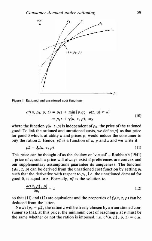
Consumer demand under rationing

cost

c ( u, Po, p)

Figure l . Rationed and unrationed cost functions

c*(u, Po. p, z) = p0z + min {p.q ; v(z , q) � u} q

= PoZ + y(u, z , p) , say

59

( 10)

where the function y(u, z , p) is independent of p0 , the price of the rationed good. To link the rationed and unrationed costs , we define pt as that price for good 0 which, at utility u and prices p, would induce the consumer to buy the ration z . Hence, pt is a function of u, p and z and we write it

pt = �o(u, z , p) ( 1 1)

This price can be thought ofas the shadow or ' virtual' - Rothbarth ( 1941 ) - price of z ; such a price will always exist if preferences are convex and our supplementary assumptions guarantee its uniqueness. The function �0(u, z, p) can be derived from the unrationed cost function by setting p0 such that the derivative with respect to p0 , i .e . the unrationed demand for good 0, is equal to z . Formally, pt is the solution to

iJc(u, Pt , p) = z iJpo ( 1 2)

so that ( 1 1) and ( 12) are equivalent and the properties of �0(u, z, p) can be deduced from the latter.

Now if p0 = pt , the ration z will be freely chosen by an unrationed con­sumer so that, at this price, the minimum cost of reaching u at p must be the same whether or not the ration is imposed, i .e. c*(u, pt , p, z) = c(u,

60 A . S . D E A T O N

p� , p). Hence, from ( 10) and ( 1 1) , as an identity in u, p and z , c{u, g0(u, z , p) , p} = z .g0(u , z , p) + y(u, z , p) ( 13)

Finally , y(u, z , p) can be eliminated between ( 10) and ( 13) to give the de­sired relationship between rationed and unrationed cost functions ,

c*(u , Po , p, z) = {p0 - g0(u, z, p)}z + c{u, g0(u, z , p), p} ( 14)

where, rewriting ( 1 1) and ( 12) , g0 is implicitly defined by

ac{u, go(u, z , p) , p} = z

ilpo ( 15)

Equations ( 14) and ( 15) are the central results of the theory of demand under quantity restrictions and the other results I shall need follow directly from them. By differentiating ( 14) singly and doubly with respect to p and z, rationed and unrationed demands can be compared globally and the effects of ration levels on unrationed demands traced. I shall not discuss these results here, partly because an excellent presentation is already available in Neary and Roberts ( 1980), but principally because my main purpose here is to show by illustration how ( 14) and ( 15) may be used in practice to provide empirically estimable rationed and unrationed demand functions. Two different approaches are followed in the next two sections.

2 A matched pair of rationed and unrationed demands

The implementation of the foregoing theory requires selection of a spe­cific cost function. The main consideration in making a choice in the present context is to ensure that equation ( 15) , defining the virtual price of the ration, should have a specific solution. Consider the class of cost func­tions defined by Muellbauer ( 1981 ) in the context of labour supply . This may be written

c(u, Po, p) = u p8{a(p)}1-a + b(p) Po + d(p) ( 16)

where a(p) and d(p) are linearly homogeneous functions of p, b(p) is a zero-degree homogeneous function of p and 8 E (0, 1) is a parameter. The cost minimizing consumer will equate total expenditure x to c(u, p0, p) so that

x = u p8 {a(p)}1-a + b(p) Po + d(p) ( 17)

can be used to give the indirect utility function, i .e . u as a function of x, p0 and p. In the labour supply context as discussed by Muellbauer, p0 is the wage rate and x must be interpreted as 'full' income, i .e . unearned income plus the value of the time endowment. For a fuller analysis of this and

Consumer demand under rationing 6 1

similar models i n the rationing context see Deaton and Muellbauer ( 1981) . For the present there is no need to tie the interpretation of ( 16) and ( 17) to this particular case although note that, if good 0 is on a par with the other goods in the unrationed case, the cost function treats it asymmetri­cally (although this depends on the choice of the functions a(p), b(p) and d(p)) .

The unrationed demand functions can be derived by differentiating ( 16) with respect to p0 and Pi in turn, using ( 17) to substitute for u. The results are

p0q0 = 8{x - d(p)} + ( 1 - 8)pob(p) ( 1 8)

q1 = {a(p)}-1a;(p)(l - 8){x - p0b(p) - d(p)} + p0b;(p) + d;(p) ( 19)

where ai(p), b1(p) and di(p) are the ith partial derivatives of a(p), b(p) and d(p). In the labour supply context, these functions are particularly attrac­tive because, in a cross-section of households, a1(p), b1(p), d1(p), a(p), b(p) and d(p) are constant, so that both p0q0 and qi are modelled as linear func­tions of x and p0• To derive the rationed demands, we first equate iJc/ iJp0 to z to derive the virtual price function g0(u, p0, p). Hence,

z = 8up&-1{a(p)}1-6 + b(p)

so that ( 1 1) becomes

pt = a(p){8u/(z - b(p))}110-a>

(20)

(2 1)

Note that pt is linear homogeneous in p and non-increasing in z ; a check with ( 15) shows these to be quite general properties of g0(u, p0, p). Substi­tution of (2 1 ) and ( 16) for the general expressions in ( 14) yields the ra­tioned cost function c*(u, p0 , p, z), i .e .

c*(u, Po, p, z) = PoZ + d(p) + (8-1 - l)(8u)110-M(z - b(pW61<1-Ma(p) (22)

or, more compactly , writing u* = (8-1 - l )(8u)110-6>, and p = 8/( 1 - 8) c*(u, Po, p, z) = p0z + d(p) + a(p)u*(z - b)-P (23)

These two equations , (22) and (23), are thus the exact representations of preferences under rationing when ( 16) is the representation without it. Note that, since p > 0, c*(u, p0, p, z) is convex in z, a result which follows quite generally from the quasi-concavity of the direct utility function v(q0 , q), see section 3 below.

The rationed demand functions for q can be derived from (22) or (23) in the usual way. Hence, with q0 set to z , we have, for i = 1 , . . . , n ,

* _ {ai(P) pb;(p) } q1 - d1(p) + a(p) + z _ b(p) {x - PoZ - d(p)} (24)

62 A . S . D E A T O N

The comparison between ( 19) and (24) is instructive. The ration quantity z modifies the original demands in two ways . In the first, x is reduced by PoZ to take account of the cost of the ration; this adjustment would take place even if preferences were separable between rationed and unrationed goods. The second modification is to the marginal propensity to consume of each good. In ( 19) , iJ(p1q1)/ax is ( 1 - 8). a log a/a log p1• However, in (24) , the ( 1 - 8) becomes unity (since good 0 is now replaced by z) and there is the additional term pp;b1(p)/{z - b(p)}. This latter shows how changes in z affect the marginal propensity to spend on the other goods. In this particular case b;(p) > 0 implies that increases in z decrease the marginal propensity to spend on good i, with the reverse if b1(p) < 0 (re­call that "'2:-pkbk(p) = 0 by homogeneity) . These effects are the additional effects of the ration on the pattern of commodity demands given that pref­erences are not separable. It is easily shown that a necessary and suffi­cient condition for ( 16) to represent separable preferences is that b1(p) = 0 for all i, so that the additional effects of the ration on the marginal pro­pensities to spend vanish if and only if preferences are weakly separable between q0 and q.

The most obvious application of the matched rationed and unrationed demands ( 1 8) , ( 19) and (24) is to cross-section data where, for example, some households are free to vary their hours of work while others are either involuntarily unemployed or must work fixed hours. Since the same parameters appear in both rationed and unrationed regimes, fully efficient estimation is possible while, on the other hand, suitable data would allow a test of the theory ofrationing as incorporated in the three equations. For the present, I take a more straightforward example based on time-series data. In a world in which there are imperfect secondhand markets for durable goods, so that there are differences between buying and selling prices or there are major transactions costs, the stocks of durable goods inherited from the past are effectively fixed in the short run, at least for many households . This is particularly true for the stock of housing and, although a minority of consumers can and do adjust their housing in any one year, the majority remain in houses which are too small or too large relative to their current needs and circumstances rather than face the heavy transactions costs and disturbance of moving. If housing expendi­ture were fixed for all households, the rationed model would be the appro­priate one and in the experiments which follow I compare this extreme position with that usually adopted, which treats housing expenditure as a category of consumers' expenditure subject to the same laws as , say, food or services.

As a measure of the ration level for housing, I adopt the definition of current expenditure on housing given in the National Income and Expenditure Blue Books. This includes three principal elements: rents,

Consumer demand under rationing 63

both actual and imputed, which are ideally the flows corresponding to the actual stocks ; rates and water charges, which are essentially taxes over which the consumer has no control but which yield local services ; and household maintenance and repairs , again a largely necessary payment, given the stock in existence. Over none of these elements do consumers have direct short-run control , while together they yield a flow of services which will be substitutable or complementary to other consumption flows. In principle, the stock of any durable could be treated as the ration level itself, and this offers a theoretically satisfactory way of introducing the influence of such stocks into demand functions. However, given the availability of flow data in the current instance, it seems appropriate to use it.

To apply the models based on ( 16) to time-series data where the prices of the non-rationed goods vary, it is necessary to give specific functional forms to the three functions a(p), b(p) and d(p). Consider the following:

n a(p) = aJip�•; 2 ak = 1

1 n b(p) = 'Yo + f3ollp�•; 2 f3k = 0

n d(p) = 2 'YkPk

1

(25)

where a0, . . . , an, {30, . . . , f3n and y0, . . . , 'Yn are parameters to be estimated. It may easily be checked that, as required, a(p) and d(p) are homoge­neous of degree one and b(p) of degree zero. The unrationed and rationed demands ( 1 8), ( 19) and (24) can now be derived; these give

Poqo = Po'Yo + Pof3Jlp�• + 8(x - 'YoPo - 'Y·P - Pof3ollp�) (26)

P1q; = P1'Y; + f31Pof30Ilp�• + ( 1 - 8)ai(x - 'YoPo - 'Y·P - Pof3ollp�) (27)

for the unrationed demands for housing and for other goods, while , in the rationed case, the functions for the unrationed goods are

* ( /3tP/3oil�· ) Piq; = Pi'Yi + a1 + z _ 'Yo _ f3ollp�• (x - 'Y·P - zpo) (28)

where p = 8/( 1 - 8). Note that when {30 or all of the {3;s are zero, (26) and (27) reduce to Stone's ( 1954) linear expenditure system. To the extent that the {3s are important, housing occupies a special place in the free demands while under rationing, the value of z influences the marginal propensities to consume in (28). Once again, when {3 = 0, the separable linear expen­diture system guarantees that the only effect of z in (28) is the income effect - ZPo ·

To estimate equations (26) to (28), I have used post-war annual British

64 A . S . D E A T O N

data from 1954 to 1974 on seven non-durable expenditure categories plus housing: food; clothing; fuel ; drink and tobacco; transport and com­munication; other goods; services. This means there are 27 parameters in (26) and (27), 25 of which can be freely determined. All of these parame­ters also appear in (28) and, given sufficient variation in the data, all can in principle be identified. Note, in particular that 8, the marginal propensity to spend on housing in the free regime, can be estimated when housing is quantity-constrained. The practical situation is somewhat different, espe­cially if we try to estimate by Full Information Maximum Likelihood (FIML). Consider the attempt to estimate (26) and (27) as a set under the (realistic) assumption of no prior knowledge about the variance­covariance matrix of cross-equation errors . Looking first at (26) alone, the equation contains a total of 17 parameters (y0, {30, f3i. . . . , f31, Yi . . . . , y7, 8) . There are only 2 1 observations and, although these parameters appear in other equations, i t will be possible, at the price of a very poor fit else­where , to obtain an almost perfect fit for (26) alone, or indeed for any other single equation. In FIML estimation, where the determinant of the estimated variance-covariance matrix is being minimized, a perfect fit for one equation guarantees a zero determinant and an infinite log likelihood. Hence, for the data at hand, it is not sensible to try to estimate these models by FIML techniques .

An alternative procedure is to impose prior restrictions on the variance-covariance matrix . For example, if we write wii for E(ut1Ut;) where Utt and Ut; are the errors at time t in equations i andj, then one pos­sibility is to write wii = a-2(8ii - n-1) where 8ii is the Kronecker delta. This leads to estimation by minimizing the total residual sum of squares over all equations (see Deaton, 1975, p. 39). A number of equations were estimated in this way but it became clear that the zero degree price func­tion {30Ilp�k was always close to being constant over the sample . This is to be expected given the collinearity of the prices, but means that, in (26) and (27), it is not possible to identify both {30 and 'Yo while, in (28), in addi­tion, p cannot be identified. It is thus best in practice to accept the approx­imation and rewrite the three equations as

Wo = royt + 8( 1 - ytro - y .r)

W1 = rm + {3f ro + ( 1 - 8)a1( 1 - ytro - y.r)

and

( W* ) wt = rm + a, + z � yt

( 1 - y.r -z .r0)

(26')

(27' )

(28')

where Yt = 'Yo + f3oITP�". f3t = f31f30ITP�\ {3t* = {3fp, w, = P1qi/x (the budget share of good i) and r, = ptf x. (The division by x is likely to reduce

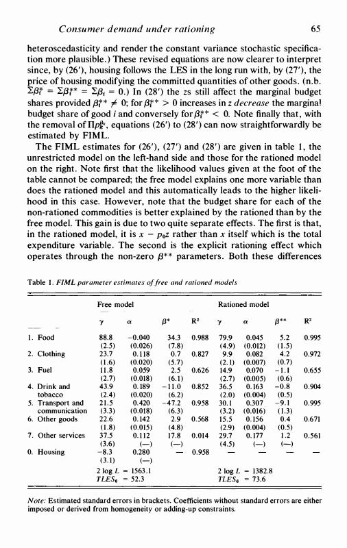
Consumer demand under rationing 65

heteroscedasticity and render the constant variance stochastic specifica­tion more plausible . ) These revised equations are now clearer to interpret since, by (26'), housing follows the LES in the long run with, by (27'), the price of housing modifying the committed quantities of other goods. (n.b. "Lf3f = "Lf3t* = 2.{3; = 0.) In (28') the zs still affect the marginal budget shares provided f3t* I 0; for f3t* > 0 increases in z decrease the marginal budget share of good i and conversely for f3t* < 0. Note finally that , with the removal of llp�\ equations (26') to (28') can now straightforwardly be estimated by FIML.

The FIML estimates for (26'), (27') and (28' ) are given in table 1 , the unrestricted model on the left-hand side and those for the rationed model on the right . Note first that the likelihood values given at the foot of the table cannot be compared; the free model explains one more variable than does the rationed model and this automatically leads to the higher likeli­hood in this case. However, note that the budget share for each of the non-rationed commodities is better explained by the rationed than by the free model. This gain is due to two quite separate effects . The first is that, in the rationed model, it is x - PoZ rather than x itself which is the total expenditure variable . The second is the explicit rationing effect which operates through the non-zero {3** parameters . Both these differences

Table I . F/ML parameter estimates of free and rationed models

Free model Rationed model

'Y a f3* R2 'Y a {3** R2

1 . Food 88.8 -0.040 34.3 0.988 79.9 0.045 5.2 0.995 (2.5) (0.026) (7.8) (4.9) (0.012) ( 1 .5)

2. Clothing 23.7 0. 1 18 0.7 0.827 9.9 0.082 4.2 0.972 ( 1 .6) (0.020) (5.7) (2. l) (0.007) (0.7)

3. Fuel 1 1 .8 0.059 2.5 0.626 14.9 0.070 - l . l 0.655 (2.7) (0.018) (6. l ) (2.7) (0.005) (0.6)

4. Drink and 43.9 0. 189 - 1 1 .0 0.852 36.5 0. 163 -0.8 0.904 tobacco (2.4) (0.020) (6.2) (2.0) (0.004) (0.5)

5. Transport and 2 1 .5 0.420 -47.2 0.958 30. l 0.307 -9. l 0.995 communication (3.3) (0.018) (6.3) (3.2) (0.016) ( l .3)

6. Other goods 22.6 0. 142 2.9 0.568 15.5 0. 156 0.4 0.671 ( 1 .8) (0.015) (4.8) (2.9) (0.004) (0.5)

7 . Other services 37.5 0. 1 12 17.8 0.014 29.7 0. 177 1 .2 0.561 (3.6) (-) (-) (4.5) (-) (-)

0. Housing -8.3 0.280 0.958 (3. l ) (-)

2 log L = 1563 . l 2 log L = 1382.8 TLES6 = 52.3 TLES6 = 73.6

Note: Estimated standard errors in brackets. Coefficients without standard errors are either imposed or derived from homogeneity or adding-up constraints.

66 A . s . D E A T O N

make a contribution. If free and rationed LES models are estimated, i .e. by setting J3f to zero for (27 ') andJ3t* to zero for (28 '), the rationed model fits better to the unrationed commodities. The effect of introducing the J3* and J3** is then assessed by a x2-test on the joint significance of these parameters in each of the models. These tests are the TLES6 figures given in table 1 which, in both cases, indicate the importance of the J3-parameters . For both models, the parameters for food and for transport and communication are highly significant with that for clothing also so in the rationed model. Hence, if we believe the latter, an increase in housing services (e.g. by an unwanted increase in education raised by higher local rates) causes (apart from income effects) a cut in consumption of food and clothing and an increase in the consumption of transport and com­munication.

Although I believe these results to be promising, I must conclude this section with some caveats , both theoretical and econometric. First, although the unrationed model (26') aggregates perfectly over consumers, so justifying an aggregate approach on per capita data, this is not true of the rationed model (28') if the ration levels z vary over households. Sec­ondly, there is a good deal of inconsistency between the two sets of parameter estimates in table 1 . Of course, since each model implies the in­correctness of the other, inconsistencies are to be expected. If the ra­tioned model is true, the explanation of housing in the free model is quite incorrect while the other equations are mis-specified by the omission of z . Conversely, if the free model is correct, the rationed model will suffer from simultaneity bias since z is jointly determined with the other quan­tities . It is thus not clear without a good deal more analysis whether the inconsistencies can be explained by these factors. In any case, the J3* and J3** parameters (n.b. in theory J3** = 1hJ3*) are not all well determined and are rather sensitive to the stochastic specification. They should not therefore be taken too seriously at this stage. Thirdly , and finally , the LES (and even the minor extension embodied in (26') and (27')) is a highly restrictive model which undoubtedly omits or biases important deter­minants of behaviour, see e.g. Deaton ( 1974). Hence, it is not difficult to find essentially spurious correlations by introducing new variables into the model which are correlated with omitted effects. I turn to this in detail in the next section where a much more general model is analysed.

3 A general model for rationed demands

The restrictiveness of the model analysed in the previous section was a consequence of the need to select a functional form for the cost function which permitted an explicit solution of the equations leading to the matched pair of rationed and unrationed demands . If general functional

Consumer demand under rationing 67

forms are assumed for the unrationed cost function, it is rarely possible to solve equation ( 15) for the function �0(u, z, p). For specific examples, so­lutions could be generated numerically and a rationed system of demand functions estimated with knowledge of only the unrestricted cost func­tion. However, in many situations, matched demand functions are unnec­essary and all that is required is a general procedure for producing utility-consistent rationed demand functions . This will be the case, for ex­ample, in the analysis of public goods where we are interested not in how consumers would provide such goods for themselves, but rather in how the public goods levels affect the structure of private consumption. Now, in the unrationed case, the fundamental theorem of duality tells us that, given a cost function with all the correct properties (positive linear homo­geneous, concave , etc .), preferences can always be recovered from it, so that, instead of starting from the specification of a utility function, it is equally valid to start from the cost function. Similarly, given knowledge of its properties, the restricted cost function can be used in exactly the same way.

Recall equation ( 10) and the definition of y(u, z, p) , i .e.

y(u, z , p) = min {p · q; v(z, q) � u} (29) q

where we now allow z to be a vector of ration levels. The function y (u, z , p) is simply the rationed cost function c*(u, p0 , p, z) less the cost of the ra­tion PoZ · Note first that, regarded as a function of u and p, y(u, z, p) has all the conventional properties of a cost function, including the derivative property for the unrationed demands , i .e . ay(u, z, p)/ap; = q;. It thus only remains to categorize the properties with respect to z. The function y(u, z , p) i s a special case of a restricted profit function (see McFadden, 1978), and a full treatment can be found in that reference. For the following dis­cussion, I wish to focus on only two properties, that y(u, z, p) is de­creasing and convex in z .

Both propositions can be established directly from (29). Let z0 be some arbitrary z, with q0 the cost minimizing selection of q given u and z0• For any z1 � z0, v(z1 , if) � v(z0, q0) = u, so that u can be reached or improved upon at q0 for u and z1 • But this is not necessarily the best way of doing so. Hence, y(u, z1 , p) s; y(u, z0, p) for all z1 � z0• The inequality is clearly strict if non-satiation is also assumed. Note that if, in addition, y(u, z , p) is differentiable in z , then, from ( 13)

ay(u, z, p) /:. ( ) az = - !:>O U , Z, p (30)

so that �0(u, z , p) is positive given non-satiation. Convexity of y(u, z , p) in z follows from the convexity of preferences as we now demonstrate. Let

68 A . S . D E A T O N

z1 and z2 be two vectors of rations and let q1 and q2 be the corresponding optimal choices for unrationed goods at utility u and prices p. Hence y(u, z1 , p) = p . q1 and y(u, z2 , p) = p . q2 while, since utility is the same in both situations,

v(q1 , zl) = v(qz, z2) = u

Hence, by the quasi-concavity of v( ) , for 0 :s; A. :s; 1 ,

v(A.q1 + ( 1 - A.)qz, A.z1 + ( 1 - A.)z2) ;:::: u

(3 1)

(32)

Hence, A.q1 + ( 1 - A.)q2 is one way of attaining at least u given A.z1 + ( 1 - A.)z2 and prices p, but not necessarily the cheapest. In other words

so that

y(u, A.z1 + ( 1 _ A.)z2, p) ::; A.p.q1 + ( 1 _ A.)p.qz

y(u, A.z1 + ( 1 - A.)z2, p) :s; A.y(u, z1 , p) + ( 1 - A.)y(u , z2 , p) (33)

which establishes the convexity of the function. Given these results , the analysis of rationed behaviour can proceed

from the specification of a suitable function for y(u , z , p) possessed of the properties discussed above . In Deaton and Muellbauer ( 1980b) a flexible functional form for an unrestricted cost function was proposed which led to the Almost Ideal Demand System (AIDS) in which the budget shares of each commodity are linearly related to the logarithms of prices and price-deflated total expenditure . To define an analogous model which allows for a single ration z, define

log y(u, z, p) = ao + L {ak + '1/kZ} log Pk

1 + 2 L L YZ1 log Pk log P; k j

+ /3ollp�• { u + fJoZ + � 81z2 + � 82uz} (34)

(The extension to a vector of zs is straightforward.) The demand functions can be derived from w1 = a log y/ a log p1 giving budget shares as a propor­tion of total non-rationed expenditure . Hence,

where

(x - PoZ) w, = ai + '1/iZ + L 'Yv log P; + /31 log p j

(35)

1 log P = a0 + L {ak + '1/kZ} log Pk + 2 LL 'YkJ log Pk log P; (36)

k

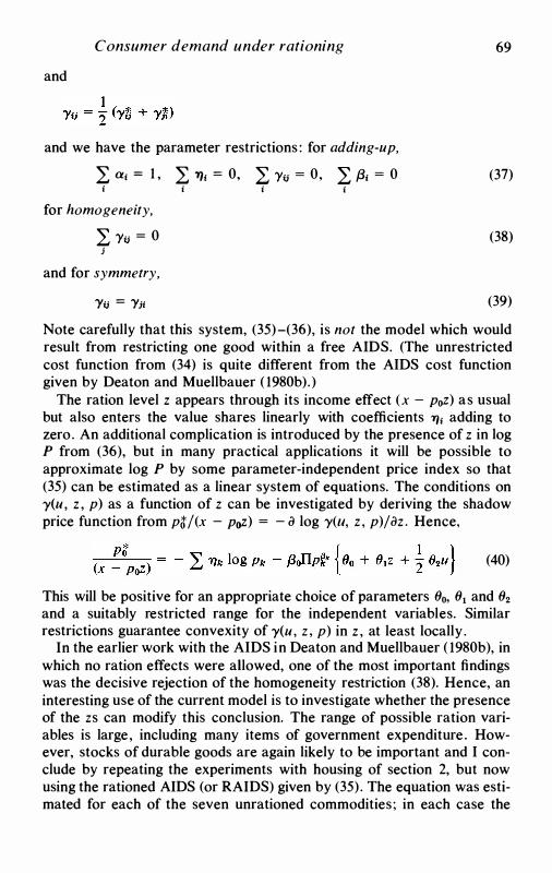
Consumer demand under rationing

and

and we have the parameter restrictions : for adding-up,

L a1 = 1 , L T/1 = o, L yij = o, L /31 = o i i i i

for homogeneity,

L yij = o j

and for symmetry,

Yij = Yit

69

(37)

(38)

(39)

Note carefully that this system, (35)-(36), is not the model which would result from restricting one good within a free AIDS. (The unrestricted cost function from (34) is quite different from the AIDS cost function given by Deaton and Muellbauer ( 1980b).)

The ration level z appears through its income effect (x - PoZ) as usual but also enters the value shares linearly with coefficients T/t adding to zero. An additional complication is introduced by the presence of z in log P from (36), but in many practical applications it will be possible to approximate log P by some parameter-independent price index so that (35) can be estimated as a linear system of equations. The conditions on y(u , z , p) as a function of z can be investigated by deriving the shadow price function from ptf(x - PoZ) = - a log y(u, z , p)/az . Hence,

(40)

This will be positive for an appropriate choice of parameters 80, 81 and 82 and a suitably restricted range for the independent variables. Similar restrictions guarantee convexity of y(u , z , p) in z , at least locally.

In the earlier work with the AIDS in Deaton and Muellbauer ( 1980b), in which no ration effects were allowed, one of the most important findings was the decisive rejection of the homogeneity restriction (38). Hence, an interesting use of the current model is to investigate whether the presence of the zs can modify this conclusion. The range of possible ration vari­ables is large, including many items of government expenditure. How­ever, stocks of durable goods are again likely to be important and I con­clude by repeating the experiments with housing of section 2, but now using the rationed AIDS (or RAIDS) given by (35) . The equation was esti­mated for each of the seven unrationed commodities ; in each case the

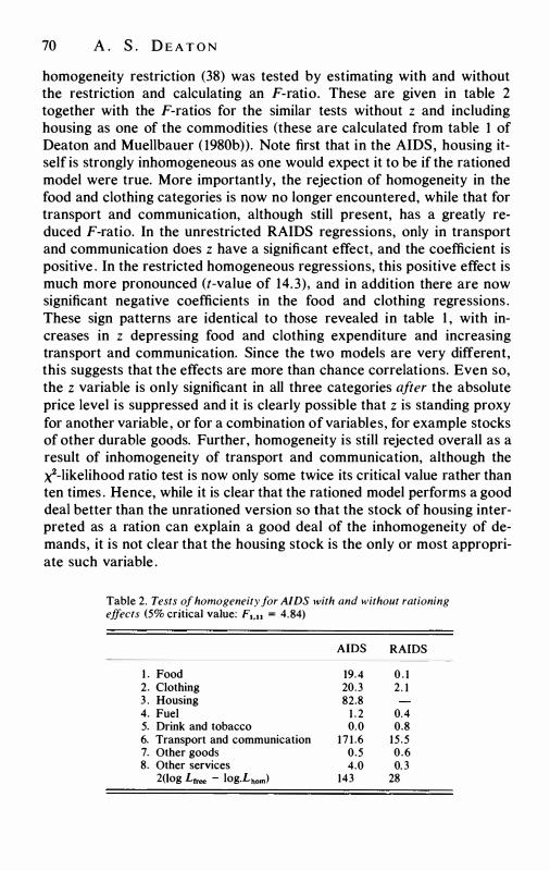
70 A . S . D E A T O N

homogeneity restriction (38) was tested by estimating with and without the restriction and calculating an F-ratio. These are given in table 2 together with the F-ratios for the similar tests without z and including housing as one of the commodities (these are calculated from table 1 of Deaton and Muellbauer ( 1980b)). Note first that in the AIDS, housing it­self is strongly inhomogeneous as one would expect it to be if the rationed model were true. More importantly, the rejection of homogeneity in the food and clothing categories is now no longer encountered, while that for transport and communication, although still present, has a greatly re­duced F-ratio. In the unrestricted RAIDS regressions, only in transport and communication does z have a significant effect, and the coefficient is positive . In the restricted homogeneous regressions, this positive effect is much more pronounced (!-value of 14.3), and in addition there are now significant negative coefficients in the food and clothing regressions . These sign patterns are identical to those revealed in table l , with in­creases in z depressing food and clothing expenditure and increasing transport and communication. Since the two models are very different, this suggests that the effects are more than chance correlations. Even so, the z variable is only significant in all three categories after the absolute price level is suppressed and it is clearly possible that z is standing proxy for another variable , or for a combination of variables, for example stocks of other durable goods. Further, homogeneity is still rejected overall as a result of inhomogeneity of transport and communication, although the x2-likelihood ratio test is now only some twice its critical value rather than ten times . Hence, while it is clear that the rationed model performs a good deal better than the unrationed version so that the stock of housing inter­preted as a ration can explain a good deal of the inhomogeneity of de­mands, it is not clear that the housing stock is the only or most appropri­ate such variable .

Table 2. Tests of homogeneity for AIDS with and without rationing effects (5% critical value: F1,11 = 4.84)

1 . Food 2. Clothing 3 . Housing 4. Fuel 5. Drink and tobacco 6. Transport and communication 7. Other goods 8. Other services

2(1og Lrree - log.Lhom)

AIDS RAIDS

19.4 20.3 82.8

1 . 2 0.0

171 .6 0.5 4.0

143

0 . 1 2. 1

0.4 0.8

15.5 0.6 0. 3

28

Consumer demand under rationing 7 1

4 Conclusions

In this paper, I have discussed the theory of rationed demand functions and presented a method for generating rationed from unrationed de­mands. The technique was applied to an extended version of the linear expenditure system and the resulting model used to investigate the effects of treating the housing stock as a ration level. The empirical results suggested the existence of effects running from an increase in housing to compensating decreases in food and clothing expenditure and compen­sating increases in transport and communication. Finally, a methodology for generating flexible functional forms for rationed demands was pre­sented. This was used to generate an 'almost ideal demand system' with rationing which, when applied to the same data, produced results consist­ent in direction with the first rationed model. Furthermore, the treatment of housing as a ration helped to explain much of the apparent inhomogen­eity in the demand functions. These results suggest that the role of stocks treated as rations is a topic worthy of a good deal more investigation.

Notes

1 I am grateful to John Muellbauer for helpful comments.

References

Barro, R. and Grossman, H. ( 1976), Money, Employment and Inflation, Cam­bridge University Press.

Deaton, A . S. ( 1974), 'A reconsideration of the empirical implications of additive preferences' , Economic Journal, 84, pp. 338-48.

( 1975), Models and Projections of Demand in Post-war Britain, Chapman and Hall, London.

( 1978), 'Specification and testing in applied demand analysis' , Economic Journal, 88, pp. 524-36.

Deaton, A. S. and Muellbauer, J. ( 1980a), Economics and Consumer Behaviour, Cambridge University Press.

( 1980b), 'An almost ideal demand system' , American Economic Review 70, pp. 3 12-26

Deaton, A. S. and Muellbauer, J. ( 198 1) , ' Functional forms for labour supply and commodity demands with and without quantity constraints' , Econometrica, 49, forthcoming.

McFadden, D. ( 1 978), 'Cost, revenue and profit functions' , in Fuss, M. and D. McFadden (eds. ) , Production Economics: a dual approach to theory and ap­plications, North-Holland .

Malinvaud, E. ( 1977), The Theory of Unemployment Reconsidered, Oxford, Basil Blackwell .

Muellbauer, J. ( 198 1 ), ' Linear aggregation in neoclassical labour supply' , Review of Economic Studies, 48, pp. 2 1 -36.

72 A . S . D E A T O N

Muellbauer, J . and Portes , R . ( 1978), 'Macroeconomic models with quantity ra­tioning' , Economic Journal, 88, pp. 788-821 .

Neary, J . P. and Roberts, K . W. S . ( 1980) , 'The theory of household behaviour under rationing' , European Economic Review, 13, pp. 25-42.

Pollak, R. A. ( 1969), 'Conditional demand functions and consumption theory ' , Quarterly Journal of Economics, 83, pp. 70-8.

( 1971) , 'Conditional demand functions and the implications of separable utility' , Southern Economic Journal, 37, pp. 423 -33.

Rothbarth, E. ( 1941) , 'The measurement of change in real income under condi­tions of rationing' , Review of Economic Studie s , 8, pp. 100-7 .

Samuelson, P. A. ( 1947), Foundations of Economic Analysis, Cambridge, Massa­chusetts: Harvard University Press.

Stone, J. R. N. ( 1954), 'Linear expenditure systems and demand analysis: an ap­plication to the pattern of British demand' , Economic Journal, 64, pp. 5 1 1 -27.

Tobin, J. ( 1952), 'A survey of the theory of rationing' , Econometrica , 20, pp. 5 12-53.

Tobin, J. and Houthakker, H. S. ( 195 1 ) , 'The effects of rationing on demand elas­ticities' , Review of Economic Studies, 18, pp. 140-53.

4 The independence transformation: a review and some further

explorations1

H E N R I T H E I L

A N D K E N N E T H LA I T I N E N

1 Introduction

The objective of this chapter is to discuss the relationship between the technique of principal components, first applied to economic data in the pioneering paper by Stone ( 1947), and the analysis of consumer demand.

The purpose of principal component analysis in statistics is to formulate a set of variables that are in some way 'more basic' than the observed variables . Factor analysis has a similar objective. Starting in 1956, Gorman and his associates (Boyle et al. , 1977; Gorman, 1956; 1959; 1976b) applied these statistical techniques to consumer demand in order to assess the consumer's basic wants, while Lancaster ( 1 966, 197 1) and Becker ( 1965) pursued similar goals by extending the economic theory of the consumer rather than using statistical tools. The independence trans­formation, which originated with Theil ( 1967; 1975-76; 1977), Brooks ( 1970), and Laitinen and Theil ( 1978) , is related to both approaches and is in fact 'between' them. The transformation requires no extension of the theory of the utility-maximizing consumer, although it can handle such extensions without difficulty (see the example on leisure in section 2) . At the same time, the transformation has a simple statistical interpretation, viz . , that of a constrained principal component transformation.

To provide adequate motivation, we discuss some examples in section 2. Sections 3 and 4 describe the preference independence transformation and the underlying differential approach to consumption theory. Section 5 gives a brief discussion of similar results in the theory of the firm. A com­parison with principal components follows in section 6, after which the ar­ticle concludes with two sections (7 and 8) on strong and weak separabil­ity. To simplify the exposition, the more complicated mathematics has been put into the appendix. The account which follows is largely exposi­tory, but there are some new results, in particular on the independence

73

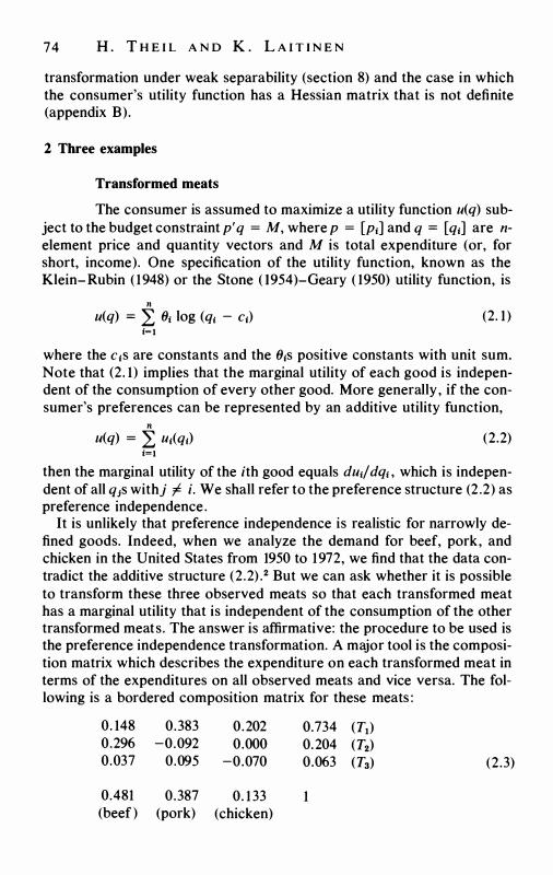
74 H. T H E I L A N D K . L A I T I N E N

transformation under weak separability (section 8) and the case in which the consumer's utility function has a Hessian matrix that is not definite (appendix B).

2 Three examples

Transformed meats

The consumer is assumed to maximize a utility function u(q) sub­ject to the budget constraint p' q = M, where p = [p1] and q = [q1] are n­element price and quantity vectors and M is total expenditure (or, for short, income). One specification of the utility function, known as the Klein-Rubin ( 1948) or the Stone ( 1954)-Geary ( 1950) utility function, is

n u(q) = L 01 log (q1 - c1) (2. 1)

i=l where the c1s are constants and the 01s positive constants with unit sum. Note that (2. 1) implies that the marginal utility of each good is indepen­dent of the consumption of every other good. More generally , if the con­sumer's preferences can be represented by an additive utility function,

n u(q) = L u1(q1) (2.2)

i=l then the marginal utility of the ith good equals duif dqi , which is indepen­dent of all q1s withj I- i. We shall refer to the preference structure (2 .2) as preference independence.

It is unlikely that preference independence is realistic for narrowly de­fined goods. Indeed, when we analyze the demand for beef, pork, and chicken in the United States from 1950 to 1972, we find that the data con­tradict the additive structure (2.2) .2 But we can ask whether it is possible to transform these three observed meats so that each transformed meat has a marginal utility that is independent of the consumption of the other transformed meats. The answer is affirmative: the procedure to be used is the preference independence transformation. A major tool is the composi­tion matrix which describes the expenditure on each transformed meat in terms of the expenditures on all observed meats and vice versa. The fol­lowing is a bordered composition matrix for these meats :

0. 148 0.383 0.202 0.734 (T1) 0.296 -0.092 0.000 0.204 (T2) 0.037 0.095 -0.070 0.063 (Ta) (2.3)

0.481 0.387 0. 1 33 1 (beef) (pork) (chicken)

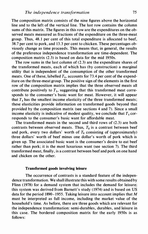
The independence transformation 75

The composition matrix consists of the nine figures above the horizontal line and to the left of the vertical line. The last row contains the column sums of this matrix . The figures in this row are the expenditures on the ob­served meats measured as fractions of the expenditure on the three-meat group. Thus, 48. 1 per cent of this total expenditure is allocated to beef, 38.7 per cent to pork, and 13 .3 per cent to chicken. These percentages ob­viously change as time proceeds. This means that, in general , the results of the preference independence transformation are time-dependent. The composition matrix (2 .3) is based on data for the mid 1950s.

The row sums in the last column of (2.3) are the expenditure shares of the transformed meats , each of which has (by construction) a marginal utility that is independent of the consumption of the other transformed meats. One of these, labelled Tb accounts for 73.4 per cent of the expend­iture on the three-meat group. The positive sign of the elements in the first row of the composition matrix implies that the three observed meats all contribute positively to Tb suggesting that this transformed meat corre­sponds to the consumer' s basic want for meat. However, it will appear that T1 has the smallest income elasticity of the three transformed meats ; these elasticities provide information on transformed goods beyond that provided by the composition matrix (see sections 4 and 7). Since a small income elasticity is indicative of modest quality, we conclude that T1 cor­responds to the consumer's basic want for affordable meat.

The transformed meats in the second and third rows of (2 .3) are both contrasts between observed meats . Thus, T2 is a contrast between beef and pork, every two dollars' worth of T2 consisting of (approximately) three dollars' worth of beef minus one dollar's worth of pork which is given up. The associated basic want is the consumer's desire to eat beef rather than pork ; it is the most luxurious want (see section 7). The third transformed meat, finally , is a contrast between beef and pork on one hand and chicken on the other.

Transformed goods involving leisure

The occurrence of contrasts is a standard feature of the indepen­dence transformation. We shall illustrate this with some results obtained by Flinn ( 1978) for a demand system that includes the demand for leisure; this system was derived from Barnett's study ( 1974) and is based on US data for the period 1890- 1955. Taking leisure into account implies that M must be interpreted as full income, including the market value of the household's time. As before, there are three goods which are relevant for the independence transformation: semi-durables, durables , and leisure in this case. The bordered composition matrix for the early 1950s is as follows:

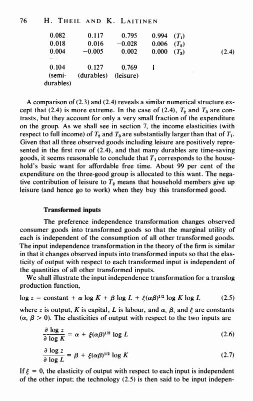
76 H . T H E I L A N D K . L A I T I N E N

0.082 0. 1 17 0.795 0.994 (Ti) 0.018 0.016 -0.028 0.006 (T2) 0.004 -0.005 0.002 0.000 (Ta) (2.4)

0. 104 0. 127 0.769 (semi- (durables) (leisure)

durables)

A comparison of (2.3) and (2.4) reveals a similar numerical structure ex­cept that (2.4) is more extreme. In the case of (2.4) , T2 and Ta are con­trasts , but they account for only a very small fraction of the expenditure on the group. As we shall see in section 7, the income elasticities (with respect to full income) of T2 and Ta are substantially larger than that of Ti. Given that all three observed goods including leisure are positively repre­sented in the first row of (2.4) , and that many durables are time-saving goods, it seems reasonable to conclude that Ti corresponds to the house­hold's basic want for affordable free time. About 99 per cent of the expenditure on the three-good group is allocated to this want . The nega­tive contribution of leisure to T2 means that household members give up leisure (and hence go to work) when they buy this transformed good.

Transformed inputs

The preference independence transformation changes observed consumer goods into transformed goods so that the marginal utility of each is independent of the consumption of all other transformed goods. The input independence transformation in the theory of the firm is similar in that it changes observed inputs into transformed inputs so that the elas­ticity of output with respect to each transformed input is independent of the quantities of all other transformed inputs.

We shall illustrate the input independence transformation for a translog production function,

log z = constant + a log K + {3 log L + g(a{3)i12 log K log L (2.5)

where z is output, K is capital , L is labour, and a, {3, and g are constants (a, {3 > 0). The elasticities of output with respect to the two inputs are

a log z --- = a + g(a{3)i12 log L a log K

a log z --- = {3 + g(a{3)112 log K a log L

(2.6)

(2.7)

If g = 0, the elasticity of output with respect to each input is independent of the other input; the technology (2.5) is then said to be input indepen-

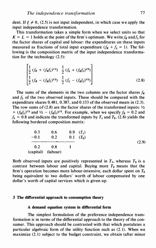
The independence transformation 77

dent. If � I- 0, (2.5) is not input independent, in which case we apply the input independence transformation.

This transformation takes a simple form when we select units so that K = L = 1 holds at the point of the firm's optimum. We writefK andfL for the factor shares of capital and labour: the expenditures on these inputs measured as fractions of total input expenditure <fK + fL = 1 ) . The fol­lowing is the composition matrix of the input independence transforma­tion for the technology (2.5): [t lfx + lfxAl"') i lf, + lfJd")]

2 (fK - (f JL)112) � (fL - (f JL)112) (2.8)

The sums of the elements in the two columns are the factor shares fK and fL of the two observed inputs. These should be compared with the expenditure shares 0.48 1 , 0.387, and 0. 133 of the observed meats in (2.3) . The row sums of (2.8) are the factor shares of the transformed inputs: \12 + (fJL)112 and \12 - (fJL)112. For example, when we specify A = 0.2 and fL = 0.8 and indicate the transformed inputs by T1 and T2, (2.8) yields the following bordered composition matrix :

0.3 0.6 0.9 (T1) -0. l 0.2 0. 1 (T2)

(2.9) 0.2 0.8

(capital) (labour)

Both observed inputs are positively represented in Ti. whereas T2 is a contrast between labour and capital. Buying more T2 means that the firm's operation becomes more labour-intensive, each dollar spent on T2 being equivalent to two dollars' worth of labour compensated by one dollar's worth of capital services which is given up.

3 The differential approach to consumption theory

A demand equation system in differential form

The simplest formulation of the preference independence trans­formation is in terms of the differential approach to the theory of the con­sumer. This approach should be contrasted with that which postulates a particular algebraic form of the utility function such as (2. 1) . When we maximize (2. 1 ) subject to the budget constraint, we obtain (after minor

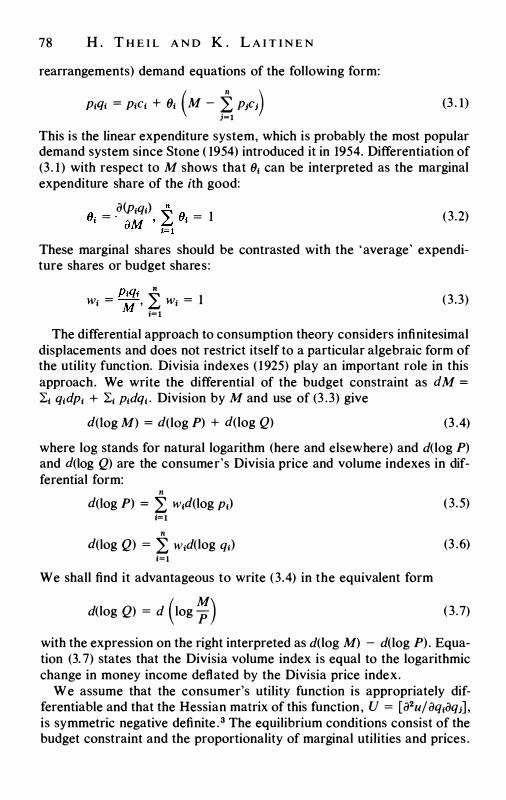
78 H . T H E I L A N D K . L A I T I N E N

rearrangements) demand equations of the following form:

P1q1 = P1C1 + 81 ( M - � P;c;) (3 . 1)

This is the linear expenditure system, which is probably the most popular demand system since Stone ( 1954) introduced it in 1954. Differentiation of (3 . 1 ) with respect to M shows that 81 can be interpreted as the marginal expenditure share of the ith good:

" · = a(p1q1) � ,. = 1 u, aM , � u1 •=!

(3.2)

These marginal shares should be contrasted with the 'average' expendi­ture shares or budget shares:

W1 = P::i ' i W1 = 1 i=I

(3.3)

The differential approach to consumption theory considers infinitesimal displacements and does not restrict itself to a particular algebraic form of the utility function. Divisia indexes ( 1925) play an important role in this approach. We write the differential of the budget constraint as dM = L1 q1dP1 + L1 p1dq1 . Division by M and use of (3 .3) give

d(log M) = d(log P) + d(log Q) (3 .4)

where log stands for natural logarithm (here and elsewhere) and d(log P) and d(log Q) are the consumer's Divisia price and volume indexes in dif­ferential form: n

d(log P) = L w1d(log P1) (3.5) i=I n

d(log Q) = L w1d(log qi) (3 .6) i=!

We shall find it advantageous to write (3.4) in the equivalent form

d(log Q) = d (log �) (3 .7)

with the expression on the right interpreted as d(log M) - d(log P). Equa­tion (3. 7) states that the Divisia volume index is equal to the logarithmic change in money income deflated by the Divisia price index.

We assume that the consumer's utility function is appropriately dif­ferentiable and that the Hessian matrix of this function, U = [ a2 u / aq1aq;] , is symmetric negative definite . 3 The equilibrium conditions consist of the budget constraint and the proportionality of marginal utilities and prices .

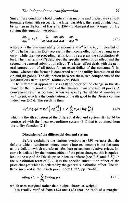
The independence transformation 79

Since these conditions hold identically in income and prices, we can dif­ferentiate them with respect to the latter variables, the result of which can be written in the form of Barten's ( 1964) fundamental matrix equation. By solving this equation we obtain

iJq; .. >.. iJq; iJq1 iJq; iJp1

= >..uu - iJA./iJM iJM iJM - iJM q1 (3.8)

where >.. is the marginal utility of income and ui.i is the (i, 1)th element of u-1 • The last term in (3 .8) represents the income effect of the change in p1 on qi, while the two preceding terms jointly represent the substitution ef­fect. The firm term (A.ui.i) describes the specific substitution effect and the second the general substitution effect. The latter effect deals with the gen­eral competition of all goods for an extra dollar of the consumer's in­come, whereas the former is concerned with the utility interaction of the ith and jth goods. The distinction between these two components of the substitution effect is from Houthakker ( 1960).

The differential approach uses (3 .8) to describe the change in the de­mand for the ith good in terms of the changes in income and all prices. A convenient result is obtained when we specify the left-hand variable as w;d(log q;), which is the contribution of the ith good to the Divisia volume index [see (3 .6)]. The result is then

w;d(log q;) = 81d (log �) + cf> � 8ud (log ;�) (3.9)

which is the ith equation of the differential demand system. It should be contrasted with the linear expenditure system (3 . 1 ) that is obtained from the utility function (2 . 1 ) .

Discussion of the differential demand system

Before explaining the various symbols in (3.9) we note that the deflator which transforms money income into real income is not the same as the deflator which transforms absolute prices into relative prices . In­come is deflated by the income effect of the price changes; this is equiva­lent to the use of the Divisia price index as deflator [see (3.5) and (3.7)]. In the substitution term of (3.9) it is the specific substitution effect of the price changes which is deflated by the general substitution effect. The de­flator involved is the Frisch price index ( 1932, pp. 74-82) ,

n d(log P') = L 8;d(log p;) (3 . 10)

i=l

which uses marginal rather than budget shares as weights . It is readily verified from (3.2) and (3.3) that the ratio of a marginal

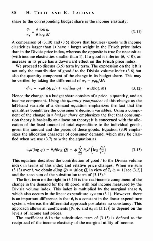
80 H . T H E I L A N D K . L A I T I N E N

share to the corresponding budget share is the income elasticity :

81 a log q1 wi a log M

(3 . 1 1)

A comparison of (3 . 10) and (3.5) shows that luxuries (goods with income elasticities larger than 1) have a larger weight in the Frisch price index than in the Divisia price index, whereas the opposite is true for necessities (with income elasticities smaller than 1) . If a good is inferior (81 < 0), an increase in its price has a downward effect on the Frisch price index.

We proceed to discuss (3 .9) term by term. The expression on the left is not only the contribution of good i to the Divisia volume index (3 .6) but also the quantity component of the change in its budget share . This may be verified by taking the differential of wi = Piqi/ M:

(3 . 12)

Hence the change in a budget share consists of a price, a quantity, and an income component. Using the quantity component of this change as the left-hand variable of a demand equation emphasizes the fact that the quantities bought are the consumer' s decision variables. Using a compo­nent of the change in a budget share emphasizes the fact that consump­tion theory is basically an allocation theory ; it is concerned with the allo­cation of the fixed amount of total expenditure to the individual goods , given this amount and the prices of these goods. Equation (3.9) empha­sizes the allocation character of consumer demand, which may be clari­fied when we use (3. 7) to write the equation as

w1d(log q1) = 81d(log Q) + <f> � (Jiid (log ;�) (3 . 1 3)

This equation describes the contribution of good i to the Divisia volume index in terms of this index and relative price changes . When we sum (3. 13) over i, we obtain d(log Q) = d(log Q) in view of L; (Ji = 1 [see (3 .2)] and the zero sum of the substitution term of (3. 13) . 4

The first term on the right in (3. 1 3) is the real-income component of the change in the demand for the ith good, with real income measured by the Divisia volume index. This index is multiplied by the marginal share 81 which also occurs in the linear expenditure system (3 . 1 ) . However, there is an important difference in that 81 is a constant in the linear expenditure system, whereas the differential approach postulates no constancy . This approach allows all coefficients [8;, <f>, and (}ii in (3 . 13)] to depend on the levels of income and prices .

The coefficient <f> in the substitution term of (3 . 13) is defined as the reciprocal of the income elasticity of the marginal utility of income:

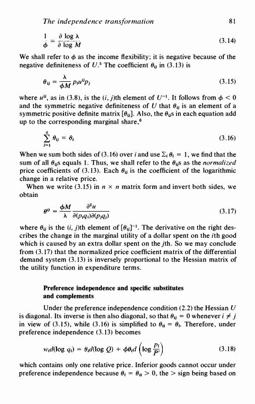
The independence transformation

1 a log A. <f> a log M

8 1

(3 . 14)

We shall refer to <f> as the income flexibility ; it is negative because of the negative definiteness of U.5 The coefficient Ou in (3 . 1 3) is

A. . . Ou = <f>M Piuvpj (3 . 15)

where uu, as in (3.8), is the (i, j)th element of u-1 • It follows from <f> < 0 and the symmetric negative definiteness of U that Ou is an element of a symmetric positive definite matrix [Ou] . Also, the Ous in each equation add up to the corresponding marginal share,6

(3 . 16) j=l

When we sum both sides of (3 . 16) over i and use Li (Ji = 1 , we find that the sum of all Ous equals 1 . Thus, we shall refer to the Ous as the normalized price coefficients of (3 . 13). Each Ou is the coefficient of the logarithmic change in a relative price.

When we write (3. 15) in n x n matrix form and invert both sides, we obtain

.. <PM a2u (J1J = - -----

A. a(piqi)a(pjqj) (3 . 17)

where Ou is the (i, j)th element of [Ou]-1 • The derivative on the right des­cribes the change in the marginal utility of a dollar spent on the ith good which is caused by an extra dollar spent on the jth. So we may conclude from (3. 17) that the normalized price coefficient matrix of the differential demand system (3 . 13) is inversely proportional to the Hessian matrix of the utility function in expenditure terms.

Preference independence and specific substitutes and complements

Under the preference independence condition (2.2) the Hessian U is diagonal . Its inverse is then also diagonal , so that Ou = 0 whenever i I= j in view of (3 . 1 5) , while (3 . 16) is simplified to Ou = (Ji· Therefore, under preference independence (3. 13) becomes

(3 . 1 8)

which contains only one relative price . Inferior goods cannot occur under preference independence because (Ji = Ou > 0, the > sign being based on

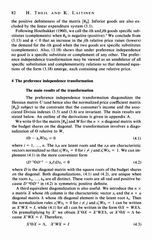
82 H . T H E I L A N D K . L A I T I N E N

the positive definiteness of the matrix [8(i] . Inferior goods are also ex­cluded by the linear expenditure system (3 . 1 ) .

Following Houthakker ( 1960) , we call the ith andjth goods specific sub­stitutes (complements) when 8(i is negative (positive). 7 We conclude from (3 . 13) and 4> < 0 that an increase in the jth relative price raises (lowers) the demand for the ith good when the two goods are specific substitutes (complements). Also, (3. 18) shows that under preference independence no good is a specific substitute or complement of any other. The prefer­ence independence transformation may be viewed as an annihilator of all specific substitution and complementarity relations so that demand equa­tions of the form (3. 18) emerge, each containing one relative price.

4 The preference independence transformation

The main results of the transformation

The preference independence transformation diagonalizes the Hessian matrix U (and hence also the normalized price coefficient matrix [8(i]) subject to the constraint that the consumer's income and the asso­ciated Divisia indexes (3 .5) and (3 .6) are invariant. The main results are stated below. An outline of the derivations is given in appendix A.

We write e for the matrix [8(i] and W for the n x n diagonal matrix with the budget shares on the diagonal . The transformation involves a diago­nalization of e relative to W,

(e - A;W)x; = o (4. 1 )

where i = 1 , . . . , n . The A;S are latent roots and the x;s are characteristic vectors normalized so that xi Wx; = 0 for i I- j and xi Wx; = 1 . We can im­plement (4. 1 ) in the more convenient form

(4.2)

where D is the diagonal matrix with the square roots of the budget shares on the diagonal . Both diagonalizations , (4. 1 ) and (4.2) , are unique when the roots Ai. . . . , An are all distinct. These roots are all real and positive be­cause v-1ev-1 in (4.2) is symmetric positive definite.

A third equivalent diagonalization is also useful . We introduce the n x n matrix X whose ith column is the characteristic vector x; and the n x n diagonal matrix A whose ith diagonal element is the latent root A;. Then the normalization rules xi Wx; = 0 for i I- j and xi Wx; = 1 can be written as X' WX = I, while (4. 1 ) for all i can be written in the form ex = WXA. On premultiplying by X' we obtain X'eX = X' WXA, or X'9X = A be­cause X' WX = I. Therefore,

X'ex = A, X' WX = I (4.3)

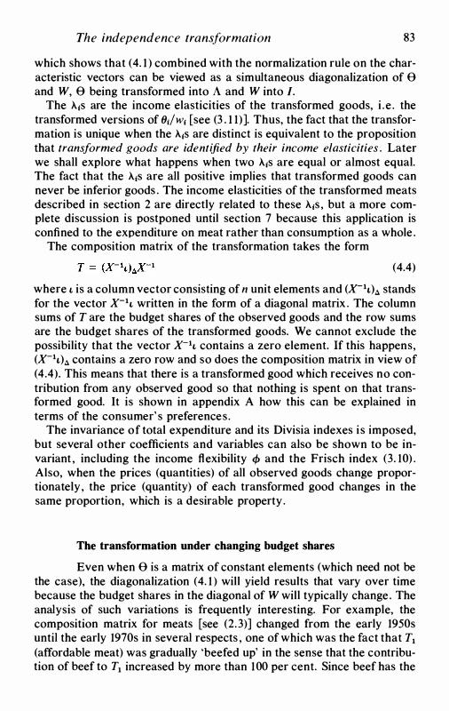
The independence transformation 83

which shows that (4. 1 ) combined with the normalization rule on the char­acteristic vectors can be viewed as a simultaneous diagonalization of e and W, 0 being transformed into A and W into I.

The A.1s are the income elasticities of the transformed goods, i .e . the transformed versions of (Ji/ w1 [see (3 . 1 1) ]. Thus, the fact that the transfor­mation is unique when the A.1s are distinct is equivalent to the proposition that transformed goods are identified by their income elasticities . Later we shall explore what happens when two A.1s are equal or almost equal. The fact that the A.1s are all positive implies that transformed goods can never be inferior goods . The income elasticities of the transformed meats described in section 2 are directly related to these A.1s , but a more com­plete discussion is postponed until section 7 because this application is confined to the expenditure on meat rather than consumption as a whole .

The composition matrix of the transformation takes the form

(4.4)

where t is a column vector consisting of n unit elements and (X-it)<l stands for the vector x-it written in the form of a diagonal matrix . The column sums of T are the budget shares of the observed goods and the row sums are the budget shares of the transformed goods. We cannot exclude the possibility that the vector x-it contains a zero element. If this happens, (X-it)<l contains a zero row and so does the composition matrix in view of (4.4). This means that there is a transformed good which receives no con­tribution from any observed good so that nothing is spent on that trans­formed good. It is shown in appendix A how this can be explained in terms of the consumer' s preferences.

The invariance of total expenditure and its Divisia indexes is imposed, but several other coefficients and variables can also be shown to be in­variant , including the income flexibility </> and the Frisch index (3. 10) . Also, when the prices (quantities) of all observed goods change propor­tionately, the price (quantity) of each transformed good changes in the same proportion, which is a desirable property .

The transformation under changing budget shares

Even when e is a matrix of constant elements (which need not be the case), the diagonalization (4. 1 ) will yield results that vary over time because the budget shares in the diagonal of W will typically change. The analysis of such variations is frequently interesting. For example, the composition matrix for meats [see (2.3)] changed from the early 1950s until the early 1970s in several respects , one of which was the fact that Ti (affordable meat) was gradually 'beefed up' in the sense that the contribu­tion of beef to Ti increased by more than 100 per cent. Since beef has the

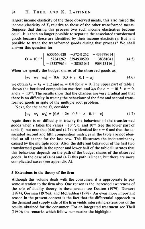
84 H . T H E I L A N D K . L A I T I N E N

largest income elasticity of the three observed meats , this also raised the income elasticity of T1 relative to those of the other transformed meats . Suppose that during this process two such income elasticities become equal . It is then no longer possible to separate the associated transformed goods because these are identified by their income elasticities. But is it possible to trace the transformed goods during that process? We shall answer this question for [ 65536601 28 -57241 262 - 433379614]

e = 10-10 - 57241262 3594930590 - 38381041 - 4333796 14 - 3838 104 1 9094 13 1 16

When we specify the budget shares of the observed goods as

[w1 W2 w3] = [0.6 0.3 + e 0. 1 - e]

(4.5)

(4.6)

we obtain A.1 = A.2 = 1 .2 and A.3 = 0.8 for e = 0. The upper part of table 1 shows the bordered composition matrices and A.;s for e = - 10-s, e = 0, and e = 10-5• The results show that the changes are very gradual and that there is no difficulty in tracing the behaviour of the first and second trans­formed goods in spite of the multiple root problem.

Next, for the same e, consider

[w1 w2 w3] = [0.6 + 2e 0.3 - e 0. 1 - e] (4.7)

Again there is no difficulty in tracing the behaviour of the transformed goods when e takes the values - 10-s, 0, and 10-s (see the lower part of table 1) , but note that (4.6) and (4.7) are identical for e = 0 and that the as­sociated second and fifth composition matrices in the table are not iden­tical at all except for the last row. This illustrates the indeterminancy caused by the multiple roots. Also, the different behaviour of the first two transformed goods in the upper and lower half of the table illustrates that this behaviour depends on the path of the budget shares of the observed goods. In the case of (4.6) and (4.7) this path is linear, but there are more complicated cases (see appendix A) .

5 Extensions to the theory of the firm

Although this volume deals with the consumer, it is appropriate to pay some attention to the firm also. One reason is the increased awareness of the role of duality theory in these areas ; see Deaton ( 1979), Diewert ( 1974), Gorman ( 1976a) , and McFadden ( 1 978). An even more important reason in the present context is the fact that the differential approach to the demand and supply side of the firm yields interesting extensions of the results obtained for the consumer. For an integrated treatment see Theil ( 1980); the remarks which follow summarize the highlights .

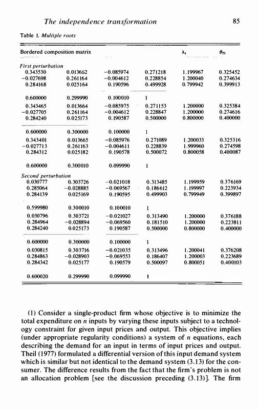
The independence transformation 85

Table I. Multiple roots

Bordered composition matrix A., 9Ti

First perturbation 0.343530 0.013662 -0.085974 0.271218 1 . 199967 0.325452

-0.027698 0.261 164 -0.004612 0.228854 l .200040 0.274634 0.284168 0.025 164 0. 190596 0.499928 0.799942 0.399913

0.600000 0.299990 0. 100010 1

0.343465 0.013664 -0.085975 0.27 1 1 53 l .200000 0.325384 -0.027705 0.261 164 -0.004612 0.228847 1 .200000 0.274616

0.284240 0.025173 0. 190587 0.500000 0.800000 0.400000

0.600000 0.300000 0. 100000

0.343401 0.013665 -0.085976 0.271089 1 .200033 0.3253 16 -0.02771 3 0.261 163 -0.00461 1 0.228839 1 .999960 0.274598

0.2843 12 0.025 182 0. 190578 0.500072 0.800058 0.400087

0.600000 0.300010 0.099990

Second perturbation 0.030777 0.303726 -0.021018 0.313485 1 . 199959 0.376169 0.285064 -0.028885 -0.069567 0. 1 86612 1 . 199997 0.223934 0.284139 0.025 169 0. 190595 0.499903 0.799949 0.399897

0.599980 0.300010 0. 100010

0.030796 0.303721 -0.021027 0.313490 1 .200000 0.376188 0.284964 -0.028894 -0.069560 0. 18 15 10 l . 200000 0.22381 1 0.284240 0.025 173 0 . 190587 0.500000 0.800000 0.400000

0.600000 0.300000 0. 100000

0.030815 0.303716 -0.021035 0.3 13496 1 .200041 0.376208 0.284863 -0.028903 -0.069553 0. 186407 1 .200003 0.223689 0.284342 0.025177 0. 190579 0.500097 0.800051 0.400103

0.600020 0.299990 0.099990

( 1 ) Consider a single-product firm whose objective is to minimize the total expenditure on n inputs by varying these inputs subject to a technol­ogy constraint for given input prices and output. This objective implies (under appropriate regularity conditions) a system of n equations, each describing the demand for an input in terms of input prices and output. Theil ( 1977) formulated a differential version of this input demand system which is similar but not identical to the demand system (3 . 1 3) for the con­sumer. The difference results from the fact that the firm's problem is not an allocation problem [see the discussion preceding (3 . 13) ]. The firm

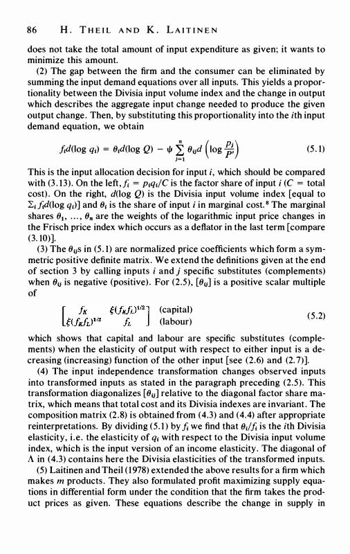
86 H . T H E I L A N D K . L A I T I N E N

does not take the total amount of input expenditure as given; it wants to minimize this amount.

(2) The gap between the firm and the consumer can be eliminated by summing the input demand equations over all inputs. This yields a propor­tionality between the Divisia input volume index and the change in output which describes the aggregate input change needed to produce the given output change. Then, by substituting this proportionality into the ith input demand equation, we obtain

.fid(log q1) = 91d(log Q) - tjJ � 9iJd (log f;,) (5 . 1)

This is the input allocation decision for input i, which should be compared with (3 . 13). On the left, .fi = p1q1/C is the factor share of input i (C = total cost) . On the right, d(log Q) is the Divisia input volume index [equal to L1 .fid(log q1)] and 91 is the share of input i in marginal cost. 8 The marginal shares 91 , • • • , On are the weights of the logarithmic input price changes in the Frisch price index which occurs as a deflator in the last term [compare (3. 10)].

(3) The 9iJs in (5 . 1) are normalized price coefficients which form a sym­metric positive definite matrix . We extend the definitions given at the end of section 3 by calling inputs i and j specific substitutes (complements) when (JiJ is negative (positive) . For (2.5), [9v] is a positive scalar multiple of

(capital) (labour)

(5.2)

which shows that capital and labour are specific substitutes (comple­ments) when the elasticity of output with respect to either input is a de­creasing (increasing) function of the other input [see (2.6) and (2. 7)].

(4) The input independence transformation changes observed inputs into transformed inputs as stated in the paragraph preceding (2.5). This transformation diagonalizes [OiJ] relative to the diagonal factor share ma­trix, which means that total cost and its Divisia indexes are invariant . The composition matrix (2 .8) is obtained from (4.3) and (4.4) after appropriate reinterpretations. By dividing (5. 1 ) by fi we find that 9i/fi is the ith Divisia elasticity, i .e . the elasticity of q1 with respect to the Divisia input volume index, which is the input version of an income elasticity. The diagonal of A in (4.3) contains here the Divisia elasticities of the transformed inputs.

(5) Laitinen and Theil ( 1978) extended the above results for a firm which makes m products . They also formulated profit maximizing supply equa­tions in differential form under the condition that the firm takes the prod­uct prices as given. These equations describe the change in supply in

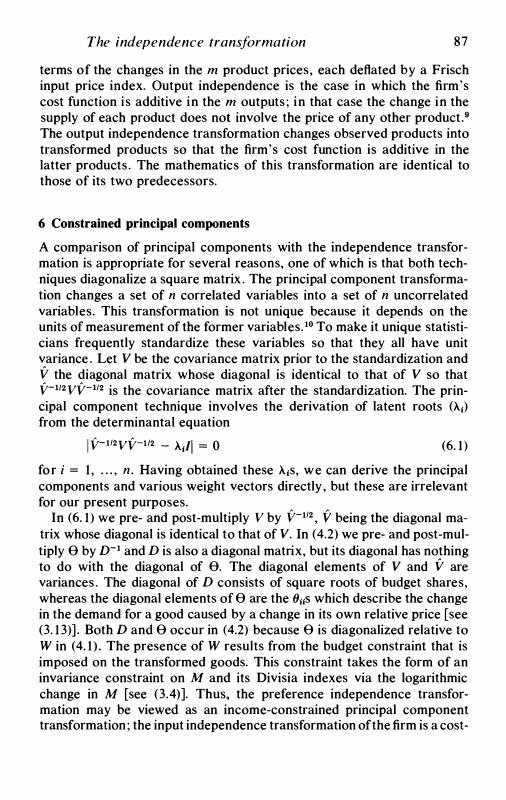
The independence transformation 87

terms of the changes in the m product prices, each deflated by a Frisch input price index. Output independence is the case in which the firm's cost function is additive in the m outputs ; in that case the change in the supply of each product does not involve the price of any other product.9 The output independence transformation changes observed products into transformed products so that the firm's cost function is additive in the latter products . The mathematics of this transformation are identical to those of its two predecessors.

6 Constrained principal components

A comparison of principal components with the independence transfor­mation is appropriate for several reasons, one of which is that both tech­niques diagonalize a square matrix . The principal component transforma­tion changes a set of n correlated variables into a set of n uncorrelated variables. This transformation is not unique because it depends on the units of measurement of the former variables. 10 To make it unique statisti­cians frequently standardize these variables so that they all have unit variance . Let V be the covariance matrix prior to the standardization and V the diagonal matrix whose diagonal is identical to that of V so that v-112vv-112 is the covariance matrix after the standardization. The prin­cipal component technique involves the derivation of latent roots (Ai) from the determinantal equation

i v-112vv-112 - A1II = o (6. 1 )

for i = 1 , . . . , n . Having obtained these A1s, we can derive the principal components and various weight vectors directly , but these are irrelevant for our present purposes.

In (6. 1 ) we pre- and post-multiply v by v-112 ' v being the diagonal ma­trix whose diagonal is identical to that of V. In (4.2) we pre- and post-mul­tiply e by D-1 and D is also a diagonal matrix, but its diagonal has nothing to do with the diagonal of 8. The diagonal elements of V and V are variances . The diagonal of D consists of square roots of budget shares, whereas the diagonal elements of e are the (Jiis which describe the change in the demand for a good caused by a change in its own relative price [see (3. 1 3)] . Both D and e occur in (4.2) because e is diagonalized relative to W in (4. 1 ) . The presence of W results from the budget constraint that is imposed on the transformed goods. This constraint takes the form of an invariance constraint on M and its Divisia indexes via the logarithmic change in M [see (3.4)]. Thus, the preference independence transfor­mation may be viewed as an income-constrained principal component transformation; the input independence transformation of the firm is a cost-

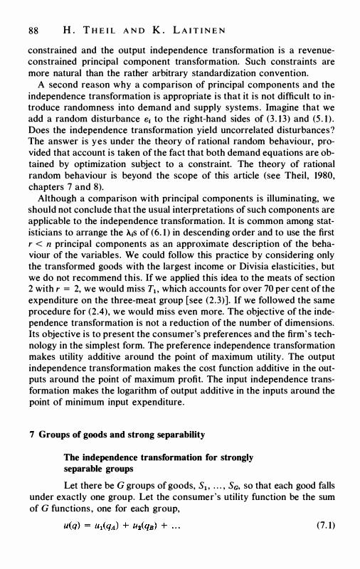
88 H . T H E I L A N D K . L A I T I N E N

constrained and the output independence transformation is a revenue­constrained principal component transformation. Such constraints are more natural than the rather arbitrary standardization convention.

A second reason why a comparison of principal components and the independence transformation is appropriate is that it is not difficult to in­troduce randomness into demand and supply systems. Imagine that we add a random disturbance ei to the right-hand sides of (3 . 13) and (5 . 1 ) . Does the independence transformation yield uncorrelated disturbances? The answer is yes under the theory of rational random behaviour, pro­vided that account is taken of the fact that both demand equations are ob­tained by optimization subject to a constraint. The theory of rational random behaviour is beyond the scope of this article (see Theil, 1980, chapters 7 and 8).

Although a comparison with principal components is illuminating, we should not conclude that the usual interpretations of such components are applicable to the independence transformation. It is common among stat­isticians to arrange the �1s of (6. 1 ) in descending order and to use the first r < n principal components as an approximate description of the beha­viour of the variables. We could follow this practice by considering only the transformed goods with the largest income or Divisia elasticities , but we do not recommend this. If we applied this idea to the meats of section 2 with r = 2, we would miss Ti . which accounts for over 70 per cent of the expenditure on the three-meat group [see (2.3)]. If we followed the same procedure for (2.4), we would miss even more. The objective of the inde­pendence transformation is not a reduction of the number of dimensions. Its objective is to present the consumer's preferences and the firm's tech­nology in the simplest form. The preference independence transformation makes utility additive around the point of maximum utility. The output independence transformation makes the cost function additive in the out­puts around the point of maximum profit. The input independence trans­formation makes the logarithm of output additive in the inputs around the point of minimum input expenditure.

7 Groups of goods and strong separability

The independence transformation for strongly separable groups

Let there be G groups of goods, Si . . . . , Sa, so that each good falls under exactly one group. Let the consumer's utility function be the sum of G functions, one for each group,

(7. 1)

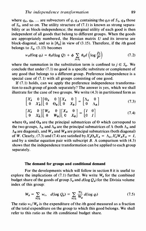
The independence transformation 89

where qA, qB, . . . are subvectors of q, qA containing the q1s of S., qB those of S2, and so on. The utility structure of (7 . 1 ) is known as strong separa­bility or as block-independence; the marginal utility of each good is then independent of all goods that belong to different groups. When the goods are appropriately numbered, the Hessian matrix U and its inverse are block-diagonal , and so is (80] in view of (3 . 15). Therefore, if the ith good belongs to Su, (3 . 13) becomes

w1d(log q;) = 81d(log Q) + <f> .L 8ud (log ;, ) (7 .2) JESu

where the summation in the substitution term is confined to j E Su . We conclude that under (7. 1 ) no good is a specific substitute or complement of any good that belongs to a different group. Preference independence is a special case of (7 . 1) with all groups consisting of one good.

If (7. 1 ) holds, can we apply the preference independence transforma­tion to each group of goods separately? The answer is yes, which we shall illustrate for the case of two groups. We write (4.3) in partitioned form as

[Xo.4 0 ] [eA 0 ] [XA 0 ] [AA 0 ]

x;, o eB o xB =

o AB (7.3)

(7.4)

Where €)A and t)B are the principal SUbmatriCeS Of €) Which COITeSpond to the two groups, AA and AB are the principal submatrices of A (both AA and AB are diagonal), and WA and WB are principal submatrices (both diagonal) of W. Clearly, (7.3) and (7.4) are satisfied by X.40AXA = AA, X.4 WAXA = I, and by a similar equation pair with subscript B. A comparison with (4.3) shows that the independence transformation can be applied to each group separately.

The demand for groups and conditional demand

For the developments which will follow in section 8 it is useful to explore the implications of (7. 1 ) further. We write Wu for the combined budget share of the goods of group Su and d(log Qu) for the Divisia volume index of this group:

(7.5)

The ratio wi/Wu is the expenditure of the ith good measured as a fraction of the total expenditure on the group to which this good belongs. We shall refer to this ratio as the ith conditional budget share.

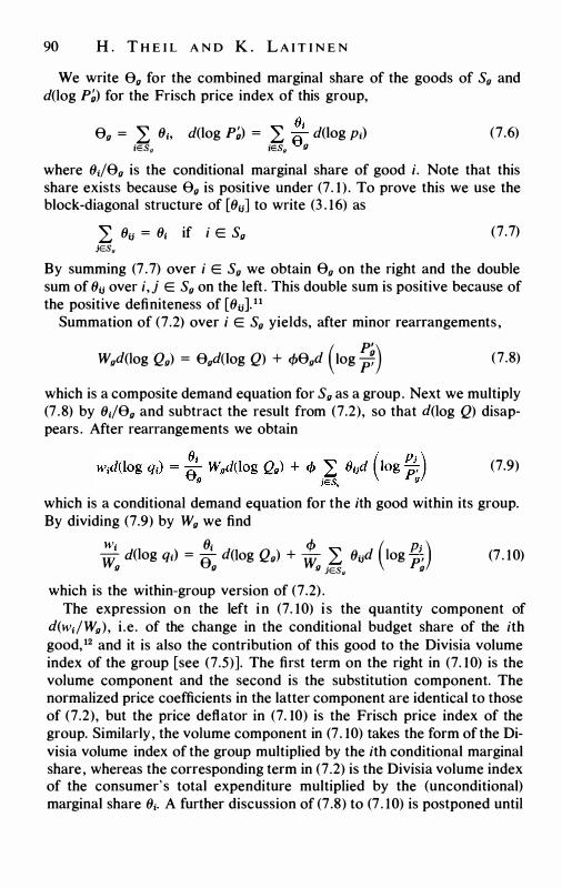
90 H . T H E I L A N D K . L A I T I N E N

We write eg for the combined marginal share of the goods of Sg and d(log P;) for the Frisch price index of this group,

eg = L 9;, d(log P;) = L !i d(log p;) iES!J iESu g

(7.6)

where 9;/8g is the conditional marginal share of good i. Note that this share exists because 8g is positive under (7 . 1 ) . To prove this we use the block-diagonal structure of [9u] to write (3 . 16) as

L 9u = 9; if i E Sg JES,

(7.7)

By summing (7 . 7) over i E Sg we obtain eg on the right and the double sum of 9u over i, j E Sg on the left . This double sum is positive because of the positive definiteness of [9u]. 11

Summation of (7.2) over i E Sg yields, after minor rearrangements ,

Wgd(log Qg) = 8gd{log Q) + </J8gd (tog ��) (7.8)

which is a composite demand equation for Sg as a group. Next we multiply (7 .8) by 9;/8g and subtract the result from (7.2), so that d(log Q) disap­pears . After rearrangements we obtain

(7.9)

which is a conditional demand equation for the ith good within its group. By dividing (7.9) by Wg we find

W; 9; </J ( PJ ) w d(log q;) = e d(tog Qg) + w :L 9ud 1og r g g g JESu g (7 . 10)

which is the within-group version of (7.2) . The expression on the left in (7. 10) is the quantity component of

d(w;/Wg), i .e. of the change in the conditional budget share of the ith good, 12 and it is also the contribution of this good to the Divisia volume index of the group [see (7.5)]. The first term on the right in (7. 10) is the volume component and the second is the substitution component. The normalized price coefficients in the latter component are identical to those of (7.2), but the price deftator in (7. 10) is the Frisch price index of the group. Similarly , the volume component in (7 . 10) takes the form of the Di­visia volume index of the group multiplied by the ith conditional marginal share, whereas the corresponding term in (7.2) is the Divisia volume index of the consumer's total expenditure multiplied by the (unconditional) marginal share 9;. A further discussion of (7 .8) to (7 . 10) is postponed until

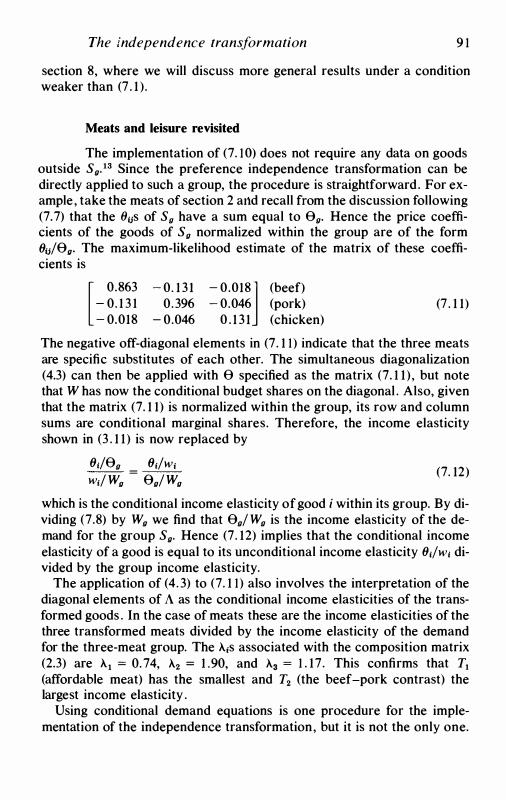
The independence transformation 9 1

section 8, where we will discuss more general results under a condition weaker than (7 . 1 ) .

Meats and leisure revisited

The implementation of (7. 1 0) does not require any data on goods outside Su. 13 Since the preference independence transformation can be directly applied to such a group, the procedure is straightforward. For ex­ample, take the meats of section 2 artd recall from the discussion following (7. 7) that the 8us of Su have a sum equal to 0u. Hence the price coeffi­cients of the goods of Su normalized within the group are of the form 8u/0u. The maximum-likelihood estimate of the matrix of these coeffi­cients is [ 0.863

- 0. 1 3 1 - 0.018

- 0. 1 3 1 - 0.018] (beef) 0.396 - 0.046 (pork)

- 0.046 0 . 1 3 1 (chicken) (7 . 1 1)

The negative off-diagonal elements in (7 . 1 1 ) indicate that the three meats are specific substitutes of each other. The simultaneous diagonalization (4.3) can then be applied with e specified as the matrix (7. 1 1 ) , but note that W has now the conditional budget shares on the diagonal . Also, given that the matrix (7. 1 1) is normalized within the group, its row and column sums are conditional marginal shares. Therefore, the income elasticity shown in (3 . 1 1 ) is now replaced by

8;/0u 8;/w; w;/Wu = 0u/Wu (7. 12)

which is the conditional income elasticity of good i within its group. By di­viding (7.8) by Wu we find that 0u/Wu is the income elasticity of the de­mand for the group Su. Hence (7 . 12) implies that the conditional income elasticity of a good is equal to its unconditional income elasticity 8;/w; di­vided by the group income elasticity.

The application of (4. 3) to (7. 1 1 ) also involves the interpretation of the diagonal elements of A as the conditional income elasticities of the trans­formed goods . In the case of meats these are the income elasticities of the three transformed meats divided by the income elasticity of the demand for the three-meat group. The A.;s associated with the composition matrix (2.3) are A.1 = 0. 74, A.2 = 1 .90, and A.3 = 1 . 17. This confirms that T1 (affordable meat) has the smallest and T2 (the beef-pork contrast) the largest income elasticity .

Using conditional demand equations is one procedure for the imple­mentation of the independence transformation, but it is not the only one.

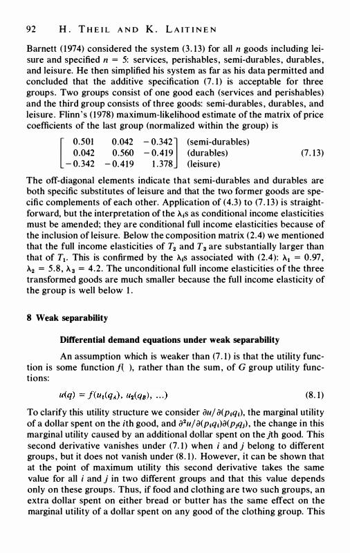
92 H . T H E I L A N D K . L A I T I N E N

Barnett ( 1974) considered the system (3 . 13) for all n goods including lei­sure and specified n = 5: services, perishables, semi-durables, durables , and leisure. He then simplified his system as far as his data permitted and concluded that the additive specification (7 . 1) is acceptable for three groups. Two groups consist of one good each (services and perishables) and the third group consists of three goods: semi-durables , durables, and leisure . Flinn's ( 1978) maximum-likelihood estimate of the matrix of price coefficients of the last group (normalized within the group) is [ 0.501

0.042 - 0.342

0.042 - 0.342] (semi-durables) 0.560 - 0.419 (durables)

- 0.419 1 .378 (leisure) (7 . 13)

The off-diagonal elements indicate that semi-durables and durables are both specific substitutes of leisure and that the two former goods are spe­cific complements of each other. Application of (4.3) to (7 . 13) is straight­forward, but the interpretation of the A1s as conditional income elasticities must be amended; they are conditional full income elasticities because of the inclusion of leisure. Below the composition matrix (2.4) we mentioned that the full income elasticities of T2 and T3 are substantially larger than that of T1 • This is confirmed by the A1s associated with (2.4): A1 = 0.97, A2 = 5.8, A3 = 4.2. The unconditional full income elasticities of the three transformed goods are much smaller because the full income elasticity of the group is well below 1 .

8 Weak separability

Differential demand equations under weak separability

An assumption which is weaker than (7 . 1) is that the utility func­tion is some function f( ), rather than the sum, of G group utility func­tions:

(8. 1)

To clarify this utility structure we consider au/ iJ(p1q1), the marginal utility of a dollar spent on the ith good, and iJ2u/ iJ(p1q1)iJ(pJq1) , the change in this marginal utility caused by an additional dollar spent on thejth good. This second derivative vanishes under (7. 1) when i and j belong to different groups, but it does not vanish under (8 . 1) . However, it can be shown that at the point of maximum utility this second derivative takes the same value for all i and j in two different groups and that this value depends only on these groups. Thus, if food and clothing are two such groups, an extra dollar spent on either bread or butter has the same effect on the marginal utility of a dollar spent on any good of the clothing group. This

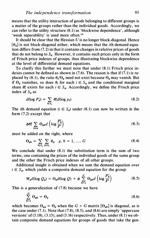
The independence transformation 93

means that the utility interaction of goods belonging to different groups is a matter of the groups rather than the individual goods . Accordingly, we can refer to the utility structure (8. 1 ) as 'blockwise dependence' , although 'weak separability' is used more often. 14

It should be clear that the Hessian U is no longer block-diagonal. Hence [8ii] is not block-diagonal either, which means that the ith demand equa­tion differs from (7. 2) in that it contains changes in relative prices of goods that do not belong to Su . However, it contains such prices only in the form of Frisch price indexes of groups, thus illustrating blockwise dependence at the level of differential demand equations.

To clarify this further we must note that under (8. 1 ) Frisch price in­dexes cannot be defined as shown in (7.6). The reason is that if (7. 1 ) is re­placed by (8. 1 ) , the ratio 8;/0u need not exist because eu may vanish. But if eu vanishes, so does 81 for each i E Su and the conditional marginal share flt exists for each i E Su. Accordingly , we define the Frisch price index of Su as

d(log P�) = L fltd(log Pi) (8.2) iES0

The ith demand equation (i E Su) under (8. 1 ) can now be written in the form (7.2) except that

</>8f L euhd (1og ��) hfg

must be added on the right, where

euh = L L 8ij g, h = 1 , . . . , o iES, iESh

(8.3)

(8.4)

We conclude that under (8. 1) the substitution term is the sum of two terms , one containing the prices of the individual goods of the same group and the other the Frisch price indexes of all other groups .

Additional insight is obtained when we sum the demand equation over i E Su, which yields a composite demand equation for the group:

G ( P' ) Wud(log Qu) = 0ud(log Q) + </> �1

euhd log / This is a generalization of (7.8) because we have

G L euh = eg h=l

(8.5)

(8.6)

which becomes 0uu = eu when the G x G matrix [euh] is diagonal , as is the case under (7. 1 ) . Note that (7.8), (8.5), and (8.6) are simply 'uppercase versions' of (3 . 1 8) , (3. 13) , and (3 . 16) respectively. Thus, under (8. 1 ) we ob­tain composite demand equations for groups of goods that take the gen-

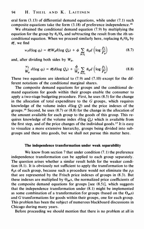
94 H . T H E I L A N D K . L A I T I N E N

era! form (3 . 13) of differential demand equations, while under (7. 1) such composite equations take the form (3. 18) of preference independence. 15

We obtained the conditional demand equation (7.9) by multiplying the equation for the group by 8;/8g and subtracting the result from the ith un­conditional equation. When we proceed similarly here, replacing 8;/8g by (ff, we find

w;d(log q1) = ()fWgd(log Qg) + <P L ()iid (1og ;�) (8.7) jE.'\, g

and, after dividing both sides by Wg,

� <P � ( � ) W d(log q;) = (ff d(log Qg) + W L.J ()iid log P' g g iES0 g

(8.8)

These two equations are identical to (7.9) and (7. 10) except for the dif­ferent notations of the conditional marginal shares.

The composite demand equations for groups and the conditional de­mand equations for goods within their groups enable the consumer to apply a two-stage budgeting procedure . First, he uses (8.5) for the change in the allocation of total expenditure to the G groups, which requires knowledge of the volume index d(log Q) and the price indexes of the groups .16 Second, he uses (8.7) or (8.8) for the change in the allocation of the amount available for each group to the goods of this group. This re­quires knowledge of the volume index d(log Qg) which is available from the first step, and of the price changes of the individual goods. 17 It is easy to visualize a more extensive hierarchy, groups being divided into sub­groups and these into goods, but we shall not pursue this matter here .

The independence transformation under weak separability

We know from section 7 that under condition (7 . 1 ) the preference independence transformation can be applied to each group separately . The question arises whether a similar result holds for the weaker condi­tion (8. 1 ) . It is obviously not sufficient to apply the transformation to the ()iis of each group, because such a procedure would not eliminate the p1s that are represented by the Frisch price indexes of groups in (8 .3) . But these indexes are multiplied by 8ghs, the normalized price coefficients of the composite demand equations for groups [see (8.5)], which suggests that the independence transformation under (8. 1) might be implemented as some combination of a transformation for groups (based on the eghs) and G transformations for goods within their groups, one for each group. This problem has been the subject of numerous blackboard discussions in Chicago during many years .

Before proceeding we should mention that there is no problem at all in

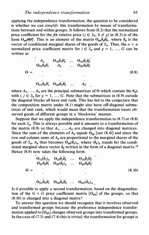
The independence transformation 95

applying the independence transformation; the question to be considered is whether we can simplify this transformation by means of transforma­tions between and within groups. It follows from (8.2) that the normalized price coefficient for the jth relative price U E Sh, h 1' g) in (8 .3) is of the form euh6'f87. This is an element of the matrix euhOufJJi, where Ou is the vector of conditional marginal shares of the goods of S9• Thus, the n x n normalized price coefficient matrix for i E S9 and g = 1 , . . . , G can be written as

Ai 012818� ew818/; 021828; A2 02G820/;

0 = (8.9)

0G10G8; 0G28G82 AG where Ai. . . . , AG are the principal submatrices of e which contain the 8vs with i, j E S9 for g = 1 , . . . , G. Note that the submatrices in (8.9) outside the diagonal blocks all have unit rank. This has led to the conjecture that the composition matrix under (8. 1 ) might also have off-diagonal subma­trices of unit rank, which would mean that the transformation treats ob­served goods of different groups in a 'blockwise' manner.

Suppose that we apply the independence transformation to (8.7) or (8.8) for each S9• This is always possible and it amounts to a transformation of the matrix (8.9) so that Ai . . . . , AG are changed into diagonal matrices . Since the sum of the elements of A9 equals 099 [see (8.4)] and since the row and column sums of Au are proportional to the marginal shares of the goods of S9, A9 thus becomes 0u9(09)11, where (09)11 stands for the condi­tional marginal share vector 09 written in the form of a diagonal matrix. 18 Hence (8.9) now takes the following form:

011(01)11 0120102 ew810/; 021028; 022(02)11 02G020/;

0 = (8. 10)

eG10Go; 0G20G02 0GG(OG)11 Is it possible to apply a second transformation, based on the diagonaliza­tion of the G x G price coefficient matrix [09h] of the groups , so that (8. 10) is changed into a diagonal matrix?

To answer this question we should recognize that it involves observed and transformed groups because the preference independence transfor­mation applied to [09h] changes observed groups into transformed groups. In the case of (7.3) and (7.4) this is trivial; the transformation for groups is

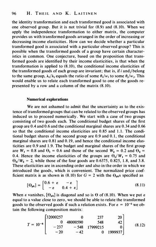
96 H . T H E I L A N D K . L A I T I N E N

the identity transformation and each transformed good is associated with one observed group. But it is not trivial for (8.9) and (8. 10) . When we apply the independence transformation to either matrix , the computer provides us with transformed goods arranged in the order of increasing or decreasing income elasticities . How can we decide whether a particular transformed good is associated with a particular observed group? This is possible when the transformed goods of a group have certain character­istics in common. One conjecture, based on the proposition that trans­formed goods are identified by their income elasticities , is that when the transformation is applied to (8. 10), the conditional income elasticities of the transformed goods of each group are invariant ; that is, if i andj belong to the same group, >..;/'Ai equals the ratio of some 8;/w; to some ()i/wi. This would enable us to relate each transformed good to one of the goods re­presented by a row and a column of the matrix (8. 10).

Numerical explorations

We are not ashamed to admit that the uncertainty as to the exis­tence of transformed groups that can be related to the observed groups has induced us to proceed numerically . We start with a case of two groups consisting of two goods each. The conditional budget shares of the first group are 0.4 and 0.6 and the conditional marginal shares are 0.34 and 0.66 so that the conditional income elasticities are 0.85 and 1 . 1 . The condi­tional budget shares of the second group are 0.9 and 0. 1 , the conditional marginal shares are 0.8 1 and 0. 19, and hence the conditional income elas­ticities are 0.9 and 1 .9. The budget and marginal shares of the first group are W1 = 0.8 and e1 = 0.6 and those of the second W2 = 0.2 and e2 = 0.4. Hence the income elasticities of the groups are 0i/ W1 = 0. 75 and e2/W2 = 2, while those of the four goods are 0.6375, 0.825, 1 .8, and 3 .8. These elasticities are in ascending order and also in the order in which we introduced the goods , which is convenient. The normalized price coef­ficient matrix is as shown in (8. 10) for G = 2 with the e0hs specified as

[e J = [0.6 + e - e J oh - e 0.4 + e (8. 1 1)

When e vanishes , [e0h] is diagonal and so is e of (8. 10). When we put e equal to a value close to zero , we should be able to relate the transformed goods to the observed goods if such a relation exists . For e = 10-s we ob­tain the following composition matrix : f 32000257

T = 10-s 0

- 237 - 20

0 48000590

- 548 - 42

237 201 548 42

179992 15 0 0 1999937

(8. 12)

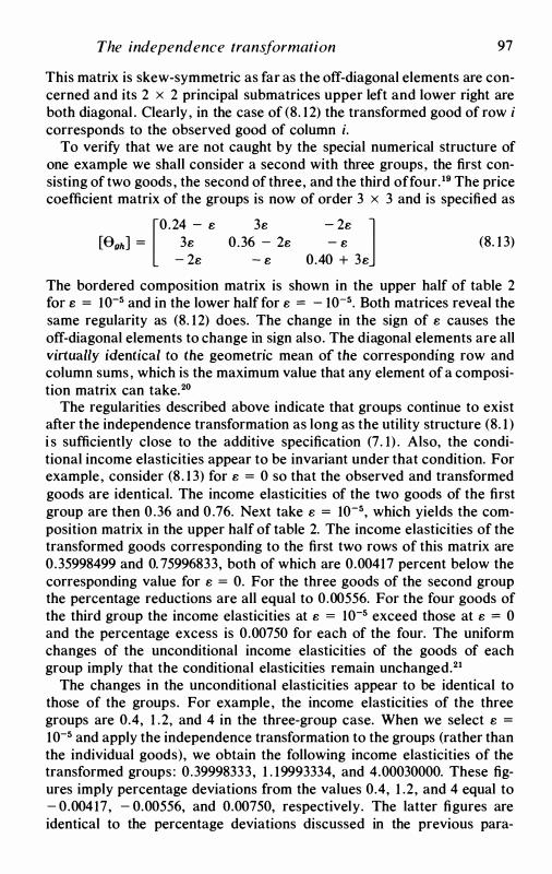
The independence transformation 97

This matrix is skew-symmetric as far as the off-diagonal elements are con­cerned and its 2 x 2 principal submatrices upper left and lower right are both diagonal . Clearly, in the case of (8. 12) the transformed good of row i corresponds to the observed good of column i.

To verify that we are not caught by the special numerical structure of one example we shall consider a second with three groups, the first con­sisting of two goods , the second of three, and the third offour.19 The price coefficient matrix of the groups is now of order 3 x 3 and is specified as [0.24 - e 3e - 2e ]

[euh] = 3e 0.36 - 2e - e - 2e - e 0.40 + 3e

(8. 1 3)

The bordered composition matrix is shown in the upper half of table 2 for e = 10-s and in the lower half for e = - 10-s. Both matrices reveal the same regularity as (8. 12) does. The change in the sign of e causes the off-diagonal elements to change in sign also. The diagonal elements are all virtually identical to the geometric mean of the corresponding row and column sums , which is the maximum value that any element of a composi­tion matrix can take. 20

The regularities described above indicate that groups continue to exist after the independence transformation as long as the utility structure (8. 1 ) i s sufficiently close to the additive specification (7 . 1) . Also, the condi­tional income elasticities appear to be invariant under that condition. For example, consider (8 . 1 3) for e = 0 so that the observed and transformed goods are identical. The income elasticities of the two goods of the first group are then 0 .36 and 0 .76. Next take e = 10-s, which yields the com­position matrix in the upper half of table 2. The income elasticities of the transformed goods corresponding to the first two rows of this matrix are 0.35998499 and 0. 75996833, both of which are 0.00417 percent below the corresponding value for e = 0. For the three goods of the second group the percentage reductions are all equal to 0.00556. For the four goods of the third group the income elasticities at e = 10-s exceed those at e = 0 and the percentage excess is 0.00750 for each of the four. The uniform changes of the unconditional income elasticities of the goods of each group imply that the conditional elasticities remain unchanged.21

The changes in the unconditional elasticities appear to be identical to those of the groups. For example, the income elasticities of the three groups are 0.4, 1 .2, and 4 in the three-group case. When we select e = 10-s and apply the independence transformation to the groups (rather than the individual goods), we obtain the following income elasticities of the transformed groups : 0.39998333, 1 . 19993334, and 4.00030000. These fig­ures imply percentage deviations from the values 0.4, 1 .2, and 4 equal to - 0.004 17, - 0.00556, and 0.00750, respectively. The latter figures are identical to the percentage deviations discussed in the previous para-

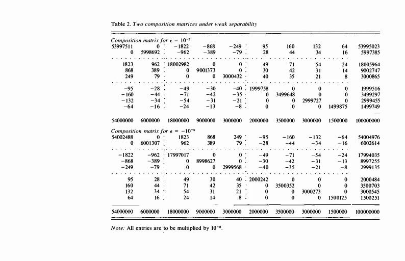
Table 2. Two composition matrices under weak separability

Composition matrix for E = 10-5 5399751 1 0 . - 1822

0 5998692 : -962 .

.. . . . . . . . .

1823 962 . 18002982 868 389 : 0 249 79 . 0

. . . . . -95 -28 -49

- 160 -44 -71 - 132 -34 -54 -64 - 1 6 -24

54000000 6000000 18000000

Composition matrix for E = - 10-5 54002488

0

- 1 822 -868 -249

95 160 132 64

54000000

0 .

6001 307 : . . . . • , •

-962 -389 :

-79 .

28 44 34 16

6000000

1823 962

17997017 0 0

49 7 1 54 24

18000000

-868 -389

0 9001373

0

-30 -42 - 3 1 - 1 3

9000000

868 389

0 8998627

0

30 42 3 1 14

9000000

Note: All entries are to be multiplied by 10-s.

-249 .

-79 : 0 .

0 : 3000432 .

. . . . .

-40 : -35 .

-21 -8 :

3000000

249 .

79 : 0 .

0 : 2999568 .

. . . .

95 28

49 30 40

1999758 0 0 0

2000000

-95 -28

-49 -30 -40

40 : 2000242 35 0 21 0

8 0

3000000 2000000

160 132 64 53995023 44 34 16 5997385

7 1 54 24 18005964 42 3 1 14 9002747 35 21 8 3000865

0 0 0 1999516 3499648 0 0 3499297

0 2999727 0 2999455 0 0 1499875 1499749

3500000 3000000 1500000 100000000

- 160 - 1 32 -64 54004976 -44 -34 - 16 6002614

-71 -54 -24 17994035 -42 - 3 1 - 13 8997255 -35 -21 -8 29991 35

0 0 0 2000484 3500352 0 0 3500703

0 3000273 0 3000545 0 0 1500125 1 500251

3500000 3000000 1500000 100000000

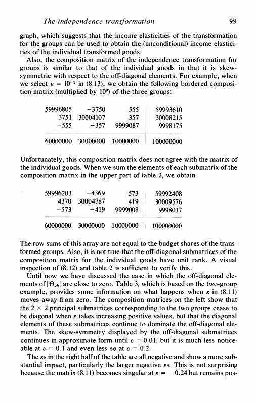
The independence transformation 99

graph, which suggests that the income elasticities of the transformation for the groups can be used to obtain the (unconditional) income elastici­ties of the individual transformed goods.

Also, the composition matrix of the independence transformation for groups is similar to that of the individual goods in that it is skew­symmetric with respect to the off-diagonal elements. For example , when we select e = 10-5 in (8. 1 3) , we obtain the following bordered composi­tion matrix (multiplied by 108) of the three groups:

59996805 375 1

-555

-3750 30004107

-357

555 357

9999087

60000000 30000000 10000000

599936 10 300082 15 9998 175

100000000

Unfortunately, this composition matrix does not agree with the matrix of the individual goods. When we sum the elements of each submatrix of the composition matrix in the upper part of table 2, we obtain

599%203 -4369 4370 30004787 -573 -419

573 419

9999008

60000000 30000000 1 0000000

59992408 30009576

9998017

100000000

The row sums of this array are not equal to the budget shares of the trans­formed groups. Also, it is not true that the off-diagonal submatrices of the composition matrix for the individual goods have unit rank. A visual inspection of (8 . 12) and table 2 is sufficient to verify this .

Until now we have discussed the case in which the off-diagonal ele­ments of [0gh] are close to zero. Table 3, which is based on the two-group example, provides some information on what happens when e in (8. 1 1) moves away from zero . The composition matrices on the left show that the 2 x 2 principal submatrices corresponding to the two groups cease to be diagonal when e takes increasing positive values, but that the diagonal elements of these submatrices continue to dominate the off-diagonal ele­ments . The skew-symmetry displayed by the off-diagonal submatrices continues in approximate form until e = 0.0 1 , but it is much less notice­able at e = 0. 1 and even less so at e = 0.2.

The es in the right half of the table are all negative and show a more sub­stantial impact, particularly the larger negative es. This is not surprising because the matrix (8. 1 1 ) becomes singular at e = - 0.24 but remains pos-

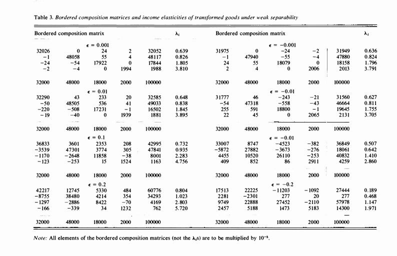
Table 3. Bordered composition matrices and income elasticities of transformed goods under weak separability

Bordered composition matrix A1 Bordered composition matrix A1 E = 0.001 E = -0.001

32026 0 24 2 32052 0.639 31975 0 -24 -2 3 1949 0.636 - 1 48058 55 4 48 1 17 0.826 - 1 47940 -55 -4 47880 0.824

-24 -54 17922 0 17844 1 .805 24 55 1 8079 0 18158 1 .796 -2 -4 0 1994 1988 3.810 2 4 0 2006 2013 3 .791

32000 48000 18000 2000 100000 32000 48000 18000 2000 100000

E = 0.01 E = -0.01 32290 43 233 20 32585 0.648 3 1777 46 -243 -21 3 1560 0.627

-50 48505 536 4 1 49033 0.838 -54 473 18 -558 -43 46664 0.81 1 -220 -508 17231 - 1 16502 1 .845 255 591 18800 - 1 19645 1 .755

- 19 -40 0 1939 1881 3.895 22 45 0 2065 2131 3.705

32000 48000 18000 2000 100000 32000 48000 18000 2000 100000

E = 0. 1 E = -0.01 36833 3601 2353 208 42995 0.732 33007 8747 -4523 -382 36849 0.507

-3539 47301 3774 305 47841 0.935 -5872 27882 - 3673 -276 1 8061 0.642 - 1 170 - 2648 1 1858 -38 8001 2.283 4455 10520 261 10 -253 40832 1 .410

- 123 -253 15 1524 1 163 4.756 409 852 86 291 1 4259 2.860

32000 48000 1 8000 2000 100000 32000 48000 18000 2000 100000

E = 0.2 E = -0.2 42217 12745 5330 484 60776 0.804 175 13 22225 - 1 1203 - 1092 27444 0. 189

-8755 38480 42 14 354 34293 1 .023 2281 -2301 277 20 277 0.468 - 1297 - 2886 8422 -70 4169 2.803 9749 22888 27452 -21 10 57978 1 . 147

- 166 -339 34 1232 762 5.720 2457 5188 1473 5183 14300 1 .971

32000 48000 18000 2000 100000 32000 48000 18000 2000 100000

Note: All elements of the bordered composition matrices (not the >.1s) are to be multiplied by 10-•.

The independence transformation 1 0 1

itive definite at e = 0.24. The composition matrix for e = -0 . 2 contains a negative diagonal element and the smallest root (A1 = 0 . 189) is much smaller than that at e = - 0. 1 . The behaviour of the A;S as functions of e is otherwise very smooth. When e moves toward - 0.24, A1 converges to zero, which implies that the conditional income elasticities cannot be in­variant when e is not close to zero.

The numerical evidence discussed above suggests that when weak sep­arability is treated by means of a Taylor expansion from the point of strong separability, the leading term (but not the next terms) of this ex­pansion has a blockwise structure . The mathematical form of this struc­ture merits a further investigation.

A P PE N D I X

A Derivations for the preference independence transformation

Invariance constraints

Let each dollar spent on the jth observed good imply ru dollars spent on the ith transformed good, where ru is to be determined but is not yet defined. When p1q1 dollars are spent on the jth observed good, the expenditure on the ith transformed good is thus rup1q1 dollars insofar as this expenditure originates with the jth observed good. Summation over j yields L1 rup1q1' which is the total amount spent on the ith transformed good. Next, by summing this over i, we obtain L1 (L; ru)p1q1' the total amount spent on all n transformed goods. We require the total amount spent to be invariant (equal to M = L1 p1q1), which implies L; ru = 1 for each j or

i'R = i' (A. I) where i' = [ 1 . . . 1 ] and R is the n x n matrix [rul

Since the amount spent on the ith transformed good is L1 rup1q1' its budget share equals L1 rup1q1/ M = L1 ruw1• We write this as

Wrt = RWi (A . 2)

where Wr is the diagonal matrix with the budget shares wri , . . . , Wrn of the transformed goods on the diagonal .

We write 7T and K for the n-element column vectors whose ith elements are d(log p;) and d(log q1) , respectively . Let the logarithmic price and quantity changes of the transformed goods be linear transformations of their observed counterparts,

7Tr = S7T, Kr = SK (A.3)

1 02 H . T H E I L A N D K . L A I T I N E N

in such a way that the Divisia indexes (3.5) and (3.6) are invariant .22 The index (3 .5) equals i'Wrr and its transformed counterpart is i' Wrrrr = i' WrS1T, which is equal to i' WR' S7T in view of (A.2). The invariance of this index thus amounts to

R'S = I (A.4)

which implies R' = s-1 • Since R' i = i follows from (A. I ) , this yields s-li = i and hence, after premultipJication by S, 23

Si = i (A.5)

Note that (A.4) requires R to be nonsingular. The singular case will be considered at the end of this section.

The diagonalization

We write (3. 16) as 8i = 8, where 8 = [81] is the marginal share vector. The Frisch price index (3. 10) can then be written as 8'1T = i'81T and the demand system (3. 13) for i = 1 , . . . , n as

WK = (i'WK)8i + <f>8(1 - u'8)7T (A.6)

where i 'WK = d(log Q). We premultiply (A.6) by R: RWK = (i'WK)R8i + <f>R8(1 - u'8)7T

The left-hand side equals RWR' SK = RWR' Kr [see (A.3) and (A.4)]. When we proceed similarly on the right, using (A. 1 ) also, we obtain

RWR'Kr = (i' WK)(R8R')i + <f>R8R'[I - ii'(R8R')]1Tr (A.7)

Since the Divisia volume index is invariant by construction (i' WK = i'WrKr), (A.7) is a demand system of the same form as (A.6), with price and quantity changes 1Tr and Kr, provided RWR' on the left can be identi­fied with the diagonal budget share matrix Wr. The new normalized price coefficent matrix is R8R' , 24 which occurs in the same three places in (A.7) as 8 does in (A.6). Therefore, two conditions are required in order that (A. 7) be a differential demand system in preference inde­pendent form:

RWR' = Wr, R8R' = diagonal (A.8)

These are two conditions on R, which must satisfy (A. I ) also. We proceed to prove that these three conditions are satisfied by

(A.9)

where X and (X-1i)<l are defined as in the first subsection of section 4. Condition (A. I) in the form R' i = i is satisfied by (A.9) because X(X-1i)<li = xx-1i = i. Also, RWR' = (x-1i)<lX'WX(X-1i)<l = (X-1i)l,

The independence transformation 1 03

where the last step is based on (4.3). Therefore, the first condition in (A.8) is satisfied in the following form:

RWR' = WT = (X-1t)l = diagonal

The second condition is satisfied in the form

(A. 10)

R0R' = (X-1t)lA = diagonal (A. 1 1 )

which follows from (A .9) and e = (X')-1AX-1 [see (4.3)]. The first term on the right in (A.7) shows that (R0R')t is the marginal share vector of the transformed goods; hence the diagonal elements of the matrix product (A. 1 1 ) are these marginal shares.

To verify the composition matrix (4.4) we recall from the discussion preceding (A. 1) that the expenditure on the ith transformed good is ruPJqJ dollars insofar as it originates with thejth observed good. By dividing this by M we obtain riJWJ> which is the budget share of the ith transformed good insofar as it originates with the jth observed good . This ruwJ is the (i, j)th element of the composition matrix T and obviously also the (i, j)th element of RW, so that T = RW. We then obtain (4.4) from RW = (X-1i)<lX'(X')-1x-1 = (X-1ihx-1 , where use is made of (A.9) and W = (X')-1x-1 [see (4.3)]. Post-multiplication of T = RW by t gives Ti = RWt = WTL [see (A.2)] ; hence the row sums of T are the budget shares of the transformed goods. Also, i 'T = i'RW = i'W, which proves that the column sums of T are the budget shares of the observed goods.

Multiple roots and near-multiple roots

The solution (A.9) is unique when there are no multiple roots [i.e. no equal diagonal elements in A in (4.3)].25 We proceed to consider a pair of multiple roots , A.1 = A.2 I- A.; for i > 2. The characteristic vectors X1 and x2 associated with the multiple root are not uniquely determined; we may post-multiply [x1 x2] by an arbitrary 2 x 2 orthogonal matrix and the two vectors which emerge satisfy (4. 1) and the normalization rules . This inde­terminacy of x1 and x2 implies a similar indeterminacy of the budget and marginal shares of the two transformed goods. If A.3, • • • , An are distinct , the budget and marginal shares of the last n - 2 transformed goods are well defined, so that the combined budget share and the combined marginal share of the first two are also well defined. Also, the first two rows of the composition matrix are indeterminate, although constrained by the fact that their sum is determinate . This means that the two trans­formed goods with equal income elasticities are identical or, equivalently , that they behave like one good so that there are only n - 1 transformed goods.

We proceed to discuss the perturbations of table 1 , the last column of which contains the marginal shares of the transformed goods. We perturb

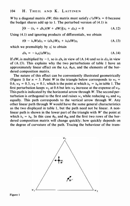
1 04 H . T H E I L A N D K . L A I T I N E N

W by a diagonal matrix dW; this matrix must satisfy t' (dW)t = 0 because the budget shares add up to 1 . The perturbed version of (4. 1) is

[e - (A; + dA;)(W + dW)](x; + dx;) = 0

Using (4. 1) and ignoring products of differentials , we obtain

(8 - A.;W)dx; = (dA.;)Wx; + A;(dW)x; which we premultiply by xi to obtain

dA.; = - A.;xi(dW)x;

(A. 12)

(A. 13)

(A. 14)

If dW; is multiplied by - I , so is dA.; in view of (A. 14) and so is dx1 in view of (A. 13). This explains why the two perturbations of table 1 have an approximately linear effect on the A.;s, 9r;S, and the elements of the bor­dered composition matrix.

The nature of this effect can be conveniently illustrated geometrically (Figure 1) for n = 3 . Point W in the triangle below corresponds to w1 = 0.6, w2 = 0.3, w3 = 0. 1 , which is the point at which A.1 = A.2 in table 1 . The first perturbation keeps w1 at 0.6 but lets w2 increase at the expense of w3•

This path is indicated by the horizontal arrow through W. The second per­turbation is orthogonal to the first and raises w1 while reducing w2 and w3

equally . This path corresponds to the vertical arrow through W. Any other linear path through W would have the same general characteristics as the two displayed in table 1 , but the path need not be linear. A non­linear path is shown in the lower part of the triangle with W' the point at which A.1 = A.2• In this case 9r1 and 9T2 and the first two rows of the bor­dered composition matrix will change quickly; how quickly depends on the degree of curvature of the path. Tracing the behaviour of the trans-

Figure 1

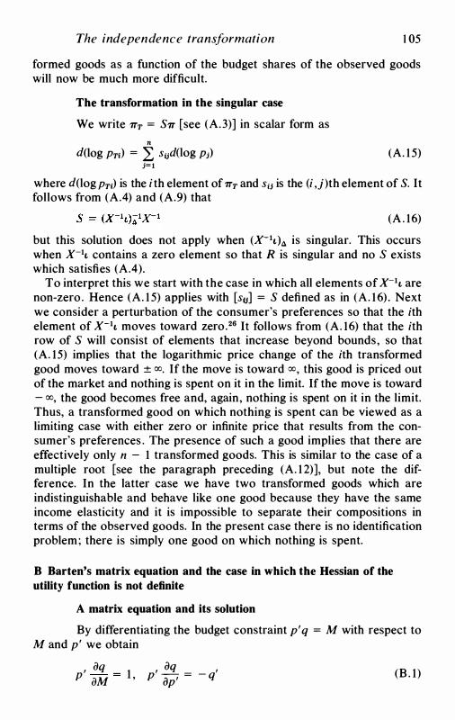
The independence transformation 1 05

formed goods as a function of the budget shares of the observed goods will now be much more difficult.

The transformation in the singular case

We write 1Tr = S7T [see (A.3)] in scalar form as n

d(log Pr1) = L sud(log P;) j=!

(A. 1 5)

where d(log Pr1) is the ith element of 1Tr and siJ is the (i ,j)th element of S. It follows from (A.4) and (A.9) that

(A. 16)

but this solution does not apply when (X-'ih is singular. This occurs when x-1i contains a zero element so that R is singular and no S exists which satisfies (A.4).

To interpret this we start with the case in which all elements of x-1i are non-zero. Hence (A. 1 5) applies with [s0] = S defined as in (A. 16) . Next we consider a perturbation of the consumer's preferences so that the ith element of x-1i moves toward zero.26 It follows from (A. 16) that the ith row of S will consist of elements that increase beyond bounds, so that (A. 15) implies that the logarithmic price change of the ith transformed good moves toward ± oo. If the move is toward oo, this good is priced out of the market and nothing is spent on it in the limit. If the move is toward - oo, the good becomes free and, again, nothing is spent on it in the limit. Thus, a transformed good on which nothing is spent can be viewed as a limiting case with either zero or infinite price that results from the con­sumer's preferences . The presence of such a good implies that there are effectively only n - 1 transformed goods. This is similar to the case of a multiple root [see the paragraph preceding (A. 1 2)], but note the dif­ference. In the latter case we have two transformed goods which are indistinguishable and behave like one good because they have the same income elasticity and it is impossible to separate their compositions in terms of the observed goods. In the present case there is no identification problem; there is simply one good on which nothing is spent.

B Barten's matrix equation and the case in which the Hessian of the utility function is not definite

A matrix equation and its solution

By differentiating the budget constraint p' q = M with respect to M and p ' we obtain

, aq p aM

1 , aq ' p i}p' = - q' (B . 1)

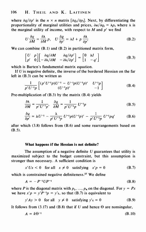
1 06 H . T H E I L A N D K . L A I T I N E N

where oq/op' is the n x n matrix [oqi/op;] . Next, by differentiating the proportionality of marginal utilities and prices, au/oqi = >..pi where >.. is the marginal utility of income, with respect to M and p' we find

(B .2)

We can combine (B . 1 ) and (B .2) in partitioned matrix form,

[u p] [ aq/aM aq/ap'] _

[o >..1 J p' o - a>../aM - a>../ap' - 1 - q' (B.3)

which is Barten's fundamental matrix equation. If U is negative definite , the inverse of the bordered Hessian on the far

left in (B.3) can be written as

1 [(p' u-1p)u-1 _ u-1p( u-1p) ' p' U-1p (U-1p) '

u-1PJ - 1

Pre-multiplication of (B.3) by the matrix (B.4) yields

1 u-1 p' u-1p p

(B.4)

(B.5)

;;, = >..u-1 - p' �-1P u-1p(u-1p)' - p' �-1P

u-1pq' (B.6)

after which (3.8) follows from (B.6) and some rearrangements based on (B .5) .

What happens if the Hessian is not definite?

The assumption of a negative definite U guarantees that utility is maximized subject to the budget constraint, but this assumption is stronger than necessary . A sufficient condition is

x' Ux < 0 for all x "I 0 satisfying x' p = 0 which is constrained negative definiteness.27 We define

A = - p-1up-1

(B.7)

(B.8) where P is the diagonal matrix with Pi . . . . , Pn on the diagonal . For y = Px we have x'p = y'P-1p = y't, so that (B.7) is equivalent to

y' Ay > 0 for all y "I 0 satisfying y' t = 0 (B.9)

It follows from (3. 17) and (B.8) that if U and hence e are nonsingular,

A = ke-1 (B . 10)

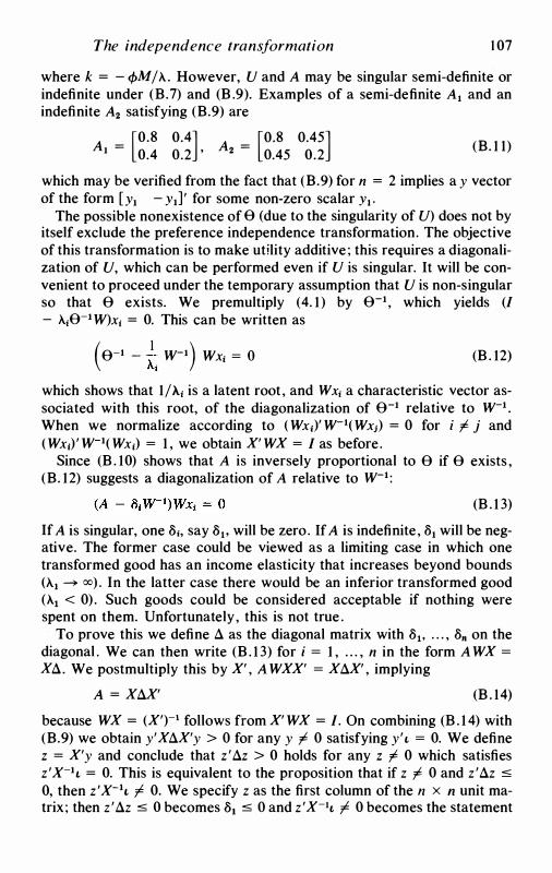
The independence transformation 1 07

where k = - <f>M / >.. . However, U and A may be singular semi-definite or indefinite under (B.7) and (B .9). Examples of a semi-definite Ai and an indefinite A2 satisfying (B.9) are

Ai = [0.8 0.4] A2 = [0.8 0.45] 0.4 0.2 ' 0.45 0.2

(B. 1 1)

which may be verified from the fact that (B.9) for n = 2 implies a y vector of the form [Yi - Yi] ' for some non-zero scalar Yi ·

The possible nonexistence of 0 (due to the singularity of U) does not by itself exclude the preference independence transformation. The objective of this transformation is to make utility additive ; this requires a diagonali­zation of U, which can be performed even if U is singular. It will be con­venient to proceed under the temporary assumption that U is non-singular so that 0 exists. We premultiply (4. 1 ) by e-i, which yields (I - >..;e-i W)x; = 0. This can be written as

( e-i - �; w-i) Wx1 = o (B . 12)

which shows that 1/>..; is a latent root , and Wx; a characteristic vector as­sociated with this root, of the diagonalization of e-i relative to w-i . When we normalize according to (Wx1)' W-i(Wx;) = 0 for i I j and (Wx1) ' w-i(Wx1) = 1 , we obtain X' WX = I as before.

Since (B . 10) shows that A is inversely proportional to 0 if 0 exists , (B. 12) suggests a diagonalization of A relative to w-i:

(B . 1 3)

If A is singular, one S1, say Si. will be zero. If A is indefinite , Si will be neg­ative. The former case could be viewed as a limiting case in which one transformed good has an income elasticity that increases beyond bounds (>..i ....,. oo) . In the latter case there would be an inferior transformed good (A.1 < 0) . Such goods could be considered acceptable if nothing were spent on them. Unfortunately, this is not true .

To prove this we define .l as the diagonal matrix with Si. . . . , Sn on the diagonal . We can then write (B . 1 3) for i = 1 , . . . , n in the form AWX = X.l. We postmultiply this by X' , A WXX' = X.lX' , implying

A = X.lX' (B . 14)

because WX = (X')-i follows from X' WX = I. On combining (B . 1 4) with (B.9) we obtain y'X.lX'y > 0 for any y I 0 satisfying y'i = 0. We define z = X'y and conclude that z ' .lz > 0 holds for any z I 0 which satisfies z ' x-iL = 0. This is equivalent to the proposition that if z I 0 and z ' .lz :s 0, then z 'x-ii I 0. We specify z as the first column of the n x n unit ma­trix ; then z ' .lz :s 0 becomes S1 :s 0 and z 'X-1i I 0 becomes the statement

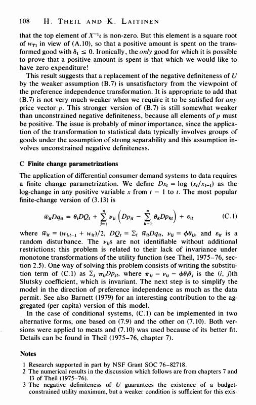
108 H . T H E I L A N D K . L A I T I N E N

that the top element of x-1i is non-zero. But this element is a square root of wTI in view of (A. 10), so that a positive amount is spent on the trans­formed good with 81 s: 0. Ironically , the only good for which it is possible to prove that a positive amount is spent is that which we would like to have zero expenditure !

This result suggests that a replacement of the negative definiteness of U by the weaker assumption (B. 7) is unsatisfactory from the viewpoint of the preference independence transformation. It is appropriate to add that (B.7) is not very much weaker when we require it to be satisfied for any price vector p. This stronger version of (B. 7) is still somewhat weaker than unconstrained negative definiteness, because all elements of p must be positive. The issue is probably of minor importance, since the applica­tion of the transformation to statistical data typically involves groups of goods under the assumption of strong separability and this assumption in­volves unconstrained negative definiteness.

C Finite change parametrizations

The application of differential consumer demand systems to data requires a finite change parametrization. We define Dx1 = log (xtf x1-1) as the log-change in any positive variable x from t - 1 to t. The most popular finite-change version of (3 . 13) is

WuDqu = 61DQ1 + � Vu ( Dp;t - �1 6kDPkt) + Bu (C . 1)

where Wu = (w;,1-1 + w11)/2, DQ1 = �; wuDqu, vu = <f>6u, and Bu is a random disturbance. The vus are not identifiable without additional restrictions; this problem is related to their lack of invariance under monotone transformations of the utility function (see Theil, 1975-76, sec­tion 2.5) . One way of solving this problem consists of writing the substitu­tion term of (C. 1) as �; 7TuDP;1, where 7Tu = vu - </>616; is the (i, j)th Slutsky coefficient , which is invariant. The next step is to simplify the model in the direction of preference independence as much as the data permit . See also Barnett ( 1979) for an interesting contribution to the ag­gregated (per capita) version of this model .

In the case of conditional systems, (C. 1 ) can be implemented in two alternative forms, one based on (7.9) and the other on (7. 10) . Both ver­sions were applied to meats and (7 . 10) was used because of its better fit. Details can be found in Theil ( 1975-76, chapter 7) .

Notes

1 Research supported in part by NSF Grant SOC 76-827 18. 2 The numerical results in the discussion which follows are from chapters 7 and

13 of Theil ( 1975-76). 3 The negative definiteness of U guarantees the existence of a budget­

constrained utility maximum, but a weaker condition is sufficient for this exis-

The independence transformation 1 09

tence . In appendix B we analyse some implications of this weaker condition. 4 This may be verified by writing the substitution term of (3 . 13) as a multiple </> of

L:; 8;,;d(log p;) - 81d(log P') [see (3 . 16)]. Summation of this expression over i yields zero because of the symmetry of [8;.;], (3. 16), and L:1 81 = I .

5 The derivative aA./aM equals the reciprocal of p ' u-•p, which is obtained by solving Barten' s fundamental matrix equation . This matrix equation and its so­lution are given in appendix B .

6 Equation (3. 16) follows from (3 . 15) and 81 = (A./<f>M)p1 L:; u1ip1, which is ob­tained by solving Barten's fundamental matrix equation.

7 This definition differs from Hicks' which is based on the total substitution ef­fect. Houthakker's definition is more useful for our present purposes.

8 That is, 81 equals the ratio of a(p1q1)/az to aC/az, where z = output. If the firm maximizes profit under competitive conditions on the supply side, 81 equals the additional expenditure on input i caused by an extra dollar of output revenue , which is more directly comparable to (3 .2). The l/J in (5. 1 ) is a curvature mea­sure of the logarithmic cost function ; it is positive, implying -1" < 0 in (5 . 1) , to be compared with </> < 0 in (3. 13) .

9 Hall ( 1973) has shown that under output independence the multi-product firm can be split up into m single-product firms, each making one of the products of the multi-product firm, in such a way that when the single-product firms inde­pendently maximize profits , they supply the same rate of output and use the same total quantity of each input as the multi-product firm.

IO This problem does not arise when all variables are expressed in the same unit. (This applies to Stone's ( 1947) application in which all variables are in dollars per year.) However, even in that case we obtain different results when we measure the variables from their natural zeros or from their means.

I I Also note that when the group indexes in (7.5) and (7.6) are weighted with the group budget and marginal shares W0 and 00, respectively , we obtain the in­dexes (3.6) and (3 . 1 0) which refer to the budget as a whole.

12 The other components are ( w;/ W0)d(log p1) and - ( w;/ W0)d(log W0M). The first of these is the price component of the change in the conditional budget share and the second is the component which is attributable to the change in the amount spent on the group. This result should be viewed as a within-group ver­sion of (3 . 12).

13 The implementation does require a parametrization; see appendix C for this matter.

14 The analogous constraint on the input structure of a firm was considered by Macurdy ( 1975).

15 Additional 'uppercase extensions' can be formulated. We may define S0 and Sh as specific substitutes (complements) when 00h in (8.5) is negative (positive). Under (7 . 1 ) no group is a specific substitute or complement of any other group. Also, no group can be inferior under (7. 1 ) because 0g > 0, but inferior groups can exist under (8. 1 ) .

16 The required price indexes of the groups include both Divisia and Frisch price indexes. The reason is that the logarithmic change in the amount spent on S9 equals d(log P9) + d(log Qg), where d(log P0) (no prime !) is the Divisia price index of S9• This index is obtained by substituting p1 for q1 in (7.5).

17 When random disturbances are added to the demand equations, the separation of the allocation into two steps requires the disturbances of the composite de­mand equations for groups of goods to be uncorrelated with those of the condi­tional equations. It can be shown that this is indeed the case under rational random behaviour; this theory implies that disturbances of conditional demand equations of different groups are also uncorrelated.

18 Strictly speaking, we should use a notation indicating that these conditional

1 1 0 H . T H E I L A N D K . L A I T I N E N

marginal shares refer to goods obtained from the independence transformation applied to the group, but we prefer not to do so to simplify the notation. It is, of course, possible that the G group utility functions (8. 1 ) are additive in their arguments, in which case (8.9) takes the form (8. 10) without any intermediate transformation. This special case was considered particularly by Pearce ( 1961 ; 1964). In the discussion later in this section we shall proceed as if (8. 10) refers to observed goods.

19 The budget shares of the groups are specified as 0.6, 0.3, and 0. 1 ; the marginal shares implied by (8. 13) are 0.24, 0.36, and 0.40 for any value of e, so that the income elasticities are 0.4, 1 .2, and 4. The conditional budget shares are speci­fied as 0.9 and 0 . 1 for the first group; 0.6, 0 .3 , and 0 . 1 for the second; and 0.20, 0.35, 0.30, and 0. 15 for the third. The conditional marginal shares are 0.81 and 0 . 19 for the first group; 0.54, 0.30, and 0. 16 for the second; and 0. 12, 0.28, 0.33, and 0.27 for the third. The unconditional income elasticities are 0.36, 0.76, l .08, l .20, l .92, 2.4, 3 .2 , 4.4, and 7.2. As in the earlier example, these elastici­ties are in ascending order and also in the order in which the goods are intro­duced.

20 When we divide each element of the composition matrix by the geometric mean of the corresponding row and column sums, an orthogonal matrix emerges. The elements of such a matrix are all between - 1 and l . See Theil ( 1975-76, section 12.3) .

2 1 The conditional budget and marginal shares are not invariant. One might sur­mise that these shares are invariant, given that the conditional demand equa­tions take the same form under weak and strong separability , but this conjec­ture is not correct. For example, when we change e from zero to 10-5 in (8. 13) , the unconditional budget share of the first transformed good declines by 0.0092 per cent and that of the second (which belongs to the same group) by 0.0436 per cent. The invariance of the conditional budget shares would require these two percentage changes to be equal .

22 It is possible to proceed under the weaker condition that the two transforma­tions may be different: 1Tr = S11T and Kr = S2K. However, when both Divisia indexes are constrained to be invariant, both S1 and S2 must be equal to the in­verse of R' and, hence, equal to each other.

23 When the prices of all observed goods change proportionately, 1T is a scalar multiple of L so that (A.3) and (A.5) imply that 1Tr is equal to the same scalar multiple of t. This proves the statement on proportionate price changes at the end of the first subsection of section 4.

24 This matrix is indeed normalized because i'R0R'i = i '0i = l . 25 This statement is subject to the qualification that the right-hand side of (A.9)

may be pre-multiplied by an arbitrary permutation matrix . The only effect of such a multiplication is a change in the order in which the transformed goods are listed.

26 The simplest way to visualize such a perturbation is in terms of the Hessian matrix of the utility function. A change in this Hessian affects the matrix [8;;] in view of (3. 15) and hence also X [see (4.3)].

27 It was shown by Barten, Kloek, and Lempers ( 1969) that the bordered Hessian matrix on the far left in (B.3) continues to be non-singular under this weaker condition so that (B.3) can still be solved.

References

Barnett, W. A. ( 1974) Labor Supply and the Allocation of Consumption Expendi-

The independence transformation 1 1 1

ture. Doctoral dissertation, Carnegie-Mellon University. ( 1979) 'Theoretical Foundations for the Rotterdam Model' . Review of Eco­

nomic Studies. Barten, A . P. ( 1964) 'Consumer Demand Functions Under Conditions of Almost

Additive Preferences' . Econometrica, 32, pp. 1 -38. Barten, A . P., Kloek, T, and Lempers, F. B . ( 1969) 'A Note on a Class of Utility

and Production Functions Yielding Everywhere Differentiable Demand Functions' . Review of Economic Studies, 36, pp. 109- 1 1 .

Becker, G. S. ( 1965) 'A Theory of the Allocation of Time' . Economic Journal, 75, pp. 493 -517 .

Boyle, J. R. , Gorman, W. M . , and Pudney, S. E . (1977) 'Demand for Related Goods: A Progress Report' . Frontiers of Quantitative Economics, Vol. IHA (M. D. Intriligator, ed.), pp. 87- 10 1 . Amsterdam: North-Holland Publishing Company .

Brooks, R. B. (1970) Diagonalizing the Hessian Matrix of the Consumer's Utility Function. Doctoral dissertation, The University of Chicago.

Deaton, A. S. ( 1979) 'The Distance Function and Consumer Behaviour with Ap­plications to Index Numbers and Optimal Taxation' . Review of Economic Studies, 46, pp. 391 -405.

Diewert, W. E. ( 1974) 'Applications of Duality Theory' . Frontiers of Quantitative Economics, Vol. II (M. D. Intriligator and D. A. Kendrick, eds . ) , pp. 106-7 1 . Amsterdam: North-Holland Publishing Company, 1974.

Divisia, F. ( 1925) 'L' indice monetaire et la theorie de la monnaie' . Revue d'Econ­omie Politique , 39, pp. 980- 1008.

Flinn, C. ( 1978) 'A Preference Independence Transformation Involving Leisure ' . Report 7847 of the Center for Mathematical Studies in Business and Econom­ics, The University of Chicago .

Frisch, R. (1932) New Methods of Measuring Marginal Utility. Tiibingen: J. C. B. Mohr.

Geary, R. C. ( 1950) 'A Note on "A Constant Utility Index of the Cost of Liv­ing" ' . Review of Economic Studies, 18, pp. 65-6.

Gorman, W. M. ( 1956) 'Demand for Related Goods' . Journal Paper J3 1 29, Iowa Agricultural Experiment Station.

( 1959) 'Demand for Fish: An Application of Factor Analysis' . Birmingham Dis­cussion Paper A6.

( 1976a) 'Tricks with Utility Functions' . Essays in Economic Analysis (M. J. Artis and A. R. Nobay, eds . ) , pp. 2 1 1 -43 . Cambridge University Press.

( 1976b) 'A Possible Procedure for Analysing Quality Differentials in the Egg Market' . Discussion Paper No. B4 of the London School of Economics and Political Science.

Hall , R. E. ( 1973) 'The Specification of Technology with Several Kinds of Out­put' . Journal of Political Economy, 81 , pp. 878-92.

Houthakker, H. S. ( 1960) 'Additive Preferences ' . Econometrica, 28, pp. 244-57; errata, 30 ( 1962), p. 633 .

Klein, L . R. , and Rubin, H. ( 1948) 'A Constant-Utility Index of the Cost o f Liv­ing' . Review of Economic Studies, 15, pp. 84-7.

Laitinen, K., and Theil, H . ( 1978) ' Supply and Demand of the Multiproduct Firm' . European Economic Review, 11 , pp. 107-54.

Lancaster, K. J. ( 1966) 'A New Approach to Consumer Theory' . Journal of Politi­cal Economy, 14, pp. 132-57.

( 1971 ) Consumer Demand: A New Approach. New York: Columbia University Press.

I 1 2 H . T H E I L A N D K . L A I T I N E N

MaCurdy, T . ( 1975) 'The Firm's Demand for Inputs When These Inputs Are Blockwise Dependent' . Report 7539 of the Center for Mathematical Studies in Business and Economics, The University of Chicago.

McFadden, D. ( 1978) 'Cost, Revenue, and Profit Functions' . Production Econom­ics : A Dual Approach to Theory and Applications (M. Fuss and D. Mc­Fadden, eds . ) . Amsterdam: North-Holland Publishing Company.

Pearce , I . F . ( 1961 ) 'An Exact Method of Consumer Demand Analysis' . Econo­metrica, 29, pp. 499-5 16.

( 1964) A Contribution to Demand Analysis. Oxford University Press. Stone, R. ( 1947) ' On the Interdependence of Blocks of Transactions' . Supple­

ment, Journal of the Royal Statistical Society, 9, pp. 1 -45 . ( 1954) 'Linear Expenditure Systems and Demand Analysis: An Application to

the Pattern of British Demand' . Economic Journal, 64, pp. 5 1 1 -27. Theil, H. ( 1967) Economics and Information Theory. Amsterdam: North-Holland

Publishing Company. ( 1975-76) Theory and Measurement of Consumer Demand. Two volumes. Am­

sterdam: North-Holland Publishing Company. ( 1977) 'The Independent Inputs of Production' . Econometrica, 45, pp. 1303-27. ( 1980) The System-Wide Approach to Microeconomics. University of Chicago

Press.

Note added in proof: Several theoretical and empirical developments have oc­curred since this article was written in 1978. Rossi (1979) proved that when all n observed goods are specific substitutes (complements), the independence trans­formation yields one transformed good in which all observed goods are positively represented, viz . , the transformed good with the smallest (largest) income or Divisia elasticity, all n - 1 other transformed goods being contrasts between observed goods. Chang ( 1980) derived an interesting result for the maximal degree of dependence among observed consumer goods, inputs or outputs . Theil ( 1979) introduced the notion of equicorrelated substitutes and a similar concept for Nasse's ( 1970) extension of the linear expenditure system. The independence transformation based on this extension takes a particularly simple form; it was applied by Meisner and Clements ( 1979) to Australian data. Offenbacher ( 1980) applied the input independence transformation to the demand for money by US firms. Theil ( 1980) proved that when the consumer's tastes are close to preference independence, each transformed good is uniquely associated with one observed good. Also, corresponding off-diagonal elements of the composition matrix are then equal apart from sign and are inversely proportional to the difference be­tween the income elasticities of the two associated observed goods. A blockwise extension of this result (see Section 8 above) would be appropriate. Chang, F.-R. ( 1980) "The Maximal Degree of Dependence Among Inputs, Out­

puts, and Consumer Goods." Economics Letters, 5, pp. 93 -96. Meisner, J. F. , and Clements, K. W. ( 1979) " Specific Complements and the De­

mand for Money in Australia. " Economics Letters , 3, pp. 207-210. Nasse, P. ( 1970) "Analyse des effets de substitution dans un systeme complet

de fonctions de demande . " Anna/es de l'Insee, 5, pp. 8 1 - 1 10. Offenbacher, E . K. ( 1980) "The Basic Functions of Money: An Application of

the Input Independence Transformation ." Economics Letters , forthcoming. Rossi, P. E. (1979) "The Independence Transformation of Specific Substitutes

and Specific Complements . " Economics Letters, 2, pp. 299-30 1 . Theil , H . ( 1979) " Equicorrelated Substitutes and Nasse's Extension of the Linear

Expenditure System. " Economics Letters, 3, pp. 8 1 - 4. Theil, H. ( 1980) " The Independence Transformation under Almost Additivity"."

Economics Letters, forthcoming.

5 The analysis of consumption and

demand in the USSR

N . P. F E D O R E N K O

A N D N . M . R I M AS H E V S KAYA

In the USSR, consumption and demand undergo both constant growth in volume and qualitative structural change. The total growth of consump­tion and demand may be illustrated by the data on retail sales which by 1978 had increased 2.4-fold over the 1965 level. In addition, consumption and demand patterns constantly undergo considerable qualitative changes due to increases in the consumption of, and demand for, high-calorific food, for non-foods that satisfy developing needs, and for products that make house-keeping easier and save time. Thus the total sale of meat and meat products increased 2. 1 times between 1965 and 1977. For the same period the corresponding figure for milk and milk products was 2. 1 , for eggs 3 .7, and for fruit 2.2. At the same time , the consumption of bread and potatoes per capita has decreased and the level of sugar and vegetable oil consumption has been constant, in accordance with physiological stan­dards.

Among non-foods the demand for knitted garments and carpets had the highest rate of growth during this period (i .e . 1965-77) increasing 3 .3-fold and 5.7 respectively. Furniture sales increased 2.3-fold, articles for cul­tural and domestic needs 2.4-fold and so on. The provision of most dura­ble goods has also been improved. Thus the supply of TV sets increased 3 . 3 times during the period, refrigerators by 6.5 times, washing machines by 3 . 3 times, vacuum cleaners by 3 . 1 times and so on.

These figures testify to a high rate of growth of current demand and consumption in the USSR which is the result of improved welfare, the acceleration of scientific and technological progress and its effect on the life-style of the Soviet people. Nonetheless, it is necessary to note that de­mand and consumption growth is rather uncertain, since it depends on many different factors . Some of them are of a social and psychological na­ture and are extremely difficult to deal with. This makes the study of con­sumption and demand complex, though at the same time it stimulates in­vestigations in the area and promotes the improvement of existing analyti­cal techniques and the invention of new ones.

1 1 3

1 1 4 N . P . F E D O RE N K O A N D N . J . R I M A S H E V S K A Y A

The needs of planning and management in the socialist economies also stimulate work in this area. Consumption and demand forecasts influence long-term, medium-term, and short-term plans for industrial develop­ment, welfare improvements and other social and economic problems of primary importance. The analysis of consumption and demand is also essential for routine planning and management. Its results are used by in­dustries at the stage of the elaboration of their current production pro­grammes and by trading organizations deciding upon their orders for con­sumer goods. They are also taken into account for the allocation of production resources in order to provide the population of the various regions with goods in the best possible way.

All these inspire the study of consumption and demand and provide the challenge for finding new techniques in analysis and forecasting which combine mathematics with informal analytical approaches towards the solution of all types of problems in economic planning. Nowadays the study of consumption and demand in the USSR is considered to be one of the most important branches of mathematical economics. This tendency has become increasingly important in our country since the end of the fifties and the beginning of the sixties although several papers of interest in this area were published as early as the twenties , in particular, by S. G. Strumilin ( 1965) and V. A. Bazarov ( 1927).

Currently , we have several mathematical economic models in the USSR and these constitute the basis for computer forecasts of consump­tion and demand for various time horizons . The range of different con­sumption and demand models can be divided into three classes : correlation - regression models; normative consumer budget models; and structural models.

1 Correlation - regression models

The models of the first class in our classification are based, at least par­tially , on the ideas of Sir Richard Stone (Stone, 1954). The version of the linear expenditure system which is used can formally be described by the equations:

i' f3 = 1

( 1 )

(2)

(3) 1

(4)

Consumption and demand in the USSR 1 1 5

where R stands for the total consumer income (expenditure), R1t is the money demand for the group of commodities or services j, C{t is the de­mand for the commodity i within the group j, P1t , Phu are the prices for the group j and the commodity i in the group j respectively, and a1 and {31 are parameters to be estimated. The quantity a1P1t is the so-called 'com­mitted expenditure' , i .e . the expenditure needed to keep up with the tradi­tional level of life; (Rt - P}ta1 ) is supernumerary income (expenditure), while {31(Rt - P}ta1) is the fraction of supernumerary income (expendi­ture) going to group j. There are thus two sets of parameters at the upper level. The parameters of the first kind describe the subsistence level at a certain time (a*) and its rate of change (a**), while those of the second kind describe the structure of utilization of additional income (/3*) at the same time and its rate of change ({3**) . The upper and lower levels of the model ( 1 )-(4) are connected both through these estimates, which are ob­tained at the upper level and serve as inputs for regression equations, and secondly through elasticity coefficients . The latter can be formalised as follows.

The coefficient of elasticity of the demand for the group of commodities j for the total expenditure Rt is equal to

EJ _ iJR1t .BJ.. R, - aRt R1t (5)

As to the coefficients of elasticity of the demand for any commodity i with respect to expenditure on the group of commodities j (obtained from the upper level of the model), they may be defined by the equation

i _ acit R1t ER - -- --

Jt iJR1t Cu (6)

As a result, the product of the equations (5) and ( 6) represents the elastic­ity of the demand for commodity i with respect to total expenditure, i .e.

; _ iJC}t Rt ER - iJRt C1t (7)

The implementation of the model ( 1 )-(4) requires reliable and qualita­tively homogeneous statistical data in addition to adequate computer soft­ware. The necessary software is currently available and can not only be used for demand analysis but also for a number of other economic, demo­graphic and social problems. The main programs are as follows : a pro-

1 The representation of the trend for these parameters as linear functions of time (Drucker and Soloviev, 1975) f3J = f3l + tf3t* , a; = al + tf3l* is commonly used. However this representation is unfortunate for forecasting since it is too inflexible. We prefer (3) for rep­resenting the dynamic behaviour of the parameters.

1 1 6 N . P . F E D O RE N K O A N D N . J . R I M A S H E V S K A Y A

gram that solves the simultaneous equations at the upper level, a program for non-linear functions, and a program for linear functions and functions reducible to linear ones. The practical implementation of the two-stage model ( 1 )-(4) uses official statistical data for the period from 1 950 to 1 977. It uses information about the population size, the price index, the volume and the structure of sales, and the dynamics of monetary savings. How­ever the available statistical information does not meet the needs of the model, so that laborious and time-consuming processing is inevitable . First of all the accounting statistics for the volume of sales have to be evaluated at comparable prices. Then the indices of per capita consump­tion and the relative price indices are estimated. The figures for services and savings are taken directly from the accounts. Finally the expenditures for the upper level of the model ( 1 )-(4) were aggregated into the following groups: animal production, crop production, other alimentary products , drinks included , light industry products, durable goods, other non-foods, payable services and the growth of monetary savings. After this pro­cessing, the statistical data are ready for simulation and analysis at both levels of aggregation.

We now consider the potential applications of the above model both in general and for each separate level. The upper level model, that is, the set of simultaneous linear equations in expenditures, can be used for analysis as well as for forecasting. In the latter case we need to know the trends of ( 1 ) the parameters a and {3; (2) the prices of the groups of commodities P; , i = 1 , 2, . . . under consideration; (3) the volume of the extended con­sumption fund (the aggregate income) per capita R8 • They serve as input parameters . We consider each of these factors in turn.

(i) The population size for the forecast period is exogenous . (ii) The trend of the parameters a and f3 is estimated by (3).

(iii) The price index for the total forecast period was assumed to be con-stant and equal to that in the last year of the reference period.

(iv) The evaluation of population income is a complex process. One should take into consideration a large number of socio-economic factors concerning the production, distribution and consumption of com­modities . This process is feasible provided there is a balance between population income on the one hand and the supply of the economic system on the other hand. Theoretically this problem can be solved with the help of input-output analysis. However, so far, this has not been done, because input-output models consider solely material production, which is not sufficient for studies of consumption. To achieve this further stage, a considerable change in the schema of the input-output model would be necessary both at the accounting and the planning stages . Under such conditions an iterative technique may be recommended based on a combi­nation of demographic, normative and input-output models . The proce-

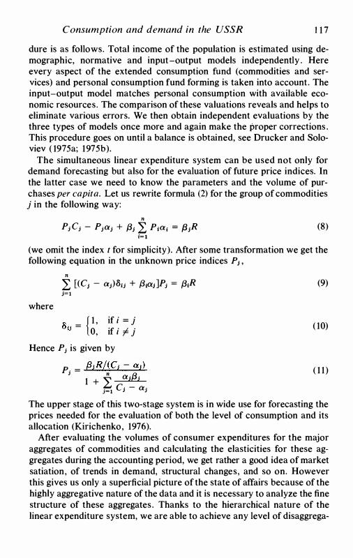
Consumption and demand in the USSR 1 1 7

dure is as follows. Total income of the population is estimated using de­mographic, normative and input-output models independently . Here every aspect of the extended consumption fund (commodities and ser­vices) and personal consumption fund forming is taken into account. The input-output model matches personal consumption with available eco­nomic resources. The comparison of these valuations reveals and helps to eliminate various errors. We then obtain independent evaluations by the three types of models once more and again make the proper corrections . This procedure goes on until a balance is obtained, see Drucker and Solo­viev ( 1975a; 1975b). The simultaneous linear expenditure system can be used not only for

demand forecasting but also for the evaluation of future price indices. In the latter case we need to know the parameters and the volume of pur­chases per capita. Let us rewrite formula (2) for the group of commodities j in the following way:

n Pi Ci - Piai + /3i L P1a1 = f3JR (8)

i=l (we omit the index t for simplicity). After some transformation we get the following equation in the unknown price indices P1 ,

where

n L [(CJ - ai)8ii + {31a1]Pi = {31R j=l

l:>,.1 = {01 ,,

if i = j u if i "l j

Hence Pi is given by

P _ {31R/(C; - a1) j -1 + i a1/3i

j=l cj - aj

(9)

( 10)

( 1 1)

The upper stage of this two-stage system is in wide use for forecasting the prices needed for the evaluation of both the level of consumption and its allocation (Kirichenko, 1976). After evaluating the volumes of consumer expenditures for the major

aggregates of commodities and calculating the elasticities for these ag­gregates during the accounting period, we get rather a good idea of market satiation, of trends in demand, structural changes, and so on. However this gives us only a superficial picture of the state of affairs because of the highly aggregative nature of the data and it is necessary to analyze the fine structure of these aggregates . Thanks to the hierarchical nature of the linear expenditure system, we are able to achieve any level of disaggrega-

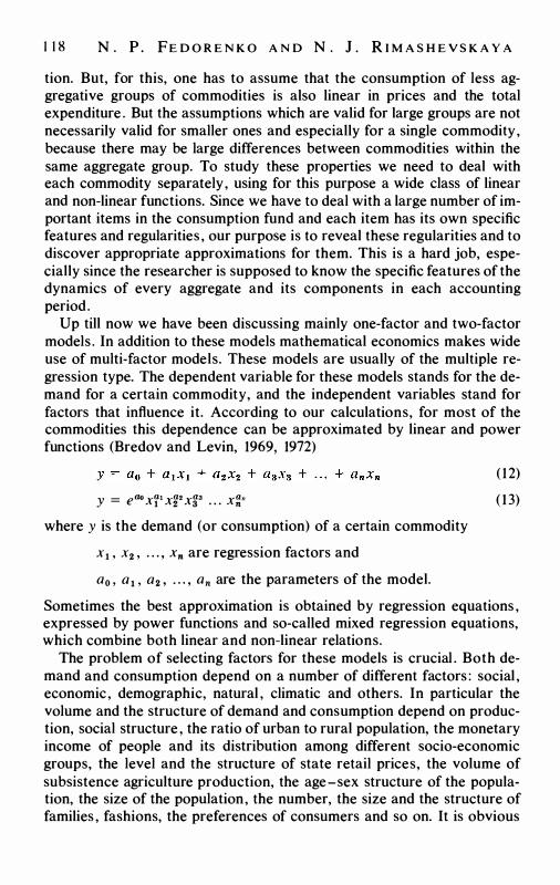
1 1 8 N . P . FE D O R E N K O A N D N . J . R I M A S H E V S K A Y A

tion. But, for this, one has to assume that the consumption of less ag­gregative groups of commodities is also linear in prices and the total expenditure . But the assumptions which are valid for large groups are not necessarily valid for smaller ones and especially for a single commodity, because there may be large differences between commodities within the same aggregate group. To study these properties we need to deal with each commodity separately, using for this purpose a wide class of linear and non-linear functions. Since we have to deal with a large number of im­portant items in the consumption fund and each item has its own specific features and regularities , our purpose is to reveal these regularities and to discover appropriate approximations for them. This is a hard job, espe­cially since the researcher is supposed to know the specific features of the dynamics of every aggregate and its components in each accounting period.

Up till now we have been discussing mainly one-factor and two-factor models . In addition to these models mathematical economics makes wide use of multi-factor models. These models are usually of the multiple re­gression type. The dependent variable for these models stands for the de­mand for a certain commodity, and the independent variables stand for factors that influence it. According to our calculations, for most of the commodities this dependence can be approximated by linear and power functions (Bredov and Levin, 1969, 1972)

y = eao xf' x�• xga . . . X�"

where y is the demand (or consumption) of a certain commodity

x 1 , x2 , • • • , Xn are regression factors and

a0 , a 1 , a2 , • • • , an are the parameters of the model.

( 12)

( 1 3)

Sometimes the best approximation is obtained by regression equations , expressed by power functions and so-called mixed regression equations, which combine both linear and non-linear relations.

The problem of selecting factors for these models is crucial . Both de­mand and consumption depend on a number of different factors : social , economic, demographic, natural , climatic and others. In particular the volume and the structure of demand and consumption depend on produc­tion, social structure , the ratio of urban to rural population, the monetary income of people and its distribution among different socio-economic groups, the level and the structure of state retail prices, the volume of subsistence agriculture production, the age-sex structure of the popula­tion, the size of the population, the number, the size and the structure of families , fashions, the preferences of consumers and so on. It is obvious

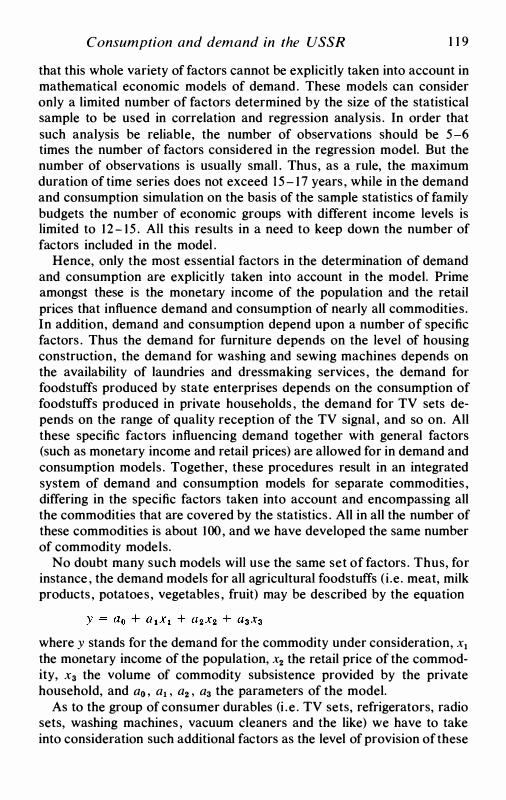
Consumption and demand in the USSR 1 1 9

that this whole variety of factors cannot be explicitly taken into account in mathematical economic models of demand. These models can consider only a limited number of factors determined by the size of the statistical sample to be used in correlation and regression analysis . In order that such analysis be reliable, the number of observations should be 5-6 times the number of factors considered in the regression model. But the number of observations is usually small . Thus, as a rule, the maximum duration of time series does not exceed 15- 1 7 years , while in the demand and consumption simulation on the basis of the sample statistics of family budgets the number of economic groups with different income levels is limited to 1 2- 15 . All this results in a need to keep down the number of factors included in the model .

Hence, only the most essential factors in the determination of demand and consumption are explicitly taken into account in the model. Prime amongst these is the monetary income of the population and the retail prices that influence demand and consumption of nearly all commodities. In addition, demand and consumption depend upon a number of specific factors . Thus the demand for furniture depends on the level of housing construction, the demand for washing and sewing machines depends on the availability of laundries and dressmaking services, the demand for foodstuffs produced by state enterprises depends on the consumption of foodstuffs produced in private households , the demand for TV sets de­pends on the range of quality reception of the TV signal , and so on. All these specific factors influencing demand together with general factors (such as monetary income and retail prices) are allowed for in demand and consumption models . Together, these procedures result in an integrated system of demand and consumption models for separate commodities , differing in the specific factors taken into account and encompassing all the commodities that are covered by the statistics . All in all the number of these commodities is about 100, and we have developed the same number of commodity models.

No doubt many such models will use the same set of factors . Thus, for instance , the demand models for all agricultural foodstuffs (i.e. meat, milk products , potatoes, vegetables , fruit) may be described by the equation

where y stands for the demand for the commodity under consideration, x1

the monetary income of the population, x2 the retail price of the commod­ity, x3 the volume of commodity subsistence provided by the private household, and a0 , a1 , a2 , a3 the parameters of the model.

As to the group of consumer durables (i .e . TV sets, refrigerators, radio sets, washing machines , vacuum cleaners and the like) we have to take into consideration such additional factors as the level of provision of these

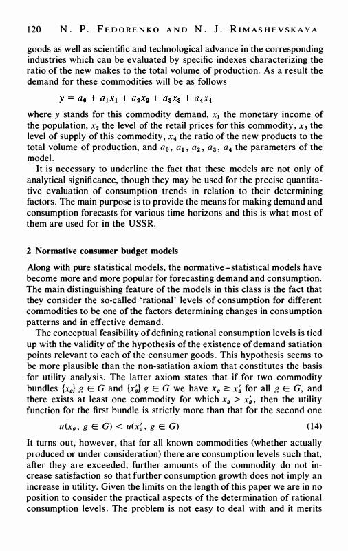
1 20 N . P . F E D O R E N K O A N D N . J . R I M A S H E V S K A Y A

goods as well as scientific and technological advance in the corresponding industries which can be evaluated by specific indexes characterizing the ratio of the new makes to the total volume of production. As a result the demand for these commodities will be as follows

where y stands for this commodity demand, x1 the monetary income of the population, x2 the level of the retail prices for this commodity , x3 the level of supply of this commodity, x4 the ratio of the new products to the total volume of production, and a0 , a1 , a2 , a3 , a4 the parameters of the model .

It is necessary to underline the fact that these models are not only of analytical significance, though they may be used for the precise quantita­tive evaluation of consumption trends in relation to their determining factors . The main purpose is to provide the means for making demand and consumption forecasts for various time horizons and this is what most of them are used for in the USSR.

2 Normative consumer budget models

Along with pure statistical models, the normative-statistical models have become more and more popular for forecasting demand and consumption. The main distinguishing feature of the models in this class is the fact that they consider the so-called 'rational ' levels of consumption for different commodities to be one of the factors determining changes in consumption patterns and in effective demand.

The conceptual feasibility of defining rational consumption levels is tied up with the validity of the hypothesis of the existence of demand satiation points relevant to each of the consumer goods . This hypothesis seems to be more plausible than the non-satiation axiom that constitutes the basis for utility analysis. The latter axiom states that if for two commodity bundles {xu} g E G and {x�} g E G we have Xu � x� for all g E G, and there exists at least one commodity for which Xu > x� , then the utility function for the first bundle is strictly more than that for the second one

u(xg , g E G) < u(x� , g E G) ( 14)

It turns out, however, that for all known commodities (whether actually produced or under consideration) there are consumption levels such that, after they are exceeded, further amounts of the commodity do not in­crease satisfaction so that further consumption growth does not imply an increase in utility. Given the limits on the length of this paper we are in no position to consider the practical aspects of the determination of rational consumption levels . The problem is not easy to deal with and it merits

Consumption and demand in the USSR 1 2 1

special investigation. We would only claim that due to the research in the USSR we possess an approximate procedure for the calculation of con­sumption levels for the most important foodstuffs, textiles, footwear and various durables , which were lately accepted by the planning institutions as the guide for forecasting welfare in the long-term (Sarkisyan and Kuz­nezova, 1967; Maier, 1977). The data on rational consumption levels also provide us with an opportunity to make a closer link between utility anal­ysis and the practical problems of economic and social planning.

Our economists have suggested several approaches to the utilisation of the rational consumption levels while forecasting demand and individual consumption. Let us consider one of them from Lahman and Sokolovs­kaya ( 1978).

The whole set of commodities is divided into 2 groups: the group of cur­rent consumer goods Gr , that includes all foodstuffs, non-durable and semi-durable goods; and the group of durable goods GD that includes the major part of cultural and household goods and some products of light in­dustry . For each of these groups the demand and consumption forecast is made in two stages. First of all, for the current consumer goods Gr we make a forecast of the total per capita expenditure for the group - W r . This forecast i s based on the following idea about the dynamics of expenditure. If the real expenditure for the commodities belonging to Gr is considerably less than the cost of the bundle of these commodities formed in accordance with the rational consumption levels, then the rela­tion between W r and the income volume W is close to linear. As soon as the consumption approaches the rational norms the growth of Wr(W) slows down. And when the expenditure for the group Gr reaches the rational level Wr( Wr = LaEGrx0II) (where x0 stands for the rational con­sumption level for the commodity g 1 II and II is the price of this commod­ity) the further growth of Wr depends only on changes in retail prices II, that take place as a result of the improvements in quality and variety of the commodities and some other factors .

This dependence can be described by the relation

The first equation represents a curve that consists of two separate parts, while the inequalities point out the part essential for our forecast . The parameters A, B and a are chosen in such a way that the Wr(W) function, described implicitly by ( 15), provides the best approximation to the refer­ence period Wr(W) function. Keeping in mind the inequality Wr < Wr we solve the equation and obtain the forecast formula

1 22 N . P . F E D O R E N K O A N D N . J . R I M A S H E V S K A Y A

Taking into account the W r values for the forecast period, we can esti­mate the consumption levels x0 and the per capita expenditure x0Il0 at specific times. Consumer behaviour at each moment t is assumed to be determined by each consumer attempting to maximize his satisfaction of wants for the commodities of group Gr within the constraints of his given expenditure value Wr(t) . That is, at each t we have to solve

max u' (x0g E Gr) = Umax - L (�o (x0 - x)2) with L x0Il0 = Wr(t), x0 � 0 ( 17)

oEG (where the parameter a0 stands for the utility index for the relevant com­modity) . The solution of this problem can be obtained with the help of the Lagrange multiplier approach.

As for durables, the main factor that is to be optimized by the consumer is the per capita supply of each commodity . Hence, the model described above has to be essentially modified. The total volume of purchased dura­bles x0(t) at the moment t consists of two parts. One part is needed to re­place physical depreciation and is equal to M0(t) G0(t) , where M0(t) stands for the depreciation rate. The other part is used to increase the individual (or household) ownership and is equal to ( Y0 (t) - Y0(t - 1 )) . We have

( 18)

To forecast the per capita (per household) purchases of each durable we transform ( 18) into

( 19)

where L(t) stands for the size of the population or the number of house­holds .

Similarly to the nondurable case we introduce an asymptotic function W v (t) that reflects the cost dynamics of the purchased commodities from the Gv group with y0(t) = Yo (where Yo is the rational supply level for the durable consumer goods). Finally we may construct a Wv(t) function cor­responding to the function W v(t) for the reference period at the very beginning of the forecast period and which asymptotically approaches W v at the end of it.

To predict the per capita supply for individual commodities y0(t), the utility functions U can also be used. But for this it should be defined on the set of {y0 (t)}g E Gv . The utility of vector Yo is assumed to reach its maximum when Yo = y. Equating au/ay0 to a0(y0 - min(y0y0)) we have to find y0(t) and x0(t) such that the utility function U reaches its maximum

Consumption and demand in the USSR 1 23

provided

L X0 (t)I10(t) = Wv(l) As to the practical implementation of these models we should acknowl­

edge that the adequacy of the forecast estimates obtained using them de­pends to a large extent upon the validity of the rational consumption levels and the degrees of satisfaction of the latent demand for the com­modities as well as on the reliability and completeness of the information concerning other factors accounted for by the model (i .e. the dynamics of income, prices , life expectancy for durables and so on). Even so, as prac­tice shows, this approach is much more realistic and practical than dealing with unknown and possibly even constructively undefinable utility func­tions .

3 Structural models

Another important direction for consumption studies that has come into being quite recently , deals with the investigation of the consumption ty­pology and the design of structural models (Karapetyan and Rimashevs­kaya, 1977; Aivazyan and Rimashevskaya, 1978). Many investigators have acknowledged the importance and urgency of establishing a con­sumption ' typology' , that is, of detecting comparatively steady and char­acteristic consumption types created under certain conditions of the con­sumer' s life. Until recently they were treated, as a rule, with the help of statistical clustering techniques and correlation - regression analysis. But one can take another point of view and study consumption using mul­tivariate statistical techniques , in particular pattern recognition tech­niques, principal component techniques and others .

Multivariate statistical theory regards multivariate objects as a set of points or vectors in the space of their characteristics . In the consumption area the set of elementary consumer units-households stands for the set of objects to be studied. Each family is characterized on the one hand by a given set of determinants (i .e . factors that determine the household life style) and on the other hand by the set of behavioural parameters re­flecting the real expenditures of a household for various commodities . In studying the consumption typology one can in theory lean upon the fact that the actual consumption structure is the result of free choice by con­sumers and thus satisfies their wants in the best possible way within the budget constraint.

Differences in welfare among the population and corresponding dif­ferences in consumption result from the socialist principle of distribution of the major part of the produced commodities according to the amount of

1 24 N . P . F E D O R E N K O A N D N . J . R I M A S H E V S K A Y A

labour, given that labour is itself distributed unevenly. Households differ also in their demographic composition. In addition, individual features of educational status and working skills, cultural standards , professional training and so on influence the consumption structure of different social groups and strata.

We may distinguish at least three ways that the consumer's life style influences the consumption pattern:

(i) The regional level, which takes into account the economic, natural and climatic particularities of the region;

(ii) The household level, which considers household conditions such as the family income, the quality and the size of the residence, accumu­lated ownership, the age of the family , its size, composition and so on;

(iii) The personal level, which takes into account the age, education and occupation of the consumer. Here we must take into account also such vague and implicit features of the individual as his moral , ethical and psychological norms and aspirations.

To each level of welfare, that is, every combination of objective condi­tions of family activity, there corresponds its own set of wants and prefer­ences that determine the specific nature of consumer behaviour and the actual consumption structure . Hence, families that differ in the conditions of their activity differ in their consumer behaviour as well. And this gives grounds for the belief that such a detection of several steady consumption types is possible. The problem of establishing consumption types can be reduced formally to the research of clusters of points or vectors in the multi-dimensional space of attributes associated with the families under investigation. Each cluster of points corresponds to a certain class and the corresponding families are close in their consumer behaviour. To formal­ize, let {y1} i = 1 , 2, . . . , n be a set of points in the multi-dimensional space of behavioural attributes . We look for some partition of the set S11 into an unknown number N of disjoint classes s�i , s<;> , S�3> , . • . , s';f> .

The study and analysis of the differentiations of consumer behaviour consist of the following stages:

(i) The initial formulation of economic problems, where we determine research objectives and prove the conceptual feasibility of a multi­variate analytical approach;

(ii) The gathering of all the necessary information and preliminary data processing, including its comprehension and its reading into the com­puter;

(iii) The selection of a taxonomy algorithm and the determination of the main types of consumer behaviour through the partitioning of the set of household-points in the space of the chosen consumption attri­butes;

Consumption and demand in the USSR 1 25

(iv) The meaningful analysis of the consumer behaviour within the con­sumption classes so obtained;

(v) The selection of consumption classification factors and the design of the consumer ' images' .

The choice of attributes that gives the best description of the objects under classification is the most important point of the second stage. It is quite natural to take those attributes for which the differentiation of con­sumer expenditures is the greatest. As a result of such a choice the dimen­sion of the attribute space is reduced by neglecting irrelevant information. The reduced number of attributes together with their high information content makes it easier to study the phenomenon and makes the interpre­tation of the results of our taxonomy more straightforward and more meaningful. As to the way we diminish the dimension of the attribute space we have two alternatives. The first consists of the selection of a lim­ited number of attributes from the initial set of given objective features , while the second is the aggregation of characteristics and expenditures. In both cases one may employ both formal and informal techniques for attri­bute selection and aggregation.

In reference to the socio-demographic and economic characteristics of the family it is advisable to consider the level of material welfare (that is the monetary per capita income of the family), the size of the family, the fertility of the family (that is the presence and number of children), the so­cial affiliation of the family , the profession of the head of the family, the size and quality of the dwelling, and the number of durables owned. How­ever, the number of these factors can be extended when available infor­mation permits .

The factors that determine the classification of the family according to consumption type can be considered as type-forming. They play the main role in the formation of the consumption structure, while all other factors determine only random fluctuations within the same type of consumer be­haviour. No doubt the values of the separate type-forming factors vary within every consumption type, that is , they are characterized by some distribution law. Thus it is quite natural to consider as type-forming those factors, whose distribution laws for different consumer behaviour classes differ most of all. In accordance with this principle we have selected the specific attributes contributing to the formation of consumption behaviour classes and as a result constructed a socio-demographic ' image' for each class.

If the size of the sample is not very large, and each household can be re­cognized as a separate entity, the choice of type-forming attributes for each class of consumer behaviour can be performed without resorting to a formal treatment. Instead we obtain the average socio-demographic esti­mates for families in each class and then try to correlate the predominant

1 26 N . P . F E D O R E N K O A N D N . J . R I M A S H E V S K A Y A

structural indices of socio-demographic attributes with the distinguishing features of the consumer behaviour of the given household class . Along with structural indices the analysis also takes into account data on each characteristic distribution within classes as well as intra- and inter-class variability and the correlation between socio-demographic attributes and the indices of consumer behaviour. However, for large sample sizes, formal techniques for consumer image identification are needed; in partic­ular, one may use factor analysis and other taxonomic techniques . After one of these methods has provided us with the division of the total set of attributes into groups, we may regard every such a group as an aggregate . This approach carries through the idea of reducing the number of socio-demographic attributes with minimal loss of information about the sample as a whole.

In studying consumption processes we have to deal with data of a multi­variate nature due to the fact that both the number of registered attributes in each family and the number of objects to be considered are very large. The selection of the most informative attributes among these character­istics is performed by interpreting the variation of these characteristics and their relation to the main consumption-forming factors . At this stage we may take into consideration the a priori conceptions of the inves­tigator about the informative significance of the factors for the differentia­tion of consumption. The aggregation of behavioural characteristics may be based on various principles . Thus, for the aggregation of the expendi­tures on foodstuffs one may lean upon the principle of allocation of lim­ited raw material , while for that on non-foods one may lean upon the prin­ciple of specific wants to be satisfied. This approach has resulted in the reduction of the number of attributes by nearly a factor of 3 - from 100 to 37.

At the second stage of aggregation all the characteristics of consumer behaviour can be reduced to 4 expenditure groups in accordance with the following classification of expenditures: ( 1 ) foodstuffs ; (2) non-foods ; (3) services ; (4) public catering. Together with the choice of informative attri­butes and their aggregation one may also use formal techniques . How­ever, their use meets with difficulties in the economic interpretation of the results . These techniques are only to be advised if the feasibility of con­sumption types classification can be established and the classification can be interpreted. This latter fact may be regarded as a kind of a check for the results obtained by some formal technique of partitioning the attribute space. If two different formal approaches lead to the same partitioning of the attribute space, one may regard this as the confirmation of the validity of the technique, which in turn reduces consumption classification time and provides a unified computer program for the solution of the problem.

Consumption and demand in the USSR 1 27

The classification structure so obtained represents a rather stable system of consumption models for some household types . The consump­tion behaviour of each of these types can be considered constant for the medium-range period (i .e. 7 - 1 0 years). Under such conditions, changes of some factors in the household activity can be viewed as a transition of this household to another type group, while the changes of the consump­tion structure in general can be viewed as an effect of modifications of weight of different types of consumer behaviour within the totality of households . Here we have a forecast based on structural consumption models, while in the present structural model (Karapetyan and Rima­shevskaya, 1977) we take into account only one factor, namely, income; in the structural models based on the consumer taxonomy we account for a series of factors that allow us to adjust the forecast calculations and make them more stable over time. This is an obvious advantage of these models .

The decomposition into consumer groups which are homogeneous in the given set of characteristics also opens the way for the wide use of correlation - regression techniques for analysis and forecasting. The parameters of models based on homogeneous household classification are more reliable and meaningful than those built from a more heteroge­neous set. Thus we bypass one of the most important and unsolved problems of the proper representation of consumption. Combining the classification methods and the correlation techniques we may expect to achieve a good agreement between the results and reality, for current esti­mates as well as for forecasts. The identification of stable types of con­sumers, with each having its own system of values and preferences governing the choice of commodities, opens entirely new vistas for the simulation of normative consumer budgets .

Thus, the studies of consumption and demand in the USSR follow various directions, each aimed at the improvement of planning practice in this country.

References

Aivazyan, S. A. and N. M. Rimashevskaya ( 1972), Consumption Typology: Moscow, N auka.

Bazarov, V. A. ( 1927), ' Use of budget data for urban demand mix elaboration within a perspective general plan' , Planned Economy, p. 5 .

Bredov, V. M. and A. I . Levin ( 1969), 'Economic and mathematical models of de­mand' , Economica (Moscow).

( 1972), 'Forecasting methods' , Economica (Moscow). Drucker, S. G. and J. P. Soloviev ( 1975a), 'Modelling of consumer demand' ,

Economica i Matematicheski Metodi, Vol. II .

1 28 N . P . F E D O RE N K O A N D N . J . R I M A S H E V S K A Y A

(1975b), 'A two-level model for analysis and forecasting of population demand' , Economica i Matematischeski Metodi, Vol. II .

Karapetyan, A. H. and N. M. Rimashevskaya ( 1977), Family Income and Con­sumption Differential Balance: Moscow, Nauka.

Kirichenko, N. ( 1976), 'Rational consumer budgeting in the system of long-term forecasts' , in Problems of Long-Term National Economic Forecasting, Cen­tral Economic Mathematical Institute, Moscow.

Lahman, I. L. and T. A. Sokolovskaya, ( 1978), 'A normative model for fore­casting personal consumption' , Economica i Matematicheski Metodi, Vol. 8.

Maier, V. F. ( 1977), The Living Standard of the Population of the USSR, Moscow, Mis!.

Sarkisyan, G. S. and N. P. Kuznezova ( 1967), ' Family demand and income ' , Economica (Moscow).

Stone , R. ( 1954), 'Linear expenditure systems and demand analysis: an applica­tion to the pattern of British demand' , Economic Journal, Vol. 64, pp. 5 1 1 -27.

Strumilin, S. G. ( 1965), Selected Works, Vol. 5, Moscow, Nauka.

PART TWO

The theory of index numbers

Introduction to part two

The theory and measurement of economic index numbers presents side by side some of the most difficult and abstruse theory with the most immediately practical issues of everyday measurement. The construction of index numbers is an essential part of all social accounting; without compression and aggregation the mass of quantities and prices thrown up by the economic system would be incomprehensible . Yet from the outset such aggregation has been known to be meaningful only in the context of welfare measurement. But to what extent are welfare-based index numbers practical? In his book on index numbers [56] written for the OEEC (now OECD), Sir Richard Stone addressed the question of whether practical international standards for index number construction could be established in line with his earlier standardized system of national accounts. Sir Richard gives the following reasons why the welfare ap­proach is useful:

First , they give content to such concepts as real consumption which might other­wise be vague and obscure ; second, they bring out the fundamental difficulties in establishing empirical correlates to concepts such as real consumption and so help to show what can and what cannot usefully be attempted in the present state of knowledge ; finally they show the circumstances in which particular empirical cor­relates, such as a measure of real consumption which can actually be constructed, are likely to provide a good or a bad approximation to the concepts of the theory. ([56], pp. 18-19)

Much of the material in this section is an elaboration of these three points. Although index number theory is at least as old as consumer theory it­

self, it has been a somewhat neglected area at least until the last few years . However, the world-wide increase in inflation rates over the last decade accompanied by rapid changes in relative prices has caused a re­cent upsurge of interest in both theory and measurement. When relative prices show large changes, it makes a great difference exactly how price index numbers are constructed. At the same time, the fact that different consumers consume different bundles of goods means that the index number which measures one family' s welfare may be quite misleading if applied to another. Poor families have different price indices from rich families, families with children differ from those without, old families

1 30

Introduction 1 3 1

from young families, and so on. These differences were well understood in Cambridge in the 1950s (see in particular Prais, 1959) and have certainly been empirically important in recent times both in Britain and the United States (see, for example, Deaton and Muellbauer, 1980, chapter 7, for some evidence and further references).

In this section, however, it is the theory which is highlighted. In the first chapter, that by Sydney Afriat, the question at issue is whether it is conceptually possible to construct a price index from a given set of obser­vations on prices and quantities . If price indices are to be based on wel­fare, welfare itself must be well-defined and we can do this only from data which are consistent with rational behaviour. For example, if we have two periods with price vectors p0, p1 and quantities q0 and q1 , then if p0

• q0 > p0 • q1 we know that, in situation 0, q1 could have been chosen

but was not. Hence if we also find that p1 • q1 > p1

• q0, behaviour is not consistent with rationality, no utility function exists and a price index cannot be constructed . Afriat goes further than this and insists that the existence of a preference ordering by itself is not sufficient for the exis­tence of the price index. If this latter is to be unique and unambiguous, it cannot vary from individual to individual and this will occur only if de­mand patterns in terms of budget shares are the same for everyone. As Afriat has shown elsewhere (e.g. Afriat, 1977), two observations will allow the construction of a utility function consistent with such behaviour if and only if p1

• q1 / p0 • q1 ::5 p1

• q0 / p0 • q0, that is if the Paasche price

index is no greater than the Laspeyres price index, a condition which also rules out the possibility of the earlier contradiction. The question of how this analysis extends to many observations is the subject of the pres­ent paper. In it, Afriat defines generalized Paasche and Laspeyres indices which allow an extension of the theorem; he also presents an algorithm for calculating the relevant quantities so that his results can be applied straightforwardly to any finite set of data.

The second chapter in the section is an extremely comprehensive and clear survey of the whole area of economic index numbers by Erwin Diewert. Basing his analysis on modern duality theory, he provides an in­tegrated treatment of index numbers encompassing not only consumer be­haviour but also the theory of the firm. The cost or expenditure function is used to derive the Koniis or ' true' cost-of-living index number and the conventional bounds theorems proved. The dual quantity index numbers due originally to Malmquist ( 1953) are also fully discussed as is their rela­tionship to the Koniis price indices. The duality framework renders the results easily proved and provides a straightforward way of understanding how the various concepts relate to one another. In the final sections of the paper, Diewert shows how particular well-known index number formulae, for example Fisher's ' ideal' index, can be derived from specific prefer-

1 32 T H E O RY O F I N D E X N U M B E RS

ence structures. Perhaps the most interesting of these theorems shows that the Tornqvist logarithmic price index number, in which the logarithmic price relatives are weighted by the average of the two periods' budget shares, can be justified exactly in terms of a specific but flexible formation of preferences. Such theorems take us a long way towards an integration of theory and practice.

References for introduction to part two

Afriat, S. N. ( 1977), The price index, Cambridge University Press, New York. Deaton, A. S . and J. Muellbauer ( 1980) , Economics and consumer behavior, Cam-

bridge University Press, New York. Malmquist, S. ( 1953), ' Index numbers and indifference surfaces' , Tradajos de Es­

tadistica, 4, pp . 209-41 . Prais, S . J . ( 1959), 'Whose cost of living?' , Review of Economic Studies, 26,

pp. 126-34.

6 On the constructability of consistent

price indices between several periods simultaneously1

S . N . A F R I AT

Introduction

A price index refers to a pair of consumption periods, and price-index for­mulae usually involve demand data from the reference periods alone. When there are many periods, a price index can be determined from any one period to any other, in each case using the data from just those two periods . But then consistency questions arise for the set of price indices so obtained. Especially, they must have the consistency that would follow from their being ratios of 'price levels' . The well-known tests of Irving Fisher have their origin in such questions . When these tests are regarded as giving identities to be satisfied by a standard formula and are taken in combination, it is impossible to satisfy them. Such impossibility remains even with partial combinations. Eichhorn and Voeller ( 1 976) have given a full account of the inconsistencies between Fisher's tests . Reference is made there for their results and for the history of the matter.

Fisher recognizes the consistency question also in his idea of the 'recti­fication of pair comparisons' . In this the price indices are all calculated, as usual, separately and regardless of any consistency they should have together, and then they are all adjusted in some manner so that they can form a consistent set. For instance , by 'crossing' a formula with its 'an­tithesis' you got one that satisfied the 'reversal' test. Here he takes one of the tests separately as if any one could mean anything on its own, and contrives a formula to satisfy it. This is how he arrived at his ' ideal' index. It is ' ideal' because it satisfies the 'reversal' test but not so when those other tests are brought in. The search for a really ideal index seemed a hopeless task.

In any case these tests are just negative criteria for index-number­making, showing how a formula can be rejected and telling nothing of how one should be arrived at . Something is to be measured and it is not yet

1 Support of this work by the National Research Council of Canada is acknowledged with thanks.

1 3 3

1 34 S . N . A F R I AT

considered what, but whatever it is it must fit a certain mould. Here is not measurement but a ritual with form. In the background thought, what is to be measured is the price level, though prices are many so no one quite knows what that means, and a price index is a ratio of price levels . There­fore the set m2 price indices Pr8 (r, s = 1 , . . . , m) between m periods 1 , . . . , m must at least have the consistency required by their being ratios Prs = P8/Pr of m 'price levels' Pr(r = 1 , . . . , m). Therefore Prr = 1 , Prs = P;.1 , PrsPst = Prt and so forth. There are other parts to Fisher' s tests and here we have the part that touches just the ratio aspect.

In a seemingly more coherent approach, utility makes the base for what is being measured. There would be no problem there at all if only the util­ity function or order to be used could be known. But it is not known and therefore it is dealt with hypothetically. Its existence is entertained and inferences are made from that position. With utility in the picture the nat­ural object of measurement is the 'cost of living' , and at first we know nothing of the price-level or of a price-index. Giving intelligibility to the price index in the utility framework involves imposing a special restriction on utility.

Let M 0 be any income in a period 0 when the prices are given by a vector Po . Hypothetically , the bundle of goods x0 consumed with this in­come has the highest utility among all those which might have been con­sumed instead . Then it is asked what income M, in a period 1 when the prices are p1 provides the standard of living, or utility , attained with the income M0 in period 0. With p0 , p1 fixed and the utility order given, M1 is determined as a function M1 = F10(M0) of M0 , where the function F10 de­pends on the prices p0 , p1 and the utility order. Without making any for­bidding extra assumptions it can be allowed that this is a continuous increasing function, and that is all. However, turning to practice with price-indices, we find that to offer a relationship between M 0 and M1 is the typical use given to a price index . The relationship in this case has the form M1 = P10M0 , P10 being the price index . In other words, using a price-index corresponds to the idea that there is a homogeneous linear re­lation between M 0 , M 1 or that the relation is a line through the origin, the price-index being the slope.

To give the function F10 , just this form has implications about the utility from which it is derived. That utility must have a conical structure that is a counterpart of linear homogeneity of that function: if any commodity bundle x has at least the utility of another y then the same holds when x

and y are replaced by their multiples xt and yt by any positive number t. To talk about a price-index and at the same time about utility, this as­sumption about the utility must be made outright.

If a conical utility is given, relative to it a price-index P 10 can be com-

Constructability of consistent price indices 1 35

puted for any prices p0 , p1 • Then, as explained further in section 1 1 , it has the form P10 = Pi/Po where P0 = fJ(p0), P1 = fJ(p1 ) are the values of a concave conical function (J depending on prices alone. Price indices so computed for many periods automatically satisfy various tests of Fisher. The issue about those tests therefore becomes empty in this context, and pair-comparisons so obtained need no 'rectification' . But a remaining issue comes from the circumstance that a utility usually is not given. Should one be proposed arbitrarily as a basis for constructing price indi­ces, there can be no objection to it merely on the basis of the tests, at least with those that concern the ratio-aspect of price indices.

With each price-index formula P10 of the very many he surveyed, Fisher associated a quantity-index formula X10 in such a way that the product is the ratio of consumption expenditures M0 = p0xo , M1 = p1x1 in the two periods . For instance with the Laspeyres price index P10 = p1x0/p0x0 , the corresponding quantity-index is X10 = p1xi/p1x0 , and then

P10X10 = (P1Xo/P0Xo)(P1Xi/P1Xo) = P1Xi/P0Xo = Mi/Mo As a possible sense to this scheme, it is as if, beside the price-index being a ratio Pio = Pi/Po of price-levels, also the quantity-index is a ratio X10 = Xif Xo of quantity levels, and price-level multiplied with quantity level is the same as price-vector multiplied with quantity-vector, that is

PoXo = PoXo = Mo , P1X1 = P 1X1 = Mi to give

P10X10 = (Pi/Po)(Xi/Xo) = (P1X1 )/(P0Xo) = Mi/Mo Here there is the simple result that all prices are effectively summarized by a single number and all quantities by a single quantity number, and in­stead of doing accounts by dealing with each price and quantity sepa­rately, and also with their product that gives the cost of the quantity at the price, the entire account can be carried on just as well in terms of these two summary price and quantity numbers , or levels, whose product is, miraculously, the cost of that quantity level at that price level. Though there are many goods and so-many prices and quantities, still it is just as if there was effectively just one good with a price and obtainable in any quantity at a cost which is simply, as with a simple goods, the product of price times quantity. Any mystery about the meaning of a price index van­ishes, because it becomes simply a price . Were this scheme valid we could ask for so much utility, enquire the price and pay the right amount by the usual multiplication. When applied to income M0 in period 0 when the price level is P0 , the level of utility it purchases is X0 = M0/ P0 .

1 36 s . N . A F R I A T

Then the income that purchases the same level of utility in period 1 when the price level is Pi is given by Mi = PiX0 • Hence, by division, Mi/M0 = Pi/Po = P10 , giving the relation Mi = P10M0 as usual.

Whether or not this scheme has serious plausibilities , it is implicit whenever a price index based on utility is in view. However, though such a scheme has here been imputed as belonging to Fisher's system, or con­jured up as though that seems to belong to it or at least gives it an intelligi­bility , it cannot be considered to have clear presence there . For Fisher's system does not have a basis in utility and this scheme does. While this circumstance is not evidence of a union it still might not seem to force a separation. However, a symptom of a decided separation is that, even when many periods are involved, Fisher still followed standard custom in regarding an index formula as one involving the demand data just from its pair of reference periods , and really his system is about such formulae. Then he worried about the incoherence of the set of price indices for many periods so obtained. The utility formulation cares nothing about the form of the formula. When many periods are involved and all the price indices between them are to be calculated, the calculation of one and all should involve the data for all periods simultaneously. In the utility approach immediate thought is not of the demand data and of formulae in these at all , but rather it is of the utility order which gives the basis of the calcula­tions, and necessarily gives coherent results . Instead, Fisher forces inco­herence by rigidly following the standard idea of what constitutes an index formula. The main issue with the utility approach is about the utility function or order. When that utility is settled all that remains to be dealt with is a well-defined objective of calculation based on that utility. The role of the demand data is just to put constraints on the permitted utility order, and consequently price indices based on utility become based on that data. Having such constraints, the first question then is about the existence of a utility order that satisfies them. If none exists then no price indices exist and there the matter ends. Though that is so in the present treatment, by making the constraints more tolerant it is possible to go fur­ther (see Afriat, 1972b and 1973).

In the standard model of the consumer, choice is governed by utility, to the effect that any bundle of goods consumed has greater utility than any other attainable with the same income at the prevailing prices. With this model , the obvious constraint on a utility for it to be permitted by given data is, firstly, that it validate the model for the consumer on the evi­dences provided by that data. Then further, since price-indices are to be dealt with, the conical property of utility should be required.

With this method of constraint and the other definitions that have been outlined, everything is available for developing the questions that are in view. But first there will be a change in formulation that has advantages .

Constructability of consistent price indices 1 37

Instead of requiring that a chosen bundle of goods be represented as being the unique best among all those attainable for no greater cost at the pre­vailing prices, or as being definitely better than any others in utility , it will be required that it be just one among the possibly many best, or one at as least as good as any other. This alters nothing if certain prior assumptions are made about the utility order, for instance that it is representable by an increasing strictly quasiconcave utility function. With the latter assump­tion a utility maximum under a budget constraint must in any case be a unique maximum, and so adding that the maximum is unique just makes a redundance . But we do not want to introduce additional assumptions about utility . A utility is wanted that fits the data in a certain way, and if all that is now wanted in such a fit is that some commodity bundles be re­presented as having at least the utility of certain others then we can always count on a utility function that is constant everywhere to do that service. In making what could at first seem a slight change in the original formulation of the constraint on permitted utilities, the result is no con­straint at all: whatever the data there always exists a permitted utility, for instance the one mentioned which will give zero as the cost of attaining any given standard of living. That change is drastic and no such change is sought. All that is in view is a change that alters nothing important in the results, the effect being something like replacing an open interval by a closed one, while it is better to work with and in any case is conceptually fitting. One possibility is to add a monotonicity condition as an assump­tion about utility expressing that 'more is better' . But, as said, we do not want any such prior assumptions. Instead consider again the original strict condition, that the chosen bundle be the unique best attainable at no greater cost. It implies the considered weaker condition in which the uniqueness has been dropped. But also it implies a second condition: the cost of the bundle is the minimum cost for obtaining a bundle that is as good as it. These two conditions are generally independent, even though relations between them can be produced from prior assumptions about utility, of which we have none, and their combination is implied by the stricter and analytically more cumbersome original condition.

They are just what is wanted. They have equal warrant as economic principles. In the context of cost - benefit analysis they are familiar as constituting the two main criteria about a project, that it be cost-effective or gives best value for the cost, and cost-efficient or the same value is un­attainable at lower cost.

Now the wanted constraint on an admissible utility can be stated by the requirement that every bundle of goods given in the demand data be re­presented by it as cost-effective and cost-efficient. Such a utility can be said to be compatible with the demand data. Then the data is consistent if there exists a compatible utility . It is homogeneously consistent if there

1 3 8 S . N . AF R I A T

exists a compatible utility that moreover has the property of being con­ical , or homogeneous, required whenever dealing with price-indices . A compatible price-index, or a 'true' one, is one derived on the basis of a homogeneous utility that is compatible with the given data.

The first problem therefore is to find a test for the homogeneous consis­tency of the data. In the case where there are just two periods, the test found reduces to a relation that is quite familiar, in a context where it is not at all connected with this test but is offered as a ' theorem' , though cer­tainly it is not that. The relation is simply that the Paasche index from one period to the other does not exceed that of Laspeyres. The relation is symmetrical between the data in the two periods, and so there is no need to put it in this unsymmetrical form where one period is distinguished as the base. But this is the form in which it is familiar and known as the ' Index-Number Theorem' . That the 'Theorem' , or relation, is necessary and sufficient for homogeneous consistency of the demands in the two periods is a theorem in the ordinary sense . It is going to be generalized for any number of periods.

Related to the Index-Number Theorem is the proposition that the Las­peyres and Paasche indices are upper and lower ' limits' for the ' true index' . From the foregoing consistency considerations it is recognized that even the existence of a price index , at least in the sense entertained here, can be contradicted by the data, so certainly some additional qualifi­cation is needed in the ' limits' proposition. Also, what makes an index ' true' has obscurities in early literature. An interpretation emerging in later discussions is that a true index is simply one derived on the basis of utility . This could be accepted to mean one that, in present terms, is com­patible with the given demand data.

With demand data given for any number of periods and satisfying the homogeneous consistency test, a price index compatible with those data can be constructed from any period to any other. It has many possible val­ues corresponding to the generally many compatible homogeneous util­ities. These values describe a closed interval whose endpoints are given by certain formulae in the given demand data.

A special case of this result applies to the situation usually assumed in index-number discussions. In this, the only data involved in a price-index construction between two periods are the data from the two reference periods themselves. For this case the formulae for the endpoints of the in­terval of values for the price index reduce to the Paasche and Laspeyres formulae. Here therefore is a generalization of those well-known for­mulae for when demand data from any number of periods can be per­mitted to enter the calculation of a price-index between any two. The val­ues of these generalized Paasche and Laspeyres formulae are well defined just in the case of homogeneous consistency of the data, under which con-

Constructability of consistent price indices 1 39

dition they have the price-index significance just stated. Then a counter­part of the ' Index-Number Theorem' condition in the context of many periods is that the generalized Paasche formula does not exceed the gen­eralized Laspeyres formula. There seems to be one such condition for each ordered pair of periods, making a collection of conditions . However, all are redundant because they are automatically satisfied whenever the formulae have well-defined values, as they do just in the case of homoge­neous consistency of the data.

For price-indices Prs between many periods to be consistent they should have the form P rs = Ps/ Pr for some Pr . Let P rs , p rs be the generalized Laspeyres and Paasche formulae. These, when they have well-defined values, are connected by the relation Pr.Psr = 1 and have the properties PrsPst ::5 Prt , Pr.Psi ::5 Prt . Then it is possible to solve the system of simul­taneous inequalities Prs 2: P8/ Pr for the Pr . The system Prs ::5 P./ Pr is identical with this, so solutions automatically satisfy

Prs ::5 P8/ Pr ::5 Prs Now it is possible to describe all the price-indices Prs between periods that are compatible with the data and form a consistent set: they are ex­actly those having the form Prs = P8/ Pr where Pr is any solution of the above system of inequalities. The condition for their existence is just the homogeneous consistency of the data. For any solution Pr there exists a homogeneous utility compatible with the data on the basis of which Prs = P8/ Pr is the price-index from period r to period s . This will be shown by actual construction of such a utility .

Now to be remarked is the extension property of any given price­indices for a subset of the periods that are compatible with the data and together are consistent: it is always possible to determine further price indices involving all the other periods so that the collection price-indices so obtained between all periods are both compatible with the data and together are consistent. There is an ambiguity here about a set of price indices being compatible with the data: they could be that with each taken separately , or in another stricter sense where they are taken simulta­neously together. But in the conjunction with consistency the ambiguity loses effect. For price-indices Prs that are all independently compatible with the data, the compatibility of each one with the data being estab­lished by means of a possibly different utility, if they are all consistent there also they are jointly compatible in that also there exists a single util­ity, homogeneous and compatible with the data, that establishes their compatibility with the data simultaneously.

This completes a description of the main concepts and results dealt with in this paper. Further remarks concern computation of the m x m - matrix of generalized Laspeyres indices Pr. , and hence also the gen-

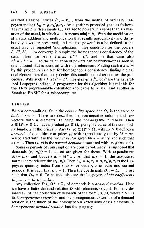
1 40 S . N . A F R I AT

eralized Paasche indices P rs = P;/, from the matrix of ordinary Las­peyres indices Lrs = PsXr/PrXr · An algorithm proposed goes as follows. The matrix L with elements Lrs is raised to powers in a sense that is a vari­ation of the usual, in which a + b means min[ a, b ] . With the modification of matrix addition and multiplication that results associativity and distri­butivity laws are preserved, and matrix 'powers' can be defined in the usual way by repeated 'multiplication' . The condition for the powers L, L2, L3, . . . to converge is simply the homogeneous consistency of the data. Then for some k :5 m, Lk-i = Lk, and in that case also L k = L k+i = . . . so the calculation of powers can be broken-off as soon as one is found that is identical with its predecessor. Finding such a k :5 m by this procedure is a test for homogeneous consistency; finding a diag­onal element less than unity denies this condition and terminates the pro­cedure. With such a k let P = Lk. The elements Prs of P are the general­ized Laspeyres indices . A programme for this algorithm is available for the TI-59 programmable calculator applicable to m :5 6, and another in Standard BASIC for a microcomputer.

1 Demand

With n commodities, fln is the commodity space and fln is the price or budget space. These are described by non-negative column and row vectors with n elements , fl being the non-negative numbers. Then x E fln, p E fln have a product px E fl, giving the value of the commod­ity bundle x at the prices p. Any (x, p) E fln x fln with px > 0 defines a demand, of quantities x at prices p, with expenditure given by M = px. Associated with it is the budget vector given by u = M-1p and such that ux = 1 . Then (x, u) is the normal demand associated with (x, p)(px > 0).

Some m periods of consumption are considered, and it is supposed that demands (xi . Pt)(t = 1 , . . . , m) are given for these. With expenditures Mt = PtXt and budgets Ut = Ml1 Pt , so that UtXt = 1 , the associated normal demands are the (Xt , Ut). Then Lrs = UrXs = PrXs/PrXr is the Las­peyres quantity index from r to s, or with r, s as base and current periods . It is such that Lrr = 1 . Then the coefficients Drs = Lrs - 1 are such that Drr = 0. To be used also are the Laspeyres chain-coefficients LriJ . . . ks = LnL1; . . . Lks ·

Any collection D k fln x fln of demands is a demand relation. Here we have a finite demand relation D with elements (xt , Pt) . For any de­mand (x, p), the collection of demands of the form (xt, p) , where t > 0 is its homogeneous extension, and the homogeneous extension of a demand relation is the union of the homogeneous extensions of its elements. A homogeneous demand relation has the property

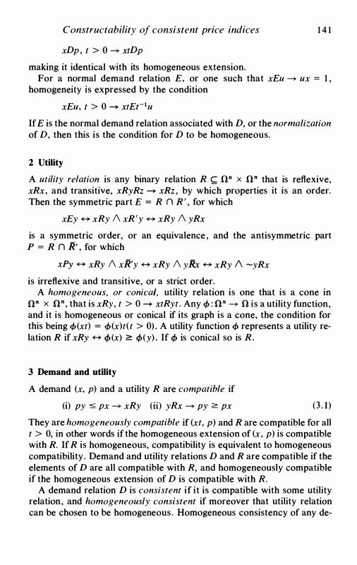
Constructability of consistent price indices 1 4 1

xDp, t > 0 - xtDp

making it identical with its homogeneous extension. For a normal demand relation E, or one such that xEu - ux = 1 ,

homogeneity is expressed by the condition

xEu, t > 0 - xtEr1u

If E is the normal demand relation associated with D, or the normalization of D, then this is the condition for D to be homogeneous.

2 Utility

A utility relation is any binary relation R � on x on that is reflexive, xRx, and transitive, xRyRz - xRz , by which properties it is an order. Then the symmetric part E = R n R ' , for which

xEy � xRy /\ xR'y � xRy /\ yRx

is a symmetric order, or an equivalence , and the antisymmetric part P = R n R' , for which

xPy � xRy /\ xR'y � xRy /\ yRx � xRy /\ -yRx

is irreflexive and transitive, or a strict order. A homogeneous, or conical, utility relation is one that is a cone in

on x On, that is xRy, t > 0 - xtRyt. Any cf> : On - 0 is a utility function, and it is homogeneous or conical if its graph is a cone, the condition for this being cf>(xt) = cf>(x)t(t > 0) . A utility function cf> represents a utility re­lation R if xRy � <f>(x) ;:::: <f>(y) . If <f> is conical so is R .

3 Demand and utility

A demand (x, p) and a utility R are compatible if

(i) py s; px - xRy (ii) yRx - py ;:::: px (3 . 1)

They are homogeneously compatible if (xt, p) and R are compatible for all t > 0, in other words if the homogeneous extension of (x, p) is compatible with R. If R is homogeneous, compatibility is equivalent to homogeneous compatibility . Demand and utility relations D and R are compatible if the elements of D are all compatible with R, and homogeneously compatible if the homogeneous extension of D is compatible with R.

A demand relation D is consistent if it is compatible with some utility relation, and homogeneously consistent if moreover that utility relation can be chosen to be homogeneous. Homogeneous consistency of any de-

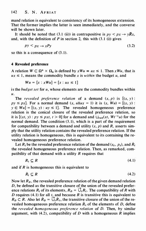
1 42 S . N . A F R I AT

mand relation is equivalent to consistency of its homogeneous extension. That the former implies the latter is seen immediately, and the converse will be shown later.

It should be noted that (3. 1 (ii)) in contrapositive is py < px � yRx, and, with the definition of P in section 2, this with (3 . 1 (i)) gives

PY < px � xPy

so this is a consequence of (3 . 1 ) .

4 Revealed preference

(3 .2)

A relation W c on x On is defined by xWu = ux :::;; 1 . Then xWu, that is ux :::;; 1 , means the commodity bundle x is within the budget u, and

Wu = [x : xWu] = [x : ux :::;; 1 ]

i s the budget set for u, whose elements are the commodity bundles within u .

The revealed preference relation of a demand (x, p) i s [(x, y ) : py :::;; px]. For a normal demand (x, u)(ux = 1 ) it is (x, Wu) = [(x, y) : y E Wu] = [(x, y) : uy :::;; 1 ] . The revealed homogeneous preference relation is the conical closure of the revealed preference relation, so it is [(xt, y) : py :::;; pxt, t > OJ for a demand and Ut>o(xt, Wt-1u) for the normal demand. The condition (3 . 1) , which is a part of the requirement for compatibility between a demand and utility (x, p) and R, asserts sim­ply that the utility relation contains the revealed preference relation. If the utility relation is homogeneous , this is equivalent to its containing the re­vealed homogeneous preference relation.

Let R, be the revealed preference relation of the demand (x, , p,), and R, the revealed homogeneous preference relation. Then, as remarked, com­patibility of that demand with a utility R requires that

R, k R

and if R is homogeneous this is equivalent to

R, k R

(4. 1 )

(4.2)

Now let R0 , the revealed preference relation of the given demand relation D, be defined as the transitive closure of the union of the revealed prefer­ence relations R1 of its elements , R0 = U1R1 • The compatibility of R with D requires ( 4. 1 ) for all t, and because R is transitive this is equivalent to R0 c R. Also let R0 = U1Ri . the transitive closure of the union of the re­vealed homogeneous preference relation R.1 of the elements of D, define the revealed homogeneous preference relation of D. Then, by similar argument, with (4.2), compatibility of D with a homogeneous R implies

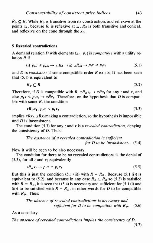
Constructability of consistent price indices 1 43

RD !: R. While RD is transitive from its construction, and reflexive at the points x, , because R, is reflexive at x, , RD is both transitive and conical , and reflexive on the cone through the x1 •

5 Revealed contradictions

A demand relation D with elements (xr , Pr) is compatible with a utility re­lation R if

(i) p,x s; PtXt � x1Rx (ii) xRxt � PtX :2: PtXt (5. 1 )

and D i s consistent if some compatible order R exists. It has been seen that (5. 1 ) is equivalent to

(5 .2)

Therefore, if D is compatible with R, xRDxt � xRx, for any t and x, and also p,x < p1x1 � xRx1 . Therefore, on the hypothesis that D is compati­ble with some R, the condition

(5.3)

implies xRx1 , xRx1 making a contradiction, so the hypothesis is impossible and D is inconsistent.

The condition (5.3) for any t and x is a revealed contradiction, denying the consistency of D. Thus:

The existence of a revealed contradiction is sufficient for D to be inconsistent. (5 .4)

Now it will be seen to be also necessary . The condition for there to be no revealed contradictions is the denial of

(5.3), for all t and x; equivalently

(5.5)

But this is just the condition (5 . 1 (ii)) with R = RD . Because (5. 1 (i)) is equivalent to (5 .2), and because in any case RD !: RD so (5.2) is satisfied with R = RD , it is seen that (5.4) is necessary and sufficient for (5. 1 (i) and (ii)) to be satisfied with R = RD , in other words for D to be compatible with RD . Thus:

The absence of revealed contradictions is necessary and sufficient for D to be compatible with RD . (5.6)

As a corollary:

The absence of revealed contradictions implies the consistency of D. (5.7)

1 44 S . N . A F RI A T

For consistency means the existence of some compatible order, and by (5.5) under this hypothesis RD is one such order. Now with (5 .5) :

The absence of revealed contradictions is necessary and sufficient for the consistency of D and implies

compatibility with RD . (5.8)

By exactly similar argument, xRDx18 and PrX < PrXr8, for any r, x and () > 0, make a homogeneously revealed contradiction denying the homo­geneous consistency of D, or the existence of a compatible homogeneous utility . Then xRDx18 - PrX 2= PrXr8 for all r, x and () > 0 asserts the ab­sence of homogeneously revealed contradictions. Then there is the fol­lowing:

Theorem . For a demand relation to be compatible with some homoge­neous utility relation , and so homogeneously consistent, it is necessary and sufficient that its revealed homogenous preference relation be one such relation, and for this the absence of homogeneously revealed con­tradictions is necessary and sufficient.

This theorem holds unconditionally, regardless of whether or not D is finite . However, when D is finite the homogeneous consistency condition has a finite test, developed in the next two sections.

Because the revealed preference relation of the homogeneous exten­sion of a demand relation is identical with its revealed homogeneous pref­erence relation, it appears now, as remarked in section 3 , that homoge­neous consistency of a demand relation is equivalent to consistency of its homogeneous extension . For, as just seen, the first stated condition on D is equivalent to compatibility with RD and the second with Rv , so this con­clusion follows from RD = Rv .

6 Consistency

Though RD , RD and the Lrs which give the base for the following work are derived from D, they are also derivable from the normal demand relation E derived from D. Therefore there would be no loss in generality if only normal demand relations were considered.

As a preliminary, the definition of the revealed homogeneous prefer­ence relation RD will be put in a more explicit form. This requires identifi­cation of the transitive closure of any relation R with its chain-extension R. An R-chain is any sequence of elements x, y, . . . , z in which each has the relation R to its successor, that is xRyR . . . Rz. Then the chain­extension R is the relation that holds between extremities of R-chains , so xRz = (Vy, . . . )xRyR . . . Rz . The relation R so defined can be identified with the transitive closure of R, that is as the smallest transitive relation containing R, it being such that it is transitive, contains R and is contained

Constructability of consistent price indices 145

in every transitive relation that contains R. Therefore xRvY means x, y are extremities of a chain in the relation U1R1 • This means there exist r, i, . . . , k and z1 , • • . , zk such that xRrz1R1 . . . zkRkY· But, considering the form of the elements of the R, , now we must have Xr = XrOr , z 1 = x101 , . . . , zk = xk Ok for some Or , O; , . . . , Ok > 0, and uky :s; Ok · Accord­ingly, the condition xRvxsOs � UsX � Os for all x, s and Os > 0, for the absence of homogeneously revealed contradictions , can be restated as the condition

(6. 1)

for all r, i , . . . , k, s and Or , 01 , . . . , Ok , 08 > 0. From the form of the ele­ments of the R., , that is

or, in terms of the Laspeyres coefficients ,

Lr1 :s; Or/ O; ' . . . , Lks :s; Ok/ Os � Lsr � Os/ Or

Another way of stating this condition is that

(Lr; , . . . , Lks , Lsr) :s; (Or/O; , . . . , Ok/Os , Os/Or)

(6.2)

(6.3)

is impossible for all r, i, . . . , k, s and Or , 01 , • • • , Ok , Os > 0. This condition will be denoted k.

While theory based on homogeneity is here the main object, in the background is the further theory without that restriction. Some account of that is given here, but it is mainly given elsewhere as already indicated. The dots used in the notation are to distinguish features in this homoge­neous theory from their counterparts without homogeneity. The homoge­neous theory is required in dealing with price indices , but still it has its source in the more general theory. It is useful in this section and later to bring counterparts of the two theories together for recognition of the con­nections and the differences.

Condition (6. 1 ) has been identified with the condition for the absence of homogeneously revealed contradictions that in the last section was shown necessary and sufficient for the consistency of the given demands , that is, for the existence of a homogeneous utility compatible with them all simul­taneously . The weaker condition that is the counterpart without homoge­neity, put in a form that assists comparison, is the condition K given by

(6.4)

is impossible for all r, i, . . . , k, s. By taking the Os all unity in (6. 3) , (6.4) is obtained, so (6. 3) implies (6.4) as should be expected.

If compatibility between demand and utility is replaced by strict com­patibility, by replacing cost-efficacy or cost-efficiency by their strict coun-

1 46 S . N . A F R I A T

terparts , which conditions in fact are equivalent to each other, and strict consistency of any demands means the existence of a strictly compatible utility , then the test for this condition which is a counterpart of (6.4) is the condition K* given by

(6.5) is impossible for all r, i, . . . , k, s unless Xr = X; = = xk = X8 , in which case the equality holds . This is just a way of stating the condition of Houthakker ( 1950), known as the Strong Axiom of Revealed Preference, for when that condition is applied to a finite set of demands instead of to the infinite set associated with a demand function. Here the finiteness is not essential and is just a matter of notation, though in later results it does have an essential part. Corresponding to the results obtained for the less strict consistency, and for homogeneous consistency, as in the Theorem of section 5, Houthakker' s condition is necessary and sufficient for the existence of strictly compatible utility, and for the revealed preference re­lation to be one such utility.

While (6.5) is the ' strict' counterpart of (6.4) , the corresponding coun­terpart for (6.3) is the condition K given by

(6.6)

is impossible for all r, i, . . . , k, s and 6r , 61 , • • • , (Jk , 68 > 0 unless Xr6r =

x1(J1 = . . . = x868 in which case the equality holds . Just as a dot signifies a condition associated with homogeneity, a star

signifies belonging to the ' strict' theory . The various conditions that have been stated have the relations

k - K i i K* - K*

The main result of this section, which is about k in (6.3) being a consis­tency condition, will be part of a theorem in the next section where it is developed into another form.

It can be noted that (6.3) is equivalent to the same condition with r, i, . . . , k, s restricted to be all distinct. For the second condition is part of the first. Also, the inequalities stated in the first , involving a cycle of ele­ments, can be partitioned into groups of inequalities involving simple cycles, each without repeated elements, showing that also the first follows from the second.

A finite consistency test is wanted, one that can be decided in a known finite number of steps. The last conclusion goes a step towards finding such a test, though it does not give one. That will be left to the next sec-

Constructability of consistent price indices 1 47

tion. However, (6.4) and (6.5) taken with the indices all distinct already represent finite tests . But still this is not the case for Houthakker' s condi­tion (6. 5) , or for (6.4) , when these are regarded as applying to a demand function, for which the number of cycles of distinct demands is unlimited.

7 Finite test

Theorem. For any finite demand relation D the following conditions are equivalent (H) D is homogeneously consistent, that is, there exists a compatible homogeneous utility relation ; (R) D is compatible with its own revealed homogeneous utility relation Ro; (K) (Lrs , Lsi . . . . , Lqr) :s; (Or/Os , Os/01 , . . . , Oq/Or) is impossiblefor all dis­tinct r, s, . . . , q and Or , Os , . . . , Oq > O; (i) Lrst . .. qr ;:::: I for all distinct r, s, . . . , q.

Arguments for the equivalences between ii, R and k have already been given in the last two sections. It is enough now to show k and L are equiv­alent. By multiplying the inequalities stated for any case where k is denied, it follows that

Lrst ... qr < (Or/Os)(Os/01) . . . (Oq/Or) = 1 contrary to L Thus L � k. Now, contrary to L, suppose Lrst . . . qr < 1 , and let

Then

Lrs = Or/O. , L.1 = o./01 , . . .

and finally , Or < 1 and Oq = Lqr , so that Lqr < Oq/ Or , showing a denial of K. Thus k � L, and the two conditions are now equivalent .

Because the number of simple cycles that can be formed from m ele­ments is finite and given by

m m L (r - 1 ) !(;') = L (r - l ) !m !/r !(m - r) ! r=l r=l m

= L (m - r + 1 ) . . . m/ r r=l

L is a finite test. The counterpart of k for the general non-homogeneous theory has

already been stated, and that for L is (L) There exist positive A.s such that for all distinct r, s , t, . . . , q

(A.rLrs + AsLst + . . . + AqLqr)/(A.r + A8 + . . . + Aq) ;:::: 1

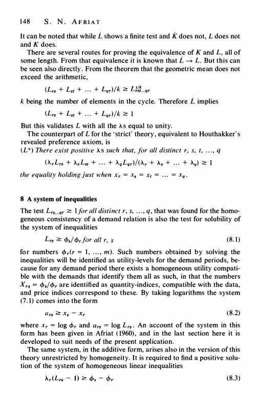
148 S . N . A F R I A T

It can be noted that while L shows a finite test and k does not, L does not and K does.

There are several routes for proving the equivalence of K and L, all of some length. From that equivalence it is known that L --"'? L. But this can be seen also directly . From the theorem that the geometric mean does not exceed the arithmetic,

(Lrs + Lst + . . . + Lqr)/k 2= M�Lqr

k being the number of elements in the cycle. Therefore L implies

(Lrs + Lst + . . . + Lqr)/k 2= 1

But this validates L with all the >.. s equal to unity. The counterpart of L for the ' strict' theory, equivalent to Houthakker' s

revealed preference axiom, is (L*) There exist positive >.. s such that, for all distinct r, s, t, . . . , q

(ArLrs + As Lst + . . . + AqLqr)/(Ar + >... + . . . + Aq) 2= 1

the equality holding just when Xr = X8 = x1 = . . . = Xq .

8 A system of inequalities

The test Lrs . . . qr 2= lfor all distinct r, s, . . . , q , that was found for the homo­geneous consistency of a demand relation is also the test for solubility of the system of inequalities

Lrs 2= </>./ </>r for all r, s (8. 1 )

for numbers </>r(r = l , . . . , m). Such numbers obtained by solving the inequalities will be identified as utility-levels for the demand periods, be­cause for any demand period there exists a homogeneous utility compati­ble with the demands that identify them all as such, in that the numbers Xr8 = </>8/</>r are identified as quantity-indices, compatible with the data, and price indices correspond to these. By taking logarithms the system (7. 1) comes into the form

(8.2)

where Xr = log </>r and Ors = log Lrs . An account of the system in this form has been given in Afriat ( 1960) , and in the last section here it is developed to suit needs of the present application.

The same system, in the additive form, arises also in the version of this theory unrestricted by homogeneity. It is required to find a positive solu­tion of the system of homogeneous linear inequalities

(8.3)

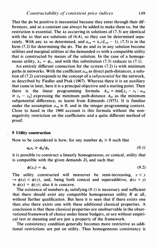
Constructability of consistent price indices 1 49

That the cps be positive is inessential because they enter through their dif­ferences, and so a constant can always be added to make them so, but the restriction is essential . The As occurring in solutions of (7. 3) are identical with the As that are solutions of (6.4), so they can be determined sepa­rately . With any AS so determined, and Grs = Ar(Lrs - 1) , (7.3) is in the form (7 .2) for determining the cps. The cps and As in any solution become utilities and marginal utilities at the demanded xs with a compatible utility that is constructed by means of the solution. In the case of a homoge­neous utility, Ar = <Pr , and with this substitution (7.3) reduces to (7. 1 ) .

An entirely different connection for the system (7.2) i s with minimum paths in networks . With the coefficient Grs as direct path-distances, a solu­tion of (7.2) corresponds to the concept of a subpotential for the network, as described by Fiedler and Ptak ( 1%7) . Whereas there it is an auxiliary that came in later, here it is a principal objective and a starting point. Then there is the linear programming formula Ali = min[x; - x1 : Grs ;::::: Xr - x8] expressing the minimum path-distance AiJ as the minimum subpotential difference, as learnt from Edmunds ( 1973) . It is familiar under the assumption ars ;::::: 0, and in the integer programming context. Close to hand in the 1960 account is this formula without the non­negativity restriction on the coefficients and a quite different method of proof.

9 Utility construction

Now to be considered is how, for any number <Pt > 0 such that

llsXt 2:: <Ptf <Ps (9. 1 )

it is possible to construct a linearly homogeneous, or conical , utility that is compatible with the given demands Dt and such that

(9.2)

The utility constructed will moreover be semi-increasing, x < y - cp(x) < cp(y) , and, being both conical and superadditive, cp(x + y) ;::::: cp(x) + cp(y) ; also it is concave.

The existence of numbers <Pt satisfying (9 . 1 ) is necessary and sufficient that there should exist any compatible homogeneous utility R at all , without further qualification. But here it is seen that if there exists one then also there exists one with these additional classical properties . A conclusion is that these classical properties are unobservable in the obser­vational framework of choice under linear budgets, or are without empiri­cal test or meaning and are just a property of the framework.

The consistency condition generally becomes more restrictive as addi­tional restrictions are put on utility . Thus homogeneous consistency is

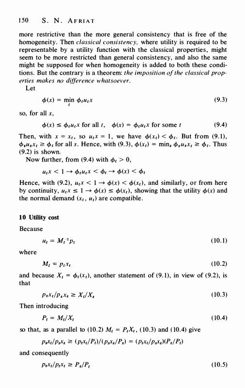
1 50 S . N . A F R I A T

more restrictive than the more general consistency that is free of the homogeneity. Then classical consistency, where utility is required to be representable by a utility function with the classical properties, might seem to be more restricted than general consistency, and also the same might be supposed for when homogeneity is added to both these condi­tions. But the contrary is a theorem: the imposition of the classical prop­erties makes no difference whatsoever.

Let

<f>(x) = min <f>tutx t

so, for all x,

(9.3)

<f>(x) ::; <f>tUtX for all t, <f>(x) = <f>tUtX for some t (9.4)

Then, with x = xi . so UtX = 1 , we have <f>(xt) < <f>t . But from (9. 1 ) , </>3u8x1 2:: <f>t for all s . Hence, with (9. 3) , <f> (xt) = min. <f>sUsXt 2:: <f>, . Thus (9.2) is shown.

Now further, from (9.4) with <f>t > 0,

UtX < 1 � <f>tUtX < <f>t � <f>(x) < <f>t

Hence, with (9.2) , UtX < 1 � <f>(x) < <f>(xt) , and similarly, or from here by continuity, UtX ::; 1 � <f>(x) ::; <f>(xt) , showing that the utility <f>(x) and the normal demand (xi . u1) are compatible .

1 0 Utility cost

Because

where

( 10. 1 )

( 10 .2)

and because X1 = <f>t (Xt), another statement of (9. 1 ) , in view of (9.2), is that

PsXtf PsXs 2:: Xi/ X8

Then introducing

Pt = MtfXt

so that, as a parallel to (10 .2) Mt = PtXi . ( 10.3) and ( 10.4) give

P.Xtf P.Xs 2:: (PtXtf Pt)/ (P.Xs/ Ps) = (ptxtf P.Xs)(P./ Pt)

and consequently

PsXi/ PtXt 2:: Ps/ Pt

( 10. 3)

( 10.4)

( 10.5)

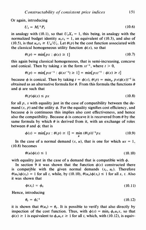
Constructability of consistent price indices

Or again, introducing

U1 = M(1P1

1 5 1

( 10.6)

in analogy with ( 10. 1 ) , so that U1X1 = 1 , this being, in analogy with the normalized budget identity u1x1 = 1 , an equivalent of ( 10.3) , and also of ( 10.5), is that u8x1 2': Us/ U1 • Let O(p) be the cost function associated with the classical homogeneous utility function cf>(x), so that

O(p) = min[px : cf>(x) 2': l ] ( 10.7)

this again being classical homogeneous, that is semi-increasing, concave and conical . Then by taking x in the form xr1 , where t > 0,

O(p) = min[pxt-1 : cf>(xt-1) 2': 1 ] = min[pxt-1 : cf>(x) 2': t]

because cf> is conical . Then by taking t = cf>(x), O(p) = min.x px(cf>(x))-1 is obtained as an alternative formula for (}. From this formula the functions (} and cf> are such that

O(p)cf>(x) :s; px ( 10.8)

for all p, x with equality just in the case of compatibility between the de­mand (x, p) and the utility cf>. For the equality signifies cost efficiency, and because cf> is continuous this implies also cost effectiveness, and hence also the compatibility. Because cf> is concave it is recovered from (} by the same formula by which (} is derived from it, with an exchange of roles between (} and cf>; that is

cf>(x) = min[px : O(p) 2': 1] = min (O(p))-1px ( 10.9) p

In the case of a normal demand (x, u), that is one for which ux = 1 , ( 10.8) becomes

(}(u)cf>(x) :s; 1 ( 10. 10)

with equality just in the case of a demand that is compatible with <f>. In section 9 it was shown that the function <f>(x) constructed there

is compatjble with the given normal demands (x1 , u1 ) . Therefore O(ui)<f>(x,) = 1 for all t, while, by ( 10. 10), O(u8)<f>(x1) :s; 1 for all s, t. Also it was shown that

Hence, introducing

01 = </>11

( 10. 1 1)

( 10. 12)

it is shown that O(u1) = 01 • It is possible to verify that also directly by inspection of the cost function. Thus, with <f>(x) = min1 <f>1 u1x, so that <f>(x) 2': 1 is equivalent to <f>1u1x 2': 1 for all t, which, with ( 10. 12), is equiv-

1 52 s . N . A F R I A T

alent to UtX ;:=: (Jt for all t , the cost function in ( 10 .7) is also

(J(u) = min[ux : UtX ;:=: 9t] ( 10. 1 3)

so that (J(ut) ;:=: (Jt . Therefore, by ( 10. 1 1 ) and ( 10. 12), (J(ut)cf>(xt) ;:=: 1 . Then UtXt = 1 with ( 10 . 10) shows that (J(ut)cf>(xt) = 1 and hence, again with ( 10. 1 1) and ( 10. 12), that (J(ut) = (Jt .

By the linear programming duality theorem (Dantzig 1963) applied to ( 10. 13) , another formula for the cost function is

(J(u) = max [ L stet : L StUt :S u J ( 10. 14)

Then, as known from the theory of linear programming, for any x, (J(u) :S ux for all u if and only if x solves ( 10. 13) . Similarly, with the (Jt now variable while u is fixed, for any St , (J(u) ;:=: 'L St (Jt for all (Jt if and only if the St solve ( 10. 14).

If the (Jt are a strict solution of (9. 1 ) , that is U8Xt > cf>t! cf>s (s I t) , then x = Xt9t is the unique solution of ( 10. 1 3) when u = Ut . In just that case (J(u) is differentiable at the point u = Ut · In that case (J is locally linear, and has a unique support gradient, and the differential gradient which now exists coincides with it. Thus in this case (J(u) :S ux for all u, and (J(ut) = UtX if and only if x = Xt 9i . so (J(u) has gradient Xt 9t at u = Ut ·

It can be added that this entire argument could have gone just as well with an interchange of roles between u and x. By solving U8Xt ;:=: (}3/(Jt for the (Jt , a cost function (J could be constructed first, with the form originally given to cf>, and then cf> could have been derived. Also, cf> need not have been given the polyhedral form (9.5). It could have been given the poly­tope form ( 10. 13) or ( 10 . 14) . Then (J would have had the polyhedral form (9. 5).

1 1 Price and quantity

The method established for the determination of index numbers can be stated in a way that treats price and quantity both simultaneously and in a symmetrical fashion. With the given demands (Xt , Pt), numbers (Xt , Pt) should satisfy

PsXt ;:=: PsXt for all s, t

Then, in particular,

PtXt = PtXt

Then division of ( 1 1 . 1) by ( 1 1 .2) gives

PsXt/ PtXt ;:=: Ps/ Pt

( 1 1 . 1)

( 1 1 .2)

( 1 1 .3)

Constructability of consistent price indices

as a condition for the 'price levels ' , and also

PsXi/ PsXs 2: Xi/ Xs

1 5 3

( 1 1 .4)

for 'quantity levels' . Reversely, starting with a solution Pt of ( 1 1 .3), let Xt be determined from ( 1 1 . 2) . Then Xt is a solution of ( 1 1 . 4) and the Pt and Xt together make a solution of ( 1 1 . 1 ) . Just as well, the procedure could start with a solution Xt of ( 1 1 .4) and go on similarly .

It has been established that the existence of solutions to these inequal­ities is necessary and sufficient for homogeneous consistency of the de­mand data. The investigation now concerns the identification of the numbers P rs = P8/ Pr obtained from solutions with all possible price indi­ces that are compatible with the data, that is, derivable on the basis of compatible homogeneous utilities . Then it will be possible to go further with a description of all possible price indices in terms of closed intervals specified by formulae for their end-points , or limits .

For any utility order R, the derived utility - cost function p (p, x) = min[py : yRx] is defined for all p, x if the sets Rx are closed. If R is a com­plete order and the sets Rx, xR are closed then, for any p, p(p, x) is a util­ity function representing R (see Afriat, 1979). It follows that, for any p and q, there exists an increasing function w(t), independent of x and carrying p, q as parameters, such that p (p, x) = w(p(q, x)) for all x.

If R is conical then so is p(p, x) as a function of x, for any p. In that case so is w(t) as a function of t. But a conical function of one variable must be homogeneous linear, so w(t) has the form wt where w is a function of p, q independent of x. That is, p(p, x)/p(q, x) = w is independent of x. Then w must have the form w = 8(p)/8(q) where O(p) is a function of p alone, so it follows that p(p, x)/(8(p) must be a function of x alone, and so p(p, x) = 8(p)cf>(x), where 8, cf> are functions p, x alone. Now cf> must be a utility that represents R, and be conical because p is conical in x. Then the condition for cf> to be quasi-concave is that the sets Rx be convex. But be­cause cf> is conical this is also the condition that cf> be concave (Berge, 1963). Moreover, because in any case p(p, x) is concave conical in p, so also is O(p) .

The reflexivity of R gives in any case p(p, x) :s; px, so now O(p)cf>(x) :s; px for all x. Hence, for all p, 8(p) :s; minx px(cf>(x))-1, while p(p, x) = px for some x gives O(p)cf>(x) = px for some x, so that now 8(p) = min px(cf>(xW1• Similarly cf>(x) :s; minp(O(p))-1 px. Then let (/>(x) = minp (8(p))-1px, so cf>(x) :s; (/>(x) for all x and (/> is concave conical . Then, for any x, cf>(x) = (/>(x) is equivalent to O(p)cf>(x) = px for some p. The condition for this to be so for any x is that cf>(x) be quasi-concave, having a quasi-support p at x, for which

PY < px - cf>(y) < cf>(x) , PY :s; px - cf>(y) :s; cf>(x)

1 54 s . N . A F R I A T

in other words the demand (x, p) is compatible with x for some p. This condition, which means that, with choice governed by cf>, x could be de­manded at some prices, can define compatibility between cf> and x. The condition that cf> be compatible with all x is just that it be quasi-concave, and that now is equivalent to <f>(x) = (/)(x) for all x. In any case, any x com­patible with cf> is also compatible with (/) . Hence, if utility R is constrained by compatibility with given demands, if cf> is acceptable then so is (/) , and moreover cf> and (/) have the same conjugate price function 8. This suggests that , instead of constructing a utility cf> compatible with the data having a concave form that is a generally unwarranted restriction on util­ity and, for all we know now, might make some added restriction on price-index values, it is both possible and advantageous to construct the price function 8 first instead, and so be free of such a suspicion. It has already been remarked that this might have been done instead, following an identical procedure as that for the cf>, so in fact that issue is already dis­posed of. From any compatible homogeneous utility a price function 8 is derived, giving the Pr = 8(pr) as a system of 'price-levels' compatible with the data, and determining the Prs = Psi Pr as compatible prices . But the possible such Pr are already identified with the possible solutions of ( 1 1 .3) . Also, for any solution Pr and the (J that must exist, the Xr deter­mined from ( 1 1 .2) have the identification Xr = <f>(xr) where cf>(x) = minp (8(p))-1px. This cf> is concave conical . But also any other <P* , not necessary concave but having the same conjugate 8, would do, so there is no inherent restriction to concave utilities here . For such a cf>* , generally <f>* (x) ::S cf>(x) , while <f>*(xr) = <f>(xr) for all r , and all that is re­quired of cf>* is that fJ(x) = minp px(<f>* (x))-1, and there are many cf>* for which this is so, that given being just one.

The argument in this section permits by-passing complications of the argument involving 'critical cost functions' that was used formerly , such as in the exposition of Afriat ( 1977b) for the special case of just two demand-periods. An interesting point is that the care taken in both argu­ments to avoid imposing on a compatible utility the requirement that also it be concave makes no difference at all to the range of possible values for a price-index .

12 Extension and exhaustion properties

For any coefficients ar8(r, s = 1 , . . . , k) , consider the system S(a) of simultaneous linear inequalities

ars 2:: Xs - Xr ( 12 . 1 )

to be solved for numbers Xr . This is an alternative form for the system (7 . 1 ) , and the form that applies directly to the system (7.3). Introduce

Constructability of consistent price indices

chain-coefficients

Grt; ... ks = ari + GiJ + · · · + aks

so that

ar . . . s ... t = ar . .. s + a •.. . t If the system S(a) has a solution x then

so by addition,

ar . . . s 2: Xs - Xr

In particular ar ... r 2: Xr - Xr = 0, so that ar ... r 2: 0, that is,

ari + a;; + . . . + akr 2: 0

1 55

( 12.2)

( 12.3)

( 12.4)

( 12 .5)

for every cyclic sequence of elements r, i, j, . . . , k, r. This can be called the cyclical non-negativity condition C on the system S(a), and it has been seen necessary for the existence of a solution. Because

ar ... s . . . s . . . r = ar . . . s . . . r + a •... s

the coefficient on a cycle with a repeated element s can be expressed as a sum of terms that are coefficients on cycles where the repetition multiplic­ity is reduced, and this decomposition can be performed on those terms and so forth until an expression is obtained with only simple cycles, without repeated elements. From this it follows that the condition C is equivalent to the same condition on cycles that are restricted to be simple, or have elements all distinct.

Under the condition C,

ar ... s . . . s . . . t = ar ... s ... t + a •...• 2: ar ... s . . . t so the cancellation of a loop in a chain does not increase the coefficient along it. It follows that the derived coefficient

Ars = min ar;; ... s ij . . . exists for any r, s and moreover

A - a rs - rij ... s

( 12.6)

( 12.7)

for some simple chain rij . . . s from r to s. Thus C is sufficient for the exis­tence of the derived coefficients . Also it is necessary. For if a •... s < 0 then for any r, t by taking the chain that goes from r to t, following the loop s . . . s any number K of times and then going from s to t, we have

Art � ars + Kas . . . s + a81 � - oo(K � oo) ( 12 .8)

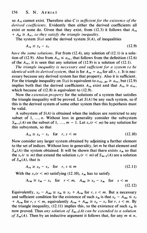
156 S. N . A F R I A T

so Art cannot exist. Therefore also C is sufficient for the existence of the derived coefficients . Evidently then either the derived coefficients all exist or none do. Given that they exist, from ( 12.3) it follows that Ars + Ast � Art , so they satisfy the triangle inequality .

The system S(a) and the derived system S(A), of inequalities

( 1 2.9)

have the same solutions . For from ( 12.4), any solution of ( 12 . 1 ) is a solu­tion of ( 1 2.9). Also from Ars ::S Ors , that follows from the definition ( 12.6) of the Ars , it is seen that any solution of ( 1 2.9) is a solution of ( 1 2. 1 ) .

The triangle inequality is necessary and sufficient for a system to be identical with its derived system, that is for Ars = Ors for all r, s . It is nec­essary because any derived system has that property. Also it is sufficient . For the triangle inequality on S(a) is equivalent to arij . . . ks � Ors , but ( 12.9) implies both that the derived coefficients Ars exist and that Ars � Ors , which because of ( 12 .8) is equivalent to ( 12.9) .

Now the extension property for the solutions of a system that satisfies the triangle inequality will be proved. Let S(A) be any such system, so if this is the derived system of some other system then this hypothesis must be valid .

A subsystem of S(A) is obtained when the indices are restricted to any subset of 1 , . . . , n . Without loss in generality consider the subsystem Sm-1 (A) on the subset of 1 , . . . , m - 1 . Let Xr (r < m) be any solution for this subsystem, so that

Ars � Xs - Xr for r, s < m ( 1 2. 10)

Now consider any larger system obtained by adjoining a further element to the set of indices. Without loss in generality, let m be that element and Sm(A) the system obtained. It will be shown that there exists Xm so that the Xr (r ::S m) that extend the solution Xr(r < m) of Sm-l (A) are a solution of Sm(A), that is

Ars � Xs - Xr for r, s ::S m

With the Xr (r < m) satisfying ( 12 . 10), Xm has to satisfy

( 12 . 1 1)

Arm � Xm - Xr for r < m, Ams � Xs - Xm for s < m ( 12 . 12)

Equivalently, Xs - Ams ::S Xm ::S Xr + Arm for r, s < m. But a necessary and sufficient condition for the existence of such Xm is that x. - Ams ::S Xr + Arm for r, s < m, equivalently Arm + Ams � X8 - Xr for r, s < m . By the triangle inequality, ( 12. 1 1 ) implies this , so the existence of such Xm is now proved. Thus any solution of Sm_1(A) can be extended to a solution of Sm(A) . Then by an inductive argument it follows that, for any m ::S n ,

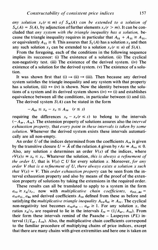
Constructability of consistent price indices 1 57

any solution Xr (r :S m) of Sm (A) can be extended to a solution of Sn (A) = S(A), by adjunction offurther elements Xr (r > m). It can be con­cluded that any system with the triangle inequality has a solution, be­cause the triangle inequality requires in particular that Au + Au :2: Au , or equivalently Au :2: 0. This assures that Si (A) has a solution Xi and then any such solution Xi can be extended to a solution Xr (r :S n) of S(A) .

From the foregoing, each of the conditions in the following sequence implies its successor: (i) The existence of a solution. (ii) The cyclical non-negativity test. (iii) The existence of the derived system. (iv) The existence of a solution for the derived system. (v) The existence of a solu­tion.

It was shown first that (i) - (ii) - (iii). Then because any derived system satisfies the triangle inequality and any system with that property has a solution, (iii) � (iv) is shown. Now the identity between the solu­tions of a system and its derived system shows (iv) � (i) and establishes equivalence between all the conditions , in particular between (i) and (ii).

The derived system S(A) can be stated in the form

- Asr :5 x. - Xr :5 Ars (r :5 s)

requiring the differences Xs - Xr (r s; s) to belong to the intervals (- Asr , Ar8) . The extension property of solutions assures also the interval exhaustion property, that every point in these intervals is taken by some solution. Whenever the derived system exists these intervals automati­cally are all non-empty.

An order U of the indices determined from the coefficients Ars is given by the transitive closure U = A of the relation A given by rAs = Ars s; 0. Also, any solution x determines an order V(x) of the indices , where rV(x)s = x8 s; Xr . Whatever the solution, this is always a refinement of the order U, that is V(x) C U for every solution x. Moreover, for any order V that is a refinement of U, there always exists a solution x such that V(x) = V. This order exhaustion property can be seen from the in­terval exhaustion property and also by means of the proof of the exten­sion property of solutions by taking the extensions in the required order.

These results can all be translated to apply to a system in the form ars :2: X8/Xr , now with multiplicative chain coefficients, ariJ . .. ks = ar;aii . . . aks and derived coefficients Ars defined from these as before and satisfying the multiplicative triangle inequality ArsAst :2: Art . The cyclical non-negativity test becomes ar.ast . . . aqr :2: l . For any solution x, the ratios X8/Xr are required to lie in the intervals lrs = ( 1 /A8r , Ar8) . From their form these intervals remind of the Paasche - Laspeyres (PL) in­terval ( 1 / L8r , Lr8) . Also, the multiplicative chain coefficients correspond to the familiar procedure of multiplying chains of price indices , except that there are many chains with given extremities and here one is taken on

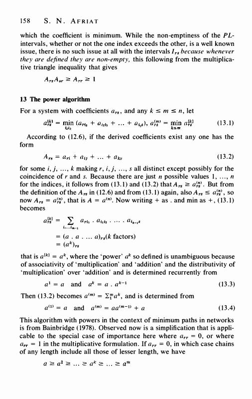
1 5 8 s . N . A F R I A T

which the coefficient is minimum. While the non-emptiness of the PL­intervals, whether or not the one index exceeds the other, is a well known issue, there is no such issue at all with the intervals lrs because whenever they are defined they are non-empty, this following from the multiplica­tive triangle inequality that gives

13 The power algorithm

For a system with coefficients ars , and any k s; m :s: n , let

( 1 3 . 1 )

According to ( 12.6), if the derived coefficients exist any one has the form

( 13 .2)

for some i, j, . . . , k making r, i, j, . . . , s all distinct except possibly for the coincidence of r and s. Because there are just n possible values 1 , . . . , n for the indices , it follows from ( 13 . 1 ) and ( 13 .2) that Ars � aW . But from the definition of the Ars in ( 12.6) and from ( 13 . 1 ) again, also Ars ::5 aW , so now Ars = a��> , that is A = a<n>. Now writing + as . and min as + , ( 13 . 1 ) becomes

a��l = L ari1 • a1i12 • • • • • a1._,s i, . . . i,,.-1

= (a . a . . . . a)r8(k factors) = (ak)rs

that is a CkJ = ak, where the 'power' ak so defined is unambiguous because of associativity of 'multiplication' and 'addition' and the distributivity of 'multiplication' over 'addition' and is determined recurrently from

a1 = a and ak = a . ak-i

Then ( 1 3 .2) becomes a<m> = 2::_"ak, and is determined from

aw = a and a<m> = aa<m-t> + a

( 13 .3)

( 1 3 .4)

This algorithm with powers in the context of minimum paths in networks is from Bainbridge ( 1978) . Observed now is a simplification that is appli­cable to the special case of importance here where arr = 0, or where arr = 1 in the multiplicative formulation. If arr = 0, in which case chains of any length include all those of lesser length, we have

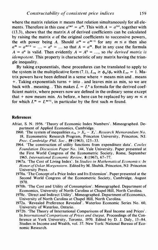
Constructability of consistent price indices 1 5 9

where the matrix relation :=::: means that relation simultaneously for all ele­ments. Therefore in this case a<m> = am. This with A = a<n>, together with ( 13 .3) , shows that the matrix A of derived coefficients can be calculated by raising the matrix a of the original coefficients to successive powers, the nth power being A. Should am = am-i for any m s; n then also am = am+i = . . . = an = . . . so that A = am. But in any case the formula A = an is valid . Then evidently A = A2 = . . . , so the derived matrix is idempotent. This property is characteristic of any matrix having the trian­gle inequality .

By taking exponentials, these procedures can be translated to apply to the system in the multiplicative form (7. 1 ) , Lrs :=::: <f>sl<f>r with Lrr = 1 . Ma­trix powers have been defined in a sense where + means min and . means + . Taking exponentials turns + into . and leaves min as min, so we are back with . meaning . . This makes i = L n a formula for the derived coef­ficient matrix, where powers now are defined in the ordinary sense except that + now means min. As before, n here can be replaced by any m s; n for which L m = L m+i , in particular by the first such m found.

References

Afriat, S. N. 1956. 'Theory of Economic Index Numbers' . Mimeographed. De­partment of Applied Economics, Cambridge.

1960. 'The system of inequalities ars > x. - Xr' . Research Memorandum No. 18, Econometric Research Program, Princeton University, Princeton, NJ. Proc. Cambridge Phil. Soc . , 59 ( 1963) , 125-33.

1964. The construction of utility functions from expenditure data' . Cowles Foundation Discussion Paper No. 144, Yale University . Paper presented at the First World Congress of the Econometric Society , Rome, September 1965 . International Economic Review, 8 ( 1967), 67-77.

1967a. 'The Cost of Living Index' . In Studies in Mathematical Economics: In Honor ofOskar Morgenstern . Edited by M. Shubik. Princeton, NJ: Princeton University Press.

1970a. 'The Concept of a Price Index and Its Extension' . Paper presented at the Second World Congress of the Econometric Society , Cambridge, August 1970.

1970b. 'The Cost and Utility of Consumption' . Mimeographed. Department of Economics, University of North Carolina at Chapel Hill, North Carolina.

1970c . 'Direct and Indirect Utility' . Mimeographed. Department of Economics, University of North Carolina at Chapel Hill, North Carolina.

1972a. 'Revealed Preference Revealed' . Waterloo Economic Series No. 60, University of Waterloo, Ontario.

1972b. 'The Theory of International Comparisons of Real Income and Prices' . In International Comparisons of Prices and Output, Proceedings of the Con­ference at York University , Toronto , 1970. Edited by D. J. Daly , 13 -84. Studies in Income and Wealth, vol. 37. New York: National Bureau of Eco­nomic Research.

1 60 s . N . A F R I A T

1973. 'On a System of Inequalities in Demand Analysis: an Extension of the Classical Method' . International Economic Review, 14, 460-72.

1974. 'Sum-symmetric matrices ' . Linear Algebra and its Applications, 8, 129-40.

1976. Combinatorial Theory of Demand. London: Input - Output Publishing Co.

1977a. 'Minimum paths and subpotentials in a valuated network' . Research Paper 7704, Department of Economics, University of Ottawa.

1977b. The Price Index. Cambridge and New York: Cambridge University Press.

1978a. 'Index Numbers in Theory and Practice by R. G. D. Allen' . Canadian Journal of Economics, 11, 367-9.

1978b. 'Theory of the Price Index by Wolfgang Eichhorn and Joachim Voeller' . Journal of Economic Literature, 16, 129-30.

1979. Demand Functions and the Slutsky Matrix. Princeton, NJ: Princeton University Press.

1980. 'Matrix Powers: Classical and Variations' . Paper presented at the Matrix Theory Conference, Auburn University, Auburn, Alabama, 19-22 March 1980.

Allen, R. G. D. 1975. Index Numbers in Theory and Practice. London: Mac­millan.

Bainbridge, S. 1978. 'Power algorithm for minimum paths' , private com­munication . Department of Mathematics, University of Ottawa, Ontario.

Berge , C. 1963. Topological Spaces. New York: Macmillan . Berge , C. and Ghouila-Houri, A. 1965. Programming, Games and Transportation

Networks. London: Methuen & Co. New York: John Wiley and Sons. Dantzig, G. 1963. 'Linear Programming and Its Extensions ' . Princeton, NJ:

Princeton University Press. Edmunds, J . 1973 . ' Linear programming formula for minimum paths' , private

communication. Department of Combinatorics and Optimization, Faculty of Mathematics, University of Waterloo, Ontario .

Eichhorn, W. and Voeller, J. 1976. Theory of the Price Index: Fisher's Test Ap­proach and Generalizations. Berlin, Heidelburg and New York: Springer­Verlag.

Fiedler, M. and Ptak, V. 1967. ' Diagonally dominant matrices ' . Czech. Math J. , 17, 420-33.

Fisher, I . 1927. The Making of Index Numbers . Third edition. Boston and New York: Houghton Mifflin Company.

Geary , R. C. 1958. 'A note on the comparison of exchange rates and purchasing power between countries' . J. Roy Stat. Soc. A, 121, 97-9.

Hicks, J. R. 1956. A Revision of Demand Theory. Oxford: Clarendon Press. Houthakker, H. S. 1950. 'Revealed Preference and the Utility Function' , Econo­

mica, New Series, 17, 159-74. Samuelson, P. A. 1947. The Foundations of Economic Analysis. Cambridge ,

Mass . : Harvard University Press. Samuelson , P. A. and Swamy, S. 1974. ' Invariant Economic Index Numbers and

Canonical Duality: Survey and Synthesis ' . American Economic Review, 64, 566-93 .

Shephard, R. W. 1953. Cost and Production Functions. Princeton, NJ: Princeton University Press.

Constructability of consistent price indices 1 6 1

Theil, H . 1960. 'Best linear index numbers of prices and quantities' . Econome­trica, 28, 464-80.

1975 - 1976. Theory and Measurement of Consumer Demand. Two volumes. Amsterdam: North-Holland Publishing Company.

1979. The System-wide Approach to Microeconomics. The University of Chi­cago Press.

Yen, J. Y. 1975. Shortest Path Network Problems. Meisenheim am Gian : Verlag Anton Hain.

7 The economic theory of index numbers : a survey1

W. E . D I EWE R T

1 Introduction

The literature on index numbers is so vast that we can cover only a small fraction of it in this chapter. Frisch (1936) distinguishes three approaches to index number theory: (i) ' statistical' approaches, (ii) the test approach, and (iii) the functional approach, which Wold ( 1 953, p . 1 35) calls the pref­erence field approach and Samuelson and Swamy ( 1974, p. 573) call the economic theory of index numbers. We shall mainly cover the essentials of the third approach. In the following two sections, we define the dif­ferent index number concepts that have been suggested in the literature and develop various numerical bounds. Then in section 4, we briefly survey some of the other approaches to index number theory. In section 5, we relate various functional forms for utility or production functions to various index number formulae. In section 6, we develop the link between 'flexible' functional forms and 'superlative' index number formulae. The final section offers a few historical notes and some comments on some re­lated topics such as the measurement of consumer surplus and the Divisia index.

2 Price indexes and the Koniis cost of living index

We assume that a consumer is maximizing a utility function F(x) subject to the expenditure constraint prx = Lf=1 PiXi ::;; y where x = (xi. . . . , xN)T � ON is a non-negative vector of commodity rentals, p = (p1, . . . , PNf >> ON is a positive vector of commodity prices2 and y > 0 is expend­iture on the N commodities . We could also assume that a producer is maximizing a production function F(x) subject to the expenditure con­straint prx ::;; y where x � ON is now an input vector, p >> ON is an input price vector and y > 0 is expenditure on the inputs . In order to cover both the consumer and producer theory applications, we shall call the utility or production function F an aggregator function in what follows.

The consumer's (or producer's) aggregator maximization problem can be decomposed into two stages: in the first stage, the consumer (or pro-

1 63

1 64 W . E . D I E W E RT

ducer) attempts to minimize the cost of achieving a given utility (or out­put) level, and, in the second stage, he chooses the maximal utility (or output) level that is just consistent with his budget constraint.

The solution to the first stage problem defines the consumer's (or pro­ducer' s cost function C:

( 1 )

The cost function C turns out to play a pivotal role in the economic ap­proach to index number theory.

Throughout much of this chapter, we shall assume that the aggregator function F satisfies the following Conditions /: F is a real valued function of N variables defined over the non-negative orthant 0 = {x: x ;:::: ON} which has the following three properties : (i) continuity, (ii) increasingness3 and (iii) quasi-concavity. 4

Let U be the range of F. From l(i) and (ii), it can be seen that U = {u: ii :S u :S U} where ii = F(ON) < u. Note that the least upper bound u could be a finite number or + oo. In the context of production theory, typically ii = 0 and u = + oo, but, for consumer theory applications, there is no reason to restrict the range of the utility function F in this manner.

Define the set of positive prices p = {p: p >> ON}. It can be shown that (see Diewert, 1978c) if F satisfies Conditions I , then the cost function C defined by ( 1 ) satisfies the following Conditions II:

(i) C(u, p) is a real valued function of N + 1 variables defined over U x P and is jointly continuous in (u, p) over this domain.

(ii) C(ii, p) = 0 for every p E P. (iii) C(u, p) is increasing in u for every p E P; i .e . , if p E P, u' , u" E U,

with u' < u", then C(u ' , p) < C(u", p). (iv) C(u, p) = + oo for every p E P; i .e . , if p E P, un E U, limn un = ii,

then limn C(un, p) = + oo. (v) C(u, p) is (positively) linearly homogenous in p for every u E U:

i.e. u E U, A. > 0, p E P implies C(u , A.p) = A.C(u, p). (vi) C(u, p) is concave in p for every u E U; i.e . , if p' >> ON, p" >> ON,

0 s; A. s; 1 , u E U, then C(u, A.p' + ( 1 - A.) p") ;:::: A.C(u, p') + ( 1 - A.)C(u, p").

(vii) C(u, p) is increasing in p for u > ii and u E U. (viii) C is such that the function F*(x) = maxu{u : prx ;:::: C(u, p) for every

p E P, u E U} is continuous for x ;:::: ON. For some of the theorems to be presented in this chapter, we can

weaken the regularity conditions on the aggregator function F to just con­tinuity from above. 5 Under this weakened hypothesis on F, the cost func­tion C defined by ( 1 ) will still satisfy many of the properties in Conditions II above.6

Finally , some of the theorems below make use of the following

The economic theory of index numbers 1 65

(stronger) regularity conditions on the aggregator function: we say that F is a neoclassical aggregator function if it is defined over the positive orthant {x: x >> ON} and is (i) positive, i .e . F(x) > 0 for x >> ON, (ii) (pos­itively) linearly homogeneous, and (iii) concave over {x: x >> ON} . Under these conditions (let us call them Conditions Ill) F can be extended to the non-negative orthant !l, and the extended F will be non-negative, linearly homogeneous, concave, increasing and continuous over !l (see Diewert, 1978c). Moreover, if F is neoclassical, then F's cost function C factors into

C(u, p) = u C( l , p) = u c(p) (2)

for u � 0 and p >> ON where c(p) = C(l , p) is F's unit cost function. It can be shown that c satisfies the same regularity conditions as F; i .e . c is also a neoclassical function. Also, if we are given a neoclassical unit cost function c, then the underlying aggregator function F can be defined for x >> ON by

F(x) = maxu{u : C(u, p) ::5 prx for every p > ON} = maxu{u : u c(p) ::5 prx for every p � ON, prx = 1} = minp{ l/c(p): p � ON, prx = l } (3)

= 1/maxp{c(p) : prx = 1 , p � ON} (4)

Now that we have disposed of the mathematical preliminaries, we can define the Koniis ( 1924) cost of living index7 Px: for p0 >> ON, p1 >>ON and x > ON

(5)

Thus Px depends on three sets of variables : (i) p0, a vector of period 0 or base period prices, (ii) p1 , a vector of period 1 or current period prices,8 and (iii) x, a reference vector of quantities .9 In the consumer context, Px can be interpreted as follows. Pick a reference indifference surface in­dexed by the quantity vector x > ON. Then Px(p0, p1 , x) is the minimum cost of achieving the standard of living indexed by x when the consumer faces period 1 prices p1 relative to the minimum cost of achieving the same standard of living when the consumer faces period 0 prices p0• Thus Px can be interpreted as a level of prices in period 1 relative to a level of prices in period 0. If the number of goods is only one (i.e. N = 1 ), then it is easy to see that Px(p�, pl, X1) = PUP� for all X1 > 0.

Note that the mathematical properties of Px with respect to p0, p1 and x are determined by the mathematical properties of F and C given by Condi­tions I and II above. In particular, for A. > 0, p0 >> ON p1 >> ON and x >> ON, we have Px(p0, A.p0, x) = A and Px(p0, p1 , x) = 1/Px(p1 , p0, x) . Thus if period 1 prices are proportional to period 0 prices, then Px is equal

1 66 W . E . D I E W E RT

to the common factor of proportionality for any reference quantity vector x. However, if prices are not proportional , then in general Px depends on the reference vector x, except when preferences are homothetic as is shown in the following result.

Theorem 1 10 ((Malmquist ( 1953, p. 215) , Pollak ( 197 1 , p. 3 1) , Samuelson and Swamy ( 1974, pp. 569-70)): Let the aggregator function F satisfy Conditions I . Then P x(p0, p1, x) is independent of x if and only if F is ho­mo the tic .

Proof" If F is homothetic, then, by definition, there exists a continuous, monotonically increasing function of one variable G, with G(u) = 0 such that G[F(x)] = f(x) is a neoclassical aggregator function (i.e. f satisfies Conditions III above). Under these conditions, F's cost function decom­poses as follows: for u > 0, p >> ON,

C(u, p) = minx{pTx: F(x) ::::: u} = minx{pTx: G[F(x)] ::::: G(u)} = G(u)c(p) (6)

where c is the unit cost function which corresponds to the neoclassical ag­gregator function f Thus for p0 >> ON, p1 >> ON and x > ON, we have

Px(p0, pi , x) = C[F(x), p1]/ C[F(x) , p0] = G[F(x)]c(p1)/G[F(x)]c(p0) = c(p•)/c(po)

which is independent of x.

(7)

Conversely, if Px is independent of x, then we must have the factoriza­tion (7); i .e. we must have for every x >> ON, p >> ON

C(F(x) , p) = G[F(x)]c(p) (8)

for some functions G and c, whose regularity properties must be such that C satisfies Conditions II . It can be verified that the regularity conditions on C and the decomposition (8) imply that the functions c and G[F] both satisfy Conditions III, 11 so that, in particular, G[F(x)] is (positively) lin­early homogeneous in x. Thus F is homothetic . Q.E.D.

Thus in the case of a homothetic aggregator function, the Koniis cost of living index Px(p0, p1 , x) is independent of the reference quantity vector x and is equal to a ratio of unit cost functions, c(p1)/c(p0) .

If we knew the consumer's preferences (or the producer's production function), then we could construct the cost function C(u, p) and the Koniis price index Px. However, usually we do not know F or C and thus it is useful to develop non-parametric bounds on Px; i.e. bounds that do not depend on the functional form for the aggregator function F (or its cost function dual C).

The economic theory of index numbers 1 67

Theorem 2 (Lerner, 1935-36; Joseph, 1935-36, p. 149; Samuelson, 1947, p. 159; Pollak, 197 1 , p. 12): If the aggregator function F is continu­ous from above, then, for every p0 = (py, . . . ,p'J,f >> ON, p1 = (pL . . . , p°Nf >> ON and x > ON where F(.X) > F(ON),

· { 1/ o. · _ 1 N} < P' r o 1 -) mm, P1 Pt . 1 - , . . . , - K\P , p , x

:s; max1{Pl/ p?: i = 1 , . . . , N} (9)

i .e. PK lies between the smallest and the largest price ratio . Proof' Let p0 >> ON, p1 >> ON, x > ON where F(.X) > F(ON) and let xO �

ON and x1 � ON solve the following cost minimization problems:

C[F(.X) , p0] = minx{p0Tx: F(x) � F(.X)} = p0Tx0 > 0 ( 10)

C[F(.X), p1] = minx{P1Tx: F(x) � F(.X)} = p1Tx1 > 0 ( 1 1 )

. . C[F(.X), p1] = minx{P1Tx: F(x) � F(.X)} � minx{P1Tx: poTx � poTxO, x � ON}

since {x: F(x) � F(.X)} C {x: poTx � poTxo, x � ON}

= min1{pt(p0Tx0/pf): i = 1 , . . . , N} ( 1 2)

since the solution to the linear programming problem minx{P1T x: p0T x � p0T x0, x � ON} can be taken to be a corner solution. Similarly,

or

1/C[F(.X) , p0] :s; max1{pl/p? p1Tx1 : i = 1 , . . . , N} ( 1 3)

Since PK(p0, p1 , .X) = C[F(.X), p1]/ C[F(.X), p0] , ( 10) and ( 1 2) imply the lower limit in (9) while ( 1 1) and ( 13) imply the upper limit. Q.E.D.

The geometric idea behind the above algebraic proof is that the sets {x: p0Tx � p0TxO, x � ON} and {x: p1Tx1 � p1Tx1 , x � ON} form outer approxi­mations to the true utility (or production) possibility set {x: F(x) � F(.X)}. Moreover, it can be seen that the bounds on PK given by (9) are the best possible,12 i .e. if F(x) = p0Tx, then PK will attain the lower bound while, if F(x) = p1Tx, then PK will attain the upper bound in (9).

It is natural to assume that we can observe the consumer's (or produc­er's) quantity choices xO > ON and x1 > ON, made during periods 0 and 1 in addition to the prices which prevailed during those periods, p0 >> ON and p1 >> ON. In the remainder of this section, we shall also assume that the consumer (or producer) is engaging in cost minimizing behaviour during the two periods . Thus we assume:

poTxO = C[F(xO) , po] ; p1Tx1 = C[F(xl), pl] ; po, p1 >> ON; xo, x1 > ON ( 14)

1 68 W . E . D I E W E RT

Given the above assumptions , we now have two natural choices for the quantity vector x which occurs in the definition of the Koniis cost of living index Px(p0, p1 , x) : xO or x1 • The Laspeyres -Konus cost of living index is defined as Px(p0, p1 , x0) and the Paasche-Konus cost of living index is de­fined as P x(p0, p1 , x1) . 13 It turns out that the Laspeyres-Koniis index Px(p0, p1 , x0) is related to the Laspeyres price index PL(p0, p1 , x0, x1) = p1Tx0/p0TxO while the Paasche-Koniis index Px(p0, p1 , x1) is related to the Paasche price index Pp(p0, p1 , x0, x1) = p1Tx1/p0Tx1 .

Theorem 3 (Koniis, 1924, pp. 17- 19): Suppose F is continuous from above and ( 14) holds. Then

Px(Po, p' , xO) ::5 plTxo/porxo = PL and

Px(po, p1 , xl) � plTxI/pOTx1 = Pp,

Proof·

Px(po, p1 , xO) = C[F(xo) , pl]/C[F(xo), po] = C[F(x0), p1]/p0Tx0 using ( 14) = minx{P1Tx: F(x) � F(x0)}/p0TxO ::::; p1T xo I por xO

( 15)

( 16)

since x0 is feasible for the cost minimization problem (but is not necessar­ily optimal), which proves ( 15). Similarly,

Px(Po, p1 , xl) = p1T xl I C[F(xl) , po] = p1Tx1/min.r{p0Tx: F(x) � F(x1)} � plTxl/pOTxl

Corollary 3 . 1 (Pollak, 197 1 , p. 17):

Q.E.D.

min1{pifpf: i = 1, . . . , N} ::5 Px(Po, p1 , xo) ::5 p1Txo/porxo = PL ( 17)

Corollary 3.2 (Pollak, 197 1 , p. 18):

PP = P1rx1;porx1 ::5 Px(po, p1 , xl) ::5 max1{ptfpf: i = 1 , . . . , N} ( 1 8)

Corollary 3 .3 (Frisch, 1936, p. 25): If in addition, F is homothetic, then for x >> ON,

Pp = p1Tx1/porx1 ::5 Px(Po, p1 , x) ::5 plTxO/porxo = pL ( 19)

The first two corollaries follow from Theorems 2 and 3, while the third corollary follows from Theorems 1 and 2. Note that

N pL = P1rx0;porx0 = L (pljp�)(p�x'l/porxo)

i=l N = L (pl/p?)s? :s: max1{pl/p? : i = 1 , 2, . . . , N}

i=l

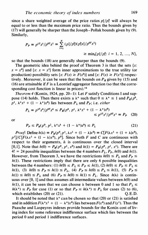
The economic theory of index numbers 1 69

since a share weighted average of the price ratios pl/ pf will always be equal to or less than the maximum price ratio. Thus the bounds given by ( 17) will generally be sharper than the Joseph-Pollak bounds given by (9). Similarly,

N Pp = p1rx1/porx1 = L (p}/p�)(p�x}/porx1)

i=l � min1{pl/pf : i = 1 , 2, . . . , N},

so that the bounds ( 18) are generally sharper than the bounds (9) . The geometric idea behind the proof of Theorem 3 is that the sets {x:

x = xO} and {x: x = x1} form inner approximations to the true utility (or production) possibility sets {x: F(x) � F(x0)} and {x: F(x) � F(x1)} respec­tively . Moreover, it can be seen that the bounds on PK given by ( 1 5) and ( 16) are attainable if F is a Leontief aggregator function (so that the corre­sponding cost function is linear in prices). 14

Theorem 4 (Koniis, 1924, pp. 20- 1) : Let F satisfy Conditions I and sup­pose ( 14) holds . Then there exists a A* such that 0 :s; A* :s; 1 and P�p0, p1 , A*x1 + ( 1 - A*)xO) lies between PL and Pp; i .e . either

PL = p1rx0;porxo ::5 PK(po, pi , A*x1 + ( 1 - A*)xo) ::5 P1rx1;porx1 = Pp (20)

or

(21 )

Proof· Define h(A) = P K(p0, p1, h1 + (1 - A)x0) = C[F(h1 + ( 1 + A)x0), p1]/C[F(h1 + (1 - A)x0), p0]. Since both F and C are continuous with respect to their arguments, h is continuous over the closed interval [0, 1 ] . Note that h(O) = PK(p0, p1 , xO) and h(l) = P�p0, p1 , x1) . There are 4! = 24 possible inequalities between the 4 numbers PL, Pp, h(O) and h(l) . However, from Theorem 3, we have the restrictions h(O) ::5 PL and Pp ::5 h(l) . These restrictions imply that there are only 6 possible inequalities between the 4 numbers : ( 1 ) h(O) ::5 PL ::5 Pp ::5 h(l) , (2) h(O) ::5 PP ::5 PL ::5 h(l), (3) h(O) ::5 Pp ::5 h( l) ::5 PL, (4) Pp ::5 h(O) ::5 PL ::5 h(l) , (5) Pp ::5 h(l) ::5 h(O) ::5 PL and (6) Pp ::5 h(O) :s; h( l) :s; PL. Since h(A) is contin­uous over [O, 1] and thus assumes all intermediate values between h(O) and h(l) , it can be seen that we can choose A between 0 and 1 so that PL :s; h(A *) ::5 PP for case ( 1 ) or so that Pp ::5 h(A *) ::5 PL for cases (2) to (6) , which establishes (20) or (21) . Q.E.D.

It should be noted that A* can be chosen so that (20) or (21) is satisfied and in addition F(A *x1 + ( 1 - A *)x0) lies between F(x0) and F(x1) . Thus the Paasche and Laspeyres indexes provide bounds for the Koniis cost of liv­ing index for some reference indifference surface which lies between the period 0 and period 1 indifference surfaces .

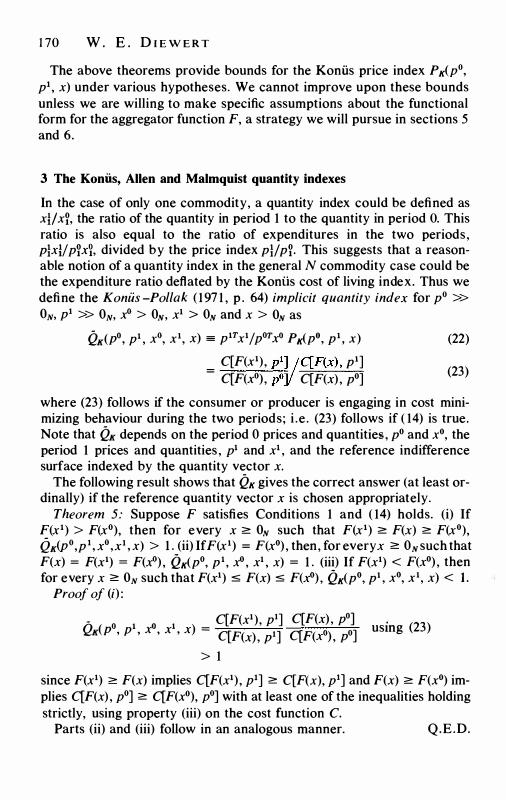
1 70 W . E . D I E W E R T

The above theorems provide bounds for the Koniis price index Px(p0, p1 , x) under various hypotheses. We cannot improve upon these bounds unless we are willing to make specific assumptions about the functional form for the aggregator function F, a strategy we will pursue in sections 5 and 6.

3 The Konus, Allen and Malmquist quantity indexes

In the case of only one commodity, a quantity index could be defined as xUxf, the ratio of the quantity in period 1 to the quantity in period 0. This ratio is also equal to the ratio of expenditures in the two periods, plx}/pfx7, divided by the price index plfpf. This suggests that a reason­able notion of a quantity index in the general N commodity case could be the expenditure ratio deflated by the Koniis cost of living index. Thus we define the Konus -Pollak ( 197 1 , p . 64) implicit quantity index for p0 >> ON, p1 >> ON, xO > ON, x1 > ON and x > ON as

Qx(Po, p1 , xO, x1, x) = p1rx1/porxo Px(po, p1 , x)

=

C[F(x1), p1J /C[F(x) , p1] C[F(x0), p0]/ C[F(x) , p0]

(22)

(23)

where (23) follows if the consumer or producer is engaging in cost mini­mizing behaviour during the two periods; i .e. (23) follows if ( 14) is true. Note that Qx depends on the period 0 prices and quantities, p0 and x0, the period 1 prices and quantities , p1 and x1 , and the reference indifference surface indexed by the quantity vector x.

The following result shows that Qx gives the correct answer (at least or­dinally) if the reference quantity vector x is chosen appropriately.

Theorem 5: Suppose F satisfies Conditions 1 and ( 14) holds. (i) If F(x1) > F(x0), then for every x 2: ON such that F(x1) 2: F(x) 2: F(x0), Qx(p0,p1 , x0,x1 , x) > l . (ii) IfF(x1) = F(x0) , then, for everyx 2: ON such that F(x) = F(x1) = F(xO) , Qx(p0, p1, x0 , x1 , x) = 1 . (iii) If F(x1) < F(x0) , then for every x 2: ON such that F(x1) s; F(x) s; F(x0) , Qx(p0, p1 , x0, x1, x) < l.

Proof of (i) :

- o 1 o 1 - C[F(x1), pl] C[F(x) , po] . (23) Qx(P ' p , x ' x , x) - C[F(x) , pl] C[F(xO) , po] usmg

> 1

since F(x1) 2: F(x) implies C[F(x1) , p1] 2: C[F(x), p1] and F(x) 2: F(x0) im­plies C[F(x) , p0] 2: C[F(x0), p0] with at least one of the inequalities holding strictly, using property (iii) on the cost function C.

Parts (ii) and (iii) follow in an analogous manner. Q.E.D.

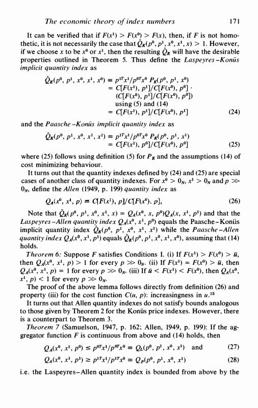
The economic theory of index numbers 1 7 1

It can be verified that if F(x1) > F(xO) > F(x), then, if F is not homo­thetic, it is not necessarily the case that QK(p0, p1 , x0, x1 , x) > 1 . However, if we choose x to be x0 or x1 , then the resulting QK will have the desirable properties outlined in Theorem 5. Thus define the Las peyre s -Konus implicit quantity index as

QK(po, p1 , xo, x1 , xo) = p1Tx1;p0Txo P�po, p1 , xO) = C[F(x1) , p1]/C[F(x0) , p0] ·

(C[F(x0), p1]/C[F(x0) , p0]) using (5) and ( 14)

= C[F(x1) , p1]/C[F(xO) , p1]

and the Paasche -Konus implicit quantity index as

QK(po, p1 , xo, x1 , xl) = p1Tx1/pOTxO PK(po, p1 , xl) = C[F(xl), po]/C[F(xo) , po]

(24)

(25)

where (25) follows using definition (5) for PK and the assumptions ( 14) of cost minimizing behaviour.

It turns out that the quantity indexes defined by (24) and (25) are special cases of another class of quantity indexes. For x0 > ON, x1 > ON and p >> ON, define the Allen ( 1949, p . 199) quantity index as

(26)

Note that Q�p0, p1 , x0, x1 , x) = QA(xO, x, p0)QA(x, x1 , p1) and that the Laspeyres -Allen quantity index QA(x0, x1 , p0) equals the Paasche-Koniis implicit quantity index QK(p0, p1 , x0, x1 , x1) while the Paasche -Allen quantity index QA(xO, x1 , p1) equals QK(p0, p1 , x0, x1 , x0) , assuming that ( 14) holds.

Theorem 6: Suppose F satisfies Conditions I. (i) If F(x1) > F(x0) > u, then QA(xO, x1 , p) > 1 for every p >> ON. (ii) If F(x1) = F(x0) > u, then QA(x0, x1 , p) = 1 for every p >> ON. (iii) If u < F(x1) < F(x0) , then QA(x0, x1 , p) < 1 for every p >> ON.

The proof of the above lemma follows directly from definition (26) and property (iii) for the cost function C(u, p) : increasingness in u. 15

It turns out that Allen quantity indexes do not satisfy bounds analogous to those given by Theorem 2 for the Koniis price indexes. However, there is a counterpart to Theorem 3 .

Theorem 7 (Samuelson, 1947, p. 162; Allen, 1949, p. 199): If the ag­gregator function F is continuous from above and ( 14) holds, then

QA (xo, x1 , po) :5 poT xl / poT xO = QL(Po' p1 , xo , x1) and (27)

QA(xo, x1 , pl) � p1Tx1/p1Tx0 = Qp(po, p1 , xo, xl) (28)

i .e . the Laspeyres-Allen quantity index is bounded from above by the

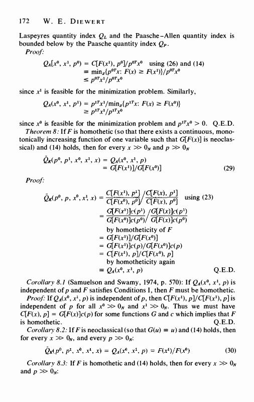
1 72 W . E . D I E W E RT

Laspeyres quantity index QL and the Paasche-Allen quantity index is bounded below by the Paasche quantity index Qp .

Proof" QA[x0, x1, p0) = C[F(x1) , p0]/p0Tx0 using (26) and ( 14)

= minx{p0Tx: F(x) � F(x1)}/p0Tx0 :5 poT x' I poT xO

since x' is feasible for the minimization problem. Similarly,

QA(x0, x1 , p1) = p1Tx1/min,,,{p1Tx: F(x) � F(x0)} � p'Tx'/p'TxO

since x0 is feasible for the minimization problem and p1Tx0 > 0. Q.E.D. Theorem 8: If F is homothetic (so that there exists a continuous, mono­

tonically increasing function of one variable such that G[F(x)] is neoclas­sical) and ( 14) holds, then for every x >> ON and p >> ON

Qx(p0, p1, x0, x' , x) = QA(x0, x1 , p) = G[F(x1)]/G[F(x0)]

Proof"

-0 0 1 _ C[F(x1), p'J /C[F(x) , p1]

Qx(P , p, x , x , x) - C[F(x0), PoV C[F(x), po] using (23)

= G[F(x1)]c(p1)/G[F(x)]c(p1) G[F(x0)]c(p0) G[F(x)]c(p0) by homotheticity of F

= G[F(x1)]/G[F(x0)] = G[F(x1)]c(p)/G[F(x0)]c(p) = C[F(x1) , p]/C[F(x0), p]

by homotheticity again = QA(x0, x1, p)

(29)

Q.E.D.

Corollary 8. 1 (Samuelson and Swamy, 1974, p . 570) : If QA(x0, x1, p) is independent of p and F satisfies Conditions I , then F must be homothetic.

Proof" If QA(xO, x1 , p) is independent of p, then C[F(x1), p]/C[F(x1), p] is independent of p for all x0 >> ON and x1 >> ON. Thus we must have C[F(x), p] = G[F(x)]c(p) for some functions G and c which implies that F is homothetic . Q.E.D.

Corollary 8.2: If F is neoclassical (so that G(u) = u) and ( 14) holds, then for every x >> ON, and every p >> ON:

(30)

Corollary 8.3: If F is homothetic and ( 14) holds, then for every x >> ON and p >> ON:

The economic theory of index numbers l 73

Qp = p1rx1/p1rxo ::5 Qx(po, pi , xo, xi , x) = QA(xO, xi , p) :s; Porxi/porxo = QL (3 1)

Proof' From (28),

Qp ::5 QA(xO, xi , pl) = Qx(Po, pi , xo, x1 , x) = QA(xo, xi , p) = QA(x0, x1 , p0) using (29) ::5 QL using (27)

Q.E .D.

Thus if the aggregator function is homothetic , then the Allen and Implicit Koniis quantity indexes coincide for all reference vectors p and x, and their common value is bounded from below by the Paasche quantity index Qp and above by the Laspeyres quantity index QL. Note that Qp and QL can be computed from observable data.

In the general case when F is not necessarily homothetic, the following results give bounds for Qx and QA .

Theorem 9: Let F satisfy Conditions I and suppose ( 14) holds. Then there exists a A.* such that 0 :s; A.* ::5 1 and Qx(xO, x1 , p0, p1 , A.* x1 + ( 1 - A. *)x0) lies between Qp and QL.

Proof: From Theorem 4, either (20) or (2 1) holds for Px(p0, p1 , A.*x1 + ( 1 - A. *)xO) for some A.* between 0 and 1 . If (20) holds, then, using defi­nition (22):

QL = (p1T xi/ por xO)/ Pp ::5 Qx(xo' x1 , po' pi ' A.* xi + ( 1 - A. *)xo) :s; (plTxl/pOTxO)/PL = Qp

Similarly , if (2 1) holds then Qp :s; Qx(xO, x1 , p0, p1 , A.* x1 + ( 1 - A. *)x0) ::5 QL. Q.E.D.

Theorem JO: Let F be continuous from above and suppose ( 14) holds. Then there exists a A.* such that 0 :s; A.* :s; 1 and QA (x0, x1 , A.* p1 + ( 1 - A. *)p0) lies between QL and Qp.

Proof' Define h(A.) = QA(x0, x1 , A.p1 + ( 1 - A.)p0) = C[F(x1), A.p1 + ( 1 - A.)p0]/C[F(x0), A.p1 + ( 1 - A.)p0]. Since F i s continuous from above , C(u, p) is continuous in p and thus h(A.) is continuous for 0 :s; A. :s; l . Note that h(O) = QA(xO, x1 , p) and h(l) = QA(x0, x1 , p1) . From Theorem 7, h(O) s QL and Qp s h(l ). Now repeat the proof of Theorem 9 with QL and Qp replacing PL and Pp. Q. E.D.

Thus the Paasche and Laspeyres quantity indexes (which are observ­able) bound both the implicit Koniis quantity index Qx and the Allen quantity index QA, provided that we choose appropriate reference vectors between xO and x1 or p0 and p1 respectively. However, it is also necessary to assume cost minimizing behaviour on the part of the consumer or pro­ducer during the two periods in order to derive the above bounds .

Recall that the Koniis price index Px had the desirable property that Px(p0, A.p0, x) = A.Px(p0, p0, x) for all A. > 0, p0 >> ON, and x >> ON; i .e .

1 74 W . E . D I E W E RT

if the current period prices were proportional to the base period prices, then the price index equalled this common factor of proportionality A.. It would be desirable if an analogous homogeneity property held for the quantity indexes . Unfortunately, it is not always the case that (Mx<>, A.x0, p0, p1 , x) = A. or that QA(x0, A.x0, p) = A.. However, the following quantity index does have this desirable homogeneity property .

For i >> ON, .x<> >> ON, x1 >> ON, define the Malmquist ( 1953, p. 232) quantity index as

Q,v(.t>, x1 , x) = D[F(x) , x1]/ D[F(i), .t>] (32)

where D[u, i] = maxk{k: F(i/k) � u, k > O} is the deflation function16 which corresponds to the aggregator function F. Thus D[F(i), x1] is the biggest number which will just deflate the period 1 quantity vector x1 onto the boundary of the utility (or production) possibility set [x: F(x) � F(i), x � ON} indexed by the quantity vector i while D[F(i), x0] is the biggest number which will just deflate the period 0 quantity vector x onto the util­ity possibility set indexed by i, and QM is the ratio of these two deflation factors .

Note that the assumption of cost minimizing behaviour i s not required in order to define the Malmquist quantity index QM.

Theorem 1 1 (Malmquist, 1953, p. 23 1 ; Pollak, 197 1 , p. 62): If F satisfies Conditions I, then (i) A. > 0, .x<> >> ON, i >> ON implies QM(.t>, A.x0, i) = A. and (ii) x<> >> ON, x1 >> ON, x2 >> ON, i >> ON implies Q,v(.t>, x1 , i) x Q,v(x1 , .x2, i) = Q,v(x0, x2 , i).

Proof (i) If F is merely continuous from above and increasing, then D[F(i) , x] is well defined for all i >> ON and x >> ON. Moreover, if A. > 0, D has the following homogeneity property (recall property (v) of Condi­tions IV on D): D[F(i), A.x] = A.D[F(i), x]. Thus QM(x0, A.x0, i) = D[F(i), Ax>]/ D[F(i) , .t>] = A.D[F(i) , x0]/ D[F(i) , x0] = A. . (ii) follows directly from definition (32). Q.E .D.

Property (ii) in the above theorem is a desirable transitivity property of QM. QK, QA and PA and PK all possess the analogous transitivity property (or circularity property as it is sometimes called in the index number liter­ature).

Theorem 12: If F satisfies Conditions I, x0 >> ON, x1 >> ON, i >> ON and F(i) is between F(x0) and F(x1) , then the Malmquist quantity index Q,v(x0, x1 , i) will correctly indicate whether the aggregate has remained constant, increased or decreased from period 0 to period 1 .

Proof (i) Suppose F(.t>) = F(i) = F(x1) . Then QM(x0, x1 , i) = D[F(i), x1]/D[F(i) , .t>] = 1 / 1 = 1 . (ii) Suppose F(x0) :S F(i) :S F(x1) with F(.t>) < F(x1) . Then Q,v(.t>, x1 , i) = k1/ kO where F(x1 /k1) = F(i) :S F(x1) which im­plies k1 � 1 and F(x<> / kO) = F(i) � F(x0) which implies 0 < kO :S 1 . Since at least one of the inequalities F(i) :S F(x1) and F(i) � F(.t>) is strict, at

The economic theory of index numbers 1 75

least one of the inequalities k1 � I and It' ::S I must also be strict. Thus QM(x0, x1 , x) = k1/lt' > 1 . The remaining case is similar. Q.E.D.

If F is non-homothetic, then the restriction that the reference indiffer­ence surface indexed by F(.X) lie between the indifference surfaces in­dexed by F(x0) and F(x1) is necessary in order to prove Theorem 12 ; e.g. , if F(x0) < F(x1) < F(x) , then it need not be the case that QM(x0, x1 , x) > 1 .

The following result shows that the Malmquist quantity index satisfies the analogue to the Joseph-Pollak bounds for the Koniis price index.

Theorem 13: If F satisfies Conditions I and x0 >> ON, x1 >> ON, x >> ON, then

min1{xt/x? : i = 1 , . . . , N} ::S QM(x0, x1 , x) ::S max1{xl/ x?: i = 1 , . . . , N} (33)

Proof: If F satisfies Conditions I, then the deflation function D satisfies Conditions IV. Thus D(u, x) satisfies the same mathematical regularity properties with respect to x as C(u, p) satisfies with respect to p. Since C[F(.X) , p1]/C[F(x) , p0] = P�p0, p1 , x) satisfies the inequalities in (9) , D[F(X), x']/D[F(x), x0] == QM(x0, x1 , x) will satisfy the analogous inequal­

ities (33). 17 Q.E.D. In general , the Malmquist quantity index will depend on the reference

indifference surface indexed by x. As usual, two natural choices for x are x° or x1 , the observed quantity choices during period 0 or 1 . Thus the Laspeyres -Malmquist quantity index is defined as QM(x0, x1 , x0) =

D[F(x0) , x1]/ D[F(x0) , x0] = D[F(x°), x1] since D[F(x0), x°] = 1 if F is con­tinuous from above and increasing, and the Paasche -Malmquist quantity index is defined as OM(x0, x1 , x1) = D[F(x1), x1]/ D[F(x1) , x0] = 1/ D[F(x1) , x°] since D[F(x1), x1] = 1 if F is continuous from above and increasing.

Theorem 14 (Malmquist, 1953 , p. 23 1) : Suppose F satisfies Conditions I and ( 14) holds. Then

QM(xo' xi , xo) ::S poT x1 I poT xo = QL and

QM(x°, x1 , xl) � P1Tx1/p1Txo = Qp

Proof"

Now

QM(x0, x1 , x0) = D[F(x°), x1] = maxk{k: F(x1 / k) � F(x°), k > O} = k1 where F(x1 / k1) = F(x0)

poT xo = C[ F(xo) , po] = minx{p0T x: F(x) � F(x0)} ::S poT xl /kl

(34)

(35)

since x1 / k1 is feasible for the cost minimization problem. Thus k1 =

176 W . E . D I E W E RT

Q�x<>, x1 , x0) s p0rx1/p0rx0 = QL which proves (34). The proof of (35) is similar. Q.E.D.

Theorem 15: Suppose F satisfies Conditions I and ( 14) holds. Then there exists a A* such that 0 s .\ * s l and QM(x0, x1, .\ * x1 + ( 1 - .\ * )_x<l) lies between QL and Qp.

Proof- Define h(.\) = QM(x0, x1, .\x1 + (1 - .\)xO) = D[F(.\x1 + ( 1 - .\)xO) , x1]/D[F(.\x1 + (l - .\)xO), x<>]. Since F(.\x1 + ( 1 - .\)x0) i s con­tinuous with respect to .\ and D(u, x) is continuous with respect to u (re­call property (i) of Conditions IV on D, h(.\) is continuous for .\ between 0 and l . Moreover, h(O) = QM(x<>, x1, x0) and h( l ) = QM(x<>, x1, x1). From Theorem 14, h(O) s Q� and Qp s h(l) . Now repeat the proof of Theorem 10. Q.E.D.

It should be noted that .\ * can be chosen so that 0 s .\ * s l and QM(x0, x1, .\ *x1 + (1 - .\ *)_x<l) lies between QL and Qp, and in addition, F(.\ *x1 + ( 1 - .\ *)x0) lies between F(x<>) and F(x1) . Thus the Paasche and Las­peyres quantity indexes provide bounds for the Malmquist quantity index for some reference indifference surface which lies between the period 0 and period l indifference surfaces.

The following theorem relates the Paasche and Laspeyres Malmquist quantity indexes to the Paasche and Laspeyres implicit Koniis and Allen quantity indexes.

Theorem 16 (Malmquist, 1953, p . 233): Suppose F satisfies Conditions I and ( 14) holds. Then

.

QM(x<>' X1 ' x0) :S QK(p0' p1 , x<>' x1 , x0) = QA(x0' X1 ' p1) and (36)

Q�xo' x1 , x1) ::=:: QK(Po, p1, xo, x1, x1) = QA (x<>, x1, po) (37)

Proof-

Q�x<>, x1, x0) = D[F(xO), x1] = k1 say where F(x1 / k1) = F(x<>)

QA(x0, x1 , p1) = p1rx1/QP(x0), p1] using (26) and ( 14) = QK(p0, p1, x<>, x1 , x0) using (23) = p1rx1/minx{P1rx: F(x) ::=:: F(x0)} s p1r x1 / p1T(x1 /kl) since x1 I k1 is

feasible but not necessarily optimal = kl

which establishes (36). (37) follows in a similar manner. Q.E.D. It is obvious that an implicit Malmquist price index PM can be defined as

the expenditure ratio for the two periods deflated by QM: i .e . define

(38)

However, the resulting price index does not have the desirable homoge­neity property PM(p0, .\p0, x0, x1 , x) = .\. Thus PM has properties analo-

The economic theory of index numbers 1 77

gous to the implicit Koniis quantity index Qx, except that the role of prices and quantities is reversed.

Now that we have studied price and quantity indexes separately, it is time to observe that it is essential to study them together. For empirical work, it is highly desirable that the product of the price index P and the quantity index Q equal the actual expenditure ratio for the two periods under consideration, p1T x1 / p0T x0• If P and Q satisfy this property, then we say that P and Q satisfy the weak factor reversal test 18 or the product test. 19 We have seen that the Koniis price index Px is a desirable price index and that the Malmquist quantity index QM is a desirable quantity index since they each have a desirable homogeneity property. The follow­ing result shows that there exists at least one reference indifference sur­face such that Px and QM satisfy the product test.

Theorem 1 7 (Malmquist, 1953, p. 234): Suppose the aggregator function F satisfies Conditions I and ( 14) holds. Then there exists a A* such that 0 :5 A* :5 1 and

Px(p0, p1 , A*x1 + ( 1 - A*)x0) Q�x>, x1 , A*x1 + ( 1 - A *)xo) = PIT xl I PoT xo (39)

Proof' For 0 :5 A :5 1 , define the continuous function h(A) = Px(p0, p1 , Ax1 + ( 1 - A).t>) QM(x0, x1, Ax1 + ( 1 - A)x0) . Thus

h(O) = Px(p0, p1, x0) Q�x0, x1 , .t>) = (C[F(.t>), p1]/C[F(x0), p0])(D[F(x0), x1]/D[F(x0) , .t>])

by (5) and (32) C[F(x0) , p1] C[F(x1) , p1] . :5 C[F(.t>), po] C[F(xo), p1] usmg (36) and (26)

= p1Tx1/p0Tx0 using ( 14) = (C[F(xl), pl]/C[F(xl), po])(C[F(xl), po]/C[F(x0), po])

C[F(x1), pl] D[F(x1), x1] . :5 C[F(x1), po] D[F(x1), xo] usmg (37), (26) and (32)

= Px(p0, p1, x1) QM(x0, x1, x1) using (5) and (32) = h(l)

Since h(A) is continuous over [O, 1] and since h(O) :5 p1Tx1/p0Tx0 :;; h( l ) , there exists 0 :5 A* :5 1 such that h(A *) = pIT x1 / p0T x> and thus (39) i s sa­tisfied. Moreover, since h(A) = (C[F(Ax1 + ( 1 - A).t>), p1]/C[F(Ax1 + ( 1 - A)x0), p0])(D[F(Ax1 + ( 1 - A)Xl), x1]/D[F(Ax1 + ( 1 - A)x0) , x0]), we can choose A* so that F(A *x1 + (1 - A *)x0) lies between F(x0) and F(x1).

Q.E.D. Thus the reference indifference surface indexed by A* x1 + (1 - A *)x0

which occurs in the above theorem lies between the surfaces indexed by x0 and x1 , the quantity vectors observed during periods 0 and 1 .

1 78 W. E . D I E W E RT

The final result in this section shows that all three quantity indexes that we have considered coincide (and are independent of reference price or quantity vectors) if the aggregator function is homothetic .

Theorem 18 (Pollak, 197 1 , p. 65): If F is homothetic (so that there exists a continuous, monotonically increasing function of one variable such that G[F(x)] is neoclassical) and ( 14) holds, then for every x >> ON and p >> ON

Q�x0, x1, x) = Q�0, p1 , X', x1 , x) = QA[X', x1 , p) = G[F(x1)]/G[F(.t')] (40)

Proof:

QM(X', x1 , x) = D[F(x) , x1]/ D[F(x) , X'] = maxk>o{k: F(x1/k) ::::: F(x)}/maxk>o{k: F(X'/k) ::::: F(x)}

ma¥.1t\k'. G�F(x1 /k)1 � �F(x)1, k > �\ = maxk[k: G[F(x0/k)] ::::: G[F(x)], k > O} = k1/k0 say

where G[F(x1/k1)] = G[F(x)] and G[F(x0/k0)] = G[F(x)]. Since G[F(x)] is linearly homogeneous in x, the last two equations imply k1 = G[F(x1)]/G[F(x)] and kO = G[F(X')]/G[F(x)] which in tum implies k1/k0 = Q�X', x1 , x) = G[F(x1)]/G[F(x0)] . The other two equalities in (40) now follow from (29) and (30). Q.E.D.

Corollary 18. / : Qp :5 QM(x0, x1 , x) =- Qx(p0, p1 , x0, x1, x) = QA(x0, x1 , p) :5 QL•

Proof· Follows from (40) and (31) . Q.E.D. Corollary 18.2: If QM(x0, x1 , x) is independent of x >> ON for all X' >>

ON and x1 >> ON and F satisfies Conditions I , then F must be homothetic. Proof: If Q�.t', x1 , x) is independent of x, then D[F(x) , x1]/ D[F(x) , x0] is

independent of x for all X' >> ON and x1 >> ON. Thus we must have D[F(x), X'] = f(x0)/G[F(x)] for some functions f and G. Since F satisfies Conditions I , D must satisfy Conditions IV and it is evident thatf can be taken to be neoclassical and G can be taken to be a monotonically increas­ing, continuous function of one variable with G(u) > 0 if u > a = F(ON) . Since D[F(x), x] = I = f(x)/G[F(x)] for every x >> ON, we have G[F(x)] = f(x) , a positive, increasing, concave, linearly homogeneous and continuous function for x >> ON. Thus F is homothetic. Q.E.D.

Finally , we note that if F is neoclassical and ( 14) holds, then: (i) all quantity indexes coincide and equal the value of the aggregator function evaluated at the period 1 quantities x1 divided by the value of F evaluated at the period 0 quantities x0: i .e . we have

The economic theory of index numbers 1 79

Q�xO, x1 , x) = Qx(p0, p1 , xO, x1 , x) = QA(x0, x1 , p) = F(x1)/F(x0) (41 )

for all x >> ON and p >> ON; (ii) all price indexes coincide and equal the ratio of unit costs for the two periods: i .e. we have

(42)

for all x >> ON; and (iii) the expenditure ratio for the two periods is equal to the product of the price index times the quantity index:

(43)

4 Other approaches to index number theory

During the period 1875- 1925, perhaps the main approach to index number theory was what Frisch ( 1936) called the 'atomistic' or ' statis­tical' approach. This approach assumes that all prices are affected propor­tionately (except for random errors) by the expansion of the money supply . Therefore, it does not matter which price index is used to measure the common factor of proportionality , as long as the index number con­tains a sufficient number of statistically independent price ratios. Propo­nents of this approach were Jevons and Edgeworth but the approach was rather successfully attacked by Bowley ( 1928) and Keynes. For refer­ences to this literature, see Frisch ( 1936, pp. 2-5).

A 'neostatistical' approach has been initiated by Theil (1960). For the case of two observations, Theil 's best linear price and quantity indexes P0, Pi . Q0, Q1 are the solution to the following constrained least squares problem:

(i) p0T x0 = P0Qo + ei. (ii) POT x1 = PoQ1 + e2 } (iii) p1T_xO = P1Q0 + ea, (iv) p1Tx1 = P1Q1 + e4 (44)

and one other normalization such as P0 = 1 is required. As usual, p0 and p1 are price vectors for the two periods while xO and x1 are the corre­sponding quantity vectors . P0 and P1 are scalars which are interpreted as the price level in periods 0 and 1 respectively while Q0 and Q1 are the quantity levels for the two periods . Finally, the e1 are regarded as errors . Kloek and de Wit ( 1961 ) suggested a number of modifications to Theil's approach: they suggested (44) for the case of two observations, but with the following 3 sets of additional normalizations: ( 1 ) P0 = 1 , e1 = 0, (2) P0 = 1 , e1 + e4 = 0, and (3) P0 = 1 , e1 = 0, e4 = 0. Stuve! ( 1957) and Banerjee ( 1975) have suggested similar 'neostatistical' index number for-

1 80 W . E . D I E W E RT

mulae: Stuvel's index numbers Pi/ P0 and Qi/Q0 can be generated by solving (44) subject to the additional normalizations P0 = 1 , e1 = 0, e4 = 0 and e2 = ea.

The other major approach to index number theory is the test or axiom­atic approach, initiated by Irving Fisher ( 19 1 1 ; 1922). The test approach assumes that the price and quantity indexes are functions of the price and quantity vectors pertaining to two periods , say P(p0, p1, x<', x1) and Q(p0, p1 , x0, x1) . Tests are a priori 'reasonable' properties that the functions P and Q should possess. However, several researchers (e .g. Frisch, 1930; Wald, 1937; Samuelson, 1974; Eichhorn, 1976; 1978; Eichhorn and Voeller, 1976) have shown that not all a priori reasonable properties for P and Q can be consistent with each other: i.e . there are various impossi­bility theorems. Moreover, if one works with a restricted set of tests which are consistent, the resulting family of index number formulae is often not uniquely determined.

However, it turns out that the economic and test approaches to index number theory can be partially reconciled. In the following two sections, we shall assume explicit functional forms for the underlying aggregator function plus the assumption of cost minimizing behaviour on the part of the consumer or producer. We shall show that certain functional forms for the aggregator function can be associated with certain functional forms for index number formulae. Many of the resulting index number formulae (e.g. Fisher' s ( 1922) ideal formula) have been suggested as desirable in the literature on the test approach to index number theory.

5 Exact index number formulae

Suppose we are given price and quantity data for two periods , p0, p1 , x0 and x1 • A price index P is defined to be a function of prices and quantities, P(p0, p1 , x0, x1) , while a quantity index Q is defined to be another function of the observable prices and quantities for the two periods , Q(p0, p1 , x0, x1) . Given either a price index or a quantity index, the other function can be defined implicitly by the following equation (Fisher' s ( 1922) weak factor reversal test):

(45)

i .e. the product of the price index times the quantity index should equal the expenditure ratio between the two periods .

Assume that the producer or consumer i s maximizing a neoclasskal20 aggregator function f subject to a budget constraint during the two periods . Under these conditions, it can be shown that the consumer (or producer) is also minimizing cost subject to a utility (or output) constraint and that the cost function C which corresponds to f can be written as

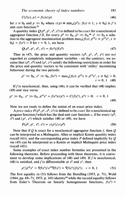
The economic theory of index numbers 1 8 1

C(f(x), p ) = f(x)c(p) (46)

for x � ON and p >> ON where c(p) � minx{prx: f(x) � 1 , x � ON} is f's unit cost function.21

A quantity index Q(p0, p1 , x0, x1) is defined to be exact for a neoclassical aggregator function f if, for every p0 >> ON, p1 >> ON, 22 xr >> ON a solu­tion to the aggregator maximization problem max.r{f(x): prrx ::5 prrxr, x � ON} = f(xr) > 0 for r = 0, l , we have

(47)

Thus in (47) , the price and quantity vectors (p0, p1 , x0, x1) are not regarded as completely independent variables - on the contrary, we as­sume that (p0, x0) and (p1, x1) satisfy the following restrictions in order for the price and quantity vectors to be consistent with 'utility' maximizing behaviour during the two periods:

pr >> ON, xr >> ON, f(xr) = maxx{flx): prTx ::5 prTxr, x � ON} > 0; r = 0, 1 (48)

Iff is neoclassical , then, using (46), it can be verified that (48) implies (49) and vice versa:

pr >> ON, xr >> ON, prTXr = f(xr)c(pr) = C(f(xr) , pr) > O; r = 0, 1

Now we are ready to define the notion of an exact price index.

(49)

A price index P(p0, p1 , x0, x1) is defined to be exact for a neoclassical ag­gregator function! which has the dual unit cost function c, if for every (p0, xO) and (p1 , x1) which satisfies (48) or (49) , we have

P(p0, p1 , xO, x1) = c(p1)/c(p0) (50)

Note that if Q is exact for a neoclassical aggregator function f, then Q can be interpreted as a Malmquist, Allen or implicit Koniis quantity index (recall (4 1)), and the corresponding price index P defined implicitly by Q via (45) can be interpreted as a Koniis or implicit Malmquist price index (recall (42)).

Some examples of exact index number formulae are presented in the following theorems. Before proceeding with these theorems, it is conve­nient to develop some implications of (48) and (49). If f is neoclassical, ( 48) is satisfied, and f is differentiable at xO and x1 , then

pr/prTxr = Vf(xr)/xrTVJ(xr) = Vf(xr)/f(xr) ; r = 0, 1 (51)

The first equality in (5 1 ) follows from the Hotelling ( 1935, p . 71 ) , Wold ( 1944, pp. 69-7 1 ; 1953, p. 145) identity23 while the second equality follows from Euler's Theorem on linearly homogeneous functions, f(xr) =

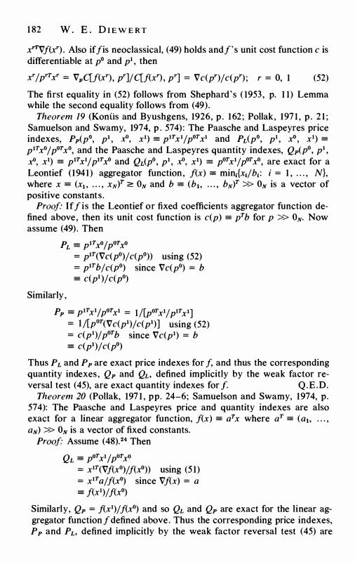
1 82 W . E . D I E W E RT

xr'I'Vf(xr) . Also iffis neoclassical, (49) holds and f's unit cost function c is differentiable at p0 and p1 , then

xr/prTxr = Vpqf(xr), pr]/qf(xr) , pr] = Vc(pr)/c(pr) ; r = 0, 1 (52)

The first equality in (52) follows from Shephard's ( 1953, p. 1 1) Lemma while the second equality follows from (49).

Theorem 19 (Koniis and Byushgens, 1926, p . 162; Pollak, 197 1 , p . 2 1 ; Samuelson and Swamy, 1974, p . 574) : The Paasche and Laspeyres price indexes, Pp(p0, p1 , xO, x1) = p1rx1/p0Tx1 and PL(p0, p1 , x0 , x1) = p1Tx0/p0rx0, and the Paasche and Laspeyres quantity indexes, Qp(p0, p1 , xO, x1) = p1rx1/p1rxo and QL(p0, p1 , xO, x1) = p0Tx1/p0Tx0, are exact for a Leontief (1941) aggregator function, f(x) = min;{xi/b; : i = 1 , . . . , N}, where x = (xi . . . . , xNl <::: ON and b = (bi. . . . , bN)T >> ON is a vector of positive constants.

Proof· If f is the Leontief or fixed coefficients aggregator function de­fined above, then its unit cost function is c(p) = prb for p >> ON. Now assume (49) . Then

pL = P1rxo;porxo

Similarly ,

= p1T(Vc(p0)/ c(p0)) using (52) = p1Tb/c(p0) since Vc(p0) = b = c(pl)/c(po)

Pp = P1rx1;porx1 = l/[porx1/p1rx1] = 1/[p0r(Vc(p1)/c(p1)] using (52) = c(p1)/p0rb since Vc(p1) = b = c(pl)/c(po)

Thus PL and Pp are exact price indexes for f, and thus the corresponding quantity indexes, Qp and QL, defined implicitly by the weak factor re­versal test (45), are exact quantity indexes for f. Q.E.D.

Theorem 20 (Pollak, 197 1 , pp. 24-6; Samuelson and Swamy, 1974, p. 574): The Paasche and Laspeyres price and quantity indexes are also exact for a linear aggregator function, f(x) = arx where ar = (ai. . . . , aN) >> ON is a vector of fixed constants.

Proof" Assume (48).24 Then

QL = Porx1;porxo = x1T(Vf(x0)/f(x0)) using (5 1) = x1ra/f(x0) since Vf(x) = a = f(x1)/f(x0)

Similarly, Qp = f(x1)/f(x0) and so QL and Qp are exact for the linear ag­gregator function f defined above. Thus the corresponding price indexes, Pp and PL, defined implicitly by the weak factor reversal test (45) are

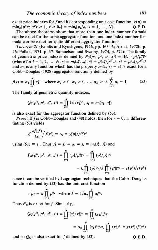
The economic theory of index numbers 1 83

exact price indexes for f and its corresponding unit cost function, c(p) = minx{prx: arx 2: 1 , x 2: ON} = min1{pi/a1 : i = 1 , . . . , N}. Q.E.D.

The above theorems show that more than one index number formula can be exact for the same aggregator function, and one index number for­mula can be exact for quite different aggregator functions.

Theorem 21 (Koniis and Byushgens, 1926, pp. 163-6; Afriat , 1972b, p. 46; Pollak, 197 1 , p. 37; Samuelson and Swamy, 1974, p. 574) : The family of geometric price indexes defined by p G(p0' p1 ' x0' X1) = rrr=l (pl/ PY)"' ( h '-' · - 1 2 N - ( o ) o - o o; or . .o 1 - 1 1/ lT 1 w ere �or 1 - , , • • • , , s1 = m; s; , s1 , s1 = P1X; p -"'- , s1 = P1X; p x and m1 is any function which has the property m;(s , s) = s) is exact for a Cobb-Douglas ( 1928) aggregator function f defined by

N N f(x) = a0 IT x'f' where a0 > 0, a1 > 0, . . . , aN > 0, L a1 = (53)

i=l i=l The family of geometric quantity indexes,

N QG(p0, p1 , x0, x1) = IT (xl/x?)"' , S; = m;(s?, sD

i=l is also exact for the aggregator function defined by (53).

Proof· Iffis Cobb-Douglas and (48) holds, then for r = 0, 1 , differen­tiating (53) yields

af(xr)I x[ � f(xr) = a; = x[p[ / PrT xr

using (5 1) = sj. Thus s? = sl = a; = s1 = m;(sf, sl) and N N

p G(P0' P1 ' _xO' x1) = TI (p}/ PY)"' = n (pV p�)"' i=l i=l

N N = k IT (p1)"'/k IT (pY)"i = c(p1)/c(p0)

i=l i=l

since it can be verified by Lagrangian techniques that the Cobb-Douglas function defined by (53) has the unit cost function

N N c(p) = k IT P�' where k = 1/a0 IT a1"1•

i=l i=l Thus PG is exact for f Similarly,

N N QG(po, p1, xo, xl) = IT (x}fxV"' = IT (xVx�)"'

i=l i=l N N

= ao IT (xl)"1/ao IT (xf)"' = f(x1)/f(x0) i=l i=l

and so QG is also exact for f defined by (53) . Q.E .D.

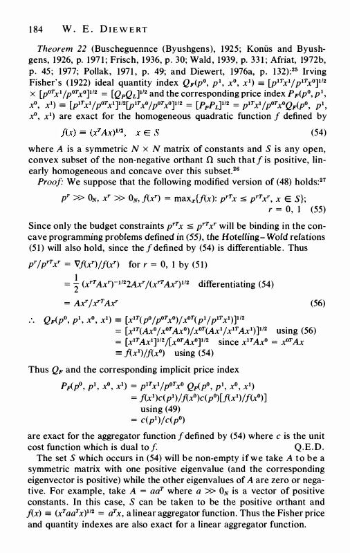
1 84 W . E . D I E W E RT

Theorem 22 (Buscheguennce (Byushgens), 1925; Koniis and Byush­gens, 1926, p. 197 1 ; Frisch, 1936, p . 30; Wald, 1939, p. 33 1 ; Afriat, 1972b, p. 45 ; 1977; Pollak, 1971 , p. 49; and Diewert, 1976a, p. 1 32):25 Irving Fisher' s ( 1922) ideal quantity index QF(p0, p1 , x0, x1) = (p1Tx1/p1rx0]1'2 x [p0rx1 /p0rx0]112 = [QpQL]112 and the corresponding price index PF(p0, p1 , xo, xl) = (plTxl/pOTxl]ll2(plTxO/pOTxO]ll2 = [PpPL]ll2 = plTxl/pOTxOQF(Po, pl , xO, x1) are exact for the homogeneous quadratic function f defined by

(54)

where A is a symmetric N x N matrix of constants and S is any open, convex subset of the non-negative orthant n such that f is positive, lin­early homogeneous and concave over this subset.26

Proof· We suppose that the following modified version of (48) holds:27 pr >> ON, xr >> ON, f(xr) = max,r{f(x): prTx ::S prTxr, x E S};

r = 0, 1 (55)

Since only the budget constraints prr x ::S prr xr will be binding in the con­cave programming problems defined in (55), the Hotelling- Wold relations (5 1 ) will also hold, since the f defined by (54) is differentiable . Thus pr/prTxr = Vf(xr)/f(xr) for r = 0, 1 by (5 1)

1 = - (xrr Axr)-1122Axr /(xrT Axr)112 differentiating (54) 2 = Axr / xrT Axr

. . QF(po, p1 , xo, xl) = [xlT(pO/pOTxO)/xOT(pl/p1Txl)]ll2 (56)

= [x1T(Ax0 / x0r Ax0)/ x0T(Ax1 / x1r Ax1)]112 using (56) = [xlTAxl]ll2/[x0TAx0]112 since xlTAxO = xOTAx = /(x1)//(x0) using (54)

Thus QF and the corresponding implicit price index

PF(po, p1 , xo, xl) = p1rx1/porxo QF(po, p1, xo, xl) = /(xl )c(pl) / /(xO)c(po)[/(x1) I f(xo)]

using (49) = c(pl)/c(po)

are exact for the aggregator function f defined by (54) where c is the unit cost function which is dual to f Q.E.D.

The set S which occurs in (54) will be non-empty if we take A to be a symmetric matrix with one positive eigenvalue (and the corresponding eigenvector is positive) while the other eigenvalues of A are zero or nega­tive. For example, take A = aar where a >> ON is a vector of positive constants . In this case, S can be taken to be the positive orthant and f(x) = (xraarx)112 = arx, a linear aggregator function. Thus the Fisher price and quantity indexes are also exact for a linear aggregator function.

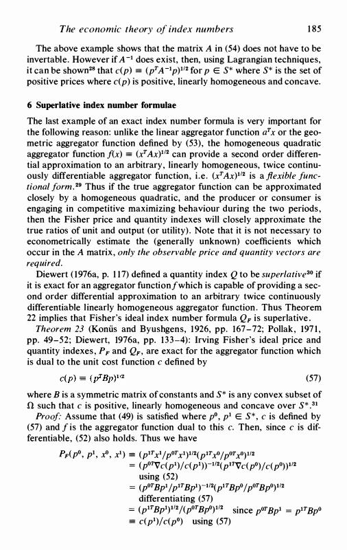
The economic theory of index numbers 1 85

The above example shows that the matrix A in (54) does not have to be invertable. However if A-1 does exist, then, using Lagrangian techniques, it can be shown28 that c(p) = (pr A-1p)112 for p E S* where S* is the set of positive prices where c(p) is positive, linearly homogeneous and concave.

6 Superlative index number formulae

The last example of an exact index number formula is very important for the following reason: unlike the linear aggregator function ar x or the geo­metric aggregator function defined by (53), the homogeneous quadratic aggregator function f(x) = (xr Ax)112 can provide a second order differen­tial approximation to an arbitrary, linearly homogeneous, twice continu­ously differentiable aggregator function, i .e. (xT Ax)112 is a flexible func­tional form. 29 Thus if the true aggregator function can be approximated closely by a homogeneous quadratic, and the producer or consumer is engaging in competitive maximizing behaviour during the two periods , then the Fisher price and quantity indexes will closely approximate the true ratios of unit and output (or utility) . Note that it is not necessary to econometrically estimate the (generally unknown) coefficients which occur in the A matrix, only the observable price and quantity vectors are required.

Diewert ( 1976a, p. 1 17) defined a quantity index Q to be superlative30 if it is exact for an aggregator functionfwhich is capable of providing a sec­ond order differential approximation to an arbitrary twice continuously differentiable linearly homogeneous aggregator function. Thus Theorem 22 implies that Fisher's ideal index number formula QF is superlative .

Theorem 23 (Koniis and Byushgens, 1926, pp. 167-72; Pollak, 197 1 , pp. 49-52; Diewert, 1976a, pp. 133-4) : Irving Fisher's ideal price and quantity indexes , PF and QF. are exact for the aggregator function which is dual to the unit cost function c defined by

(57)

where B is a symmetric matrix of constants and S* is any convex subset of n such that c is positive, linearly homogeneous and concave over S* .31

Proof· Assume that ( 49) is satisfied where p0, p1 E S*, c is defined by (57) and f is the aggregator function dual to this c. Then, since c is dif­ferentiable, (52) also holds. Thus we have

PF(po, p1 , xo, xi ) = (p1rx1/porx1)112(p1Txo/porxo)112 = (po1V c(pl)/ c(p1))-112(p11V c(po)/ c(po))112

using (52) = (pOTBpl / p1TBpl)-112(plTBpo / poTBpo)112

differentiating (57) = (p1rBp1)112 /(porBpo)112 since PoTBp1 = P1TBpo = c(p1)/c(p0) using (57)

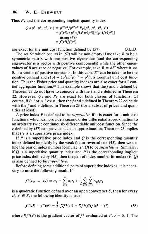
1 86 W . E . D I E W E RT

Thus PF and the corresponding implicit quantity index

QF(po, p1 , xo, xi ) = p1rx1/porxo PF(po, p1 , xo, xi ) = f(x1)c(pl)/f(xO)c(po)[c(p1)/ c(po)]

using (49) = f(x1)/f(x0)

are exact for the unit cost function defined by (57). Q.E.D. The set S* which occurs in (57) will be non-empty if we take B to be a

symmetric matrix with one positive eigenvalue (and the corresponding eigenvector is a vector with positive components) while the other eigen­values of B are zero or negative. For example, take B = bF where b >> ON is a vector of positive constants . In this case, S* can be taken to be the positive orthant and c(p) = (prbbrp)112 = prb, a Leontief unit cost func­tion. Thus the Fisher price and quantity indexes are also exact for a Leon­tief aggregator function. 32 This example shows that the f and c defined by Theorem 23 do not have to coincide with the f and c defined in Theorem 22. However, QF and PF are exact for both classes of functions. Of course, if B-1 or A-1 exist, then thef and c defined in Theorem 22 coincide with the f and c defined in Theorem 23 (for a subset of prices and quan­tities at least) .

A price index P is defined to be superlative if it is exact for a unit cost function c which can provide a second order differential approximation to an arbitrary twice continuously differentiable unit cost function. Since the c defined by (57) can provide such an approximation, Theorem 23 implies that PF is a superlative price index.

If P is a superlative price index and Q is the corresponding quantity index defined implicitly by the weak factor reversal test (45), then we de­fine the pair of index number formulae (P, Q) to be superlative . Similarly , if Q is a superlative quantity index and f> is the corresponding implicit price index defined by (45), then the pair of index number formulae (f>, Q) is also defined to be superlative.

Before defining some additional pairs of superlative indexes, it is neces­sary to note the following result. If

N } N N f*(zi . . . . , ZN) = a0 + L a1z1 + 2 L L ai.iz1z;

i=I i=I j=I is a quadratic function defined over an open convex set S, then for every z0, z1 E S, the following identity is true:

(58)

where Vf*(zr) is the gradient vector off* evaluated at zr, r = 0, 1 . The

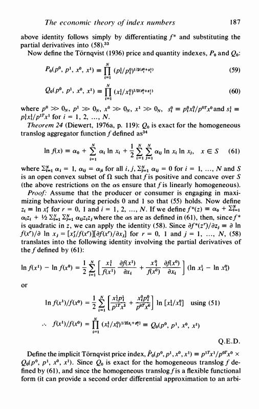
The economic theory of index numbers 1 87

above identity follows simply by differentiating f* and substituting the partial derivatives into (58).33

Now define the Tornqvist ( 1936) price and quantity indexes, P0 and Qo: N p o(Po' p1 ' xO' xl) = IT (pl/ p?)ll2<b"f+•P (59) i=l N

Qo(po, p1 , xO, xl) = IT (xl/x?)112<b"f+•p (60) i=l

where p0 >> ON, p1 >> ON, x0 >> ON, x1 >> ON, s? = pfxY/p0Tx0 and sf = pfxl/p1rx1 for i = 1 , 2, . . . , N.

Theorem 24 (Diewert, 1976a, p. 1 19): Q0 is exact for the homogeneous translog aggregator function f defined as34

N 1 N N In f(x) = ao + L a; In X; + 2 L L au In x; In XJ. x E S (61)

i=l i=l J=l

where }:.r=1 a; = 1, au = a1; for all i, j, }:.f=,1 au = 0 for i = 1, . . . , N and S is an open convex subset of n such that f is positive and concave over S (the above restrictions on the as ensure that f is linearly homogeneous).

Proof· Assume that the producer or consumer is engaging in maxi­mizing behaviour during periods 0 and 1 so that (55) holds. Now define z; = ln xf for r = 0, 1 and i = l , 2, . . . , N. If we definef*(z) = a0 + Lr=1 a;z; + Y2 }:.�1 Lf=,1 auz;z1 where the as are as defined in (61) , then, sincef* is quadratic in z , we can apply the identity (58). Since af*(zr)/oz1 = a In f(xr)/a In x1 = [xj/f(xr)][af(xr)/ax1] for r = 0, 1 and j = 1 , . . . , N, (58) translates into the following identity involving the partial derivatives of the f defined by (61):

1 N [ Xf of(X1) X� ofix0) ] In f(x1) - In f(x0) = 2 � f(x1) --ax;- + fixO) ax;- (In x� - In Xl) or

1 N [x1pl XQpO ] ln f(x1)/f(x0) = 2 L :r \ + ;r;o In [xUXl] using (5 1) i=l p x p

N . . f(xl)/f(xo) = IT (xt/xf) 112cs;+s'/l = Qo(po, p1, xo, xl)

i=l Q.E.D.

Define the implicit Tomqvist price index, F0(p0, p1 , xO, x1) = p1rx1 /porx0 x Q0(p0, p1, xO, x1) . Since Q0 is exact for the homogeneous translog f de­fined by (61) , and since the homogeneous translogfis a flexible functional form (it can provide a second order differential approximation to an arbi-

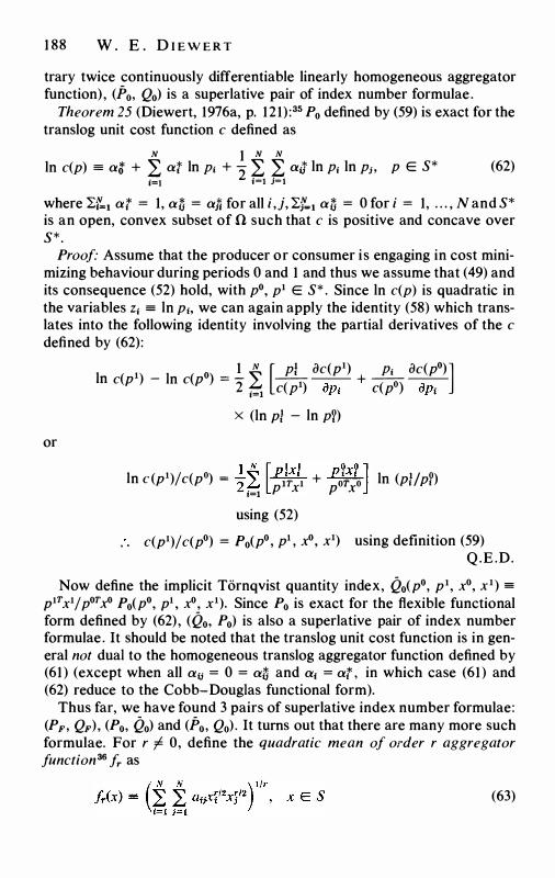
1 88 W . E . D I E W E R T

trary twice continuously differentiable linearly homogeneous aggregator function) , (F0, Q0) is a superlative pair of index number formulae.

Theorem 25 (Diewert, 1976a, p. 12 1) :35 P0 defined by (59) is exact for the translog unit cost function c defined as

N 1 N N In c(p) = at + ,L at In Pi + 2 ,L ,L aif In Pi In Ph p E S* (62)

i=l i=l J=l where �f..1 at = 1, at; = a1� for all i ,j, �f=1 at; = 0 for i = 1, . . . , N and S* is an open, convex subset of 0 such that c is positive and concave over S*.

Proof: Assume that the producer or consumer is engaging in cost mini­mizing behaviour during periods 0 and 1 and thus we assume that (49) and its consequence (52) hold, with p0, p1 E S* . Since In c(p) is quadratic in the variables zi = In p;, we can again apply the identity (58) which trans­lates into the following identity involving the partial derivatives of the c defined by (62):

or

1 0 _ 1 N [ Pl ac(p1) Pi ac(p0)] In c(p ) - In c(p ) - -2 ,L -( 1)

-,,-_ + -( o) -,,-_-i=l C P up, C p up,

x (In pl - In p?)

1 o _ ..!� [plxl p?x? J In c(p )/c(p ) - 2 £,,, lT 1 + or o In (plfp?) i=l p x p x

using (52)

. . c(p1)/c(p0) = P0(p0, p1 , x0, x1) using definition (59) Q.E .D.

Now define the implicit Tornqvist quantity index, Q0(p0, p1, x0, x1) = p1Tx1/p0Tx0 P0(p0, p1 , x0, x1). Since P0 is exact for the flexible functional form defined by (62) , (Q0, P0) is also a superlative pair of index number formulae. It should be noted that the translog unit cost function is in gen­eral not dual to the homogeneous translog aggregator function defined by (61 ) (except when all ail = 0 = at; and a1 = at , in which case (61 ) and (62) reduce to the Cobb-Douglas functional form).

Thus far, we have found 3 pairs of superlative index number formulae: (PF, QF), (P0, Q0) and (F0, Q0). It turns out that there are many more such formulae. For r f 0, define the quadratic mean of order r aggregator function36 fr as

(63)

The economic theory of index numbers 1 89

where S is an open subset of fl where fr is neoclassical , and define the quadratic mean order r unit cost function37 Cr as

Cr(P) = (� � bup�12p'j'2)"r, p E S* (64)

where S* is an open subset of fl where Cr is neoclassical . For r I- 0, define the following price and quantity indexes:

Pr(po, p1, xo, x1) = {� s?(p}/p7y12f'r {t1 s}(p}jp�)-rt2r1tr

Qr(Po' pl ' xO' xl) = {� sY(xl/ xYY'2} l/r { tl s}(x}/ �)-rt2 } -1/r (65)

where p0, p1 , x0, x1 >> ON, sf = pfxf!p0Tx0 and sf = pfx1/p1Tx1 for i = 1 , 2, . . . , N.

It can be shown38 (in a manner analogous to the proof of Theorem 22), that for each r I- 0, Qr defined by (65) is exact for fr defined by (63). Simi­larly , it can be shown39 (in a manner analogous to the proof of Theorem 23), that Pr defined by (65) is exact for Cr defined by (64) . Since it is easy to show (cf. Diewert, 1976a, p. 1 30) that fr and Cr are flexible functional forms for each r I- 0, if can be seen that (Pr, Qr) and (Pr, Qr) are pairs of superlative index number formulae for each r I- 0, where Qr = p1Tx1/p0TxOTPr and Pr = p1Tx1/p0Tx0Qr. Note that P2 = PF (Fisher's ideal price index) and Q2 = QF (Fisher's ideal quantity index), so that (P2 , Q2) = (P2, Q2) = (PF, QF). Moreover, it can be shown that the homoge­neous translog aggregator function defined by (61) is a limiting case of fr defined by (63) as r tends to zero (similarly, the translog unit cost func­tion defined by (62) is a limiting case of Cr as r tends to zero)40 and that Q0 defined by (60) is a limiting case of Qr as r tends to 0 while P0 de­fined by (59) is a limiting case of Pr as r tends to 0.41

Given such a multiplicity of superlative indexes, the question arises: which index number formula should be used in empirical applications? The answer appears to be that it doesn't matter, provided that the varia­tion in prices and quantities is not too great going from period 0 to period 1 . This is because it has been shown42 that the functions Pr and P8 dif­ferentially approximate each other to the second order for all r and s , pro­vided that the derivatives are evaluated at any point where p0 = p1 and xO = x1 : i .e. we have Pr(p0, p1 , xO, x1) = Ps(p0, p1 , x0, x1), 'i1Pr(p0, p1 , x0, x1) = 'i1Ps(p0, p1, x0, x1) and 'i12Pr(P0, p1 , x0, x1) = 'i12Ps{p0, p1 , x0, x1) for all r and s, provided that p0 = p1 >> ON . 'ilPr stands for the 4N dimensional vector of first order partials of Pr, 'i12Pr stands for the 4N matrix of second order partials of Pr, etc. The quantity indexes Qr and Q8 similarly differen­tially approximate each other to the second order for all r and s, provided

1 90 W . E . D I E W E RT

that prices and quantities are the same for the two periods . These results are established by straightforward but tedious calculations - moreover, the assumption of optimizing behaviour on the parts of the consumer or producer is not required in order to derive these results.

Diewert ( 1978b) also shows that the Paasche and Laspeyres price in­dexes, Pp and PL, differentially approximate each other and the superla­tive indexes, Pr and P., to the first order for all r and s, provided that prices and quantities are the same for the two periods . Thus if the varia­tion in prices and quantities is relatively small between the two periods, the indexes PL, Pp, Pr and i\ will all yield approximately the same answer.

Diewert ( 1978b) argues that the above results provide a reasonably strong justification for using the chain principle when calculating official indexes such as the consumer price index or the GNP deflator, rather than using a fixed base, since in using the chain principle the base is changed every year, and thus the changes between p0 and p1 and x0 and x1 will be minimized, leading to smaller discrepancies between PL and Pp, and even smaller discrepancies between the superlative indexes Pr and F8•43

However, in some situations (e .g. in cross country comparisons or when decennial census data are being used), there can be considerable variation in the price and quantity data going from period (or observation) 0 to period (or observation) 1 , in which case the indexes Pr and Ps can differ considerably. In this situation, it is sometimes useful to compare the variation in the N quantity ratios (x}/ xf) to the variation in the N price ratios (p}/pf). If there is less variation in the quantity ratios than in the price ratios , then the quantity indexes Qr defined by (66) are share weighted averages of the quantity ratios and will tend to be more stable than the implicit indexes Qr. On the other hand, if there is less variation in the price ratios than in the quantity ratios (the more typical case), then the price indexes Pr defined by (65) are share weighted averages of the price ratios (p}/ pf) and will tend to be in closer agreement with each other than the implicit price indexes Pr. Thus, in the first situation, we would recom­mend the use of (Fr, Qr) for some r,44 while in the second situation we would recommend the use of (Pr, Qr) for some r.45 Notice that the Fisher index, (PF, QF) = (P2, Q2) = (F2, Q2) can be used in either situation. A further advantage for the Fisher formulae (PF, QF) is that QF is consistent with revealed preference theory: i .e . , even if the true aggregator function f is non-homothetic, under the assumption of maximizing behaviour, QF will correctly indicate the direction of change in the aggregate when re­vealed preference theory tells us that the aggregate is decreasing, increas­ing or remaining constant (cf. Diewert, 1976a, p. 1 37) . Recall also that QF is consistent both with a linear aggregator function (perfect substitutabil­ity) and a Leontief aggregator function (no substitutability). No other su-

The economic theory of index numbers 1 9 1 perlative index number formula Qr or Qr, r "I 2 , has the above rather nice properties.

We conclude this section by showing that some of the above superlative index number formulae are also exact for non-homothetic aggregator functions .

Theorem 26 (Diewert, 1976a, p . 122): Let the functional form for the cost function C(u, p) be a general translog defined by

N 1 N N In C(u, p) = ao + L ai In Pi + 2 L L Yu In Pi In PJ

i=l l=l j=l N I

+ 80 In u + L 81 In p; In u + 2 e0(ln u)2 (66) l=l

where the parameters satisfy the following restrictions : N N L a; = I ; 'Y1J = "/Ji for all i, j; L Yu = 0 i=l j=l N

for i = 1 , 2, . . . , N, and L 81 = 0 (67) i=l

Let (u0, p0) and (u1, p1) belong to a (u, p) region where C(u, p) satisfies Conditions II where u0 > 0, u1 > 0, p0 >> ON, p1 >> ON and the corre­sponding quantity vectors are x0 = VpC(u0, p0) > ON and x1 = VpC(u1 , p1) > ON respectively. Then

(68) where Po is the Tornqvist price index defined by (59) and the reference utility level u* = (u0 u1)112•

Proof: For a fixed u*, In C(u* , p) is quadratic in the variables zi = In p1 and thus we may apply the identity (53) to obtain

In C(u*, p1) - In C(u* , p0) 1 N

= 2 � [pf ln C(u* , p1)/<Jp; 1=1

+ pf In C(u* ' p0)/ api][ln pf - ln pf] I N

= 2 L [pl a ln C(u1 , p1)/<Jp; i=l

+ pf a ln C(u0 ' p0)/ api][ln Pl - In pf]

where the equality follows upon evaluating the derivatives of C and noting that 2 In u* = In u1 + In u0

= ln P0(p0, p1, xO, x1) using the definitions of xO, x1 and P0 and equations (52). Q.E.D.

1 92 W . E . D I E W E RT

Note that the right hand side of (68) is the true Koniis price index which corresponds to the general translog cost function defined by (66) , evalu­ated at the reference utility level u*, the square root of the product of the period 0 and 1 utility levels, u0 and u1 • We note that the translog cost func­tion can provide a second order differential approximation to an arbitrary twice continuously differentiable cost function.

Theorem 27 (Diewert, 1976a, pp. 123-4) : Let the aggregator function F be such that F's distance function D is the translog distance function de­fined by In D(u, x) = In C(u, x) where C is defined by (66) and (67). Let (u0, x0) and (u1 , x1) belong to a (u , x) region where D(u , x) satisfies Condi­tions IV where u0 > 0, u1 > 0, x0 >> ON, x1 >> ON, D(u0, x0) = 1 , D(u1 , x1) = 1 and the corresponding vectors of normalized prices are p0 / p0T x0 = VxD(u0, xO) > ON and p1/p1rx1 = VxD(u1 , x1) > ON respectively.46 Then

(69)

where Q0 is the Tornqvist quantity index defined by (60) and the reference utility level u* = (u0 u1 )112 .

Proof· For a fixed u*, In D(u* , x) is quadratic in the variables z1 = In x1 and thus we may apply the identity (58) to obtain

In D(u* , x1) - In D(u* , xO) 1 N

= 2 2 [x} a In D(u*, x1)/iJx1 i=l

+ xf a In D(u*, xO)/iJx1][ln xl - In xf]

1 N = 2 2 [x} In D(u1, x1)/iJx1

i=l + xf a In D(u0, xO)/iJx;] In (xt/xf)

where the equality follows upon evaluating the derivatives of D and noting that 2 In u* = In u1 + In u0 1 N

= 2 2 [x} plf p1rx1D(u1 , xl) i=l

+ xfpYfp0TxOD(u0, xO)] In (xt/xf) using pr/prTxr = Vx D(ur, xr), r = 0, 147

= In Qo(Po, p1, xo, xl)

using D(u1, x1) = 1 , D(u0, x0) = 1 and the definition of Q0• Q.E.D.

Note that the right hand side of (69) is the Malmquist quantity index which corresponds to the translog distance function, evaluated at the ref­erence utility level u* = (u u1)112 • Theorem 27 provides a fairly strongjus-

The economic theory of index numbers 193

tification for the use of Q0 in empirical applications, since the translog dis­tance function can differentially approximate an arbitrary twice continu­ously differentiable distance function to the second order. 48 However, the Fisher ideal index Q2 can be given a similar strong justification in the con­text of non-homothetic aggregator functions.49

7 Historical notes and additional related topics

Our survey of the economic theory of index numbers is based on the work of Koniis (1924), Frisch (1936), Allen (1949) , Malmquist ( 1953), Pollak ( 1971) , Afriat ( 1972; 1977) and Samuelson and Swamy (1974). The results noted in sections 2 and 3 are either taken directly from or are straightfor­ward modifications of results obtained by the above authors, except that in many cases we have weakened the original author's regularity condi­tions.50

The reader will have noted that many of the proofs in sections 2 and 3 use arguments that are used in revealed preference theory. For further material on the interconnections between revealed preference theory and index number theory, see Leontief (1936), Samuelson ( 1947, pp. 146-63), Allen (1949), Diewert (1976b), Vartia (1976b, p. 144) and Afriat ( 1977).

There is an extensive literature on the measurement of real output or real value added that is analogous to our discussion on the measurement of utility or real input: see Samuelson ( 1950), Bergson (1961), Moorsteen ( 1961), Fisher and Shell ( 1972, pp. 49- 1 13) (the last 3 references make use of a quantity index analogous to the Malmquist index), Samuelson and Swamy ( 1974, pp. 588-92), Sato (1976b), Archibald (1977) and Diewert (1980).

Background material on the duality between cost, production or utility, and distance or deflation functions can be found in Shephard ( 1953; 1970), McFadden (1978), Hanoch (1978), Blackorby, Primont and Russell ( 1978), Diewert (1974a; 1978c), Deaton (1979) and Weymark (1978).

Turning now to sections 5 and 6, for theorems which prove converses to Theorems 19 to 25 under various regularity conditions, see Byushgens (1925), Koniis and Byushgens (1926), Pollak (1971) , Diewert ( 1976a) and Lau (1979).

Sato (1976a) shows that a certain index number formula (which was de­fined independently by Vartia (1974)) is exact for the CES aggregator function defined by (63) with av = 0 for i I- j for all r, while Lau (1979) develops a partial converse theorem.

In Theorem 22, preferences were assumed to be represented by the transformed quadratic function, (xT Ax)112 • The assumption that prefer­ences can be represented, at least locally, by a general quadratic function of the form a0 + aT x + Yur Ax has a long history in economics, perhaps

1 94 W . E . D I E W E RT

starting with Bennet (1920). Other authors who have approximated pref­erences quadratically, in addition to those mentioned in Theorem 22, in­clude Bowley (1928), Hotelling ( 1938), Hicks (1946, pp. 33 1 -3), Kloek (1967), Theil ( 1967, pp. 200- 12; 1968), and Harberger ( 1971) .

Kloek and Theil utilize quadratic approximations in the logarithms of prices and quantities and they obtain results which are related to Theorems 25 and 26 above. Kloek ( 1967) shows that the Tornqvist price index P0(p0, p1, x0, x1) approximates the true Koniis price index PK(p0, p1 , um) to the second order where um, an intermediate utility level, is defined implicitly by the equation C(um, p0)/C(u0, p0) = C(u1, p1)/C(um, p1) and C is the true cost function. On the quantity side, Kloek ( 1967) shows that the implicit Tornqvist quantity index (lo(p0, p1, x0, x1) approximates the true Allen quantity index QA(xO, x1, pm) = C[F(x1), pm]/C[F(x0), pm] to the sec-ond order where pm = (p'{', p-;,', . . . , p'Jlf, an intermediate price vector, is defined by p'{' = (pf pl )112, i = 1 , . . . , N and F is the aggregator function dual to the true cost function C. On the other hand, Theil ( 1968) shows that P0(p0, p1 , x0, x1) approximates the true Koniis price index PK(p0, p1 , u) to the second order where u, an intermediate utility level, is defined as u = G(pm /ym) where G is the indirect utility function dual to the true cost function C,51 pm is Kloek's intermediate price vector defined above and ym = (p0r x0p1r x1)112 is an intermediate expenditure . Finally, on the quan­tity side, Theil ( 1967; 1968) proves Kloek's result (i.e. that Q0(p0, p1 , x0, x1) approximates QA (x0, x1 , pm) to the second order) and in addition , shows that the direct Tornqvist quantity index Q0(p0, p1 , xO, x1) also approximates QA(xO, x1 , pm) to the second order.

It should be noted that index number theory and consumer surplus analysis are closely related. Thus the Paasche-Allen quantity index QA(x0, x1 , p1) = C(F(x1), p1]/ C[F(x0), p1], is closely related to Hicks' ( 1941 -42, p. 128; 1946, pp. 40- 1) compensating variation in income, 52 C[F(x1), p1] - C[F(xO), p1], and the Laspeyres-Allen quantity index, QA(x0, x1, p0) = C[F(x1) , p0]/C[F(x0) , p0], is closely related to Hicks' ( 194 1 -42, p. 128; 1946, p. 331) equivalent variation in income, C[F(x1) , p0] - C[F(xO) , p0]. Thus the various bounds we developed for index numbers in the previous section have counterparts in consumer surplus analysis. Hicks ( 194 1 -42) and Samuelson ( 1947, pp. 189-202) emphasized the in­terconnection between index number theory and consumer surplus mea­sures. For additional results and references to the literature on consumer surplus, see Hotelling ( 1938), Samuelson ( 1942), Harberger ( 1971) , Silber­berg ( 1972), Hause (1975), Chipman and Moore ( 1976) and Diewert (1976b) . The attractiveness of the Malmquist quantity index Q,v(x0, x1, x) does not seem to have been noted in the applied welfare economics litera­ture, although the closely related concept inherent in Debreu's ( 1951) coefficient of resource utilization has been recognized. Perhaps in the fu-

The economic theory of index n umbers 1 95

ture there will be more applications of the Kloek-Theil approximation re­sults, or of Theorem 27 above which shows that the Tornqvist quantity index Q0 is numerically equal to a certain Malmquist index.

Another type of price and quantity index which we must mention is the Divisia ( 1925; 1926, p. 40) index, (which is perhaps due to Bennet ( 1920, p. 461)) . The Bennet-Divisia justification for these indexes proceeds as follows. Regard (xi . . . . , xNf = x and (Pi . . . . , PN)T = p as functions of time, x(t) and p(t) for i = 1 , . . . , N. Now differentiate expenditure with respect to time and we obtain:53

a [� P1(t)x1(t) ]/at = t1 P1U)ax1(t)/at + �1 x1(t)ap1(t)/at (70)

Now divide both sides of the above equation through by �f'..1 p,(t)x,(t) = p(tf x(t) and we obtain the identity:

N a In fp(tfx(t)]/at = Lslt)a In x1(t)/at

1=1 N + L s1(t)a In P1U)/at (71)

i=l where s1(t) = p1(t)x1(t)/p(t)Tx(t) for i = 1 , 2, . . . , N. The term on the left hand side of (70) is the rate of change of expenditures, which is decom­posed into a share weighted rate of change of quantities plus a share weighted rate of change of prices. Denote x1(t) = axi(t)/ at and p1(t) = ap1(t)/at and integrate both sides of (70) to obtain

In p(l)Tx(l)/p(Ofx(O) = {1 [� si(t)x1(t)/x1(t)] dt

+ J: [� s,(t)p1(t)/p1(t) ]dt (72)

The first term on the right hand side of the above equation is defined to be the natural logarithm of the Divisia quantity index, In [X(l)/X(O)], while the second term is the logarithm of the Divisia price index, ln [P( l)/ P(O)].

The above derivation of the Divisia indexes, X(l )/X(O) and P(l )/ P(O), is devoid of any economic interpretaton. However, Ville ( 195 1) , Malmquist ( 1953 , p. 227), Wold ( 1953 , pp. 134-47), Solow ( 1957), Gorman ( 1959, p. 479; 1970), Jorgenson and Griliches ( 1967, p. 253) and Hulten ( 1973) show that if the consumer or producer is continuously maximizing a well be­haved linearly homogeneous aggregator function subject to a budget con­straint between t = 0 and t = 1 , then P(l)/ P(O) = PK{p(O) , p(l) , x) (i.e. the Divisia price index equals the true Koniis price index for any reference quantity vector x >> ON) and we can deduce that X(l)/ X(O) = Q�x(O) , x( l ) , x) = �(x(O) , x( l ) , p) = QK{p(O) , p(l ) , x(O) , x( l ) , x) (i.e. the Divisia

1 96 W . E . D I E W E RT

quantity index equals the Malmquist, Allen, and implicit Koniis quantity indexes for all reference vectors x >> ON and p >> ON) . On the other hand, Ville ( 195 1 , p. 127), Malmquist ( 1953, pp. 226-7), Gorman ( 1970, p. 7) , Silberberg ( 1972, p. 944) and Hulten ( 1973, pp. 102 1 -2) show that if the aggregator function is not homothetic , then the line integrals defined on the right hand side of (72) are not independent of the path of integration and thus the Divisia indexes are also path dependent.

We have not stressed the Divisia approach to index numbers in this survey since economic data typically are not collected on a continuous time basis. Since there are many ways of approximating the line integrals in (72) using discrete data points, the Divisia approach to index number theory does not significantly narrow down the range of discrete type index number formulae, P(p0 , p1 , x0, x1) and Q(p0, p1 , x0, x1) , that are consistent with the Divisia approach.

The line integral approach also occurs in consumer surplus analysis: see Samuelson ( 1942; 1947, pp. 189-202), Silberberg ( 1972), Rader ( 1976) and Chipman and Moore ( 1976).

Divisia indexes and exact index number formulae also play a key role in another area of economics which has a vast literature, namely the mea­surement of total factor productivity . A few references to this literature are Solow (1957), Domar (1961) , Richter ( 1966), Jorgenson and Griliches ( 1967; 1972), Gorman (1970), Ohta ( 1974), Star ( 1974) , Usher ( 1974), Christensen, Cummings and Jorgenson ( 1980), Diewert ( 1976a, pp. 124-9; 1980, pp. 487-98) and Allen ( 1978). To see the relationship of this literature to superlative index number formulae, consider the following example : Let ur = f(xr) > 0, r = 0, 1 be ' intermediate' output produced by a competitive (in input markets) cost minimizing firm where xr >> ON is a vector of inputs utilized during period r, and f is the homogeneous translog production function defined by (61) . Letting w0 >> ON and w1 >> ON be the vectors of input prices the producer faces during periods 0 and 1 , Theorem 24 tells us that

(73)

where Q0 is the Tornqvist quantity index defined by (60). Using (49) , we also have

(74)

where c(w) is the unit cost function which is dual to f(x) . Suppose now that 'final' output is yr = arf(xr) , r = 0, 1 where ar > 0 is defined to be a technology index for period r. The ratio a1 / a0 can be defined to be a mea­sure of Hicks neutral technical progress.54 Using (73),

The economic theory of index numbers 1 97

Thus a1 / a0 can be calculated using observable data. 55 The unit cost func­tion for y in period r is c(w)/ar. Now suppose the producer behaves monopolistically on his output market and sells his period r output yr at a price pr equal to unit cost times a markup factor mr > 0, i .e .

pr = mrc(wr)/ar, r = 0, 1

Using (76),

(76)

m1 I mo = [pl I po][a1 I ao]/[c(wl)/ c(wo)] = [p1yo / poyo]/[w1r x1 /worxo] (77)

using (74) and (75). Thus the rate of markup change m1/m0 can be calcu­lated by (77) , the value of output ratio deflated by the value of inputs ratio, using observable data. 56 However, if pure profits are zero in each period, then pryr = wrTxr = [mr c(wr)/ar][arf(xr)] (using (76)) = mrwrTxr (using (74)) so that mr = 1 for r = 0, 1 .

Another area of research which somewhat surprisingly is closely re­lated to index number theory is the measurement of inequality: see Black­orby and Donaldson (1978; 1980; 1981) .

Typically , a price or quantity index is not constructed in a single step. For example, in constructing a cost of living index, first food, clothing, transportation and other sub-indexes are constructed and then they are combined to form a single cost of living index. Vartia ( 1974, pp. 39-42; 1976a, p. 124; 1976b, pp. 84-9) defines an index number formula P(p0, p1 , x0, x1) to be consistent in aggregation if the numerical value of the index constructed in two (or more) stages necessarily coincides with the value of the index calculated in a single stage. Vartia ( 1976b; p . 90) stresses the importance of the consistency in aggregation property for na­tional income accounting and notes that the Paasche and Laspeyres in­dexes have this property (as do the geometric indexes PG and QG defined in Theorem 2 1 above). Vartia ( 1976b, pp. 1 2 1 -40) exhibits many other index number formulae that are consistent in aggregation. Unfortunately , the two families of superlative indexes, (Pr. Qr) and (F8, Q8) , are not con­sistent in aggregation for any r or s . However, Diewert ( 1978b) using some of Vartia's results shows that the superlative indexes are approximately consistent in aggregation (to the second order in a certain sense). Addi­tional results are contained in Blackorby and Primont ( 1980) . Related to the consistency in aggregation property for an index number formula are the following issues which have been considered by Pollak ( 1975) , Pri­mont ( 1977), Blackorby and Russell ( 1978) and Blackorby, Primont and Russell ( 1978, chapter 9): (i) under what conditions do well defined Koniis cost of living sub-indexes exist for a subset of the commodity space and (ii) under what conditions can the sub-indexes be combined into the true overall Koniis cost of living index Px? Finally , a related result is due to Gorman (1970, p. 3) who shows that the line integral Divisia indexes de-

1 98 W . E . D I E W E RT

fined above 'aggregate conformably' or are consistent in aggregation, to use Vartia' s term.

If we are given more than two price and quantity observations, then some ideas due to Afriat (1967) can be utilized in order to construct non-parametric index numbers. Let there be I given price-quantity vectors (pi, xi) where pi >> ON, xi > ON, i = 1 , 2, . . . , I. Use the given data in order to define Afriat's ijth cross coefficient, Du = (piTxi/piTxi) - 1 for 1 :::; i, j :::; /. Now consider the following linear programming problem in the 2/ + 212 variables >..1, cf>i. s�, sij, i, j = 1 , . . . , I:

I I minimize L L sij subject to

i=l j=l (i) >..;Du = cf>1 - cf>; + s� - sij ; 1 , 1 = 1 , 2, . . . , I, (ii) A; ;:::: 1 ; i = 1 , 2, . . . , I, and (iii) cf>; ;:::: 0, s� ;:::: 0, sij ;:::: 0; i, j = 1 , 2, . . . , I

Diewert (1973)57 shows that if x1 is a solution to

max.r{F(x): p;rx :::; p;rx;, x ;:::: ON}

(78)

(79)

for i = 1 , 2, . . . , I where F is a continuous from above aggregator function which is subject to local non-satiation (so that the budget constraint p1rx :::; p1Txi will always hold as an equality for an x which maximizes F(x) subject to the budget constraint) , then the objective function in the pro­gramming problem (78) will attain its lower bound of zero. On the other hand, Afriat ( 1967) shows that if the objective function in (78) attains its lower bound of 0 so that >..t Du ;:::: cf>f - cf>t for all i and j where >..t , cf>t denote solution variables to (78), then the given quantity vector x1 is a so­lution to the utility maximization problem (79) for i = 1 , 2, . . . , I. More­over, Afriat ( 1967, pp. 73-4) shows that a utility function F* which is con­sistent with the given data in the sense that F*(x1) = max.r{F*(x): pirx :::; p1rx1 ; x ;:::: ON} for i = 1 , 2, . . . , I can be defined as F*(x) = min1{Ft(x) : i = 1 , . . . , l} where

(80)

where the number cf>t and >..t are taken from the solution to (78). Afriat notes that this F* is continuous, increasing and concave over the non­negative orthant and that F*(x1) = cf>t for i = 1 , . . . , I. Thus if the observed data are consistent with a decision maker maximizing a continuous from above, locally non-satiated aggregator function F(x) subject to I budget constraints , then the solution to the linear programming problem (78) can be used in order to construct an approximation F* to the true F, and this F* will satisfy much stronger regularity conditions. Diewert ( 1973, p. 424) notes that we can test whether the given data are consistent with the addi-

The economic theory of index numbers 1 99

tional hypothesis that the true aggregator function is homothetic or lin­early homogeneous by adding the following restrictions to (78): (iv) A.1 = cf>i. I = I , . . . , I. Geometrically , these additional restrictions force all of the hyperplanes defined by (61) through the origin: i .e . Ft(ON) = 0 for all i. Once the linear program (78) is solved, either with or without the addi­tional normalizations (iv), we can calculate F*(xi) = cf>t for all i and thus the quantity indexes F*(xi+1)/ F*(x1) can readily be calculated. Diewert and Parkan ( 1978) calculated these non-parametric quantity indexes using some Canadian time series data58 and compared them with the superlative indexes Q2, Q0 and Q0• The differences between all of these indexes turned out to be small.59 The above method for constructing parametric indexes is of course closely related to revealed preference theory.

Finally , we mention that there is an analogous 'revealed production theory' which allows one to construct non-parametric index numbers and non-parametric approximations to production functions and production possibility sets by solving various linear programming problems:60 see Farrell ( 1957), Afriat (1972a) , Hanoch and Rothschild (1972) and Diewert and Parkan (1979).

Notes

University of British Columbia, Vancouver, Canada. The financial support of the Canada Council is gratefully acknowledged as are the helpful comments of R. C . Allen, C . Blackorby, and A. Deaton, who are not responsible for the re­maining shortcomings of this chapter. It is a pleasure to dedicate this chapter to Professor Stone, since the author first learned of the existence of the index number problem as a graduate student at Berkeley by reading some of Pro­fessor Stone's work.

2 Notation: x 2 ON means each component of the column vector x is non­negative, x >> ON means each component is positive, x > ON means x 2 ON but x 1' ON where ON is an N dimensional vector of zeros, and xr denotes the transpose of x.

3 If x" >> x' 2 ON, then F(x") > F(x') . 4 For every u E Range F, the upper level set L(u) = {x: F(x) 2 u} is a convex

set. A set S is convex iff x' E S, x" E S, 0 s >.. s l implies >..x' + ( l - >..)x" E S: i .e . the line segment joining any two points belonging to S also belongs to S.

5 F is continuous from above over x 2 ON iff for every u E Range F, L(u) = {x: F(x) 2 u} is a closed set.

6 Specifically , Diewert ( 1978c) shows that C will satisfy the following Conditions 11": (i) C(u, p) is a real valued function of N + 1 variables defined over U x P and is continuous in p for fixed u and continuous from below in u for fixed p (the set U is now the convex hull of the range of F) , (ii) C(u, p) 2 0 for every u E U and p E P, (iii) C(u, p) is non-decreasing in u for fixed p, (iv) C(u, p) is non-decreasing in p for fixed u, and properties (v) and (vi) are the same as (v) and (vi) of Conditions II.

7 Or cost of production index in the producer context. 8 In the theory of international comparisons, p0 and p1 can be interpreted as

200 W . E . D I E W E R T

price vectors that a given consumer (whose utility level i s indexed by the quan­tity vector x) faces in countries 0 and 1 .

9 The index PK can also be written as PK(p0, p1, u) = C(u, p1)/C(u, p0) where u is the reference output or utility level. Written in this form, the symmetry of the Koniis price index PK with the Malmquist quantity index to be introduced later becomes apparent. However, our present notation for PK is more convenient when we set the reference consumption vector x equal to the observed con­sumption vector xr in period r.

10 It seems clear that earlier researchers such as Frisch ( 1936, p. 25) also knew this result, but they had some difficulty in stating it precisely , since the concept of homotheticity was not invented until 1953 (by Shephard ( 1953) and Malm­quist (1953)).

11 Linear homogeneity of G[F] follows from the following identity which can be derived in a manner analogous to (4): G[F(x)] = 1/maxv {c(p): p � ON, pTx = l } for every x >> ON.

1 2 This point is made by Pollak ( 1971 , p. 28). 13 The terminology is due to Wold (1953, p. 1 36). 14 Pollak (197 1 , p . 20) makes this well known point. F is a Leontief aggregator

function if F(xi . x2, . . . , xN) = min1{x1/a1 : i = 1 , 2 , . . . , N} where aT = (ai . a2, . . . , aN) > ON. In this case C(u, p) = u pTa .

15 We also utilize property (ii) fo r C : C(u, p ) = 0 fo r every p >> ON. 16 If F satisfies Conditions I, then it can be shown (e .g. , see Diewert, 197�c), that

the deflation function D satisfies Conditions IV: (i) D(u, x) is a real valued func­tion of N + 1 variables defined over Int U x Int !l = {u: a < u < U} x {x: x >> ON} and is continuous over this domain, (ii) D(u, x) = + oo for every x E Int !l; i .e . , un E Int U, Jim un = a, x E Int !l implies limn D(un, x) = + oo, (iii) D(u, x) is decreasing in u for every x E Int 0, i .e . if x E Int 0, u' , u" E Int U with u' < u", then D(u' , x) > D(u", x), (iv) D(u, x) = 0 for every x E Int !l; i .e . un E Int U, J im un = u, x E Int !l implies limn D(un, x) = 0, (v) D(u , x) is (pos­itively) linearly homogeneous in x for every u E Int U; i .e . , u E Int U, X > 0, x E Int n implies D(u, Xx) = XD(u, x), (vi) D(u, x) is concave in x for every u E Int U, (vii) D(u, x) is increasing in x for every u E Int U; i .e . , u E Int U, x' , x' E Int !l implies D(u, x' + x") > D(u, x' ), and (viii) D is such that the function F(x) = {u: u E Int U, D(u, x) = 1} defined for x >> ON has a continu­ous extension to x � ON.

17 More explicitly, C[F(x), p] is the support function for the set L[F(x)] = {x: pTx � C[F(x) , p] for every p >> ON} and the sets {x: p0T x � p0Tx0, x � ON} and {x: p1T x � p1T x1 , x � ON} form outer approximations to this set where x0 E avC[F(x), p0] and x1 E avC[F(x), p1]. avC(u, p0) denotes the set of supergra­dients to the concave function of p , C(u , p), evaluated at the point p0• Anal­ogously, D[F(x) , x] is the support function for the set L*[F(x)] ;;;; {p: pTx � D[F(x) , x] for every x >> ON} and the sets {p: pTx0 � p0Tx0, p � ON} and {p: pT x' � p1T x1 , p � ON} form outer approximations to this set where p0 E axD[F(x), xO] and p1 E axD[F(x), x1].

18 The concept is associated with Irving Fisher ( 1922). 19 This terminology is due to Frisch (1930). 20 f is positive , linearly homogeneous and concave over the positive orthant and

is extended to the non-negative orthant n by continuity. 21 Recall (6) with G(u) = u. The function c is also neoclassical. 22 Sometimes p0 and p1 are restricted to a subset of the positive orthant . 23 Alternatively, the first equality in (5 1) is implied by the Kuhn-Tucker condi-

The economic theory of index numbers 20 1

tions for the concave programming problem in (48) upon eliminating the La­grange multiplier for the binding constraint prrx :s prrxr. The non-negativity constraints x ;:=: ON are not binding because we assume the solution xr >> ON.

24 Note that the definition of exactness requires xr >> ON and xr is a solution to the appropriate aggregator maximization problem. Thus it can be seen that p0 must be proportional to a.

25 Samuelson ( 1947, p. 155) states that S. Alexander also derived this result in an unpublished Harvard paper.

26 f can be extended to the non-negative orthant as follows. Because (xr Ax)112 is linearly homogeneous, S can be taken to be a convex cone. Extend/to S, the closure of S, by continuity. Now define the free disposal level sets of f by L(u) = {x: x ;:=: x' , f(x') ;:=: u, x' E S} for u ;:=: 0. The extended f is defined as f(x) = maxu{u: x E L(u), u ;:=: O} for x ;:=: ON.

27 The non-negativity constraints x ;:=: ON have been replaced by x E S. Because we assume that S is an open set and we assume that xr E S, the constraints x E S are not binding in (55).

28 See Pollak (197 1 , pp. 47-9) and Afriat ( 1972b, p . 45). 29 f is a flexible functional form if it can provide a second order (differential)

approximation to an arbitrary twice continuously differentiable function/* at a point x*. f differentially approximates f* at x* iff (i) f(x*) = f*(x*), (ii) 'Vf(x*) = 'Vf*(x*) and (iii) 'V2f(x*) = 'V2f*(x*), where both/ and/* are assumed to be twice continuously differentiable at x* (and thus the two Hessian matri­ces in (iii) will be symmetric). Thus a general flexible functional form / must have at least l + N + N (N + 1 )/2 free parameters . Iff and/* are both lin­early homogeneous, thenf*(x*) = x*T'flf*(x*) and 'V2f*(x*)x* = ON, and thus a flexible linearly homogeneous functional form f need have only N + N(N - 1 )/2 = N(N + 1 )/2 free parameters . The term 'differential approximation' is in Lau ( 1974, p. 184). Diewert ( 1974b, p. 125) or ( 1976a, p. 130) shows that (xr Ax)112 is a flexible linearly homogeneous functional form.

30 The term is due to Fisher ( 1922, p . 247) who defined a quantity index Q to be su­perlative if it was numerically close to his ideal index, QF.

3 1 The aggregator function/ which is dual to c defined by (57) can be constructed using the local duality techniques explained in Blackorby and Diewert ( 1979).

32 This fact was first noted by Pollak ( 197 1 , p. 52). 33 On the other hand if f* satisfies (58) for all z0, z1 E S, then Diewert ( 1976a, p .

1 38) (assuming that/* is thrice differentiable) and Lau ( 1979) (assuming that/* is once differentiable) show that /* must be a quadratic function.

34 This functional form is due to Christensen, Jorgenson and Lau ( 1971 ) and Sargan ( 1971) .

35 Theil ( 1965, pp. 7 1 -2) virtually proved this theorem; however, he did not im­pose linear homogeneity on c(p) defined by (62), which is required in order for (52) to be valid.

36 An ordinary mean of order r (see Hardy, Littlewood and Polya, 1934) is de­fined as Fr(X) = c�:r=I a,xn11r for x >> ON where a; ;:=: 0 and �f=1 a1 = l . Note that kFr(x) where k > 0 is the constant elasticity of substitution functional form (see Arrow, Chenery, Minhas and Solow, 1961) so that .fr defined by (63) contains this functional form as a special case.

37 See Denny (1974) who introduced Cr to the economics literature . 38 See Diewert ( l976a, p. 132). 39 See Diewert ( l976a, pp. 133-4). 40 See Diewert ( 1980, p. 45 1) .

202 W . E . D I E W E RT

41 See Khaled ( 1978; pp. 95-6). 42 See Diewert ( 1978b) who utilizes the work of Vartia ( 1976a; 1976b). Vartia

(1978) provides an alternative proof. 43 The chain principle can also be justified from the viewpoint of Divisia indexes ;

see Wold ( 1953, pp. 1 34-9) and Jorgenson and Griliches ( 1967). 44 If (xl/xf) = k > 0 for all i, then (Pr, Qr) = (p1Tx1/p0T:tJk, k) for all r, and the

use of (Pr, Qr) can be theoretically justified using Leontief's ( 1936, pp. 54-7) Aggregation Theorem.

45 If (pl/p?) = k > 0 for all i, then (Pr, Qr) = (k, p1rx1/p0Tx0k) for all r, and the use of (Pr, Qr) can be theoretically justified using Hicks' ( 1946, pp. 3 12- 13) Composite Commodity Theorem. See also Wold ( 1953, pp. 102-10) , Gorman ( 1953, pp. 76-7) and Diewert ( 1978a, p. 23).

46 These assumptions imply that xr is a solution to the aggregator maximization problem max.r{F(x): prr x = prr xr, x � ON} = F(xr) = ur for r = 0, 1 where F is locally dual (cf. Blackorby and Diewert, 1979) to the translog distance function D defined above.

47 This identity is due to Shephard ( 1953, pp. 10- 1 3) and Hanoch ( 1978, p. 1 16). 48 Let D be a distance function which satisfies certain local regularity properties

and let F be the corresponding local aggregator function, and C be the corre­sponding local cost function. Blackorby and Diewert ( 1979) show that if D dif­ferentially approximates D* to the second order, then F differentially approxi­mates F* , and C differentially approximates C* to the second order where F* , and C* are dual to D* .

49 See Diewert ( 1976b, p. 149). 50 Our regularity conditions can be further weakened: for all of the results in sec­

tions 2 and 3 which do not involve the Malmquist quantity index, we need only assume that F be continuous and be subject to local non-satiation (it turns out that the corresponding C will still satisfy Conditions II). Also Theorems 1 1 , 12, 14 and 16 can be proven provided that F be only continuous from above and increasing.

5 1 G(pm/ym) = maxu{u: C(u, pm/ym) :S l} = max.r{F(x): (pm/ymfx :S 1 , x � ON} where C is the cost function and F is the aggregator function.

52 Hicks' verbal definition of the compensating variation can be interpreted to mean C[F(x'1), p1] - C[F(x'1) , p0], and this interpretation is related to the Laspeyres-Koniis cost of living index.

53 'The fundamental idea is that over a short period the rate of increase of expenditure of a family can be divided into two parts x and /, where x measures the increase due to change of prices and I measures the increase due to in­crease of consumption ; x is the total of the various quantities consumed, each multiplied by the appropriate rate of increase of price, and I is the total of the prices of commodities, each multiplied by the rate of increase in its consump­tion' (Bennet, 1920, p. 455). I is the first term on the right hand side of (70) while x is the second term.

54 See Blackorby, Lovell and Thursby ( 1976) for a discussion of the various types of neutral technological change.

55 This part of the analysis is due to Diewert ( 1976a, pp. 124-9). 56 This argument is essentially due to Allen (1978). Allen also generalized his re­

sults to many outputs and to non-neutral measures of technical change. 57 Afriat (1967) has essentially this result. However, there is a slight error in his

proof and he does not phrase the problem as a linear programming problem. (78) corrects some severe typographical errors in Diewert's ( 1973, p. 421) equation (3.2).

The economic theory of index numbers 203

58 However, slightly different but equivalent normalizations were used. In partic­ular, when the general non-homothetic problem (78 (i), (ii) and (iii)) was solved, (78 (iii)) was replaced by A.1 2: 0 for i = l , . . . , I, c/>1 = l and c/>1 = Q2(p1 , p1, x', x1) in order to make the nonhomothetic nonparametric quantity indexes, cf>t+il cf>t , comparable to Q2(p1, pi+', xi, xi+1) for i = l , 2, . . . , I - I .

59 Diewert and Parkan ( 1978) also investigated empirically the consistency in ag­gregation issue. Price indexes were constructed residually using (45).

60 In the context of production theory, the (output) aggregate F(x) is observable, in contrast to the utility theory context where F(x) is unobservable.

References

Afriat, S . N. ( 1967), 'The Construction of Utility Functions from Expenditure Data' , International Economic Review 8, 67-77.

( 1972a), 'Efficiency Estimation of Production Function' , International Eco­nomic Review 13, 568-98.

( 1972b), 'The Theory of lntemational Comparisons of Real Income and Prices' , pp. 13-69 in International Comparisons of Prices and Output, D. J. Daly (ed.) , New York: National Bureau of Economic Research.

( 1977), The Price Index, London: Cambridge University Press. Allen, R. C . ( 1978), 'Accounting for Price Changes' , Discussion Paper 78- 14, De­

partment of Economics, University of British Columbia, Vancouver, Canada.

Allen, R. G. D. ( 1949), 'The Economic Theory of Index Numbers' , Economica NS 16, 197-203.

Archibald, R. B. ( 1977), 'On the Theory of lndustrial Price Measurement: Output Price Indexes' , Annals of Economic and Social Measurement 6, 57-72.

Arrow, K. J . , Chenery, H. B . , Minhas, B. S. and Solow, R. M. ( 1961 ) , 'Capital-Labor Substitution and Economic Efficency' , Review of Economics and Statistics 63, 225-50.

Banerjee , K. S. ( 1975), Cost of Living Index Numbers: Practice, Precision and Theory, New York: Marcel Dekker, Inc.

Bennet, T. L. ( 1920), 'The Theory of Measurement of Changes in Cost of Living' , Journal of the Royal Statistical Society 83, 455-62.

Bergson, A. ( 1961 ) , National Income of the Soviet Union since 1 928, Cambridge , Mass. : Harvard University Press.

Blackorby, C. and Diewert, W. E . ( 1979), 'Expenditure Functions , Local Duality , and Second Order Approximations' , Econometrica 47, 579-601 .

Blackorby, C. and Donaldson, D. ( 1978), 'Measures of Relative Equality and Their Meaning in Terms of Social Welfare' , Journal of Economic Theory 18, 59-80.

( 1980) , 'A Theoretical Treatment of Indices of Absolute Inequality' , Interna­tional Economic Review 21, 107-36.

( 1981 ) , ' Ethical Indices for the Measurement of Poverty' , Econometrica 22. Blackorby, C . , Lovell , C. A. K. and Thursby, M. ( 1976), 'Extended Hicks Neu­

tral Technical Change' , Economic Journal 86, 845-52. Blackorby, C . and Primont, D. ( 1980), ' Index Numbers and Consistency in Ag­

gregation' , Journal of Economic Theory 22, 87-98. Blackorby, C . , Primont, D. and Russell, R. R. (1978), Duality, Separability and

Functional Structure: Theory and Economic Applications, New York: Amer­ican Elsevier.

204 W . E . D I E W E RT

Blackorby, C. and Russell, R. R. ( 1978), ' Indices and Subindices of the Cost of Living and the Standard of Living' , International Economic Review 19, 229-40.

Bowley, A. L. ( 1928), 'Notes on Index Numbers' , Economic Journal 38, 2 16-37. Buscheguennce, S. S. ( 1925), 'Sur une classe des hypersurfaces: A propos de

"!' index ideal" de M. Irving Fischer' , Recueil Mathematique (Moscow) 32, 625-31 [Russian title: Byushgens , S. S . , 1925, 'Ob odnom klasse giperpo­verkhnostey : po povodu "idealnovo indeksa" Irving Fischer' a pokupatelnoi sili deneg' , Mathematischeskii Sbornik 32, 625-3 1] .

Chipman, J. S. and Moore , J. C. ( 1976), 'The Scope of Consumer's Surplus Argu­ments' , in Evolution, Welfare and Time in Economics, A. M. Tang, F. M . Westfield, and J. S. Worley (eds.), Lexington, Mass . : D . C. Heath and Co.

Christensen, L. R . , Cummings, D. and Jorgenson, D. W. ( 1 980) , 'Economic Growth, 1947- 1973: An International Comparison' , pp. 595-691 in New Developments in Productivity Measurement and Analysis, J. W. Kendrick and B. N. Yaccard (eds.) , Chicago: University of Chicago Press.

Christensen, L. R. , Jorgenson, D. W. and Lau, L. J. ( 1971) , 'Conjugate Duality and the Transcendental Logarithmic Production Function' , Econometrica 39, 255-6.

Cobb, C. and Douglas, P. H. ( 1928), 'A Theory of Production' , American Eco­nomic Review 18, 139-65.

Darrough, M. N. and Southey, C. ( 1977), 'Duality in Consumer Theory Made Simple: The Revealing of Roy's Identity' , The Canadian Journal of Econom­ics 10, 307- 17.

Deaton, A. ( 1979), 'The Distance Function in Consumer Behavior with Applica­tions to Index Numbers and Optimal Taxation' , Review of Economic Studies, 46, pp. 391 -405.

Debreu, G. ( 195 1) , 'The Coefficient of Resource Utilization' , Econometrica 19, 273-92.

Denny, M. ( 1974), 'The Relationship Between Functional Forms for the Produc­tion System' , Canadian Journal of Economics 7, 2 1 - 3 1 .

Diewert, W . E . ( 1973), · Afriat and Revealed Preference Theory' , Review of Eco­nomic Studies 40, 419-26.

( 1974a), 'Applications of Duality Theory' , in Frontiers of Quantitative Econom­ics Vol. II , ed. M. D. Intriligator and D. A. Kendrick, Amsterdam: North­Holland Publishing Company.

( 1974b), ' Functional Forms for Revenue and Factor Requirements Functions' , International Economic Review 15, 1 19-30.

( 1976a), 'Exact and Superlative Index Numbers ' , Journal of Econometrics 4, 1 15-45.

( 1976b), ' Harberger's Welfare Indicator and Revealed Preference Theory' , The American Economic Review 66, 143-52.

( 1980) , •Aggregation Problems in the Measurement of Capital' , pp. 453-528 in The Measurement of Capital, D. Usher (ed .) , Chicago: University of Chicago Press.

( 1978a), ' Hicks' Aggregation Theorem and the Existence of a Real Value­Added Function' , pp. 17-5 1 in M. Fuss and D. McFadden (eds.) , Production Economics: A Dual Approach to Theory and Applications Vol. 2, Am­sterdam: North-Holland Publishing Company.

( 1978b), 'Superlative Index Numbers and Consistency in Aggregation ' , Econo­metrica 46, 883-900.

The economic theory of index numbers 205

( l978c), ' Duality Approaches to Microeconomic Theory' , IMSSS Technical Re­port No. 28 1 , Stanford University , Stanford, California.

Diewert, W. E. and Parkan, C. ( 1978), 'Tests for the Consistency of Consumer Data and Nonparametric Index Numbers' , Discussion Paper 78-27, Depart­ment of Economics, University of British Columbia, Vancouver, Canada.

( 1979), 'Linear Programming Tests of Regularity Conditions for Production Functions ' , Discussion Paper 79-01 , Department of Economics , University of British Columbia, Vancouver, Canada.

Divisia, F. ( 1925), 'L'indice monetaire et la theorie de la monnaie' , Revue d'Econ­omie Politique 39, 842-6 1 , 980-1008, and 1 12 1 -5 1 .

( 1926), L'indice monhaire e t la theorie de la monnaie, Paris: Societe anonyme du Recueil Sirey.

Domar, E. D. ( 1961) , 'On the Measurement of Technological Change' , The Eco­nomic Journal 71, 709-29.

Eichhorn, W. ( 1976), 'Fisher' s Tests Revisited' , Econometrica 44, 247-56. ( 1978), 'What is an Economic Index? An Attempt of an Answer' , pp. 3-42 in

W. Eichhorn, R. Henn, 0. Optiz and R. W. Shephard (eds.) , Theory and Eco­nomic Applications of Economic Indices, Wiirzburg: Physica-Verlag.

Eichhorn, W. and Voeller, J. ( 1976), Theory of the Price Index: Fisher's Test Ap­proach and Generalizations, Lecture Notes in Economics and Mathematical Systems, Berlin: Springer-Verlag.

Farrell, M. J. ( 1957), 'The Measurement of Productive Efficiency' , Journal of the Royal Statistical Society (Series A) 120, 253-8 1 .

Fisher, I . ( 191 1 ) , The Purchasing Power of Money, London: Macmillan . ( 1922), The Making of Index Numbers, Boston Mass. : Houghton Mifflin .

Fisher, F. M . , and Shell, K . ( 1972), The Economic Theory of Price Indices, New York: Academic Press.

Frisch, R. ( 1930), 'Necessary and Sufficient Conditions Regarding the Form of an Index Number Which Shall Meet Certain of Fisher's Tests' , American Statis­tical Association Journal 25, 397-406.

( 1936), 'Annual Survey of General Economic Theory: The Problem of Index Numbers' , Econometrica 4, 1 - 39.

Gorman, W. M. (1953), 'Community Preference Fields' , Econometrica 21, 63 -80. ( 1959), 'Separable Utility and Aggregation ' , Econometrica 27, 469-81 . ( 1970), 'Notes on Divisia Indices' , Department of Economics, University of

North Carolina, Chapel Hill, October. Hanoch, G. ( 1978), "Symmetric Duality and Polar Production Functions' , pp .

1 1 1 -3 1 in M . Fuss and D. McFadden (eds. ) , Production Economics: A Dual Approach to Theory and Applications Vol. 1 , Amsterdam: North-Holland.

Hanoch, G. and Rothschild, M. ( 1972), 'Testing the Assumptions of Production Theory: A Nonparametric Approach' , Journal of Political Economy 80, 256-75.

Harberger, A. C. ( 197 1) , 'Three Basic Postulates for Applied Welfare Economics: An Interpretive Essay ' , Journal of Economic Literature 9, 785-97.

Hardy, G. H . , Littlewood, J . E . and Polya, G. ( 1934), Inequalities , Cambridge: Cambridge University Press.

Hause, J. C . ( 1975), 'The Theory of Welfare Cost Measurement' , Journal of Polit­ical Economy 83, 1 145 -82.

Hicks, J. R. ( 1 941 -42), 'Consumers' Surplus and Index-Numbers' , Review of Economic Studies 9, 126-37.

( 1946), Value and Capital, Oxford: Clarendon Press.

206 W . E . D I E W E RT

Hotelling, H. ( 1935), 'Demand Functions with Limited Budgets' , Econometrica 3, 66-78.

( 1938), 'The General Welfare in Relation to Problems of Taxation and of Rail­way and Utility Rates' , Econometrica 6, 242-69.

Hulten, C. R. ( 1 973), 'Divisia Index Numbers' , Econometrica 41, 1017-26. Jorgenson, D. W. and Griliches, Z. ( 1967), 'The Explanation of Productivity

Change' , Review of Economic Studies 34, 249-83. ( 1972), ' Issues in Growth Accounting: A Reply to Edward F. Denison' , Survey

of Current Business 52, No. 5, Part I I , 65-94. Joseph, M. F. W. ( 1935-36), 'Mr. Lerner's Supplementary Limits for Price Index

Numbers' , Review of Economic Studies 3, 155-7. Khaled, M. S. ( 1 978), Productivity Analysis and Functional Specification: A Para­

metric Approach, PhD thesis, University of British Columbia, Vancouver, Canada.

Kloek, T. ( 1967), 'On Quadratic Approximations of Cost of Living and Real In­come Index Numbers' , Report 6710, Econometric Institute, Netherlands School of Economics, Rotterdam.

Kloek, T. and de Wit, G. M. ( 1961), ' Best Linear Unbiased Index Numbers' , Econometrica 29, 602- 16.

Koniis, A. A . ( 1 924), 'The Problem of the True Index of the Cost of Living' , trans­lated in Econometrica 7, 1939, 10-29.

Koniis, A. A. and S. S. Byushgens (1926), 'K probleme pokupatelnoi cili deneg' , Voprosi Konyunkturi, II, 151-72. [English title: Conus, A. A . and S . S. Bus­cheguennce, On the Problem of the Purchasing Power of Money' , The Problems of Economic Conditions (supplement to the Economic Bulletin of the Conjuncture Institute) 2, 1 5 1 -72.]

Lau, L. J. ( 1974), 'Applications of Duality Theory: Comments' , pp. 176-99 in M. D. Intriligator and D. A. Kendrick (eds.) , Frontiers of Quantitative Econom­ics, vol. II , Amsterdam: North-Holland.

( 1979), 'On Exact Index Numbers' , Review of Economics and Statistics 61, 73-82.

Leontief, W. W. ( 1936), 'Composite Commodities and the Problem of Index Numbers' , Econometrica 4, 39-59.

( 1941) , The Structure of the American Economy 1919-1 929, Cambridge, Mass. : Harvard University Press.

Lerner, A. P. ( 1 935-36), 'A Note on the Theory of Price Index Numbers' , Review of Economic Studies 3, 50-6.

McFadden, D. ( 1 978), 'Cost, Revenue and Profit Functions' , pp. 3 - 109 in M. Fuss and D. McFadden (eds.) , Production Economics: A Dual Approach to Theory and Applications Vol . 1 , Amsterdam: North-Holland .

Malmquist, S. ( 1 953), ' Index Numbers and Indifference Surfaces ' , Trabajos de Estatistica 4, 209-42.

Moorsteen, R. H. ( 1961) , 'On Measuring Productive Potential and Relative Effi­ciency' , Quarterly Journal of Economics 75, 45 1 -67.

Ohta, M. ( 1974), 'A Note on Duality between Production and Cost Functions: Rate of Returns to Scale and Rate of Technical Progress' , Economic Studies Quarterly 25, 63-5.

Pollak, R. A. ( 1 969), 'Conditional Demand Functions and Consumption Theory' , Quarterly Journal of Economics 83, 60-78.

( 1971), 'The Theory of the Cost of Living Index' , Research Discussion Paper No. 1 1 , Office of Prices and Living Conditions, US Bureau of Labor, Sta­tistics, Washington, DC.

The economic theory of index numbers 207

( 1975), • Subindexes of the Cost of Living' , International Economic Review 16, 135 -50.

Primont, D. (1977), 'Necessary and Sufficient Conditions for the Consistent Ag­gregation of Cost-of-Living Subindexes ' , Discussion Paper 77-08, Depart­ment of Economics, University of British Columbia, Vancouver, Canada.

Rader, T. ( 1976), 'Equivalence of Consumer Surplus, the Divisia Index of Output and Eisenberg's Addilog Social Utility Function' , Journal of Economic Theory 13, 58-66.

Richter, M. K. ( 1966), ' Invariance Axioms and Economic Indexes' , Econome­trica 34, 739-55.

Samuelson, P. A. ( 1942), 'Constancy of the Marginal Utility of Income' , in 0 . Lange et al. (eds.) , Studies in Mathematical Economics and Econometrics, in Memory of Henry Schultz, Chicago: University of Chicago Press.

( 1947), Foundations of Economic Analysis, Cambridge, Mass. : Harvard Uni­versity Press.

( 1950), 'Evaluation of Real National Income' , Oxford Economic Papers 2, 1 -29.

( 1974), 'Remembrances of Frisch' , European Economic Review 5, 7-23. Samuelson, P. A. and Swamy , S. (1974), ' Invariant Economic Index Numbers and

Canonical Duality : Survey and Synthesis' , American Economic Review 64, 566-93.

Sargan, J. D. ( 1971) , 'Production Functions' , Part V of P. R. G. Layard, J. D. Sargan, M. E. Ager, and D. J. Jones, Qualified Manpower and Economic Performance, Harmondsworth : Penguin.

Sato, K. (l976a), 'The Ideal Log-Change Index Number' , Review of Economics and Statistics 58, 223-8.

( l976b), 'The Meaning and Measurement of the Real Value Added Index' , The Review of Economics and Statistics 58, 434-42.

Shephard, R. W. (1953), Cost and Production Functions, Princeton: Princeton University Press.

( 1970), Theory of Cost and Production Functions, Princeton: Princeton Univer­sity Press.

Silberberg, E. ( 1972), 'Duality and the Many Consumer's Surpluses' , American Economic Review 62, 942-52.

Solow, R. M. ( 1957), 'Technical Change and the Aggregate Production Function' , Review of Economics and Statistics 39, 3 1 2-20.

Star, S. ( 1974), ' Accounting for the Growth of Output' , American Economic Re­view 64, 123 -35.

Stuve!, G. ( 1957), 'A New Index Number Formula' , Econometrica 25, 123 - 3 1 . Theil, H . (1960), 'Best Linear Index Numbers of Prices and Quantities' , Econo­

metrica 28, 464-80. ( 1965), 'The Information Approach to Demand Analysis ' , Econometrica 33,

67-87. (1967), Economics and Information Theory, Amsterdam: North-Holland. ( 1968), 'On the Geometry and the Numerical Approximation of Cost of Living

and Real Income Indices' , De Economist 116, 677-89. Tornqvist, L. ( 1936), 'The Bank of Finland's Consumption Price Index' , Bank of

Finland Monthly Bulletin 10, 1 -8. Usher, D. ( 1974), 'The Suitability of the Divisia Index for the Measurement of

Economic Aggregates' , Review of Income and Wealth 20, 273-88. Vartia, Y. 0. (1974), Relative Changes and Economic Indices, Licensiate Thesis

in Statistics, University of Helsinki, June.

208 W . E . D I E W E RT

( l 976a), ' Ideal Log-Change Index Numbers' , Scandanavian Journal of Sta­tistics 3, 1 2 1 -6.

(1976b), Relative Changes and Index Numbers, Helsinki: The Research Insti­tute of the Finnish Economy.

( 1978) , ' Fisher's Five Tined Fork and Other Quantum Theories of Index Numbers' , pp. 271 -95 in W. Eichhorn, R. Henn, 0. Opitz and R. W. Shep­hard (eds . ) Theory and Economic Applications of Economic Indices , Wiirz­burg: Physica-Verlag.

Ville, J. ( 1951 ) ['Sur !es conditions d'existence d'une ophelimite totale et d'un indice due niveau des prix' , Annales de l ' Universite de Lyon 9 ( 1946), 32-9], English translation: 'The Existence Conditions of a Total Utility Function' , Review of Economic Studies 1 9 ( 195 1 -52), 1 23 -8.

Wald, A. ( 1937), 'Zur Theorie des Preisindexziffern' , Zeitschrift fur Na­tionalOkonomie 8, 179-2 19.

(1939), 'A New Formula for the Index of the Cost of Living' , Econometrica 1, 3 19-3 1 .

Weymark, J . A . (1978), ' Durality Results in Demand Theory' , Discussion Paper 78-38, Department of Economics, University of British Columbia, Van­couver, Canada.

Wold, H. ( 1943 , 1944) , ' A Synthesis of Pure Demand Analysis' , Skandinavisk Ak­tuarietidskrift 26, 85- 144 and 220-75; 27, 69- 1 20.

( 1953), Demand Analysis, New York: John Wiley and Sons.

PART T H REE

The consumption function and durable goods

Introduction to part three

One of the most difficult areas in consumer theory is that which concerns itself with intertemporal choice. Theory which ignores uncertainty lacks credibility while theory taking it into account is complex and hard to im­plement. On the empirical side, the analysis of the consumption function and of durable goods presents all the classic time-series problems of dynamics, seasonality and serial correlation. Even after 40 years of con­tinual econometric activity, and in spite of their contemporary treatment as standard classroom examples of applied econometric analysis, both durable goods and consumption functions are still subject to lively contro­versy.

Much the most influential work on what is still called the 'modern' theory of the consumption function is that of Modigliani and Brumberg (1955a, b) on the life-cycle model, although the ideas go back to Fisher and Ramsey. The life-cycle model has the inestimable advantage of viewing the theory of the consumption function as a part of consumption theory in general . This work, together with that of Friedman ( 1957), provided the basic model of the consumption function which has dominated theoretical and empirical discussion ever since . In its applied form at least, the basic regression is one of consumption on its own lagged value and on income although a number of other variables (lagged income, wealth, liquid assets, the distribution of income) make periodic appearances. Such equations are at the heart of most macroeconometric models and have been widely estimated in both the United States and Britain; indeed Sir Richard Stone's own work in the area is very much in this tradition, see (84], (99], ( 1 17] and (140].

Purchases of durable goods, although recognized in principle as part of the general intertemporal choice problem, tend to be handled rather dif­ferently, at least in practice. On the one hand, the distinction between use and purchase has always been clear and the best work on the con­sumption function allows for the use or depreciation of durables as a part of household consumption. On the other hand, the price associated with that use, or user cost, has rarely been used in empirical work on the de­mand for household durable goods themselves. Instead, the focus has been much more on the dynamics of the relationship between durable pur­chases and income which is induced by the fact that the former is a stock while the latter is a flow. The main vehicle for this analysis has been the stock-adjustment model pioneered in consumer demand studies by Sir

2 1 0

Introduction 2 1 1

Richard Stone [55], [58], [60], [64], [67] and, at about the same time, by Chow (1957). Like the permanent income consumption function, the stock-adjustment model has become a standard tool of applied econome­trics and, indeed, as the ' state' adjustment model of Houthakker and Taylor ( 1966; 1970), is now undergoing something of a revival. However, like the standard consumption function model, durable goods models of this type, particularly for cars, have not performed consistently well, es­pecially in recent years . Hence the theory and empirics of both durables and non-durables has been undergoing increasing scrutiny.

In the first chapter in this section, by John Muellbauer, the intertem­poral theory is taken seriously and an integrated model of both durable and non-durable consumption is developed and estimated. The user cost concept is presented and its empirical counterpart is calculated for British post-war data. A considerable amount of ingenuity is displayed in the con­struction of expected magnitudes which correspond as closely as possible to the future price and income variables which appear in the theory. The major testable implication of the model is that once stocks are correctly measured, the dynamic relationship between non-durable consumption and income must be the same as that between durable stocks and income. Hence the only difference between the dynamics of durable and non­durable purchases must be explicable in terms of the relationship between durable flows and stocks. This conclusion is emphatically rejected by the evidence . Muellbauer suggests that this is because of ' imperfections' in the durable goods market, such as the asymmetry between buying and selling prices for cars predicted by models such as that of Akerlof ( 1970). Clearly , such phenomena will have to be explicitly modelled if successful progress is to be made in integrating theory and empirical work on durable goods.

The second paper, by David Hendry and Thomas von Ungern­Sternberg, is an important contribution to the very active current debate on the nature of the consumption function. Two issues are central here. In the first place, the empirical failure of the conventional consumption func­tion in recent years has provoked a search for previously omitted vari­ables. Since the difficulties occurred during a period of price inflation higher than anything in post-war history, the obvious candidates have been variables associated with the rate of inflation, particularly the real value of liquid assets, increased uncertainty, or the rate of inflation itself. As recent work has shown (see particularly the paper by Davidson, Hendry , Srba and Yeo ( 1978) (upon which the current work builds) and also Deaton ( 1977), Howard ( 1978) and Juster and Wachtel ( 1972a,b)), such variables can take us a considerable way in reconciling evidence with theory. In the current paper, the authors show that the hypothesis that, in the long run, real consumption and real income are proportional ,

2 1 2 C O N S U M PT I O N F U N C T I O N A N D D U RA B L E G O O D S

together with a 'correction' of real income for at least some of the loss in real liquid assets consequent on price inflation, provides an extremely parsimonious and efficient explanation of the British consumption data. The second issue relates to the dynamics of the relation between income and consumption. Here, much of the recent interest has come from theo­retical work on the implications of 'rational expectations' for the structure of consumption functions based on the actions of consumers who plan ahead according to the life-cycle model. In this context, see particularly the recent paper by Hall ( 1978). At the same time, the fact that quarterly data series are now relatively long permits the application of much more sophisticated time-series techniques than were available in the 1950s or 1960s . The current paper is remarkable for the care with which the dy­namics are estimated and it is especially valuable in providing a description of the data in terms of stylized dynamic facts which cannot be ignored by future work in this field.

References for introduction to part three

Akerlof, G. ( 1970) , 'The market for lemons' , Quarterly Journal of Economics, 84, pp. 488-500.

Chow, G. ( 1957), Demand for automobiles in the US: a study in consumer dura­bles, Amsterdam: North-Holland .

Davidson, J. E . H . , D. F. Hendry, F. Srba and S. Yeo ( 1978), ' Econometric mo­delling of the aggregate time-series relationship between consumers' expendi­ture and income in the United Kingdom' , Economic Journal, 88, pp. 661 -92.

Deaton, A. S. ( 1977), ' Involuntary savings through unanticipated inflation' , Amer­ican Economic Review, 67, pp. 899-910.

Friedman, M. ( 1957), A theory of the consumption function , Princeton University Press.

Hall, R. E . ( 1978) , 'Stochastic implications of the life cycle - permanent income hypothesis: theory and evidence' , Journal of Political Economy, 86, pp. 971 -87.

Houthakker, H. S. and L. D. Taylor ( 1966; 1970), Consumer demand in the United States 1 929-70, Analysis and projections , Harvard University Press, 1st and 2nd editions.

Howard, D. H. ( 1978), 'Personal saving behavior and the rate of inflation' , Review of Economics and Statistics, 60, pp. 547-54.

Juster, F. T. and P. Wachtel ( 1972a) , ' Inflation and the consumer' , Brookings Papers, Vol. 1 , pp. 7 1 - 1 14.

( 1972b), 'A note on inflation and the saving rate' , Brookings Papers , Vol . 3 , pp. 765 -78.

Modigliani, F. and R. Brumberg ( 1955a), 'Utility analysis and the consumption function: an interpretation of cross-section data' , in Kurihara, K. K. (ed. ) , Post-Keynesian Economics, George Allen and Unwin, London.

( 1955b) , ' Utility analysis and aggregate consumption functions: an attempt at in­tegration' , mimeo.

8 Testing neoclassical models of the demand for consumer durables1

J O H N M U E L L B A U E R

Introduction

Modelling the demand for consumer durables is not one of the easiest topics in applied economics. Much of the most creative work in the field was done in Cambridge in the 1950s in the group around Stone. Thus the classic paper by Farrell ( 1954) was the first systematic application of dis­crete choice theory to the problem and made a notable contribution also in analysing the interaction of the markets for new and used cars . Under the direct influence of Stone, Cramer ( 1957), in another classic, first put forward a neoclassical model integrating the demand for durable and non-durable goods with the life cycle theory of Ramsey (1928) , Fisher (1930), Tintner (1938) and Modigliani and Brumberg ( 1955). The essence of the model lies in the assumptions that the budget constraint is linear and known with confidence and that, in efficiency-corrected units, new and used durables are perfect substitutes . Stone and Rowe (1957) simulta­neously with Chow (1957) first applied the stock adjustment model to the demand for durables. The latter remains the most popular tool of analysis for aggregate time-series data though more recently Smith ( 1974; 1975) and Westin ( 1975) have put forward the 'discretionary replacement' model as a simple alternative. Though the neoclassical model of invest­ment has been widely applied since Haavelmo ( 1960) and Jorgenson ( 1963), application to consumer durables have been less frequent. Diewert ( 1974) is one and contains a useful discussion of the theory. Hess ( 1977), which is another, finds parameter estimates which are interpreted as fa­vouring the neoclassical model. Although the stock adjustment model is typically rationalized by costs of adjustment, in applications to consumer durables it is typically not derived from an optimizing problem. The same is true of the discretionary replacement model . The systematic connec­tion between theory and empirical implementation in the neoclassical model as well as the empirical success which has been claimed for it therefore make it worthwhile to carry out a systematic test. The present test complements the wider-ranging discussion of durables in Deaton and Muellbauer ( 1980).

2 1 3

2 1 4 J . M U E L L B A U E R

Section 1 reviews the theory and suggests an extended form of the linear expenditure system, see Stone ( 1954), as the vehicle for implemen­tation. The application is in section 2. This discusses the form taken by price and income expectations which makes this extended LES more gen­eral and realistic than those proposed by Lluch ( 1973) and Lluch, Powell and Williams ( 1977). There is also a brief review of the national accounts treatment of income, saving, assets and durables, to put the empirical ap­plication which follows into context . The fact that a long time series on assets and durables exists in Britain again reflects the beneficial influence of the work done by the Stone group in Cambridge. The theory implies some cross-equation restrictions between the non-durables and durables equations and testing these is the object. The model fails this test and in section 3 two possible explanations are suggested. One feature of the neo­classical model is that the rental price of durables is fairly volatile and this is one reason why the model suggests that purchases should also be vola­tile. Both of the alternative hypotheses suggest limitations on the speed of adjustment: uncertainty and transactions costs which stem from the asymmetry of information between buyers and owners of used durables . It is suggested therefore that either or both the perfect markets (linear budget constraint) assumption and the assumption that the constraint is perceived with confidence are erroneous even as approximations to re­ality .

1 The neoclassical model and the extended linear expenditure system

The presentation of the neoclassical model follows the same logic as that in the classic paper by Cramer ( 1957). By working here in discrete rather than continous time, the intertemporal optimization problem is more ac­cessible , being the maximization of utility with respect to a finite number of decision variables and subject to a standard linear budget constraint.

It is assumed that the stock of the durable good yields a consumption service flow proportional to its magnitude. Hence the stock is itself the measure of the service flow and it is thus stocks at various dates which must appear in the intertemporal utility function. Let ds denote purchases of the durable at time s, Vs denote the corresponding price, and Ds the stock in existence at the end of period s. Further assume that deterio­ration is proportional to stocks with a constant of proportionality, a, which is independent of use and remains constant over time. This as­sumes that, in efficiency-corrected units, older and younger durables are perfect substitutes. Hence , stocks are linked to purchases by

Ds = ds + ( 1 - ())Ds-1 ( 1 . 1)

Demand for consumer durables 2 1 5

For simplicity of presentation the small amount of deterioration on cur­rent purchases within the period is ignored here but, as in Stone and Rowe ( 1958) allowed for in the empirical work below.

The utility function relevant for intertemporal planning can now be written

( 1 .2)

where qs is the amount of non-durable purchases at time s, T is the date of the planning horizon and A,/ P, is the real value of financial assets at the end of period T which, together with D,, represents the consumer's provi­sion for periods beyond T. Both qs and Ds could easily be made vectors with an obvious generalization of the demand functions below. But since in the empirical application which follows they are treated as aggregates , the same is done here. The omission of leisure from the utility function is rationalized by the assumption of separability of leisure from non-durable and durable consumption. The wage incomes , Ys all s , are treated as ex­ogenous variables in the budget constraint . On the assumption that all markets are perfect so that consumers face parametric prices and can lend or borrow at the same interest rate, the period to period budget constraint takes the form

As = ( I + r,)A,_1 + Ys - Psqs - vsds = ( I + rs)As-1 + Ys - Psqs - Vs{Ds - ( I - 8)D,-1} ( 1 .3)

from ( 1 . 1 ) . Equation ( 1 .3) can be used to write A,_1 as a function of A,, A,_2 as a function of A,_1 , and so on recursively until we have an intertem­poral budget constraint linking A,_1 to A,. This takes the form

T T , L Psqs + L {vs - ( I - 8)vs+1}D. + A, s=t s=t

= v10 - 8)Dt-1 + Yt + Yt+1 + . . . + y, + ( I + r,)At-1 ( 1 .4)

where Vs and Ps are discounted prices obtained by dividing v, and Ps by the discounting factor Ilf=t+1 ( 1 + r1) . The values Yt+i . . . . , y, and A, are Yt+i . . . .

y, and A, discounted by the appropriate value of the same factor. Note that since the discount factor is unity when s = t, there is no distinction between Yt and Yt or v, and v1. Clearly, the left-hand side of ( 1 .4) is the present discounted value of present and future consumption of durable and non-durable goods plus the discounted value of bequests . The right-hand side is discounted present value of purchasing power including the value of starting stocks of the durable . Denote it by W1• The intertem­poral budget constraint thus takes the ' standard form' :

( 1 . 5)

2 1 6 J . M U E L L B A U E R

where the (discounted) implicit price of durable services v; is defined by

f!:' = V8 - (l - 8)V8+1 ( 1 .6)

this is often referred to as the rental equivalent price or user cost. Since,

v: = v. { 1 - o - 8) vD:1} . ( av.+1)/

= Vs rs+1 + 8 - (1 - 8) � ( 1 + r8+1) ( 1 .7)

it can readily be seen that an increase in the expected rate of capital gains, av.+i/v. can very substantially reduce the (discounted) price of durable services v; .

The maximization of ( 1 .2) with leisure exogenous, subject to ( 1 .5), is now a standard problem, with solutions, in period t,

qt = gt( Wt. Pt • . . . p,, vt , . . . v;> Dt = ft< Wt. Pt • . . . p,, vt , . . . vn

Purchases of the durable good are given by

dt = ft(Wt, p, v*) - ( 1 - 8)Dt-1

( 1 .8)

( 1 .9)

where p and v* are vectors of length T - t of discounted prices and user cost.

Thus the neoclassical approach, by defining appropriate flows and prices, transforms the demand for durable stocks into a form precisely analogous to the demand for non-durable goods. Indeed, the distinction between durables and non-durables vanishes entirely when 8 is unity so that, by ( 1 .7), user cost reduces to price, and stocks to consumption.

One implication of the model deserves some discussion. The rental price can, in principle , fall to zero or below, which should lead consumers to demand infinite quantities to profit from the expected capital gains. Even allowing for uncertainty on the part of consumers and for quantity constraints on the supply side, price fluctuations could well imply power­ful advancement and postponement effects in purchases. Even a cursory look at some of the price changes, which, at least in Britain, have taken place in durables markets in the last twenty-five years , suggests that , unless expectations or price increases are quite insensitive to actual changes, service prices have at times reached quite low levels. Yet these periods do not, by and large, coincide with large booms in sales.

Before we turn to the proposed test, we must discuss the exogeneity of prices. According to the model, new and used durables are perfect substi­tutes so that in a simple supply and demand model of durables, total market supply is (l - 8)Dt-1 + new supply. Suppose that new supply is

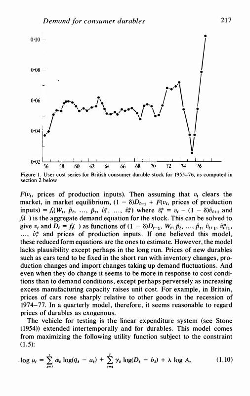
Demand for consumer durables

0·10 I 0·08

. .1···-·'·\ ;·

,,... / '. I 'e •·• ' ··•-. ·-· ·-···' � •

/ ....... , I \ I .\ ,. /�

•·•' .. .'. ...

0·04 /

v •

2 1 7

Figure I . User cost series for British consumer durable stock for 1955-76. as computed in section 2 below

F(vt, prices of production inputs). Then assuming that Vt clears the market, in market equilibrium, ( I - 8)Dt-i + F(vt, prices of production inputs) = ft( Wt. Pt • . . . , Pn vt ' . . . , vn where vt = Vt - ( I - 8)Vt+l and ft( ) is the aggregate demand equation for the stock. This can be solved to give Vt and D1 = .ft( ) as functions of ( 1 - 8)D1-i . W1, Pe . . . . , Pn vt+1 , vt+i . . . . , v; and prices of production inputs . If one believed this model, these reduced form equations are the ones to estimate. However, the model lacks plausibility except perhaps in the long run. Prices of new durables such as cars tend to be fixed in the short run with inventory changes , pro­duction changes and import changes taking up demand fluctuations . And even when they do change it seems to be more in response to cost condi­tions than to demand conditions, except perhaps perversely as increasing excess manufacturing capacity raises unit cost. For example, in Britain , prices of cars rose sharply relative to other goods in the recession of 1974-77. In a quarterly model , therefore, it seems reasonable to regard prices of durables as exogenous.

The vehicle for testing is the linear expenditure system (see Stone ( 1954)) extended intertemporally and for durables. This model comes from maximizing the following utility function subject to the constraint ( 1 .5):

T T · log Ut = L as log(qs - as) + L l's log(Ds - bs) + >.. log Ar

s� s=t ( 1 . 10)

2 1 8 J . M U E L L B A U E R

where '2: a8 + '2: Ys + A = l The period t demand functions are

qt = at + at (wt - ± asfis - ± hsvt) Pt t t

( 1 . 1 1)

( 1 . 12)

where Wi is defined from ( 1 .4) and ( 1 .5) . Note that, unlike previous work with the extended linear expenditure system, a8 and bs are not eliminated for all s greater than t - which would remove all price expectations - nor is W1 replaced by the plainly unsatisfactory proxy of measured income or even conventionally defined permanent income. '2:/+i a8p8, '2:[+1 b8v;' and the expected labour income component of W1 are represented by expecta­tional proxies while assets are treated explicitly.

These proxies are one way in which lags come into the model. Another way is from lagged social interactions somewhat along the lines of Due­senberry ( 1949) . Suppose the committed purchases a1 and b1 of each household are linear functions of the observed purchases in the previous period of non-durables and durables by the reference group with which the household identifies and of which it is a member. If different house­holds have the same parameters then, as Gaertner ( 1974) points out, in the aggregate the a1s and b1s are linear functions of aggregate purchases in the previous period. This motivation for lags avoids the charge of myopia which would be justified if similar lags were derived in an intertemporal context from the individualistic theory of habit formation - see, for ex­ample, Pollak ( 1970; 1978) and Phlips ( 1974).

As far as the aggregation properties of ( 1 . 1 1) and ( 1 . 12) are concerned, the as and bs can differ over households2 but for exact linear aggregation the as and {3s must be the same across households. While this may not be too bothersome for households of the same demographic structure, it is implausible for households whose heads differ widely in age . To obtain exact aggregation then it must be assumed that the distribution of W1 over age is constant over time though slightly weaker conditions permit sto­chastic aggregation - see Theil ( 1954) .

This concludes the discussion of the basic theory of the model . The more empirical questions of how to deal with seasonality , expectations , and the construction and use of the asset and stock data on durables are discussed in the next section.

The essence of the proposed test is as follows. The extended linear expenditure system ( 1 . 1 1) and ( 1 . 12) is applied to quarterly British data on non-durable purchases and stocks of durables . One implication of ( 1 . 1 1 ) and ( 1 . 12) lies in the restrictions across equations on various parameters

Demand for consumer durables 2 1 9

and these are tested. Independently of any specific functional form restrictions , ( 1 .8) implies that all the elements which make up long-run purchasing power are wrapped up in the variable Wt. These include ex­isting financial and real assets, current income and discounted expected labour income. Because the same Wt appears in both equations , the parameters which reflect the proxying of income expectations ought to be the same in both equations and this gives a more robust test in which the other cross-equation parameter restrictions of ( 1 . 1 1 ) and ( 1 . 12) are ig­nored.

2 Empirical implementation of the extended linear expenditure system

Seasonality

In practice, it is necessary to take seasonal differences in expend­iture into account. This is done by permitting at and Yt to differ between quarters. This allows seasonal effects to expand with expenditure rather than to remain either absolutely fixed or to expand with lagged q and D, which would be the result of the more obvious procedure of allowing sea­sonal variation in the committed quantities a and b. Attaching seasonal ef­fects to lagged values of q and D would raise the problem of whether to interpret large positive coefficients on lagged variables of q and D as re­flecting genuine lags or merely widening seasonal effects .

Expectations

Two alternative formulations of the expectational proxies were tried and they will be illustrated by taking the case of labour income . The first assumes that income expectations are generated in money terms. We want to proxy

± Ys = Yt ( 1 + ± YslYi) t t+l

Now suppose Ys+i!Ys = 1 + Pt, s = t + 1 , . . . , T. Then T

L Ys/Yt = 1 + ( 1 + Pt) + ( 1 + Pt)2 + . . . + ( 1 + Pty-1 t

(2. 1)

= [( 1 + PtY - 1]/ Pt (2.2)

By the first three terms of the Binomial expansion this is a linear function of Pt· Now we suppose that expectations on p1 are given as the weighted average of some steady state view p0 and recent experience. The latter is

220 J . M U E L L B A U E R

represented by (IA)DFD(y,) where DFD(y,) is the 'discounted fourth dif­ference of income' which is [ytf 0 + r,)( 1 + 't-1)0 + rt-2)0 + rt-a) - Yt-4]/Yt-4• Note that the first term in [ ] is exactly the discounted in­come which would have been relevant one year ago had incomes been correctly anticipated. Working with annual changes removes seasonal ir­regularities and, as Davidson, Hendry et al. ( 1978) argue, is likely to re­flect the way in which consumers themselves make forecasts . Thus

L Yt = vtOinearfunction ofDFD(yt)) t (2.3)

The terms 'Li a8p8 and '2:.[ bsfjf are similarly represented by GtPt x (linear function of DFD(pt)) and btvf x (linear function of DFD(vt)) , where a, and bt are themselves respectively linear functions of expenditure on non-durables and the stock of durables one year ago. This represents the lagged spread of behaviour patterns discussed at the end of section 1 .

To meet the potential charge that the conclusions rest on the specific expectational hypothesis rather than on the neoclassical model in itself, a second expectational hypothesis was investigated. This assumes a similar structure to that above for the generation of expectations on non-durable prices but takes a much more flexible view for incomes and durable prices . The term in ( 1 . 1 1) and ( l . 1 2) which involves expectations is 'Li Ys - 'Ll asfJs - 'Li b8vf which we can write as

(2.4)

It seems reasonable to think that consumers regard the terms a8/ at and b./ ht as fairly constant and, with a similar discounting structure in y8, Ps and vf , it makes sense to proxy the terms

L Ys L (bs/ bt)vt L (a./ at)Ps

and L (as/ at)Ps

by fairly general distributed lags in real income ytf Pt and the relative price of durables vt !Pt· That expectations might be generated in real terms in this way does make sense: even with inflation running at 25% per annum one would not expect that consumers' expectations of real long-term la­bour (and transfer) income would alter by much because of inflation itself. The same thing goes for the relative price of durables, where short-term increases in capital gains because of general inflation are unlikely to lead to permanent reductions in durable rental prices, because the interest rate will eventually adjust to inflation. Further, while the expectational hy­pothesis in (2.3) may be reasonable for non-durable prices it suffers from an objection when applied to income. The transitory component in in­come changes is likely to be much more considerable than in price changes. The disadvantage of (2.3) is that current income Yt is always

Demand for consumer durables 22 1

taken as the base for projections even when it is particularly high or low because of transitory components. In fact, it turned out that the second expectational hypothesis gave better empirical results than the first though the results of the tests were similar in the two cases.

The role of financial assets

In the exposition of the neoclassical model it was assumed that the financial asset is not subject to revaluation in its money value . In re­ality , households own a wide range of financial assets, from money and other liquid assets to claims on life insurance companies and pension funds, and government and company securities. For a number of reasons it may not be relevant to measure assets A by the sum total of the market value of household net worth. In the first place, even for a single house­hold, fluctuations in the value of marketable securities may have limited relevance within the total portfolio. By the argument of Stiglitz ( 1970) , a risk averse widow living in an inflation free environment could arrange the maturity pattern of her portfolio to guarantee a constant income every period. Asset price changes would not alter her ability to do this, though of course inflation in consumer goods would make this an undesirable ob­jective and would make the total purchasing power in terms of consumer good prices of financial assets once more a good proxy for long-term pur­chasing power. A second point is that, especially in the wealthiest house­holds, part of assets will be held for bequest, and then for tax or other reasons a specific composition of assets may be desired so that again the simple money value of the aggregate is not a sufficient measure. Note, however, that the aggregate value of bequests is included in the utility function. Finally the personal sector includes not only family trusts, but also unincorporated enterprises such as small builders , retail shops , farm­ers and stockbrokers as well as non-profit institutions such as private schools, trade unions, friendly societies and universities. Hence, personal savings and asset holdings contain a substantial element not relevant to the consumption decisions of households, as usually defined. In the empirical work below, some allowance (although necessarily crude) will be made for these factors. The lower relevance of many non-liquid assets is modelled by letting A = LA + {3NLA, for liquid and non-liquid assets LA and NLA where f3 is expected to be substantially less than unity . In the British national accounts the accumulation of housing and land is treated as part of the accumulation of personal sector assets. Thus total At including housing and land is constructed from the formula

(2.5)

where St is personal saving and !l.Pt At-i . which represents asset revalua­tion, uses a specially constructed price index Pt based on price indices of

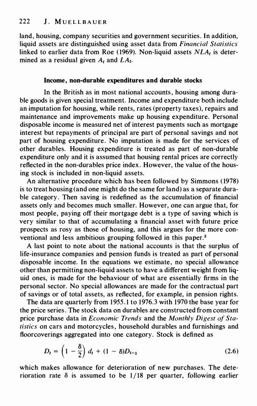
222 J . M U E L L B A U E R

land, housing, company securities and government securities . In addition, liquid assets are distinguished using asset data from Financial Statistics linked to earlier data from Roe ( 1969). Non-liquid assets NLAt is deter­mined as a residual given At and LAt.

Income, non-durable expenditures and durable stocks

In the British as in most national accounts , housing among dura­ble goods is given special treatment. Income and expenditure both include an imputation for housing, while rents, rates (property taxes), repairs and maintenance and improvements make up housing expenditure. Personal disposable income is measured net of interest payments such as mortgage interest but repayments of principal are part of personal savings and not part of housing expenditure. No imputation is made for the services of other durables. Housing expenditure is treated as part of non-durable expenditure only and it is assumed that housing rental prices are correctly reflected in the non-durables price index . However, the value of the hous­ing stock is included in non-liquid assets.

An alternative procedure which has been followed by Simmons ( 1978) is to treat housing (and one might do the same for land) as a separate dura­ble category. Then saving is redefined as the accumulation of financial assets only and becomes much smaller. However, one can argue that, for most people, paying off their mortgage debt is a type of saving which is very similar to that of accumulating a financial asset with future price prospects as rosy as those of housing, and this argues for the more con­ventional and less ambitious grouping followed in this paper.3

A last point to note about the national accounts is that the surplus of life-insurance companies and pension funds is treated as part of personal disposable income. In the equations we estimate, no special allowance other than permitting non-liquid assets to have a different weight from liq­uid ones, is made for the behaviour of what are essentially firms in the personal sector. No special allowances are made for the contractual part of savings or of total assets, as reflected, for example, in pension rights.

The data are quarterly from 1955. 1 to 1976.3 with 1970 the base year for the price series . The stock data on durables are constructed from constant price purchase data in Economic Trends and the Monthly Digest of Sta­tistics on cars and motorcycles , household durables and furnishings and floorcoverings aggregated into one category. Stock is defined as

Dt = ( 1 - &) dt + ( 1 - l>)Dt-1 (2.6)

which makes allowance for deterioration of new purchases. The dete­rioration rate 8 is assumed to be 1 / 18 per quarter, following earlier

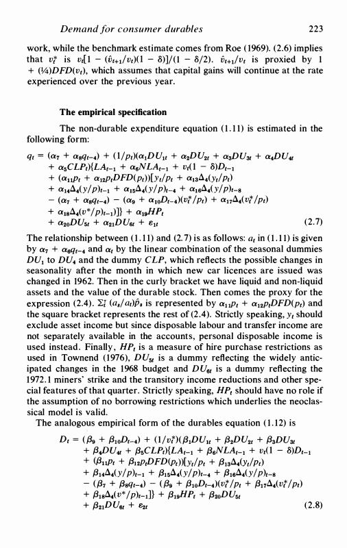
Demand for consumer durables 223

work, while the benchmark estimate comes from Roe ( 1969). (2.6) implies that vf is Vt[ l - (i!t+i!Vt)O - 8)]/(1 - 8/2) . Vt+i!vt is proxied by 1 + (IA)DFD(vt), which assumes that capital gains will continue at the rate experienced over the previous year.

The empirical specification

The non-durable expenditure equation ( 1 . 1 1) is estimated in the following form:

qt = (a1 + asqt-4) + ( lf pt)(a1DUit + a2DU2t + aaDUat + a4DU4t + a5CLPt){LAt-1 + asNLAt-1 + Vt( l - 8)Dt-1 + (auPt + a12P1DFD(pt))[Ytf Pt + alaA4(ytf pt) + a14A.iy/p)t-1 + alsA.iy/p)t-4 + alsA.iy/p)t-s - (a1 + asqt-4) - (a9 + aloDt-4)(vtf pt) + a11A.ivtfpt) + alsA.iv*/p)t-1)]} + au/fPt + a2oDUst + a21DUst + Bit (2.7)

The relationship between ( 1 . 1 1) and (2. 7) is as follows: at in ( 1 . 1 1) is given by a1 + a6qt-4 and at by the linear combination of the seasonal dummies DU1 to DU4 and the dummy CLP, which reflects the possible changes in seasonality after the month in which new car licences are issued was changed in 1962. Then in the curly bracket we have liquid and non-liquid assets and the value of the durable stock. Then comes the proxy for the expression (2.4) . 'Ll (a8/ at)Ps is represented by a1 1pt + a12p1DFD(pt) and the square bracket represents the rest of (2 .4). Strictly speaking, Yt should exclude asset income but since disposable labour and transfer income are not separately available in the accounts, personal disposable income is used instead. Finally , HP1 is a measure of hire purchase restrictions as used in Townend ( 1976), DU51 is a dummy reflecting the widely antic­ipated changes in the 1968 budget and DU6t is a dummy reflecting the 1972. 1 miners' strike and the transitory income reductions and other spe­cial features of that quarter. Strictly speaking, HP1 should have no role if the assumption of no borrowing restrictions which underlies the neoclas­sical model is valid.

The analogous empirical form of the durables equation ( 1 . 12) is

Dt = ({39 + /31oDt-4) + ( 1/vt}(f31DUit + /32DU2t + /3aDUat + /3�U4t + f3sCLPt){LAt-1 + f3sNLAt-1 + VtO - 8)Dt-1 + (/3uPt + /312PtD FD(pt) )[ytf Pt + /31aA.iytf Pt) + f314A.iy/p)t-1 + f31sA.iy/p)t-4 + f316A.iy/p)t-s - (/31 + /3sqt-4) - ({39 + /31oDt-4)(vtf pt + f311A.ivtf pt) + /31sA.iv* /p)t-1]} + f319HPt + /32oDUst + /321DU6t + B2t (2.8)

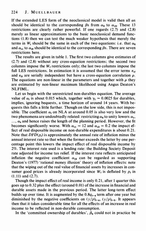
224 J . M U E L L B A U E R

If the extended LES form of the neoclassical model is valid then all as should be identical to the corresponding {3s from as to a18• These 13 restrictions are clearly rather powerful. If one regards (2.7) and (2.8) merely as linear approximations to the basic neoclassical demand func­tions ( 1 .8) then we can test the much weaker hypothesis that merely the terms in Wt should be the same in each of the two equations : i .e . that as and au to a16 should be identical to the corresponding {3s . There are seven restrictions here.

The results are given in table 1 . The first two columns give estimates of (2. 7) and (2.8) without any cross-equation restrictions ; the second two columns impose the Wt restrictions only; the last two columns impose the full LES restrictions. In estimation it is assumed that the error terms 811 and 82t are serially independent but have a cross-equation correlation p. The equations are non-linear in the parameters and together with p they are estimated by non-linear maximum likelihood using Angus Deaton's NLFIML.

Let us begin with the unrestricted non-durables equation. The average value of at is about 0.015 which, together with Yt = 0.0025 for durables, implies, ignoring bequests , a time horizon of around 14 years . With be­quests this falls a little further. Though on the low side, this is not impos­sible. The coefficient at on NLA at around 0.05 is also very low and the two phenomena are undoubtedly related: restricting as to unity lowers ai. . . . , a4 and hence raises the length of the planning period. However, the fit becomes significantly worse. With au = 1 2 and a13 = 0.2 the impact ef­fect of real disposable income on non-durable expenditures is about 0.21 . Note that DFD(pt) i s approximately the annual rate of inflation minus the annual interest rate so that when the former exceeds the latter by one per­centage point this lowers the impact effect of real disposable income by 2%. The interest rate used is a lending rate : the Building Society Deposit rate adjusted for income tax relief. If the interest rate reflects anticipated inflation the negative coefficient a12 can be regarded as supporting Deaton's ( 1977) ' rational money illusion' theory of inflation effects: note that the wiping out of the real value of financial assets by increases in con­sumer good prices is already incorporated since Wt is deflated by Pt in (1 . 1 1) and (2.7).

Though the impact effect of real income is only 0.2 1 , after 1 quarter this goes up to 0.32 plus the effect (around 0.01) of the increase in financial and durable assets made in the previous period. The latter long-term effect builds up over time. It is augmented by the 0.8qt_4 term after one year but diminished by the negative coefficients on (y/p)t-4, (y/p)t-s· It appears then that it takes considerable time for all the effects of an increase in real income to be reflected in non-durable consumption.

In the 'committed ownership of durables ' , {39 could not in practice be

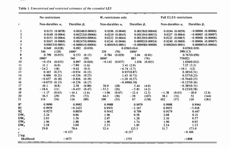
Table I. Unrestricted and restricted estimates of the extended LES

No restrictions W1 restrictions only Full ELES restrictions

Non-durables a , Durables {3, Non-durables a, Durables {3, Non-durables a, Durables {3, 1 0.0 13 1 (0.0058) 0.00248(0.00063) 0.0196 (0.0040) 0.00158(0.00049) 0.0194 (0.0059) -0.00006 (0.00006) 2 0.0148 (0.0064) 0.00252(0.00066) 0.0219 (0.0043) 0.001 19(0.00033) 0.0217 (0.0064) -0.00005 (0.00007) 3 0.015 1 (0.0064) 0.00249(0.00064) 0.0222 (0.0044) 0.00120(0.00033) 0.0221 (0.0065) -0.00006 (0.00006) 4 0.0165 (0.0069) 0.00247(0.00066) 0.0241 (0.0046) 0.00092(0.00024) 0.0240 (0.0069) -0.00006 (0.00007) 5 0.00015(0.0001) -0.00001 (0.00004) 0.00019(0.0001) -0.00009(0.00008) 0.00020(0.0001 ) 0.000003(0.00004) 6 0.049 (0.028) 0.092 (0.030) 0.050(0.014) 0.039(0.019) 7 546 ( 120) 1000* 529 (70) 1000* 590( 1 1 3) 8 0.799 (0.053) 0.533 (0. 15) 0.784 (0.029) 3.04 (0.81) 0. 767(0.050) 9 1000* 540 (59) 1000* 883 (76) 759(82)

IO -0. 154 (0.033) 0.897 (0.026) -0. 142 (0.037) 1 .036 (0.015) 1 .020(0.012) I I I I . I (6.0) -7.80 ( 1 .6) 3 .41 (2.0) 7 .25 (3.2) 12 -24.2 ( 18) -9.62 (9.5) -6.74 (3.7) - 19. 1 ( 12) 1 3 0. 165 (0.27) -0.934 (0. 13) 0.937(0.87) 0. 185(0.3 1 ) 14 0.606 (0.21) -0.556 (0.25) 1 .43 (0.71) 0.557(0.23) 15 -0.657 (0. 18) -0.826 (0. 19) - 1 .20 (0.57) -0.764(0.23) 16 -0.0753 (0. 15) -0.236 (0. 17) -0.499(0.30) -0. 127(0. 16) 17 10. 1 (8.8) 2.58 (0.80) 30.9 (28) 5.44 (4.0) -0.385(0.51 ) 18 - 1 8.6 ( 1 1 ) -0.453 (0.47) -33.2 (26) -5.81 (4.2) 0.223(0.58) 19 - 1 . 17 (0.63) - 14 . 1 ( 1 .6) - 1 .06 (0.67) - 12.4 (2.3) - 1 .38 (0.63) - 18.0 (2.6) 20 36.5 (29) 176 (72) 66.3 (30) -39 ( 107) 38. 1 (3 1 ) 52 ( 144) 2 1 1 14 (34) 1 16 (89) 109 (35) 67 ( 1 38) 102 (37) 1 10 ( 18 1 )

R' 0.9990 0.9992 0.9988 0.9979 0.9988 0.9961 Ri 0.9959 -0.2423 0.9951 -2. 167 0.9953 -5.018 R� 0.9275 0.8859 0.9142 0.709 0.9179 0.447 DW, 2.24 0.86 1 .96 0.58 2.08 0.21 ow. 2.03 1 .56 2.07 1 .28 2. 10 0.57 DW3 1 .96 1 .88 1 .90 1 .74 1 .90 0.95 ow. 2.28 2.00 2.33 1 . 85 2.24 1 .23

29.8 78.6 32.4 125.5 3 1 .7 173.0 p -0. 125 -0. 137 -0. 106 2 log

likelihood - 1673 - 1755 - 1 808

226 J . M U E L L B A U E R

identified separately from {310 and was set at 1000. Because of the negative value of {310 the term as a whole is close to zero at the mean value of D1_4 and negative for the latter part of the estimation period, thus implying that non-durables are gross substitutes for durables.

A tightening of hire purchase restrictions seems to reduce non-durable expenditure marginally and the dummies DU51 and DU61 have the antic­ipated effects.

The diagnostic statistics look quite favourable. Ri and R� are defined as 1 - SSEi/ SST1 and 1 - SSE4/ SST4 respectively where for example SSE1 is the sum of squares of residuals and SST1 is the sum of squared devia­tions around the mean of first differences of the dependent variable . DW1 is the conventional Durbin-Watson statistic while DW2, DW3, DW4 are analogous measures for 2 quarter etc. differences. Thus there seems to be no obvious sign of serial correlation in the residuals. 0- is the maximum likelihood estimate (MLE) of the standard error of the equation. The de­gree of freedom correction appropriate for an equation linear in the parameters would raise 0- from 29. 7 to about 34. 3 which still seems quite acceptable .4 f> measures the correlation in the residuals of the two equa­tions which here is negative.

Perhaps the most striking contrast in the unrestricted durables equation is in the income coefficients . When DFD(p1) is zero the income terms appear as

0.0025 --* - P1(- 8.8(y/p)1 + s.2a4(y/p)1 + 4.9a4(y/p)1-1 Vt

+ 7 .3aiy/p)1-4 + 2. Iaiy/p)i-s)

This seems to suggest that income changes rather than levels have the dominant effect, but must be considered in the context of {310, the coeffi­cient on D1_4, being about 0.9. Another notable feature of the equation is the very significant negative effect of hire purchase restrictions . This would seem to be direct evidence that the linear budget constraint hy­pothesis on which the neoclassical model is based is not valid.

The diagnostic statistics are much less satisfactory than those of the non-durables equation. The implication of negative Ri is that the fit of the equation when durable purchases is the dependent variable is very poor, since d1 = aD1• A standard error more than 2\12 times as great as for non-durables when durable purchases are on the average only 10% of non-durable expenditures supports this. The high R2 for levels is therefore quite meaningless. The Durbin-Watson statistics are strong evidence for positive first order serial correlation. But rather than taking a Cochrane-Orcutt transformation, this should be interpreted as evidence of a more fundamental mis-specification.

Then the cross-equation restrictions on the parameters in W1 are im-

Demand for consumer durables 227

posed. Note that the impact effect of real income on non-durable expendi­ture is 0. 19, which is almost tpe same as before, but that the fit of the dura­bles equation becomes quite terrible. Thus the information in the non­durables equation dominates these estimates and clearly imposes a quite unacceptable structure on the durables equation. The fall in the 2 log­likelihood is close to 120 for 7 restrictions which can therefore be strongly rejected.

When the further 6 restrictions that a7 to a10 and a17 and a18 are the same in the two equations are imposed, which correspond to the extended LES specification, the 2 log-likelihood falls by a further 53 so that the full LES specification can be strongly rejected in the framework of the unre­stricted forms of (2.7) and (2.8). Very similar results but worse fits throughout were obtained when expectations proxies of the first type con­sidered above were used.

In one respect even the unrestricted forms of (2. 7) and (2.8) are not very general: they permit only a wealth role for prices of other assets, espe­cially those of houses . Had houses been distinguished as a second type of durable in a three group system of equations , house prices could have been given a separate systematic role. Though imputed rental income from housing should then be excluded from income, the wealth term oth­erwise stays the same. As an approximation to this specification, the house price index and, for good measure, the Financial Times ordinary share index were included as extra linear terms in each equation and the tests described above repeated. Briefly, the same rejections take place: when the restrictions on the coefficients in Wt are imposed, the drop in the 2 log-likelihood is 52 for 7 restrictions which is still very significant. But it is worth noting that the fit of the durables equation is improved, though the Durbin-Watson statistics are little altered: higher house prices raise purchases of durables.

Some other checks can be carried out which are even less dependent on the specific expectational hypothesis. For example, note that from ( l . 1 1 ) and ( 1 . 12) , Pt(qt - at)!at = vt(Dt - bt)i'Yt = Wt - L a,p, - L b,v: . This implies

(2.9)

Using the empirical forms (2.7) and (2.8) the equation (2.9) becomes

Dt = {39 + /31oDt-4

+ ( {3f DUtt + {3{DU2t + {3lDUat + {3t_DU4t + {3t CLPt ) .J!L DUtt + a{DU2t + atDU3t + atDU4t + atCLPt vt

{qt - a1 - asqt-4 - <X19HPt - a2oDU5t - a21DU6t - Bit} + /31eHPt + /32oDU5t + /321DU6t + e2t (2. 10)

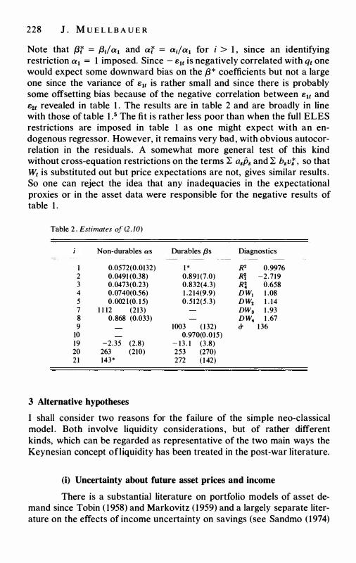
228 J . M U E L L B A U E R

Note that f3f = f3tf a1 and af = a;/a1 for i > 1 , since an identifying restriction a1 = 1 imposed. Since - e11 is negatively correlated with qt one would expect some downward bias on the /3* coefficients but not a large one since the variance of e11 is rather small and since there is probably some offsetting bias because of the negative correlation between e1t and e2t revealed in table 1 . The results are in table 2 and are broadly in line with those of table 1 . 5 The fit is rather less poor than when the full ELES restrictions are imposed in table 1 as one might expect with an en­dogenous regressor. However, it remains very bad, with obvious autocor­relation in the residuals. A somewhat more general test of this kind without cross-equation restrictions on the terms L a8p8 and L bsvt , so that Wt is substituted out but price expectations are not, gives similar results . So one can reject the idea that any inadequacies in the expectational proxies or in the asset data were responsible for the negative results of table 1 .

Table 2 . Estimates of (2. 10)

Non-durables as Durables {3s Diagnostics

I 0.0572(0.0132) I * R2 0.9976 2 0.0491 (0.38) 0.891 (7.0) Rj -2.719 3 0.0473(0.23) 0.832(4.3) R� 0.658 4 0.0740(0.56) 1 .2 14(9.9) DW, 1 .08 5 0.0021(0. 1 5) 0.512(5.3) DW2 1 . 14 7 1 1 12 (213) DW3 1 .93 8 0.868 (0.033) DW4 1 .67 9 1003 ( 132) u 1 36

10 0.970(0.015) 19 -2.35 (2.8) - 13 . 1 (3.8) 20 263 (210) 253 (270) 21 143* 272 ( 1 42)

3 Alternative hypotheses

I shall consider two reasons for the failure of the simple neo-classical model . Both involve liquidity considerations, but of rather different kinds, which can be regarded as representative of the two main ways the Keynesian concept ofliquidity has been treated in the post-war literature.

(i) Uncertainty about future asset prices and income

There is a substantial literature on portfolio models of asset de­mand since Tobin ( 1958) and Markovitz ( 1959) and a largely separate liter­ature on the effects of income uncertainty on savings (see Sandmo ( 1974)

Demand for consumer durables 229

and Deaton and Muellbauer (1980, ch. 14) . One consideration that comes out of an attempt to integrate the two approaches by setting up an appro­priate dynamic programming problem with uncertainty suggests that one might expect different income dynamics for durables than for non­durables. Suppose that for next period, income and the prices of bonds and of durables are uncertain but the price of non-durables is not. This in­troduces an asymmetry which makes the form of the solution for durables demand rather different from that of non-durables and is a possible ratio­nalization of the above results . Even if there were uncertainty about both prices one would expect, because of the capital gains element in the de­mand for durables, that uncertainty about prices of durables would be more important. However, setting up and estimating formal models of this type is a substantial research project in its own right, though it seems to me to be a feasible one.

(ii) Transactions costs

The neoclassical model predicts pronounced volatility of durable purchases. Uncertainty about the price of durables next period is one reason why one might expect only limited volatility. Another reason comes out of informational assymetries and other, more mundane trans­actions costs . A major reason for volatility lies in the assumption that, next period, durables purchased this period can be liquidated at the price prevailing next period taking into account the efficiency loss through dete­rioration at the rate 8. But as Akerlof ( 1970) points out, the potential buyer has less information on a used durable than the owner and is likely to fear that the owner wishes to sell because it is a ' lemon' . Even if it is not, there may be no cheap way the owner can give this information to the buyer. The effect is like having to pay a fixed transaction cost in order to sell. This must reduce speculative activity in durables purchases .

One way of representing this in the budget constraint is to add to the expenditure v.(D8 - ( 1 - 8)D8_1) the following non-convex transaction cost

{k1V8Ds + k2vs( 1 - 8)Ds-1 �f Ds - ( 1 - 8)Ds-1 : 0 (3 . 1 )

0 tf Ds - ( 1 - 8)D8-1 - 0

The idea is the following: let v8 be some average index of new and used durable prices . If no investment is made then D8 - ( 1 - 8)Ds-1 is zero and no transactions are carried out. Otherwise the used durable, e .g. a car, is traded in at a return of v.( 1 - k2)( 1 - 8)D8_1 where k2, which might for example be 20%, represents the transaction cost margin of selling. The new durable is bought for vs( 1 + k1)D8 where k1 is the transaction cost margin of buying. In empirical applications k1 = k2 seems a reasonable

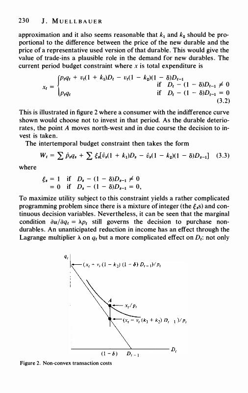
230 J . M U E L L B A U E R

approximation and it also seems reasonable that k1 and k2 should be pro­portional to the difference between the price of the new durable and the price of a representative used version of that durable . This would give the value of trade-ins a plausible role in the demand for new durables . The current period budget constraint where x is total expenditure is

Xt = if Dt - ( 1 - f>)Dc-1 f 0 {Ptqt + Vt( l + ki)Dt - Vc( l - k2)( 1 - f>)Dt-1

Ptqt if Dt - ( 1 - f>)Di-1 = 0 (3 .2)

This is illustrated in figure 2 where a consumer with the indifference curve shown would choose not to invest in that period. As the durable deterio­rates, the point A moves north-west and in due course the decision to in­vest is taken.

The intertemporal budget constraint then takes the form

where

Wt = L p.q. + L av.( 1 + ki)Ds - v.( 1 - k2)( 1 - f>)Ds-1] (3 .3)

g. = 1 if D, - ( 1 - f>)Ds-1 f 0 = 0 if D. - ( 1 - f>)Ds-1 = 0,

To maximize utility subject to this constraint yields a rather complicated programming problem since there is a mixture of integer (the g.s) and con­tinuous decision variables . Nevertheless, it can be seen that the marginal condition iJu/iJqt = A.pt still governs the decision to purchase non­durables . An unanticipated reduction in income has an effect through the Lagrange multiplier A. on qt but a more complicated effect on Dt: not only

q,

�----�--�---- D,

( 1 - '5 ) D, _ 1

Figure 2. Non-convex transaction costs

Demand for consumer durables 23 1

is there a reduction for those who had planned to invest but there is a shift in the extensive margin in the population of those making some invest­ment: some will postpone. How the latter effect operates depends on the joint distributions of income, income expectations and durable stocks and is quite different from the way these variables enter the non-durable de­mand functions. This rationalizes the quite different income dynamics found empirically in the two equations.

The demand functions conditional on the gs which come out of (3 .3) are manageable at least for certain classes of utility functions. Note that the model sketched here is most applicable to data disaggregated into specific kinds of different durables so that the budget constraint (3.3) is really de­fined for a vector of stocks of different durables . For such data aggregated across households, the mean value of gt is simply the proportion of house­holds with non-zero purchases of that durable good. The inequalities which determine gt are very complicated and involve distributional data. Thus the model is most suitable to be applied to data, especially panel data, on the purchases by individual households of particular durable goods.

When different durable goods are aggregated into one the zero-one as­pect of purchases is likely to be lost so that even on quarterly data a single household always has positive durable purchases . Aggregation over dif­ferent kinds of durables tends to smooth and make convex the non­convex adjustment costs for each kind in (3.3) . It may therefore be that, as an approximation, the assumption of convex (e.g. quadratic) adjust­ment costs at the level of aggregated durables data is a reasonable one. If so, the route leads back to the stock adjustment model but suggests two modifications to the conventional analysis. The first is that the measure of durable prices Vt should be an average of new and used prices and that ad­justment costs increase with the margin between the two. The second is that expectations should be treated more systematically than is usually the case in estimates of stock adjustment models.

Summary and conclusions

Section 1 reviews the neoclassical theory of demand for durables . The definition of 'neoclassical' here is a narrow one: optimizing consumers face given prices and endowments at which they can buy or sell, have point expectations about future prices and endowments and do not incur costs of adjustment. If, as seems plausible , costs of adjustment as usually understood are merely a proxy for non-linearities in the budget constraint, their absence is simply an implication of the assumption of given prices . Notice that point expectations excludes portfolio considerations, which is consistent with the simplifying assumption usually made in life cycle con­sumption or savings theories that financial assets can be aggregated into a

232 J . M U E L L B A U E R

single asset with a given rate of interest and not subject to revaluation. Assuming, in addition, that durables of different vintages can be ag­gregated in efficiency corrected units gives a linear intertemporal budget constraint in which the prices are the discounted prices of non-durables and the discounted user cost or rental equivalent prices of durables. The wealth term consists of the present value of current and expected income, and initial endowments of durables and the financial asset. The linear expenditure system extended intertemporally and for durables gives the demand functions for purchases of non-durables and the stock of durables a linear structure which allows the aggregate behaviourial equations to have the same form as the ones for individual households . The committed consumption levels in the ELES are assumed through the influence of lagged social interactions to depend on past consumption levels.

Section 2 begins with the treatment of expectations : it is assumed that expectations of non-durable prices, real incomes and relative prices are each formed on the basis of past observations of the dependent variable . By giving income and income expectations a quite distinct role from assets, by introducing future committed consumption levels, which makes price expectations important, and by permitting the committed consumption levels to depend upon past consumption, the form of the ELES which emerges is much more general than that of Lluch ( 1973) and Lluch, Powell and Williams ( 1977). There is also a brief review of the na­tional accounts treatment of income, savings, assets and durables to put the empirical application which follows in context. This is to quarterly data going back to 1955: the existence of the asset and durables data going back this far owes much to the work of the Stone group in Cambridge. The theory implies some cross-equation restrictions between the non­durables and durables equations and testing these is the main point of this exercise. These restrictions are conclusively rejected. One might argue that this is understandable for a particular form of utility function which may be a poor approximation to preferences . However, in much more general forms of the test, in which the ELES restrictions are ignored and only the hypothesis that the wealth term has the same asset and income expectations parameters in both the non-durables and the durables equa­tions is tested, the result is the same: rejection. This implies that non­durable purchases and durable ownership are not consistent with the same neoclassical budget constraint . Other aspects of the results worth mentioning are that the non-durables equation is quite reasonable, fits well and has residuals which look like white noise. However, non-liquid assets have a much lower coefficient relative to liquid assets than simple theory would suggest. The durables equation is rather poor with positively auto-correlated residuals even in the most general specification and very significant coefficients on the terms for credit restrictions - which is an-

Demand for consumer durables 233

other reason for arguing that behaviour i s inconsistent with the inter­temporal neo-classical budget constraint.

Section 3 suggests two possible explanations. One feature of the neo­classical model is that the rental price of durables is fairly volatile and this is one reason why the model suggests that purchases should also be vola­tile. Both of the alternative hypotheses suggest limitations on the speed of adjustment; uncertainty and transactions costs which stem from the a­symmetry of information between buyers and owners of used durables. It is suggested therefore that either or both the perfect markets (linear budget constraint) assumption and the assumption that the constraint is perceived with confidence are erroneous even as approximations. By con­sidering a model where the budget constraint is non-linear because of transactions costs, it is possible to give a theoretical justification to the empirical result that assets, income and income expectations enter the non-durables and durables equations in quite different ways.

Notes

1 Support for this research under SSRC grant HR4577 / 1 is gratefully acknowl­edged. I am indebted to Angus Deaton and Gerald Kennally for stimulating dis­cussions and comments and to Gerald Kennally for effective programming. John Dorrington and Alan Roe were helpful in providing missing pieces of data. Responsibility for errors remains with the author.

2 If households have the same price expectations. 3 However, see the discussion of portfolio models in section 3 . 4 I n the base year, 1970, quarterly non-durable consumption = 7500. 5 Not surprisingly only fn of the seasonal parameters is well determined. For

similar reasons separate estimates of a21 and {321 could not be obtained and a21 was therefore restricted.

References

Akerlof, G. ( 1970), 'The market for lemons' , Quarterly Journal of Economics, 84, pp. 488-500.

Chow, G. ( 1957), Demand for Automobiles in the US: a study in consumer dura­bles, Amsterdam: North Holland .

Cramer, J. S. ( 1957), 'A dynamic approach to the theory of consumer demand' , Review of Economic Studies, 24, pp. 73-86.

Davidson, J. E. H . , Hendry , D. F. et al. ( 1978), ' Econometric modelling of the ag­gregate time-series relationship between consumers' expenditure and income in the United Kingdom' , Economic Journal, 88, pp. 661 -92.

Deaton, A. S. ( 1977), ' Involuntary saving through unanticipated inflation' , Ameri­can Economic Review, 67, pp. 899-910.

Deaton, A. S. and Muellbauer, J. ( 1980) , Economics and Consumer Behavior, New York and Cambridge : Cambridge University Press.

Diewert, W. E. ( 1974), ' Intertemporal consumer theory and the demand for dura­bles' , Econometrica , 42, pp. 497-5 16.

234 J . M U E L L B A U E R

Duesenberry , J. S . ( 1949), Income, Saving, and the Theory of Consumer Beha­viour, Cambridge , Mass. : Harvard University Press.

Farrell, M. J. ( 1954), 'The demand for motor cars in the United States ' , Journal of the Royal Statistical Society, Series A, 117, pp. 171 -20 1 .

Fisher, I . ( 1930), The Theory of Interest , New Haven, Connecticut: Yale Univer­sity Press, 1930.

Gaertner, W. ( 1974) , 'A dynamic model of interdependent consumer behaviour' , Zeitschrift fur Nationa/Okonomie, 34, pp . 327-44.

Haavelmo, T. ( 1960), A Study in the Theory of Investment, Chicago : University of Chicago Press.

Hess, A . C. ( 1977), 'A comparison of automobile demand equations ' , Econome­trica, 45, pp. 683-702.

Jorgenson, D. W. ( 1963), 'Capital theory and investment behaviour' , American Economic Review, 53, Papers and Proceedings, pp. 247-59.

Lluch, C . , ( 1973), 'The extended linear expenditure system' , European Economic Review, 4, pp . 2 1 -32.

Lluch, C., Powell, A. A., and Williams, R. A . ( 1977), Patterns in Household De­mand and Saving, Oxford University Press.

Markowitz, H. M. (1959), Portfolio Selection, John Wiley. Modigliani, F. and Bromberg, R. (1955), 'Utility analysis and the consumption

function : an interpretation of cross-section data' , in Kurihara, K. K. (ed.) , Post Keynesian Economics , George Allen & Unwin, London.

Phlips, L. ( 1974) , Applied Consumption Analysis , North-Holland , Amsterdam and Oxford.

Pollak, R. A. ( 1970), ' Habit formation and dynamic demand functions' , Journal of Political Economy, 78, pp. 60-78.

( 1978) , 'Endogenous tastes in demand and welfare analysis' , American Eco­nomic review, 68, (papers and proceedings), pp . 374-9.

Ramsey, F. P. ( 1928), 'A mathematical theory of saving' , Economic Journal, 38, pp. 543-59.

Roe, A. ( 1969), •A quarterly series of personal sector assets and liabilities' , Cam­bridge Growth Project Paper no. 8, mimeo.

Sandmo, A. ( 1974), 'Two-period models of consumption decisions under uncer­tainty: a survey' , pp. 24-35 in Dreze, J. H. (ed. ) Allocation under Uncer­tainty: Equilibrium and Optimality, Macmillan .

Simmons, P. J. ( 1978), Models for the analysis of consumer demand in the post-war UK, unpublished PhD thesis, Southampton University .

Smith, R. P. ( 1974), 'A note on car replacement' , Review of Economic Studies, 41, pp. 567-70.

( 1975) , Consumer Demand for Cars in the U.S.A . , Cambridge University Press. Stiglitz, J . E . ( 1970), 'A consumption-oriented theory of the demand for financial

assets and the term structure of interest rates' , Review of Economic Studies, 37, pp . 321 -5 1 .

Stone , J . R . N. ( 1954), 'Linear expenditure systems and demand analysis: an ap­plication to the pattern of British demand' , Economic Journal, 64, pp. 5 1 1 -27.

Stone , R. and D. A. Rowe ( 1957), 'The market demand for durable goods' , Econo­metrica, 25, pp. 423-43.

( 1958) , 'Dynamic demand functions: some econometric results' , Economic Journal, 68, pp. 256- 70.

Demand for consumer durables 235

Theil, H . ( 1954), Linear Aggregation of Economic Relations, Amsterdam: North-Holland .

Tintner, G. ( 1938), 'The theoretical derivation of dynamic demand curves' , Econ­ometrica , 6, pp. 375-80.

Tobin, J. ( 1958), ' Liquidity preference as behaviour towards risk' , Review of Eco­nomic Studies, 25, pp. 65-86.

Townend, J. C. ( 1976) , 'The personal savings ratio' , Bank of England Quarterly Bulletin , 16, pp. 53-73.

Westin, R. B. ( 1 975), 'Empirical implications of infrequent purchase behaviour in a stock-adjustment model' , American Economic Review, 65, pp. 384-96.

9 Liquidity and inflation effects on consumers' expenditure1

DAV I D F . H E N D R Y

A N D T H O M AS V O N U N G E R N - S T E R N B E R G

1 Introduction

In a recent study of the time-series behaviour of consumers' expenditure in the United Kingdom, Davidson et al. ( 1978) (denoted DHSY below), presented results for an equation in constant (1970) prices, relating con­sumers' expenditure on non-durables and services (C) to personal dispos­able income ( Y) and the rate of change of prices (P):

A4c1 = aiA4Yt + a2A1A4Yt + aaA4Pt + a4A1A4Pt + a:;(Ct-4 - Yt-4) + asAJ>t + Bt (1)

In (1) , lower case letters denote loge of corresponding capital letters , P1 is the implicit deflator of C1, AJ = ( 1 - IfJ) where .:£kxi = Xt-k and Bt is as­sumed to be a white-noise error process. D1 is a dummy variable for 1968(i) and (ii) and for the introduction of VAT.

DHSY selected equation (1) using the criteria that it: (i) encompassed as special cases most previous empirical models re­

lating C1 to Yi; (ii) was consonant with many steady-state economic theories of non­

durable consumption; (iii) explained the salient features of the available data; (iv) provided a simple dynamic model in terms of plausible decision vari­

ables of economic agents; (v) helped explain why previous investigators had selected their (pre­

sumed incorrect) models; (vi) exhibited an impressive degree of parameter constancy over twenty

quarters after the end of the estimation sample (through a period of rapid change in P and C/ Y).

Nevertheless, DHSY did not conclude that ( 1) represented a ' true' struc­tural relationship and three issues merited immediate re-examination, namely, liquidity effects , the role of inflation, and the treatment of season­ality .

Although DHSY obtained negative results when investigating liquid

237

238 D . F . H E N D R Y & T . VON U N G E R N - ST E R N B E RG

asset effects in ( I ) , Professor Sir Richard Stone established a significant influence for cumulated savings on consumers' expenditure using annual data (see, for example, Stone ( 1966) and ( 1973)). Moreover, the dynamic specification of (1) is logically incomplete as some latent asset stock must be altering when total expenditure is unequal to income. Alternatively ex­pressed, in the terminology of Phillips ( 1954) and ( 1957), the formulation in ( 1 ) includes derivative and proportional control mechanisms but omits integral control , and the influence of liquid assets is considered below as an observable proxy for such an integral control. This interpretation is close to the spirit of Professor Stone's approach. Integral correction mechanisms are analysed in section 2, together with a pilot Monte Carlo study of the finite sample properties of least-squares estimators in such models .

Several theories have been offered to account for the direct influence of inflation on savings (see, for example, Deaton ( 1977), Bean ( 1978) and the references therein) and in section 3 we consider the model developed in Ungem-Sternberg ( 1978) based on the mis-measurement of real income in inflationary conditions . The resulting equation avoids the problem in ( 1 ) that, as inflation increases, C/ Y falls without a positive lower bound.

The empirical evidence for the UK is re-examined in section 4 using an extension of ( 1 ) which allows for a seasonally varying average propensity to consume and thereby explains one of the 'paradoxes' noted by DHSY. Section 5 concludes and summarises the study .

Since ( 1 ) accounts for much previous empirical research relating C to Y in the UK, we commence from DHSY's model and supplant it by an equa­tion which still satisfies the six criteria noted above. Although the re­sulting model remains parsimonious, is data coherent and exhibits a fair degree of parameter constancy, it is undoubtedly far from being the final resolution of this complex subject. It is offered as a further step in that sci­entific progression which has been a hallmark of Professor Stone's re­search.

2 Integral correction mechanisms

Simple dynamic models based on 'error correction' feedbacks as in ( 1 ) are important in linking equations formulated in levels with those formulated in differences of the original variables. Further, an error correction model (denoted ECM) has many interesting dynamic and econometric properties (see, for example, Sargan ( 1964), DHSY and Hendry ( 1980)) and, appro­priately specified, can ensure that an estimated equation reproduces as its steady-state solution the economic theory from which it was derived, thus facilitating rigorous testing of theories. Consequently, ( 1 ) provides an ex­ample of a useful class of dynamic equations.

Liquidity, inflation and consumption 239

Nevertheless , (1) has a major flaw as a complete account of the dynamic behaviour of flow variables . Consider the simplest example of an ECM relating two variables denoted by wi and xi:

(2)

where Vt - NI(O, er�) and E(xiv.) = 0 V t, s, with 1 > y1 , y2 > 0. The non­stochastic steady-state solution of (2) when d1xi = g must have d1Wt = g and hence:

W = KX where K = exp((y1 - l)g/y2) (3)

and (2) is stable provided 2 > y2 > 0. However, the convergence of Wt to its steady-state growth path following any disturbance is monotonic and if y1 < 1 then wi converges to xi + k from below (above) when xi increases (decreases) (note that, in terms of stabilising W /X, d1xt has the appropri­ate negative coefficient). Consequently, even when K = 1 (k = 0) there is a cumulative underadjustment if xi is steadily increasing or decreasing. If Wt is an expenditure and xi an accrual then some stock of assets is impli­citly altering and for decreases in Xt is essential to finance the 'over­spending' .

In the terminology of Phillips ( 1954 and 1957), (2) incorporates deriva­tive (d1xt) and proportional (xi-1 - Wi-1) control mechanisms, but no inte­gral control (L;<t (x; - w;)) . Such an integral can be interpreted most easily by introducing a state variable A1 (which may or may not be observ­able) defined by (using end-of-period definitions):

(4)

In terms of the original variables, A1 is the integral of past discrepancies between X and W. Whether or not integral control mechanisms (denoted by ICMs) influence behaviour is, from this viewpoint, simply a matter of dynamic specification. Nevertheless, economic theory is far from being devoid of alternative interpretations (for example, Pissarides (1978) presents a theoretical analysis of the role of liquid assets in consumption which yields conclusions similar to those obtained below) and we record with interest that Phillips (1954, p. 3 10) considered the 'Pigou Effect' to be an integral regulating mechanism inherent in the economy.

Indeed, many previous researchers have incorporated integral vari­ables in expenditure equations, including the explicit use of cumulated savings by Stone ( 1966) and ( 1973), liquid assets (see, inter alia, Zellner et al. (1965) and Townend ( 1976)) and wealth (see Ball and Drake ( 1964), Deaton (1972; 1976) and Modigliani ( 1975)). However, since there are many econometric relationships in which integral effects are potentially relevant but do not appear to have been used previously (such as wage-price equations) we develop the simplest form of model which ex-

240 D . F . H E N D R Y & T . V O N U N G E R N - S T E R N B E RG

tends (2) to allow for an ICM, following an approach similar to Deaton (1972) and Hendry and Anderson (1977).

To focus attention on the dynamic specification, we assume that a prior steady-state utility maximization exercise leads agents to seek to maintain constant ratios both between W and X as in (2) and between A and X (ce­teris paribus) , namely: we = K*X and Ae = B*X where e denotes 'dynamic equilibrium' . For consistency with (4) in steady state, K* = 1 - (g/( 1 + g))B* . Either linear or log-linear decision rules could be for­mulated, but since we want the latter in order to generalize (2) (noting also that both DHSY and Salmon ( 1979) found Sargan's ( 1964) likelihood crite­rion favoured log-linear models for Ct) , (4) has to be replaced by its steady-state approximation:

.11 af = H*(xt - w1) where H* = (1 + g)/B*

The long-run targets can be written in logs as :

wf = k* + x1 and af = b* + Xt

(5)

(6)

Since the actual outcomes are stochastic , and (4) rather than (5) holds for the observed data, disequilibria can occur. To model agents assigning priorities to removing these, a quadratic loss function is postulated where the first two terms are the relative costs attached to discrepancies occur­ring between planned values (wf and af) and their respective steady-state outcomes. Further, to stabilize behaviour when the environment remains constant (i .e . to avoid 'bang-bang' control in response to random fluctua­tions), agents attach costs to changing wf from Wt-l · However, when the primary objectives are to attain (6) , it does not seem sensible to quadrati­cally penalize changes in wf when it is known that w{ has changed. Thus there is an offset term to allow more adjustment at a given cost when wf has changed than when it is constant. By comparison, partial adjustment models enforce quadratic adjustment costs irrespective of how much the target is known to have changed.

Collecting together these four terms in a one-period loss function yields:

qt = A1(af - Xt - b*)2 + A2(wf - Xt - k*)2 + Aa( wf - Wt-1)2 - 2A4( wf - Wt-1)(Xt - Xt-1) (7)

where A; 2::: 0 (i = 1 , . . . , 4) . Allowing for the possibility that the current value of x1 might be uncertain, E(q1) has to be minimized with respect to wf (or af), taking account of (5) holding for planned quantities. The delib­erately myopic formulation in (7) naturally leads to a ' servomechanism' solution when Xt is known, or more generally on setting (aE(qt)/awf) to zero:

Liquidity , inflation and consumption 24 1

where al.it = E(Xt) - Xt-1' Wt - wf = llt - NI(O, ai) independently ofwf and the 8; E (0, 1) are given by:

80 = (>,2k* - A.1H*b*)/tfi, 81 = (H*A.1(H* - 1) + A.2 + A.4)/tfi

82 = (H*2A.1 + A.2)/tfi, 8a = H*A.1/l/J and t}I = (H*2A.1 + A.2 + A.3)

The three variables in (8) correspond respectively to derivative, propor­tional and integral control mechanisms as required; the equivalent partial adjustment cost function would constrain 81 + 83 to equal 82 (which, in the absence of an ICM, entails having prior information that 81 = 82 , i .e . that Xt-1 does not occur in the equation).

The planning rule for w1 given by the above approach is of the form advocated by Richard ( 1980) , where agents' behaviour is described by con­ditional expectations functions, but agents have no control over the varia­bility around the function. Indeed, the uncertain and highly variable na­ture of real income makes a feedback control model like (8) an attractive behavioural possibility for expenditure. Also, the inclusion of specific mechanisms for correcting past mistakes makes the white-noise assump­tion for u1 more tenable .

Let Xt - Xt = Bt - N/(0, er!), then (8) holds with al.it replaced by alxt and u1 by v1 = u1 - 81e1 where E(x1v1) = - 81CT!. Conversely, time ag­gregation could introduce simultaneity between x and the equation error for the observation period even if x1 is weakly exogenous in the decision time period (see Richard, 1980) ; these two effects will be offsetting and are in principle testable, but, for the remainder of this paper, both are as­sumed to be absent.

Equation (8) seems to be the simplest generalization of (2) which incor­porates an integral control and it yields a non-stochastic steady-state solu­tion when alXt = g = alwt = alat given by:

W/X = D(A/X)"' (9)

where </> = 83/82 > 0 and D = exp{(80 - ( 1 - 81)g)/82} . Moreover, (5) (for planned magnitudes) and (8) imply that:

alat = H*{8a(X1-1 - Gi-1) - 80 + (1 - 82)(X1-1 - W1-1) + ( 1 - 81)a1x1 - um ( 10)

(where u? deviates from u1 by a term involving the product of the disequi­libria in the two endogenous variables). Consequently , in non-stochastic steady state:

A = BX or a = b + x

and hence

W = KX or w = k + x

( 1 1)

( 1 2)

242 D . F . H E N D R Y & T . V O N U N G E RN - S T E RN B E RG

where k = -gB/( 1 + g) (i.e. K = 1 - gB/(1 + g), and

(b + MB) = (b* + MB*) + (.\4 - A3)k* /.\1 ( 1 3)

when M = .\3k* /.\1(1 + g). Expanding (b + MB) in a first-order Taylor series around b* yields b = b* + (.\4 - .\3)gk* /(g.\1 .,,... A3k*2) = b* + O(g/( 1 + g)) .

Equations ( 1 1) and ( 12) reproduce the forms of the 'desired' relation­ships in (6), and show that the long-run ratios depend on the agents' aims and on the losses attached to the various terms in the objective function (7). Since only two alternatives are allowed (e .g. spending W1 or saving a1A1), W = X when g = 0, but in practice this restriction need not hold for a sub-category of expenditure.

The dynamic reaction of w1 to exogenous changes in x1 can be expressed in the form:

( 14)

and '11( . ) is the same for the autoregressive-distributed lag representation of a1 (using (5) and ( 10)), where:

'11(.:t') = { l - (1 + ( 1 - 82) - 83H*)!:t + ( 1 - 82)!£2} 2

= L l/J;!:fi ( 15) i=O ( 15) is identical to the lag polynomial of the simple multiplier-accelerator model and has stable roots since 0 < 82 , 83H* < 1 , the roots being a com­plex conjugate pair if (83H*)112 > Y2(82 + 83H*), in which case the adjust­ment path is oscillatory with period of oscillation given by 2TT/f> where cos 5 = (-l/li/2(1/12)112) (for an exposition see Allen, 1963, ch. 7) .

Changes in x1 have an impact elasticity of 81(1 - 81) on w1(a1) , and for 81 "I 1 , discrepancies are created between the actual values of A1 and W1 and their 'equilibrium' levels BX and KX respectively, both of which are partly corrected in the next period. In fact, even if 81 = 1 , the ECMs are still required to correct for stochastic variation (i.e . unless u1 = 0 V t) or for 'unanticipated' changes in x1, when that variable is not known for cer­tain till the end of the period.

Rather little is known about the finite sample properties of least-squares estimators of the 81 in (8), both when the equation is correctly specified and when the lag structure has been wrongly formulated. The case 83 = 0 was investigated by DHSY and here we consider the one set of parameter values : (80, 8., 82, 83) = ( - 0. 1 , 0 .5 , 0.3, 0. 1 ) at sample sizes T = (20, 40, 60, 80) when the model is: (i) correctly formulated; (ii) the ICM is omitted; (iii) both the ICM and the proportional ECM are omitted. <T� = 1 , <T� = 0 and x1 was generated by:

Liquidity , inflation and consumption

x, = 0 .8x1_1 + e1 with e1 - NI(O, 9)

243

The first 50 values of each data series were discarded in every replication, and each experiment was replicated 400 times, identical random numbers being used across the three sets of experiments . Normalizing on A.1 = I , the underlying parameter values are (y2 , y3 , y4) = (0.97, 2.58, I . IO) with g = 0 and h* = - I . These parameter values were selected to mimic the empirical results reported below; the chosen model has a static equilib­rium solution given by:

w = x and a = I + x

with the roots of the '11(.;t} polynomial being 0.8 ± 0.245 i. To investigate the usefulness of autocorrelation diagnostic tests as indicators of the dynamic mis-specifications, rejection frequencies for Lagrange Multiplier (LM) based tests of first and (general) fourth order residual autocorrela­tion were computed (see Godfrey, 1978; and Breusch and Pagan, 1980). The results for T = 80 are recorded in table 1 (similar outcomes were ob­tained at the other sample sizes), and several features merit note.

Firstly , the simulation findings reveal no new problems for estimating correctly specified single equations involving integral control variables since, although a1 is generated by a cumulative process as in (4), (a1 - x1) is stationary as shown in equation ( 10) . In case (i) , the coefficient biases are small and SD = SE with the residual autocorrelation tests having approximately the right empirical significance levels as found more gener­ally by Mizon and Hendry ( 1980). Dropping the ICM does not cause very large biases in iJi and 02 but does bias the intercept to zero; s2 is biased up-

Table 1 . Simulation findings for (8) at T = 80

61 9, 63 60 s2 z.( 1) z.(4)

Bias* 0.00 0.01 0.01 -0.01 0.00 0.06 0.04 (i) SD 0.04 0.05 0.02 0 . 13

SE 0.04 0.05 0.02 0. 12

Bias -0.01 -0.03 0. 10 0.29 0. 1 1 0. 1 1 (ii) SD 0.04 0.04 0.04

SE 0.04 0.05 0 . 13

Bias -0.04 0. 10 0.76 0. 16 0.06 (iii) SD 0.05 0.05

SE 0.05 0. 15

* For coefficient estimates, this denotes the simulation estimate of E(iJ; - 91), and for z.(i) (the LM test for ith order residual autocorrelation) shows the % rejection frequency of the null of no autocorrelation; SD denotes the sampling standard deviation and SE the average estimated coefficient standard error; - denotes that the parameter in question was not estimated (and hence has a bias of ( -9i)). The sampling standard error of the estimated bias is SD/20.

244 D . F . H E N D R Y & T . V O N U N G E R N - S T E R N B E RG

wards by almost 30% and the LM tests detect significant autocorrelation in the residuals only 1 1% of the time. Further, the equilibrium solution re­mains w = x so that this mis-specification would seem to be very difficult to detect. Consequently, these findings are consistent with 'true' models like (8), generating data which are apparently well explained by equations like (2) (as reported by DHSY, for example). Except for a further large in­crease in s2, the outcome is not much changed by also dropping the pro­portional ECM (note the results obtained by Wall et al. ( 1975)) .

Thus, although (at - Xt) is highly autoregressive, dropping (at-1 - Xt-1) does not cause detectable autocorrelation in the residuals. This is impor­tant given that the derivation of equations like ( 12) is often ostensibly by differencing a stock-flow relationship (see, for example, DHSY, p. 669); such interpretations are not unique because of the two formulations of 'differencing' noted by DHSY (p. 673), and (2) can be obtained from a linear equation relating w1 to x1 and at either by filtering or by imposing invalid coefficient restrictions on the integral control, with very different implications for the error process. It should be noted that Mizon and Hendry ( 1980) found the LM autocorrelation tests to have reasonable re­jection frequencies when the error was generated as an autoregressive scheme.

There are obviously a large number of steps from obtaining simple error correction models like (8) to empirical implementation, of which aggrega­tion over agents and time, and the choice of a proxy for At, are perhaps the most important in the present context. A proper treatment of aggrega­tion is beyond the scope of this paper, but (8) still provides a useful guide to equation formulation in terms of interpretable and relatively orthogonal variables.

For Ct, the stock ofreal net liquid assets of the personal sector (denoted by Lt) seems to play a role analogous to At (complicated by portfolio ad­justments in response to changes in rates of return on other assets and durable expenditure, jointly denoted by N1) :2

Lt = ( 1 - AlPt)Lt-1 + Yt - Ct - Nt

Thus, in logs:

Allt = -AiPt + H(yt - Ct) - T/t ( 16)

where H = Y / L, T/t depends on Nt (and changes in H) and the variability of T/t is assumed to be small relative to that of AtPi and (Yi - ci). The data for P1L1 are taken from the various issues of Financial Statistics (see e.g. Table 10.3 in the June 1979 issue where PtLt = total identified less bank advances). In fact, the form of equation ( 16) points directly to the issue examined in the next section.

Liquidity, inflation and consumption 245

3 Real income and inflation

The measure of personal disposable income used by DHSY is the 'con­ventional' series reported in Economic Trends and comprises wages, sala­ries, earnings of the self-employed, rents, net interest receipts , dividends and transfer payments less direct taxes, all revalued using the implicit deflator for total consumers' expenditure. Since the personal sector is a substantial net creditor (see Economic Trends, 1978, p. 291), interest re­ceipts are a non-negligible fraction of Y; moreover, as inflation increases, nominal interest rates tend to rise, thereby increasing the interest compo­nent of Y. It seems inappropriate to measure 'real income' as increasing in such a situation, since the large nominal interest receipts are offset by capital losses on all monetary assets, which are not being deducted from the income variable used (Townend ( 1976) makes a related point, but does not estimate such an effect). It is easy to understand why the national in­come accounts should wish to calculate income as the sum of readily observable components , avoiding hard to measure and rather volatile changes in the real values of a spectrum of assets. However, if Y* , the real income perceived by consumers, differs from Y, then consumption functions based on Y will manifest predictive failure when the correlation between Y and Y* alters.

Hicks ( 1939, ch. 14) discusses the many difficulties involved in defining and measuring real income when interest rates and prices (and expecta­tions about these) are changing. One improvement over Y might be ' that accrual which would leave real wealth intact' , but despite recent improve­ments in the available statistical evidence we doubt our ability to con­struct such a quarterly time-series relevant to consumers' expenditure. Indeed, to the extent that Y* differs from Y, it must do so by some easily observable magnitude.

Since most households are aware of their liquid asset position and since the personal sector's losses on liquid assets are a major component of its overall financial loss during inflationary periods, jJL (where jJ denotes the rate of inflation) seems a prime candidate for relating perceived to mea­sured income. Moreover, aggregate data on net liquid assets (which com­prise, very roughly, 20% of wealth and 40% of financial assets) seem rea­sonably accurate and will occur in our models as the basis of the ICM in any case. Thus the simplest initial hypothesis is that Y* = Y - {3jJL where {3 has been introduced to account for any scale effects due to wrongly choosing measures for jJ or L; note that if {3 = 1 (i.e. ifthe loss on our measure of net liquid assets is the variable which consumers perceive as negative income), then ( 16) could be rewritten as a1 lt = H0(yt* - Ct) - 'Y/t where H0 = Y*/L.

More or less inclusive measures proxying At could be chosen, and the

246 D . F . H E N D R Y & T . V O N U N G E R N - S T E R N B E RG

validity of these is open to test on the data. For example, the choice of L entails that agents react asymmetrically to erosion of their deposits in Building Societies as against their mortgages from the same institutions, but, to the extent that such variables behave similarly, the scaling will be corrected by {3 (for example, Building Society Mortgages are about 40% of L and are very highly correlated with L). A two-year moving average of the quarterly inflation rate of the Retail Price Index (R) was selected for p (i.e. p = A8 loge Rt/8).

To give some idea of the magnitude of the correction to real income in­volved in Y* , if f3 = 1 and p = 0.05 (per quarter) then, using L/ Y = 3 , Y* = Y(l - p(L/Y)) = 0.85 Y, inducing a dramatic reduction in the in­come measure. As p increases, L falls so that pL/ Y does not increase without bound, unlike the linear term in A4 ln P, in (1) . Further, when p is small, Y* and Y are very highly correlated and this breaks down only when inflation increases substantially ; consequently, if C = f( Y*), but models attempted to explain C by Y, then such equations would fail only whenp altered rapidly. Moreover, the increase inp in the 1970s in the UK is closely correlated with the fall in L/ Y (see figures 1 and 2) and hence in­cluding p alone as a linear regressor (as DHSY do, for example) would

0·225

J • --• L\ 4 log e R1

0·200

0•175

0·150

<>----<> L\.4 Iog e P,

0·125

0·100

0·075

f L - �

l\ ) l \ . • r1· ! /0

0-050 �- A. l�\-1.1 1�·,··· , .

0·025 WI ·� w· .. ,... v O·OOO • \.

1958(i)

Figure I

1963(i) 1968(i) 1970(iv) 1975(iv) 1977(iv)

1'15

1 ' 10

1·05

1-()()

0·95

0·90

0·85

0·80

Liquidity , inflation and consumption

• --• log e ( � ) . ,, J. ,-'\ ···�· ,··· �· . ,•

AJ)··i· . · · ·· \\ ·�J\ .

� . \ \A . \

. \ / '• . '•

247

0·75 '-----,--------,-----,--------,----,----

1963(i) 1968(i) 1971(i) 1976(i) 1977(iii)

Figure 2

provide an excellent proxy for pL/ Y: i .e.

( 17)

The converse also holds, of course, but our hypothesis seems potentially able to account for the existing evidence.

Alternatively expressed, assuming that the long-run income elasticity of consumption is unity, the apparent fall in C/ Y during the 1970s must be due in large part to mis-measurement of the denominator; one simple check on the credibility of this hypothesis is the behaviour of C / Y* (which should be more nearly constant than C/ Y). Figure 4 shows the time series of (ci - Yi) and (ci - yt) (for {3 = 0.5) and confirms that the use of yt has greatly stabilized the consumption/income ratio. The main test of the hypothesis is, of course, whether the resulting model performs

248 D . F . H E N D R Y & T . V O N U N G E R N - S T E R N B E RG

as well as ( I ) on the six criteria of section 1 , which includes satisfying all of the diagnostic tests in section 4 below.

It should be stressed that the use of Y* is in principle complementary to the theory in Deaton ( 1977), although in practice the explanations are likely to be more nearly substitutes . Our model is also distinct from the hypothesis that the fall in C/ Y is due solely to consumers rebuilding their real liquid assets; certainly an ICM (like a real balance effect) implies that C / Y will fall when L/ Y has fallen, but this is a joint determinant together with the increase inp. Since our model uses L/ Y* as the ICM, (which also falls less than L/Y) and since DHSY accounted fully for the fall in C/ Y using p, the correction to Y constitutes a major part of the explanation for the rise in the observed savings ratio. We note that the London Business School (1980) model also requires both inflation and integral effects, although their specification is rather different from equation (27) below.

4 Empirical evidence for the United Kingdom

For ease of comparability, we retained DHSY's data definitions, and, so far as possible, their actual data series, extending the sample to 1 977(iv) (no further data being available in 1970 prices) but curtailing the early period to 1962(iv) due to the lack of observations on liquid assets prior to this date . Also, the implicit deflator of C (P) was replaced by R (the two data series are very highly correlated as shown in figure 1 ) . Re-estimating equation ( I ) from 1963(i) and testing its predictions for 1973(i)- 1977(iv) yields: .-.--..... d4ct = 0.50 A4Yt - 0.26 A1A4Yt - 0.076(Ct-4 - Yt-4) + 0.01 AJ>t

(0.04) (0.05 ) (0.017) (0.004)

- 0.089pt - 0.253 Aiftt (0.05 1 ) (0. 1 5 1 )

T = 40 R2 = 0.785 s = 0.0066 d = 2. 1 z1(20) = 49.8 Z3(20,34) = 1 .3 Z2(8) = 1 1 zi6) = 3 . 1

( 18)

In ( 18), Pt = A4 loge Rt, T denotes the estimation sample size, s is the standard deviation of the residuals, z1(20) and z2(8) are the x2 predictive test and the Box-Pierce statistic as reported by DHSY, and z3(20,34) and zi6) are the Chow test of parameter constancy and the Lagrange Multi­plier test for residual autocorrelation respectively . Note that if z1(n) > n then the numerical values of parameter estimates provide inaccurate pre­dictions, but z3 could still be less than unity so that, with the best re­estimated parameter values, s will not increase.

While the greatly changed behaviour of Pt means that the last 20 obser­vations on Ct are far from easy to predict, the predictive performance of

Liquidity, inflation and consumption 249

( 18) is distinctly less impressive than that over the DHSY forecast period of 20 quarters (which included the first 12 observations of the present forecast set). Re-estimation over the entire sample yields: _,.-......._ a4ct = 0.51 .:i4}'1 - 0.25 .:i1.:i4}'1 - 0.082(c1-4 - Yt-4) + 0.01 .:iJJ1

(0.03) (0.05 ) (0.013) (0 .003)

- o. 132p1 - 0.036 a.p, (0.022) (0. 1 5 1 )

T = 60 R2 = 0.866 s = 0.0070 d = 1 .9 z2(8) = 1 1 zi6) = 1 .8

( 19)

confirming the change in parameter values (especially for .:i.J)1) and the in­crease in s . Although the values of z2, z3 and z4 in ( 18) are not significant, the evidence in ( 19) suggests that it may be possible to improve on the DHSY specification using the ideas developed in sections 2 and 3 .

One direct check (which could have been undertaken before proceeding but in fact was computed later) is to test the null hypothesis that f3 = 0 by applying to (19) the LM test proposed in Engle ( 1979) . Engle 's statistic (based on ( 17)) rejects the null at the 5% significance level, and while re­jection cannot be taken as corroborating any given alternative hypothesis, it does confirm the potential for improvement and is consistent with the argument in section 3 .

Firstly , DHSY' s steady-state assumption that C = KY seems question­able in view of the strong and persistent seasonal behaviour of C / Y (see figure (4)). A steady-state solution of the form C = K1Y (where K1 varies seasonally) is more plausible on the basis of their own analysis and suggests an error correction mechanism of the form loge ( C / K1 Y)1_4 which could be implemented either by geometrically ' seasonally adjusting' Y or adding seasonal dummies. Indeed, seasonal dummy variables are signifi­cant if added to ( 1) which thereby fits better than equation (44) of DHSY, resolving their conflict (p . 688) between goodness of fit and parameter constancy. In most results reported below, the K1 were estimated unre­strictedly as coefficients of seasonal dummies, although very similar re­sults were obtained when C / Y was corrected using the quarterly sample means .

Secondly , DHSY' s test for the significance of liquid assets by adding L to ( 1 ) is inappropriate as it forces the steady-state solution to be CI Y =

Kf(L) which is dimensionally incorrect (scale changes in L alter C/ Y) ; it seems more reasonable to anticipate C / Y = Kf(L/ Y). Such a mistake would have been avoided had the authors estimated the least restricted model in their class (see table 2 below), but omitting the ICM did not in­duce autocorrelated residuals.

Thirdly , the analysis in section 3 requires recomputing real income

250

0·10

0·05

O·OO

- 0· 05

Figure 3

D . F . H E N D R Y & T . V O N U N G E R N - S T E R N B E RG

•--• 1\4 log, Yj

1963(i) 1968(i)

...

. . \ \ . � �

1970(iv) 1976(i i i ) 1977(iv)

using Yi* = Y1 - {3fJL1-1 (with p = ¥,.p1 + Pi-4), henceforth denoted by p1). Since f3 enters non-linearly in y*, initial estimates were obtained using a grid search over 0 :s; f3 :s; 1 by steps of 0. 1 for a specification similar to ( 18) but excluding Pt and !J..ifl1 and including (l - y*)1_1 = loge(L.f=1L1_;/L.t=i yt_;). The minimum residual sum of squares for various sample periods lay in the interval [0.4, 0.6] and f3 = 0.5 was selected for most of the subsequent regression analysis (see figure 3 for the time-series plots of !J..4Yt and !l.4Jt}.

Conditional on f3 = 0.5, (fJ1 • • • p1_4) were insignificant (F�5 = 1 .8) if added to the otherwise unrestricted log-linear equation:

n Ct = L (a;Ct-i-1 + Y;Y1!.; + 8;l1-i-1 + �;Qu)

i=O (20)

Liquidity, inflation and consumption 25 1

·--· log (£) e Y* r

-0·10 I ( C ) Og e y I

-0· 15

-0·20

-0·25

- 0-30

Figure 4

1963(i) 1968(i) 1970(iv) 1975 1976 1977 (iv) (iii) (iv)

(where n = 3 for c, l and Q and 6 for y*) and table 2 reports the estimates obtained for (20) . The s value is substantially smaller than DHSY report for their unrestricted model, 81 and i1 being individually significantly dif­ferent from zero at the 0.05 level. Because of the shorter sample period, only 6 observations have been retained for parameter constancy tests and, while both z1 and z3 are unimpressive, the parameterization is pro­fligate (the equivalent z3 value using Y in place of Y* is 2. 13).

The long-run solution of (20) derived from table 2 is:

c = ki - 8.3g + 0.57y* + 0.38/ where ki varies seasonally, (7.8) (0. 14) (0.20)

g is the quarterly growth rate of y* and l, and numerically computed asymptotic standard errors of the derived parameters are shown in paren­theses. The sum of the coefficients of y* and l is not significantly different from unity ( l . 06 (0. 10)) but, as discussed by Currie ( 1979), the coefficient of g is badly determined and is not significantly different from zero.

Table 2. Unrestricted estimates of (20) with /3 = 0.5

j 0 2 3 4 5 6

Ct-J - 1 .0 -0.04(0. 12) -0.05(0.09) 0.29(0. 1 1) 0.61 (0. 1 3) t1!i 0.26(0.04) 0. 19(0.06) 0.06(0.06) -0. 10(0.07) -0. 10(0.06) -0. 17(0.05) -0.04(0.04) 11-J 0.29(0. 10) -0.39(0. 17) 0 . 10(0. 17) 0.07(0. 1 1 ) QJt 0.03(0.20) -0.05(0.02) -0.03(0.0 1 ) -0.04(0.01) D1-i 0.01(0.004) -0.01 (0.003)

T = 5 1 R2 = 0.9978 s = 0.0053 z1(6) = 33.5 Zs(8) = 14.0 Z3(6,30) = I . 7

The roots of a(.:t') = 0 are: 0.95, -0. 78, -0. 10, ±0.90i

Liquidity, inflation and consumption 253

Such results are consistent with the theory developed in section 2, but a more parsimonious restricted specification facilitates interpreting the data. Firstly, for the derivative term, the results in DHSY and Bean ( 1978) suggest using a distributed lag in A..yt and the simple Almon polynomial (see Sargan, 1980) Ayt = �T=o(3 - i) A..y;':._1 adequately captures this . Note that Ayt is, in effect, ' self seasonally adjusted' and continuing this idea for the ICM suggests using (l - y*)t-1 as defined above: likewise, the propor­tional ECM takes the form (c - k; - y*)t-4 discussed earlier. Finally , to strengthen derivative control and dampen any potential oscillatory be­haviour generated by the ICM, A1lt-1 was also included as a regressor (see table 2) . Thus, the restricted dynamic model to be estimated is of the gen­eral form:

A4ct = alAyf + a2(c - y*)t-4 + aa<l - y*)t-1 + a4A1lt-1 9

+ asAJJt + L a;Q;t + u, j=6

Estimation of this specification yielded equation (22): -.......... -A4ct = 0.082Ayt* - 0.20(c - y*),_4 + 0.074(/ - y*),_1 + 0.24 A1l,_1

(0.005) (0.05) (0.018) (0.07)

(21)

+0.009 AJJ, - 0.098 - O.Ol7Qu - 0.007Q2, - 0.003 Q3, (22) (0.002) (0.025) (0.004) (0.003 ) (0.003 )

T = 47 R2 = 0.928 s = 0.0052 z1(6) = 4.9 z3(6,38) = 0.6 Z2(8) = 19.5 Z4(6) = 1 1 .2

Since the zi6) value indicated significant fourth order residual autocorre­lation, the simple autoregressive form u, = p4u,_4 + et was assumed and re-estimation provided equation (23):

-.......... -A4ct = 0.083Ayt* - 0. 18(c - y*)t-4 + 0.072(/ - y*),_1 + 0.22 A1l1-1

(0.004) (0.05) (0.015) (0.06)

+ 0.010 AJJ1 - 0.094 - O.Ol6Qu - 0.007Q2, - 0.003 Q3, (0.002) (0.021 ) (0.004) (0 .002) (0 .002)

p4 = - 0.33 (0. 15)

(23)

T = 47 S = 0.0050 Z1(6) = 5 .7 Zs(5) = 4.0 Zs(6,38) = 0.7

where z6 is an approximate F-test of parameter constancy based on the change in s2 when the sample size is increased. Figure 5 shows the plot of the actual data and the fit of (23), including the 6 'prediction' observa­tions. Since z1(6) = 6 and z6 < 1 , parameter constancy is ensured when the sample is extended to include the last 6 observations and (in contrast

254 D . F . H E N D R Y & T . V O N U N G E RN - S T E R N B E R G

• -- • L\ 4 loge C,

0-050 �

�-� A 4 loge C1

0·040

0·030

0-020

0·010

0

-0-010

-0·020 DHSY forecast period

1965(i) 1968(i) 1971(i) 1977(iv)

Figure 5

to ( 18)) s will fall; re-estimation yielded equation (24):

.-.---...... -

i14c, = 0.083Ayt* - 0. 16(c - y*),_4 + 0.072(/ - y*),_1 + 0 . 19 A1/,_1 (0.004) (0.04) (0.009) (0.06)

+ 0.009 A,JJ, - 0.091 - 0.015 Qit - 0.007 Q2t - 0.004Q3, (0.002) (0.013 ) (0.003) (0.002) (0.002)

p = - 0.30 (0. 14)

T = 53 s = 0.0049 Z5(5) = 5.2

(24)

In both (23) and (24), z5(5) denotes the likelihood ratio based x2-test of the autoregressive error 'common factor' restrictions (see Sargan, 1964; and Mizon and Hendry, 1980).

Liquidity , inflation and consumption 255

There are many interesting features of these results which deserve com­ment. Firstly, s is less than Y2% of C and even in terms of tracking the quarterly movements in the annual growth rate, the equation fits extremely well. Compared with ( 19) (the most comparable sample period), the s value is over 30% smaller. Further, the proportional ECM coefficient is nearly twice as large as in ( 19), reflecting the omitted sea­sonals bias of the latter, although the sum of the income change coeffi­cients is almost identical . All of the individual coefficients are well deter­mined and the diagnostic statistics (including the parameter constancy tests) are insignificant, yet the last 6 observations seem to 'break' a collin­earity between (l - y*)i-1 and the intercept, judging by the fall in their standard errors (this could be due to the marked upturn in Li which oc­curred during 1977) .

Finally, given that the integral control is close to the cumulated real savings measure used in Stone ( 1973) and Deaton ( 1976) it is interesting that the R2 of (24) (without the fourth order autoregressive error) is 0.934, similar to values previously obtained using annual data for changes in Ci.

Despite the many steps and approximations from the simple theory of section 2 to equations like (2 1) , the results are readily interpretable in terms of the parameters of (5)-(7) above. The static solution of (24) (i .e. when g = 0) is:

(c - y*) = - 0.55 + 0.44(1 - y*) - 0.088Q1 - 0.04 1 Q2 - 0.026Q3 (0.07) (0 .08) (0.009) (0.0 1 1 ) (0.012)

(25)

Taking b* = 1 . 1 (the mean of (l - ji*) prior to 1970) and normalizing A.1 = 1 yields A.2 = 0.65 (from cf>), A.3 = 3 .9 (from 63) and A.4 = 1 .9 (from 61) ; the overidentifying restrictions can be used as a consistency check and the A.1 and b* imply 60/62 = - 0.48 as against - 0.55 in (25). Note the efficiency gain in estimating cf> relative to the solution from (20).

If the annual growth rate of Y is g > 0, the two values of 60/62 match more closely and the term 2. 7g must be subtracted from (25). The >..1 are hardly altered for g = 0.025 (the sample average was 0.022) and b* differs from b by about 0.02%. Eliminating (I - y*) from (25) using b* = 1 . 1 and g = 0.025 yields:

(c - y*) = - 0.22Q1 - 0. 17Q2 - 0 . 16Q3 - 0. 13Q4 (26)

which compares closely with the time-series shown in figure 4. If L/ Y* depended on any outside variables (such as interest rates) then these would enter (26) as a 'reduced form' effect.

The full long-run impact of p in (25) is hard to obtain, but neglecting any behavioural dependence of L/ Y* on p, using eb* = B* = 3 yields c = y - 0.38µ, - �1 k1Qi. where µ, is the annual rate of inflation. This is a much smaller inflation effect than that obtained by DHSY, primarily due

256 D. F. H E N D R Y & T. VON U N G E R N - S T E RN B E RG

to the downward bias in their coefficient of (c - y)t-4 and their omission of an ICM.

As a check on the choice of f3 = 0.5, equation (24) was re-estimated using non-linear least squares to compute the optimal value of {3, in an equation which set p4 to zero and used the quarterly sample means to compute (Ct! K1Yt) (denoted by (ca - y*a)i below) to economize on parameters:

G = 0.082Ayt* - 0.21 (ca - y*a)t-4 + 0.089(l - y*)t-1 + 0. 15 Allt-1 (0.004) (0. 04) (0.01 1 ) (0.05 )

+ 0.010 AJ>i - 0 . 1 23 (0.003 ) (0.018)

f3 = 0.44 (0. 12)

T = 52 R2 = 0.936 s = 0.0049 d = 2.04

(27)

(d is the Durbin-Watson statistic value) . The results in (27) are consistent with the initial choice of f3 as 0.5 and suggest little bias in the quoted standard errors from conditioning on {3. Similar results were obtained when estimating equations like (27) over different sample periods (see Ungern-Sternberg, 1978) although point estimates of f3 were not well de­termined in smaller sample sizes.

Lastly, as a weak test of parameter constancy, equation (2 1) with f3 = 0.5 was used to predict the 20 quarters on which ( 1 8) was tested: � -A4c1 = 0.085Ayt* - 0.27(c - y*)1-4 + 0.099(/ - y*)t-1 + 0.36 A1lt-1

(0.009) (0. 10) (0.043 ) (0. 16)

+ 0.010 AJ>t - 0. 137 - 0.022Q11 - 0.006Q2t - 0.003Q3t (0.003 ) (0.058) (0.008) (0.003 ) (0.003 )

p4 = - 0.36 (0.22)

(28)

T = 33 s = 0.0052 Z1(20) = 44.4 Za(20,23) = 0. 75 Zs(5) = 2. 1

In contrast to ( 19) , there is no evidence of significant parameter changes although, as shown in table 3 , the correlation structure of the main re­gressors altered radically between the estimation and prediction periods. Indeed, fitting (2 1) to only the last 20 observations provides the estimates (setting p4 to zero given the sample size):

A4ct = 0.086Ayt* - 0. 17(c - y*)t-4 + 0.067(/ - y*)t-1 + 0. 12 A1lt-1 (0.009) (0.07) (0.018) (0.07 )

+ 0.007 tl.4Dt - 0.085 - 0.0 17Q11 - 0.010Q2i - 0 .009Q31 (29) (0.002) (0.016) (0.007) (0.004) (0. 005 )

T = 20 s = 0.0047 R2 = 0.97 d = 1 .74 Z7(9,35) = 0.74 4' = 0.39(0.23)

Liquidity , inflation and consumption

Table 3. Data correlations

1964(iv)- 1972(iv)

A,c, Ay,* (c - y*),_, (l - .Y*)1-1 A,/1_1

0.85 0. 1 8

-0.25 0. 19

1973(i)- 1977(iv)

(c - y*),_, (l - y*),_,

257

0.46 0.41 0.34 0. 12

(where z7 (9, 35) is the covariance F-test between T = 53 and the two sub-samples, all with p4 = 0). The estimates in (28) and (29) are remarka­bly similar to those given in table 3 and strongly suggest that the relation­ship under study is not simply a conditional regression equation (see Rich­ard, 1980). Supporting this contention, re-estimation of (23) using t, Ct-i and the lagged regressors as instrumental variables for Ayt yielded almost identical results with s = 0.0050, z8(6) = 4.3 (an asymptotically valid x� test of the independence of the instruments and the error) 4> = 0.40 (0.07) and z1(6) = 5.8.

5 Summary and conclusions

Three extensions of the model presented by Davidson et al. ( 1978) are considered, namely integral correction mechanisms, a re-interpretation of the role of their inflation variable and a re-specification of the seasonal be­haviour of consumers' expenditure on non-durables and services (C) in the UK. For the first of these, we adopt an approach similar to that of Stone ( 1966) , (1973) (who used cumulated real savings in an annual model) which leads to the use of the liquid asset to income ratio (L/ Y) in the empirical equation as a proxy for integral control. The second extension involves the recalculation of real income by subtracting a proportion of the losses on real liquid assets due to inflation (p) and yields a ratio of con­sumption to perceived income ( Y*) which is substantially more stable than the ratio of the original series . Allowing for a seasonally varying average propensity to consume (K;) produces a model with a steady-state solution given by:

where Y* = Y - l pL and 2 (30)

where K; also depends on the growth rate of real income . The dynamic formulation of (30) satisfies the equation selection criteria proposed by DHSY and both simulation evidence and analysis are used to explain how they managed to choose an incorrect model (with mis-specifications not

258 D . F. H E N D R Y & T. VON U N G E R N - S T E R N B E RG

detectable by their diagnostic statistics) which nevertheless provided a reasonable approximation to (28) above over their sample period.

The results are consistent with Stone's findings and, like Deaton ( 1976) and Townend (1976), we confirm the importance of some cumulative mea­sure in explaining C in the UK. In addition, the hypothesis that real in­come is seriously mis-measured in times of inflation is supported by the data and plays a major role in accounting for the sharp fall in C / Y during the 1970s (compare Siegel , 1979).

Strikingly similar results have also been obtained for equivalent equa­tions using West German semi-annual data (see Ungern-Sternberg, 1978), providing strong additional support for our hypothesis concerning the negative income effects of inflation on consumers' expenditure.

Notes

This research was financed in part by a grant from the Social Science Research Council to the Quantitative Economics Programme at the London School of Economics. Valuable assistance from Frank Srba is gratefully acknowledged. We are indebted to Charles Bean, Angus Deaton , Robert Engle , George Hadji­matheou, Jean-Francois Richard , Tom Rothenberg, Mark Salmon and Pravin Trivedi for helpful comments on an earlier version of this paper, although we do not hold them responsible for the residual errors.

2 Strictly, the first term should be (I + t.1p1)-1 , the result quoted being accurate only for small values litP1·

References

Allen, R. G. D. ( 1963) Mathematical Economics. 2nd edn. Macmillan, London. Ball, R. J. and Drake , P. S. ( 1964) 'The Relationship Between Aggregate Con-

sumption and Wealth' . International Economic Review, 5, 63-81 . Bean, C. R. ( 1978) 'The Determination of Consumers' Expenditure in the UK'.

Government Economic Service Working Paper No. 4, HM Treasury , London.

Breusch, T. S. and Pagan, A. R. ( 1980) 'The Lagrange Multiplier Test and its Ap­plications to Model Specification in Econometrics ' , The Review of Economic Studies. 41, 239-53.

Currie , D. ( 1979) 'Growth, Inflation and The Demand for Money : Some Features of Recent UK Money Demand Studies' , Unpublished paper, Manchester University.

Davidson, J. E. H . , Hendry , D. F . , Srba, F. and Yeo, S. ( 1978) 'Econometric Modelling of the Aggregate Time-Series Relationship Between Consumers' Expenditure and Income in the United Kingdom' . The Economic Journal, 88, 661 -92.

Deaton, A. S. ( 1972) 'Wealth Effects on Consumption in a Modified Life-Cycle Model' . The Review of Economic Studies, 39, 265-77.

( 1976) 'Personal Consumption' in Economic Structure and Policy. ed. T. S. Barker, Chapman and Hall, London.

Liquidity, inflation and consumption 259

(1977) ' Involuntary Saving Through Unanticipated Inflation' . American Eco­nomic Review, 67, 899-910.

Engle, R. F. ( 1979) 'A General Approach to the Construction of Model Diag­nostics Based upon the Lagrange Multiplier Principle' . Discussion paper, London School of Economics.

Godfrey, L. C. ( 1978) 'Testing Against General Autoregressive and Moving Average Error Models when the Regressors Include Lagged Dependent Vari­ables' . Econometrica, 46, 1293- 130 1 .

Hendry, D . F . ( 1980) 'Predictive Failure and Econometric Modelling i n Macro­economics: The Transactions Demand for Money' . Ch. 8 in Economic Mod­elling, ed . P. Ormerod, Heinemann Educational Books, London.

Hendry, D. F. and Anderson, G. J. ( 1977) 'Testing Dynamic Specification in Small Simultaneous Systems: An Application to a Model of Building Society Be­haviour in the United Kingdom' in Frontiers in Quantitative Economics, vol. IIIA, ed. M.D. Intriligator, North-Holland Publishing Co. , Amsterdam.

Hicks, J. R. ( 1939) Value and Capital: An Enquiry into Some Fundamental Princi­ples of Economic Theory. 2nd edn (1950), Clarendon Press, Oxford.

London Business School ( 1980) 'The London Business School Quarterly Econo­metric Model of the United Kingdom Economy: Relationships in the Basic Model as of February, 1980. Econometric Forecasting Unit, London Busi­ness School.

Mizon, G. E. and Hendry , D. F. ( 1980) 'An Empirical Application and Monte Carlo Study of Tests of Dynamic Specification' . The Review of Economic Studies, 47, 2 1 -45.

Modigliani, F. ( 1975) 'The Life Cycle Hypothesis of Saving Twenty Years Later' in Contemporary Issues in Economics, ed. M. Parkin and A. R. Nobay, Man­chester University Press, Manchester.

Phillips, A. W. ( 1954) 'Stabilisation Policy in a Closed Economy' . The Economic Journal, 64, 290-323.

( 1957) 'Stabilisation Policy and the Time-Forms of Lagged Responses' . The Economic Journal, 67, 265-77.

Pissarides, C. A. ( 1978) 'Liquidity Considerations in the Theory of Consumption' . Quarterly Journal of Economics , 82, 279-96.

Richard, J-F. ( 1980) 'Models with Several Regimes and Changes in Exogeneity' . The Review of Economic Studies, 47, 1 -20.

Salmon, M. ( 1979) 'Recursive Estimation, Parameter Variation and Misspecifica­tion : An Application to the UK Consumption Function' . Working paper, Warwick University .

Sargan, J. D. ( 1964) 'Wages and Prices in the United Kingdom: A Study in Econo­metric Methodology' in Econometric Analysis for National Economic Plan­ning, ed. P. E. Hart, G. Mills and J. K. Whitaker, Butterworths Scientific Publications, London.

( 1980) 'The Consumer Price Equation in the Post War British Economy: An Ex­ercise in Equation Specification Testing' . The Review of Economic Studies, 47, 1 13 -35.

Siegel, J . J. ( 1979) ' Inflation Induced Distortions in Government and Private Saving Statistics' . Review of Economics and Statistics, 61 , 83-90.

Stone, R. ( 1966) ' Spending and Saving in Relation to Income and Wealth' . L'in­dustria, 4, 471 -99.

( 1973) 'Personal Spending and Saving in Postwar Britain' in Economic Struc­ture and Development (essays in honour of Jan Tinbergen), ed. H. C. Bos, H . Linneman and P . de Wolff, North-Holland Publishing Co. , Amsterdam.

260 D . F . H E N D R Y & T . V O N U N G E R N - S T E R N B E RG

Townend, J. C. ( 1976) 'The Personal Saving Ratio' . Bank of England Quarterly Bulletin, 16, 53-6 1 .

Ungem-Sternberg, T . von ( 1978) ' Real Balance Effects and Negative Income: The Rise in the Savings Ratio' . Unpublished paper, University of Bonn.

Wall, K. D. , Preston, A. J . , Bray, J. W. and Peston, M. H. ( 1975) 'Estimates of a Simple Control Model of the UK Economy' in Modelling the Economy, ed. G. A . Renton, Heinemann Educational Books, London.

Zellner, A . , Huang, D. S. and Chau, L. C. ( 1965) ' Further Analysis of the Short-run Consumption Function with Emphasis on the Role of Liquid Assets' . Econometrica, 33, 571 -8 1 .

PART FOUR

Other aspects: fertility and labour supply

Introduction to part four

One of the most significant developments in economics over the past twenty years has been the increasing extent to which economists have been prepared to apply the basic tools of consumer theory to areas other than just the demand for goods. A particularly notable example is the analysis of labour supply, where utility theory has been successfully used in the empirical analysis of a wide range of phenomena, including the supply decisions of primary and secondary workers, the decision whether or not to participate, and the type of behaviour which results from the complex rules of modem tax and social security systems. For a discussion of this material see, e.g. Killingsworth ( 1981) or Deaton and Muellbauer ( 1980, chapter 1 1 ). More generally, the 'characteristics' or household pro­duction model has been applied to a wide variety of economic problems. Amongst the earliest examples is Gorman's famous 1956 paper on eggs, although it was Lancaster ( 1966a, b) whose work firmly established the methodology in the literature . In part one of this volume, the chapter by Theil and Laitinen can be interpreted as a characteristics model with the transformed goods as the characteristics, but much wider applications are possible. In particular, the model has been applied to the analysis of human capital formation, of fertility, of the use of time, of sexual and ra­cial discrimination, of quality, and of health, to name only a few topics . The remarkable volume by Becker ( 1976) gives an excellent overview of this literature as well as providing some of its best examples. At its worst, this literature provides a laboured and artificial description of phenomena with seemingly better explanations , but, in the right hands, the approach is a powerful tool for generating fresh insights and new research problems. Particularly important is the aspect emphasized by Stigler and Becker (1977), that the household production approach explains dif­ferences between individuals by objective (and in principle observable) differences in the circumstances which they face, rather than by subjec­tive and unobservable differences in tastes.

The two chapters in this section are both concerned with labour supply within the wider context of household production. The chapter by Anthony Atkinson and Nicholas Stern is particularly notable in that it is one of the first to use the microeconomic data provided by the British annual Family Expenditure Survey. This is one of the very few data sets in the world which combines labour supply and commodity demand data so that both phenomena can be studied simultaneously at the level of the

262

Introduction 263

individual household. The model which Atkinson and Stern use is essen­tially that of Becker ( 1965) whereby leisure time has no value of its own but is required for the consumption of goods. Hence, work has no direct disutility but more work limits the opportunities for consumption. This can be incorporated into the standard model of demand for goods if to each price we add a quantity equal to the product of the wage rate and the time cost per unit of the good. The authors do this within the linear expenditure system and find, on their data, that significant time costs are estimated for alcohol and significant time savings for purchases of ser­vices. The labour supply curve implicit in the results is a complex one but has the unusual feature of being backward sloping for low wage rates and forward sloping for high wage rates . These results are no doubt provi­sional , but they illustrate some of the potential of a data set as rich as the Family Expenditure Survey.

The final chapter, by Marc Nerlove and Assaf Razin is an excellent ex­ample of the application of household production theory to the analysis of fertility. In particular, the authors analyse the determinants of child spacing, the average time between successive births, and its influence on the amount of time spent in the labour force by the mother. Once again, an extraordinarily rich data set is available , in this case a Canadian sample survey which obtained information not only on the usual socio-economic variables , but also on tastes, e.g. on religious attitudes and attitudes towards contraception. The theory which Nerlove and Razin develop pre­dicts a negative association between time spent working outside the home and the average interval between the births of children. The data, as so often, are ambiguous, but there is at least some support for this and other aspects of the model .

One of the hallmarks of Sir Richard Stone's work has been his compre­hensive vision of a complete interlocking set of economic, social and de­mographic accounts in which econometric models provide the driving mechanism. His own work has filled in many of the slots in this system, see [1 10], [ 1 1 2], [123], [129], [ 130], [1 3 1] , [ 134], [ 135], [137], [1 38], [ 139], [142], [ 143], [146], [ 148] in particular for the social and demographic side. The economics and econometrics of fertility, as represented here, have an important part in further closing the system.

References for introduction to part four

Becker, G. S. ( 1965) , 'A theory of the allocation of time ' , Economic Journal, 75, pp. 493-517 .

(1976). The economic approach to human behavior, University of Chicago Press.

Deaton, A. S. and J. Muellbauer ( 1980), Economics and Consumer Behavior, Cambridge University Press, New York.

264 O T H E R A S PE C T S : F E RT I L I T Y A N D L A B O U R S U PP L Y

Gorman, W. M. ( 1956), •A possible procedure for analysing quality differentials in the egg market' , London School of Economics, mimeo.

Killingsworth, M. R. ( 1981) , Neoclassical models of labor supply, Cambridge University Press, New York forthcoming.

Lancaster, K. J. ( 1%6a), •A new approach to consumer theory ' , Journal of Politi­cal Economy, 14, pp. 132-57.

( 1966b), 'Change and innovation in the technology of consumption' , American Economic Review, 56, pp. 14-23.

Stigler, G. J. and G. S. Becker ( 1977), 'De gustibus non est disputandum' , Ameri­can Economic Review, 61, pp. 76-90.

1 0 On labour supply and commodity demands1

A. 8. AT K I N S O N ,

N . H . S T E R N ,

I N C O N J U N C T I O N W I T H J . G O M U L K A

1 Introduction

The study of labour supply and commodity demands has, for the most part, proceeded on separate lines. There has been an extensive literature , much of it inspired by the work of Sir Richard Stone (see, for example, Stone 1954), on the estimation of commodity demand systems ; and there has been a recent growth of interest in labour supply equations. However, there have been relatively few attempts to estimate jointly labour supply and commodity demand relationships . At a theoretical level, the main contribution to linking these two aspects of household decision-making has been in the work on household production. The 'activities' approach, developed particularly in Becker's theory of the allocation of time ( 1965), provides considerable insight, but has not been widely adopted in empiri­cal research. In this paper we build on Becker's theoretical work and develop the activities approach as the basis for an econometric investiga­tion of the joint determination of labour supply and commodity demand in the United Kingdom.

We begin in section 2 by discussing the household allocation of income and time, and relating it to the theory of rationing. To illustrate the exten­sion of the standard consumer demand model, we take in section 3 the case of the linear expenditure system. This provides the basis for the empirical work, which uses data on expenditure by commodity category, and hours of work, contained in the Family Expenditure Survey for the United Kingdom. This source is described briefly in section 4, where we also discuss the estimation procedure. The results of estimating a simple form of the household activity model, with a Stone-Geary utility func­tion, are presented in section 5 . Finally , section 6 contains concluding remarks .

The chapter owes a great deal to the earlier literature and consists, in large part, of assembling already existing building blocks. There are, how­ever, three features which should be stressed. First, by developing the

265

266 A . B . A T K I N S O N A N D N . H . ST E R N

household activity framework, we are able to throw light on a number of issues relevant both to labour supply and to other subjects, such as the treatment of quantity constraints discussed in recent macroeconomic models (e.g. Muellbauer and Portes , 1978). Secondly, we have explored how far the extension to incorporate activities allows greater flexibility to the linear expenditure system (LES), providing an alternative to the adop­tion of more general functional forms for the utility function. Thirdly, in contrast to earlier studies (e .g. Abbott and Ashenfelter, 1976) based on time series , we have employed cross-section data. This approach has evi­dent disadvantages , in that inferences can be made about price effects only on the basis of a strong theoretical specification, such as that embod­ied in the linear expenditure system. On the other hand, the Family Expenditure Survey is a rich source of micro-data which has as yet been too little exploited.

2 Theoretical framework

2.1 Household production model

We begin by considering the model without explicit treatment of time, in order to bring out its relation with the literature. The basic insight of the household production function approach is that goods purchased on the market are desired not for their own sake but as inputs into the pro­duction of commodities. Thus a household maximises u(c) , where c denotes the m-dimensional vector of commodities, subject to the house­hold production function. The demand for goods is then a derived de­mand, based on the underlying preferences regarding commodities.

The properties of the demand functions depend on those of the produc­tion function (see Gorman, 1976; and Pollak and Wachter, 1975) , and a number of special cases have been studied. Since these have not always been clearly distinguished in the literature, it may be helpful to clarify their nature with the aid of the constant elasticity of substitution example used by Gorman. Household consumption of the jth commodity is given by:

[ ] 1/0-1/u) c;(z , <T) = � aij1 zf-1tu

' (2 . 1)

where z is an n-dimensional vector. The characteristics approach popu­larised by Lancaster ( 1971 )2 is the special case where <T tends to infinity. If x is an n-dimensional vector of goods, then

"" -1 c1 = .::,,, au x; (2.2) i

Each unit of good i generates aij1 units of characteristic j, and the demand functions may be obtained directly by substituting from (2.2) into the util-

On labour supply and commodity demands 267

ity function and maximising with respect to x1 • The second special case, and the one on which we concentrate in this paper, is c1(x1' 0) where x; is the vector of inputs into the jth commodity and x = L; x;:

c; = min [aij1 xii] (2.3)

In this case there is no joint production, in contrast to the 'complete jointness' of Lancaster, and the elasticity of substitution is zero rather than infinite. This case we refer to as the 'Becker' model , since it is em­ployed by him when discussing the allocation of time ( 1965) . (It is also dis­cussed briefly in Lancaster ( 197 1 , pp. 47-9) . )

The two special cases may in fact be seen to be polar opposites in the sense that with the characteristics model the commodities are determined by x and the prices must satisfy an inequality constraint:

c = B'x and p' � r'B' (2 .4)

where B denotes the n x m matrix [a01], p denotes the vector of goods prices, and r is the vector of shadow prices associated with the commodi­ties. The relationship between the prices and shadow prices in (2.4) must hold at the optimum, with equality where the good is purchased. With the Becker model, we have the conditions

x � Ac and r' = p' A (2.5)

where A denotes the n x m matrix [aii]. The inequality translates the pro­duction constraint into requirements of goods and at the optimum holds with equality where the good has a strictly positive price . The price rela­tionship converts the goods prices into commodity prices in a natural way.3

In concentrating on the Becker version, we are not asserting its superi­ority over the characteristics approach or the more general formulation (2. 1) . The main function of this special case is to provide a simple frame­work within which we can explore the properties of the model . Nonethe­less we do feel that the representation captures some important features of reality, particularly with regard to labour supply, to which we now turn.

2.2 Labour supply and leisure

We have defined m 'commodities' , or, as we call them from this point, 'activities ' . We now introduce the allocation of time. First, each consumption activity uses time, so that, in addition to the input of goods a1;c1 into activity j, we have a time requirement t;c; . For most activities it is natural to think of t; being positive, but 'time-saving' activities are pos­sible .

268 A . B . A T K I N SO N A N D N . H . S T E R N

Secondly, we introduce an activity, j = 0 , called 'work' . This involves a unit of time per unit of activity (t0 = 1) and produces income. If we de­fine work to be good 0 (as well as activity 0) , then we have additional input coefficients : a00 = 1 , a;0 = a0J = 0 for i = 1 , . . . , n , j = 1 , . . . , m (i .e. the other activities do not involve 'pure work'). The price associated with good 0 is minus the wage rate ( - w). The level of the work activity is re­ferred to interchangeably as c0 and /, the former being compact, and the latter mnemonic, notation.

Finally , the household is assumed to be endowed with T units of time and M of unearned income. It behaves as though it were a single decision­maker maximising u(c) subject to

r.c = p'Ac :s; M

t.c :s; T

c � o (2.6)

This formulation is a fairly flexible one, and captures a relatively wide range of possibilities. For many types of consumption behaviour it ap­pears a natural way to treat the problem. Thus the activity 'playing golf' requires golf clubs and balls, as well as a considerable amount of time. Pure 'leisure' would require time only and no other inputs , but, apart from sunbathing naked, it is hard to think of an activity which requires no com­plementary inputs. Finally, we do not allow the time spent on activities to enter the utility function independently (see Pollak and Wachter, 1975).

2.3 Where labour does not enter the utility function

The consumer's maximisation problem (2.6) is an example of the standard problem of rationing with two constraints, instead of the single budget constraint in usual consumer demand theory. Where, however, labour does not enter the utility function, the problem can be reduced to a single constraint, as Becker ( 1965) pointed out. Writing c0 as /, the con­sumer maximises u(c1 , • • • , Cm) subject to

m L rJCJ :s; M + wl j=l m L ljCj :s; T - I J=l

(2 .7a)

(2 .7b)

We assume that /, c1 , • . • , Cm > 0. Both constraints (2.7a) and 2.7b) bind at the optimum, provided that the consumer is not satiated and at least one of the ri , i = 1 , . . . , m, is strictly positive. From (2.7a and b) we can derive the single constraint:

On labour supply and commodity demands

m m L q;c; = L (r; + wt;)c; = M + wT j=l j=l

269

(2.8)

where q; denotes the total price of activity j, which we assume is strictly positive:

n qJ = r; + wt; = L auP1 + wtJ

i=l (2.9)

The maximisation of u(ci . . . . , Cm) subject to (2 .8) is the usual represen­tation of the consumer problem, the only difference being in the definition of the total price, q1• In a formal sense the model is no different, and we can apply the standard theory of demand, a fact which is worth empha­sizing in view of the claims sometimes made to the contrary. That we can apply standard results is a considerable analytical convenience, and allows us to see more clearly how the interpretation of the results differs in the present case.

In order to illustrate this, we define the expenditure function E(q, u), where q is the m vector (qi, . . . , qm) . The compensated demand function for the jth activity is

c;(q, u) = E;(q, u) (2. 10)

where E; denotes the derivative of E with respect to q1• The properties of the compensated demand functions follow directly. In particular, since

m l(q, u) = T - L t;c;(q, u)

j=l the compensated derivative

at(q, u) = _ f tj ac; aw J=l aw

From (2.9) ,

aqk aw = tk

= _ f t; ( f ac; aqk) j=l k=l aqk aw

so that the compensated labour derivative is

al(q, u) m m aw = - L L t1E1ktk

j=l k=l

(2 . 1 1)

(2. 1 2)

(2 . 13)

(2. 14)

where E;k is a2E/ aq; aqk. Then, by the concavity of the expenditure func­tion, the right-hand side is non-negative. A rise in w increases the price of

270 A . B . A T K I N S O N A N D N . H . S T E RN

activities where t1 > 0, but this indirect effect in favour of the less time-intensive activities cannot offset the direct effect. This illustrates the fact that the time allocation model is a less radical departure from the standard theory than Becker on occasion suggests .

2.4 Theory of rationing

The assumption that au/ iJc0 = 0 is crucial to the Becker formula­tion, for only then does the substitution of the time constraint into the in­come constraint reduce the problem to a single constraint form. The role of this assumption is not taken into account in Becker's claim ( 1965, p. 497, n. 1 ) that the problem is not the same as that discussed in the theory of rationing. Outside the special case au/ iJc0 = 0, we have a genuine ex­ample of the theory of rationing,4 and we discuss below the interpretation of our model in terms of that theory. Note also that the introduction of the time constraint allows the possibility that (au/ ac0) > 0, i .e. at the margin work gives utility. This could not happen if income were the only con­straint, since an increase in labour would always be feasible, and hence, at the optimum, au/ ac0 could not be positive.

We assume that both income and time constraints are binding at the consumer's optimum (otherwise we are back with the standard problem). The consumer maximises u(c0, . • • , Cm) subject to

r.c = M

t.c = T

which may be written as

Re = y

(2. 15)

(2 . 15')

where y is the vector (M, T), and R is the 2 x (m + 1 ) matrix whose kjth element is the price of the jth activity in the kth constraint. This formula­tion is used by Diamond and Yaari ( 1972), who derive the basic results on compensated demand functions .

Where there is more than one constraint, we have to specify the con­straint in which the compensation occurs . Let IM-comp denote a compen­sated derivative where utility is held constant by changing M, with a cor­responding notation where compensation is through changes in T. Diamond and Yaari show that a change in a price in the M-constraint can be decomposed as in the standard Slutsky equations, where the compen­sated derivative is defined with respect to compensation in M. These sub­stitution terms have the properties of symmetry, and non-positivity of the own-price terms. In particular, we have5 al/ aw IM-comp � 0, which is a generalisation of the result in the previous section. Moreover, with

On labour supply and commodity demands 27 1

au/al > 0, it is quite possible that the income effect on l of a rise in w is positive , which would mean that there is no ambiguity in the labour supply curve - a situation consistent with the observations of Scitovsky ( 1976, pp. 97- 100) about the rising working hours and rising wages of pro­fessional and other workers.

Similar results hold for compensated demands in terms of the time con­straint. Thus al/ato Ir-comp < 0 (where to is the time input into a unit of work) , in other words a time-compensated increase in the time required to perform labour results in less work. Moreover, if we define AM, Ar as the Lagrange multipliers associated with the two constraints in the maximisa­tion problem, then the relationship between the two forms of compensa­tion is given by (Diamond and Yaari, equation ( 18)):

1 acj I 1 acj I AM ark M-comp = Ar a1k r-comp (2. 16)

If goods are substitutes in one constraint, they are substitutes in all con­straints. Results such as those concerning the effects of a rise in w on goods with different time intensities can be extended therefore to the ef­fects of time-compensated changes in 10, the time required for work, on the demand for the same goods.

From the Lagrangian for the problem we have the first-order condition (where we suppose l > 0 at the optimum):

au ii[ = Ar t0 - AM W (2. 17)

In the case au/ al = 0, this gives the relationship between Ar and AM which allows us to reduce the problem to a single constraint. More generally, the shadow price of time evaluated in terms of income is:

A Ar w 1 1 au w = - = - + - - -AM lo lo AM al

(2. 18)

Where work is intrinsically valued or disliked, this departs from the effec­tive wage w/t0 • Differentiating the Lagrangian with respect to CJ yields the conditions

(2. 19)

In other words the demand for activities is determined by the prices rJ + wti > where the time input is valued at the 'virtual wage' , w. In contrast to the formulation of Becker this does not in general equal the wage where au/al � 0. We can interpret w as the wage rate which would induce the consumer voluntarily to satisfy the time constraint (the idea of using marginal rates of substitution at the optimum as 'virtual prices' was ad-

272 A . B . AT K I N S O N A N D N . H . S T E R N

vanced by Rothbarth ( 1940-41) - for a recent discussion, see Neary and Roberts (1978)).

The formulation as a rationing problem provides a natural way to incor­porate other constraints. The most important is probably that on the quantity of labour which can be supplied. Suppose that the constraint is written I :::::; L. This is equivalent to expanding the R matrix to take the form (with 10 = I) : [- w r1 . . . rm]

1 11 . . . lm 1 0 . . . 0

(2.20)

(with y = M, T, L) and we can apply the analysis as before. In particular, the marginal rates of substitution are given by (2. 19) , where the virtual wage is now (with 10 = 1) :

, ),_T au 1 ).L w = - = w + - - - ->..M a/ >._M >._M (2 .21)

where >..L is the Lagrange multiplier associated with the constraint (/ :::::; L). This then provides a further reason why the virtual wage may depart from w; even if au/ at = 0, where the labour constraint is binding, >..L > 0 and w < w. Where all three constraints are binding, we can solve by substi­tuting I = L. It should be noted that L enters both the income constraint (M + wL) and the time constraint (T - L).

3 Linear expenditure system

3.1 The Stone- Geary utility function

The Stone-Geary utility function provides a natural starting point for the empirical implementation of the model described in section 2. We begin by considering the situation where labour may enter the util­ity function and there are constraints on labour supply . The household maximizes

m u(c) = L {3; log (c; - y;)

j=O subject to

r.c :::::; M

l.c :::::; T

(3. 1)

(3 .2)

The parameters /3; are assumed to be non-negative for j = 1 , . . . , m, but

On labour supply and commodity demands 273

may be negative for activity zero (work) . We normalize6 by setting 2.(f /3i = 1 . We assume that the variables c, l are all strictly positive at the optimum. Forming the Lagrangian

u(c) - A.�r.c - M) - A.-r(t.c - T) - A.L(l - L) we have first-order conditions

/3J \ \ . 1 --- = "MrJ + "Tti J = , . . . , m CJ - 'Yi

/30 -1 -- = - A.Mw + Ar + A.L - Yo

(3 .3)

(3 .4a)

(3 .4b)

Throughout the discussion we assume that the income constraint is bind­ing (and A.M > 0), so that (3.4) may be written (where w is as defined in (2.21) with t0 = 1)

Hence

CJ = 'Yi + ( 1/A.M) [ri :\w J l = Yo + ( 1/A.M) [w _ w

/3� A.L/A.J

_ I [� f3Jri _ (30 w ] _

r.c - r.y + 1 A.M £.J +

, , _ + , / ' - M

l rj fiW W W llL "M

(3 .5a)

(3.5b)

(3 .6)

We now consider the form of the demand functions under the different regimes which arise depending on which constraints are binding:

Labour and time constraints binding. From (3 .5a) and the income con­straint

(3 .7)

We obtain a generalization of the standard expression for the linear expenditure system, with expenditures determined by

rJCJ = rJ'Yi + JLJ ( M + wL - � rJ'YJ) (3 .8)

where

- f3Jri I (f f3JrJ ) /.Li = rJ + IJW 1 rJ + IJW (3 .8a)

The marginal propensities to consume out of ' supernumerary' income (µ,J)

274 A . B . A T K I N S O N A N D N . H . S T E R N

are now functions of the prices (rJ) and the virtual wage ( w) , rather than constants as in the standard case (obtained by setting tJ = 0, for allj = 1 , . . . , m). The virtual wage depends on the Lagrange multiplier on the time constraint; if this constraint is not binding, then w = 0 and we again have the standard linear expenditure system.

Labour constraint not binding. We suppose now that A.L = 0. If the time constraint is also slack, then we are again back to the standard problem. Where the time constraint is binding, then the expenditure equations can be solved using (3.6) :

rJCJ = r{yJ + µ,j (M + W'Yo - � rJ'YJ) J=l

(3.9)

where

, f3JrJ /( m /3;rJ f30w ) l'-J = rj + tjW � rj + tjW - w - w (3 .9a)

The virtual wage depends again on the Lagrange multiplier associated with the time constraint.

Labour constraint not binding; labour does not enter utility function. In the 'Becker' case, where /30 = 0, 'Yo = 0 (and the labour constraint is not binding), we can eliminate l between the constraints, and use the fact that the virtual wage is now equal to w. Writing qJ = rJ + wtJ , the budget con­straint is (from (2.8))

From (3 .5a)

Hence

and

where

qjCj = qJ'Yj + {3;/AM

m l /A.M = M + wT - L qm

I

m rJcJ = rm + µ,j(M + wT - L qm)

I

(3 . 10)

(3 . 1 1)

(3 . 12)

(3 . 13)

(3. 13a)

On labour supply and commodity demands 275

The three forms of the demand functions given by equations (3 .8), (3.9) and (3 . 13) provide an interesting comparison. In each case the demand system is more flexible than the standard linear expenditure system, in that the marginal propensities to consume depend on the ratio of the goods price (r1) to the total price of each activity, rather than being con­stant. The relationship between r1 and w, or w, is clearly important when using cross-section data. The comparison also brings out the considerable simplification provided by the Becker assumption, where the labour con­straint is not binding. This effectively allows us to replace the unobserved virtual wage, w, by the actual wage. For this reason we have concentrated in the empirical work on this formulation. We should, however, empha­size that this is not because we believe constraints to be unimportant; in­deed a major aim of subsequent empirical work is to treat the constrained case.

3.2 The activity matrix

From this point we concentrate on the Becker formulation, with {30 = y0 = 0 and labour not constrained. The observed evidence relates to purchases of goods, not to the consumption of activities . Following the formulation set out in section 2. 1 , the prices and quantities are related by (where the p; are all positive)

Thus

x = Ac and r' = p' A

n '1 = L p;au

i=l (3 . 14)

and from (3 . 13) the implied demands for goods m

x1 = L auy1 + j=l

( m [ auf31 ]) m

� ( n ) (M + wT - L qm)

1-1 L PkakJ + t1w i k=l

i = 1 , . . . , n (3. 15)

This contains the following unknown parameters : au, Yi> {31, t1 and T. Where m is of any sizeable order, there would be considerable difficulties in attempting to estimate all these parameters. We consider therefore spe­cial cases, starting from the standard model.

The standard model with variable labour supply (see Abbott and Ashenfelter ( 1976)) is given by the diagonal activity matrix (m = n, au = 0 for i "I j, au = 1) , and zero time requirements , t; = 0 for i = 1 , . . . , n - 1 , where we interpret the nth activity as pure leisure, requiring no

276 A . B . A T K I N S O N A N D N . H . S T E R N

goods and one unit of time (a1n = an; = 0, for all i, j, tn = 1 ) . This gives the conventional demand functions for goods (the dimensionality of which is reduced now to n - 1) :

( n-1 ) P1X; = NY; + {3; M + wT' - � Pl'Y; for i = 1 , . . . , n - 1

J=l (3 . 16)

where T' = T - 'Yn· and the budget constraint implies the labour supply equation (using the fact that f3n = 1 - L�-1 {31) :

( n-1 ) wl = ( 1 - f3n)wT' - f3n M - L Pl'Y;

J=l (3. 17)

With the cross-section data used here, where we assume no variation in prices, the model estimated is:

P1X; = hoi + hu(M + wT') for i = 1, . . . , n - 1 (3. 18)

The coefficients to be estimated are the h and T' and the exogenous vari­ables are w and M. The coefficients hu allow us to determine /31 for all i (f3n being determined from the normalization). Similarly, the terms p1y1 can be determined from:

and

� hoi = (� P;Y;) ( 1 - � /31

) = f3n � P;Y;

1 1 1 1 (3 . 19a)

(3 . 19b)

That one can estimate the price elasticities from cross-section data with no price variation is of course a product of the tight specification implied by the linear expenditure system. The restrictive nature of the assump­tions which allow this are discussed in Deaton ( 1974).

In relaxing the strong assumptions of the standard model, the first step is to introduce the time requirements, allowing t1 to be non-zero for i = 1 , . . . , n - 1 . This i n itself makes the model considerably richer - and adds to the complexity of the estimation process. It seems necessary therefore to maintain, at least initially, some simplifying assumptions about the activity matrix . These could take the form of limiting the dimensionality of m, and it may be noted that the expenditure equations are ratios of polynomials of order m. Alternatively, and this is the approach adopted here, we can retain the diagonality assumption. Among other things, this has the advantage that the preceding model is directly obtainable as a spe­cial case.

With the introduction of the time requirement, and with diagonal A (for

On labour supply and commodity demands

i = 1 , . . . , n - 1), the demand functions are:

f31P1 ( n-1 ) P1X1 = Pt'Yt + p + t w M + wT" - � PlY;

i i J=l

277

for i = 1, 2 , . . . , (n - 1 ) (3 .20) n-1

where T" = T - 'Yn - 2 t;YJ j=l

Note that (3 . 16) is the special case of (3.20) where t1 = 0, i = 1, 2, (n - 1) . The labour supply equation is implied by the budget constraint:

( n-1 ) (n-1 {3 w ) wl = - M + wT" - 2 pm 2 I _1 +

+ f3n + wT" 1 I PJ t, w (3 .2 1)

where we have used the normalization Lf-1 {31 = 1 . With the cross-section data, the model estimated is:

h31(M + wT" + h4) . P1X1 = h21 + 1 h for 1 = 1 , 2, . . . , n - 1 (3 . 22)

+ stW The coefficients to be estimated are the h and T" and the exogenous vari­ables are w and M. From h31 , h51 and h21 we obtain estimates of f3i . ttfp1 and p1y1 respectively. Again, therefore, the key parameters are identified, although we have the additional constraint that

(3.22a)

As in the standard linear expenditure system, we can calculate a full set of price responses. In contrast to that case, however, we are observing vari­ation (with w) in the 'full' price of activities .

3.3 Estimation of the LES/diagonal system

In what follows we concentrate on the estimation of system (3.22), based on the Stone-Geary utility function with the diagonal activ­ity matrix, and on the comparison with the standard system (3 . 18).

In estimating the equations we assume that there is an additive sto­chastic term e1 • In view of the budget constraint, for a given observation, the stochastic terms in the expenditure equations must sum to the sto­chastic term in the earnings equation. It follows that the variance­covariance matrix of the error terms for the full expenditure and earnings system is singular (Barten, 1969). Accordingly, we delete one equation from the system, and for this purpose the most convenient is the earnings equation. 7 The assumption made concerning the remaining equations is

278 A . B . A T K I N S O N A N D N . H . S T E RN

that e1 is normally distributed with variance af, and that cov (e;, e1) = 0 for i "I j. This assumption implies that the errors are uncorrelated across expenditure equations but positively correlated with the error in earnings. Thus if a few hours more are worked than were anticipated, the extra earnings are spread across goods in the manner described by the co­variance terms. If one equation has to be singled out in this way, then la­bour supply may be the appropriate one ; however, we plan to consider more general specifications of the covariance matrix in subsequent work.

More broadly, the mere addition of an error term is unsatisfactory, and we regard it solely as a preliminary step. The stochastic specification should be related to the underlying economic model. In particular, even if the model correctly portrays the behaviour of an individual household, we should expect there to be unobserved variation across households arising from (i) differences in tastes, (ii) differences in endowment of time, (iii) differential impact of constraints on labour supply, and (iv) transitory de­viations from desired purchases . It is also possible that observed house­hold characteristics may influence household consumption patterns. These are denoted by a vector K which is assumed to enter PlYJ lin­early : e.g. the minimum consumption needs depend on family size.

The estimation of the equations (3 .22) with the errors in different equa­tions distributed independently and normally is by maximum likelihood, taking account of the cross-equation constraints. The numerical proce­dure used is described in the next section, after a brief account of the data.

4 Data and estimation procedure

4.1 Family expenditure survey

The Family Expenditure Survey (FES) is a continuous sample survey carried out in the United Kingdom by the Office of Population Censuses and Surveys on behalf of the Department of Employment. The ef­fective sample in 1973 (the year used here) was around 10,500 households and the response rate was 68%. The main purpose of the survey is to col­lect information for the annual adjustment of the weights used in the Re­tail Price Index, but it contains a great deal of other data. (For a descrip­tion, see Kemsley ( 1969) and Stark ( 1978) .) The information used here is of three main types:

Expenditure data. Evidence on expenditure is collected partly by inter­view and partly by records kept by individual members of the household (participants maintain a detailed 'diary' of all expenditure during a 14 day period). The data used are the total household expenditures from that

On labour supply and commodity demands 279

diary8 on nine broad commodity groups: (1) food, (2) alcoholic drink, (3) tobacco, (4) clothing and footwear, (5) durable household goods, (6) other goods, (7) transport and vehicles, (8) services, (9) 'composite' (see below). (We have not tried to explain directly expenditure on housing, fuel , light and power. Expenditure on these items goes into the 'compos­ite' category (see below) .)

Income data. Evidence on income from different sources and hours of work relates both to the most recent pay period and to 'normal' income and hours . Our wage variable is taken as the normal hourly wage of the head of household, calculated by dividing normal earnings per week by normal working hours .9 Unearned income of the head is calculated as the net income of the household excluding the earnings of the head; it in­cludes all unearned income , social security benefits and earnings of other family members. The household is assumed to act as if the head makes all the expenditure decisions and decides how much to work, taking the earnings of other household members as fixed. (A fuller treatment of household decision making is clearly necessary.)

Composite. The 'composite' expenditure category is defined as total un­earned income of the head of household, plus 0.675 times gross earnings, plus the cash value of tax allowances less the sum of expenditure on the other eight categories. (The rationale is explained below.)

Household characteristics. The FES contains a great deal of information on household characteristics which seem likely to affect the pattern of expenditure .

4.2 Budget constraint and choice of sub-sample

In our empirical work here we have concentrated on the sub­sample of households with male heads (aged 18-64) in employment. These households are likely to pay income tax, are liable for National Insurance contributions, and may receive social security benefits in addi­tion to their earnings. They may also be receiving income-related benefits in kind, such as rent rebates. As a result, the budget constraint is likely to depart considerably from textbook linearity. This is an aspect which has been studied by a number of authors (including Burtless and Hausman (1978), Wales and Woodland ( 1979) and Ashworth and Ulph (1977)), and it is one which we plan to examine further with the aid of the FES data.

At this stage, we decided to limit attention to a range of wage rates where the budget constraint is relatively straightforward. 10 We have therefore taken those households where the hourly wage rate (in 1973) fell

280 A . B . A T K I N S O N A N D N . H . S T E R N

in the range £0.85-£3.00; we have also restricted our attention to house­holds interviewed after 6 April 1973, when the unified tax system came into operation. By restricting the earnings range, we hoped to include relatively few families receiving means-tested benefits (although there may be some in receipt of rent rebates) . Thus the maximum earnings at which the Family Income Supplement was paid at that time for a family with 5 children was £3 1 .50 a week. At the other end, very few households were likely to be liable to higher rates of tax (which after April 1973 started at £5000 taxable income). The mean hourly earnings for adult males in April 1973 in the New Earnings Survey was £1 .08.

The typical marginal tax rate for the sub-sample was therefore taken to be the basic rate of tax11 of 30% plus National Insurance contributions of 4. 75% (5% after 1 October 1973). The latter were payable up to £48 (£54 after 1 October 1973). For simplicity we averaged these, taking a figure of 32.5% (i .e . we did not treat the kink at £48). We used this tax rate to calcu­late the marginal net wage, and the fixed component of income, M, was taken as after tax. We are supposing, therefore, that there is a linear budget constraint which gives a disposable income equal to M, plus 0.675 times gross earnings, plus the cash value of tax allowances . We have sim­plified at this stage by not calculating the tax allowances for each house­hold; they will be reflected in the constant in the expression for full in­come and in the coefficients on household characteristics. (They are excluded from the 'composite' expenditure category.)

To summarize, the sub-sample of the 1973 FES used here consists of those meeting the following criteria: (a) interviewed after 6 April 1973, (b) with a male head aged 18-64 and in full-time employment, (c) hourly earnings of head in range £0.85-£3.00. The sub-sample consisted of 1617 households .

4.3 Sources of error

The FES is a long established survey, having been running con­tinuously since 1957, and the data appear to be of the highest quality attainable with sample survey methods . There remain nonetheless a number of problems with the use of this source. First, the non-response rate is around 30% and there is evidence of differential non-response by household characteristics (Kemsley , 1975). To some extent this problem is less for the sub-sample used here. Thus, we exclude the self-employed and those with high earnings. There remains, however, an unknown bias in the estimates. Second, the accuracy of reporting of expenditure on cer­tain items is known to be poor. For example, the estimated expenditure on alcoholic drink is (when 'grossed-up') about 60% of that indicated by

On labour supply and commodity demands 28 1

the Customs and Excise statistics, and tobacco is also considerably under-reported. The implications of such under-recording clearly depend on whether it is correlated with the independent variables in the equations to be estimated.

A third problem concerns the relatively short period over which the records are kept . We have referred earlier to transitory variations as one source of error in the equations. Particular reference should be made to zero entries : for some expenditure categories there is a sizeable fraction of the sample with zero expenditure. In the case of tobacco, it is possible that this is the normal expenditure; for items such as durables, it is likely to reflect the periodic or irregular nature of such payments. In what follows we adopt the procedure of estimating the equations for those val­ues where there is strictly positive expenditure. This may be seen as the simplest of the procedures to deal with missing observations , but should clearly be replaced by a more satisfactory approach. In particular, ac­count should be taken of the fact that the probability of recording expend­iture on an item in a given 14-day period may be a function of observed characteristics.

Finally , there are errors in the recording of the income and wage rate used as independent variables . Comparison of the FES with other sources suggests that there may be considerable under-reporting of investment and self-employment income, and of the earnings of women in part-time employment (Stark, 1978). This may lead to measurement error in the in­come variable, M, although again the choice of sub-sample (see below) should reduce the importance of such errors (e .g. by excluding the higher earnings groups , more likely to have investment income). In the case of earned income , ' data in the survey tend to be slightly deficient , though generally within a few per cent of those indicated by other sources ' (FES Report, 1975, p. 3). There is however the further econometric problem in­troduced by the method used to calculate wage rates (the error in wage rates being correlated with that in hours of work. 12

4.4 Estimating equations and numerical methods

The expenditure systems estimated are based on equations (3 . 1 8) , the standard linear expenditure system with variable labour supply, and (3.22) the system which arises from adapting the linear expenditure system to the case where consumption takes time. We have included vari­ables in each equation of the system to allow for differences in household characteristics, in particular : OWN which takes the value 1 if the house­hold is an owner-occupier and 0 otherwise, NEARN the number of earners in the household and NCH the number of children.13

For the standard linear expenditure system, the estimating equations can straightforwardly be modified to allow for household characteristics

282 A . B . A T K I N S O N A N D N . H . S T E R N

(vector K = OWN. NEARN. NCH) and for taxation:

p;x; = hf,; + L hj<i K + h;;(M + a; W) + ei K for i = I , . . . , 9 (pure leisure is commodity 10) ( 4. 1)

where M is the fixed component of income (see section 4.1) , W is the gross­of-tax wage, a; = 0.675T' (see eqn (3. 10) and section 4.2), and e[ is a nor­mally distributed random variable, N(O, rr{2) , independent across observa­tions and equations. (The coefficients of the characteristics represent the net effect, allowing for the term in - {3; L pm.)

In the case of the extended model with time requirements, the position is more complicated. The form estimated is:

_ h" + "" h" K h" (M + a; W + a2) ,, p;X; - 2i . t Ki + 3i ( 1 + h'S; W) + B;

for i = 1 , . . . , 9 (4 .2)

where a� is 0.675T" (see eqn (3 .22) and section 4.2), anda2 is the value of personal tax allowances, A, less L�-1 PlYJ· If the personal characteristics are interpreted as influencing PfYJ> then they should enter a2; similarly , it is likely that the tax allowance depends on the vector K. For simplicity of estimation, we have at this stage assumed a2 independent of K; moreover, in the results presented here we have set a2 equal to zero. This means that the coefficients h2; , h'J<i should satisfy the restrictions : 14

n-1 L h2; = o i=l n-1 L h'J(j = 0 all K i=l

(4. 3)

These constraints are not included in the estimation process, but we discuss them further in section 5.4.

Estimation of both (4. 1) and (4.2) was by maximum likelihood. The system (4.2) raised some interesting computational problems. The tech­nique developed to cope with them is the work of Joanna Gomulka and the brief description which follows is due to her. A full description is available in Gomulka ( 1980).

Given the data, the log-likelihood of the system can be calculated, as a function of the parameters to be estimated, in a straightforward manner using the assumption that the errors are normally distributed and inde­pendent both across observations and equations . We have

2(rr, h1 , • • • , hi, . . . , h9 , a)

9 [ 1 . ] = B + � N; log <T; + 2a1 If;(h', a) (4.4)

On labour supply and commodity demands 283

where 2 is minus the log-likelihood of the sample, <T is the vector of <Ti, hi is the vector of parameters in the equation for the ith good, a is the vector of common parameters , N1 is the number of observations for equation i (this varies across equations - see end of section 4.3), B is a constant, and 21 is the sum of squares of residuals in equation i. We wish to choose the arguments of 2( ) to minimize its value. In the case of equations (4. 1) there are 55 parameters ; in equations (4.2) there are 65 parameters .

The computational procedure is based on the fact that at most 2 of the variables appear in all equations , whereas the remaining variables are spe­cific to their own equations. For given a, 2 is the sum of 9 independent terms each involving its own set of variables (hi, <T1) . Thus, if we fix a, the 65 variable problem in the case of equations (4.2) reduces to 9 separate problems with 7 variables each (and from (4.4) we can see that the 7 vari­able problem itself decomposes as we can choose h1 to minimize 21, given a, independently of <T;).

One way of exploiting the structure of the problem just described is to first minimize with respect to (<T, h1 , • • • , h9) holding a constant, and then to minimize with respect to a holding the (<T, h1 , • • • , h9) constant at the val­ues selected in the first step, and so on. This method proved inefficient since for small values of the gradient it was able to make very little progress. The alternative procedure proposed in Gomulka ( 1980) is to define

f(a) = min 2(<T, h1 , . . . , h9, a) (4.5) U, h1, • • • , h9

The full minimum is then found by minimizingf( ) with respect to a. The first step of the procedure just described can be regarded as an evaluation off( ) at a. First and second derivatives off( ) can be calculated without difficulty, noting that, where <T, h1 , • • • , h9 have been chosen to minimise, (a2 a2) £ .1. VJ = aar' <Ja� . Thus one makes use of the envelope property amt tar

from other contexts (see, for example, Deaton, 1975, ch. 4) . A version of the Newton-Raphson algorithm was used to minimize

f(a) .

(4.6)

where g = VJ, H is based either on the Hessian matrix off or, as an alter­native, the covariance matrix of the gradient (Berndt et al. , 1974), and 8 is a suitable step size. In practice, the use of the covariance matrix proved more efficient. The evaluation off( ) involves the minimization of each 21 with respect to h1 and for this purpose a NAG library implementation of the Marquardt method was used. For further details of the procedure, see Gomulka ( 1980). 15 Standard errors of the estimators were calculated fol­lowing a method similar to that described in Berndt et al. ( 1974) .

284 A . B . A T K I N S O N A N D N . H . S T E R N

5 Results and interpretation

5.1 Introduction

Three sets of results from the estimation of expenditure systems are presented here . In table 1 we give OLS estimates with explanatory variables, M, W, OWN, NEARN and NCH. The underlying l inear model is not based on any properly articulated theory of household behaviour. The results are presented as descriptions of the data and as a benchmark for comparisons with our estimates of equations (4. 1) and (4. 2) . Table 2 contains our estimates of the standard linear expenditure system with variable labour supply. The model of ( 4. 1) is the special case of the model of table 1 with the restriction that the ratio of the coefficients on M and W should be equal across equations - thus there are eight extra restrictions for the model of table 2 as compared to that of table 1 . We present in table 3 our results from estimating the non-linear system (4 .2) where consump­tion of commodities takes time, and where we have set a� to zero. The model of table 2 is thus the special case of table 3 where all the h�i are set to zero, so that there are nine extra restrictions.

The overall 'goodness-of-fit' in tables 1 , 2, 3 may be compared by look­ing at the differences in likelihood values. We can compare tables 1 and 2, and tables 2 and 3, formally since the model of table 2 is a special case of those tables 1 and 3. We make use of the chi-square property of the dif­ference in log-likelihood ratios for nested models : asymptotically , twice the difference in log-likelihoods is distributed as chi-square with degrees of freedom equal to the difference in the numbers of parameters in the two models. 16

For table 1 versus table 2 we have a chi-square value of 2 1 .2 . The 5% significance level for a chi-square variate with 8 degrees of freedom (d.o.f.) is 15 .5 ; hence one would reject the null hypothesis that the more restricted model of table 2 is correct . A similar calculation comparing tables 2 and 3 gives a chi-square value of 35.6. The 5% significance level for a chi-square variate with 9 d.o.f. is 16.9 ; hence one would again reject the null hypothesis of the model involved in table 2 in favour of the model of table 3. In interpreting this test one must bear in mind that the chi­square property is asymptotic (we have 1617 observations).

We now discuss the results in more detail. Means, standard deviations and a correlation matrix are presented in the appendix .

5.2 The OLS estimates

The OLS results do not represent a model which we should want to propose, but they are useful for understanding the data. We examine first the coefficients on M and W. In interpreting these, we must take ac-

Table 1 . Expenditure equations: simple linear form and ordinary least squares

Commodity group No. of Standard (expenditure non-zero deviation of M w in £/week) cases expenditure Constant (£/week) (£/hour) O WN NEARN NCH R•

1 . Food 1617 5. 1 18 4.499 0.087 1 .976 0.057 1 .522 1 . 370 0.2586 (0.524) (0.01 1) (0.291) (0.242) (0.271) (0.092)

2. Alcoholic 1408 3.540 0.639 0.051 0.554 -0.928 0.904 0.097 0 . 1566 drink (0.408) (0.009) (0.225) (0. 191) (0.209) (0.075)

3 . Tobacco 1 136 1 . 742 1 .930 0.018 -0.141 -0.701 0.466 0.078 0 . 1 605 (0.225) (0.005) (0. 134) (0. 102) (0. 1 13) (0.040)

4. Clothing and 1499 6.062 0.310 0.089 1 .619 0.285 0.536 0.345 0.0877 footwear (0.716) (0.015) (0.397) (0.33 1 ) (0.366) (0. 126)

5. Durable 1279 12 .898 0.958 0.037 1 .785 1 .618 0.045 -0.519 0.0143 household ( 1 .709) (0.036) (0.913) (0.812) (0.859) (0.308) goods

6. Other goods 1617 3.850 0.790 0.053 1 . 333 0.252 0. 156 0. 185 0.0802 (0.439) (0.009) (0.244) (0.202) (0.227) (0.077)

7. Transport and 1590 5. 224 1 . 284 0.062 1 .014 0.344 0.410 -0.075 0.0620 vehicles (0.606) (0.013) (0.335) (0.280) (0.3 13) (0. 107)

8. Services 1598 9.794 - 1 . 100 0.047 3 .432 -0.230 0.592 -0.440 0.0372 ( l . 148) (0.024) (0.636) (0.530) (0.593) (0.203)

9. Composite 1 617 22.223 -3 .905 0.564 14.381 -0.680 -4.953 -0.717 0. 1846 (2.385) (0.05 1 ) ( 1 .324) ( 1 . 100) ( 1 . 234) (0.421)

Log-likelihood value = -23,634.3 1 . Notes: (i) Data base: Family Expenditure Survey, 1973. (ii) The variable to be explained in each equation is the expenditure (£/per week for the commodity group indicated). (iii) Cases included are those households interviewed after 6 April where the head is in full-time employment at a wage between 0. 85p and £3.00 per hour. For each commodity group, cases involving zero expenditure have been omitted. Maximum number of cases is 1617. (iv) Standard errors in brackets. (v) W: wage, gross of tax (£/hour); M: 'unearned' income (£/week) ; NCH: number of children; NEARN: number of earners in household; O WN : 1 i f owner-occupier, 0 otherwise. (vi) The log-likelihood value displayed requires an extra additive term. However the relevant magnitudes are differences in log-likelihood values between tables 1 , 2 and 3 and these are unaffected.

286 A . B . A T K I N S O N A N D N . H . S T E R N

Table 2. Linear expenditure system: maximum likelihood estimates

Commodity group (expenditure in £/week) Constant h;, OWN

I . Food 4.481 0.087 0.056 (0.408) (0.008) (0.240)

2. Alcoholic drink 0. 1 18 0.039 -0.973 (0.305) (0.006) (0. 189)

3. Tobacco 1 .447 0.0082 -0.748 (0. 159) (0.0034) (0. 101)

4. Clothing and -0.054 0.081 0.253 footwear (0. 543) (0.0 1 1 ) (0.328)

5. Durable household 1 .753 0.056 1 . 687 goods ( 1 . 267) (0.023) (0.804)

6. Other goods 0.888 0.055 0.260 (0.331) (0.007) (0.201)

7 . Transport and 0.937 0.054 0.316 vehicles (0.447) (0.009) (0.277)

8. Services 0.899 0.093 -0.064 (0.846) (0.017) (0.526)

9. Composite -2.675 0.592 -0.580 (2.026) (0.042) ( 1 .094)

a; = 22.936(2. 138); log-likelihood value = - 23,644.91 Notes: (i) See notes (i)-(iii), (v) and (vi) to table I .

NEARN

1 .529 (0.230)

1 . 132 (0. 172) 0.657

(0.094) 0.6%

(0.303) -0.306 (0.692) 0. 1 14

(0. 189) 0.562

(0.256) -0.286 (0.486)

-5.491 ( 1 . 104)

NCH R•

1 . 370 0.2588 (0.092) 0.0% 0. 1545

(0.075) 0.080 0 . 1 538

(0.040) 0.344 0.0873

(0. 126) -0.52 1 0.0140 (0.307) 0. 186 0.0802

(0.077) -0.o75 0.0616 (0. 107)

-0.437 0.0334 (0.203)

-0.715 0 . 1 843 (0.420)

(ii) See table I for number of cases and standard deviation of each expenditure variable. (iii) h;1 (see equation (4. 1)) is the marginal propensity (out of full income) to spend on the commodity. (iv) a; is 0.675T' (see equation (4. 1)). Recall that the wage here is gross of tax and T' = T - 'Yn where T is total time (hours/week) available and 'Yn is the minimum requirement of leisure. (v) Numbers in brackets are asymptotic standard errors. (vi) R2 is calculated 'as if' the equations were independent.

count of measurement errors , under which we include errors in the re­porting and collection of the data and those introduced by our assump­tions (e .g. about the tax system). In the case of commodities one to eight, they may well lead to the usual downward bias in the coefficients . In con­trast, the bias for the composite (commodity 9) is likely to be in the oppo­site direction (see Atkinson and Stern, forthcoming) .

The coefficient on M can be regarded as a marginal propensity to con­sume out of lump-sum income. It is significant in all cases except durable household goods and the values look fairly plausible as marginal propen­sities apart from the coefficient on the composite expenditure category. This category consists mainly of saving and expenditure on housing. These are very substantial items but it seems unlikely that the marginal propensity could be as high as 0.56. As just explained, there may be an 'errors-in-variables' bias which leads us to overestimate the coefficient.

On labour supply and commodity demands

Table 3. Non-linear system where consumption involves time: maximum likelihood estimates

Commodity group (expenditure in £/week) Constant h" 31 h" 51 OWN

I . Food 4.009 0. 107 0. 123 0.057 (0.67 1) (0.023) (0. 123) (0.240)

2. Alcoholic drink -0.385 0.101 0.623 -0.924 (0.470) (0.03 1) (0.327) (0. 190)

3. Tobacco 1 . 198 0.109 4.012 -0.710 (0.208) (0. 139) (6.268) (0. 102)

4. Clothing and -0.452 0.094 0.096 0.253 footwear (0.751) (0.029) (0. 150) (0.329)

5. Durable household 1 .503 0.061 0.056 1 . 670 goods ( 1 .419) (0.062) (0.403) (0.806)

6. Other goods 0.618 0.064 0.090 0.256 (0.475) (0.018) (0. 137) (0.201)

7. Transport and 0.528 0.083 0.242 0.33 1 vehicles (0.607) (0.030) (0.225) (0.279)

8. Services 1 .080 0.042 -0.222 -0. 161 (0.884) (0.017) (0.058) (0.527)

9. Composite -4. 133 0.524 -0.020 -0.733 (3.467) (0.080) (0.073) ( 1 .098)

a� = 26.612(5. 191); log-likelihood value = -23,627. 18 Notes: (i) See notes (i), (ii), (v) and (vi) from table 2.

NEARN

l .390 (0.276) 0.755 (0.213) 0.440

(0. 1 13) 0.620

(0.374) -0.329 (0.875) 0.061

(0.23 1) 0.347

(0.320) 0.435

(0.508) -4.412 ( 1 .243)

287

NCH R2

l .366 0.2594 (0.092) 0.090 0. 1594

(0.074) 0.075 0. 1620

(0.040) 0.342 0.0872

(0. 126) -0.522 0.0141 (0.307) 0. 184 0.0807 (0.077)

-0.079 0.0625 (0. 107)

-0.423 0.0405 (0.202)

-0.713 0.1846 (0.420)

(ii) h3i (see equation (4.2)), is the modified marginal propensity to spend on the commodity concerned. (iii) h;, (see equation (4.2)), is 0.675 ttfp1 • Thus, (0.675Wt1)/p1 is the time cost (in money terms) divided by the money cost. The aver­age wage for the sample (see appendix) is £ 1 .24 per hour. (iv) ai is 0.675T", see equation (4.2). Recall that the wage here is gross of tax and T" is total time available less that associated with the minimum requirement of each commodity (including leisure).

The coefficient on W represents the only 'price' effect which our data allow us to treat. The coefficient is significant and positive in every case except tobacco, where the coefficient is negative but insignificant . The apparent peculiarity of tobacco may be associated with a distribution of preferences in the population which is not independent of the wage rate -it is known, for example, that working-class males smoke more than middle-class males .

We turn now to the household characteristics . The coefficient on OWN is significant and negative for alcohol and tobacco and significant and pos­itive for durable household goods - elsewhere it is insignificant. Thus, those who do not own their homes drink and smoke more and buy fewer consumer durables. The coefficient on NCH is significant and positive for food, tobacco and clothing, significant and negative for services, and

288 A . B . A T K I N S O N A N D N . H. S T E R N

insignificant elsewhere. Thus, children require expenditure on food and clothing and (we hazard a guess) the wife's presence at home implies less services purchased outside the home . Note that children do not drive you to drink but they make you smoke. The coefficient on NEARN is signifi­cant and positive for food, alcohol, tobacco, and the composite. (The re­sults for household characteristics in tables 2 and 3 are fairly similar, and are not discussed further.)

The labour supply equation implicit in table I can be calculated from the budget constraint

0.675Wl = - M + 5.405 + 1 . 008 M + 25.95 W + 0.017 OWN - 0. 322 NEARN + 0.324 NCH (5 . 1)

where the coefficients on the right-hand side of (5 . 1 ) are the corre­sponding column sums in table I . Note that M effectively vanishes - we return to this point in the next section. If we substitute the means17 of the variables (apart from W), we obtain:

8.096 l = lV + 38 .450 (5 . 2)

This gives a wage elasticity at the mean wage of the sample of - 0. 146. This value is within the range of estimates of labour supply elasticities typically found in empirical studies - see for example Ashenfelter and Heckman ( 1973) or Stern ( 1976). The estimated elasticity varies over the range of the sample from - 0. 19 (at W = £0.85) to - 0.07 (at W = £3 .0).

5.3 The standard linear expenditure system

The estimates reported in table 2 are of the model of equations (4. 1) . This differs from table I in that there is the additional restriction that the ratio of the coefficients of W and M must be the same across equa­tions. This common ratio is a� which is estimated at 22.94 and is highly significant. The coefficients h�i. the marginal propensity to spend out of full income, are all significant and positive and are similar to those on M in table I . The biggest difference is for services where we have an increase from 4.7% to 9.3% on passing from table I to table 2.

The coefficient a� is to be interpreted as 0.675T' where T' is total avail­able time in hours/week over and above the minimum requirement of lei-

sure. Thus, our estimate of T' is ��6�� = 34.0 hours/week. This is implau­

sibly low given that the mean hours worked in the sample is 42.8 . It may be that the tobacco equation is partially responsible here since it would exert an influence which pulls down a� (the coefficient on W was negative in table 1 ) . Moreover, we must continue to take account of measurement

On labour supply and commodity demands 289

error, the treatment of which is less simple in this context than in the pre­vious section.

It is however also possible that the model itself is inappropriate. Fur­ther evidence of this is provided by the labour supply equation implicit in table 2:

0.675Wl = - M + 7.794 + l .065(M + 22.936W) + 0.207 OWN - 1 .393 NEARN + 0.328 NCH (5.3)

where the coefficients on the right-hand side of (5.3) are the corre­sponding column sums in table 2. The coefficient on M is + 0.065, close to zero, as it was in (5. 1) , although now it is a little larger. From (3. 17) we see that the implication is that there is a small negative weight f3n on leisure in excess of the minimum 'Yn· Since a negative weight is inconsistent with the formulation, we should clearly impose the constraint that f3n � O; and the results suggest that the model needs respecification. This could take the form of assuming that labour supply is constrained (the form of such con­straints is discussed further in Atkinson and Stern (forthcoming); or we could allow labour to enter the utility function. Alternatively, we can use a specification which does not depend on leisure as such being valued - as with the activity analysis extension of the linear expenditure system.

5.4 Non-linear model where consumption involves time

Table 3 contains our estimates of the model (4.2). We have already explained that a� in (4.2) is set to zero (effectively this assumes that the value of the tax allowances is just equal to the value of the min­imum consumption levels). Our estimate of T', total available time in excess of that required for the consumption of the minimum commodity requirements and minimum leisure, is calculated from a� by dividing by 0.675 (see eqn (4.2)). Our estimate of a� of 26.61 is highly significant and yields a T' of 39.42 hours/week. Given that the mean hours worked are 42.8 this would indicate that our average individual works for more of his time than the 'committed minimum' would allow. A higher value of T' would be more plausible , and it is possible that this is related to the behav­iour of the coefficient on pure leisure. ( 1 - ��-1 {31 ) is equal to f3n , the weight on the logarithm of pure leisure above the minimum in the utility function. Thus, the weight on pure leisure is - 0. 185 (the sum of h31 in table 3 is 1 . 185). This indicates that we should impose the constraint �r h31 = 1 , and we intend to do this in further computations. (In contrast to the standard linear expenditure system, it is quite consistent with the model that f3n = O; indeed we suggested earlier that pure leisure is likely to be of little importance.)

The coefficients h�1 represent the time price in hours (times 0.675) di-

290 A . B . A T K I N S O N A N D N . H . S T E R N

vided by the money price for commodity i. To convert to a pure ratio we may multiply by the gross of tax wage, W. The significant coefficients h�; are for alcohol and services. In the former case, for a person with the mean wage (£1 .235), the time cost is 77% of its money cost. To illustrate what that would mean, a pint of beer costing 20p would take 0.20 times 0.623 divided by 0.675 or 0. 185 hours to consume - a pint in 1 1 minutes. Remember that 'consuming beer' is the only beer-argument in the utility function; if there were enjoyment from the time itself that would lower the perceived time cost.

The purchase of services has a negative time cost, in other words an in­crease in expenditure on services increases the total amount of time avail­able : an extra £ 1 on services saves 0.33 hours. The person with the mean wage would be prepared to pay the equivalent of 3 .7 hours for an activity which involved the saving of an hour. This would be implausible if the only aspect of the purchase of services was the saving of time. However, the consumption of services may be of value for its own sake and difficult to perform by oneself in the equivalent amount of time.

Whilst the other coefficients h�; are not significantly different from zero their magnitudes do have some interesting features. That for tobacco is very large, the time cost being more than three times the money cost. A packet of 20 cigarettes would take over 2 hours to smoke . This might not be wildly unrealistic but it is complicated by the fact that people can do more than one thing at the same time. The high value for h�; in this case is, we presume , connected with the taste differences referred to earlier.

As before we can calculate the labour supply equation:

0.675 Wl = 26.6 12W + 3.%6 + 0.038 OWN - 0.692 NEARN

+ 0. 320 NCH + (M + 26.612W) (t ( l + h!�1 w) - 1) (5.4)

where the constant and coefficients on OWN, NEARN and NCH are the relevant column sums in table 3, and ha; and h�1 are as in table 3 . Equation (5 .4) is invalid where l + h�; W < 0, and therefore does not apply to val­ues of W greater than ( 1/0.222) = £4.50 per hour (see the h�1 coefficient for services). We noted earlier that the constant and the sum of the coeffi­cients on the characteristic terms should be zero (see eqn (4.3)). These are not, however, satisfied, and, evaluated at the mean, these terms tend to raise the right-hand side . When we replace the variables OWN, NEARN, NCH and M by their sample means, the elasticity of labour supply with respect to the wage rate, evaluated at the mean, is -0.230. This is sub­stantially higher than that obtained with the OLS estimates . On the other hand, this simple comparison fails to bring out the full extent ofbackward­bending and then forward-bending - see figure 1 - which is the reverse

On labour supply and commodity demands

3·0 \

Gross wage per hour

(£)

2·5

2•0

l·O

41

I \ \ I I \ I \

I \ \ \

�

42

\ \ \ \ \ OLS ''.,/' \ \ \ \ \ \ \

43

Figure 1 . Labour supply as function of W

'\ '\ \

\

44

\ � �

Hours 45 46

29 1

47 48

of the usual textbook shape. A person with a high wage may, in effect, choose to both work long hours and buy time-saving services.18 The im­plications for taxation are explored further in Atkinson and Stern ( 1979), but it is clear that the change in specification has led to a rather different representation of the labour supply relationship.

6 Concluding remarks

The main aim of this paper has been to explore how far the household pro­duction model can be used to bridge the gap between systems of commod­ity demand equations and models of labour supply. As such, it is intended

292 A . B . A T K I N S O N A N D N . H . S T E R N

to be exploratory and we should emphasize that the empirical work is in need of refinement in several important respects.

Within the context of the Stone-Geary formulation, and the diagonal activity matrix, further attention needs to be paid to (i) the imposition of the constraints on the sums across equations of the coefficients h21, h'l(i and h31, (ii) the treatment of household characteristics and particularly the demand for tobacco, (iii) the stochastic specification and estimation with an unrestricted covariance matrix, and (iv) the treatment of zero observa­tions. The tax and social security system needs to be introduced in a fuller form, and the analysis extended beyond the sub-sample considered here.

The specification itself needs to be relaxed to allow for a richer treat­ment of the activity matrix, A, and for alternatives to the Stone-Geary utility function. We need to introduce constraints on labour supply; and we should consider the process of decision making within the household and the implications of alternative models . These aspects will be exam­ined in subsequent work using the Family Expenditure Survey data.

A P PE N D I X : S U M M A R Y S T A T I S T I C S F O R DATA (All 1617 observations, including zeros)

1. Means and standard deviations

Variable Mean Standard deviation

Commodity group 1 Food 12.0847 5. 1 181

2 Alcohol 2.5880 3.4501 3 Tobacco J .6950 1 .8301 4 Clothing 4.7394 5.9865 5 Durable 3.4648 1 1 .6076 6 Other Goods 3.8765 3.8504 7 Transport 4. 1686 5.2085 8 Services 4.0206 9.7461 9 Composite 14.5099 22.2225

Gross earnings 52.3993 17.4270 M 15.7779 15.4535 w J . 2354 0.4014 NCH 1 . 1608 1 .2167 NEARN 1 .4088 0.6433 OWN 0.653 1 0.4761 Hours worked 42.79 6.71

293

2. Correlation matrix

Commodity group Gross

2 3 4 5 6 7 8 9 earnings M w NCH NEARN OWN Commodity group

1 1 .0000

2 0.3360 1 .0000

3 0. 1 585 0.3886 1 .0000

4 0.3 1 60 0. 1733 0.0973 1 .0000

5 0.0556 0.0378 -0.0442 0.0440 1 .0000

6 0.3326 0.1978 0.0196 0.3 135 0.0483 1 .0000

7 0. 1705 0.08 1 1 0.0317 0. 1 1 8 1 0.0247 0 . 1 202 1 .0000

8 0.0770 0.0588 -0.0226 0.08 1 8 0.0348 0.0943 0.0677 1 .0000

9 -0. 1716 -0. 1 192 -0.0632 -0.2628 -0.47 19 -0. 1974 -0. 1630 -0.3723 1 .0000

Gross earnings 0.2183 0.0774 -0. 1064 0. 1 367 0. 1 138 0.1892 0.1088 0. 1413 0.3103 1 .0000

M 0.3652 0.3594 0.2537 0.2629 0.0668 0.2356 0.2351 0. 1278 0.3 1 57 0.0734 1 .0000

w 0. 1 652 0.0391 -0. 1436 0. 1 2 1 1 0.0910 0.1653 0. 1018 0. 1430 0.3042 0.8810 0.0942 1 .0000

NCH 0.2398 -0.0637 -0.0232 0.0442 -0.0484 0.0156 -0.0591 -0.0762 -0.0776 0.0529 -0. 1728 -0.0027 1 .0000

NEARN 0.3085 0.3525 0.3026 0.2033 0.0379 0. 1598 0.1872 0.0979 0.1419 -0.0801 0.7537 -0.0786 -0.2089 1 .0000

OWN 0.0164 -0. 1235 -0.2802 0.0441 0.0805 0.0620 0.0419 0.0215 0.0689 0.2325 -0.0126 0.2690 -0.0094 -0. 1266 1 .0000

294 A . B . A T K I N S O N A N D N . H . S T E RN

Notes

This research was supported by a Social Science Research council programme grant on Taxation, Incentives and the Distribution of Income. The paper draws on a more extensive version, circulated as a discussion paper, Atkinson and Stern (forthcoming), which provides a fuller treatment of several aspects of the work. We are grateful for the advice of A. S. Deaton, M. A . King and K. F. Wallis. All errors are ours.

2 The idea is an old one, going back at least to Menger (cf. Lancaster ( 1971) , p. 7) , and is extensively discussed in Gorman ( 1956).

3 Where A is square, det A "I 0, and all prices are strictly positive , c = A-1x, and total expenditure may be written as r.c = (p ' A)(A-1x) = p.x. This trans­formation is discussed by Samuelson (1947, pp. 135-8), who notes that proper­ties such as negative definiteness and symmetry are preserved by such trans­formations.

4 It is of course possible to substitute for c0 from the time constraint, where that is binding, thus eliminating it from the problem (as in Baumol, 1973); however the resulting reduced form utility function u*(ci. . . . , cm) does not necessarily have the properties usually assumed.

5 Note that r0, the price of l, is - w. 6 We suppose that the /3 coefficients do not sum to zero so that the normalization

is permissible. 7 For discussion of an approach using a generalized inverse , which preserves

symmetry between equations, see Deaton ( 1975, ch. 4) . 8 At this stage we have not included items for which expenditure is recorded

elsewhere in the enquiry . 9 This is unsatisfactory in that it does not allow for non-proportional wage

schedules; in particular, we have in mind both overtime premia and unpaid overtime by salaried workers.

IO This approach is not without difficulties. There has been an extensive litera­ture on the question of sample selection (see for example Hausman and Wise ( 1977) and Heckman ( 1 979)). The procedure adopted here avoids the diffi­culties associated with truncation on the dependent variable, but we need to allow for the fact that the budget constraint outside the range chosen is likely to lead to rather different behaviour.

1 1 The personal tax allowances were such that nearly all families in the sub­sample would have been liable for tax : for a couple with 4 children (2 aged 1 1 - 16) they were some £32 per week.

12 It should also be noted that we have assumed that all households face the same prices, whereas there is likely to be some variation in the sample arising from variations across regions and over the sampling period.

13 These particular characteristics were selected on the basis of judgment as to which aspects of the household would be important and after early experi­ments with alternatives such as age of head of household.

14 Note that A has been excluded from the composite category. 15 In practice, for our data, the log-likelihood surface proved to be very flat with

respect to a2. This seems, in part, to be associated with the peculiarities of the expenditure equation for tobacco. We have more to say about the tobacco equation in section 5.2 and we hope to investigate its peculiarities in later work . We decided for the present to fix a2 at zero in our computations.

16 The use of this property is standard practice (see Berndt et al. , 1974) although general proofs are not cited.

On labour supply and commodity demands 295

17 We have used the means which involve all 1617 observations - see appendix. 18 An alternative explanation, which we are currently exploring, would involve

the effects of overtime on the calculation of wage rates (see section 4. 1 ) .

References

Abbott, M. and Ashenfelter, 0 . ( 1 976), 'Labour Supply, Commodity Demand and the Allocation of Time' , Review of Economic Studies, 43, 389-412.

Ashenfelter, 0 . and Heckman, J. ( 1973), ' Estimating Labour-Supply Functions' , in G. G. Cain and H. W. Watts (eds.), Income Maintenance and Labour Supply, Rand McNally, Chicago.

Ashworth, J. and Ulph, D. T. ( 1977) , 'On the Structure of Family Labour Supply Decisions' , University of Stirling Discussion Paper.

Atkinson, A. B. and Stem, N. H. (forthcoming), 'On Labour Supply and Com­modity Demands' , SSRC Programme on Taxation , Incentives and the Distri­bution of Income, Discussion Paper.

( 1979), ' Labour Supply, Commodity Demands and the Switch from Direct to Indirect Taxation' , Journal of Public Economics, 18, 195-224.

Harten, A. P. ( 1969), 'Maximum Likelihood Estimation of a Complete System of Demand Equations' , European Economic Review, 1, 7-73.

Baumol, W. J. ( 1973), ' Income and Substitution Effects in the Linder Theorem' , Quarterly Journal of Economics, 81, 629-33.

Becker, G. S. ( 1965), 'A Theory of the Allocation of Time ' , Economic Journal, 15, 493-517.

Berndt, E . R. , Hall, B . H., Hall , R. E . and Hausman, J. A . ( 1974), 'Estimation and Inference in Nonlinear Structural Models' , Annals of Economic and So­cial Measurement, 3, 653 -65 .

Burtless, G. and Hausman, J. A . ( 1 978), 'The Effect of Taxation on Labour Supply : Evaluating the Gary Negative Income Tax Experiment' , Journal of Political Economy, 86, 1 103-30.

Deaton, A . S . ( 1 974), 'A Reconsideration of the Empirical Implications of Addi­tive Preferences' , Economic Journal, 84, 338-48.

( 1975), Models and Projections of Demand in Post-War Britain, Chapman and Hall, London.

Diamond, P. A. and Yaari, M. E. ( 1972), 'Implications of the Theory of Rationing for Consumer Choice under Uncertainty' , American Economic Review, 62, 333-43.

Gomulka, J. ( 1980), 'Decomposition Algorithm for Smooth Unconstrained Opti­misation Problems' , in L. C. W. Dixon and G. P. Szego (eds .) , Numerical Optimisation of Dynamic Systems, North-Holland, Amsterdam.

Gorman, W. M. ( 1956), 'A Possible Procedure for Analysing Quality Differentials in the Egg Market' , Journal Paper J-3 129 of the Iowa Agricultural Experiment Station (circulated in January 1976 as Discussion Paper B4 of the LSE Econ­ometrics Programme).

( 1976), Tricks with Utility Functions' , in M. J. Artis and A. R. Nobay (eds.), Essays in Economic Analysis, Cambridge University Press.

Hausman, J . A. and Wise, D. A. ( 1977), 'Social Experimentation, Truncated Dis­tributions, and Efficient Estimation' , Econometrica, 45, 919-38.

Heckman, J. J. ( 1979), ' Sample Selection Bias as a Specification Error' , Econo­metric-a, 47, i53-6L

296 A . B . AT K I N S O N A N D N . H . S T E RN

Kemsley , W. F. F. ( 1969), Family Expenditure Survey : Handbook on the Sample, Fieldwork and Coding Procedures, HMSO, London.

( 1975), ' Family Expenditure Survey : A Study of Differential Response based on a Comparison of the 1971 Sample with the Census' , Statistical News.

Lancaster, K. ( 197 1) , Consumer Demand, Columbia University Press, New York.

Muellbauer, J. N. J. and Portes, R. ( 1978), 'Macroeconomic Models with Quantity Rationing' , Economic Journal, 88, 788-821 .

Neary , J. P. and Roberts, K. W . (1978), 'The Theory of Household Behaviour under Rationing' , Warwick Economic Research Papers, 132, European Eco­nomic Review, 13, 25-42.

Pollak, R. A. and Wachter, M. L. ( 1975), 'The Relevance of the Household Pro­duction Function and its Implications for the Allocation of Time' , Journal of Political Economy, 83, 255-78.

Rothbarth, E. (1940-41) , 'The Measurement of Changes in Real Income under Conditions of Rationing' , Review of Economic Studies , 8, 87- 104.

Samuelson, P. A. (1947), Foundations of Economic Analysis, Harvard University Press, Cambridge, Mass.

Scitovsky, T. (1976), The Joyless Economy, Oxford University Press, Oxford. Stark, T. ( 1978), 'Personal Incomes' , in Reviews of United Kingdom Statistical

Sources, vol. VI, Pergamon, Oxford. Stone, J. R. N. ( 1954) , 'Linear Expenditure Systems and Demand Analysis : An

Application to the Pattern of British Demand' , Economic Journal, 64, 5 1 1 -27.

Stern , N. H. ( 1976), 'Taxation and Labour Supply : A Partial Survey' , in Taxation and Incentives, Institute for Fiscal Studies, London.

Wales, T. J. and Woodland, A. D. ( 1979), 'Labour Supply and Progressive Taxes' , Review of Economic Studies, 46, 83-95.

1 1 Child spacing and numbers : an empirical analysis1

M A R C N E R L O V E

A N D A S S A F R AZ I N

AS S I S T E D B Y WAY N E J O E R D I N G

A N D E V E L Y N L E H R E R

1 Introduction

The impetus for our work on the timing and spacing of children has come from two surveys done by the University of Montreal in 197 1 (Henripin and Lapierre-Adamcyk, 1974 and 1975). These surveys are unusual in that they contain questions on work experience before marriage, after mar­riage but before the birth of the first child, at the time of the interview, and the number of years worked after marriage . The questions enable one to reconstruct the proportion of a woman's time spent working during the child-rearing period. The usual questions are asked concerning socio­economic background and pregnancy history. Because the time of the mother spent with her children is thought to be an important determinant of child 'quality' - begging the question of just what that is - and because female labour force participation is known to be greatly inhibited by the presence of young children (Sweet, 1973) , it was clear to us that we had an almost unique opportunity to explore the joint relationship among the timing and the spacing of children and female labour force participation.2 In addition, the surveys contained an impressive set of questions related to the couple' s preferences for children. These questions included not only the usual inquiry concerning the ideal number of children and the number of children wanted by the couple , but also more abstract ques­tions concerning couples in general , and questions related to preferences about the timing and spacing of children. These questions enable us, addi­tionally , to test a hypothesis advanced by Nerlove ( 1974) about the rela­tive educational levels of husband and wife and the couple's underlying preference for children vis-a-vis the wife' s market activity.

In what follows, we develop and estimate a model which relates the timing and spacing of children to their number and a measure of the couple' s preferences for children as well as other socio-economic vari­ables. Despite the fact that the timing and spacing of children is an in-

297

298 M . N E R L O V E A N D A . R A Z I N

herently dynamic phenomenon, we, nonetheless, work entirely within a static theoretical framework assuming utility maximization under perfect certainty, although at various points we consider what effects uncertain fecundity, uncertain contraception, and infant and child mortality might have. The point is that, while these phenomena are clearly of great impor­tance in reality, they are not central to our development, which concen­trates on a few of the more manageable relationships. A key feature of our analysis is the identification of average spacing between successive chil­dren as an indicator of child quality , greater spacing being associated with higher quality, ceteris paribus. This has already been noted informally by Ross ( 1973), who assumed that, at least up to a maximum of six years, longer intervals between births enhance child survival, health, intel­ligence and verbal ability. It is also consistent with Zajonc's ( 1976) expla­nation of the relationship between family configuration and intelligence, particularly of why earlier-born children have, on the average, higher in­telligence than their later-born siblings, holding family size and socio­economic group constant. The identification of child-spacing with child­quality permits us to verify , among other things, some of the results of Becker and Tomes ( 1976) concerning the interaction between the quantity and quality of children.

Our theory predicts the following principal propositions: ( 1 ) The higher the level of a mother' s education, holding both the number of children and the average space between them constant, the greater the age of the mother at the first birth. (2) The proportion of a mother' s time spent in market activity during the child rearing period is negatively related to the average interval between births. (3) Under mild restrictions, the propor­tion of a woman's time spent in market activity during the child-rearing period is negatively related to the household's permanent income. (4) Finally , if the income elasticity of child quality is, plausibly , positive, the average interval between births increases as household income increases, but the number of children may increase or decrease depending upon the elasticity of substitution between other goods on the one hand, and the number and quality of children on the other. When preferences are ho­mothetic and the non-time (direct) costs of children are small in compari­son with the cost in terms of mother' s time, Razin ( 1980) shows that numbers decrease with an increase in household income.3

There is naturally a considerable gap between the variables and con­structs of theory and what can be, let alone what is, measured in practice. Generally, it is only possible to interpret the father' s educational attain­ment as a measure of the permanent income of the household, the mother's attainment as indicative of the opportunity costs of her time, and the loca­tion of the household, e.g. rural vs. urban, as reflecting differences in the direct costs of children. Unfortunately , even these rather standard inter-

Child spacing and numbers 299

pretations are further complicated by the existence and possible effects of differences among couples' preferences for children. Given, however, the limitations of any empirical analysis, we nonetheless, find a substantial degree of confirmation for the theory in the Quebec surveys mentioned. The average interval between births is negatively related to a mother's market activity during the child-rearing period for the sub-sample of women born before 1936. Numbers and average interval are also nega­tively related, although this might have been predicted on purely biologi­cal grounds. The father' s education is negatively related to numbers, although often not strongly so, and positively associated with average in­terval (except for the older Quebecoises) . It is markedly and negatively associated with the wife's market activity during the child-rearing years . Our measure of the couple' s preference for children, in general, vis-a-vis market activity and, therefore, other goods, is positively associated with numbers of children, holding both average interval and age at first birth constant .

The plan of the paper is as follows: first, following Razin ( 1980), we out­line a theory of the timing and spacing of children and female labour force participation. Next, we give the details of two sets of empirical analyses based on the theoretical model : these are, respectively, for women in the Quebec survey born before 1936 and for women born after 1936. We have estimated equations for numbers of children (born alive and/or expected) , average birth interval, age at first birth, and fraction of time the mother worked during the child-rearing period. The data available and the con­struction of the variables used are described in some detail. We also in­clude a discussion of why the residual from the regression of a wife's formal schooling on that of her husband may partially measure the couple's preferences for children. Some tests of this theory using addi­tional questions from the Quebec survey have been presented elsewhere (Nerlove and Razin, 1979, appendix B). Finally , we draw some conclu­sions with respect to directions for further research and the general impli­cations of our analysis.

2 A theory of the timing and spacing of children and of female labour force participation

In a recent paper, Razin (1980) has extended the work of Becker and Lewis ( 1973) and of Becker and Tomes ( 1976) to model the interrelations of fertility and the timing and spacing of births with the labour-force par­ticipation of mothers. Although it is natural to consider this problem within the context of a model of dynamic optimization which would con­sider explicitly the sequential nature of decisions regarding contraceptive practice and the uncertainty of contraception and fecundity, such a gen-

300 M . N E R L O V E A N D A . R A Z I N

eral approach has not as yet proved to yield sufficiently unambiguous re­sults to serve as a guide for empirical research.

As is usual in investigations of this sort, we assume a single household utility function is maximized. Utility depends on the parents' consump­tion of goods and services other than children, Y, the number of children they have during their lifetime, N, and the average 'quality' per child, Q. We do not allow for differences in quality among children, although one could easily modify the analysis along the lines of Becker and Tomes ( 1976, section 3) to allow for the effects of differences in child endow­ments .

The variables of the basic model we use are as follows:

() = the proportion of the mother' s time spent working outside the home during the child-rearing period

We will sometimes substitute

where

p = 1 - () = proportion of time at home during the child­rearing period for convenience in the mathematical deriva­tions

S = the average interval between births N = the number of children Y = parent's consumption of goods other than child numbers

or quality TF = the mother's age at first birth TL = the mother's age at last birth

= TF + (N - 1) s WL = the mother's wage in the post-child-rearing period which

we assume to be an increasing function of her experience up to TL:

WL = cp(TF - A + ()NS), cp' > 0 (1 )

A = the mother's age when she entered the labour force in the pre-child-rearing period

A may include a period of education, as well as work. We take it as given in the theoretical analysis, although, to the extent that it includes formal education and even work experience, it may reflect in part the woman's preferences for children (and, therefore, her husband's as well, assuming assortative mating with respect to preferences). We assume she can earn this wage until retirement age, which we take as given.

R = age of retirement

We take as given, as well, the following variables :

Child spacing and numbers 30 1

C = the non-time or direct costs per child, including expendi­tures on goods and services during the child-rearing period, which may also contribute to quality

WF = the mother' s wage rate in the pre-first-birth period

To the extent that formal education influences WF, and to the extent that the formal education a woman seeks is influenced by her preferences for children, this variable may be jointly determined with child numbers, birth spacing, and labour force participation.

WM = the mother' s wage rate or potential wage rate during the child-rearing period

One might also make this a function of experience in the period prior to the first birth, but the analysis is simplified without losing anything essen­tial if we take it to be exogenous.

I = other income, including the father's wage income T = the last age at which a healthy child can be born

We assume there is a minimum interval between children:

<I = the minimal average interval between children

Utility is assumed to depend on the consumption of 'other' goods, the number of children, N, and their total 'quality' .

In our basic formulation, 'quality' per child is assumed to be propor­tional to the amount of time spent by the mother during the child-rearing period. Moreover, we assume that only time between the birth of a child and his or her next younger sibling counts in quality production, so that there are no economies of scale as there would obviously be if mother's time at home could produce quality in more than one child at a time.4 If we denote the average interval between births by S and the proportion of time during the child-rearing period spent at home by p, then the produc­tion function for child quality is simply

Q = pS (2)

so that average quality per child only depends on how much time the mother spends at home during the child-rearing period. We assume that mother's time benefits the child only until his next sibling is born and that all children are treated equally including the last child. We assume that S cannot be less than some minimal level <I, which may be in part biologi­cally determined. p, of course, must lie between zero and one. Indeed, if quality is essential in the utility function, it is clear from (2) that p = 0 can never be optimal .

Relaxation of the strict conditions on the production function for qual-

302 M . N E R L O V E A N D A . R A Z I N

ity of children, implicit in (2), to permit economies of scale and purchased inputs is discussed in Nerlove and Razin ( 1979, Appendix B). We do not, at this point, however, allow purchased inputs, or inputs other than mother's time, to enter the production process.5 Utility is thus

U( Y, N, pS)

which is to be maximized subject to the budget constraint to be deter­mined.

We divide the work career of the mother into three periods: ( 1 ) The period after entry into the labour force, age A, but before the first

birth, age TF. This period may include education which enhances market productivity; the important thing is that work or other experi­ence in this period enhances the wage of the mother in the post­child-rearing period.

(2) The child-rearing period, which extends from the age at first birth, TF, until the age at last birth, TL, plus the average interval between births. It is assumed that whatever interval between births is chosen is ap­plied equally to all children including the last; however, the mother may work during all or part of the child-rearing period.

(3) The post-child-rearing period, in which the mother is assumed to re­turn to market work until the age of retirement, R. Thus, this period extends from TL + S until R.

During the pre-first-birth period, A to TF, we assume the mother can earn a market wage, WF. This is assumed to depend on her education prior to A and other endowments, so that we treat it exogenously to the problem of optimal timing and spacing of children and market work. During the period of child-rearing, we assume the mother can command a market wage of WM, which, for simplicity, we take to be entirely deter­mined exogenously by the same factors which determine WF. The wage in the post-child-rearing period is, however, assumed to vary endogenously with the amount of prior work experience a woman has had. Let fJ = 1 - p be the proportion of time during the child-rearing period in which a mother engages in market work, then the total work experience to the end of the child-rearing period is

TF - A + fJNS

since TF, TL, N and S satisfy the identity

TL = TF + (N - l)S (3)

and the post-child-rearing period commences at TL + S. Thus, we assume

WL = '{J(TF - A + fJNS), '(J1 > 0 (4)

The wage rates WF, WM, and WL should be thought of as the average val-

Child spacing and numbers 303

ues of the discounted wages per unit of time for the periods in question. We should also allow anticipated economic growth to affect these wages, which may then affect some of the effects of discounting. Otherwise, WL will almost certainly be much lower than WF.

Earnings of the father and other sources of income, I, are treated as ex­ogenous .

Finally, we assume that no family will choose to have a child after the latest age, T, at which a healthy child can be born.

Thus the budget constraint, subject to which utility is to be maximized, is

I + (TL - (N - l )S - A)WF + fJSNWM + (R - h - S)cp(TL - (N - l)S - A + ONS) = Y + CN (5)

Note that the identity h = TF + (N - l )S has been used to substitute for TF. This, in effect, makes TL the choice variable. In this formulation, there is a slight asymmetry between making TL or TF the choice variable . Of course, both cases lead to the same optimal solution; it is only a ques­tion of how we characterize it. 6 The result obtained when TF is the choice variable are given below. The term TL - (N - l)S - A represents the mother's time between entry into the labour force and age at first birth, the term OSN represents the amount of time the mother spends in the la­bour force during the child-rearing period. Finally R - TL - S is the amount of time spent in the labour force at the end of the child-rearing period if we assume that this period extends only to TL + S. While unreal­istic, this is clearly innocuous, since any fixed interval could be added without affecting the results. But, note, the existence of such a period might well be cause for economies of scale. The function cp for the mother' s wage post child-rearing is evaluated as the time worked before the first birth plus the amount of time worked during the child-rearing period.

The wage rates WF, WM and

WL = cp(TL - (N - l)S - A + ONS) may be thought of as average values of the discounted wages per unit time for the periods in question. We should also allow anticipated economic growth to affect these wages as well, and thus offset some of the effects of discounting.

The first-order conditions for TL' the choice variable

Form the Lagrangian expression

If = U( Y, N, pS) + A.{/ + (TL - (N - l )S - A)WF + ( 1 - p)SNWM + (R - h - S)cp(TL + S - pNS - A) - Y - CN} (6)

304 M . N E R L O V E A N D A . R A Z I N

Differentiating with respect to TL, Y, N, p , S , and A. we obtain:

A.{WF + (R - TL - S)cp' - Wd � 0 (7)

according as TL = T or TL < T. 7 Since, differentiating with respect to Y yields

Uy - A. = 0 (8)

The quantity A. is the marginal utility of other consumption and must be pos­itive . Therefore, the interpretation of (7) depends on whether a boundary condition is attained for the age at last birth: when the age at last birth is less than the latest age at which a healthy child can be born, the gain to be made by moving the child-rearing period forward by one unit, WF, is just equal to the net loss in the post-child-rearing period, which consists of one period's wages WL less the amount gained over the whole post-child­rearing period by virtue of the additional experience prior to the first birth, (R - h - S)cp' . Clearly, when TL is already at the maximum pos­sible the gain must exceed the net loss (otherwise the family would have the incentive to shift the child-rearing period back) .

Differentiating with respect to N:

UN - A.{SWF - (1 - p)SWM + (R - TL - S)pScp' + C} = 0 (9)

if N > 0.8 We do not consider the boundary solution N = 0. Since A. is the marginal utility of other consumption, condition (7) states that the marginal rate of substitution between children and other goods

MRS NY = UN/ Uy

equals the 'price' of an additional child in terms of other goods as a nu­meraire . Holding the interval between children constant, this 'price' con­sists of two parts : first, the direct, non-time costs of an additional child, C; second, the lost wage in the first pre-child-rearing period, SWF, plus the reduction in wage in the post-child-rearing period due to reduced experi­ence, (R - TL - S)pScp' , net of the additional wage earned during the longer child-rearing period, ( 1 - p)SWM. Note that with S fixed, a larger N implies a longer child-rearing period. Differentiating with respect to p :

SUQ - A.{SNWM + SN(R - TL - S)cp'} � 0

according as p = l , 0 < p < 1 , or p = 0, where UQ is the marginal utility of 'quality' . This condition may be more readily interpreted by dividing through by S and substituting Uy = A. . Then

( 10)

according as p = 1 , or 0 < p < 1 . That is , with an interior solution, an in-

Child spacing and numbers 305

crease in the amount of time, holding the interval between children and the number of children fixed, amounts to an increase in child quality. This increase occurs at the expense of time which might be spent working in the child-rearing interval , NWM, and at the expense of a higher wage in the post-child-rearing interval , N(R - TL - S)ip' due to lost experience. When the mother is full time at home, p = 1 , quality cannot be increased, so that the marginal rate of substitution between quality of children and other goods must be greater than the cost of achieving such an increase through variation in p. On the other hand, when the mother works full time outside the home, the marginal rate of substitution between quality of children and other goods must be less than the opportunity cost. The boundary condition p = 0 is implausible if the couple has any children and quality is essential in the utility function.

Finally, differentiating with respect to S we obtain

pUQ - A{(N - l )WF - ( 1 - p)NWM + WL - (R - h - S)( l - pN)ip'} � 0

according as S = <I or S > <I9

I MRSQY = UQ/Uy � - {(N - I ) - WF - ( I - p)NWM p

according as S = <I or S > <I10

+ WL - (R - TL - S)( l - pN)ip'} ( 1 1)

The condition ( 1 1 ) may be interpreted as follows: Raising S when S is above the minimal interval <I will increase quality per child by p, since p is the fraction of that extra unit of time that will go into quality production. The extra quality, in turn, increases utility by pMRSQY in terms of other goods. The benefits of an increase in S must be compared with the costs. With N fixed, an increment of 1 unit in S increases the length of the child-rearing period TL + S - TF by N units ; when TL is fixed this means TF must fall by N - 1 units, reducing the pre-first-birth interval by N - 1 units and wages earned during that period by (N - 1 ) WF. On the other hand, 1 - p = (J fraction of the time during the child-rearing period is spent in market work, so this offsets the wage loss by (1 - p)NWM. If h is fixed and the woman leaves the child-rearing period at TL + S, an in­crease in S reduces wages in the post-child-rearing period by WL. Prior to this time, she loses 1 - pN units of experience, so her wage in the post-child-rearing period is reduced by ( I - pN) (R - TL - S)ip' . Clearly , when S = <I is minimal , the costs of increasing S must exceed the gains.

Differentiating with respect to A yields the constraint (3).

306 M . N E R L O V E A N D A . R A Z I N

The first-order conditions for T F the choice variable

The Lagrangian expression is

.:£ = U( Y, N, pS) + A.{/ + (TF - A)WF + ( 1 - p)SNWM + (R - TF - NS)cp(TF + NS( l - p) - A) - Y - CN} (6*)

Differentiating with respect to TF yields

WF + (R - TF - NS)cp' - WL � 0 (7*)

according as TL = T, A < TF < T, or TF = A, since, as before, differen­tiating with respect to Y yields Uy = A., which must be positive. If we sub­stitute TL for TF from the identity connecting them and N and S, exactly (7) is obtained from (7*) .

Differentiating with respect to p and substituting Uy = A., we obtain

( 10*)

according as p = 1 or 0 < p < 1 . Equation ( 10*) is identical to ( 10) if we substitute TL for TF from TF = TL - (N - l)S.

Differentiating with respect to S, and substituting A. = Uy, we obtain

Ug pMRSgy = p Uy � {WLN - ( 1 - p)NWM - (R - TF - NS)cp' N( l - p)}

( 1 1 *)

according as S = <T or S > <T. Even if we substitute for TF, equation ( 1 1 *) is not identical to ( 1 1) , because ( 1 1) is based on the assumption that TF is at a boundary. The two results are identical, however, if we have a strictly interior solution with respect to TF and TL , i .e. A < TF ::s; h < T, because then

and

WF + (R - TL - S)cp' - WL = 0

When we have a strictly interior solution with respect to TF and h, this determines a relation between WF and WL which then enables one to dem­onstrate the equivalence of ( 1 1) and ( 1 1 *) for a strictly interior solution.

Differentiating with respect to N and substituting A. = Uy we obtain

UN { I } MRSNY = Uy = s - (1 - p)WM - (R - TF - NS)cp ( 1 - p) + WL + c

(9*)

for N > 0. (9*) differs from (9) by the appearance of WF in (9) in place of

Child spacing and numbers 3 07

Wi - (R - TF - NS)cp' = Wi - (R - Ti - S)cp' . But, as can be seen from the first-order condition for Ti , the two are equal for a strictly inte­rior solution A < TF ::5 Ti < T.

Conditions for an inverse relationship between S and 6 One of the important conclusions we seek to establish here is an

inverse relationship between S and 9. That one of the two must be at a boundary provides us with a unique measure of child quality. We can then invoke the Becker-Lewis-Tomes analysis to deduce the remaining prop­erties of the model . Unfortunately , the inverse relation of S and (J can only be demonstrated to be plausible and does not unambiguously follow from the assumptions of our model.

Suppose that S > er and p < 1; then it is possible to decrease S and in­crease p so as to keep Q = pS constant. Decreasing S by one period and increasing p by a compensating amount without changing the number of children must either raise the age at first birth or lower the age at last birth, or both, if we have a strictly interior solution: with N fixed, a de­crease of one unit in S decreases the length of the child-rearing period, TL + S - TF, by N units and income earned during that period by NWM. So, if TF = A is fixed, Ti decreases by N units, increasing the post child­rearing period by N units and wages earned during that period by WiN. The net effect of reducing the length of the child-rearing period by N units and decreasing the amount of time spent working is to reduce experience prior to the post-child-rearing period and to offset the added income by (R - TF - NS)cp' N. Clearly, there is no income in the pre-child-rearing period and no change in this as long as TF = A . On the other hand, when Ti = T is fixed, TF increases by N - 1 units, so that income in the pre­child-rearing period is increased by (N - l)WF. Clearly, the income lost during the child-rearing period is the same, NWM, as when TF = A . Now, however, the net effect of the increase in the post-child-rearing period by one unit and the experience lost during the child-rearing period and gained during the pre-child-rearing period is to increase income in the post­child-rearing period by Wi - (R - Ti - S)cp' . To summarize: decreasing S by one unit with a compensating increase in p (holding Q = pS con­stant) leads to the following change in lifetime income:

- NWM + NWi - (R - TF - NS)cp'N, when TF = A

(N - l )WF - NWM + Wi - (R - Ti - S)cp' , when Ti = T ( 12)

When A < TF < Ti < T, these two changes can be shown to be identical . Clearly, if the family starts from a a position in which it is possible to

308 M . N E R L O V E A N D A . R A Z I N

decrease S and increase p, holding Q constant, and if, at the same time, income is thereby increased, the situation cannot be optimal, so it will clearly pay the family to continue changing p and S until either p = 1 with S > <T or S = <T with p < 1 . Now, if the expected growth in wages is very high, the child-rearing period will be pushed to the earliest possible point so that TF = A; then income increases if

( 13)

Provided prior experience does not effect WL too greatly, this will surely be true in a situation in which wages are expected to grow a great deal over time. Moreover, since it is likely to be necessary to work part time or to accept certain kinds of employment consistent with child-rearing, there are other reasons to expect WM to be substantially less than WL. Con­verely, suppose that no, or little , growth in wages is expected over time; in this case discounting of future wages leads the family to push the child-rearing period to the latest possible point, TL = T. In this case, in­come increases with a decrease in S and compensating increase in p(Q = pS = constant) if

N(WF - WM) > WF - WL + (R - TL - S)cp' ( 14)

When discounting predominates , WF will be considerably larger than WL; moreover, the term (R - h - S)cp' is positive ; hence, whether or not in­come will increase with a decrease in S and compensating increase in p becomes a question of how much WF exceeds WM. For example, if, con­sidering discounted values, WF is twice WM and the family has three chil­dren, then, neglecting the term (R - TL - S)cp' , WF can be as much as six times WL. A wage difference of this magnitude caused by discounting alone (i.e. assuming equal undiscounted wages) implies a discount of approximately 13% if the child-rearing period is 15 years. Since the likely rate of discount is less, we conclude that, irrespective of whether TF = A or TL = T, if S > <T and p < 1 , decreasing S and increasing p so as to hold Q constant will increase income. This is especially true if institutional factors make WM low relative to both WF and WL. When A < TF < TL < T, the condition becomes simply

WF - WM > 0

Thus, in equilibrium we have either

p = 1 and S > <T

or

p < 1 and S = <T

( 15)

(I)

(II)

Thus , in equilibrium we have the positive relation shown in figure 1

Child spacing and numbers

s

<1 - - --

I I I I I I I I I I I I I I

- - - - - - - - - - - - - - - - - � I I I I I I I I

309

p Figure I . Relationship between interval between births and proportion of time spent at home

between S and p from I to II for any individual . This implies a negative re­lation between (J = 1 - p and S which we have sought to establish as plausible .

If no economic growth were expected, it is clear that WF would in gen­eral exceed WL so that the child-rearing period would, in this model, be postponed to the last possible moment. On the other hand, if very sub­stantial economic growth is expected, WL may exceed WF by more than (R - TL - S)q/ , in which case the first birth will be timed as early as pos­sible . Neither type of behaviour is realistic in terms of our casual observa­tion of what couples actually do. There are a number of reasons why the child-rearing period will not usually be pushed to either extreme and why, despite discounting of future earnings , the period will generally occur fairly early : first , fecundity is uncertain; couples do not know whether they will be able to have children, especially whether they will be able to have them near the end of the possible period. Moreover, child rearing may be more difficult and less enjoyable at an advanced age . In addition, if contraception is uncertain, couples may use a less-than-perfect method more-or-less continuously thus stretching out the entire child-rearing period and, on the average, having a first birth earlier than with perfect control. Finally, our assumption that the post-child-rearing period wage is simply a function of earlier experience omits the depreciation of skills and knowledge which may occur simply through the passage of time. If this is important, women with such skills may trade off experience early against a greater depreciation and bear children early in order to re-enter the la­bour force soon.

In any case, the implication which we wish to draw from the model is not that the child-rearing period will be pushed to one extreme or another, but rather that an exogenous increase in WF, because for example the

3 1 0 M . N E RL O V E A N D A . R A Z I N

woman is more highly educated, should, in the absence of an important element of depreciation, lead to an increase in the age at first birth, ceteris paribus . An extremely important implication of the analysis, but one which cannot be tested with presently available data, is that the timing of births, and therefore other variables of the model, is likely to be very sen­sitive to expectations of future economic growth. It has long been argued that fertility depends on growth expectations , but to the best of our knowledge, the finding that timing and spacing may be even more sensi­tive is novel .

In general then, our theory predicts that there will be a tendency for much work during the child-rearing interval to be associated with short in­tervals between births, and vice versa. One reason why women may work part- or full-time during child-rearing and nonetheless space births out with relatively long intervals between births in the real world is that expe­rience accumulated during this period has a more pronounced effect on wages in the post-child-rearing period than experience in the more distant pre-child-rearing period.

The argument so far suggests that, in investigating the comparative stat­ics of our model , we may concentrate on two distinct situations : ( 1 ) wage growth over time is anticipated to be substantial and more than offsets the effects of discounting; and (2) wage growth does not offset the effects of discounting. In the first case, the child-rearing period will be as early as possible and birth intervals will be greater for women who do not work at all than for women who work:

Case I: TF = A and N > 0

S = <r and p < 1 or S > <r and p = 1

In the second case, the child-rearing period will be as late as possible, but the same conditions with respect to S and p apply:

Case II: TL = T and N > 0

S = <r and p < 1 or S > <r and p = 1

When the mother is completely specialized at home during the child­rearing period, the problem is identical to the problem considered by Becker and Lewis (1973) and extended by Becker and Tomes ( 1976). Quality is measured by average birth interval since p = 1 . To paraphrase their results: if the 'true' income elasticity of S, holding constant the 'shadow' prices of S and N, is positive and larger than the true income elasticity of N, then the observed income elasticity of S, holding market prices of S and N constant, will also be positive if the elasticity of substi­tution between other consumption and the number of children is greater than or equal to the elasticity of substitution between other consumption

Child spacing and numbers 3 1 1

and the quality of children. Under these circumstances birth intervals will increase with income at the same time that the number of children in­creases proportionately less or declines.

When the birth interval is minimal , the mother may or may not work outside the home, but, in any case, quality is determined by p since Q = p<r. Again, the Becker-Lewis analysis applies with quality interpreted as the fraction of time the mother spends at home. If the elasticity of substi­tution of child numbers for other consumption is greater than or equal to the elasticity of substitution between child quality and other consump­tion, and if the true income elasticity of child quality is larger than that of child numbers, then p will increase with income while N will either in­crease less than proportionately or decrease. 11

The effect of changes in C, the autonomous direct cost per child, is relatively easy to analyse since C enters only the budget constraint and the first-order conditions (8) and (9*), which refer to MRSNY· From the latter we conclude that, if the MRS NY is diminishing, a compensated in­crease in C must cause N to fall. Moreover, this effect will not be altered if N is a normal good and/ or if C is a relatively small part of the costs of a child, i .e. if the time costs bulk relatively large .

What can be said about changes in the timing and spacing of births as a result of exogenous changes in the mother's wage? As usual, changes in wage rates have both an income and a substitution effect, so we must con­sider compensated changes. We should also restrict ourselves to changes which leave the relation among WF, WM, and WL unchanged, since for ex­ample, an increase in WF unaccompanied by corresponding increases in the levels of WM and WL might have the abrupt, discontinuous effects of shifting the whole child-rearing period from the beginning of the life cycle to its end. A compensated change in the level of a mother's wage in­creases the cost of her time both within the child-rearing period and at either end. In Case II, this should lead to a reduction in the number of children and either an increase in the amount worked outside the child­rearing period or a decrease in the interval between children, depending on whether S = <r and p < 1 or S > <r and p = 1 . This is because an in­crease in mother's wage is equivalent to a fall in the price of other con­sumption and if both child numbers and child quality are equally good substitutes for other consumption, one would expect a substitution away from both. However, one must be careful, because a change in numbers and a change in interval between births or proportion worked during the child-rearing period have different associated costs . In Case II, a reduc­tion in numbers , ceteris paribus, augments income by SWF, has no effect on income if the woman does not work during the child-rearing period, and augments income by (R - TL - S)Scp' during the post-child-rearing period. On the other hand, a reduction in interval , ceteris paribus, aug-

3 1 2 M . N E R L O V E A N D A . R A Z I N

ments income by (N - l )(R - Ti - S)q/ in the final period. In addition, there is a saving of C due to a reduction in numbers of children. A careful analysis would require differentiation of the appropriate first-order con­straints and would show the final result to be ambiguous .

3 Empirical results

In this section, we report the results of fitting relationships suggested by the foregoing model to data from the 1971 Etude de la Famille au Quebec conducted by the University of Montreal . The Quebec survey contains reasonably detailed information on work history so it is possible to inves­tigate whether or not the interval between births is negatively associated with both child numbers and the proportion of time the mother worked outside the home during the child-rearing period. Although numbers and spacing are strongly negatively associated, unfortunately the expected negative association between birth interval and labour force participation during the child-rearing period emerges only for the sub-sample of Quebec women born before 1936. The husband's education, which is the best indicator we have of the household's permanent income other than the mother's earnings, /, is negatively related to numbers of children in all samples, but sometimes positively related to birth interval and/or female labour force participation, contrary to theoretical expectations. The mother' s level of formal schooling is negatively related to birth interval and positively related to labour force participation, as theory predicts. A detailed examination of the results follows.

Two surveys were conducted in 197 1 by the University of Mon­treal . One was addressed to married women born before 1936, the other to married women born after that date .

The information common to both of these surveys is as follows: ( 1 ) Background variables: the number of children in the wife's family, her

father's level of schooling and occupation; husband's and wife's re­ligion; national origin and birth dates ; the area where the wife lived most of the time before marriage; wife's age on the date of marriage; income of the household other than husband's and wife's salaries.

(2) Other information about the husband: level of schooling; degree, if any; occupation at marriage and on the date of the survey ; employ­ment status on interview date; annual income at the time of the survey.

(3) Female education and labour-force participation : years of schooling; degree, if any; occupation, if any; whether she worked before mar­riage, between marriage and first birth, after the bir(h of her first child

Child spacing and numbers 3 1 3

and at the time of the interview; total number of years she worked after marriage; annual salary at the time of the interview, if applicable.

(4) Pregnancy history: the date of birth of each child, sex, and, if appli­cable, the date of death of the child.

(5) Contraceptive history: the contraceptive technique used before each pregnancy, whether it was interrupted in order to conceive; the method used at the time of the survey ; knowledge of the various con­traceptive methods; attitudes toward the use of contraception.

(6) Subfecundity: respondents were asked whether it ever happened that they wished to have a child and they could not, or whether it took them longer than they would have wished to have a child . If they experienced temporary sterility, there is information on when it oc­curred, whether they sought medical advice, and whether they re­ceived treatment.

(7) Residence: the area where husband and wife lived most of the time after marriage.

(8) Preferences for children: the attitudinal questions included in the survey are the following:

(a) The more children a couple has, the happier the couple is. (b) It is essential for the happiness of a couple to have children. (c) In most cases a couple that prefers not to have children is a self-

ish couple that does not have a sense of responsibility . (d) In general those couples having few children are the happiest

ones. (e) Those couples who decide not to have children are generally

very happy. (f) People have too many children, and those couples who desire

not to have any, help society. Respondents were expected to express agreement, disagreement, neu­

trality or uncertainty about these statements. The survey addressed to women born after 1936 includes all of the

above information and also the following: ( 1 ) Female labour-force participation: If the wife reported she was not

working at the time of the interview, she was asked the reasons for this ; whether she planned to work later on and at what age, and, also, how much she thought she could make if she were to work full-time in the market. If the wife reported that she was working at the time of the interview, she was asked whether this was on a part-time or full-time basis . If the former, she was asked how much she thought she could command in the market if she were to work full-time . Working women were also asked the reasons for participation, the date until which they expected to work, and whether they anticipated stopping defi­nitely or temporarily at that time. They were also asked about their

3 14 M . N E R L O V E A N D A . R A Z I N

child-care arrangements and the expense involved. In addition, each woman interviewed was asked the dates of beginning and end of each job held both before and after marriage, as well as the occupation in­volved on each occasion.

(2) Expected fertility and spacing: number of additional children ex­pected and, if applicable, the dates at which the wife expects to have them.

(3) Husband's background information: number of siblings in his family, his father' s level of schooling and occupation.

(4) Wife 's attitudes toward policy issues: whether she feels it would be particularly useful for the government to build more child-care institu­tions , to engage help to take care of children after school and during vacations.

(5) Wife 's perception of adequacy of family income: whether she feels that the income of her family is sufficient to fulfil its needs, whether she feels it is greater or smaller than that of most of their friends.

(6) Aspirations for children's education: schooling level the wife wishes her sons and daughters to attain .

Of the total of 1745 women interviewed we were able to obtain 404 to 464 (depending on the relation estimated) usable replies for women born in or after 1936 and 385 usable replies for women born before 1936. We call the first sample Young Women, and the second sample Old Women, with apologies to our readers born before 1936. Because the information collected is different in the two samples and because the Old Women could plausibly be assumed to have completed or very nearly completed their child bearing by the date of the survey, the definitions of the en­dogenous variables of the empirical counterpart of the model differ some­what. They are as follows: NUM Old Women: Number of children born alive . We excluded all

cases in which no children were reported born alive .

SPAC

Young Women: Number of children born alive to date of survey plus the additional number of children expected. We excluded all cases in which the woman had no children and did not ex-pect to have any. Old Women: (Date of the last birth minus date of the first birth) / (NUM - 1) . If NUM = 1 , we set SPAC = 45 -mother' s age at first birth. Less than 6% of these women had no child or only one. Young Women: (Date, actual or expected of the last birth, minus date, actual or expected, of the first birth) / (NUM - 1 ) . As before , if NUM = 1 , we set SPAC = 45 - mother's age, actual or expected, at first birth. Since the survey only contains information on the expected dates of up to the next three births,

Child spacing and numbers 3 1 5

if more than three additional children are expected we compute the average interval on the basis of children already born and the next three for whom expected dates of birth are reported.

AGEFB Old Women: Mother' s age at first birth. Young Women: Mother' s age at actual or expected first birth.

THETA Percentage of time in market work during the child-rearing period (CRP). Old Women: (TOT - A - B)/CRPl , where TOT = number of years worked after marriage, A = interval between marriage and first birth, B = period between the end of the CRP and the date of the survey or age 65, whichever is least, CRP1 = date of the last birth plus 6, if NUM = 1 , or plus SPAC, if NUM > I , minus date of first birth. A is subtracted only ifthe woman re­ports she worked between marriage and first birth. B is not sub­tracted if the woman is not working at the time of the survey and is younger than 65. Young Women: NUMER/CRP2, where NUMER = the sum of all work segments during the CRP according to the detailed work history, CRP2 = date of the last birth plus 6, if NUM = 1 , or SPAC, if NUM > 1 , minus the date of the first birth, if the date of the last birth plus 6 or SPAC is earlier than the date of the survey, otherwise = date of the survey minus the date of the first birth.

The exogenous or explanatory variables used in our study are defined as follows for both Old Women and Young Women: HEDUC Husband's education measured as number of years of formal

schooling. WEDUC Wife's education measured as number of years of formal

schooling. RESID Residuals of regression of the wife's education on the hus­

band's . 12

WEXPPD Dummy variable which equals 1 if the wife had some work experience before marriage and is 0 otherwise.

WEXPAD Dummy variable which is 1 ifthe wife had some work experi­ence between marriage and the birth of the first child and is 0 otherwise.

SUBFD Dummy variable which is 0 if the wife answered 'no' to the question: ' Has it ever happened to you that you wished to have a child and you could not, or that it took you longer than you would have wished to become pregnant?' , and is 1 other­wise (i .e. if she answered ' yes ' , ' don't know' , or if there was no response).

ACOND Dummy variable for attitudes toward contraception, based

3 1 6 M . N E R L O V E A N D A . R A Z I N

on the question: ' Many couples try to avoid a pregnancy so as to have the number of children they wish, and have their children when they wish. Do you approve or disapprove of these couples?' ACOND is 1 if the answer is 'Approve abso­lutely' , and 0 otherwise .

ARAF Dummy variable which is 1 if the couple lived in a rural area most of the time after marriage, and 0 otherwise.

Our statistical results are summarized in a series of tables reporting OLS and TOBIT regressions of the dependent variables NUM, SPAC, AGEFB, and THETA on the exogenous variables. In a system of demand equations derived by utility maximization, the appropriate structural equations are also the reduced form equations. Thus, for example, if we argue that there is a negative association between the proportion of time spent working outside the home during the child-rearing period, THETA, and the average interval between children, SPAC, we would expect to find that the coefficients of the main exogenous variables differ in sign in the two reduced-form equations and that the residuals from the two equa­tions are negatively correlated.

Some of the arguments for this approach have been advanced by M. Rosenzweig ( 1978, pp. 334-5) . The current literature offers two basic econometric approaches. The first consists of formulating a ' structural' model; the dependent variables are treated as jointly determined, and, using simultaneous equations techniques, the direct relationship among them is quantified (see, e.g. , DaVanzo, 1972). As noted by Rosenzweig ( 1978), this procedure leads to some problems . First, inappropriate restrictions may have to be imposed in order to obtain identification. Sec­ond, the information the resulting coefficients give us may be uninter­esting. For example, if the coefficient of female work in a fertility equa­tion is negative, this does not imply that, say, increasing employment opportunities for women will reduce family size. The negative coefficient may simply reflect the fact that the exogenous variables have influences of opposite signs on each of the dependent variables.

The second approach, used by Rosenzweig ( 1978) and others , consists of estimating 'reduced-form' equations, i .e . each dependent variable is re­gressed against all the exogenous variables in the system. Behind this pro­cedure lies the notion that the household decision process is such that a common set of exogenous variables determines the values assumed by the dependent variables . Thus, what is important is to measure quantitatively the impact of each independent variable on each endogenous variable.

We follow the latter approach in this paper. But, in addition, we exam­ine the correlations among the residuals of the reduced form equations. As explained below, this provides some information on the impact of un­observed exogenous variables on the dependent variables of interest.

Child spacing and numbers 3 1 7

As a very simple example, consider the following equations :

Let WORK represent the level of female labour supply in some given period, and let FERTILITY indicate complete family size. X is a vector of the exogenous variables on which we do have information. For simplicity, assume that there is only one independent variable on which we do not have information. Say it is Y, a dummy which equals one if the mother wished to work in the market in the given period, but was unable to find an acceptable job, and is zero otherwise. Thus, a2 Y is the residual of the WORK equation, {32Y is the residual of the FERTILITY equation. Sup­pose we compute the correlation coefficient between these residuals and obtain a significantly negative number. This would imply that Y influences WORK and FERTILITY in opposite directions: while Y has a negative influence on WORK, it has a positive impact on FERTILITY.

In reality, the residuals involve not one but many unobserved variables , ranging from preferences (to the extent these are not captured by the vari­ables we do include) to sex and race discrimination in the labour market. The arguments above indicate that an analysis of the correlations among the residuals from the various regressions provides information as to whether these unobserved variables affect the dependent variables in the same or opposite direction, on average.

Reduced-form equations for NUM, SPAC, AGEFB, and THETA are presented in tables 1 -4. In table 5 we present the simple correlations and the p-values of the residuals from the OLS estimates of the reduced-form equations and, in the case of THETA, from the TOBIT relationships.

As expected, the coefficients of husband's education, and other vari­ables , for example, have opposite signs in the equation for NUM and those for SPAC and AGEFB. Unfortunately , this is not the case except for the old women as between the coefficient in either the OLS or TOBIT equation for THETA. Nor does the other important variable in the analy­sis , RESID, work especially well since it has a coefficient with the same sign in the equation for THETA and in the equation for SPAC. Moreover, the residuals from the two equations are negatively correlated as expected only for the old women. For the most part, however, these results are not significant.

In the equation for NUM, we find that husband's education has a signif­icant negative effect on fertility for the older age group but not for the younger. In both cases, RESID has a strong negative effect as expected. Work experience before marriage has little effect but if the wife worked after marriage but before the birth of the first child, fertility is significantly

<.,.) Table 1 . Reduced Form OLS Regressions for NUM, Quebec, 1971 . Figures in parentheses are standard errors. N = Sample size. 00

OLS Regression Constant HEDUC RESID WEXPPD WEXPAD ACOND SUBFD ARAF R•

l. Old women 5.6400 -0.09796 -0. 1503 -0.2955 -0.7532 -0.7625 - 1 .3320 1 .265 1 0.2386 N = 333 (0.3955) (0.03439) (0.04974) (0.2852) (0.3824) (0.2548) (0.3624) (0.2733) Elasticity at mean -0. 1993

2. Young women 4.0987 -0.03734 -0. 1 191 -0.07053 -0.2934 -0.4572 -0. 1618 0.4388 0. 1649 N = 385 (0.2810) (0.02000) (0.02866) (0. 1860) (0. 1559) (0. 1413) (0. 1725) (0. 143 1) Elasticity at mean -0. 1055

Table 2. Reduced Form OLS Regressions for SPAC, Quebec, 1971 .Figures in parentheses are standard errors. N = Sample size.

OLS Regression Constant HEDUC RESID WEXPPD WEXPAD ACOND SUBFD ARAF R•

1. Old women 2.6878 0.02234 0.003880 0.3796 0. 1322 0.01421 0. 1608 -0.2706 0.02814 N = 333 (0.3036) (0.02640) (0.03819) (0.2189) (0.2936) (0. 1956) (0.2782) (0.2098) Elasticity at mean 0.06299

2. Young women 2.2072 0.01216 0.02246 0.2853 0.07917 0.005532 0.04778 -0.04065 0.01566 N = 385 (0.2848) (0.02028) (0.02905) (0. 1885) (0. 1580) (0. 1432) (0. 1748) (0. 1450) Elasticity at mean 0.04582

Table 3. Reduced form OLS regression for AGEFB, Quebec, 197 I. Figures in parentheses are standard errors. N = Sample size. 3 1 9

OLS Regression Constant HEDUC RES/D WEXPPD WEXPAD ACOND SUBFD ARAF R•

l. Old women 23. 3003 0. 1592 0.2179 1 . 1991 -0.6108 -0.7519 l .9989 -0.4518 0.0771 N = 333 (0.8152) (0.07089) (0. 1025) (0.5878) (0.7882) (0.5252) (0.7470) (0.5634) Elasticity at mean 0.05543

2. Young women 19.4161 0. 1749 0. 1351 l .8464 l .03867 -0.3 125 0.7851 0.2666 0. 1764 N = 385 (0.6229) (0.04435) (0.06355) (0.4124) (0.3456) (0.3133) (0.3824) (0. 3172) Elasticity at mean 0.074 1 1

320

Table 4. Reduced Form OLS and TOBIT Equations for THETA, Quebec, 1971 . Figures in parentheses are standard errors. N = Sample size.

Equation Constant HEDUC RES ID WEXPPD WEXPAD A CO ND SUBFD ARAF Rz

1 . Old women 0.08864 -0.006664 0.004391 0.06422 0.3045 0.01949 0.06284 -0.045 15 0. 1810 OLS Regression (0.04472) (0.003889) (0.005625) (0.03225) (0.04324) (0.02882) (0.04098) (0.03091) N = 333 Elasticity at mean -0.4969

TOBIT equation -0.85 10 -0.02012 0.01916 0.4178 0.7241 0 . 1641 0.2887 -0.2273 (0. 1918) (0.01478) (0.02091) (0. 1522) (0. 1413) (0. 1 144) (0. 1490) (0. 1292)

N = 333 Elasticity at mean - 1 .50

2. Young women -0.004474 0.003930 0.03218 0.02407 0.4412 0.02888 0.005364 0.006830 0.2381 OLS Regression (0.08976) (0.006391) (0.009158) (0.05943) (0.0498 1) (0.045 15) (0.05510) (0.04572) N = 385 Elasticity at mean 0.2031

TOBIT equation - 1 .4635 0.01098 0. 1001 0.3358 1 . 2540 0.03725 0.08065 -0.09282 (0.3 198) (0.02030) (0.02886) (0.2433) (0. 1439) (0. 1496) (0. 1652) (0. 1535)

N = 385 Elasticity at mean 0.567

Child spacing and numbers 32 1

Table 5 . Correlation matrix, residuals from the OLS or TOBIT Reduced-Form Equations, Quebec 1971. Figures in parentheses are p-values. *

THETA THETA

NUM SPAC AGEFB \OLS) \TOBlT) I . Old women, N = 333 NUM 1 .0000 -0.3249 -0.2921 -0.0467 0.0305

(0.001) (0.001) (0.396) (0.579) SPAC I .{)()()() -0. 1408 -0.0979 -0.0640

(0.010) (0.074) (0.244) AGEFB I .{)()()() -0.0007 -0.0005

(0.990) (0.993) THETA (OLS) 1 .0000 THETA (TOBIT) 1 .0000

2. Young women, N = 385. NUM I .{)()()() -0.3131 -0.2253 0.0514 0.0331

(0.001) (0.001) (0.315) (0.518) SPAC 1 .0000 0.0537 0.0638 0.04 1 1

(0.293) (0.2 1 1 ) (0.421 ) AGEFB 1 .0000 -0.0032 -0.0021

(0.950) (0.968) THETA (OLS) 1 .0000 THETA (TOBIT) 1 .0000

* A p-value indicates the probability of obtaining a sample value as extreme as that actu­ally observed, assuming the null hypothesis (that the coefficient is zero) is true. The re­ported p-values are based on two-sided tests.

lower. Attitudes toward contraception, subfecundity and rural residence have the expected signs.

As indicated, these variables have opposite signs in the equations for SPAC and AGEFB as predicted by the theory, but, unfortunately , our re­sults for THETA do not strongly support the hypothesis of a negative association between THETA and SPAC. For the younger group, the results are the reverse although not significant. We believe that this is due largely to the difficulties in measuring SPAC and THETA for the younger women who have not completed their families.

Since most fertility surveys concentrate on women in the younger age groups and rarely contain information on work histories, it is likely to be difficult to obtain a definitive test of the hypothesis advanced in this paper. Additional, more detailed data, however, has recently become available for Malaysia and Guatemala. We hope to be able to explore further the hypothesis presented here and will report further results in subsequent papers .

322 M . N E R L O V E A N D A . R A Z I N

Notes

The research on which this paper is based was carried out with the support of the Rand Corporation under Contract AID-otr-c- 1432 and the Rockefeller Foundation under a grant to Northwestern University for the study of the Eco­nomics of Population and Family Decision Making. Some of the econometric analyses were supported by the National Science Foundation under Grant soc 74-21 194.

We are indebted to Gary Becker, Angus Deaton, Gilbert Ghez, Betsy Hoffman, T. Paul Schultz and Nigel Tomes for helpful suggestions on an ear­lier draft of part of this paper. Responsibility for any errors remains ours .

2 Lapierre-Adamcyk ( 1977) has also addressed herself to this question. She shows that female labour force activity, although associated with reduced fer­tility, cannot be considered a 'direct' cause of the reduction in the number of children. Moreover, the duration of employment both before and after mar­riage is not associated with fertility aspirations. Labour force activity, espe­cially after marriage, is, however, associated with reduced fertility. In her analysis, Lapierre-Adamcyk relies almost entirely on bivariate cross­tabulations. Our multivariate simultaneous-equations model is intended to complement her research, and we have obtained rather different findings with respect to the relation between female labour force activity and fertility.

3 As Becker and Tomes ( 1976) show, however, the existence of sizeable innate quality endowments may result in a positive income elasticity of numbers at higher levels of income even though the elasticity is negative at lower levels.

4 Hill and Stafford ( 197 1) have dealt with the question of how the amount of time spent on children by their parents varies with the age , spacing and number of children using data from the Michigan Survey Research Center, described in Morgan, et al. ( 1966). Their study suggests that the time spent on child care by parents increases with wider spacing. Lindert ( 1978, appendix C) summarizes existing studies of this problem and reports results using data from a Cornell University survey of 1296 Syracuse families in 1967-68. Lindert's results suggest that 'parental attention is a joint good shared by more than one sibling' . The impact of an infant on total time spent on child care is greater than for an older child, and the impact of a child of a given age tends to be lower the more children there are . His results imply that parents' time is not a perfect 'public good' but that there may be substantial increasing returns to scale .

5 The analysis may be modified to permit a more general production function: QN = F(pSN, KN) where K represents inputs in the production of child qual­ity other than mother's time, without any great modification in the implications of the model. In the present formulation, other inputs in the production of child quality are represented by an exogenously determined level per child, C, which represents a deduction from parents' consumption. We suppose that parents cannot affect this level per child nor the contribution of these inputs to child quality .

6 To treat the problem symmetrically, we introduce two Lagrangian multipliers , A. and µ. Then the Lagrangian is

I£ = U( Y, N, pS) + A.{/ + (TF - A)WF + ( l - p)SNWM + (R - Ti - S)cp[TF - A + ( l - p)(Ti - TF + S)) - Y - CN}

+ µ{Ti - TF - (N - l)S} (*)

Child spacing and numbers

Differentiating with respect to N, S, TF and TL yields

.;eN = UN + A{( l - p)SWM - C} + µ,( - S) = 0

5fs = Ugp + >t{(l - p)NWM - 'P + (R - TL - S)!p'( l - p)}

323

- µ,(N - 1) :S 0 (**)

.;eTF = >.{WF + (R - TL - S)'P' p} - µ, :S 0

.;eTL = A{- WL + (R - TL - S)!p' ( l - p)} + µ, 2: 0

with the inequalities holding in either of the last two equations of (**) ac­cording as TF = A or h = r. The inequality in the second equation holds when TF = A . When one equality holds, we may substitute for µ,. In this way the two cases of the text are generated: The one we call ' TL the choice variable' and the other we call ' TF the choice variable' . Note that IfN, !£8, 5trF and 5trL are the only expressions involving µ, so that all the other conditions derived in the text remain as stated.

7 Note, we must also have A + (N - l)S :S TL since TF 2: A . TL - A

8 We must also have N :S --S- + I , which will normally hold for plausible

values. h - A

9, IO We must also have S < N _ 1

.

1 1 Razin ( 1980) shows that if preferences are homothetic, numbers of children will unambiguously decrease with an increase in household income.

12 Elsewhere, Nerlove ( 1 974), has advanced the hypothesis that the residuals of the regression of a wife's formal educational attainment on her husband' s formal educational attainment reflect the couples' preferences for children. Thus, the coefficient of WEDUC in a regression explaining NUM and also in­cluding HEDUC will be a biased estimate of the effects of the opportunity costs of the wife's time. We have included both HEDUC and RESID in our re­gressions rather than HEDUC and WED UC separately.

Since the residuals from the regression of a wife's education on that of her husband are simply linear combinations of the two education variables, a re­gression of a measure of fertility on the two education variables does not pro­vide, of course, an independent test of the hypothesis, but rather a reinterpre­tation of the coefficients. It is only by comparing the residuals with alternative indicators of underlying preferences, as we do in Nerlove and Razin ( 1979), that an appropriate test may be obtained . The Quebec data appear to be almost unique in supplying several different alternative indicators of preferences for children .

The relation between the two forms of equation is as follows: Let NUM = a + b HEDUC + c WEDUC be the regression of NUM on HEDUC and WEDUC separately. Let RESID = WEDUC - a - /3 HEDUC be the residu­als from the regression of the wife's education on that of her husband. Then NUM = d + e HEDUC + f RESID where d = a + c a, e = b + c {3, f = c . Thus the negative coefficient of RESID may simply indicate the usual strong negative relation between a woman's level of formal schooling and the number of children she has.

324 M . N E R L O V E A N D A . R A Z I N

References

Becker, G. S . , and Lewis, H . G. 1973. 'On the interaction between the quantity and quality of children' , Journal of Political Economy, 81: 279-88.

Becker, G. S . , and Tomes, N. 1976. 'Child endowments and quantity and quality of children' , Journal of Political Economy, 84: S 143-S 162.

DaVanzo, J . 1972. The Determinants of Family Formation in Chile, 1 960: An Econometric Study of Female Labor Force Participation, Marriage and Fer­tility Decisions. Santa Monica: Rand Corporation.

Featherman, D. L . , Sobel, M. , and Dickens, D. L. 1975. 'Manual for coding occu­pations and industries into detailed 1970 categories and a listing of the 1970 basis Duncan socio-economic and NOPC prestige scores' . Center for Demog­raphy and Ecology. Working Paper 75- 1 . University of Wisconsin.

Henripin, J. , and Lapierre-Adamcyk, E. 1974. La fin de la revanche des berceaux: qu'en pensent /es Quebecoises? Montreal: Les Presses de l'Universite de Montreal.

1975. ' Fecondite et conditions de vie des familles au Quebec' . Mimeographed. Universite de Montreal .

Hill, C . R . , and Stafford, F. P. 197 1 . 'The allocation of time to children and educa­tional opportunity' , Institute of Public Policy Studies Discussion Paper No. 32, University of Michigan.

Lapierre-Adamcyk, E. 1977. 'L' Activite feminine et son influence sur la fecondite' . Unpublished manuscript. Departement de demographie, Uni­versite de Montreal.

Lindert, P. H. 1978. Fertility and Scarcity in America. Princeton: Princeton Uni­versity Press.

Morgan, J . N . , Sirageldin, I . A . and Baerwaldt, N. 1966. Productive Americans. Ann Arbor, Michigan: Institute for Social Research.

Nerlove, M. 1974. 'Toward a new theory of population and economic growth' , Journal of Political Economy. 84: S200-S219.

Nerlove, M. and Razin, A . (assisted by Wayne Joerding and Evelyn Lehrer). 1979. 'Child spacing and numbers: an empirical analysis ' . Discussion Paper No. 371 , Center for Mathematical Studies in Economics and Management Science. Northwestern University.

Razin, A. 1980. 'Number, birth spacing and quality of children: a microeconomic view' , in Simon, J, and Davanzo, J. (eds. ) Research in Population Econom­ics. II. Greenwich, Conn . : JAi Press.

Rosenzweig, M. 1978. 'The value of children's time, family size and non­household child activities in a developing country : evidence from household data' , pp. 331 -47 in Simon, J. L. (ed.) Research in Population Economics. I. Greenwich, Conn. : JAi Press.

Ross, S. G. 1973. The Timing and Spacing of Births and Women's Labor Force Participation: An Economic Analysis , Unpublished PhD dissertation, Co­lumbia University .

Ryder, N. B . , and Westoff, C. F. 197 1 . Reproduction in the United States, 1 965. Princeton: Princeton University Press.

Sweet, J . A. 1973. Women in the Labor Force . New York: Seminar Press. Tobin, J . 1958. ' Estimation of relationships for limited dependent variables ' .

Econometrica . 26: 24-36. Westoff, C. F. , and Ryder, N. B. 1977. The Contraceptive Revolution . Princeton:

Princeton University Press. Zajonc, R. B . 1976. ' Family configuration and intelligence' . Science. 16: 227-36.

1936

Bibliography of Sir Richard Stone' s works 1936-79

[ l ] A study of costs (with W. A. Tweddle). Econometrica, vol. 4, no. 3, 1936, pp. 226-41 .

1937

[2] 'Trends' (with W. M. Stone). Monthly articles in Industry Illustrated, June-December 1937.

1938

[3] The marginal propensity to consume and the multiplier (with W. M. Stone). The Review of Economic Studies, vol. VI, no . l , 1938, pp. 1 -24.

[4] 'Trends' (with W. M. Stone). Monthly articles in Industry Illustrated, January -December 1938.

1939

[5] Indices of industrial output (with W. M. Stone) . The Economic Journal, vol . XLIX, no. 195, 1939, pp. 477-85.

[6] Pitfalls in assessing the state of trade (with W. M. Stone). In British Man­agement Yearbook 1939, pp. 2 1 -78.

[7] 'Trends' (with W. M. Stone). Monthly articles in Industry Illustrated, January-May 1939.

1941

[8] The construction of tables of national income, expenditure, savings and in­vestment (with J. E. Meade) . The Economic Journal, vol. LI, nos. 202-3, 194 1 , pp. 216-3 1 . Reprinted in Readings in the Concepts and Measurement of Income, R. H. Parker and G. C. Harcourt (eds. ) , Cambridge University Press, 1969.

1942

[9] The national income, output and expenditure of the United States of America, 1929-4 1 . The Economic Journal, vol. Lil, nos. 206- 7, 1942, pp. 154-75 .

325

3 26 B I B L I O G R A P H Y O F S I R R I C H A R D S T O N E ' S W O R K S

[10) The precision of national income estimates (with D . G . Champernowne and J. E . Meade) . The Review of Economic Studies, vol. IX, no . 2, I942, pp. I l l -25.

1943

[ I I ] National income in the United Kingdom and the United States of America. The Review of Economic Studies, vol. X, no. I , I943 , pp. I -27.

[ I2] The fortune teller. Economica, New Series , vol. X, no. 37, I943, pp. 24-33. [ 13) Two studies on income and expenditure in the United States . The Economic

Journal, vol. Liii , no . 209, I943, pp. 60-75.

1944

[ I4) Employment in US manufacturing. The Economic Journal. vol. LIV, no . 2I4, I944, pp. 246-52.

[ I5] National Income and Expenditure (with J. E. Meade). Oxford University Press, I944; second edition, Bowes and Bowes, Cambridge, I948; third edi­tion, Bowes and Bowes, Cambridge, I952; fourth edition, Bowes and Bowes, London, 1957. (See also no. 74 below).

1945

[ I6] The analysis of market demand. Journal of the Royal Statistical Society, vol. 108, pts. 3 and 4, 1945, pp. I -98.

1946

[ I7) John Maynard Keynes (obituary) . Economisch-Statische Berichten (Am­sterdam), 17 July 1946.

[ 18) The national income: a statistical account of the British economy. The Times, 27 May I946.

[I9] Economic models with special reference to Mr Kaldor's system (with E . F. Jackson) . The Economic Journal, vol. LVI , no . 224, I946, pp. 556-67.

1947

[20) Definition and measurement of the national income and related totals. Ap­pendix to Measurement of National Income and Construction of Social Ac­counts, UN, Geneva, I947.

[2I ] Social accounting: I. National income before and since the war; II . Con­sumption and the course of prices. The Times, 29 and 30 August 1947.

[22) On the interdependence of blocks of transactions. Supplement to the Journal of the Royal Statistical Society, vol. IX, nos. I -2, 1 947, pp. 1 -45 .

[23) Prediction from autoregressive schemes and linear stochastic difference systems. Paper presented at the ISC, Washington, I947. In Proceedings of the International Statistical Conferences, I947, Eka Press, Calcutta, 195 1 .

[24) The measurement of national income and expenditure: a review of the offi­cial estimates of five countries. The Economic Journal, vol. L VII, no. 227, I947, pp. 272-98.

Bibliography of Sir Richard Stone's works 327

1948

[25] National accounting and national budgeting for economic policy. National­ekonomiska Foreningens Forhandligar, 1947 (Stockholm), pt. 3, 1948, pp. 63-72.

[26] Social accounting, aggregation and invariance. Cahiers du Congres Interna­tional de Comptabilite, 1 948. French translation: Economie Appliquee, vol. II, no. 1 , 1949, pp. 26-54.

[27] The analysis of market demand: an outline of methods and results. Review of the International Statistical Institute, vol. 16, no. 1/4, 1948, pp. 23-35.

[28] The Role of Measurement in Economics. The Newmarch Lectures, 1948-49, Cambridge University Press, 195 1 .

[29] The theory of games . The Economic Journal, vol. L VIII , no. 230, 1948, pp. 185-20 1 .

[30] The presentation of the central government accounts (with F. Sewell Bray). Accounting Research, vol. 1 , no. 1 , 1948, pp. 1 - 12.

[3 1] British output in 1946-47 (with C. F. Carter and W. B . Reddaway) . The Times , 18 February 1948.

[32] National income: shift of purchasing power from rich to poor. The Times, 3 June 1948.

[33] The Measurement of Production Movements (with C. F. Carter and W. B . Reddaway). Cambridge University Press, 1948; reprinted, 1965.

[34] A new index of industrial production (with C. F. Carter, W. B. Reddaway and F. Winter). Bulletin of the London and Cambridge Economic Service, vol. XXVI, 1948.

[35] The Distribution of Income and Saving. W. F. L. 359, The National Savings Committee, London, 1949.

1949

[36] Functions and criteria of a system of social accounting. Paper presented at the IARIW conference, Cambridge, 1949. In Income and Wealth, Series I, Bowes and Bowes, Cambridge, 195 1 .

[37] The use of sampling methods in national income statistics and social accounting (with J . E . Utting and J. Durbin). Paper presented at the ISi con­ference, Berne, 1949. Review of the International Statistical Institute, vol. 18, no. 1/2, 1950, pp. 2 1 -44; reprinted in Accounting Research, vol. 1 , no. 4, 1950, pp. 333-56.

1950

[38] The relationship between input-output analysis and national accounting (with J. E . G. Utting). Paper presented at the first International Conference on Input-Output Techniques, Driebergen, 1950. In Input -Output Rela­tions, H. E. Stenfert Kroese , Leiden, 1953.

1951

[39] Simple transaction models , information and computing. Paper presented at a conference on Automatic Control, Cranfield, 195 1 . The Review of Eco­nomic Studies, vol. XIX (2) no. 49, 195 1 -52, pp. 67-84.

328 B I B L I O G R A P H Y OF S I R R I C H A RD S TO N E ' S W O R K S

[40] The demand for food in the United Kingdom before the war. Metroeco­nomica, vol. III, no. 1 , 195 1 , pp. 8-27.

[41 ] The use and development of national income and expenditure estimates . In Lessons of the British War Economy, Cambridge University Press, 195 1 .

[ 42] Inter-country comparisons of the national accounts and the work of the na­tional accounts research unit of the OEEC (with Kurt Hansen). Paper pre­sented at the IARIW conference, Royaumont, 195 1 . In Income and Wealth, Series Ill, Bowes and Bowes, Cambridge , 1953.

1952

[43] Systems of aggregative index numbers and their compatibility (with S. J. Prais). The Economic Journal, vol . LXII , no. 247, 1952, pp. 565-83.

1953

[44] Model-building and the social accounts: a survey . Paper presented at the IARIW conference, Castelgandolfo, 1953. In Income and Wealth, Series IV, Bowes and Bowes, London, 1955 .

[ 45] Recent developments in national income and social accounting (with Milton Gilbert) . Paper presented at the ISi conference, Rome, 1953. Bulletin de l'lnstitut International de Statistique, vol. XXXIV, no. 2, 1954, pp. 367-97; reprinted in Accounting Research, vol. 5, no. 1 , 1954, pp. 1 -3 1 .

[ 46] Forecasting from econometric equations: a further note o n derationing (with S. J. Prais). The Economic Journal, vol. LXIII , no. 249, 1 953, pp. 189-95.

1954

[ 47] Input-output and the social accounts. Paper presented at the second Inter­national Conference on Input-Output Techniques, Varenna, 1 954. In The Structural Interdependence of the Economy, Wiley, New York: Giuffre, Milan, 1955.

[48] Linear expenditure systems and demand analysis: an application to the pat­tern of British demand. Paper presented at the second International Confer­ence on Input-Output Techniques, Varenna, 1954. The Economic Journal, vol. LXIV, no. 255, 1954, pp. 5 1 1 -27. Also in The Structural Interdepen­dence of the Economy, Wiley , New York; Giuffre, Milan, 1955 .

[49] Misery and bliss. Paper presented at the World Population Conference, Rome, 1954. Proceedings ofthe World Population Conference, 1954, vol. V, pp. 779-98, UN, New York, 1955. Also in Economia lnternazionale, vol. VIII, no. 1 , 1955, pp. 72-93.

[50] The way the money went. The Times, 25 and 26 February 1954. [5 1 ] The Measurement of Consumers ' Expenditure and Behaviour in the United

Kingdom, 1920-1938, Vol. I (with D. A. Rowe and others) . Cambridge Uni­versity Press, 1954.

1955

[52] National income and national accounts: their construction and use in eco­nomic policy (in Greek). Review of Economic and Political Sciences (Athens), vol. X, no. 1 -2, 1955, pp. 1 -33.

Bibliography of Sir Richard Stone 's works 329

[53] Transaction models with an example based on the British national accounts (in Spanish). Boletin de/ Banco Central de Venezuela, vol. XV, nos. 1 19-2 1 , 1955, pp. 1 2-29. English version: Accounting Research, vol. VI, no. 3, 1955 , pp. 202-26.

[54] Some estimation problems in demand analysis (with J. Aitchison and Alan Brown). The Incorporated Statistician, vol. 5, no. 4, 1955, pp. 165-77.

[55] Aggregate consumption and investment functions for the household sector considered in the light of British experience (with D. A. Rowe). Paper pre­sented at the IARIW conference, Hindsgavl, 1955. National<;konomisk Tidsskrift (Copenhagen), vol. 94, pts. 1 and 2, 1956, pp. 1 -32.

1956

[56] Quantity and Price Indexes in National Accounts. OEEC, Paris, 1 956. [57] Social Accounting and Economic Models (in Turkish). Ajans-Tiirk Mat­

baasi, Ankara, 1956.

1957

[58] The market demand for durable goods (with D. A. Rowe). Econometrica , vol. 25, no. 3, 1 957, pp. 423 -43. Reprinted in Consumer Behaviour, A. S. C. Ehrenberg and F. G. Pyatt (eds . ) , Penguin Books, Middlesex , 197 1 .

1958

[59] Can economists help business? The Accountant, 22 March 1958, pp. 337-40.

[60] Dynamic demand functions : some econometric results (with D. A. Rowe). The Economic Journal, vol. LXVIII, no. 270, 1958, pp. 256-70.

1959

[61] Market forecasting and the family income. The Times Review of Industry, vol. 1 3 , no. 1 53 (new series), 1959, pp. 6 and 9.

[62] Social Accounting and Economic Models (with Giovanna Croft-Murray).

1960

Bowes and Bowes, London, 1959. Japanese translation (with additions): Toyo Keisai Shinposha, (New Publishing Co. of the Eastern Economist), 1964. Spanish translation (with no. 74 below): Ediciones Oikos-tau, Barce­lona, 1 965 .

[63] A comparison of the economic structure of regions based on the concept of distance . Journal of Regional Science, vol. 2, no. 2, 1 960, pp. 1 -20.

[64] A dynamic model of demand (in Polish). Przeglad Statystyczny (Warsaw) , vol. VII, no. 3, 1960, pp. 255-70. English version in 1 13 below.

[65] Social accounts at the regional level: a survey. Paper presented at the OEEC conference on Regional Economic Planning, Bellagio , 1960. In Regional Economic Planning: Techniques of Analysis, OEEC, Paris, 196 1 .

330 B I B L I O G R A P H Y O F S I R R I C H A R D S T O N E ' S W O R K S

[66] Three models of economic growth. Paper presented at the International Congress for Logic, Methodology and Philosophy of Science, Stanford, 1960. In Logic, Methodology and Philosophy of Science, Stanford Univer­sity Press, 1962.

[67] The durability of consumers' durable goods (with D. A. Rowe). Econome­trica, vol. 28, no. 2, 1960, pp. 407- 16. Reprinted in Readings in Economic Statistics and Econometrics, Ed. Arnold Zellner, Little, Brown and Co. , Boston, 1968.

1961

[68] An econometric model of growth: the British economy in ten years time. Discovery, vol. XXII, no. 5, 196 1 , pp. 216- 19.

[69] Consumers' wants and expenditures: a survey of British studies since 1945. Paper presented at the CNRS conference, Grenoble, 196 1 . In L' evaluation et le role des besoins de biens de consommation dans /es divers regimes economiques, Centre National de la Recherche Scientifique, Paris , 1963.

[70] How fast can Britain grow? The Director, vol. 13 , no. 1 1 , 196 1 , pp. 286-8. [7 1 ] Input-Output and National Accounts. OEEC, Paris, 196 1 . Russian transla­

tion : Statistica Publishing House, Moscow, 1964. [72] Multiple classifications in social accounting. Paper presented at the ISi con­

ference , Paris, 196 1 . Bulletin de l'Institut International de Statistique, vol. XXXIX, no. 3, 1962, pp. 2 15-33.

[73] Population mathematics , demand analysis and investment planning (in Pol­ish). Przeglad Statystyczny (Warsaw), vol. VIII, no. 2, 196 1 , pp. 1 27-36. English version in 1 13 below.

[74] National Income and Expenditure (with Giovanna Stone). Fifth edition, rewritten, 196 1 ; sixth edition, 1962; seventh edition 1964; eighth edition, 1966; ninth edition, 1972; tenth edition, 1977; all Bowes and Bowes, London. Spanish translation (with no. 62 above) : Ediciones Oikos-tau, Bar­celona, 1965. Japanese translation, 1969.

[75] A long-term growth model for the British economy (with Alan Brown).

1962

Paper presented at the IARIW conference, Tutzing, 1 96 1 . In Europe's Fu­ture in Figures, North-Holland Publishing Co. , Amsterdam, 1962.

[76] A demonstration model for economic growth. The Manchester School of Economic and Social Studies, vol. XXX, no. 1 , 1962, pp. 1 - 14.

[77] Some aggregation problems in input-output analysis (in Polish). Przeglad Statystyczny (Warsaw), vol. IX, no . 1 , 1962, pp. 25-8.

[78] Models for seasonal adjustment (in Polish). Przeglad Statystyczny (Warsaw), vol. IX, no. 2, 1962, pp. 1 19-34. English version in 1 32 below.

[79] The housekeeper and the steersman. L'industria, no. 4, 1 962, pp. 4 17-26. [80] A Computable Model of Economic Growth (with Alan Brown) . No. 1 in A

Programme for Growth, Chapman and Hall, London, 1962. Czech transla­tion: The Economico-Mathematical Laboratory of the Czechoslovakian Academy of Sciences, Prague, 1965.

[8 1 ] A Social Accounting Matrix for 1 960 (with Alan Brown and others) . No. 2 in A Programme for Growth, Chapman and Hall, London, 1 962.

Bibliography of Sir Richard Stone's works 33 1

[82] Behavioural and technical change in economic models (with Alan Brown). Paper presented at the IEA conference, Vienna, 1962. In Problems in Eco­nomic Development, Macmillan, London, 1965.

[83] Output and investment for exponential growth in consumption (with Alan Brown). The Review of Economic Studies, vol. XXIX, no. 80, 1962, pp. 241 -5.

[84] A post-war expenditure function (with D. A. Rowe). The Manchester School of Economic and Social Studies, vol. XXX, no. 2, 1962, pp. 187-20 1 .

[85] A generalisation of the theorem of Frisch and Waugh (in Polish). Przeglad Statystyczny (Warsaw), vol. IX, no. 4, 1962, pp. 401 -3. English version in 132 below.

1963

[86] Computational analogue of economic growth (in Ukrainian). Automatika (Kiev), no. 5 , 1963, pp. 39-45.

[87] Consistent projections in multi-sector models . Paper presented at the IEA conference, Cambridge , 1963 . In Activity Analysis in the Theory of Growth and Planning, Macmillan, London, 1%7.

[88] Models of the national economy for planning purposes. Operational Re­search Quarterly, vol. 14, no. 1 , 1963, pp. 5 1 -9.

[89] Possible worlds. The Investment Analyst, no. 6, 1963, pp. 10- 14. [90] Social accounting and standardised national accounts (in Spanish). lnforma­

cion Comercial Espanola (Madrid) , no . 356, 1963 , pp. 3 1 -9. English version in 132 below.

[91] The a priori and the empirical in economics. L'industria , no. 4, 1963, pp. 467-86.

[92] The analysis of economic systems. Paper presented at the seventh study week of the Pontifical Academy of Sciences, Rome, 1963. In Pontificiae Academiae Scientiarum Scripta Varia, no. 28 (2 vols.) , 1 965. Also in The Econometric Approach to Development Planning, North-Holland Pub­lishing Co. , Amsterdam, 1965.

[93] A programme for economic growth (with Alan Brown). Data Processing, vol . 5, no. 2, 1 963, pp. 70-7.

[94] Economic Growth and Manpower (with Alan Brown, Graham Pyatt and Colin Leicester). Report of the BACIE spring conference , 1963. British Association for Commercial and Industrial Education, London, 1963.

1964

[95] A framework for economic decisions. Moorgate and Wall Street, Spring 1964, pp. 5-24; reprinted in Models for Decision, English Universities Press, London, 1965.

[96] British economic balances in 1970: a trial run on Rocket. Paper presented at the sixteenth symposium of the Colston Research Society , Bristol, 1964. In Econometric Analysis for National Economic Planning, Butterworths, London, 1964.

[97] Computer models of the economy. New Scientist, vol. 2 1 , no. 381 , 1964, pp. 604-5; reprinted in The World of 1984, vol. 2, Penguin, 1965.

332 B I B L I O G R A P H Y O F S I R R I C H A R D S T O N E ' S W O R K S

[98] Mathematics in the social sciences. Scientific American, vol. 2 1 1 , no. 3, 1964, pp. 168-82. Reprinted in Mathematics in the Modern World, Freeman, San Francisco and London, 1968. Polish translation: Matematyka w Swiecie Wsopolczesnym, Polish Scientific Publishers (PWN), Warsaw, 1966.

[99] Private saving in Britain, past, present and future . The Manchester School of Economic and Social Studies, vol. XXXII, no. 2, 1 964, pp. 79- 1 12.

[ 100] The changing pattern of consumption. In Problems of Economic Dynamics and Planning (essays in honour of Michal Kalecki), Polish Scientific Pub­lishers (PWN), Warsaw, 1 964.

[ 101] The Model in its Environment (expanded version of no. 92 above). No. 5 in A Programme for Growth, Chapman and Hall, London, 1964.

[ 102] Transitional planning. In On Political Economy and Econometrics (essays in honour of Oskar Lange) , Polish Scientific Publishers (PWN), Warsaw, 1964. Italian translation: L'industria , no. 3, 1966, pp. 327-46.

[ 103] Demand analysis and projections for Britain: 1 900-1970: a study in method (with Alan Brown and D. A. Rowe). In Europe 's Future Consumption, North-Holland Publishing Co. , Amsterdam, 1964. Reprinted in shortened form in Consumer Behaviour, Eds . A. S. C. Ehrenberg and F. G. Pyatt, Penguin, Middlesex, 197 1 .

[ 104] The methodology of planning models (with Colin Leicester) . Paper pre­sented at the NBER conference, Princeton, 1964. In National Economic Planning, National Bureau of Economic Research, New York, 1 967.

[ 105] Models for demand projections. In Essays on Econometrics and Planning (in honour of P. C. Mahalanobis), Pergamon Press, Oxford; Statistical Pub­lishing Society, Calcutta, 1964.

1965

[ 106] A model of the educational system. Minerva, vol. III, no. 2, 1965 , pp. 172-86.

[ 107] Modelling economic systems (in Russian). Economics and Mathematical Methods (Moscow), vol. I , pt. 3 , pp. 363-90, and pt. 4, pp. 502- 14, 1965.

[ 108] The Cambridge Growth Project. Cambridge Research, October 1965, pp. 9-15 .

[ 109] The social accounts from a consumer's point of view. Paper presented at the IARIW conference , Lorn, 1965. The Review of Income and Wealth, Series 12, no. 1 , 1966, pp. 1 -33.

1966

[ 1 10] Input-output and demographic accounting: a tool for educational planning. Minerva, vol. IV, no. 3, 1966, pp. 365-80. Russian translation: Economics and Mathematical Methods, vol . III, no. 3, 1967, pp. 355-69.

[ 1 1 1] Mathematical models in educational planning: a view of the conference . In­troduction to the proceedings of a meeting held by the OECD, Paris, 1966. In Mathematical Models in Educational Planning, OECD, Paris, 1967.

[ 1 12] Mathematical models of the economy. Bulletin of the Institute of Mathe­matics and its Applications, vol. 2, no. 3, 1966, pp. 77 -87.

Bibliography of Sir Richard Stone 's works 333

[ 1 13] Mathematics in the Social Sciences and Other Essays (containing nos. 49, 63 , 64, 65, 66, 72, 73, 76, 79, 88, 9 1 , 96, 99, 100, 101 , 102 and 106 above) . Chapman and Hall, London, 1966. Polish translation, Matematyka w Nau­kach Spolecznych, Polish Economic Publishers (PWE) , Warsaw, 1970.

[ 1 14] National income. In Chambers' Encyclopaedia, fourth edition, 1966. [ 1 15] Official statistics: a golden treasury or a working tool? Memorandum sub­

mitted to the Sub-Committee on Economic Affairs . In Fourth Report from the Estimates Committee, HMSO, London, 1966.

[ 1 16] Our unstable economy: can planning succeed? Sixth annual lecture of the UK Automation Council, December 1966. Reproduced in Electronics and Power, vol. 13 , 1967, pp. 40 et seq . , and in Control, vol. II , no. 104, 1967, pp. 64-6. Italian translation: L'industria, no. 3, 1967, pp. 350-61 .

[ 1 17] Spending and saving in relation to income and wealth. L'industria, no. 4, 1966, pp. 471 -99.

[ 1 1 8] The Measurement of Consumers ' Expenditure and Behaviour in the United Kingdom, 1920-1938, Vol. II (with D. A. Rowe) . Cambridge University Press, 1966.

1967

[ 1 19] Economic and social modelling. Paper presented at a CEIR conference, London, 1967. In Mathematical Model Building in Economics and Industry, Griffin, London, 1968.

[ 120] The generation, distribution and use of income. Paper presented at the ISi conference, Sydney, 1967. Review of the International Statistical Institute , vol. 36, no. 2, 1968, pp. 148-57.

[121] The use of social accounting matrices in building planning models. Paper presented at the IARIW conference, Maynooth, 1967. In 132 below.

[122] An example of demographic accounting: the school ages (with Giovanna Stone and Jane Gunton). Paper presented at the IARIW conference, May­nooth, 1967. Minerva, vol. VI, no. 2, 1968, pp. 1 85-212.

1968

[ 123] Demographic input-output: an extension of social accounting. Paper pre­sented at the fourth International Conference on Input-Output Techniques , Geneva, 1968. In Contributions to Input -Output Analysis, vol. l , North­Holland, Amsterdam, 1970.

[124] A comparison of the SNA and the MPS. Paper presented at the Symposium on National Accounts and Balances, Warsaw, 1968. Polish translation in Bi­lanse Gospodarki Narodowej, Warsaw, 1968. English version in 132 below.

[125] The revision of the SNA: an outline of the new structure . Paper presented at the Symposium on National Accounts and Balances, Warsaw, 1968. Polish translation in Bilanse Gospodarki Narodowej, Warsaw, 1968. English ver­sion in 132 below.

[ 126] Input-output projections: consistent prices and quantity structures. L'in­dustria, no. 2, 1968, pp. 212-24.

[ 127] Control of an economic system. In Encyclopaedia of Linguistics, Informa­tion and Control, Pergamon Press, 1969.

334 B I B L I O G R A P H Y O F S m R i c H A R D S T O N E ' s w o R K s

1969

[ 128] Foreign trade and full employment: an input-output analysis. L"industria, no. 4, 1969, pp. 43 1 -43.

[ 129] Demographic Accounting and Model Building. OECD, Paris , 1 97 1 . [ 130] Econoinic and demographic accounts and the distribution of income. Paper

presented at the Symposium on National Economic Modelling, Novosi­birsk, 1970. Russian translation: Economics and Mathematical Methods , vol. VII, no. 5, 197 1 , pp. 658-66. English version: Acta Oeconomica , vol. l l , no. 2/3, 1973, pp. 165-76.

1970

[ 1 3 1 ] An integrated system of demographic, manpower and social statistics and its links with the system of national economic accounts. Report discussed by an expert group convened by the Statistical Office of the UN, Geneva, 1970. Sankhyii, Series B, vol. 33, pts. l and 2, 197 1 , pp. 1 - 1 84.

[ 132] Mathematical Models of the Economy and Other Essays (containing 69, 78, 85, 87, 90, 105, 109, l lO, 1 1 1 , l l2, 1 16, 1 17, 1 20, 1 2 1 , 122, 124, 1 25, 1 26 and 1 28 above) . Chapman and Hall, London, 1970.

[ 1 33] Process, capacity and control in an input-output system. L'industria, no. 1 /2, 1973, pp. 3- 17.

[ 134] The fundamental matrix of the active sequence. Paper presented at the Fifth International Conference on Input-Output Techniques, Geneva, 197 1 . In Input -Output Techniques, North-Holland, Amsterdam, 1972. French translation: Cahiers du Seminaire d'Econometrie, no. 14, 1972, pp. 9-23.

1971

[135] A system of social matrices. Paper presented at the IARIW Conference, Ronneby, 197 1 . The Review of Income and Wealth, series 19, no. 2, 1973, pp. 143-66. Spanish translation: Desarrollo Econ6mico (Buenos Aires), vol. 13 , no. 49, 1973, pp. 169-97.

[ 136] The evaluation of pollution: balancing gains and losses. Minerva, vol. X, no. 3, 1972, pp. 412-25.

1972

[ 137] A Markovian education model and other examples linking social behaviour to the economy. Journal of the Royal Statistical Society, Series A (Gene­ral), vol. 1 35, pt. 4, 1972, pp. 5 l l -43.

[ 138] Transition and admission models in social demography . Paper presented at a Conference on quantitative Social Theory and the Study of Formal Orga­nizations, Virginia, 1972. Social Science Research, vol. 2, no. 2, 1973, pp. 185-230; also in Social Indicator Models, Russell Sage Foundation, New York, 1975.

[ 139] Demographic growth and the cost of education. In Population Growth and Economic Development in the Third World, 2 vols . , International Union for the Scientific Study of Population, Ordina Editions, 1 976.

Bibliography of Sir Richard Stone 's works 335

1973

[140] Personal spending and saving in postwar Britain. In Economic Structure and Development (essays in honour of Jan Tinbergen), North-Holland, Amsterdam, 1973.

[141] Statistics. To be published in Enciclopedia de/ Novecento, Istituto della Enciclopedia Italiana, forthcoming.

[ 142] Demographic variables in the economics of education. Paper presented at an International Economic Association conference held at Valescure, 1973, and published in Economic Factors in Population Growth, Macmillan, London, 1976. Hungarian translation of a preliminary version: Demografia, vol. XVII , no . 1 , 1974, pp. 1 1 -41 .

1974

[143] Random walks through the social sciences. Paper presented at the Sixth In­ternational conference on Input-Output Techniques, Vienna, 1974.

[144] What is wrong with the national accounts? Paper prepared for the Statistical Office of the United Nations for submission to the Statistical Commission.

[ 145] Towards a model of inflation, 1 : a survey of some recent findings on the de­terminants of changes in wages and prices.

1975

[146] Social statistics and social policy . Paper presented at the 40th Session of the International Statistical Institute , Warsaw, 1975. Bulletin de I' lnstitut International de Statistique, vol. XLVI, no . l , 1975, pp. 498-5 10. Re­produced in Statistical Policy in Less Developed Countries, IDS Communi­cation 1 14, 1975. French version: Economie et Statistique, no. 75, 1976, pp. 21 -6. Hungarian translation: Demografia, vol. XVIII, no. 4, 1975, pp. 467-78.

[ 147] The expanding frontiers of input-output analysis. Paper presented at the 40th Session of the International Statistical Institute, Warsaw, 1975. Bul­letin de I' lnstitut International de Statistique, vol. XL VI, no. 1 , 1975, pp. 306-2 1 .

[148] Modelling the educational system. Paper presented at a Research Planning Conference on the Demography of Educational Organizations, Cambridge, Mass. , 1975.

[149] Introduction to Social Accounting for Development Planning: With Special Reference to Sri Lanka by Graham Pyatt , Alan R. Roe and associates. Cam­bridge University Press, 1977.

[ 150] Direct and indirect constraints in the adjustment of observations. In Nas­jonalregnskap, Modeller og Analyse (essays in honour of Odd Aukrust), Statistisk Sentralbyra, Oslo, 1975.

1976

[ 151 ] Major accounting problems for a world model. Paper presented at a working seminar on Global Opportunities and Constraints for Regional Development,

336 B I B L I O G RA P H Y O F S I R R I C H A R D S TO N E ' S W O R K S

Harvard University, Cambridge, Mass. , 1976. In Problems of World Model­ing, Ballinger, Cambridge, Mass. , 1977. Hungarian translation: De­mografia, vol. XX, no. 1 , 1977, pp. 23-55.

[ 152] Michael James Farrell (obituary). Annual Report of the Council of King 's College, Cambridge, 1976, pp. 34-6.

[ 153] Abraham Aidenoff, 1913- 1975 (obituary). International Statistical Review, vol. 44, no. 3, 1976, pp. 383 -4.

1977

[ 154] The evolution of the Cambridge Growth Project. Lecture given at the In­stitut fiir Siedlungs-und Wohnungswesen der Westfiilischen Wilhelms­Universitiit Munster. In Beitriige zur Strukturpolitik, Materialien zum Siedlungs-und Wohnungswesen und zur Raumplanung, no. 1 8, Munster, 1977. Hungarian translation: Statistikai Szemle, vol. 56, no. 3, 1978, pp. 236-49.

[ 155] Introduction to Inland Revenue Report on National Income, 1 929. Depart­ment of Applied Economics, University of Cambridge, 1 977.

[ 156] Introduction to Econometric Contributions to Public Policy, the proceed­ings of a conference held by the International Economic Association , Ur­bino, 1976, Macmillan , London, 1 978.

[ 157] Harry Gordon Johnson (obituary). Annual Report of the Council of King's College , Cambridge, 1977, pp. 24-6.

[ 158] Discussion of Professor Abramovitz's paper on Rapid Growth Potential and its Realisation: The Experience of Capitalist Economies in the Postwar Period. Presented at the Fifth World Congress of the International Eco­nomic Association, Tokyo, 1977. In Economic Growth and Resources. Vol. J The Major Issues. Macmillan, 1979, pp. 34-44.

1978

[159] Introduction to Towards a Methodology for Projecting Rates of Literacy and Educational Attainment. UNESCO, Paris, 1 978.

[ 160] The disaggregation of the household sector in the national accounts. Paper presented to the World Bank SAM Conference , Cambridge , England, 1978. To be published.

[161] Multipliers for Quesnay' s tableau. To be published. [ 162] Keynes, political arithmetic and econometrics. British Academy , Seventh

Keynes Lecture in Economics, 1978. To be published. [ 163] Input-output analysis and economic planning: a survey. Paper presented to

an International Symposium on Mathematical Programming and Its Appli­cations in Economics, Venice, 1978. To be published.

[ 164] Jacob Marschak, 1898-1977 (obituary). Journal of the Royal Statistical Society, Series A (General), vol. 142, pt. 1 , 1979, pp. 80- 1 .

[ 165] Tribute to Luigi Solari. Address presented to the European Meeting of the Econometric Society , Geneva, 1978. To be published.

Bibliography of Sir Richard Stone 's works 337

1979

[ 166] Where are we now? A short account of the development of input-output studies and their present trends. Paper presented at the Seventh Interna­tional Conference on Input-Output Techniques, Innsbruck, 1979.

[ 167] Sigmoids. Opening address to the Royal Statistical Society Conference, Ox­ford, 1979.

[ 168] Aspects of economic and social modelling. Lectures delivered at the Uni­versity of Geneva, 1979.

[ 169] A simple stable model of economic growth.

Index of names

Abbott, M., 266, 275, 295 Afriat, S . N., 28, 131 , 132, 133, 136, 148,

153, 154, 159, 160, 184, 193, 198, 199, 201 , 202, 203

Aitchison, J . , 32, 33, 53 Aivazyan, S. A. , 123, 127 Akerlof, G., 2 1 1 , 212, 229, 233 Alexander, S . , 201 Allen, R. C. , 196, 199, 202, 203 Allen, R. G. D., 160, 171 , 193, 203, 242,

258 Anderson, G. J . , 240, 259 Andersson, A. E. , 33, 53 Archibald, R. B . , 193, 203 Arrow, K. J . , 201 , 203 Ashenfelter, 0., 266, 275, 288, 295 Ashworth, J . , 279, 295 Atkinson, A. B . , 262, 263, 286, 289, 291 ,

294, 295

Baerwaldt, N . , 324 Bainbridge, S . , 158, 160 Ball, R. J . , 239, 258 Banerjee, K. S . , 179, 203 Barnett, W. A. , 75, 92, 108, 1 1 1 Barro, R. , 55, 71 Barten, A. P. , 4, 5, 52, 53, 79, 1 10, 1 1 1 ,

277, 295 Baumol, W. J. , 294, 295 Bazarov, V. A. , 1 14, 127 Bean, C. R. , 238, 253, 258 Becker, G. S. , 73, 1 1 1 , 262, 263, 264, 265,

266, 268, 270, 295, 298, 299, 300, 3 10, 322, 324.

Bennet, T. L., 194, 195, 202, 203 Berge, C. , 153, 160 Bergson, A. , 193, 203 Berndt, E. R. , 283, 294 Blackorby, C. , 193, 197, 199, 201 , 202,

203, 204 Bowley, A . L., 179, 194, 204 Boyle, J. R. , 73 , 1 1 1 Bray, J . W., 260 Bredov, V. M. , 1 18, 127 Breusch, T. S . , 243, 258 Brooks, R. B . , 73, 1 1 1

338

Brown, J . A. C . , 32, 33, 42, 53 Brumberg, R. , 210, 2 12, 213, 234 Burtless, G., 279, 295 Byushgens, S . S . , 182, 183, 184, 185, 193,

204, 206

Carlevaro, F. , 33, 53 Champernowne, D. G., 42, 43, 53 Chau, L. C., 260 Chenery, H . B. , 201 , 203 Chipman, J. S . , 194, 196, 204 Chow, G. , 2 10, 213, 233 Christensen, L. R., 196, 201 , 204 Cobb, C . , 183, 204 Cramer, J. S . , 213, 2 14, 233 Cummings, D., 196, 204 Currie, D. , 25 1 , 258

Dantzig, G., 152, 160 Darrough, M. N . , 204 Davidson, J. E . H. , 2 1 1 , 212, 220, 233,

237, 257, 258 Da Vanzo, J., 3 16, 324 Deaton, A. S . , 3 , 4, 5, 42, 52, 53, 55, 56,

58, 6 1 , 64, 66, 68, 69, 70, 7 1 , 84, 1 1 1 , 1 3 1 , 1 32, 193, 199, 204, 2 1 1 , 212, 213, 224, 229, 233, 238, 239, 240, 248, 255, 258, 259, 262, 263, 276, 283, 294, 295, 322

Debreu, G. , 194, 204 den Hartog, H. , 32, 33, 53 Denny, M. , 201 , 204 de Wit, G. M. , 179, 206 Diewert, W. E. , 3, 5, 84, 1 1 1 , 1 3 1 , 163,

164, 165, 184, 185, 187, 189, 190, 191 , 192, 193, 194, 196, 197, 198, 199, 200, 201 , 202, 203, 204, 205, 213, 233.

Diamond, P. A. , 270, 27 1 , 295 Dickens, D. L. , 324 Divisia, F. , 78, 1 1 1 , 195, 205 Domar, E. D. , 196, 205 Donaldson, D., 197, 203 Dorrington, J., 233 Douglas, P. H. , 183, 204 Drake, P. S. , 239, 258

Index of names

Drucker, S . G., 1 17, 127 Duesenberry, J . S., 218, 234

Edgeworth, F. Y. , 4, 179 Edmunds, J . , 149, 160 Eichhorn, W . , 133, 160, 180, 205 Engle, R. F. , 249, 258, 259

Farrell, M. J . , 199, 205, 2 13 , 234 Featherman, D. L., 324 Fedorenko, N. P., 5, 1 13 Fiedler, M. , 149, 160 Fisher, F. M. , 193, 205 Fisher, I . , 1 3 1 , 133, 160, 180, 184, 200,

201 , 205, 2 10, 213 , 234 Fisk, P. R. , 32, 53 Flinn, C., 75, 92, 1 1 1 Fourgeaud, C. , 33 Friedman, M., 2 10, 2 12 Frisch, R. , 79, 1 1 1 , 163, 168, 179, 180,

184, 193, 200, 705

Gaertner, W., 218, 234 Geary, R. C. , 74, 1 1 1 , 160, 265 Ghez, G. , 3 1 2 Ghouila-Houri, A . , 160 Godfrey, L. C., 243, 259 Goldberger, A. S . , 40, 53 Gomulka, J . , 265, 283, 284, 295 Gorman, W. M . , 2, 5, 7, 73, 84, I l l , 195,

196, 197, 202, 205, 262, 264, 266, 294,295 Gossen, H. H. , "4 Griliches, Z . , 195, 196, 202, 206 Grossman, H. , 55

Haavelmo, T. , 213, 234 Hadjimatheou, G., 258 Hall, B. H . , 295 Hall, R. E . , 109, 1 1 1 , 2 12 , 295 Hanoch, G., 193, 199, 202, 205 Harberger, A. C., 194, 205. Hardy, G. H . , 201 , 205 Hause, J. C., 194, 205 Hausman, J. A . , 279, 294, 295 Heckman, J. J . , 288, 294, 295 Hendry, D. F. , 2 1 1 , 212, 220, 233, 237,

238, 240, 243, 244, 254, 258, 259 Henripin, J . , 297, 324 Hess, A. C., 213 , 234 Hicks, J. R., 109, 160, 194, 202, 205, 245,

259 Hill, C. R. , 322, 324 Hoffman, E . , 3 12 Hoftund, 0., 34, 53 Hotelling, H . , 1 8 1 , 194, 206 Houthakker, H. S . , 4, 6, 33, 40, 53, 58, 7 1 ,

79, 109, I l l , 146, 147, 148, 160, 2 1 1 , 2 1 2

Howard, D. H. , 2 1 1 , 2 1 2 Howe, H . , 2 , 5 Huang, D. S . , 260 Hulten, C. R. , 195, 196, 206

Jevons, W. S . , 4, 179 Joerding, W., 297 Johansen, L. , 3, 3 1

3 39

forgenson, D. W., 195, 196, 201 , 202, 204, 206, 2 13 , 234

Joseph, M. F. W., 166 Juster, F. T., 2 1 1 , 2 12

Karapetyan, A. H. , 123 , 127 Keck, A., 32, 53 Kemsley, W. F. F. , 278, 280, 296 Kennally, G., 233 Keynes, J . M . , 179 Khaled, M. S . , 202, 206 Killingsworth, M. R. , 262, 264 King, M. A . , 294 Kirichenko, N., 1 17, 127 Klein, L. R., 74, 1 12 Kloek, T. , 1 10, 1 1 1 , 179, 194, 206 Koniis, A. A. , 1 3 1 , 165, 168, 169, 1 82 , 1 83,

184, 1 85, 193, 206 Kuznezova, N. P., 1 2 1 , 127

Lahman, I. L. , 1 2 1 , 1 27 Laitinen, K . , 4, 73, 86, 1 12, 262 Lancaster, K . , 73, 1 12, 262, 264, 266, 267,

294, 296 Langhout, A . , 54 Lapierre-Adamcyk, E . , 297, 322, 324 Lau, L. J . , 3 1 , 34, 53, 193, 201 , 204, 206 Lehrer, E . , 297 Lempers, F. B. , 1 10, 1 1 1 Leontief, W. W., 193, 202, 206 Lerner, A . P., 166, 206 Levin, A. I . , 1 18, 127 Lewis, H. G., 299, 324, 3 10 Lindert, P. H., 322, 324 Littlewood, J. E . , 201 , 205 Lluch, C. , 214, 232, 234 Lovell , C. A. K . , 202, 203

Macurdy, T., 109, 1 12 McElroy, M. B. , 34, 53 McFadden, D. , 3, 5, 67, 7 1 , 84, 1 12, 193,

206 Maier, V. F. , 1 2 1 , 1 27 Malinvaud, E . , 55, 7 1 Malmquist, S . , 1 3 1 , 166, 174, 175, 176,

177, 193, 195, 196, 200, 206 Markovita, H. M., 228, 234 Marquardt, D. W., 283 Marshall, A. , 4

340 IN DEX OF NAMES

Menger, K . , 294 Minhas, B. S. , 201 , 203 Mizon, G. E . , 243, 244, 254, 259 Modigliani, F . , 2 10, 212, 2 13, 234, 239, 259 Moene, K. , 53 Moore, J. C., 194, 1%, 204 Moorsteen, R. H. , 193, 206 Morgan, J. N . , 322 Muellbauer, J. N. J . , 3, 28, 55, 56, 60, 6 1 ,

68, 69, 70, 7 1 , 1 3 1 , 132, 2 1 1 , 2 1 3 , 229, 233, 262, 263 , 266, 2%

Nataf, A . , 33 Neary, J. P., 56, 60, 7 1 , 272, 296 Nerlove, M . , 263, 297, 299, 302, 323, 324

Ohta, M. , 1%-206

Pagan, A. R. , 243, 258 Pareto, V . , 34 Parkan, C., 199, 203, 205 Pearce, I . F. , 1 10, 1 12 Peston, M. H . , 260 Phillips, A. W., 238, 239, 259 Phlips, L. , 43, 53, 218, 234 Pigou, A. C., 4, 239 Pissarides, C. A., 239, 259 Pollak, R. A. , 2, 5, 6, 38, 44, 53, 55, 57,

7 1 , 166, 167, 168, 174, 178, 182, 184, 185, 193, 197, 200, 201 , 206, 218 , 234, 266, 268, 296

Polya, G. , 201 , 205 Portes, R . , 55, 7 1 , 266, 296 Powell, A. A. , 214, 232, 234 Prais, S. J . , 1 3 1 , 132 Preston, A. J. , 260 Primont, D. , 193, 197, 203, 206 Ptak, V . , 149, 160 Pudney, S. E . , I l l

Rader, T . , 1%, 206 Ramsey, F. P., 210, 213 , 234 Razin, A. , 263, 297, 298, 299, 302, 323, 324 Richard, J .-F. , 241 , 257, 258, 259 Richter, M. K . , 196, 206 Rimashevskaya, N. M. , 5, 1 13 , 123, 127 Roberts, K. W. S., 56, 60, 7 1 , 272, 296 Roe, A. R. , 222, 233, 234 Rosenzweig, M . , 3 16, 324 Ross, S. G. , 298, 324 Rothbarth, E . , 4, 6, 59, 7 1 , 272, 296 Rothenberg, T. J . , 258 Rothschild, M . , 199, 205 Rowe, D. A. , 213 , 215, 234 Rubin, H. , 74, 1 12 Russell, R. R., 193, 197, 203, 204 Ryder, N. B. , 324

Salmon, M . , 240, 258, 259 Samuelson, P. A. , 58, 7 1 , 160, 163 , 166,

167, 17 1 , 172, 180, 182, 183, 193 , 194, 196, 201 , 206, 294, 2%

Sandmo, A . , 228, 234 Sargan, J. D. , 201 , 206, 238, 240, 254, 259 Sarkisyan, G. S . , 1 2 1 , 127 Sato, K. , 193, 207 Schultz, T. P. , 322 Scitovsky, T . , 27 1 , 2% Shell, K. , 193 , 205 Shepherd, R. W., 160, 182, 193 , 200, 202,

207 Siegel, J . J . , 258, 259 Silberberg, E . , 194, 196, 207 Simmons, P. J . , 222, 234 Sirageldin, I . A . , 324 Smith, R. P., 213, 234 Sobel, M. , 324 Sokolovskaya, T. A . , 12 1 , 127 Solari, L., 33, 54 Soloviev, J. P. , 1 17, 127 Solow, R. M. , 195, 196, 201 , 203 , 207 Somermeyer, W. H. , 54 Southey, C., 204 Srba, F., 2 1 1 , 212 , 237, 258 Stafford, F. P. , 322, 324 Star, S . , 196, 207 Stark, T . , 278, 281 , 296 Stern, N . , 262, 263 , 286, 288, 289, 291 ,

294, 295, 296 Stigler, G. J . , 262, 264 Stiglitz, J. E . , 221 , 234 Stone, Sir Richard, 2, 3 , 4, 28, 30, 54, 63,

7 1 , 73, 74, 78, 109, 1 12, 1 14, 127, 130, 132, 199, 2 10, 2 1 1 , 213 , 2 14, 215, 232, 234, 238, 239, 255, 257, 259, 263, 265, 2%

Strumilin, S. G. , 1 14, 127 Stuve), G. , 179, 207 Swamy, S . , 160, 163 , 166, 172, 182, 1 83 ,

193 , 206 Sweet, J. A . , 297, 324 Sydsaeter, K . , 53

Taylor, L. D. , 40, 53, 2 1 1 , 2 12, Theil, H . , 4, 43, 54, 73, 84, 85, 86, 88, 108,

1 10, 1 12, 16 1 , 179, 194, 201 , 207, 218, 235, 262

Thursby, M . , 202, 203 Tintner, G. , 213 , 235 Tobin, J . , 4, 6, 55, 58, 7 1 , 228, 235, 324 Tomes, N . , 298, 299, 300, 3 10, 322, 324 Tornqvist, L., 32, 33, 43, 132, 187, 207 Townend, J. C., 223, 235, 245, 258, 260 Trivedi, P. K. , 258

Subject index

Ulph, D. T. , 279, 295 Ungern-Sternberg, T. , 2 1 1 , 237, 238, 256,

258, 260 Usher, D., 196, 207

Valtukh, K. K . , 32, 54 van Beeck, J. G., 32, 33, 53 Varian, H. R. , 33, 54 Vartia, Y. 0., 193, 197, 198, 202, 207, 208 Ville, J . , 195, 196, 208 Voeller, J . , 133, 160, 180, 205

Wachtel, P . , 2 1 1 , 212 Wachter, M. L., 266, 268, 296 Wald, A. , 180, 184, 208 Wales, T. J . , 2, 5, 6, 279, 296 Wall, K. D. , 244, 260 Wallis, K. F. , 294

Subject index activities, 265, 266, 275-7 addilog model, 33, 52 adding-up, 2, 34 additivity, 39-45, 73, 74, 81 -2, 88-92, 97 adjustment costs, (see transactions costs) aggregation, 7, 66, 125, 1 26, 130, 197, 202,

2 18, 23 1 , 241 , 244 aggegator functions, 163- 79, 180-5, 194-

203 neoclassical, 165, 166, 172, 178, 180-2,

189, 195 AIDS (almost ideal demand system), 56,

68, 69, 70, 7 1 Allen quantity index, 170, 1 7 1 , 173, 1 8 1 ,

194, 196 assets, 55, 210, 2 14, 215, 2 19, 220-2, 224,

227, 23 1 , 232, 238, 240, 245 liquid, 210, 2 1 1 , 2 12, 220, 221 , 232, 237-

9, 244, 245, 248-9, 257

bang-bang solutions, 240 beef, 74-5, 83, 91 bequests, 215, 22 1 , 224 Box-Pierce statistic, 248 building societies, 246

capital, 76-7 capital gains, 2 16, 220, 229, 245 cars, 2 1 1 , 2 13 , 217 CES functions, 34, 201 , 266 chain index, 190, 202 characteristics, 123, 125, 262, 266 Le Chatelier principle, 58-9 chicken, 74-5, 91

Wegge, L. L., 40, 54 Westin, R. B . , 213, 235 Westoff, C. F. , 324 Weymark, J. A. , 193, 208 Wicksell, K . , 32 Williams, R. A. , 2 14, 232, 234 Wise, D. A. , 294, 295 Wise, J . , 28

341

Wold, H . , 32, 34, 54, 163, 1 8 1 , 195, 200, 202, 208

Woodland, A. D. , 279, 296

Yaari, M. E . , 270, 271 , 295 Yen, J. Y., 161 Yeo, S., 2 1 1 , 212, 237, 258

Zajonc, R. B . , 298, 324 Zellner, A., 239, 260

child spacing, 263, 297-324 clustering, 123 Cobb-Douglas function, 183 coefficient of resource utilization, 194 commodity groups, 88- 101 , 109, 1 15, 121-

2 common factors, 254 compensating variation, 194, 202 composite commodities, 90, 93-4, 109, 1 17

theorem, 202 conditional demands, 38, 89-92 conical functions, 134, 136, 141 , 142, 143,

149, 153, 154 consistency, 137, 139, 143-7

classical, 150 homogeneous, 137, 138, 1 4 1 , 147, 149

consumer surplus, 194, 202 consumption function, 2 10, 2 1 1 , 222, 223,

237-60 contraception, 298, 299, 309, 3 1 3 control mechanisms, 238-44, 245, 253,

255, 257 cost functions, 3, 7, 8, 9, 14, 25, 58, 67,

87, 88, 109, 1 3 1 , 134, 150-2, 164-203, 269

rationed, 58-62, 66-8 unit, 165, 181 , 182, 185, 197, 203

cost-of-living, 134, 163-70, 1 7 1 , 173 , 177, 1 8 1 , 192, 194, 195, 197, 200

cost minimization, 86-7 credit restrictions, 223, 226, 232

demographic structure, 1 18, 124, 125-6, 218, 263, 281 , 288

342 SUBJECT INDEX

deflation function, (see distance function) depreciation, 122, 210, 2 14, 215, 222-3 derivative control, 238, 239, 253 diagnostic tests, 248, 258 differential approach, 73, 77-8 1 , 84 discounting, 215, 2 16 discrete choice, 213, 231 discretionary replacement, 213 discrimination, 262 distance function, 174, 175, 192, 202 Divisia elasticity, 86, 88 Divisia index, 78, 79, 80, 82, 83, 86, 87,

89, 90, 102, 109, 1 10, 163, 195, 196, 197, 202

duality , 3, 56, 67, 84, 1 3 1 , 152 durable goods, 62-3, 69, 70, 75-6, 92,

1 13 , 1 16, 1 19, 122, 2 10, 2 13-35, 281 , 286, 287

dynamics, 1 16, 1 18, 2 10, 2 1 1 , 212, 23 1 , 237, 238, 239, 240, 242, 299

education, 297, 298, 300, 301 , 3 12, 3 14 Engel curves, 2, 3, 4, 7-29, 32, 33, 35, 40,

4 1 , 42, 44, 52 polynomial, 2, 8, 22-6

envelope theorem, 283 equivalence scales, 7 equivalent variation, 194 error correction mechanism, 238, 239, 242,

253, 255 exact index numbers, 180-5 expectations, 2 1 1 , 2 14, 218, 2 19-2 1 , 23 1 ,

232, 245 rational, 212

expenditure function, (see cost function) extended linear expenditure system,

2 14-19, 224, 227 , 228, 232

factor productivity, 1% Family Expenditure Survey, 262, 265, 266,

278-9, 280, 281 , 292, fertility, 125, 262, 263, 297-324 FIML (full information maximum likeli­

hood), 64-5 finite change parametrization, 108 Fisher tests, 133, 134, 135, 136, 163, 174,

177, 180, 182 Frisch index, 79, 80, 83, 86, 87, 90, 93, 94,

109 full income, 60, 75-6, 92, 288 functional forms, 2, 3 1 , 32, 33-9, 42-3,

52, 63, 66, 180, 181 flexible, 3, 56, 67, 71 , 163, 185-93, 201

fundamental matrix equation, 79, 105-6, 109

generalized Laspeyres formula, 139 generalized Paasche formula, 1 39, 140

geometric indices, 183, 197 Gorman polar form, 2

health , 262 heteroscedasticity, 65 Hicksian demands, 58 homogeneity of demands, 14, 15 , 62, 69,

70, 71 homogeneity of indexes, 173, 174, 176, 177 homogeneity of utility, (see homotheticity) homotheticity, 9, 134, 137, 142, 145, 146,

149, 153, 154, 166, 168, 172, 173, 178, 184, 185, 187, 196, 199, 298

household production, 262, 263, 265, 266, 267, 291

housing, 4, 56, 62-6, 70, 221-2, 227, 286 human capital, 262

ideal index, 1 3 1 , 133, 180, 184, 185, 186, 189, 193

identification, 64 imports, 2 17 income, 2 10, 2 1 1 , 2 14, 219, 220, 222, 223,

232, 237, 238, 265, 268, 279, 281 , 298, 301

lagged, 210 mismeasurement of, 238, 245-8, 257 real, 79, 130, 2 1 1 , 2 12, 238, 241 , 157

income distribution, 1 18, 130- 1 , 2 10, 218 income flexibility, 80- 1 , 83 independence transformation, 5, 73- 1 12 independent wants, 4, 74, 8 1 -2 index number bounds, 163, 166, 167, 168,

169, 1 7 1 , 175, 176 indirect utility function, 36, 37, 60 inferior goods, 32, 80, 8 1 , 82 inflation, 130, 2 1 1 , 220, 221, 224, 237, 238,

245-8, 255, 257 input-output analysis, 1 16 instrumental variables, 257 integrability, 13 , 34, 48-51 , 1 36 integral control, 238-44, 245, 253, 255, 257 intelligence, 298 interest rates, 215, 220, 222, 255 intertemporal choice, 2 10, 2 1 1 , 214, 215,

2 18, 232 inventories, 217 investment, 213

Koniis cost-of-living, 163-70, 171 , 173, 177, 1 8 1 , 192, 194, 195, 197, 200

Koniis-Pollak index, 170 Koniis quantity index, 170-3, 177, 181 ,

1%

labour market, 55, 56 labour supply, 60, 61, 262, 263, 265-%, 297

Subject index

Laspeyres-Allen index, 1 7 1 , 176, 194 Laspeyres-KonOs index, 168, 171 , 176,

202 Laspeyres-Malmquist index, 175, 176 Laspeyres price index, 1 3 1 , 135, 138, 139,

14� ffi8, 16� 182, 1W, l � Laspeyres quantity index, 140, 172, 173,

176, 182 leisure, 55, 57, 75, 76, 91 , 92, 2 15 , 263,

267-8, 275, 288, 289 lemons, 2 l l , 229 Leontief utility, 169, 182, 186, 200 life-cycle model, 2 10, 2 12, 213 linear expenditure system, 2, 3, 4, 5 , 30,

33, 34, 38, 40, 4 1 , 45, 46, 47, 48, 50, 52, 63, 65, 66, 74, 78, 79, 80, 82, 1 14, l l5, l l7, 213, 2 17, 265, 266, 272-8, 281-2, 284, 288-9

linear programming, 152, 167, 198 liquidity, 228, 237 LM tests, 243, 244, 248, 249 loglinear model, 2, 34 luxuries, 32, 42, 80

Malmquist quantity index, 170, 174, 175, 177, 181, 192, 193, 1%, 200, 202

marginal cost, 86 marginal utility of money, 36, 37, 40, 47,

79, 80, 106 marriage, 297 Marshallian demands, 58 matched pairs, 56, 60-6 mean of order, 188-9, 201 meats, 74-5, 77, 83, 84, 91 , 108, l l3 monopoly, 197 Monte Carlo Studies, 238, 242-4 mortality, 298 mortgages, 22 1 , 222 myopia, 218

necessities, 32, 44 needs, 32-3, 120-3

rational, 120-3 negative exponential utility, 44 networks, 149 non-clearing markets, 55, 56 nonlinear budgets, 279-80 nonlinear estimation, 224, 256, 278, 282,

283 nonnegativity conditions, 41 nonparametric indices, 198, 203 normative models, 120-3

OECD, 130 output independence, 87 owner occupation, 281 owr.ership, 122, 232

343

Passche-Allen index, 17l , 172, 176, 194 Paasche-KonOs index, 168, 171 , 176 Paasche-Malmquist index, 175, 176 Paasche price index, 1 3 1 , 138, 139, 168,

169, 182, lW, 197 Paasche quantity index, 172, 173, 176, 182 parameter constancy, 237, 238, 253, 255,

256 participation, 262, 263, 297, 298, 299, 302,

305 - 1 2 Pigou effect, 239 planning, 5, l l4, l l6, 121 , 1 27 population size, 1 16 pork, 74-5, 91 power algorithm, 158-9 prediction, 245, 248-9 price index, 69, 78, 79, 82-3, 86, 90, 93,

94, 109-208 principal components, 73 , 87, 88, 123 profit maximization, 86, 109 proportional control, 238, 239 public goods, 55, 57, 67

quadratic expenditure system, 2, 8, 24-5 quadratic loss, 240 quadratic utility, 34, 40, 184, 193 , 194 quality, 262, 297, 298, 300, 301 , 304, 305,

307 quantity constraints, 55-72 quantity index, 78, 79, 80, 82, 83, 86, 89,

90, 135, 152-4, 170-9, 180, 186

rational random behaviour, 88 rationing, 4, 55-72, 1 19-20, 123, 265, 266,

268, 270-2, 292 rental price, (see user cost) retail price index, 246, 248, 278 retail sales, 1 13, l l 6 retirement, 300, 302 revealed preference, 142-4, 146, 148, 193 Rotterdam Model, 4, 52, 108

sample selectivity, 294 saturation levels, 34, 40, 42, 44, 1 17, 120- 1 saving, l l6, 2 l l , 2 14, 221 , 224, 228, 238,

239, 286 seasonality, 219, 223, 238, 249, 25 1 , 255,

257 separability, 4, 35, 36, 38, 39-45, 57, 62,

63, 73 , 74, 88- 101, 215 strong, (see additivity)

serial correlation, 226, 227, 232, 243, 244, 248, 254, 255

tests for, 243 , 244, 248, 253, 256 servomechanisms, 240 shadow price, 59, 6 1 , 27 1 , 274

344 SUBJECT INDEX

simultaneity, 241 Slutsky conditions, I I , 48-5 1 , 78, 270 social accounting, 130 social security, 262, 279, 280, 292 spliced utility function, 34 spurious correlation, 66 state adjustment, 2 1 1 statistical index numbers, 163 , 179 steady state solution, 238, 239, 241-2,

255 stock-adjustment, 2 10- 1 1 , 2 1 3 , 240 stocks, 55, 56, 62-3, 69, 70, 210, 2 1 1 ,

2 14-20, 222, 23 1 , 238 Stone-Geary utility, 265, 272-5, 277,

292 structural equations, 123-7, 237 subindexes, 197 superlative indexes, 163, 185-93 survey data, 7, 32, 42, 56, 6 1 , 266, 275,

276, 278-9, 280

tastes, 262, 263, 297, 299, 300, 3 1 3 taxes, 57, 279, 280, 292, 294 technical progress, 196 television sets, 1 19 time use, 262, 263, 265, 267, 270, 276, 282,

284, 290, 298 tobacco, 28 1 , 287, 288, 290, 292 Tornqvist index, 132, 187, 188, 191 , 192,

194, 195, 196

transactions costs, 55, 62, 213 , 229-31 transitive closure, 144-5 translog models, 76, 77, 187, 188, 191 , 192,

202 triangle inequality, 156-8 true index, 138 two-stage allocation, 43, 94, 1 17 typology of consumption, 123-7

uncertainty, 2 10, 2 1 1 , 2 16, 228-9, 298, 309 unemployment, 4, 55, 62 user cost, 2 10, 2 1 1 , 2 14, 2 16, 2 17, 232 USSR, 5, 32, 1 13-28 utility compatability, 137, 138, 139, 141 ,

143, 145, 147, 150, 154 utility tree, 45

variance-covariance matrix, 64, 87, 277-8, 292

virtual price, (see shadow price) volume index, (see quantity index)

wage-price equation, 239 wage rates, 263, 279-80, 288, 294, 301 ,

302, 303, 309 wealth, 210 welfare, 130, 131

zero expenditures, 281 , 292