The ‘Great Storm’ of 1987The famous ‘Great Storm’ cut a swathe of damage across South-east England in the early hours of the 16th October 1987. It was a good example of a storm with a ’Sting Jet’.

Forecasting the damaging winds in European Cyclones

The Sting Jet

What is the Sting Jet?

Low pressure areas:

• Have well understood causes.

• Sometimes produce very strong winds

• Are generally well represented by our weather forecast models.

Experience has shown that:

• The most damaging winds occur in a very small region, perhaps only 50 km across.

• This is close to the ‘tail’ of the ‘head’ of cloud that wraps around the low pressure centre.

• Hence the ‘sting in the tail’ of the cyclone.

We now know that:

• The ‘sting in the tail’ is produced by a distinct jet of air- the ‘Sting Jet’.

• It starts out 3 or 4 kilometres above the ground and descends over 3 or 4 hours.

• Snow and rain falling into it evaporate and cool it as it descends, helping to accelerate it to high speeds.

• It can accelerate to more than 100 mph

The satellite image above shows the pattern of the cloud just before the strongest winds hit the south coast of Kent and Sussex near the ‘tail’ of the hook-shaped cloud wrapping round the cyclone.

The green arrow shows the approximate path of the Sting Jet.

L

L

Cold front

Warm front L

L

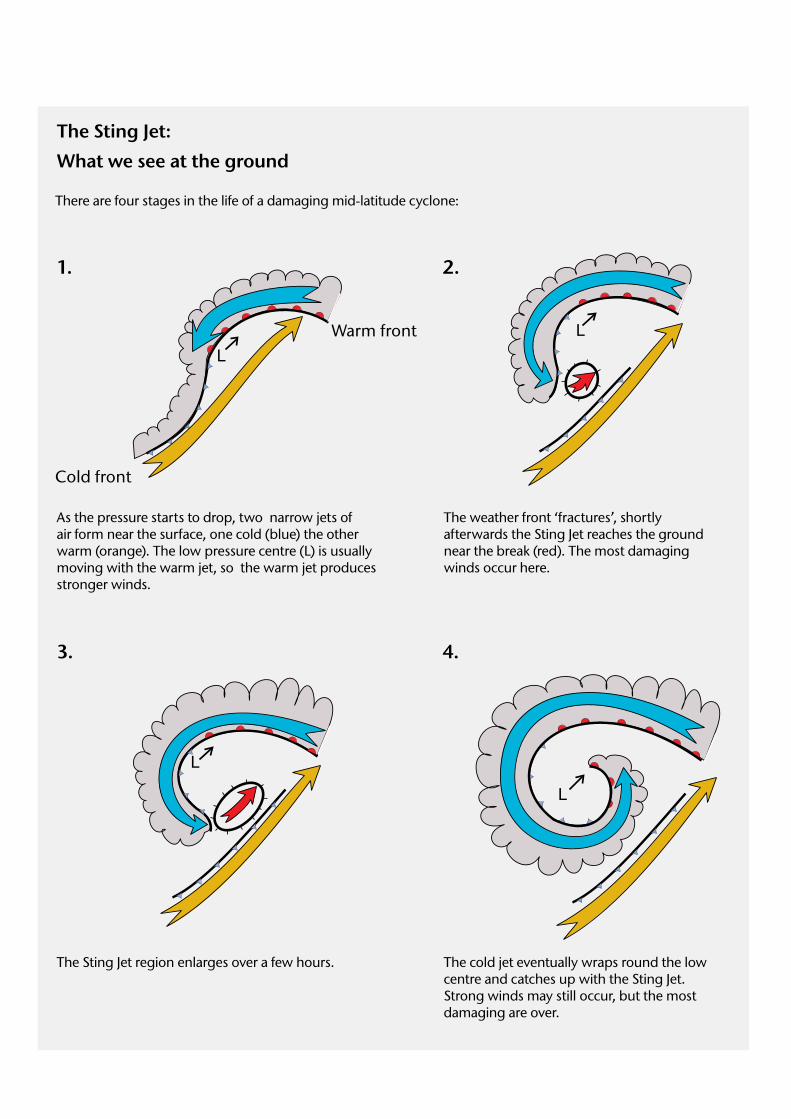
There are four stages in the life of a damaging mid-latitude cyclone:

The Sting Jet:

What we see at the ground

As the pressure starts to drop, two narrow jets of air form near the surface, one cold (blue) the other warm (orange). The low pressure centre (L) is usually moving with the warm jet, so the warm jet produces stronger winds.

L

L

Cold front

Warm front L

L

1. 2.

The weather front ‘fractures’, shortly afterwards the Sting Jet reaches the ground near the break (red). The most damaging winds occur here.

3. 4.

The Sting Jet region enlarges over a few hours. The cold jet eventually wraps round the low centre and catches up with the Sting Jet. Strong winds may still occur, but the most damaging are over.

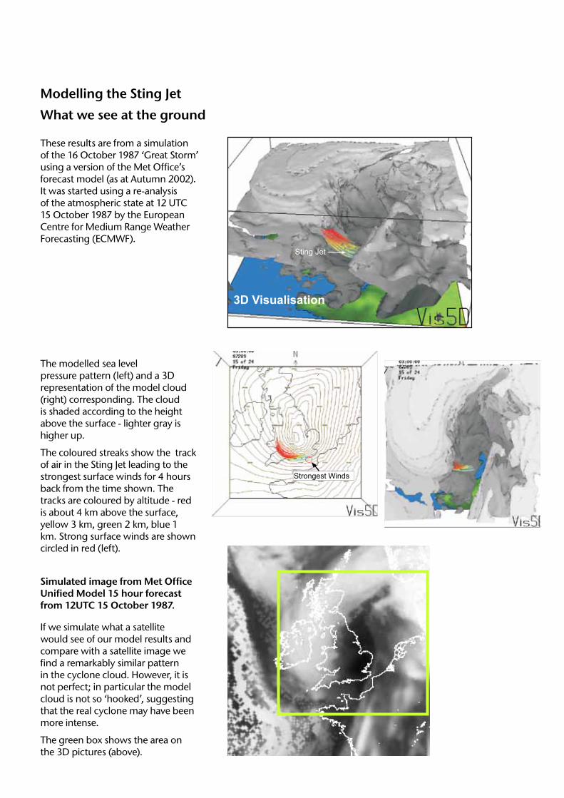
These results are from a simulation of the 16 October 1987 ‘Great Storm’ using a version of the Met Office’s forecast model (as at Autumn 2002).It was started using a re-analysis of the atmospheric state at 12 UTC 15 October 1987 by the European Centre for Medium Range Weather Forecasting (ECMWF).

2.

4.

Modelling the Sting Jet

What we see at the ground

The Sting Jet :Forecasting the Damaging Winds in European Cyclones

What is the Sting Jet?

Low pressure areas:

Experience has shown that:

We now know that:

���

�

�

�

�

�

�

�

Have well understood causes.Sometimes produce very strong windsAre generally well represented by ourweather forecast models.

The most damaging winds occur in a verysmall region, perhaps only 50 km across.This is close to the ‘tail’ of the ‘head’ of cloudthat wraps around the low pressure centre.Hence the ‘sting in the tail’ of the cyclone.

The ‘sting in the tail’ is produced by a distinctjet of air- the ‘Sting Jet’.It starts out 3 or 4 kilometres above theground and descends over 3 or 4 hours.Snow and rain falling into it evaporate andcool it as it descends, helping to accelerateit to high speeds.It can accelerate to more than 100 mph

The cold jet eventually wraps round the lowcentre and catches up with the Sting Jet.Strong winds may still occur, but the mostdamaging are over.

The Sting Jet region enlarges over a few hours.

The weather front ‘fractures’, shortlyafterwards the Sting Jet reaches the groundnear the break (red). The most damagingwinds occur here.

As the pressure starts to drop, two narrow jetsof air form near the surface, one cold (blue) theother warm (orange). The low pressure centre(L) is usually moving with the warm jet, so thewarm jet produces stronger winds

The Sting Jet:What we see at the ground.Four stages in the a damaging mid-latitude cyclonelife of

The cyclone forms on a weather front separating warm and cold air.The air flow is shown as if we were moving with the cyclone.

L

L

L

L

(a)

(c)

(b)

(d)

Warm front

Cold front

The ‘Great Storm’ of 1987

The famous ‘Great Storm’ cut a swathe of damageacross South-east England in the early hours of the16th October 1987. It was a good example of a stormwith a ’Sting Jet’.

The satellite image below shows the pattern of cloudjust before the strongest winds hit the south coast ofKent and Sussex near the ‘tail’ of the hook-shapedcloud wrapping round the cyclone. The red arrowshows the approximate path of the Sting Jet.

METEOSAT infra-red image03UTC 16 October 1987

SimulationModelling the Sting Jet

If we simulate what a satellite would see of ourmodel results and compare with a satellite image wefind a remarkably similar pattern in the cyclonecloud. However, it is not perfect; in particular themodel cloud is not so ‘hooked’, suggesting that thereal cyclone may have been more intense.The red box shows the area on the 3D pictures (left)

The modelled

track of air in the Sting Jet leading to thestrongest surface winds for 4 hours back from the time shown. Thetracks are coloured by altitude - red is about 4 km above the surface,yellow 3 km, green 2 km, blue 1 km. Strong surface winds are showncircled in red (left).

sea level pressure pattern (left) and a 3D representationof the model cloud (right) corresponding. The cloud is shaded accordingto the height above the surface - lighter gray is higher up.

The coloured streaks show the

Strongest Winds

Simulated image fromMet Office Unified Model

15 hour forecast from12UTC 15 October 1987

Why do we need to understand the StingJet?

We need to understand why the Sting Jet forms to make sureour model can represent it well.

We now know that we need:

1) To capture the width of the Sting Jet (about 50 km)

2) To capture the depth of the Sting Jet (about 1 km)

3) To capture the evaporation of snow (as it falls about 500 m).

3) To capture the interaction of the Sting Jet with the air flowingnear the surface.

Our current global forecast model has a horizontal gridlengthof about 60 km over the UK and has 38 levels going up tonearly 40 km. It does a good job of warning of strong winds,but predicts peak gusts of only about 60 knots (70 mph)(right). It predicts no Sting Jet.

A version of the model run over a region of about 3000 km x3000 km and with 90 levels produces a Sting Jet and does amuch better job, predicting gusts above 80 knots (95 mph).

Predicted peak wind gusts at 03 UTC 16thOctober 1987 during the ‘Great Storm’ using amodel with 12 km resolution and 90 levels. Themodel predicts more than 80 knots (about 95mph) in a region just crossing the south coast.

Predicted wind gusts at 03 UTCduring the ‘Great Storm’ using a model

with 60 km resolution, 38 levels.

16th October1987

The modelpredicts a large area of strong winds peakingat more than 60 knots (about 70 mph) in aregion just crossing the south coast.

Wind speeds measured at Shoreham bySea registered a gust of almost 100 knots(about 110 mph) just before the instrumentfailed. The model is better but still notperfect!

Anemometer Breaks!

3D Visualisation

Acknowledgement: This work wasperformed in collaboration with Prof. KeithBrowning at the Joint Centre for MesoscaleMeteorology, University of Reading

These results are from a simulation of the 16 October1987 ‘Great Storm’ using a version of the Met Office’sforecast model (as at Autumn 2002).It was started using are-analysis of the atmospheric state at 12 UTC 15October 1987 by the European Centre for Medium RangeWeather Forecasting (ECMWF).

Sting Jet

The Sting Jet :Forecasting the Damaging Winds in European Cyclones

What is the Sting Jet?

Low pressure areas:

Experience has shown that:

We now know that:

���

�

�

�

�

�

�

�

Have well understood causes.Sometimes produce very strong windsAre generally well represented by ourweather forecast models.

The most damaging winds occur in a verysmall region, perhaps only 50 km across.This is close to the ‘tail’ of the ‘head’ of cloudthat wraps around the low pressure centre.Hence the ‘sting in the tail’ of the cyclone.

The ‘sting in the tail’ is produced by a distinctjet of air- the ‘Sting Jet’.It starts out 3 or 4 kilometres above theground and descends over 3 or 4 hours.Snow and rain falling into it evaporate andcool it as it descends, helping to accelerateit to high speeds.It can accelerate to more than 100 mph

The cold jet eventually wraps round the lowcentre and catches up with the Sting Jet.Strong winds may still occur, but the mostdamaging are over.

The Sting Jet region enlarges over a few hours.

The weather front ‘fractures’, shortlyafterwards the Sting Jet reaches the groundnear the break (red). The most damagingwinds occur here.

As the pressure starts to drop, two narrow jetsof air form near the surface, one cold (blue) theother warm (orange). The low pressure centre(L) is usually moving with the warm jet, so thewarm jet produces stronger winds

The Sting Jet:What we see at the ground.Four stages in the a damaging mid-latitude cyclonelife of

The cyclone forms on a weather front separating warm and cold air.The air flow is shown as if we were moving with the cyclone.

L

L

L

L

(a)

(c)

(b)

(d)

Warm front

Cold front

The ‘Great Storm’ of 1987

The famous ‘Great Storm’ cut a swathe of damageacross South-east England in the early hours of the16th October 1987. It was a good example of a stormwith a ’Sting Jet’.

The satellite image below shows the pattern of cloudjust before the strongest winds hit the south coast ofKent and Sussex near the ‘tail’ of the hook-shapedcloud wrapping round the cyclone. The red arrowshows the approximate path of the Sting Jet.

METEOSAT infra-red image03UTC 16 October 1987

SimulationModelling the Sting Jet

If we simulate what a satellite would see of ourmodel results and compare with a satellite image wefind a remarkably similar pattern in the cyclonecloud. However, it is not perfect; in particular themodel cloud is not so ‘hooked’, suggesting that thereal cyclone may have been more intense.The red box shows the area on the 3D pictures (left)

The modelled

track of air in the Sting Jet leading to thestrongest surface winds for 4 hours back from the time shown. Thetracks are coloured by altitude - red is about 4 km above the surface,yellow 3 km, green 2 km, blue 1 km. Strong surface winds are showncircled in red (left).

sea level pressure pattern (left) and a 3D representationof the model cloud (right) corresponding. The cloud is shaded accordingto the height above the surface - lighter gray is higher up.

The coloured streaks show the

Strongest Winds

Simulated image fromMet Office Unified Model

15 hour forecast from12UTC 15 October 1987

Why do we need to understand the StingJet?

We need to understand why the Sting Jet forms to make sureour model can represent it well.

We now know that we need:

1) To capture the width of the Sting Jet (about 50 km)

2) To capture the depth of the Sting Jet (about 1 km)

3) To capture the evaporation of snow (as it falls about 500 m).

3) To capture the interaction of the Sting Jet with the air flowingnear the surface.

Our current global forecast model has a horizontal gridlengthof about 60 km over the UK and has 38 levels going up tonearly 40 km. It does a good job of warning of strong winds,but predicts peak gusts of only about 60 knots (70 mph)(right). It predicts no Sting Jet.

A version of the model run over a region of about 3000 km x3000 km and with 90 levels produces a Sting Jet and does amuch better job, predicting gusts above 80 knots (95 mph).

Predicted peak wind gusts at 03 UTC 16thOctober 1987 during the ‘Great Storm’ using amodel with 12 km resolution and 90 levels. Themodel predicts more than 80 knots (about 95mph) in a region just crossing the south coast.

Predicted wind gusts at 03 UTCduring the ‘Great Storm’ using a model

with 60 km resolution, 38 levels.

16th October1987

The modelpredicts a large area of strong winds peakingat more than 60 knots (about 70 mph) in aregion just crossing the south coast.

Wind speeds measured at Shoreham bySea registered a gust of almost 100 knots(about 110 mph) just before the instrumentfailed. The model is better but still notperfect!

Anemometer Breaks!

3D Visualisation

Acknowledgement: This work wasperformed in collaboration with Prof. KeithBrowning at the Joint Centre for MesoscaleMeteorology, University of Reading

These results are from a simulation of the 16 October1987 ‘Great Storm’ using a version of the Met Office’sforecast model (as at Autumn 2002).It was started using are-analysis of the atmospheric state at 12 UTC 15October 1987 by the European Centre for Medium RangeWeather Forecasting (ECMWF).

Sting Jet

The Sting Jet :Forecasting the Damaging Winds in European Cyclones

What is the Sting Jet?

Low pressure areas:

Experience has shown that:

We now know that:

���

�

�

�

�

�

�

�

Have well understood causes.Sometimes produce very strong windsAre generally well represented by ourweather forecast models.

The most damaging winds occur in a verysmall region, perhaps only 50 km across.This is close to the ‘tail’ of the ‘head’ of cloudthat wraps around the low pressure centre.Hence the ‘sting in the tail’ of the cyclone.

The ‘sting in the tail’ is produced by a distinctjet of air- the ‘Sting Jet’.It starts out 3 or 4 kilometres above theground and descends over 3 or 4 hours.Snow and rain falling into it evaporate andcool it as it descends, helping to accelerateit to high speeds.It can accelerate to more than 100 mph

The cold jet eventually wraps round the lowcentre and catches up with the Sting Jet.Strong winds may still occur, but the mostdamaging are over.

The Sting Jet region enlarges over a few hours.

The weather front ‘fractures’, shortlyafterwards the Sting Jet reaches the groundnear the break (red). The most damagingwinds occur here.

As the pressure starts to drop, two narrow jetsof air form near the surface, one cold (blue) theother warm (orange). The low pressure centre(L) is usually moving with the warm jet, so thewarm jet produces stronger winds

The Sting Jet:What we see at the ground.Four stages in the a damaging mid-latitude cyclonelife of

The cyclone forms on a weather front separating warm and cold air.The air flow is shown as if we were moving with the cyclone.

L

L

L

L

(a)

(c)

(b)

(d)

Warm front

Cold front

The ‘Great Storm’ of 1987

The famous ‘Great Storm’ cut a swathe of damageacross South-east England in the early hours of the16th October 1987. It was a good example of a stormwith a ’Sting Jet’.

The satellite image below shows the pattern of cloudjust before the strongest winds hit the south coast ofKent and Sussex near the ‘tail’ of the hook-shapedcloud wrapping round the cyclone. The red arrowshows the approximate path of the Sting Jet.

METEOSAT infra-red image03UTC 16 October 1987

SimulationModelling the Sting Jet

If we simulate what a satellite would see of ourmodel results and compare with a satellite image wefind a remarkably similar pattern in the cyclonecloud. However, it is not perfect; in particular themodel cloud is not so ‘hooked’, suggesting that thereal cyclone may have been more intense.The red box shows the area on the 3D pictures (left)

The modelled

track of air in the Sting Jet leading to thestrongest surface winds for 4 hours back from the time shown. Thetracks are coloured by altitude - red is about 4 km above the surface,yellow 3 km, green 2 km, blue 1 km. Strong surface winds are showncircled in red (left).

sea level pressure pattern (left) and a 3D representationof the model cloud (right) corresponding. The cloud is shaded accordingto the height above the surface - lighter gray is higher up.

The coloured streaks show the

Strongest Winds

Simulated image fromMet Office Unified Model

15 hour forecast from12UTC 15 October 1987

Why do we need to understand the StingJet?

We need to understand why the Sting Jet forms to make sureour model can represent it well.

We now know that we need:

1) To capture the width of the Sting Jet (about 50 km)

2) To capture the depth of the Sting Jet (about 1 km)

3) To capture the evaporation of snow (as it falls about 500 m).

3) To capture the interaction of the Sting Jet with the air flowingnear the surface.

Our current global forecast model has a horizontal gridlengthof about 60 km over the UK and has 38 levels going up tonearly 40 km. It does a good job of warning of strong winds,but predicts peak gusts of only about 60 knots (70 mph)(right). It predicts no Sting Jet.

A version of the model run over a region of about 3000 km x3000 km and with 90 levels produces a Sting Jet and does amuch better job, predicting gusts above 80 knots (95 mph).

Predicted peak wind gusts at 03 UTC 16thOctober 1987 during the ‘Great Storm’ using amodel with 12 km resolution and 90 levels. Themodel predicts more than 80 knots (about 95mph) in a region just crossing the south coast.

Predicted wind gusts at 03 UTCduring the ‘Great Storm’ using a model

with 60 km resolution, 38 levels.

16th October1987

The modelpredicts a large area of strong winds peakingat more than 60 knots (about 70 mph) in aregion just crossing the south coast.

Wind speeds measured at Shoreham bySea registered a gust of almost 100 knots(about 110 mph) just before the instrumentfailed. The model is better but still notperfect!

Anemometer Breaks!

3D Visualisation

Acknowledgement: This work wasperformed in collaboration with Prof. KeithBrowning at the Joint Centre for MesoscaleMeteorology, University of Reading

These results are from a simulation of the 16 October1987 ‘Great Storm’ using a version of the Met Office’sforecast model (as at Autumn 2002).It was started using are-analysis of the atmospheric state at 12 UTC 15October 1987 by the European Centre for Medium RangeWeather Forecasting (ECMWF).

Sting Jet

The modelled sea level pressure pattern (left) and a 3D representation of the model cloud (right) corresponding. The cloud is shaded according to the height above the surface - lighter gray is higher up.

The coloured streaks show the track of air in the Sting Jet leading to the strongest surface winds for 4 hours back from the time shown. The tracks are coloured by altitude - red is about 4 km above the surface, yellow 3 km, green 2 km, blue 1 km. Strong surface winds are shown circled in red (left).

Simulated image from Met Office Unified Model 15 hour forecast from 12UTC 15 October 1987.

If we simulate what a satellite would see of our model results and compare with a satellite image we find a remarkably similar pattern in the cyclone cloud. However, it is not perfect; in particular the model cloud is not so ‘hooked’, suggesting that the real cyclone may have been more intense.

The green box shows the area on the 3D pictures (above).

03UTC 16/10/1987 from 12UTC 15/10/1987 10 m peak gust

40

40

40

40

40

40

50

50

50

60

5060

7080

40

4050

40

40

40

03UTC 16/10/1987 from 12UTC 15/10/1987 10 m peak gust

5W 0 5E

48N

50N

52N

54N

56N

40

40 50

50

50

40

40

60

Met OfficeFitzRoy Road, ExeterDevon, EX1 3PBUnited Kingdom

Tel: +44(0)1392 885680Email: renewables@metoffice.gov.ukwww.metoffice.gov.uk/renewables/windreview

Produced by the Met Office. © Crown copyright 2012 12/0541Met Office and the Met Office logo are registered trademarks

We need to understand why the Sting Jet forms to make sure our model can represent it well.

We now know that we need:

1) To capture the width of the Sting Jet (about 50 km)

2) To capture the depth of the Sting Jet (about 1 km)

3) To capture the evaporation of snow (as it falls about 500 m).

4) To capture the interaction of the Sting Jet with the air flowing near the surface.

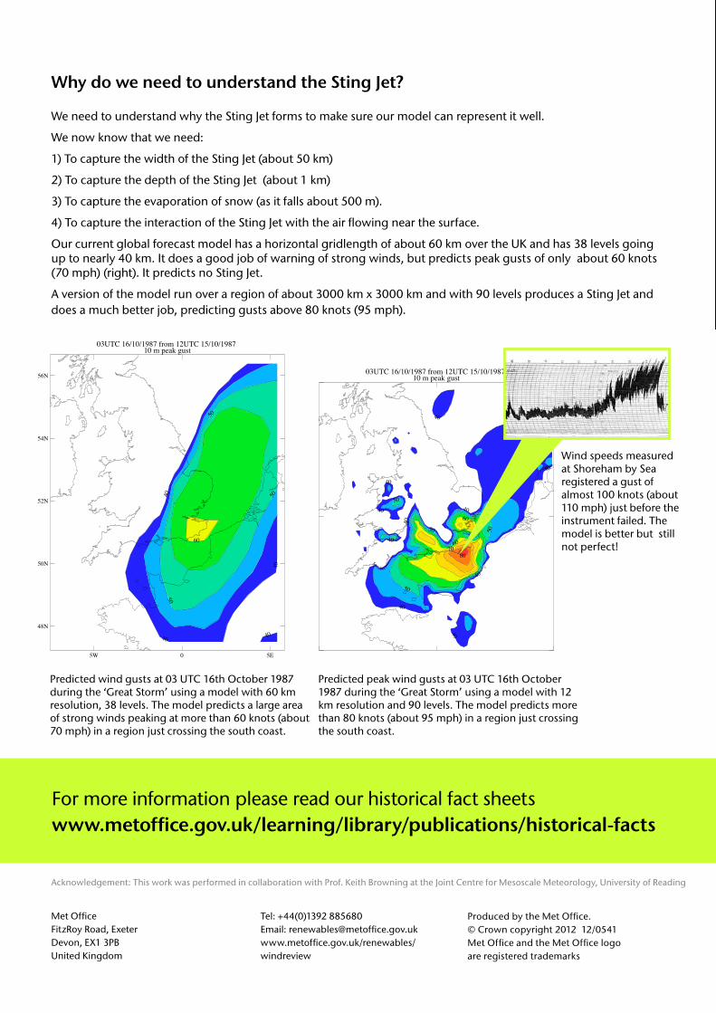
Our current global forecast model has a horizontal gridlength of about 60 km over the UK and has 38 levels going up to nearly 40 km. It does a good job of warning of strong winds, but predicts peak gusts of only about 60 knots (70 mph) (right). It predicts no Sting Jet.

A version of the model run over a region of about 3000 km x 3000 km and with 90 levels produces a Sting Jet and does a much better job, predicting gusts above 80 knots (95 mph).

For more information please read our historical fact sheets www.metoffice.gov.uk/learning/library/publications/historical-facts

Why do we need to understand the Sting Jet?

Predicted wind gusts at 03 UTC 16th October 1987 during the ‘Great Storm’ using a model with 60 km resolution, 38 levels. The model predicts a large area of strong winds peaking at more than 60 knots (about 70 mph) in a region just crossing the south coast.

Predicted peak wind gusts at 03 UTC 16th October 1987 during the ‘Great Storm’ using a model with 12 km resolution and 90 levels. The model predicts more than 80 knots (about 95 mph) in a region just crossing the south coast.

Wind speeds measured at Shoreham by Sea registered a gust of almost 100 knots (about 110 mph) just before the instrument failed. The model is better but still not perfect!

Acknowledgement: This work was performed in collaboration with Prof. Keith Browning at the Joint Centre for Mesoscale Meteorology, University of Reading