Does mesoscale instability control sting jet variability?

Neil Hart, Suzanne Gray and Peter Clark

Martínez-Alvarado et al 2014, MWR

Instability and Predictability

Convective Instability

SymmetricInstability

BaroclinicInstability

~100km~6hours

~1000km~day

~1km~30mins

Courtesy: ECMWF

St Jude Forecast:Global Ensemble

Courtesy: MetOffice

St Jude Forecast: MetOffice 4km

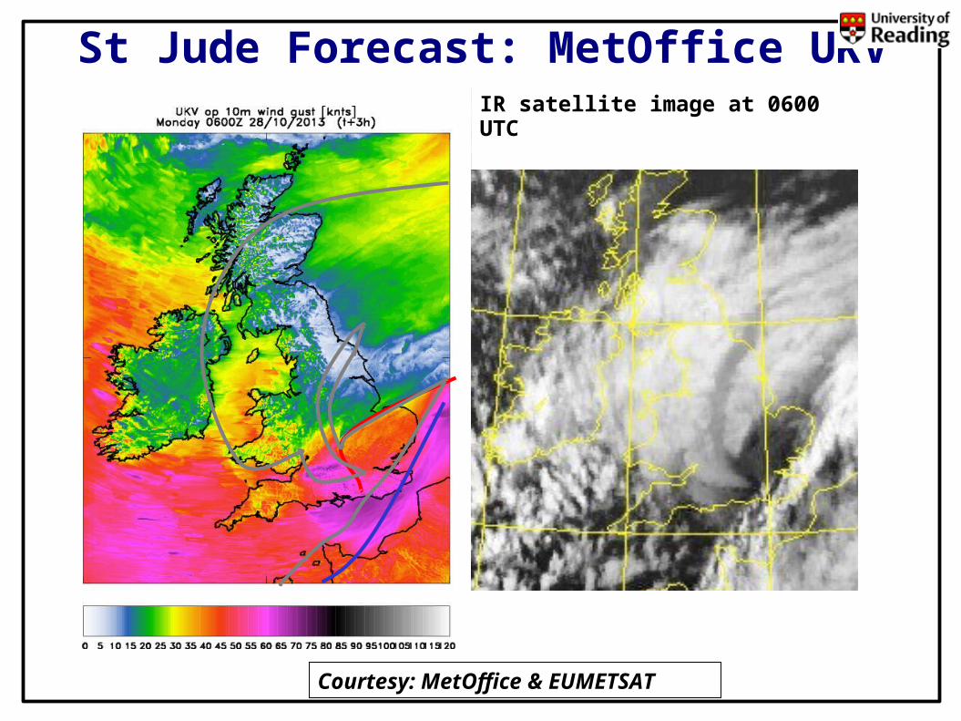
IR satellite image at 0600 UTC

Courtesy: MetOffice & EUMETSAT

St Jude Forecast: MetOffice UKV

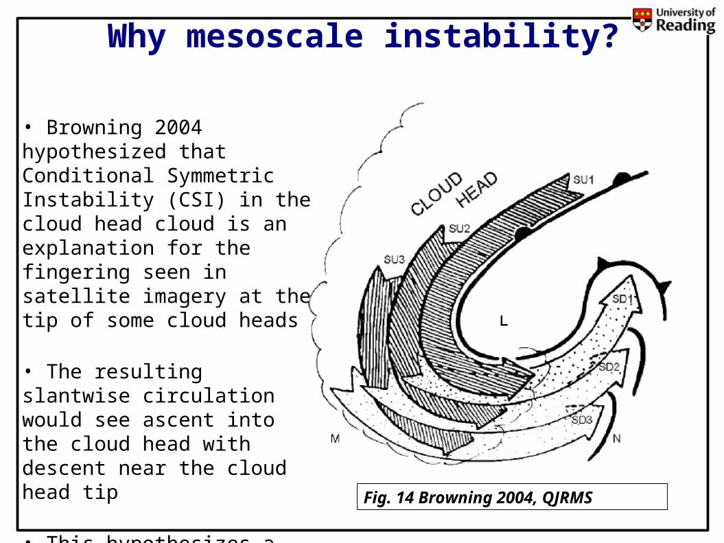
Fig. 14 Browning 2004, QJRMS

Why mesoscale instability?

• Browning 2004 hypothesized that Conditional Symmetric Instability (CSI) in the cloud head cloud is an explanation for the fingering seen in satellite imagery at the tip of some cloud heads

• The resulting slantwise circulation would see ascent into the cloud head with descent near the cloud head tip

• This hypothesizes a mechanism for sting jet descents, as seen in 1987 Great Storm

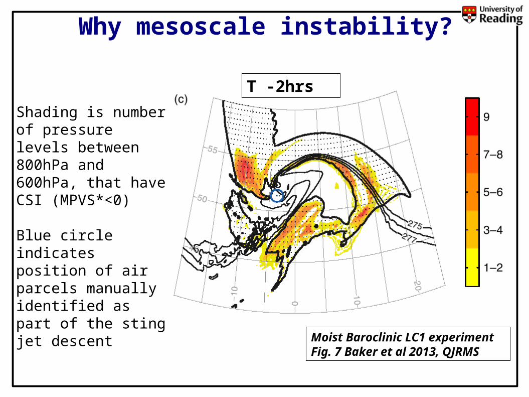
Moist Baroclinic LC1 experimentFig. 7 Baker et al 2013, QJRMS

Why mesoscale instability?

Shading is number of pressure levels between 800hPa and 600hPa, that have CSI (MPVS*<0)

Blue circle indicates position of air parcels manually identified as part of the sting jet descent

T -10hrs

Why mesoscale instability?

T -6hrs

Moist Baroclinic LC1 experimentFig. 7 Baker et al 2013, QJRMS

Shading is number of pressure levels between 800hPa and 600hPa, that have CSI (MPVS*<0)

Blue circle indicates position of air parcels manually identified as part of the sting jet descent

Why mesoscale instability?

T -2hrs

Moist Baroclinic LC1 experimentFig. 7 Baker et al 2013, QJRMS

Shading is number of pressure levels between 800hPa and 600hPa, that have CSI (MPVS*<0)

Blue circle indicates position of air parcels manually identified as part of the sting jet descent

Friedhelm, Robert and Ulli

Martínez-Alvarado et al 2014, MWR

Smart & Browning 2013

Friedhelm 8 Dec ‘11 Robert 27 Dec ’11 Ulli 3 Jan ‘12

Identified with DSCAPE diagnostic applied to ERA-Interim (after Martínez-Alvarado 2012)

Courtesy: EUMETSAT, Sat24.com

Cyclone Robert

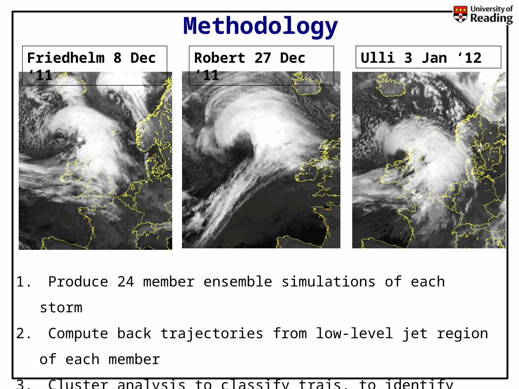
MethodologyFriedhelm 8 Dec ‘11 Robert 27 Dec ’11 Ulli 3 Jan ‘12

1. Produce 24 member ensemble simulations of each storm

2. Compute back trajectories from low-level jet region of each member

3. Cluster analysis to classify trajs. to identify descending airstreams

4. Explore link between these descents and CSI across ensemble

• MetOffice Unified Model vn8.2

• MOGREPS-Global ETKF

24 Init. Pert. Members

(Bowler et al, 2008)

• MOGREPS-Regional

• N. Atl. & Europe Domain

• 12km, 70 Levels

• All storms initialised at 18 UTC

the day before maximum intensity

• Results analysed further are T+10 to T+24 forecasts

Model Setup

Synoptic Overview

Synoptic Overview

Small spread in synoptic scale evolution between ensemble members:

Good, since can now focus on mesoscale differences

Compute Back Trajectories

Control Run from Cyclone Robert ensemble

Compute Back Trajectories

Cloud Top Temperature

Control Run from Cyclone Robert ensemble

850hPa 45m/s Isotach

Compute Back Trajectories

Control Run from Cyclone Robert ensemble

Trajectories Computed with Lagranto (Wernli & Davies, 1997)

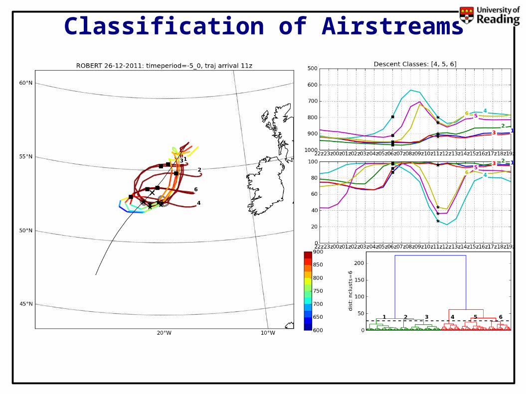
Classification of Airstreams

Ward’s Hierarchical Clustering Algorthim

Use Relative Humidity to remove descents that started outside cloud head

Identify class means that descend Cluster Class Mean

Trajectories: Each trajectory described by x,y, P, θw for 5 hours preceding arrival in low-level jet

Classification of Airstreams

Ward’s Hierarchical Clustering Algorthim

Use Relative Humidity to remove descents that started outside cloud head

Identify class means that descend

Classification of Airstreams

Use Relative Humidity to remove descents that started outside cloud head

Identify class means that descend

Classification of Airstreams

Use Relative Humidity to remove descents that started outside cloud head

Classification of Airstreams

Classification of Airstreams

Each Class contains a population of individual trajectories that arrive at given time.

Next slideSize of these populations are gathered for all descent classes at all times for each ensemble member

# of Traj. Arriving in LLJ

160

0

# of Traj. Arriving in LLJ

160

0

Majority of of ensemble members have peak in # trajs at 12UTC

Ensemble Sensitivity

Control run cloud head Control run 281K θw 850hpa

Interpret as change in # trajs for 1 s.d change in CSI metric

X

Ensemble Sensitivity

Methodology after Torn & Hakim 2008

X

Ensemble Sensitivity

Methodology after Torn & Hakim 2008

X

Ensemble Sensitivity

Methodology after Torn & Hakim 2008

X

Ensemble Sensitivity

Methodology after Torn & Hakim 2008

X

Consistent synoptic development across ensemble

Considerable variability in mesoscale wind features

Demonstrated method to classify descending airstreams

Large variability in number of descending trajectories across

ensemble

Does mesoscale instability control sting jet variability?

Strength of sting jet descent is associated

with CSI in the cloud head

(in Robert as simulated with MetUM)

Conclusions

Cyclone Friedhelm

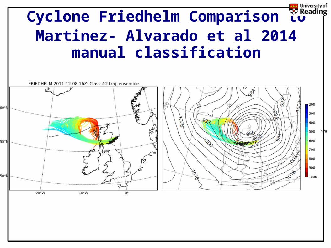
Cyclone Friedhelm Comparison toMartinez- Alvarado et al 2014 manual

classification

Ensemble Sensitivity

CSI across ensemble

# tr

ajs

If correlation > threshold(0.5 used here), good!

Ensemble Sensitivity

CSI across ensemble

# tr

ajs

∆x

∆y

Calculate Gradient

Ensemble Sensitivity

CSI across ensemble

# tr

ajs

∆x

∆y

Ens. Sensitivity = ∆y (∆x = 1 s.d.)