Embed Size (px)
Citation preview
THE SCHWARZSCHILD PROBLEM IN ASTROPHYSICS
CRISTINA STOICAInstitute for Gravitation and Space Sciences, Gravitational Research Laboratory, Str. Mendeleev
21-25, 70168 Bucharest, Romania
VASILE MIOCAstronomical Institute of the Romanian Academy, Astronomical Observatory Cluj-Napoca, Str.
Ciresilor 19, 3400 Cluj-Napoca, Romania
(Received 25 September, 1996; accepted 14 March, 1997)
Abstract. The Schwarzschild problem (the two-body problem associated to a potential of the formA=r + B=r
3) has been qualitatively investigated in an astrophysical framework, exemplified bytwo likely situations: motion of a particle in the photogravitational field of an oblate, rotating star,or in that of a star which generates a Schwarzschild field. Using McGehee-type transformations,regularized equations of motion are obtained, and the collision singularity is blown up and replacedby the collision manifold � (a torus) pasted on the phase space. The flow on � is fully characterized.Then, reducing the 4D phase space to dimension 2, the global flow in the phase plane is depicted forall possible values of the energy and for all combinations of nonzero A and B. Each phase trajectoryis interpreted in terms of physical motion, obtaining in this way a telling geometric and physicalpicture of the model.
1. Introduction
The theory of orbits in a force field characterized by a potential
U(r) = A=r +B=r3 (1)
(r = distance of a particle to the field source; A;B = constants) constitutesan extensively discussed subject. This theory, which models concrete problemsbelonging to astrophysics, stellar dynamics, celestial mechanics, astrodynamics,cosmogony, etc., was approached by various methods, both qualitative and (espe-cially) quantitative. To bring the problem in the realm of astrophysics, it is suffi-ciently significant in our opinion to mention two very likely situations that relevantto this model. Consider an oblate, uniformly rotating star of mass M , luminosityL�, equatorial radius R, oblateness ", and angular velocity !. Also consider aspherical particle of unit mass, constant albedo, and cross section �, moving atdistance r in the equatorial plane of this one. The force acting on the particle comesfrom a potential of the form (1) with
A = GM � �L�=(4�c); B = JGMR2=3; (2)
where J = "� !2R3=(2GM), G stands for the Newtonian gravitational constant,and c is the speed of light.
Astrophysics and Space Science 249: 161–173, 1997.c 1997 Kluwer Academic Publishers. Printed in Belgium.
GSB: 307 PIPS Nr.: 137580 SPACKAPas177.tex; 6/01/1998; 0:15; v.5; p.1
162 C. STOICA AND V. MIOC
The other situation is somewhat equivalent from a mathematical standpoint. Letnow the star be spherical and rotationless, but characterize its gravitational field bySchwarzschild’s metric. Taking also into account the radiative field, one is led to aBinet equation (cf., e.g., Eddington, 1923; Blaga and Mioc, 1992) correspondingagain to a potential of the form (1) in which
A = GM � �L�=(4�c); B = GMC2=c2; (3)
where C is the constant angular momentum.Many authors studied quantitatively the motion in such a field (see, e.g., Brum-
berg, 1972; Chandrasekhar, 1983; Damour and Schaefer, 1986), generally in a rel-ativistic context, showing that the analytic solution of the problem can be obtainedin closed form by means of elliptic functions. But, on the one hand, the analyticform of these solutions hides the general geometric properties of the model. Onthe other hand, considering only the gravitational field, one is confined to A > 0,B > 0 (Schwarzschild case) or A > 0, B < 0 (artificial satellite problem, forinstance).
As to the rather few qualitative approaches, they dealt mainly with the regular-ization of motion equations (see, e.g., Saari, 1974; Belenkii, 1981; Szebehely andBond, 1983; Cid et al., 1983). In addition, the quoted authors used only Sundman-type transformations of time.
The aim of this paper is to study qualitatively the problem for any A 6= 0,B 6= 0 (the case A = 0 is recoverable in a McGehee’s (1981) paper, while B = 0is trivial), and to provide a complete geometric and physical description of theorbits. We have to specify that the motion will be studied within the framework ofthe two-body problem (in the point mass approximation) associated to the potential(1), which we shall hereafter call the Schwarzschild problem.
We shall resort to the powerful tool of McGehee-type transformations of thesecond kind, little used among the (astro)physicists. By means of this technique weblow up the collision singularity at the origin, and obtain regularized equations ofmotion. In this way, a collision manifold � is pasted, instead of the singularity, onthe phase space. We describe the flow on �; due to the continuity with respect toinitial data, the study of this (fictitious) flow provides informations about the localmotion near collision.
Next, exploiting successively the rotational symmetry of the global flow, and thefirst integral of angular momentum, we restrict the 4-dimensional full phase space tothe 3-dimensional reduced phase space (RPS), then to dimension 2 (the phase plane– PP). Regarding the energy as a parameter, the energy integral (characterized bythe constant h) is plotted in PP for the whole interplay among the field parameters(A and B) and h, allowing a wide description of the phase plane structure. Everypossible orbit in PP is interpreted in terms of physical motion. In this way, theastrophysical Schwarzschild problem is widely depicted both geometrically andphysically.
as177.tex; 6/01/1998; 0:15; v.5; p.2

THE SCHWARZSCHILD PROBLEM IN ASTROPHYSICS 163
2. Equations of Motion and First Integrals
Since the potential (1) is central, the motion of the particle is confined to a plane.Consider hence the field source M fixed at the origin of this plane R2, and write(1) in the form
U(q) = A=jqj+B=jqj3; (4)
where q = (q1; q2) 2 R2 is the position (or configuration) of the particle, andj � j denotes the Euclidean norm. Introducing the momentum vector p = _q, p =(p1; p2) 2 R2, the motion is described by the coupled equations
_q = p;
_p = rU(q);(5)
which define a vector field on the phase space Q � P, where Q = R2nf(0; 0)g isthe configuration space, and P = R2 is the momentum space.
Denoting by T (p) = jpj2=2 the kinetic energy of the particle, the Hamiltonianfunction H(q;p) = T (p)� U(q) has the property
H(q;p) = h=2 = constant, (6)
namely it is a first integral of the system (called the integral of energy;h is the energyconstant). The field being central, the angular momentum L(q;p) = q1p2 � q2p1
is conserved, and we have another first integral
L(q;p) = C = constant, (7)
where C is the constant of angular momentum.Explicitly, the equations of motion are
_q = p;
_p = �(A=jqj3 +B=jqj5)q;(8)
with the energy relation
jpj2 � 2A=jqj � 2B=jqj3 = h: (9)
3. McGehee’s Transformations
The potential (4) has an isolated singularity at the origin q = (0; 0), which, asshown by Saari (1974), corresponds to the collision particle-centre. To remove itand to regularize Equations (8), we shall resort to McGehee-type transformationsof the second kind (McGehee, 1974). For this purpose we perform successively thetransformations:
as177.tex; 6/01/1998; 0:15; v.5; p.3
164 C. STOICA AND V. MIOC
r = jqj;
� = arctan(q2=q1);
u = _r = (q1p1 + q2p2)=jqj;
v = r _� = (q1p2 � q2p1)=jqj;
(10)
(which introduce standard polar coordinates);
x = r3=2u; y = r3=2v; (11)
(which scale down the components of velocity); and
dt = r5=2ds; (12)
(which rescales the time). By Equations (10)–(12), which all define real analyticdiffeomorphisms, the equations of motion (8) become
r0 = rx;
�0 = y;
x0 = 32x
2 + y2 �Ar2 � 3B;
y0 = 12xy;
(13)
where primes mark differentiation with respect to the new (fictitious) time variables, and we maintained by abuse the same notations for the new functions of s.
Also, using the transformations (10)–(11), the first integrals of energy (9) andangular momentum (7) read respectively
x2 + y2 = hr3 + 2Ar2 + 2B; (14)
y2 = C2r: (15)
Both the equations of motion (13) and the first integrals (14)–(15) are now welldefined for the boundary r = 0. This means that the phase space can be extendedanalytically to contain the manifold f(r; �; x; y)jr = 0g, which is invariant underthe flow since r0 = 0 when r = 0. The relations (14) and (15) also extend smoothlyto this boundary. The flow on this invariant manifold, although deprived of physicalsignificance, provides valuable informations about near-collisional orbits (due tothe continuity of solutions with respect to the initial conditions).
4. The Collision Manifold and the Flow on it
Define the collision manifold� as being the intersection of the sets f(r; �; x; y)jr =0g and f(r; �; x; y)jx2 + y2 = hr3 + 2Ar2 + 2Bg. This intersection is the set
as177.tex; 6/01/1998; 0:15; v.5; p.4
THE SCHWARZSCHILD PROBLEM IN ASTROPHYSICS 165
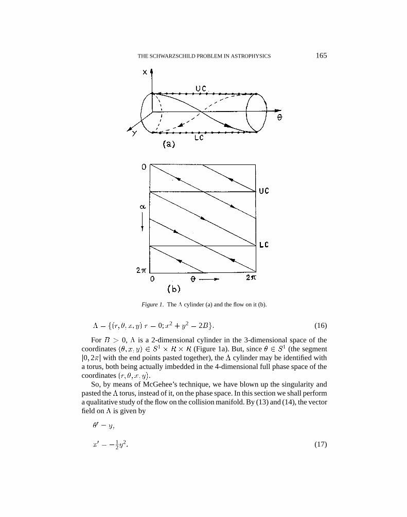
Figure 1. The � cylinder (a) and the flow on it (b).
� = f(r; �; x; y)jr = 0;x2 + y2 = 2Bg: (16)
For B > 0, � is a 2-dimensional cylinder in the 3-dimensional space of thecoordinates (�; x; y) 2 S1 � R � R (Figure 1a). But, since � 2 S1 (the segment[0; 2�] with the end points pasted together), the � cylinder may be identified witha torus, both being actually imbedded in the 4-dimensional full phase space of thecoordinates (r; �; x; y).
So, by means of McGehee’s technique, we have blown up the singularity andpasted the � torus, instead of it, on the phase space. In this section we shall performa qualitative study of the flow on the collision manifold. By (13) and (14), the vectorfield on � is given by
�0 = y;
x0 = �12y
2; (17)
as177.tex; 6/01/1998; 0:15; v.5; p.5
166 C. STOICA AND V. MIOC
y0 = 12xy
Equations (17) admit the fixed points (�; x; y) = (�0;�p
2B; 0) with �0 2 S1
arbitrary. In other words, there are two circles of degenerate equilibria on the �torus, at y = 0. Since, by (17), x0 < 0 for y 6= 0, all other orbits of the flow on� are heteroclinic and move from the upper circle (UC) x =
p2B to the lower
circle (LC) x = �p
2B. Introducing the angular variable � via x =p
2B sin�,y = �
p2B cos�, Equations (17) transform into
�0 = �p
2B cos�;
�0 = �pB=2 cos�;
(18)
which lead to d�=d� = 1=2. The flow on � in these coordinates is illustrated inFigure 1b.
By (15) one observes easily that all collisional orbits eject from UC or tend toLC. It is also clear that collisions can occur not only forC = 0 (as in the Newtonianmodel), but for C 6= 0, too (cf. Saari, 1974; McGehee, 1981; Diacu et al., 1995).
Also remark that for B = 0 (case which will not be considered here; seeSection 1) � reduces to a circle of degenerate equilibria (LC and UC identified).For B < 0, � is the empty set (that is, the motion is collision-free); Saari (1974)also established such a result, but within another framework and using anothermethod.
Finally notice, by (16), that, when � is nonempty (nonnegative B), it does notdepend on h, therefore every energy level shares this boundary.
5. The Global Flow
Observe that � does not appear explicitly in either regularized equations of motion(13) or first integrals (14) and (15). We can therefore reduce the full phase spaceof (r; �; x; y) to dimension 3 by factorizing the flow to S1; in this way we getthe reduced phase space of the coordinates (r; x; y) (hereafter RPS). Of course, asolution in RPS must be regarded as a manifold of solutions in full phase space.
We can further reduce RPS to dimension 2 by resorting to the integral ofangular momentum (15), which relates y to r. So we obtain the phase plane of thecoordinates (r; x) (hereafter PP). It is obvious that what we said above about theorbits in RPS is to be applied to the solutions in PP, too.
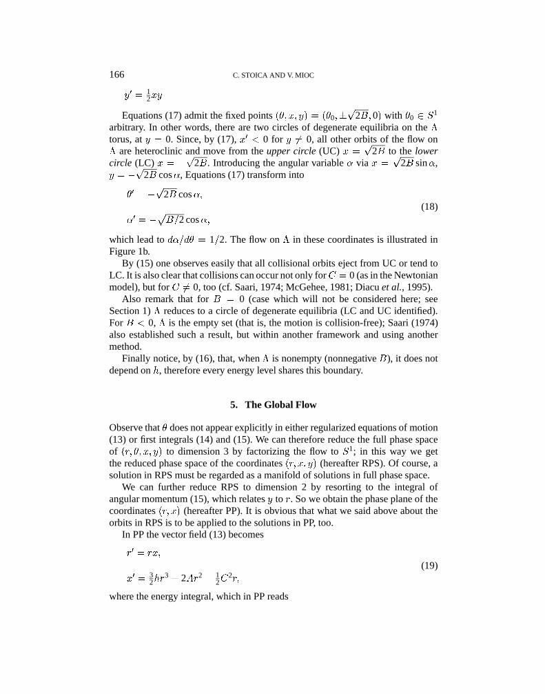
In PP the vector field (13) becomes
r0 = rx;
x0 = 32hr
3 + 2Ar2 � 12C
2r;
(19)
where the energy integral, which in PP reads
as177.tex; 6/01/1998; 0:15; v.5; p.6
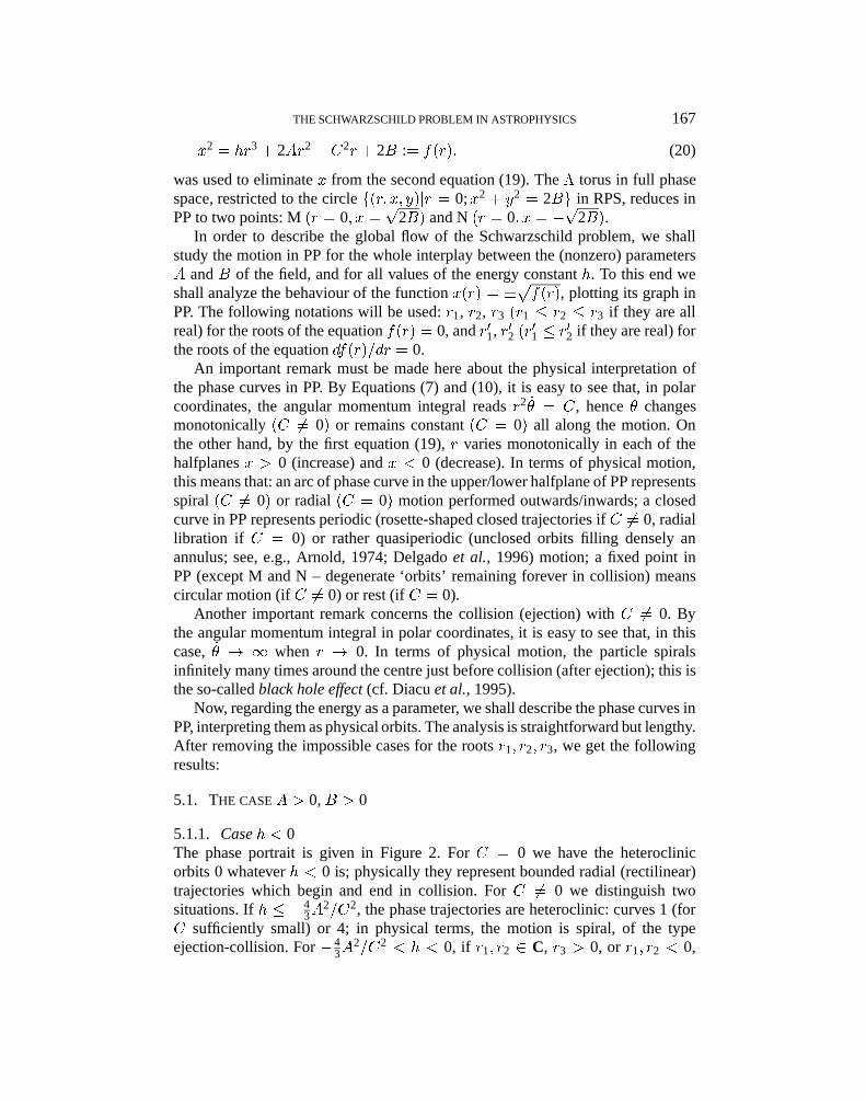
THE SCHWARZSCHILD PROBLEM IN ASTROPHYSICS 167
x2 = hr3 + 2Ar2 � C2r + 2B := f(r); (20)
was used to eliminate x from the second equation (19). The � torus in full phasespace, restricted to the circle f(r; x; y)jr = 0;x2 + y2 = 2Bg in RPS, reduces inPP to two points: M (r = 0; x =
p2B) and N (r = 0; x = �
p2B).
In order to describe the global flow of the Schwarzschild problem, we shallstudy the motion in PP for the whole interplay between the (nonzero) parametersA and B of the field, and for all values of the energy constant h. To this end weshall analyze the behaviour of the function x(r) = �
pf(r), plotting its graph in
PP. The following notations will be used: r1, r2, r3 (r1 � r2 � r3 if they are allreal) for the roots of the equation f(r) = 0, and r01, r02 (r01 � r02 if they are real) forthe roots of the equation df(r)=dr = 0.
An important remark must be made here about the physical interpretation ofthe phase curves in PP. By Equations (7) and (10), it is easy to see that, in polarcoordinates, the angular momentum integral reads r2 _� = C , hence � changesmonotonically (C 6= 0) or remains constant (C = 0) all along the motion. Onthe other hand, by the first equation (19), r varies monotonically in each of thehalfplanes x > 0 (increase) and x < 0 (decrease). In terms of physical motion,this means that: an arc of phase curve in the upper/lower halfplane of PP representsspiral (C 6= 0) or radial (C = 0) motion performed outwards/inwards; a closedcurve in PP represents periodic (rosette-shaped closed trajectories if C 6= 0, radiallibration if C = 0) or rather quasiperiodic (unclosed orbits filling densely anannulus; see, e.g., Arnold, 1974; Delgado et al., 1996) motion; a fixed point inPP (except M and N – degenerate ‘orbits’ remaining forever in collision) meanscircular motion (if C 6= 0) or rest (if C = 0).
Another important remark concerns the collision (ejection) with C 6= 0. Bythe angular momentum integral in polar coordinates, it is easy to see that, in thiscase, _� ! 1 when r ! 0. In terms of physical motion, the particle spiralsinfinitely many times around the centre just before collision (after ejection); this isthe so-called black hole effect (cf. Diacu et al., 1995).
Now, regarding the energy as a parameter, we shall describe the phase curves inPP, interpreting them as physical orbits. The analysis is straightforward but lengthy.After removing the impossible cases for the roots r1; r2; r3, we get the followingresults:
5.1. THE CASE A > 0, B > 0
5.1.1. Case h < 0The phase portrait is given in Figure 2. For C = 0 we have the heteroclinicorbits 0 whatever h < 0 is; physically they represent bounded radial (rectilinear)trajectories which begin and end in collision. For C 6= 0 we distinguish twosituations. If h � �4
3A2=C2, the phase trajectories are heteroclinic: curves 1 (for
C sufficiently small) or 4; in physical terms, the motion is spiral, of the typeejection-collision. For �4
3A2=C2 < h < 0, if r1; r2 2 C, r3 > 0, or r1; r2 < 0,
as177.tex; 6/01/1998; 0:15; v.5; p.7
168 C. STOICA AND V. MIOC
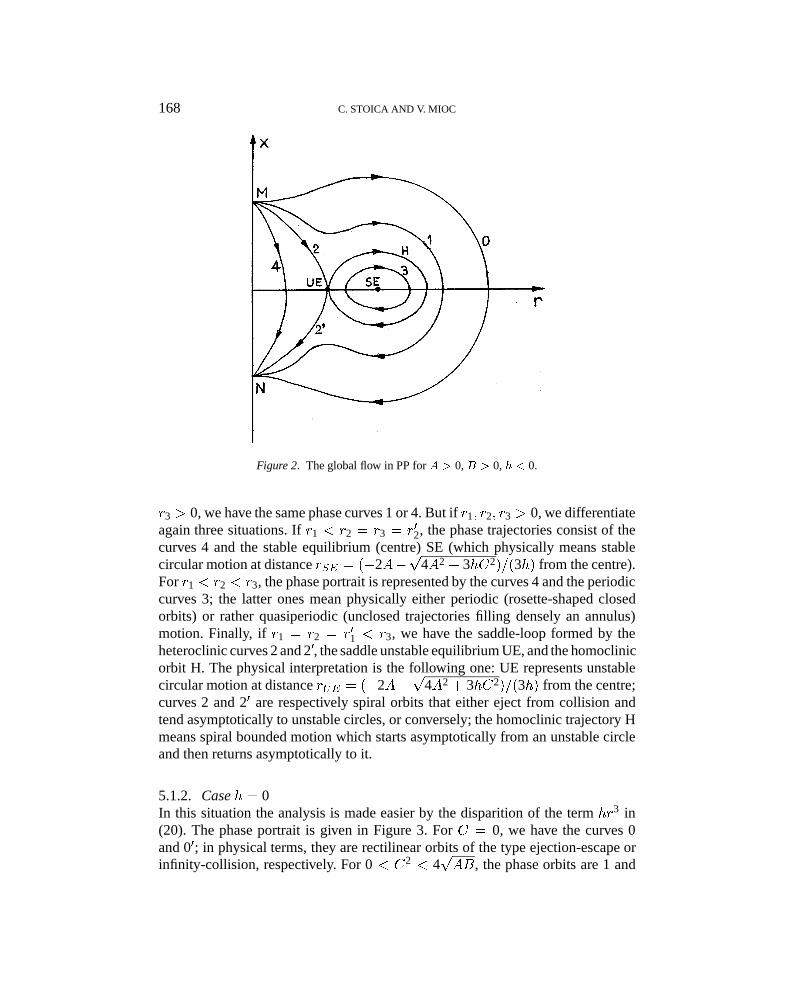
Figure 2. The global flow in PP for A > 0, B > 0, h < 0.
r3 > 0, we have the same phase curves 1 or 4. But if r1; r2; r3 > 0, we differentiateagain three situations. If r1 < r2 = r3 = r02, the phase trajectories consist of thecurves 4 and the stable equilibrium (centre) SE (which physically means stablecircular motion at distance rSE = (�2A�
p4A2 + 3hC2)=(3h) from the centre).
For r1 < r2 < r3, the phase portrait is represented by the curves 4 and the periodiccurves 3; the latter ones mean physically either periodic (rosette-shaped closedorbits) or rather quasiperiodic (unclosed trajectories filling densely an annulus)motion. Finally, if r1 = r2 = r01 < r3, we have the saddle-loop formed by theheteroclinic curves 2 and 20, the saddle unstable equilibrium UE, and the homoclinicorbit H. The physical interpretation is the following one: UE represents unstablecircular motion at distance rUE = (�2A+
p4A2 + 3hC2)=(3h) from the centre;
curves 2 and 20 are respectively spiral orbits that either eject from collision andtend asymptotically to unstable circles, or conversely; the homoclinic trajectory Hmeans spiral bounded motion which starts asymptotically from an unstable circleand then returns asymptotically to it.
5.1.2. Case h = 0In this situation the analysis is made easier by the disparition of the term hr3 in(20). The phase portrait is given in Figure 3. For C = 0, we have the curves 0and 00; in physical terms, they are rectilinear orbits of the type ejection-escape orinfinity-collision, respectively. For 0 < C2 < 4
pAB, the phase orbits are 1 and
as177.tex; 6/01/1998; 0:15; v.5; p.8
THE SCHWARZSCHILD PROBLEM IN ASTROPHYSICS 169
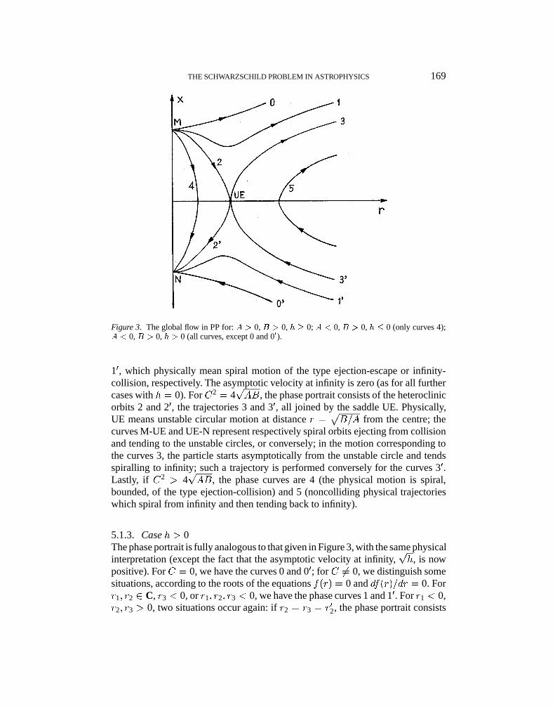
Figure 3. The global flow in PP for: A > 0, B > 0, h � 0; A < 0, B > 0, h � 0 (only curves 4);A < 0, B > 0, h > 0 (all curves, except 0 and 00).
10, which physically mean spiral motion of the type ejection-escape or infinity-collision, respectively. The asymptotic velocity at infinity is zero (as for all furthercases with h = 0). For C2 = 4
pAB, the phase portrait consists of the heteroclinic
orbits 2 and 20, the trajectories 3 and 30, all joined by the saddle UE. Physically,UE means unstable circular motion at distance r =
pB=A from the centre; the
curves M-UE and UE-N represent respectively spiral orbits ejecting from collisionand tending to the unstable circles, or conversely; in the motion corresponding tothe curves 3, the particle starts asymptotically from the unstable circle and tendsspiralling to infinity; such a trajectory is performed conversely for the curves 30.Lastly, if C2 > 4
pAB, the phase curves are 4 (the physical motion is spiral,
bounded, of the type ejection-collision) and 5 (noncolliding physical trajectorieswhich spiral from infinity and then tending back to infinity).
5.1.3. Case h > 0The phase portrait is fully analogous to that given in Figure 3, with the same physicalinterpretation (except the fact that the asymptotic velocity at infinity,
ph, is now
positive). For C = 0, we have the curves 0 and 00; for C 6= 0, we distinguish somesituations, according to the roots of the equations f(r) = 0 and df(r)=dr = 0. Forr1; r2 2 C, r3 < 0, or r1; r2; r3 < 0, we have the phase curves 1 and 10. For r1 < 0,r2; r3 > 0, two situations occur again: if r2 = r3 = r02, the phase portrait consists
as177.tex; 6/01/1998; 0:15; v.5; p.9

170 C. STOICA AND V. MIOC
of the separatrix f2; 20; 3; 30 UEg, where the distance of UE from the centre has thesame expression as in the case 5.1.1; if r2 < r02 < r3, the phase curves are 4 and 5.
5.2. THE CASE A < 0, B > 0
The phase portrait is quasi-identical to that given in Figure 3, with one exception:the curves 0 and 00 are no more present. In addition, the portret is valid for allvalues of h and C . The physical meaning of every phase curve has already beenspecified above for C 6= 0; for C = 0 there appear new interpretations.
5.2.1. Case h � 0Only the curves 4 form the phase portrait. When C = 0, they physically representrectilinear motion ejecting from collision, reaching a finite maximum distance,then coming back and ending in collision. It is to be noted that even for h = 0 theparticle cannot escape.
5.2.2. Case h > 0The situations mentioned for A > 0, B > 0, h > 0, governed by the roots of theequations f(r) = 0 and df(r)=dr = 0, repeat identically for C 6= 0. For C = 0we interpret them physically as follows: the curves 1 and 10 have respectively thesame significance as the curves 0 and 00 in Figures 2 or 3 (ejection-infinity orinfinity-collision rectilinear motion); UE represents unstable rest at distance rUEfrom the centre given by the same expression as in case 5.1.1; the curves 2 and 20
mean, respectively, radial motion ejecting from collision and tending to unstablerest, or conversely; as to the trajectories 3 and 30, they physically are rectilinearorbits starting from unstable rest and tending to infinity (with positive asymptoticvelocity), or conversely; finally, the curves 5 characterize radial motion comingfrom infinity, reaching a minimum distance, and then coming back to infinity. Thephysical interpretation of the curves 4 for C = 0 was already mentioned.
5.3. THE CASE A > 0, B < 0
The phase portrait (differentiated according to the values of h) is given in Figure 4,and is valid for every value of C .
5.3.1. Case h < 0If h � �4
3A2=C2, the real motion is impossible. For �4
3A2=C2 < h < 0, we
distinguish two main situations: if r1; r2 2 C, r3 < 0, the real motion is impossible,too; if r1 < 0, r2; r3 > 0, two cases can be separated. For r2 = r3 = r02, the phaseportrait reduces to the stable equilibrium SE (stable circular motion for C 6= 0,stable rest for C = 0); the expression of the distance rSE of SE from the centre isthe same as in case 5.1.1. For r2 < r02 < r3, the phase curves are 1. Their physicalinterpretation for C 6= 0 is already known (periodic or quasiperiodic trajectories);
as177.tex; 6/01/1998; 0:15; v.5; p.10

THE SCHWARZSCHILD PROBLEM IN ASTROPHYSICS 171
Figure 4. The global flow in PP for: A > 0, B < 0 (only SE and curves 1 for h < 0; only curves 2for h � 0); A < 0, B < 0 (only curves 2, and only for h > 0).
for C = 0 a new situation occurs: radial librations between a minimum (nonzero)and a maximum (finite) distance from the centre.
5.3.2. Case h � 0The phase portrait restricts to the curves 2, which physically represent spiral (forC 6= 0) or radial (for C = 0) noncolliding trajectories coming from infinity andthen tending back to infinity. Of course, the asymptotic velocity at infinity is zerofor h = 0 and positive for h > 0.
5.4. THE CASE A < 0, B < 0
5.4.1. Case h � 0In this case the real motion is impossible.
5.4.2. Case h > 0The phase portrait consists only of the curves 2 in Figure 4, and is valid for allvalues of C . The physical interpretation is fully analogous to that correspondingto the case A < 0, B > 0, h � 0 above; only the asymptotic velocity at infinity isalways positive.
as177.tex; 6/01/1998; 0:15; v.5; p.11
172 C. STOICA AND V. MIOC
6. Concluding Remarks
The present paper constitutes a first step towards the study of astrophysical prob-lems related to a potential of the form (1) by means of qualitative methods. Withinthis framework, we have considered the motion of a particle (dust, grain, or alarger body) in the photogravitational field of an oblate, rotating star (in the equa-torial plane of this one), or in a field whose gravitational component is featuredby Schwarzschild’s metric; both situations are very likely from the astrophysicalstandpoint.
Another goal of this study was to emphasize the usefulness of McGehee’stransformations in such problems. Using them, we blew up the collision singularityand obtained new, regularized equations of motion. This allowed the description ofthe (fictitious) flow on the collision manifold, necessary for the understanding ofnearby motion.
Following McGehee’s technique, the motion equations were restricted to anarbitrary energy level. To study the motion for all possible values of the energyconstant, we reduced the dimension of the phase space from 4 to 2 (using therotational symmetry of the global flow and the integral of angular momentum),then we analyzed the energy integral (20). This analysis allowed a full geometricand physical description of the possible motions.
Various families of trajectories were found, according to the interplay amongA, B, h, and C . Summarizing, the motion can be: bounded and collisional (of thetypes 0 ! rmax ! 0, 0 ! UE, UE ! 0); bounded and noncollisional (circular:SE and UE; noncircular: periodic – radial libration included – and quasiperiodic;the homoclinic orbit UE ! UE); unbounded and collisional (0 ! 1, 1 ! 0);unbounded and noncollisional (1! rmin !1,1!UE, UE!1). The richestcases in such possible situations are those tackled in Subsections 5.1.1–5.1.3 and5.2.3.
To end, some general features of the model are to be emphasized: the impos-sibility of escape for negative energy; the impossibility of collision for negativevalues ofB; the occurrence of the homoclinic loop in the case 5.1.1; the occurrenceof the black hole effect.
Acknowledgements
One of the authors (CS) was supported by the Romanian Ministry of Researchand Technology under contract 2097 GR/96. Useful discussions with Drs M.I.Piso, D. Selaru and F.N. Diacu are duly acknowledged. Thanks are also due to theanonymous referee for valuable comments and suggestions.
as177.tex; 6/01/1998; 0:15; v.5; p.12
THE SCHWARZSCHILD PROBLEM IN ASTROPHYSICS 173
References
Arnold, V.I.: 1974, Mathematical Methods in Classical Mechanics, Nauka, Moscow (Russian).Belenkii, I.M.: 1981, Celest. Mech. 23, 9.Blaga, P. and Mioc, V.: 1992, Europhys. Lett. 17, 275.Brumberg, V.A.: 1972, Relativistic Celestial Mechanics, Nauka, Moscow (Russian).Chandrasekhar, S.: 1983, The Mathematical Theory of Black Holes, Oxford University Press, Oxford.Cid, R., Ferrer, S. and Elipe, A.: 1983, Celest. Mech. 31, 73.Damour, T. and Schaefer, G.: 1986, Nuovo Cimento 101B, 127.Delgado, J., Diacu, F.N., Lacomba, E.A., Mingarelli, A., Mioc, V., Perez, E. and Stoica, C.: 1996, J.
Math. Phys. 37, 2748.Diacu, F.N., Mingarelli, A., Mioc, V. and Stoica, C.: 1995, in: R.P. Agarwal (ed.), Dynamical
Systems and Applications, World Scientific Series in Applicable Analysis, Vol. 4, World Scientific,Singapore, 213.
Eddington, A.S.: 1923, Mathematical Theory of Relativity, Cambridge University Press, Cambridge.McGehee, R.: 1974, Invent. Math. 27, 191.McGehee, R.: 1981, Comment. Math. Helvetici 56, 524.Saari, D.G.: 1974, Celest. Mech. 9, 55.Szebehely, V. and Bond, V.: 1983, Celest. Mech. 30, 59.
as177.tex; 6/01/1998; 0:15; v.5; p.13