The Einstein Field Equationson semi-Riemannian manifolds, and the Schwarzschild solution

Rasmus Leijon

VT 2012Examensarbete, 15hpKandidatexamen i tillämpad matematik, 180hpInstitutionen för matematik och matematisk statistik

Abstract

Semi-Riemannian manifolds is a subject popular in physics, with applicationsparticularly to modern gravitational theory and electrodynamics. Semi-Rieman-nian geometry is a branch of differential geometry, similar to Riemannian ge-ometry. In fact, Riemannian geometry is a special case of semi-Riemanniangeometry where the scalar product of nonzero vectors is only allowed to bepositive.

This essay approaches the subject from a mathematical perspective, provingsome of the main theorems of semi-Riemannian geometry such as the existenceand uniqueness of the covariant derivative of Levi-Civita connection, and someproperties of the curvature tensor.

Finally, this essay aims to deal with the physical applications of semi-Riemannian geometry. In it, two key theorems are proven - the equivalenceof the Einstein field equations, the foundation of modern gravitational physics,and the Schwarzschild solution to the Einstein field equations. Examples ofapplications of these theorems are presented.

Contents1 Introduction 4

2 Introduction to Semi-Riemannian Manifolds 82.1 Preliminaries . . . . . . . . . . . . . . . . . . . . . . . . . . . . . 82.2 Geometry . . . . . . . . . . . . . . . . . . . . . . . . . . . . . . . 92.3 Distance . . . . . . . . . . . . . . . . . . . . . . . . . . . . . . . . 182.4 Geodesics and parallel transport . . . . . . . . . . . . . . . . . . 192.5 Curvature . . . . . . . . . . . . . . . . . . . . . . . . . . . . . . . 22

3 Semi-Riemannian Geometry 283.1 Riemannian geometry . . . . . . . . . . . . . . . . . . . . . . . . 283.2 Lorentzian geometry . . . . . . . . . . . . . . . . . . . . . . . . . 293.3 Examples . . . . . . . . . . . . . . . . . . . . . . . . . . . . . . . 31

4 The Einstein Field Equations 344.1 Special relativity . . . . . . . . . . . . . . . . . . . . . . . . . . . 34

4.1.1 Generalization of Newtonian concepts . . . . . . . . . . . 354.2 General relativity . . . . . . . . . . . . . . . . . . . . . . . . . . . 36

4.2.1 The Einstein field equations . . . . . . . . . . . . . . . . . 374.3 The Schwarzschild geometry . . . . . . . . . . . . . . . . . . . . . 39

5 Applications to the Schwarzschild solution 505.1 The Schwarzschild manifold . . . . . . . . . . . . . . . . . . . . . 505.2 Schwarzschild geodesics . . . . . . . . . . . . . . . . . . . . . . . 505.3 Schwarzschild black holes . . . . . . . . . . . . . . . . . . . . . . 52

2

1 IntroductionIn 1905, Einstein published his annus mirabilis papers, among them the the-ory of special relativity ([1]). However, this theory had a flaw: incompatibilitywith gravitational fields. This led Einstein to consider the generalization of thistheory. In 1908, Minkowski examined the concept of spacetime from a mathe-matical perspective, introducing semi-Riemannian manifolds to assist with thephysical calculations ([10]). However, his original formulation of the differentialgeometry of these semi-Riemannian manifolds were not particularly mathemat-ical ([10]).

However, in terms of this semi-Riemannian geometry, Einstein formulatedhis theory of general relativity over the next decade, culminating in the Einsteinfield equations (see e.g. [2] and [3]). The general theory of relativity relates theenergy-momentum content of the physical universe to the curvature of the modelmanifold through these equations.

The first solution presented to the Einstein field equations was published byKarl Schwarzschild in 1916 ([19]), which has allowed us to make many physicalpredictions with increased precision. It is the unique solution for the field outsidea static, spherically symmetric body (see e.g. [4]). Even more impressively,Schwarzschild was actively serving as a lieutenant in the German artillery in thefirst World War while solving the Einstein field equations, dying from infectiononly some months after publishing his paper ([6]).

Examples of the improvements to physical theory includes the perihelionadvance of planets in our solar system, the deflection of light due to massiveobjects, the spectral shift of light due to massive objects and many more (see,e.g. [11] or [4]). From a physical perspective, this is very interesting. However,the Schwarzschild solution is not the only known solution to the Einstein fieldequations. Some of the famous solutions include the Kerr solution (for thespacetime surrounding a rotating mass), the Reissner-Nordström solution (forthe spacetime surrounding a charged mass) and the Kerr-Newman solution (forthe spacetime surrounding a charged and rotating mass) (see e.g. [5], chapter33 in [11] and [15]).

From a mathematical perspective, the theory of general relativity is inter-esting chiefly due to the semi-Riemannian geometry it is formulated in. Inthis essay, we will pursue a deeper understanding of these semi-Riemannianmanifolds and the geometries they result in. A semi-Riemannian manifold isa smooth manifold associated with a scalar product (a metric tensor) on itstangent bundle. This allows for mathematical generalizations of length, volumeand curvature. For this reason, the reader should be familiar with smooth man-ifolds and tensor algebra, as well as real analysis (see e.g. [21], [9] and [18] forbooks on these subjects).

In the theory of smooth manifolds, much effort is usually put into the smoothstructure of the manifold. In the theory of semi-Riemannian manifolds, focus isinstead directed at the geometry of the semi-Riemannian manifold. The readermay be familiar with Riemannian geometry, a branch of differential geometryintroduced by Bernhard Riemann in the middle of the 19th century ([17]). InRiemannian geometry, we study the geometry of smooth manifolds with an innerproduct (note the stronger requirement compared to the semi-Riemannian case)

4

on each tangent space of the manifold. Riemann’s formulation of Riemanniangeometry is a convenient generalization of the differential geometry of surfacesin Rn.

However, we are interested in the more general semi-Riemannian geometry,where the inner product on each tangent space of the manifold is replaced witha scalar product (no longer required to be positive definite). This may seema trivial generalization of Riemannian geometry, but the geometries of semi-Riemannian manifolds and Riemannian manifolds are in general completelydifferent. In semi-Riemannian geometry, we generalize many of the concepts wefind useful in the differential geometry on surfaces in Euclidean space such ascurvatures, straight lines and distances.

The main theorems, Theorems 4.4 (Theorem A) and 4.8 (Theorem B), ofthis paper are presented here, and the schematics of the proofs are given, giv-ing an implicit insight into the content and purpose of each chapter of this essay.

Theorem A: The Einstein TensorThe Einstein tensor, G = Ric − 1

2gS, is a symmetric, (0, 2) tensor field withvanishing divergence.

To construct the proof of this theorem, we need pieces taken from all parts ofthe foundation of semi-Riemannian geometry.

In chapter 2, we define the metric tensor g on the tangent bundle of a semi-Riemannian manifold (Definition 2.6). This tensor is a symmetric (0, 2) tensorfield.

In section 2.2, We then prove the uniqueness and existence of the covariantderivative (Theorem 2.17) on a semi-Riemannian manifold, which is a type ofconnection (see, e.g. chapters 12 and 13 in [7]). In section 2.5, we define interms of the covariant derivative the curvature tensor R (Definition 2.25). The(Riemann) curvature tensor R expresses the curvature of the semi-Riemannianmanifold. From this curvature tensor, we derive the Ricci tensor (Definition2.29), Ric, which is a contraction of the curvature tensor. Similarly, a contrac-tion of the Ricci tensor gives us the scalar curvature S (Definition 2.31). It isimportant for the proof of Theorem A that the Ricci tensor is symmetric, andwe prove this later in the section (Lemma 2.30).

Finally, we use the second Bianchi identity (also derived in chapter 2) toprove that div G = 0. Now it is clear what we need in order to prove TheoremA.

From the Einstein tensor, we define a set of nonlinear partial differential equa-tions solved for the geometry of the semi-Riemannian manifold M called theEinstein field equations, given by

Ric− 12gS = kT (1.1)

where T is the stress-energy tensor (Definition 4.2) which represents the energy-momentum content of the universe in the physical model. This is the main focusof this paper on semi-Riemannian manifolds and perhaps one of the main focusof the entire field of semi-Riemannian geometry.

5

Theorem B: The Schwarzschild SolutionLet (M,g) be a 4-dimensional Lorentzian manifold that is static, sphericallysymmetric and flat at infinity. Then in terms of the chart

(U , φ = (ct, R, θ, ϕ)

)the Einstein field equations (1.1) have a unique solution given by:

gαβ =

(1− rS

R

)0 0 0

0 −(1− rS

R

)−1 0 00 0 −R2 00 0 0 −R2 sin2 θ

where rS is a constant.

Theorem B is one solution to the Einstein field equations, defined earlier. How-ever, we will not only need an understanding of the Einstein field equations,but also a better understanding of the requirements on the semi-Riemannianmanifold. First, we shall clear up what we mean by a 4-dimensional Lorentzianmanifold. It is a semi-Riemannian manifold of metric signature (1, 3) (Defini-tions 3.2, 2.7 and 2.11, respectively).

Now, we will clearly also have to consider what we mean by sphericallysymmetric and static. We will find a definition of spherically symmetric inmore detail in e.g. Example 2.10 and section 3.3. A clearer definition will alsobe presented and justified in section 4.3. The term static is related to what wewill call causal characterization on Lorentzian manifolds. A deeper and detailedexplanation of causal characterization and Lorentzian manifolds will be givenin secion 3.2.

Finally, we will look at the Ricci tensor again to determine flatness at in-finity, because what we mean by flat is that the Ricci tensor vanishes. Now,solving these equations will take some work, however once topological and ge-ometrical properties of the manifold have been made rigorous, the problem ismainly calculus, and we shall solve it in great detail in section 4.3.

After these two theorems have been proven, we dedicate the final chapter, chap-ter 5, to geodesics (Definition 2.21) and black holes on the Schwarzschild mani-fold. Geodesics are, in short, the generalizations of straight lines to the curvedgeometry of semi-Riemannian manifolds, and as such are interesting mathemat-ically and physically, as we shall later see. Hence, chapter 5 gives two examples;geodesics of particles in orbit (crash- and bound orbits) around a massive objectas well as mathematical considerations of the Schwarzschild black hole.

Remark. From now on we will omit the word ‘smooth’ in this paper. It is thenconsidered implied that all functions, manifolds, structures, curves, and so on,are smooth, unless otherwise noted or inferred from context.

6

2 Introduction to Semi-Riema-nnian ManifoldsIn this chapter, we consider generalizations of geometrical concepts that weare at least intuitively familiar with in Euclidean space. We will talk aboutgeometry and metrics. In particular, the question we will ask ourselves is: howdo we measure lengths of curves and vectors?

This concept of metrics in geometry is not the same as the metric one wouldconsider in topology. In fact, most of the functions we will talk about in thischapter are not functions on a manifold itself, but on the tangent bundle orsections of the tangent bundle associated with a given manifold. We will dis-tinguish between the two when we feel it is important, but most of the time itis clear from context what we mean.

Furthermore, we will discuss curvature and parallel transport. Two moder-ately extensive examples are given in section 4.3, and the curious reader mayskip ahead.

It may be necessary to explain why we are starting with semi-Riemannianmanifolds instead of Riemannian manifolds, since semi-Riemannian manifoldsare in one sense an extension of Riemannian manifolds. From our perspective,however, Riemannian manifolds are simply a special case of semi-Riemannianmanifolds, and will be regarded as such throughout this paper, and Riemannianmanifolds will be explored in the section 4.1. Similarly, Lorentzian manifoldsare simply a special case of semi-Riemannian manifolds from our perspective,albeit the most interesting special case due to the practical applications of thesemanifolds. Therefore we will deal with them in the following chapters.

2.1 PreliminariesBefore we start discussing geometry, we have a few preliminary definitions totake care of. The reader should already be familiar with the topology of mani-folds, however we shall define some of the central mathematical objects that wewill be using. This is for added clarity, since the reader may be used to someother definition.

Definition 2.1 (Chart). An n-dimensional chart on a space M is a pair (U , φ)with U ⊂M, and with a coordinate map φ : U → φ(U) ⊆ Rn that is a bijectionfrom U onto some part of Rn.

We will talk about charts as coordinate systems on U , with coordinates φ =(u1, u2, ..., un). Similarly, we will think of atlases as a sort of collection of mu-tually overlapping charts on a manifold that allows us to construct a coordinatesystem for the manifold.

Definition 2.2 (Atlas). An n-dimensional atlas on a space M is a collection ofcharts (Uα, φα), that satisfies M =

⋃α Uα. For every pair of charts, (Uα, φα),

(Uβ , φβ), it is required that φα φ−1β and φβ φ−1

α are smooth functions.

We will at several points in this paper return to the topology of manifolds.Therefore we need to define the structure on a manifold.

8

Definition 2.3 (Structure). A structure on a set M is an equivalence class ofatlases: Aα : Aβ ∪ Aλ is an atlas for all β, α.

Definition 2.4 (Maximal atlas). A maximal atlas A is the union of all elementsin the structure, i.e. A =

⋃αAα.

Now we are ready to introduce the manifold.

Definition 2.5 (Manifold). An n-dimensional manifold is a set with a maximalatlas such that the topology induced by the maximal atlas is second countableand Hausdorff.

The maximal atlas through its associated charts provides a basis for a topologyon the manifold M, and it is this we mean by the topology being induced by themaximal atlas. Note also that the topology induced by the atlas A makes M atopological manifold. It is clear that this manifold is locally homeomorphic toRn. Finally, we are ready to focus on the geometry of manifolds.

2.2 GeometryThe metric tensor is what turns a manifold into a semi-Riemannian manifold,and allows for all the interesting and sometimes counter-intuitive properties andapplications of different semi-Riemannian manifolds that is the focus of effortswith these spaces. Again, note that this is not the same thing as a topologicalmetric (see e.g. chapters 7 and 8 in [18]).

Definition 2.6 (Metric tensor). Let M be a manifold and TM the tangentbundle of the manifold. The metric tensor, g, on M is a (0, 2) tensor field onTM, g : TM × TM → R, such that it assigns to each tangent space a scalarproduct, gp = 〈Xp, Yp〉.

This gp is required to vary smoothly over all points p ∈ M. The metrictensor is required to have the following properties for any two vector fields X,Y (or indeed vectors):

i. Symmetric: g(X,Y ) = g(Y,X),

ii. Nondegenerate: The set of functions fc : Y → g(Xc, Y ), for Xc a fixedvector field, is for all c not identically zero, provided Xc 6= 0.

It should be noted that this is not the definition of an inner product space. Aninner product gp is required to be positive definite, i.e. gp(X,Y ) > 0, X,Y 6= 0.However, this is not the case for this metric tensor, which is only required to benondegenerate (see e.g. chapter 3 in [16]).

Had we defined this metric tensor as an inner product space on each tan-gent space, we would have defined the metric tensor of a Riemannian manifold.Instead we keep this weaker definition and delve into the differences betweenRiemannian and semi-Riemannian further in chapter 4.

However, this is not the most general definition possible, and in fact there areapplications that make use of a nonsymmetric metric tensor - which of course isnot really a metric tensor of a semi-Riemannian manifold! This definition doesnot require g(X,Y ) = g(Y,X), which may seem very odd, but this definition

9

has its uses, for example in the nonsymmetric gravitational theory (see e.g.[12]).

Now we define our notation for the metric tensor. Keep in mind that it is atype of generalization of the inner product in Euclidean space, and is thereforeused to measure, for example, the length of vectors. However, note that it isnot required to be positive-definite, and therefore allows for semi-Riemannianmanifolds to be a type of manifold with very peculiar properties.

Let us introduce the coordinate basis of some coordinate system onM. Thenin terms of the chart

(U , φ = (u1, u2, ..., un)

), we denote the coordinate basis

by the set ∂1, ∂2, ..., ∂n, where of course we use the notation ∂α = ∂/∂uα.We denote the components of g relative to some coordinate basis by

gαβ = 〈∂α, ∂β〉,

and the n×n matrix of the components of g relative to an n-dimensional charton its semi-Riemannian manifold by [gαβ ]. Denote the inverse of this matrix byg−1, with components gαβ . This inverse must exist due to the nondegeneratenature of the metric tensor.

Let X, Y be two vector fields X =∑αX

α∂α and Y =∑α Y

α∂α. Here Xα

and Y α are the real-valued functions called the components of the vector fieldsX and Y . Since g is bilinear, g(X,Y ) can be written in terms of the productof its components:

g(X,Y ) = 〈X,Y 〉 =∑α

∑β

XαY β〈∂α, ∂β〉 =∑α

∑β

gαβXαY β .

Definition 2.7 (Semi-Riemannian manifold). AmanifoldM with an associatedmetric tensor g forms a pair (M,g). This pair is called a semi-Riemannianmanifold.

This has defined the most general space we will be looking at in this pa-per, namely the semi-Riemannian manifold. Usually we will denote a semi-Riemannian manifold with metric tensor g by M.

We are now interested in looking at some examples of semi-Riemannian man-ifolds. We will look at simple but useful examples. First, we study Euclideanspace, which the reader is probably intuitively familiar with (see e.g. chapter 1in [21] for a more thorough understanding).

Example 2.8 (Euclidean space). Let us denote the n-dimensional manifold ofEuclidean space by Rn, and its metric tensor by g. The cartesian coordinates(U , φ = (x1, x2, ..., xn)

)forms a structure for Rn by U = Rn, which means the

coordinates (U , φ) are global, which is rare in general. For this semi-Riemannianmanifold, the metric tensor is given by:

〈∂α, ∂β〉 = gαβ =

1 for all α = β,

0 otherwise.

Euclidean space is perhaps the most common space used, and therefore it isuseful to think of it as a special case of semi-Riemannian manifold. Since themetric tensor is positive definite, this is in fact also a Riemannian manifold.

10

Now we will look at a generalization of Euclidean space, which is calledsemi-Euclidean space (see e.g. chapter 3 in [16] for more detail). It is useful tounderstand the difference between Riemannian manifolds and semi-Riemannianmanifolds as somewhat analogous to the difference between Euclidean space andsemi-Euclidean space.Example 2.9 (Semi-Euclidean space). Let us denote the (n + ν)-dimensionalmanifold of semi-Euclidean space by Rnν , and its metric tensor by g. In termsof the cartesian coordinates

(U , φ = (x1, x2, ..., xn)

), the structure of Rnν is the

same as for the Euclidean space R(n+ν), which means that(U , φ = (x1, x2, ..., xn)

)is a global coordinate system. For Rnν , the metric tensor is given by:

〈∂α, ∂β〉 = gαβ =

1 for all α = β ≤ ν,−1 for all α = β > ν,

0 otherwise.

We shall think of semi-Euclidean space as a model space for a semi-Riemannianmanifold. Notice that clearly in this metric, the scalar product of two vectorscan be negative.

As a last example of a semi-Riemannian manifold, we take the 2-sphere S2

(for more detail, see e.g. chapter 5 in [21]).Example 2.10 (2-Sphere). Let us define S2 as the sphere of unit radius withassociated metric tensor g. Using the cartesian coordinates of Euclidean R3,defined globally, we set S2 as all the points satisfying (x1)2 + (x2)2 + (x3)2 = 1.

Typically, we find an atlas on S2 by dividing the sphere into six hemispheres(six charts):

U1 = (x1, x2, x3) : x1 > 0, φ = (x2, x3),U2 = (x1, x2, x3) : x1 < 0, φ = (x2, x3),U3 = (x1, x2, x3) : x2 > 0, φ = (x1, x3),U4 = (x1, x2, x3) : x2 < 0, φ = (x1, x3),U5 = (x1, x2, x3) : x3 > 0, φ = (x1, x2),U6 = (x1, x2, x3) : x3 < 0, φ = (x1, x2).

On each one, only two coordinates are needed to describe each point. Expressedin what we will call spherical coordinates, (U , φ = (θ, ϕ)). This gives us themetric tensor components

〈∂α, ∂β〉 = gαβ =[1 00 sin2 θ

]Now we have a good idea of the structure of the 2-sphere, as well as its geometry.It is a type of Riemannian manifold as we will see in the next chapter. This2-sphere will be examplified in section 3.3, since we will use it in the applicationsto gravitational theory.

We will need to define a few more properties of the metric on a semi-Riemannian manifold. Clearly, we will need a way to categorize semi-Riemannianmanifolds to distinguish between manifolds with different properties. We usewhat is called the metric signature to do this. (see e.g. chapter 1 in [9]).

11

Definition 2.11 (Metric signature). The signature of a metric tensor g is thenumber of positive (m) and negative (n) eigenvalues of the matrix [gαβ ], usuallydenoted as a pair, (m,n), m,n ∈ N. The manifold M of the metric tensor g issaid to be of dimension m+ n, and is said to have the metric signature (m,n)

Now we introduce a brief example so that the significance of this classifica-tion is more obvious to the reader. We shall show the metric signature of theMinkowski space, which is a semi-Riemannian manifold named after the 19thcentury mathematician Hermann Minkowski ([10]).

Example 2.12 (Metric signature of a Minkowski space). Let M be a semi-Euclidean space with n = 1 and ν = 3, i.e. M = R1

3. Then we call Mthe Minkowski space. Then it has a metric tensor that is usually called η.For cartesian coordinates, the chart

(U , φ = (x1, x2, x3, x4)

), where once again

U = R(n+ν) is global. Then the components of η are given by

〈∂α, ∂β〉 = ηαβ =

1 0 0 00 −1 0 00 0 −1 00 0 0 −1

The metric tensor clearly has one positive eigenvalue and three negative eigen-values and therefore a metric signature of (1, 3).

The Minkowski space is a semi-Riemannian manifold that is used particu-larly in the special theory of relativity. We will talk about it in a little moredetail in section 4.1.

Furthermore, we will need to introduce a useful tool when dealing with distanceson a manifold. This is called the line element, and it can be thought of asdescribing an infinitesimal distance on a manifold.

Definition 2.13 (Line element on a manifold). Let M be a semi-Riemannianmanifold with associated metric tensor g. Then, in terms of a coordinate chart(U , φ = (u1, u2, ..., un)), the line element q is defined as a quadratic form of gp,such that q(X) = 〈X,X〉. Since

q(X) =∑α

∑β

gαβXαXβ =

∑α

∑β

gαβduα(X)duβ(X),

we write q as the product

q =∑α

∑β

gαβduαduβ ,

This definition is used for example in chapter 3 in [16].

From these definitions, particularly the definition of a metric tensor, we canfind new properties of the tangent bundles of our manifolds. Remembering that[X,Y ] is the Lie bracket of vector fields, we can define the covariant derivative,which is a connection on the tangent bundle (see, e.g. chapter 5 in [7] for thedefinition of Lie bracket).

12

Definition 2.14 (Covariant derivative). LetM be a semi-Riemannian manifoldwith tangent bundle TM. Let X and Y be vector fields in the tangent bundle.

Then we define the covariant derivative relative to X, ∇X , as a function∇XY : X(U)× X(U)→ X(U) with the following properties:

i. The covariant derivative of a real-valued function coincides with the direc-tional derivative of the function: ∇Xf = Xf ,

ii. It is linear in the first variable and additive in the second variable:

∇fX+gY (Z +W ) = f∇XZ + g∇Y Z + f∇XW + g∇YW,

iii. It is Leibnizian in the second variable:

∇XfY = f∇XY + Y∇Xf = f∇XY + Y Xf,

iv. It is torsion-free: ∇XY −∇YX = [X,Y ],

v. It is compatible with the metric: X〈Y, Z〉 = 〈∇XY, Z〉+ 〈Y,∇XZ〉,

for X,Y, Z,W ∈ X(U) and f, g ∈ C∞(U).

This definition of the covariant derivative is often called the Levi-Civita con-nection, and is a special type of connection. Many other authors make use ofthe more general object of connections, usually defined as a function with theproperties i) through iii) (see, e.g. chapter 3 in [16] or chapter 12 in [7]).

Since we do not take interest in any connection other than the covariantderivative, this definition is sufficient.

This definition of the covariant derivative will lead to a special type of func-tion, namely the covariant derivative of a coordinate vector relative to anothercoordinate vector. Even though this may seem like an innocuous enough func-tion, we will soon see that it is useful in describing curves on a manifold.

Since we can write a vector field X in terms of the coordinate basis asX =

∑αX

α∂α, with Xα ∈ C∞(M), we must surely be able to do the samething with the covariant derivative (see e.g. chapter 4 in [7]).

Definition 2.15 (Christoffel symbols). A chart (U , φ) on a semi-Riemannianmanifold M has a set of Christoffel symbols, functions Γλαβ : U → R defined by:

∇∂α∂β =∑λ

Γλαβ∂λ.

Lemma 2.16 (The Koszul formula). Let M be a semi-Riemannian manifoldwith associated metric tensor g. Then the covariant derivative satisfies theKoszul formula:

2〈∇XY,Z〉 = X〈Y, Z〉+ Y 〈Z,X〉 − Z〈X,Y 〉− 〈Y, [X,Z]〉 − 〈Z, [Y,X]〉 − 〈X, [Z, Y ]〉. (2.1)

Proof. Inspired by the proof Theorem 11 in [16], according to property v) of thecovariant derivative it is metric compatible, i.e.

X〈Y,Z〉 = 〈∇XY,Z〉+ 〈Y,∇XZ〉.

13

Cyclically permuting this equation, we get two more equations,

Y 〈Z,X〉 = 〈∇Y Z,X〉+ 〈Z,∇YX〉,

Z〈X,Y 〉 = 〈∇ZX,Y 〉+ 〈X,∇ZY 〉.

Now, from the torsion-free property of the covariant derivative, we rewrite thelast term of each equation as ∇XY = [X,Y ]+∇YX. These three equations arethen given by

X〈Y, Z〉 = 〈∇XY, Z〉+ 〈Y,∇ZX〉+ 〈Y, [X,Z]〉, (2.2a)

Y 〈Z,X〉 = 〈∇Y Z,X〉+ 〈Z,∇XY 〉+ 〈Z, [Y,X]〉, (2.2b)

Z〈X,Y 〉 = 〈∇ZX,Y 〉+ 〈X,∇Y Z〉+ 〈X, [Z, Y ]〉. (2.2c)

Remembering that the metric tensor is symmetric, we can simplify the right-hand side of (2.2a) + (2.2b) − (2.2c), giving us:

X〈Y, Z〉+ Y 〈Z,X〉 − Z〈X,Y 〉= 2〈∇XY,Z〉+ 〈Y, [X,Z]〉+ 〈Z, [Y,X]〉+ 〈X, [Z, Y ]〉,

which becomes:

2〈∇XY,Z〉 = X〈Y, Z〉+ Y 〈Z,X〉 − Z〈X,Y 〉− 〈Y, [X,Z]〉 − 〈Z, [Y,X]〉 − 〈X, [Z, Y ]〉.

This is called the Koszul formula and it is a useful property as we shall see inthe proof of Theorem 2.17.

After this technical lemma, we are ready to prove the main theorem of thissection.

Theorem 2.17 (Existence and uniqueness of the covariant derivative). Let Mbe a semi-Riemannian manifold with associated metric tensor g. Then thereexists a unique covariant derivative on M.

Proof. Inspired by the proof of Theorem 11 in [16], we prove this theorem. Firstwe prove the uniqueness of the covariant derivative: If the covariant derivativeis not unique, then there exists another covariant derivative, say ∇′. However,note that the right-hand side of the Koszul formula (2.1) does not depend onthe covariant derivative.

Therefore, we use the Koszul formula for the two operators ∇ and ∇′. Thisgives us

2〈∇′XY,Z〉 − 2〈∇XY,Z〉 = 0,

and

〈(∇′X −∇X)Y,Z〉 = 0,

and obviously this proves that ∇′ = ∇.

14

Now we prove the existence of the covariant derivative: Since any vector canbe written in terms of a coordinate basis, we may without loss of generality usethe coordinate basis of some chart, (U , φ). We then know that [∂α, ∂β ] = 0 forall α, β.

Because of this, we can rewrite the Koszul formula (2.1) in terms of thecoordinate basis

2〈∇∂α∂β , ∂λ〉 = ∂α〈∂β , ∂λ〉+ ∂β〈∂λ, ∂α〉 − ∂λ〈∂α, ∂β〉. (2.3)

From the definition of the Christoffel symbols (2.15), and the definition of themetric tensor components, we can write equation (2.3) as∑

µ

Γµαβgµλ = 12 (∂αgβλ + ∂βgλα − ∂λgαβ) . (2.4)

Multiplying by the metric tensor inverse, gλν and summing over λ we finallyarrive at,

Γναβ = 12∑λ

gλν (∂αgβλ + ∂βgλα − ∂λgαβ) , (2.5)

due to the property∑α gαβg

αλ = δλβ , where δλβ is the Kronecker delta function.This clearly defines a covariant derivative on any chart (U , φ), since it fulfills

all conditions for a covariant derivative.

First we prove that property i) holds: This property follows from the proof ofproperty iii), which we will soon get to.

Now we prove that property ii) holds: We use the Koszul formula (2.1) as thebasis for this proof. First we prove linearity in the first variable. As we explainedpreviously, we can without loss of generality use f∂α + h∂β as X, ∂λ as Y and∂ν as Z in the Koszul formula. This gives us:

2〈∇f∂α+h∂β∂λ, ∂ν〉 = (f∂α + h∂β)〈∂λ, ∂ν〉+ ∂λ〈∂ν , (f∂α + h∂β)〉−∂ν〈(f∂α + h∂β), ∂λ〉 − 〈∂λ, [(f∂α + h∂β), ∂ν ]〉 (2.6)

−〈∂ν , [∂λ, (f∂α + h∂β)]〉 − 〈(f∂α + h∂β), [∂ν , ∂λ]〉.

What we will prove is therefore that the right-hand side of (2.6) is equal to

2f∑ρ

Γραλgρν + 2h∑ρ

Γρβλgρν .

This is proven by rewriting the right-hand side of equation (2.6), and usingthe linearity property of the metric tensor, and by [∂ν , ∂λ] = 0 for all ν, λ, thisbecomes

f∂α〈∂λ, ∂ν〉+ h∂β〈∂λ, ∂ν〉+ ∂λ (f〈∂ν , ∂α〉) + ∂λ (h〈∂ν , ∂β〉)− ∂ν (f〈∂α, ∂λ〉)− ∂ν (h〈∂β , ∂λ〉)− 〈∂λ, [(f∂α + h∂β), ∂ν ]〉 − 〈∂ν , [∂λ, (f∂α + h∂β)]〉.

15

By the definition of the Lie bracket and the linearity property of the metrictensor, this can be rewritten

f∂αgλν + h∂βgλν + f∂λgνα + h∂λgνβ − f∂νgαλ − h∂νgβλ−〈∂λ, ((f∂α+h∂β)∂ν−∂ν(f∂α+h∂β))〉−〈∂ν , (∂λ(f∂α+h∂β)−(f∂α+h∂β)∂λ)〉,

and

f∂αgλν + h∂βgλν + f∂λgνα + ∂λfgνα + h∂λgνβ + ∂λhgνβ − f∂νgαλ− ∂νfgαλ − h∂νgβλ − ∂νhgβλ + ∂νfgλα + ∂νhgλβ − ∂λfgνα − ∂λhgνβ .

Half of these terms cancel each other out, leaving:

f∂αgλν + h∂βgλν + f∂λgνα + h∂λgνβ + ∂λhgνβ − f∂νgαλ − h∂νgβλ= 2f

∑ρ

Γραλgρν + 2h∑ρ

Γρβλgρν .

Now, we return to the Koszul formula to prove linearity in the second variable.We recall that we can without loss of generality use ∂α instead of X, ∂β + ∂λinstead of Y and ∂ν instead of Z. Then, equation (2.1) becomes

2〈∇∂α(∂β+∂λ), ∂ν〉 = ∂α〈(∂β+∂λ), ∂ν〉+(∂β+∂λ)〈∂ν , ∂α〉−∂ν〈∂α, (∂β+∂λ)〉− 〈(∂β + ∂λ), [∂α, ∂ν ]〉 − 〈∂ν , [(∂β + ∂λ), ∂α]〉 − 〈∂α, [∂ν , (∂β + ∂λ)]〉. (2.7)

Now we prove that the right-hand side of this equation is equal to 2∑µ Γµαβgµν+

2∑µ Γµαλgµν . Clearly the last three terms of the right-hand side of equation

(2.7) are zero. By linearity of the metric tensor, the right-hand side of (2.7)becomes

∂αgβν + ∂αgλν + ∂βgνα + ∂λgνα − ∂νgαβ − ∂νgαλ= 2

∑µ

Γµαβgµν + 2∑µ

Γµαλgµν .

Therefore, property ii) is satisfied.

Now we prove that property iii) holds: Again using the Koszul equation (2.1),and again we remember that we can use ∂α instead of X, f∂β instead of Y and∂λ instead of Z. Using this, we arrive at

2〈∇∂αf∂β , ∂λ〉 = ∂α〈f∂β , ∂λ〉+ f∂β〈∂λ, ∂α〉 − ∂λ〈∂α, f∂β〉− 〈f∂β , [∂α, ∂λ]〉 − 〈∂λ, [f∂β , ∂α]〉 − 〈∂α, [∂λ, f∂β ]〉.

We note that what we actually want to prove is that the right-hand side is equalto 2(∂αfgβλ + f

∑µ Γµαβgµλ). Then we can rewrite the right-hand side of this

equation.We expand the last three terms by the definition of the Lie bracket, and by

the linearity property of the metric tensor we find it to be equal to

∂α(fgβλ) + f∂βgλα − ∂λ(fgαβ)− 〈∂λ, (f∂α − ∂αf)∂β〉 − 〈∂α, (f∂λ − ∂λf)∂β〉.

16

Recognizing that only one term in each Lie derivative remains nonzero, by thesymmetry and linearity properties of the metric tensor, this equation is equalto

∂αfgβλ + f∂αgβλ + f∂βgλα − ∂λfgαβ − f∂λgαβ + ∂αfgλβ + ∂λfgαβ

finally, some terms cancel, leaving

2∂αfgβλ + f∂αgβλ + f∂βgλα − f∂λgαβ = 2(∂αfgβλ + f∑µ

Γµαβgµλ).

This clearly proves that the covariant derivative is Leibnizian in the secondvariable.Now we prove that property iv) holds: Since [∂α, ∂β ] = 0 for all α, β, this prop-erty simply gives us Γναβ = Γνβα in terms of the metric tensor.

Now we prove that property v) holds: It is no loss of generality to prove that∂α〈∂β , ∂λ〉 = 〈∇∂α∂β , ∂λ〉+ 〈∂β ,∇∂α∂λ〉 or in terms of Γ and the metric tensorcomponents:

∂αgβλ =∑µ

Γµαβgµλ +∑µ

Γµαλgµβ .

The right-hand side can be written, using equation (2.4) and the symmetry ofthe metric tensor, as∑

µ

Γµαβgµλ +∑µ

Γµαλgµβ = 12 (∂αgβλ + ∂βgλα − ∂λgαβ)

+12 (∂αgλβ + ∂λgβα − ∂βgαλ) = ∂αgβλ.

Thus, we have proven that the covariant derivative exists on every chart of amanifold M, and that it is unique.

Corollary 2.18 (Christoffel symbols in terms of the metric tensor). On somechart (U , φ = (u1, u2, ..., un)) of a semi-Riemannian manifold M, the Christoffelsymbols are given in terms of the metric tensor components by:

Γναβ = 12∑λ

gλν (∂αgβλ + ∂βgλα − ∂λgαβ) . (2.8)

Proof. This follows from the proof of Theorem 2.17, see equation (2.5).

As a last part of derivatives on semi-Riemannian manifolds, we will gener-alize the concept of the divergence to apply to tensors on a semi-Riemannianmanifold. This is defined in terms of the covariant derivative, and is thereforerelated to normal divergence as the normal derivative is related to the covariantderivative (see e.g. chapter 7 in [9]).

Definition 2.19 (Divergence). Let M be a semi-Riemannian manifold withcovariant derivative ∇. Then the divergence of a tensor τ is defined as thecontraction

divβ τ = Cβα(∇∂ατ ). (2.9)

17

Expressed in components of the (r, s) tensor τ , this becomes

divαnτα1,...,αn,...,αrβ1,...,βs

=∑αn

∇∂αn τα1,...,αn,...,αrβ1,...,βs

. (2.10)

For symmetric (0, 2) and (2, 0) tensors τ , we skip the subscript for the di-vergence, since it does not matter which divergence we take, and write thedivergence of τ as div τ .

In this paper we will mainly be interested in div τ = 0, due to the physicalsignificance. We are chiefly interested in the case when the energy and momen-tum content of the universe has zero divergence, that is, when there is no energyor momentum disappearing from the universe.

2.3 DistanceWe will talk a lot about distances, lengths of vectors and similar. Some authorsdislike using the word length since a null curve has length zero by this definition.However, stretching the normal concept of length, we may as well call this Lthe length of a curve on a semi-Riemannian manifold.

It may be useful for most readers at this point to note that the word metricthat we use regularly in this paper is not a metric in the topological sense.When we talk about the geometry of a manifold, it is the properties of the innerproduct on its tangent bundle we mean. This in turn gives a new meaning tointegral curves on the manifold, the differential geometry of the manifold. Itis in this sense that we use the words geometry and metric. In fact, at severalpoints we will use the term ‘on the manifold’ when we in fact mean on thetangent bundle of the manifold, or perhaps even only in some local tangentspace. This should not cause any confusion, and in fact what we really meanshould be clear from context.

The concept of length holds up in positive-definite (metric signature withn = 0) geometry, where all nonzero vectors have nonzero length, as well asindefinite (n 6= 0) geometry, where a vector may well have negative length insome sense, although of course the arc length of a curve cannot be negative.

Definition 2.20 (Arc length). Let M be some semi-Riemannian manifold, andlet γ : I → M be a curve on some chart (U , φ). Then we define the arc lengthof the curve γ as:

L =∫I

|γ(s)|ds =∫I

|〈γ(s), γ(s)〉|1/2ds,

which with our notation for the metric tensor, this can be rewritten:

L =∫I

∣∣∣∣∣∣∑αβ

gαβduα γ(s)

ds

duβ γ(s)ds

∣∣∣∣∣∣1/2

ds.

This arc length of a curve is unchanged by monotone reparametrization (see,e.g. chapter 5 in [16]).

Since we now have the concepts of both lengths of curves and length ofvectors on a semi-Riemannian manifold M, we have the tools necessary to talk

18

about minimizing the arc length L between two points on M. In normal Eu-clidean space, the shortest distance between two points is a straight line.

We will generalize this concept of a straight line in an intuitive fashion,and so we will be able to visualize even high-dimensional, general manifolds asanalogous to a curved Euclidean space.

2.4 Geodesics and parallel transportOn some semi-Riemannian manifold M, the concept of a shortest path orstraight line can be generalized. It can be thought of as a curve γ, whosevector field γ is parallel. This concept of a straight line, or geodesic, is widelyused in physical applications.

Let the tangent vector field along the curve γ be denoted by γ. This γis therefore the directional derivative. Let us parametrize the curve using anaffine parameter s, so that, using this coordinate, γ = γ(s). Then the directionalderivative, the vector field γ, is the derivative, dγ/ds. For γ to be parallel, wewill require that ∇γ γ = 0.

Definition 2.21 (Geodesic). Let M be a semi-Riemannian manifold and letγ : [p, q]→M be a curve on M. Then γ is a geodesic if ∇γ γ = 0.

We shall now formulate the differential equations that describe these geodesics,and further we will prove the uniqueness and existence of geodesics.

Theorem 2.22 (Existence and uniqueness of geodesic equations). Let M be asemi-Riemannian manifold and let γ : [p, q] → M be a curve on M. If γ is ageodesic the coordinate functions uαγ on some chart (U , φ) satisfy the geodesicequations:

d2(uλ γ(s))ds2 +

∑α

∑β

Γλαβd(uα γ(s))

ds

d(uβ γ(s))ds

= 0. (2.11)

For each geodesic, these equations have unique solutions.

Proof. First, we will prove the equivalence between the definition of a geodesic,that is ∇γ γ = 0, and the geodesic equations. Then we will argue for the unique-ness and existence of the solutions to the geodesic equations.

First, we prove equivalence: For a curve γ, the vector field along the curve, γ,can be rewritten

γ =∑α

γα∂α.

Using this with the definition of a geodesic gives us from the Leibnizian propertyof the covariant derivative:

∇γ γ = ∇γ∑α

γα∂α =∑α

(∇γ γα)∂α +∑α

γα(∇γ∂α).

Now, for the first sum, it is clear that the covariant derivative relative to thevector curve γ is simply the derivative of the vector field on the curve relativeto the parameter s, i.e. ∇γ γα = γα.

19

Using this along with the linearity property of∇γ = ∇Σβ γβ∂β , we can rewritethis equation as

∇γ γ =∑α

γα∂α +∑α

γα(∇Σβ γβ∂β∂α),

and using property ii) of the definition of the covariant derivative, this equationbecomes

∇γ γ =∑α

γα∂α +∑α

∑β

γαγβ(∇∂β∂α).

Now, using Definition 2.21 on the left-hand side of this equation, and Definition2.15, we obtain

0 =∑α

γα∂α +∑α

∑β

γαγβ∑λ

Γλβα∂λ.

and if we change the index in the first term from α to λ, we get

0 =∑λ

γλ +∑α

∑β

γαγβΓλβα

∂λ.

Clearly equivalence is only held in general if each term of this sum over λ iszero, when the components of this vector are all zero. That is,

γλ +∑α,β

γαγβΓλβα = 0.

Since γα = uα γ, these are the geodesic equations and we have derived ourgeodesic equations from the definition of the geodesic.

Proving existence and uniqueness of the solutions: To prove uniqueness andexistence, we need only note that putting y = γ, we get the system of first-order equations

yλ = γλ,

yλ = −∑α

∑β y

αyβΓλβα,

and by the existence and uniqueness theorem for first-order ordinary differentialequations, there exists a unique solution for this system of equations, for everygiven set of initial conditions γ(s0) = p, γ(s0) = Xp imposed upon it (see, e.g.Theorem 4.1 in [20]).

This next example is an immediate application of equation (2.11). In it,we study the geodesic equations for an orthogonal coordinate system, or moreaccurately, an orthogonal coordinate basis.

Expressed in terms of the metric tensor components, orthogonality requiresthat gαβ = 0 for α 6= β. This leads to the geodesic equations, which are normallyquite complicated, to take a much simpler form.

20

Example 2.23 (Geodesic equations in orthogonal coordinates). In this exam-ple, inspired by Exercise 3.15 in [16], we will examine the geodesic equationsin orthogonal coordinates closely. Orthogonal coordinates are in practice verycommon, for example the Schwarzschild solution to the Einstein field equationsis orthogonal (see (5.2)). Similarly, both examples in section 4.3 are orthogonal.

Let M be a semi-Riemannian manifold with metric tensor g. For a chart(U , φ), the coordinate basis is said to be orthogonal if the metric tensor relativeto φ has the property gαβ = 0 if α 6= β.

Notice that this makes the sum in the definition of the Christoffel symbolsfrom (2.8), vanish. Equation (2.8) then becomes

Γλαβ = 12g

λλ(∂αgβλ + ∂βgλα − ∂λgαβ)

This allows us to make the general geodesic equations, equation (2.11), a littlemore manageable as

d2uλ γ(s)ds2 + 1

2∑α

∑α

gλλ∂αgβλduα γ(s)

ds

duβ γ(s)ds

+ 12∑α

∑β

gλλ∂βgλαduα γ(s)

ds

duβ γ(s)ds

− 12∑α

∑β

gλλ∂λgαβduα γ(s)

ds

duβ γ(s)ds

= 0.

From the assumption of orthogonality, we have that in the second term, β = λis the only nonzero case, in the third only α = λ is nonzero and in the fourth,only α = β is nonzero.

Replacing the index α for β in the third term, we see that the second termand third term are equal and we can rewrite these equations as

d2uλ γ(s)ds2 + gλλ

∑α

∂αgβλduα γ(s)

ds

duλ γ(s)ds

− 12g

λλ∑α

∂λgααduα γ(s)

ds

duα γ(s)ds

= 0.

Lastly, we multiply by gλλ and by some straightforward calculations we obtainthe geodesic equations for orthogonal coordinates

d

ds

(gλλ

duλ

ds

)− 1

2∑α

∂λgαα

(duα

ds

)2= 0. (2.12)

These equations are much simpler to use and therefore very practical for allpractical cases we will consider in this paper. In fact, all metric tensors presentedin this paper are orthogonal, and therefore this version of the geodesic equationshold on all manifolds considered.

Next, we present a proposition for geodesic parametrization. We will not needto use the results explicitly, but it will provide insight in how we are allowed toparametrize geodesics.

21

This will be particularly useful for the reader in the following chapters,where we will consider geodesics parametrized by what is called proper time(see e.g. chapter 3 and 4 in [4] for more details on the physical significance ofthis proposition).

Proposition 2.24 (Geodesic parametrization). Let γ : I →M be a nonconstantgeodesic on some semi-Riemannian manifold M. A reparametrization γ of γusing a function f : I → J is a geodesic if f(s) = as+ b, a, b ∈ R.

Proof. If γ = γ(s) is a geodesic and f is some real-valued function, then thereparamatrized curve γ = γ f needs to satisfy the geodesic equations, and∇γ γ = 0 becomes, writing dγ/ds as ˙γ:

∇ ˙γ ˙γ = ∇ ˙γ

(dγ

df

df

ds

)= df

ds

(∇ ˙γ

dγ

df

)+ dγ

df

(∇ ˙γ

df

ds

).

Since obviously ∇ ˙γ(dγ/df) = 0, it is required that ∇ ˙γ(df/ds) = d2f/ds2 = 0,and that requires from the function f that f = as+ b.

2.5 CurvatureNow, having defined the length of a curve and a geodesic, we can further un-derstand a semi-Riemannian manifold if we think of the geometry as defined byhow we measure distance between points. However, there is another useful toolwhen we consider the geometry of a manifold, and that is the curvature of themanifold.

So what is the purpose of the curvature tensor? Well, visualizing the paralleltransport of a vector around a closed curve γ, one would expect the change inthe vector to be zero, and in Euclidean space this is true. However, this is nottrue in general, and generally one may expect a difference which depends on thecurvature. Therefore, we can think of the curvature as somewhat analogous tothe difference between the start vector and end vector when parallel transportedin a closed loop on the manifold.

In fact, we may define flatness at a point p of a semi-Riemannian manifoldM by every component of the curvature tensor being equal to zero at that point(see e.g. chapter 13 in [7] for more details).

Definition 2.25 (Curvature tensor). The curvature tensor (sometimes calledthe Riemann curvature tensor), is a (1, 3) tensor field, R : X(M)3 → X(M) suchthat

RXY Z = ∇[X,Y ]Z − [∇X ,∇Y ]Z,

where X,Y, Z ∈ X(M).

Proposition 2.26 (Curvature tensor properties). The curvature tensor R hasthe following properties

i. Skew-symmetry: RXY = −RY X ,

ii. First Bianchi identity: RXY Z + RY ZX + RZXY = 0,

iii. Metric skew-symmetry: 〈RXY Z,W 〉 = −〈RXYW,Z〉.

22

for all X,Y, Z,W ∈ X(M)

Proof. Proving property i): The property i) is obvious since the Lie bracket isskew-symmetric, and thus from the definition of the curvature tensor and thecovariant derivative, with very simple algebra this property follows.

Proving property ii): The second property is perhaps not so obvious, but rewrit-ing the left side of this equality by the definition of the curvature tensor as

RXY Z + RY ZX + RZXY = ∇[X,Y ]Z − (∇X∇Y −∇Y∇X)Z+∇[Y,Z]X − (∇Y∇Z −∇Z∇Y )X +∇[Z,X]Y − (∇Z∇X −∇X∇Z)Y

= ∇[X,Y ]Z +∇[Y,Z]X +∇[Z,X]Y −∇X(∇Y Z −∇ZY )−∇Y (∇ZX −∇YX)Z −∇Z(∇XY −∇YX).

From the torsion-free property of the covariant derivative and the definition ofthe Lie bracket we get that

∇[X,Y ]Z +∇[Y,Z]X +∇[Z,X]Y −∇X [Y,Z]−∇Y [Z,X]−∇Z [X,Y ]= [[X,Y ], Z] + [[Y,Z], X] + [[Z,X], Y ] = 0,

by the Jacobi identity (see e.g. page 92 in [7]).

Proving property iii): Now, it is sufficient to prove that

〈RXY Λ,Λ〉 = 0 for all Λ,

since then, for Λ = X + Y ,

〈RXYX+Y,X+Y 〉 = 〈RXYX,X〉+〈RXY Y, Y 〉+〈RXYX,Y 〉+〈RXY Y,X〉= 〈RXYX,Y 〉+ 〈RXY Y,X〉 = 0.

From the definition of the curvature tensor and the linearity of the metric tensorwe have that

〈RXY Λ,Λ〉 = 〈∇[X,Y ]Λ,Λ〉 − 〈∇X∇Y Λ,Λ〉+ 〈∇Y∇XΛ,Λ〉,

and from the metric compatibility property of Definition 2.14, we get for eachterm of the right hand side of this equation

〈∇[X,Y ]Λ,Λ〉 = [X,Y ]〈Λ,Λ〉/2,

〈∇X∇Y Λ,Λ〉 = X〈∇Y Λ,Λ〉 − 〈∇XΛ,∇Y Λ〉 = XY 〈Λ,Λ〉/2− 〈∇XΛ,∇Y Λ〉,

〈∇Y∇XΛ,Λ〉 = Y 〈∇XΛ,Λ〉 − 〈∇Y Λ,∇XΛ〉 = Y X〈Λ,Λ〉/2− 〈∇XΛ,∇Y Λ〉.

Hence,

〈RXY Λ,Λ〉 = [X,Y ]〈Λ,Λ〉/2−XY 〈Λ,Λ〉/2 + Y X〈Λ,Λ〉/2 = 0,

Thus, 〈RXY Λ,Λ〉 = 0.

Mostly in calculations, we are interested in differential equations of real-valued functions. Therefore we are interested in the real-valued components ofthe curvature tensor, which we will use in later chapters and examples.

23

Theorem 2.27 (Curvature tensor components). For some chart (U , φ) on asemi-Riemannian manifold M, the components of R relative to the coordinatesystem are given by

R∂α∂β∂λ =∑µ

Rµλαβ∂µ, (2.13)

where the real-valued functions Rµλβα are given by

Rµλβα = ∂αΓµβλ − ∂βΓµαλ +∑ν

ΓµανΓνβλ −∑ν

ΓµβνΓναλ.

Proof. In terms of coordinate vector field (∂1, ∂2, ..., ∂n), the definition of thecurvature tensor becomes

R∂α∂β∂λ = ∇[∂α,∂β ]∂λ − [∇∂α ,∇∂β ]∂λ,

and from the definition of the Christoffel symbols, and since [∂α, ∂β ] = 0 for allα, β, we get

R∂α∂β∂λ = ∇∂β∇∂α∂λ −∇∂α∇∂β∂λ= ∇∂β

∑µ

Γµαλ∂µ −∇∂α∑µ

Γµβλ∂µ.

Since ∇∂αf = ∂αf for real-valued functions f , we have from the Leibniz prop-erty of the covariant derivative

R∂α∂β∂λ = ∇∂β∑µ

Γµαλ∂µ −∇∂α∑µ

Γµβλ∂µ =∑µ

(∂βΓµαλ∂µ + Γµαλ∇∂β∂µ

)−∑µ

(∂αΓµβλ∂µ + Γµαλ∇∂α∂µ

)and expanding,

R∂α∂β∂λ =∑µ

(∂βΓµαλ∂µ + Γµαλ

∑ν

Γνβµ∂ν

)

−∑µ

(∂αΓµβλ∂µ + Γµαλ

∑ν

Γναµ∂ν

).

Rearranging by changing the place of the outer and inner sums and relabelingµ to ν in the first and third terms,

R∂α∂β∂λ =∑ν

(∂βΓναλ +

∑µ

ΓµαλΓνβµ − ∂αΓνβλ −∑µ

ΓµαλΓναµ

)∂ν .

From this we identify the components of the curvature tensor, and see thatequation (2.13) is satisfied, with the real-valued component functions given by

Rµλβα = ∂αΓµβλ − ∂βΓµαλ +∑ν

ΓµανΓνβλ −∑ν

ΓµβνΓναλ.

24

We will now introduce a last property of the curvature tensor, usually calledthe second Bianchi identity.

Theorem 2.28 (Second Bianchi identity). Let M be a semi-Riemannian man-ifold with covariant derivative ∇ and let X,Y, Z ∈ X(M). Then:

∇XRY,Z +∇ZRX,Y +∇Y RZ,X = 0, (2.14)

and in component form

∇∂λRαβµν +∇∂µRαβνλ +∇∂νRαβλµ = 0. (2.15)

Proof. Taking inspiration from the proof of e.g. Theorem 13.20 in [7] and Propo-sition 37 in [16], we look at ∇X(RY,ZW ), by the Leibnizian property of thecovariant derivative:

∇X(RY,ZW ) = (∇XRY,Z)W + RY,Z(∇XW ).

Rearranging this equation, we get

(∇XRY,Z)W = ∇X(RY,ZW )−RY,Z(∇XW ).

Then in terms of the Lie bracket, this becomes

(∇XRY,Z)W = [∇X , RY,Z ]W = [∇X ,∇[Y,Z] − [∇Y ,∇Z ]]W

and doing the same for the other two terms of the initial equation (2.14), weget

(∇ZRX,Y )W = [∇Z , RX,Y ]W = [∇Z ,∇[X,Y ] − [∇X ,∇Y ]]W,

and(∇Y RZ,X)W = [∇Y , RZ,X ]W = [∇Y ,∇[Z,X] − [∇Z ,∇X ]]W.

Now we add these three equations together, and get

(∇XRY,Z)W + (∇Z(RX,Y )W + (∇Y RZ,X)W = [∇X ,∇[Y,Z] − [∇Y ,∇Z ]]W+ [∇Z ,∇[X,Y ] − [∇X ,∇Y ]]W + [∇Y ,∇[Z,X] − [∇Z ,∇X ]]W.

By linearity of the Lie bracket, we find that this is equal to

(∇XRY,Z)W + (∇Z(RX,Y )W + (∇Y RZ,X)W= [∇X ,∇[Y,Z]]W − [∇X , [∇Y ,∇Z ]]W + [∇Z ,∇[X,Y ]]W

− [∇Z [∇X ,∇Y ]]W + [∇Y ,∇[Z,X]]W − [∇Y [∇Z ,∇X ]]W.

With no loss of generality, as in previous proofs, we assume that the Lie bracketof any vectors [X,Y ] is zero, as with a coordinate basis. Then the last equationbecomes

(∇XRY,Z)W + (∇Z(RX,Y )W + (∇Y RZ,X)W= −[∇X , [∇Y ,∇Z ]]W − [∇Z [∇X ,∇Y ]]W − [∇Y [∇Z ,∇X ]]W.

This is zero by the Jacobi identity, and therefore Theorem 2.28 holds (see e.g.page 92 in [7]).

25

Now, we will introduce two more quantities derived from the curvature tensor,also related to the curvature and therefore the geometry of a semi-Riemannianmanifold (see e.g. chapter 7 ín [9] for a lengthier discussion of the Ricci andscalar curvatures).

Definition 2.29 (Ricci tensor). The Ricci tensor, Ric, on a semi-Riemannianmanifold M with curvature tensor R, is defined to be the contraction C1

3(R) ∈T0

2(M). Its components are given by

Ricαβ =∑λ

Rλαβλ.

For use in Theorem 4.4, and for mathematical understanding of the Riccitensor, the following lemma is useful.

Lemma 2.30 (Ricci tensor symmetry). The Ricci tensor Ric is symmetric, i.e.Ricαβ = Ricβα.

Proof. In terms of the components of the curvature tensor, the first Bianchiidentity (property ii) in Proposition 2.26) becomes

Rµαβλ +Rµβλα +Rµλαβ = 0. (2.16)

The skew-symmetry property (property i) in Proposition 2.26) is, in terms ofthe components of the curvature tensor

Rµαβλ = −Rµαλβ .

Now contracting equation (2.16) gives us∑µ

(Rµαβµ +Rµβµα +Rµµαβ

)= Ricαβ − Ricβα +

∑µ

Rµµαβ = 0. (2.17)

This last term can be written

∑µ

Rµµαβ =∑µ

(∂βΓµαµ − ∂αΓµβµ +

∑ν

ΓµβνΓναµ −∑ν

ΓµανΓνβµ

).

or equivalently,∑µ

Rµµαβ =∑µ

(∂βΓµαµ − ∂αΓµβµ

)+∑µ

∑ν

ΓµβνΓναµ −∑µ

∑ν

ΓµανΓνβµ.

These last two terms are clearly equal, and by equation (2.8),

∑µ

Rµµαβ = 12∂β

(∑µ

∑λ

gλµ (∂αgµλ + ∂µgλα − ∂λgαµ))

− 12

(∂α∑µ

∑λ

gλµ (∂βgµλ + ∂µgλβ − ∂λgβµ)).

26

It is clear that only two terms remain of the six terms in the parentheses, givingus

∑µ

Rµµαβ = 12∂β

(∑µ

∑λ

gλµ∂αgµλ

)− 1

2∂α

(∑µ

∑λ

gλµ∂βgµλ

), (2.18)

By Theorem 7.3.3 in [9], we have∑µ

∑λ

gλµ∂αgµλ = ∂α det[gαµ]det[gαµ] = ∂α log |det[gαµ]|,

where det[gαµ] is the determinant of gαµ. Then we can rewrite equation (2.18)as ∑

µ

Rµµαβ = 12∂β∂α log |det[gαµ]| − 1

2∂α∂β log |det[gβµ]|.

Since this is zero, equation (2.17) becomes

Ricαβ − Ricβα = 0.

This proves that the Ricci tensor is symmetric.

Now we introduce the Ricci scalar or scalar curvature. It is a measure of thecurvature of a semi-Riemannian manifold. At each point on the manifold, itgives a scalar determined by the geometry of the semi-Riemannian manifold.

Definition 2.31 (Ricci scalar). The Ricci scalar (sometimes called scalar cur-vature) S, on a semi-Riemannian manifoldM with curvature tensor R, is definedto be the contraction of the tensor ↑11 Ric, i.e. C1

1(↑11 Ric) ∈ C∞(M).

27

3 Semi-Riemannian Geometry

Lorentzian Riemannian

Semi-EuclideanSchwarzschild Euclidean

Semi-Riemannian manifolds

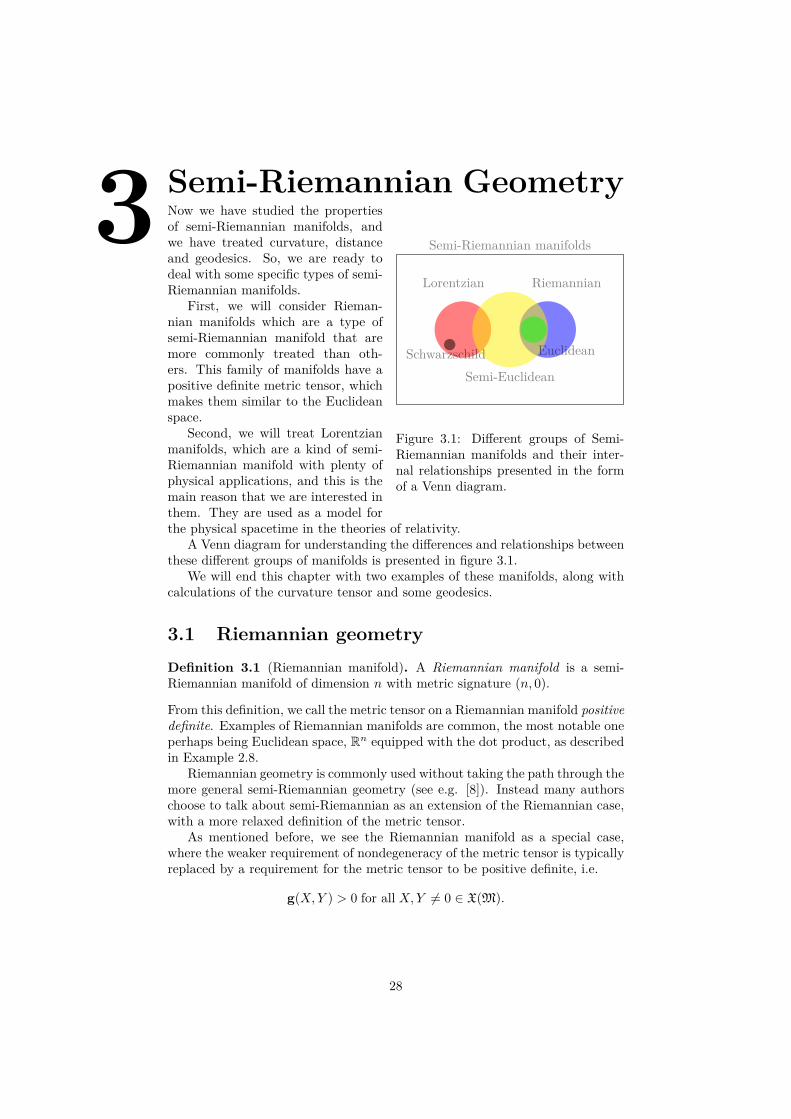
Figure 3.1: Different groups of Semi-Riemannian manifolds and their inter-nal relationships presented in the formof a Venn diagram.

Now we have studied the propertiesof semi-Riemannian manifolds, andwe have treated curvature, distanceand geodesics. So, we are ready todeal with some specific types of semi-Riemannian manifolds.

First, we will consider Rieman-nian manifolds which are a type ofsemi-Riemannian manifold that aremore commonly treated than oth-ers. This family of manifolds have apositive definite metric tensor, whichmakes them similar to the Euclideanspace.

Second, we will treat Lorentzianmanifolds, which are a kind of semi-Riemannian manifold with plenty ofphysical applications, and this is themain reason that we are interested inthem. They are used as a model forthe physical spacetime in the theories of relativity.

A Venn diagram for understanding the differences and relationships betweenthese different groups of manifolds is presented in figure 3.1.

We will end this chapter with two examples of these manifolds, along withcalculations of the curvature tensor and some geodesics.

3.1 Riemannian geometryDefinition 3.1 (Riemannian manifold). A Riemannian manifold is a semi-Riemannian manifold of dimension n with metric signature (n, 0).

From this definition, we call the metric tensor on a Riemannian manifold positivedefinite. Examples of Riemannian manifolds are common, the most notable oneperhaps being Euclidean space, Rn equipped with the dot product, as describedin Example 2.8.

Riemannian geometry is commonly used without taking the path through themore general semi-Riemannian geometry (see e.g. [8]). Instead many authorschoose to talk about semi-Riemannian as an extension of the Riemannian case,with a more relaxed definition of the metric tensor.

As mentioned before, we see the Riemannian manifold as a special case,where the weaker requirement of nondegeneracy of the metric tensor is typicallyreplaced by a requirement for the metric tensor to be positive definite, i.e.

g(X,Y ) > 0 for all X,Y 6= 0 ∈ X(M).

28

3.2 Lorentzian geometryWe will now consider Lorentzian manifolds, a type of semi-Riemannian manifoldthat is used extensively to model the physical spacetime of the universe. In thissection, we give a concise summary of the way we will look at vectors and curvesin Lorentzian manifolds. The reader of a mathematical persuasion may thinkof lightlike, causal future and so on as merely mathematical label. The physicalmathematician may think of these families of vectors and curves as related tophysical reality.

Definition 3.2 (Lorentzian manifold). A Lorentzian manifold is a semi-Rieman-nian manifold of dimension n with metric signature (1, n− 1).

Definition 3.3 (Causal character of tangent vectors). On a Lorentzian mani-fold M with metric tensor g, a tangent vector Xp is spacelike, null or timelike,characterized accordingly:

i. Timelike:〈Xp, Xp〉 > 0 while Xp 6= 0, otherwise 〈Xp, Xp〉 = 0,

ii. Null or lightlike:〈Xp, Xp〉 = 0 and Xp 6= 0,

iii. Spacelike:〈Xp, Xp〉 < 0.

This could be called the way we measure the length of a vector onM. Perhaps weneed to extend our view of what length is, since a nonzero vector can have zerolength. This is significant both mathematically and physically. Mathematically,by Nash’s embedding theorem, any N -dimensional Riemannian manifold can beisometrically embedded into Rn ([14]). However, this is definitely not true forLorentzian manifolds.

What we mean by isometrical embedding here is that there exists a func-tion on every N -dimensional Riemannian manifold M, f : M → Rn such thatg(X,Y ) = g(df(X), df(Y )). This describes an embedding of the metric of aRiemannian manifold. In this it differs from (but is based on) the Whitney em-bedding theorem, which describes the embedding of a manifold and its tangentbundle ([22]).

Remember the definition of a semi-Euclidean space Rnν (Example 2.9) andthat in particular, R1

3 is called a Minkowski space. Note that many other authorsvary this notation by denoting a semi-Euclidean space by (in our system) R(n+ν)

ν

or sometimes the sign convention is reversed so that it is written Rν(n+ν).Now, what is interesting about the mathematical perspective of an N -

dimensional Lorentzian manifold is that it cannot in general be embedded ina R1

n manifold, sometimes called Ln ([13]). However, any N -dimensional semi-Riemannian manifold can be isometrically embedded into the semi-Euclideanspace Rnν , of sufficiently large n and ν ([13]). Lorentzian manifolds are alsointeresting from a physical perspective due to the applications of Lorentzianmanifolds to relativity. It is from this perspective that the previous definitionof the causal character of vectors becomes interesting.

29

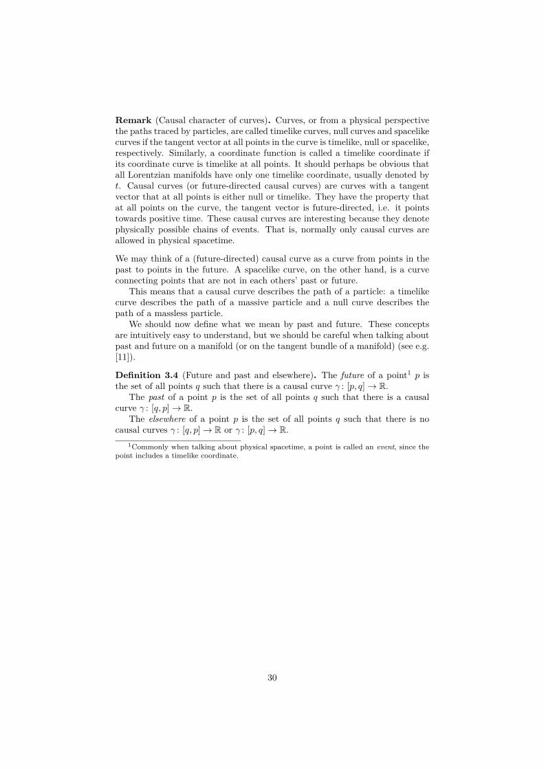
Remark (Causal character of curves). Curves, or from a physical perspectivethe paths traced by particles, are called timelike curves, null curves and spacelikecurves if the tangent vector at all points in the curve is timelike, null or spacelike,respectively. Similarly, a coordinate function is called a timelike coordinate ifits coordinate curve is timelike at all points. It should perhaps be obvious thatall Lorentzian manifolds have only one timelike coordinate, usually denoted byt. Causal curves (or future-directed causal curves) are curves with a tangentvector that at all points is either null or timelike. They have the property thatat all points on the curve, the tangent vector is future-directed, i.e. it pointstowards positive time. These causal curves are interesting because they denotephysically possible chains of events. That is, normally only causal curves areallowed in physical spacetime.

We may think of a (future-directed) causal curve as a curve from points in thepast to points in the future. A spacelike curve, on the other hand, is a curveconnecting points that are not in each others’ past or future.

This means that a causal curve describes the path of a particle: a timelikecurve describes the path of a massive particle and a null curve describes thepath of a massless particle.

We should now define what we mean by past and future. These conceptsare intuitively easy to understand, but we should be careful when talking aboutpast and future on a manifold (or on the tangent bundle of a manifold) (see e.g.[11]).

Definition 3.4 (Future and past and elsewhere). The future of a point1 p isthe set of all points q such that there is a causal curve γ : [p, q]→ R.

The past of a point p is the set of all points q such that there is a causalcurve γ : [q, p]→ R.

The elsewhere of a point p is the set of all points q such that there is nocausal curves γ : [q, p]→ R or γ : [p, q]→ R.

1Commonly when talking about physical spacetime, a point is called an event, since thepoint includes a timelike coordinate.

30

Past

ct

xHyperspace of the present

y

Elsewhere

Future

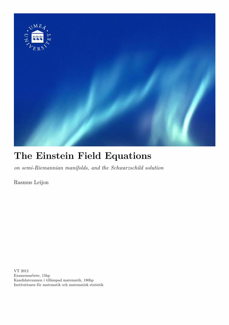
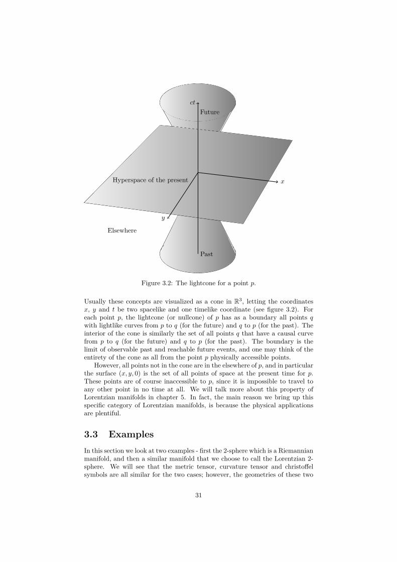
Figure 3.2: The lightcone for a point p.

Usually these concepts are visualized as a cone in R3, letting the coordinatesx, y and t be two spacelike and one timelike coordinate (see figure 3.2). Foreach point p, the lightcone (or nullcone) of p has as a boundary all points qwith lightlike curves from p to q (for the future) and q to p (for the past). Theinterior of the cone is similarly the set of all points q that have a causal curvefrom p to q (for the future) and q to p (for the past). The boundary is thelimit of observable past and reachable future events, and one may think of theentirety of the cone as all from the point p physically accessible points.

However, all points not in the cone are in the elsewhere of p, and in particularthe surface (x, y, 0) is the set of all points of space at the present time for p.These points are of course inaccessible to p, since it is impossible to travel toany other point in no time at all. We will talk more about this property ofLorentzian manifolds in chapter 5. In fact, the main reason we bring up thisspecific category of Lorentzian manifolds, is because the physical applicationsare plentiful.

3.3 ExamplesIn this section we look at two examples - first the 2-sphere which is a Riemannianmanifold, and then a similar manifold that we choose to call the Lorentzian 2-sphere. We will see that the metric tensor, curvature tensor and christoffelsymbols are all similar for the two cases; however, the geometries of these two

31

manifolds are very different.

Example 3.5 (Riemannian 2-sphere). Consider a two-dimensional Riemannianmanifold M with some coordinate system

(U , φ = (u, v)

).

Let the metric tensor g be positive definite, with components be given by:

gαβ =[1 00 sin2 u

]and therefore also length segment: ds2 = du2 + sin2 udv2, and metric signature(2, 0).

This leads to the nonzero Christoffel symbols:

Γuvv = − sin u cosu, Γvuv = Γvvu = cosusin u .

Now, these coordinates are clearly orthogonal, letting us simplify the geodesicequations to the equations in Example 3.2.

In this metric, any vector fields X is positive definite, that is∑α

∑β

gαβXαXβ > 0,

for X not a zero vector, because:∑α

∑β

gαβXαXβ =

∑α

gααXαXα = (Xu)2 + sin2 u (Xv)2

.

This is clearly always positive-definite, which is defining for the Riemanniangeometry.

Noting that only ∂ugvv 6= 0, the sum in the equation disappears and we gettwo equations:

d

ds

(du

ds

)− sin u cosu

(dv

ds

)2= 0,

d

ds

(sin2 u

dv

ds

)= 0.

Without attempting to solve them, we can see that a curve γ(s) = (u(s), v(s)) =(s, v0), v0 constant, satisfies these equations and is therefore a geodesic on thisRiemannian manifold.

Looking at the curvature tensor, after some tedious but simple calculationswe can derive that it has, relative to (u, v), four nonzero components:

Ruvuv = − sin2 u, Ruvvu = sin2 u,

Rvuvu = −1, Rvuuv = 1.

We may notice that the Riemannian manifold is not flat, but has ‘a little’curvature. This should come as no surprise, since the components of the metrictensor are not constant.

Now that we have explored many of the properties of this manifold, we willcontinue to the less intuitive case of a Lorentzian manifold.

32

Example 3.6 (Lorentzian 2-sphere). Consider a two-dimensional Lorentzianmanifold M with some coordinate system φ = (u, v), much like the previousRiemannian manifold.

Unlike the Riemannian manifold, however, this Lorentzian manifold has met-ric signature (1, 1). Now, let the metric tensor g be indefinite, with componentsbe given by:

gαβ =[1 00 − sin2 u

]Now, the question arises: what is the difference between these geometries? Well,it is clear that the line segment takes a different form:

ds2 = du2 − sin2 udv2,

and it is clear that some counterintuitive properties follow from allowing thatminus sign!

33

4 The Einstein Field EquationsWe are now ready to treat the physical applications of semi-Riemannian man-ifolds. Since we started discussing semi-Riemannian manifolds, we have dis-cussed measurement of distance and curvature. In this chapter, we apply theresults of these theorems and the categorizations of semi-Riemannian manifoldsfrom chapter 3.

In this chapter, we view the physical universe as a 4-dimensional Lorentzianmanifold, eventually postulating the Einstein field equations, which formulatethe relation between curvature and stress-energy content in the universe. Thisallows us to view the curvature tensor as a physical property of the universe, asa function of mass, momentum and energy.

Solving these equations through our main theorem, we can find the metrictensor for this manifold which allows us to, for example, formulate the geodesicequations, which describe straight paths through the physical spacetime. Thesetwo theorems are fundamental for our understanding of how semi-Riemannianmanifolds relate to physics, and from a mathematical perspective they can beseen as a useful and in-depth example of problems that can be formulated andsolved on a semi-Riemannian manifold.

This solution that we present, the Schwarzschild solution, has many usefulapplications in practice, and we shall show in the next chapter that it can de-scribe the orbits of celestial bodies with increased accuracy over the Newtonianmodel. However, we start by formulating the special theory of relativity interms of semi-Riemannian geometry before generalizing.

4.1 Special relativityThe special theory of relativity is a generalization of the Newtonian mechanicsand electrodynamics to high velocities. It is based upon two principles: that inall inertial reference frames the laws of physics have the same form and that inall inertial reference frames, the speed of light in a vacuum are the same.

The special theory of relativity is modelled as the four-dimensional Minkows-ki spacetime, M = R1

3. One significant aspect when studying the motion of aparticle in the special theory of relativity is that and even though we still havethe timelike coordinate t, we cannot talk about t as some form of objective timefor the particle’s movement (see e.g. [11] or [4]).

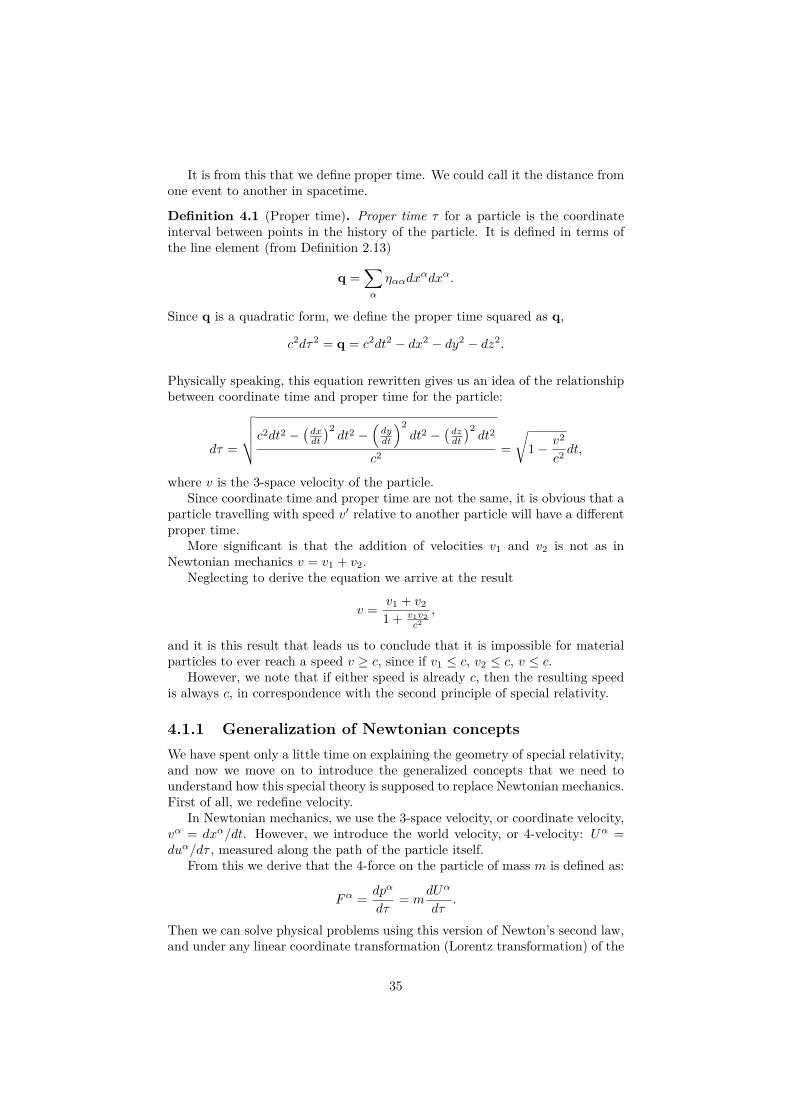
Instead, we call t coordinate time, and use a different function, τ , to denotewhat we call proper time. This proper time is the time as measured by theparticle itself, that is, in an inertial reference frame where the particle appearsto be at rest.

Now, since M = R13, the metric tensor of M is usually called η, with com-

ponents given by:

ηαβ =

1 0 0 00 −1 0 00 0 −1 00 0 0 −1

This gives us the line element in the coordinate system φ = (ct, x, y, z): ds2 =c2dt2 − dx2 − dy2 − dz2.

34

It is from this that we define proper time. We could call it the distance fromone event to another in spacetime.

Definition 4.1 (Proper time). Proper time τ for a particle is the coordinateinterval between points in the history of the particle. It is defined in terms ofthe line element (from Definition 2.13)

q =∑α

ηααdxαdxα.

Since q is a quadratic form, we define the proper time squared as q,

c2dτ2 = q = c2dt2 − dx2 − dy2 − dz2.

Physically speaking, this equation rewritten gives us an idea of the relationshipbetween coordinate time and proper time for the particle:

dτ =

√√√√c2dt2 −(dxdt

)2dt2 −

(dydt

)2dt2 −

(dzdt

)2dt2

c2=√

1− v2

c2dt,

where v is the 3-space velocity of the particle.Since coordinate time and proper time are not the same, it is obvious that a

particle travelling with speed v′ relative to another particle will have a differentproper time.

More significant is that the addition of velocities v1 and v2 is not as inNewtonian mechanics v = v1 + v2.

Neglecting to derive the equation we arrive at the result

v = v1 + v2

1 + v1v2c2

,

and it is this result that leads us to conclude that it is impossible for materialparticles to ever reach a speed v ≥ c, since if v1 ≤ c, v2 ≤ c, v ≤ c.

However, we note that if either speed is already c, then the resulting speedis always c, in correspondence with the second principle of special relativity.

4.1.1 Generalization of Newtonian conceptsWe have spent only a little time on explaining the geometry of special relativity,and now we move on to introduce the generalized concepts that we need tounderstand how this special theory is supposed to replace Newtonian mechanics.First of all, we redefine velocity.

In Newtonian mechanics, we use the 3-space velocity, or coordinate velocity,vα = dxα/dt. However, we introduce the world velocity, or 4-velocity: Uα =duα/dτ , measured along the path of the particle itself.

From this we derive that the 4-force on the particle of mass m is defined as:

Fα = dpα

dτ= m

dUα

dτ.

Then we can solve physical problems using this version of Newton’s second law,and under any linear coordinate transformation (Lorentz transformation) of the

35

coordinates φ = uα, it is required from the first principle of special relativitythat these laws are invariant. These transformations can be written in terms ofthe coordinates as

uα =∑β

Λαβuβ + cα, (4.1)

where Λ is required to satisfy∑α

∑β

ηαβΛαµΛβν = ηµν .

It can be shown that these laws hold up under the transformations (4.1),however we focus on the shortcomings of the special theory; namely, that theforce felt from gravity by a particle is not in general the same for two differentobservers (see e.g. chapter 2 in [11]).

This inconsistency required the formulation of a theory that incorporatesgravity into the relativistic framework.

4.2 General relativityThe general theory of relativity in turn generalizes the special theory of relativ-ity, and in particular it describes the force of gravity as well as all the effectsof special relativity, by using a semi-Riemannian manifold of metric signature(1, 3). It models the effects of gravity as the curvature of this manifold.

It of course also generalizes the special theory of relativity by using an ingeneral non-flat metric tensor, and in fact is required to approximate to specialrelativity locally. Special relativity is a special case of general relativity, wherethere is no gravitational force acting on the particle.

The general theory of relativity models the universe as a spacetime, a (1, 3)Lorentzian manifold with a metric tensor which is not flat in general, but variesaccording to a few fundamental principles. The general theory is foremost ageneralization of the special theory, and depends on the postulates of the specialtheory.

Equivalence principleThe equivalence principle states that for a from-infinity nonrotating smallneighborhood of spacetime on which the force of gravity is the only forceacting upon it, the laws of physics are the laws of special relativity.Since there is now no distinction between a particle at rest in a gravita-tional field and a particle accelerated by a force equal to gravity, we cancategorize the motion of objects in free fall under the influence of gravityas travelling along geodesics on the spacetime manifold.

Energy-momentum curves spacetimeThe curvature of the Lorentzian manifold of spacetime is caused by energy-momentum. Since geodesics on this manifold are motions of particlesin free fall; that is, only affected by the force of gravity, curvature andgravitation are linked.The source of gravity is energy-momentum, and the source of curvature inthis manifold is gravity. The precise equation for this relation is describedlater in this section, and is the foundation of general relativity.

36

4.2.1 The Einstein field equationsFirst, we have decided that energy-momentum curves spacetime. We will workwith a manifoldM with metric signature (1, 3) and metric tensor g. It is obviousthat the equations governing the relation between curvature and and energy-momentum should contain some form of the curvature tensor and some form oftensor energy-momentum tensor (see e.g. [11]).

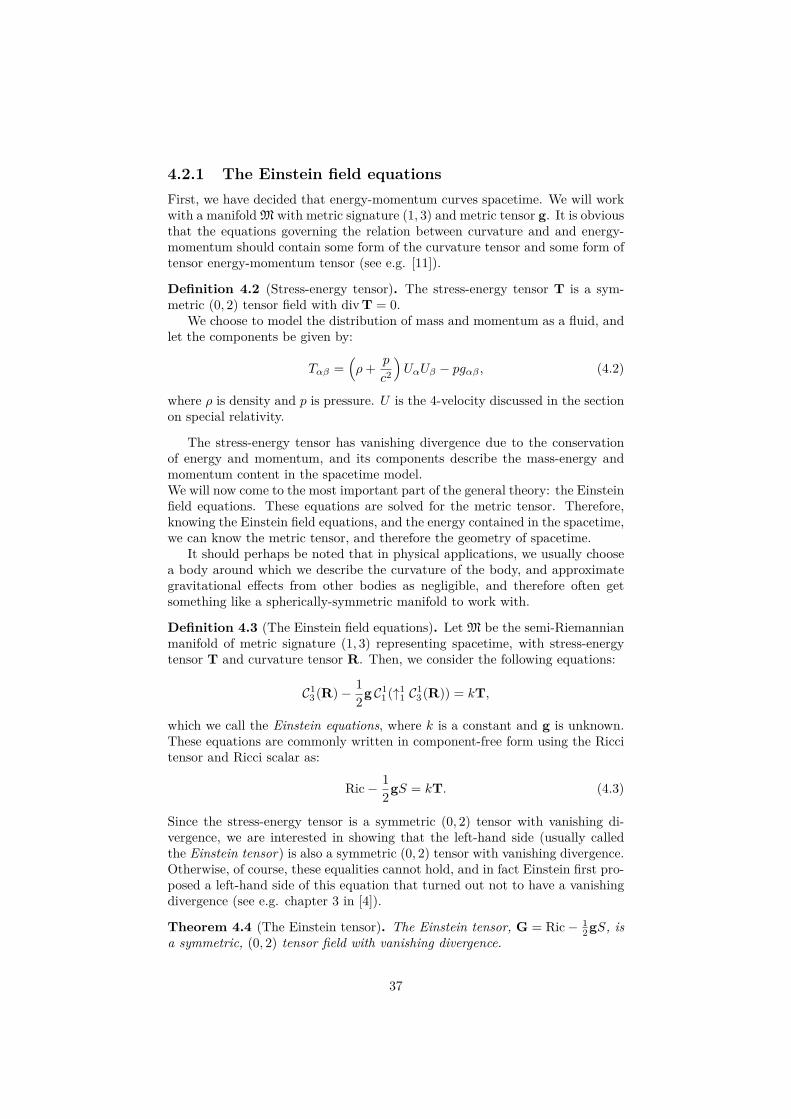
Definition 4.2 (Stress-energy tensor). The stress-energy tensor T is a sym-metric (0, 2) tensor field with div T = 0.

We choose to model the distribution of mass and momentum as a fluid, andlet the components be given by:

Tαβ =(ρ+ p

c2

)UαUβ − pgαβ , (4.2)

where ρ is density and p is pressure. U is the 4-velocity discussed in the sectionon special relativity.

The stress-energy tensor has vanishing divergence due to the conservationof energy and momentum, and its components describe the mass-energy andmomentum content in the spacetime model.We will now come to the most important part of the general theory: the Einsteinfield equations. These equations are solved for the metric tensor. Therefore,knowing the Einstein field equations, and the energy contained in the spacetime,we can know the metric tensor, and therefore the geometry of spacetime.

It should perhaps be noted that in physical applications, we usually choosea body around which we describe the curvature of the body, and approximategravitational effects from other bodies as negligible, and therefore often getsomething like a spherically-symmetric manifold to work with.

Definition 4.3 (The Einstein field equations). Let M be the semi-Riemannianmanifold of metric signature (1, 3) representing spacetime, with stress-energytensor T and curvature tensor R. Then, we consider the following equations:

C13(R)− 1

2g C11(↑11 C1

3(R)) = kT,

which we call the Einstein equations, where k is a constant and g is unknown.These equations are commonly written in component-free form using the Riccitensor and Ricci scalar as:

Ric− 12gS = kT. (4.3)

Since the stress-energy tensor is a symmetric (0, 2) tensor with vanishing di-vergence, we are interested in showing that the left-hand side (usually calledthe Einstein tensor) is also a symmetric (0, 2) tensor with vanishing divergence.Otherwise, of course, these equalities cannot hold, and in fact Einstein first pro-posed a left-hand side of this equation that turned out not to have a vanishingdivergence (see e.g. chapter 3 in [4]).

Theorem 4.4 (The Einstein tensor). The Einstein tensor, G = Ric− 12gS, is

a symmetric, (0, 2) tensor field with vanishing divergence.

37

Proof. First we prove that G is a (0, 2) tensor field: That it is a (0, 2) tensorfield is clear from the fact that g is a (0, 2) tensor and from the definition ofcontraction, the contraction of the (1, 3) tensor R is C1

3(R) ∈ T02(M).

Now we prove that G is symmetric: Since g is symmetric and by Lemma 2.30,the Ricci tensor is symmetric, G is clearly symmetric.

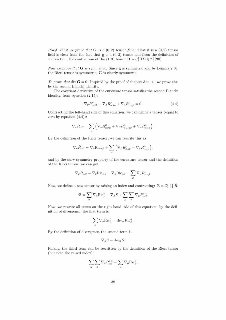
To prove that div G = 0: Inspired by the proof of chapter 3 in [4], we prove thisby the second Bianchi identity.

The covariant derivative of the curvature tensor satisfies the second Bianchiidentity, from equation (2.15):

∇νRµαβλ +∇βRµαλν +∇λRµανβ = 0. (4.4)

Contracting the left-hand side of this equation, we can define a tensor (equal tozero by equation (4.4)):

∇νRαβ =∑µ

(∇νRµαβµ +∇βRµαµν;β +∇µRµανβ

).

By the definition of the Ricci tensor, we can rewrite this as

∇νRαβ = ∇νRicαβ +∑µ

(∇βRµαµν −∇µR

µανβ

),

and by the skew-symmetry property of the curvature tensor and the definitionof the Ricci tensor, we can get

∇νRαβ = ∇νRicαβ −∇βRicαν +∑µ

∇µRµανβ .

Now, we define a new tensor by raising an index and contracting: R = C12 ↑11 R,

R =∑α

∇αRicαβ −∇βS +∑µ

∑α

∇µRµααβ .

Now, we rewrite all terms on the right-hand side of this equation: by the defi-nition of divergence, the first term is∑

α

∇αRicαβ = divα Ricαβ .

By the definition of divergence, the second term is

∇βS = divβ S.

Finally, the third term can be rewritten by the definition of the Ricci tensor(but note the raised index):∑

µ

∑α

∇µRµααβ =∑µ

∇µRicµβ ,

38

and by the definition of the divergence, this is divµRicµβ . Now, just rewriting Rby changing the label in the third term from µ to α it becomes

R =∑α

∇α(

Ricαβ −12Sδ

αβ

),

where δαβ is the Kronecker delta. By the definition of divergence, this is:

R = divα(

Ricαβ −12Sδ

αβ

).

Now, by the definition of the Einstein tensor:

Ricαβ −12Sδ

αβ =↑11 G.

Finally, from the second Bianchi identity (4.4), we get that

div ↑11 G = 0

This proves that the Einstein tensor G has a vanishing divergence.

Now that we have established this relation between curvature and energy, wecan delve into the solution for these equations in Theorem 4.8 in the comingsection.

4.3 The Schwarzschild geometryThe first solution to the Einstein field equations presented was the Schwarzschildsolution. It is the most general solution for the physical spacetime surrounding astatic, spherically symmetric, uncharged, at infinity non-rotating massive body,such as a star with negligible rotational energy1 (see e.g. chapter 23 in [11]).

We therefore look at the 4-dimensional Lorentzian manifold M with thetopology of R4. Now, we more rigorously investigate the geometric and topo-logical properties of the Schwarzschild spacetime. It is common to define thegeometry of a semi-Riemannian manifold in terms of the line element q (seeDefinition 2.13).

1. The physical spacetime is given to be static.

What we mean by static is that the geometry of M does not depend onany timelike coordinate function.For this reason, we will model our four-dimensional spacetime as a semi-Riemannian product manifold R×R3 with a metric tensor that does notdepend on the timelike coordinate. Using Euclidean space (Example 2.8)as a model for our spacelike coordinates, we can write the line element qas

q = A(x, y, z)c2dt2 − B(x, y, z)dx2 − C(x, y, z)dy2 − D(x, y, z)dz2,

1The spacetime outside of our own star is a good approximation to this kind of spacetime,even though the sun has some rotational energy.

39

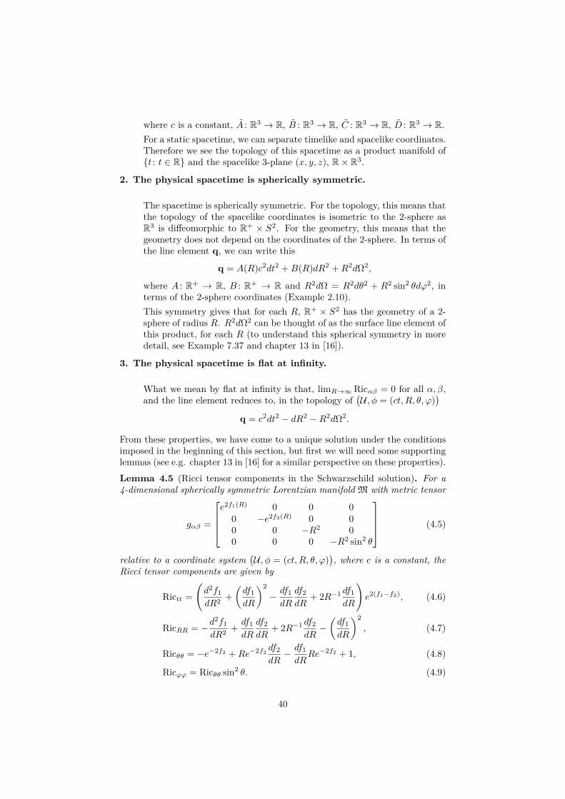
where c is a constant, A : R3 → R, B : R3 → R, C : R3 → R, D : R3 → R.For a static spacetime, we can separate timelike and spacelike coordinates.Therefore we see the topology of this spacetime as a product manifold oft : t ∈ R and the spacelike 3-plane (x, y, z), R× R3.

2. The physical spacetime is spherically symmetric.

The spacetime is spherically symmetric. For the topology, this means thatthe topology of the spacelike coordinates is isometric to the 2-sphere asR3 is diffeomorphic to R+ × S2. For the geometry, this means that thegeometry does not depend on the coordinates of the 2-sphere. In terms ofthe line element q, we can write this

q = A(R)c2dt2 +B(R)dR2 +R2dΩ2,

where A : R+ → R, B : R+ → R and R2dΩ = R2dθ2 + R2 sin2 θdϕ2, interms of the 2-sphere coordinates (Example 2.10).This symmetry gives that for each R, R+ × S2 has the geometry of a 2-sphere of radius R. R2dΩ2 can be thought of as the surface line element ofthis product, for each R (to understand this spherical symmetry in moredetail, see Example 7.37 and chapter 13 in [16]).

3. The physical spacetime is flat at infinity.

What we mean by flat at infinity is that, limR→∞Ricαβ = 0 for all α, β,and the line element reduces to, in the topology of

(U , φ = (ct, R, θ, ϕ)

)q = c2dt2 − dR2 −R2dΩ2.

From these properties, we have come to a unique solution under the conditionsimposed in the beginning of this section, but first we will need some supportinglemmas (see e.g. chapter 13 in [16] for a similar perspective on these properties).Lemma 4.5 (Ricci tensor components in the Schwarzschild solution). For a4-dimensional spherically symmetric Lorentzian manifold M with metric tensor

gαβ =

e2f1(R) 0 0 0

0 −e2f2(R) 0 00 0 −R2 00 0 0 −R2 sin2 θ

(4.5)

relative to a coordinate system(U , φ = (ct, R, θ, ϕ)

), where c is a constant, the

Ricci tensor components are given by

Rictt =(d2f1

dR2 +(df1

dR

)2− df1

dR

df2

dR+ 2R−1 df1

dR

)e2(f1−f2), (4.6)

RicRR = −d2f1

dR2 + df1

dR

df2

dR+ 2R−1 df2

dR−(df1

dR

)2, (4.7)

Ricθθ = −e−2f2 +Re−2f2df2

dR− df1

dRRe−2f2 + 1, (4.8)

Ricϕϕ = Ricθθ sin2 θ. (4.9)

40

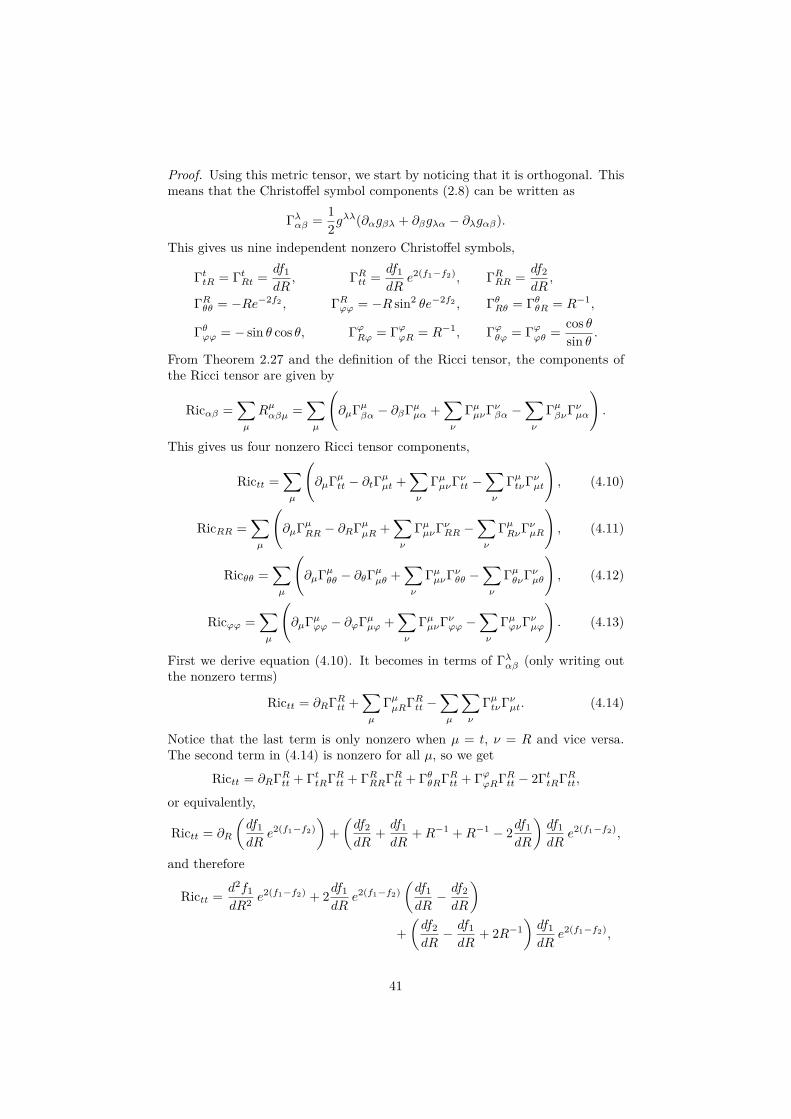
Proof. Using this metric tensor, we start by noticing that it is orthogonal. Thismeans that the Christoffel symbol components (2.8) can be written as

Γλαβ = 12g

λλ(∂αgβλ + ∂βgλα − ∂λgαβ).

This gives us nine independent nonzero Christoffel symbols,

ΓttR = ΓtRt = df1

dR, ΓRtt = df1

dRe2(f1−f2), ΓRRR = df2

dR,

ΓRθθ = −Re−2f2 , ΓRϕϕ = −R sin2 θe−2f2 , ΓθRθ = ΓθθR = R−1,

Γθϕϕ = − sin θ cos θ, ΓϕRϕ = ΓϕϕR = R−1, Γϕθϕ = Γϕϕθ = cos θsin θ .

From Theorem 2.27 and the definition of the Ricci tensor, the components ofthe Ricci tensor are given by

Ricαβ =∑µ

Rµαβµ =∑µ

(∂µΓµβα − ∂βΓµµα +

∑ν

ΓµµνΓνβα −∑ν

ΓµβνΓνµα

).

This gives us four nonzero Ricci tensor components,

Rictt =∑µ

(∂µΓµtt − ∂tΓ

µµt +

∑ν

ΓµµνΓνtt −∑ν

ΓµtνΓνµt

), (4.10)

RicRR =∑µ

(∂µΓµRR − ∂RΓµµR +

∑ν

ΓµµνΓνRR −∑ν

ΓµRνΓνµR

), (4.11)

Ricθθ =∑µ

(∂µΓµθθ − ∂θΓ

µµθ +

∑ν

ΓµµνΓνθθ −∑ν

ΓµθνΓνµθ

), (4.12)

Ricϕϕ =∑µ

(∂µΓµϕϕ − ∂ϕΓµµϕ +

∑ν

ΓµµνΓνϕϕ −∑ν

ΓµϕνΓνµϕ

). (4.13)

First we derive equation (4.10). It becomes in terms of Γλαβ (only writing outthe nonzero terms)

Rictt = ∂RΓRtt +∑µ

ΓµµRΓRtt −∑µ

∑ν

ΓµtνΓνµt. (4.14)

Notice that the last term is only nonzero when µ = t, ν = R and vice versa.The second term in (4.14) is nonzero for all µ, so we get

Rictt = ∂RΓRtt + ΓttRΓRtt + ΓRRRΓRtt + ΓθθRΓRtt + ΓϕϕRΓRtt − 2ΓttRΓRtt,

or equivalently,

Rictt = ∂R

(df1

dRe2(f1−f2)

)+(df2

dR+ df1

dR+R−1 +R−1 − 2df1

dR

)df1

dRe2(f1−f2),

and therefore

Rictt = d2f1

dR2 e2(f1−f2) + 2df1

dRe2(f1−f2)

(df1

dR− df2

dR

)+(df2

dR− df1

dR+ 2R−1

)df1

dRe2(f1−f2),

41

or simply

Rictt =(d2f1

dR2 +(df1

dR

)2− df1

dR

df2

dR+ 2R−1 df1

dR

)e2(f1−f2).

This proves that the tt-component of the Ricci tensor is equal to (4.6).Now we derive equation (4.11). In terms of Γλαβ (again only writing out thenonzero terms) we have

RicRR = ∂RΓRRR − ∂R(

ΓttR + ΓRRR + ΓθθR + ΓϕϕR)

+∑µ

∑ν

ΓµµνΓνRR −∑µ

∑ν

ΓµRνΓνµR.

Clearly the third term is only nonzero for ν = R. The fourth term is onlynonzero for µ = ν. This gives us

RicRR = ∂RΓRRR − ∂R(

ΓttR + ΓRRR + ΓθθR + ΓϕϕR)

+(

ΓttR + ΓRRR + ΓθθR + ΓϕϕR)

ΓRRR

−(

ΓttRΓttR + ΓRRRΓRRR + ΓθθRΓθθR + ΓϕϕRΓϕϕR).

or in terms of the metric tensor components,

RicRR = d2f2

dR2 − ∂R(df1

dR+ df2

dR+R−1 +R−1

)+(df1

dR+ df2

dR+R−1 +R−1

)df2

dR

−

((df1

dR

)2+(df2

dR

)2+R−2 +R−2

).

or equivalently,

RicRR = −d2f1

dR2 + df1

dR

df2

dR+ 2R−1 df2

dR−(df1

dR

)2.

This concludes the proof of equation (4.7).Next, we shall derive equation (4.12). Again in terms of the non-zero Christoffelsymbols, we get:

Ricθθ = ∂RΓRθθ − ∂θΓϕϕθ +

∑µ

(∑ν

ΓµµνΓνθθ −∑ν

ΓµθνΓνµθ

).

In the third term, clearly only for ν = R is the term nonzero. The fourth termis nonzero in three cases: for µ = θ, ν = R (and vice versa), and for µ = ν = ϕ.Considering this, the previous equation becomes

Ricθθ = ∂RΓRθθ − ∂θΓϕϕθ +

(ΓttR + ΓRRR + ΓθθR + ΓϕϕR

)ΓRθθ −

(Γϕθϕ

)2− 2ΓθθRΓRθθ.

42

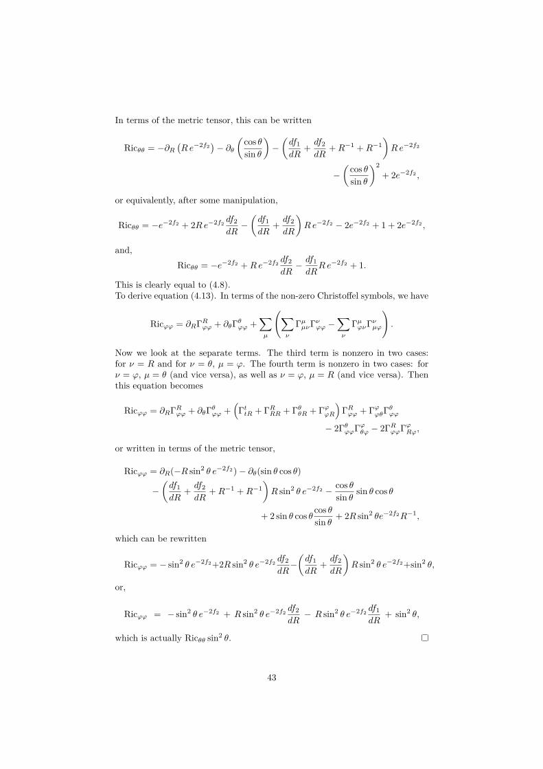
In terms of the metric tensor, this can be written

Ricθθ = −∂R(Re−2f2

)− ∂θ

(cos θsin θ

)−(df1

dR+ df2

dR+R−1 +R−1

)Re−2f2

−(

cos θsin θ

)2+ 2e−2f2 ,

or equivalently, after some manipulation,

Ricθθ = −e−2f2 + 2Re−2f2df2

dR−(df1

dR+ df2

dR

)Re−2f2 − 2e−2f2 + 1 + 2e−2f2 ,

and,Ricθθ = −e−2f2 +Re−2f2

df2

dR− df1

dRRe−2f2 + 1.

This is clearly equal to (4.8).To derive equation (4.13). In terms of the non-zero Christoffel symbols, we have

Ricϕϕ = ∂RΓRϕϕ + ∂θΓθϕϕ +∑µ

(∑ν

ΓµµνΓνϕϕ −∑ν

ΓµϕνΓνµϕ

).

Now we look at the separate terms. The third term is nonzero in two cases:for ν = R and for ν = θ, µ = ϕ. The fourth term is nonzero in two cases: forν = ϕ, µ = θ (and vice versa), as well as ν = ϕ, µ = R (and vice versa). Thenthis equation becomes

Ricϕϕ = ∂RΓRϕϕ + ∂θΓθϕϕ +(

ΓttR + ΓRRR + ΓθθR + ΓϕϕR)

ΓRϕϕ + ΓϕϕθΓθϕϕ

− 2ΓθϕϕΓϕθϕ − 2ΓRϕϕΓϕRϕ,

or written in terms of the metric tensor,

Ricϕϕ = ∂R(−R sin2 θ e−2f2)− ∂θ(sin θ cos θ)

−(df1

dR+ df2

dR+R−1 +R−1

)R sin2 θ e−2f2 − cos θ

sin θ sin θ cos θ

+ 2 sin θ cos θ cos θsin θ + 2R sin2 θe−2f2R−1,

which can be rewritten

Ricϕϕ = − sin2 θ e−2f2+2R sin2 θ e−2f2df2

dR−(df1

dR+ df2

dR

)R sin2 θ e−2f2+sin2 θ,

or,

Ricϕϕ = − sin2 θ e−2f2 + R sin2 θ e−2f2df2

dR− R sin2 θ e−2f2

df1

dR+ sin2 θ,

which is actually Ricθθ sin2 θ.

43

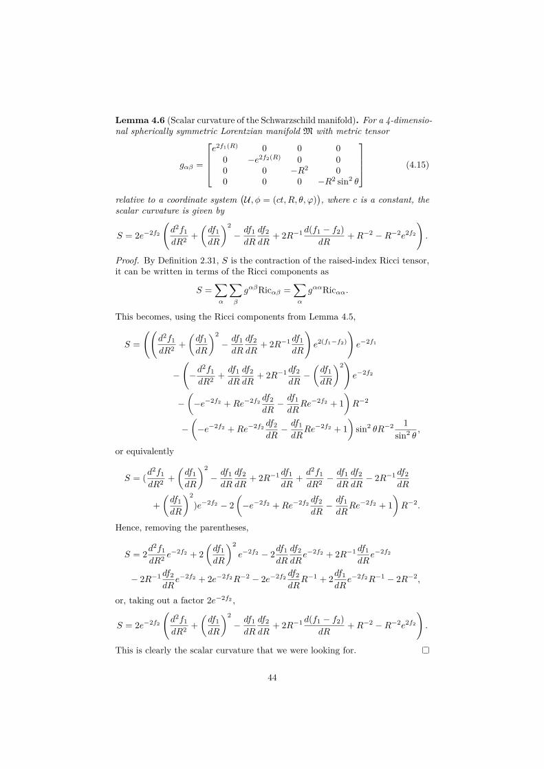
Lemma 4.6 (Scalar curvature of the Schwarzschild manifold). For a 4-dimensio-nal spherically symmetric Lorentzian manifold M with metric tensor

gαβ =

e2f1(R) 0 0 0

0 −e2f2(R) 0 00 0 −R2 00 0 0 −R2 sin2 θ

(4.15)

relative to a coordinate system(U , φ = (ct, R, θ, ϕ)

), where c is a constant, the

scalar curvature is given by

S = 2e−2f2

(d2f1

dR2 +(df1

dR

)2− df1

dR

df2

dR+ 2R−1 d(f1 − f2)

dR+R−2 −R−2e2f2

).

Proof. By Definition 2.31, S is the contraction of the raised-index Ricci tensor,it can be written in terms of the Ricci components as

S =∑α

∑β

gαβRicαβ =∑α

gααRicαα.

This becomes, using the Ricci components from Lemma 4.5,

S =((

d2f1

dR2 +(df1

dR

)2− df1

dR

df2

dR+ 2R−1 df1

dR

)e2(f1−f2)

)e−2f1

−

(−d

2f1

dR2 + df1

dR

df2

dR+ 2R−1 df2

dR−(df1

dR

)2)e−2f2

−(−e−2f2 +Re−2f2

df2

dR− df1

dRRe−2f2 + 1

)R−2

−(−e−2f2 +Re−2f2

df2

dR− df1

dRRe−2f2 + 1

)sin2 θR−2 1

sin2 θ,

or equivalently

S = (d2f1

dR2 +(df1

dR

)2− df1

dR

df2

dR+ 2R−1 df1

dR+ d2f1

dR2 −df1

dR

df2

dR− 2R−1 df2

dR

+(df1

dR

)2)e−2f2 − 2

(−e−2f2 +Re−2f2

df2

dR− df1

dRRe−2f2 + 1

)R−2.

Hence, removing the parentheses,

S = 2d2f1

dR2 e−2f2 + 2

(df1

dR

)2e−2f2 − 2df1

dR

df2

dRe−2f2 + 2R−1 df1

dRe−2f2

− 2R−1 df2

dRe−2f2 + 2e−2f2R−2 − 2e−2f2

df2

dRR−1 + 2df1

dRe−2f2R−1 − 2R−2,

or, taking out a factor 2e−2f2 ,

S = 2e−2f2

(d2f1

dR2 +(df1

dR

)2− df1

dR

df2

dR+ 2R−1 d(f1 − f2)

dR+R−2 −R−2e2f2

).

This is clearly the scalar curvature that we were looking for.

44

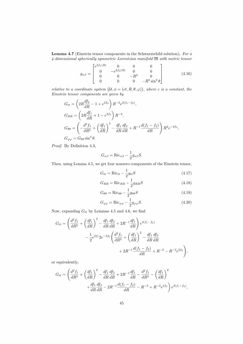
Lemma 4.7 (Einstein tensor components in the Schwarzschild solution). For a4-dimensional spherically symmetric Lorentzian manifold M with metric tensor

gαβ =

e2f1(R) 0 0 0

0 −e2f2(R) 0 00 0 −R2 00 0 0 −R2 sin2 θ

(4.16)

relative to a coordinate system(U , φ = (ct, R, θ, ϕ)

), where c is a constant, the

Einstein tensor components are given by

Gtt =(

2Rdf2

dR− 1 + e2f2

)R−2e2(f1−f2),

GRR =(

2Rdf1

dR+ 1− e2f2

)R−2,

Gθθ =(−d

2f1

dR2 +(df1

dR

)2− df1

dR

df2

dR+R−1 d(f1 − f2)

dR

)R2e−2f2 ,

Gϕϕ = Gθθ sin2 θ.

Proof. By Definition 4.3,

Gαβ = Ricαβ −12gαβS.

Then, using Lemma 4.5, we get four nonzero components of the Einstein tensor,

Gtt = Rictt −12gttS (4.17)

GRR = RicRR −12gRRS (4.18)

Gθθ = Ricθθ −12gθθS (4.19)

Gϕϕ = Ricϕϕ −12gϕϕS. (4.20)

Now, expanding Gtt by Lemmas 4.5 and 4.6, we find

Gtt =(d2f1

dR2 +(df1

dR

)2− df1

dR

df2

dR+ 2R−1 df1

dR

)e2(f1−f2)

− 12e

2f12e−2f2

(d2f1

dR2 +(df1

dR

)2− df1

dR

df2

dR

+ 2R−1 d(f1 − f2)dR

+R−2 −R−2e2f2

),

or equivalently,

Gtt =(d2f1

dR2 +(df1

dR

)2− df1

dR

df2

dR+ 2R−1 df1

dR− d2f1

dR2 −(df1

dR

)2

+df1

dR

df2

dR− 2R−1 d(f1 − f2)

dR−R−2 +R−2e2f2

)e2(f1−f2),

45

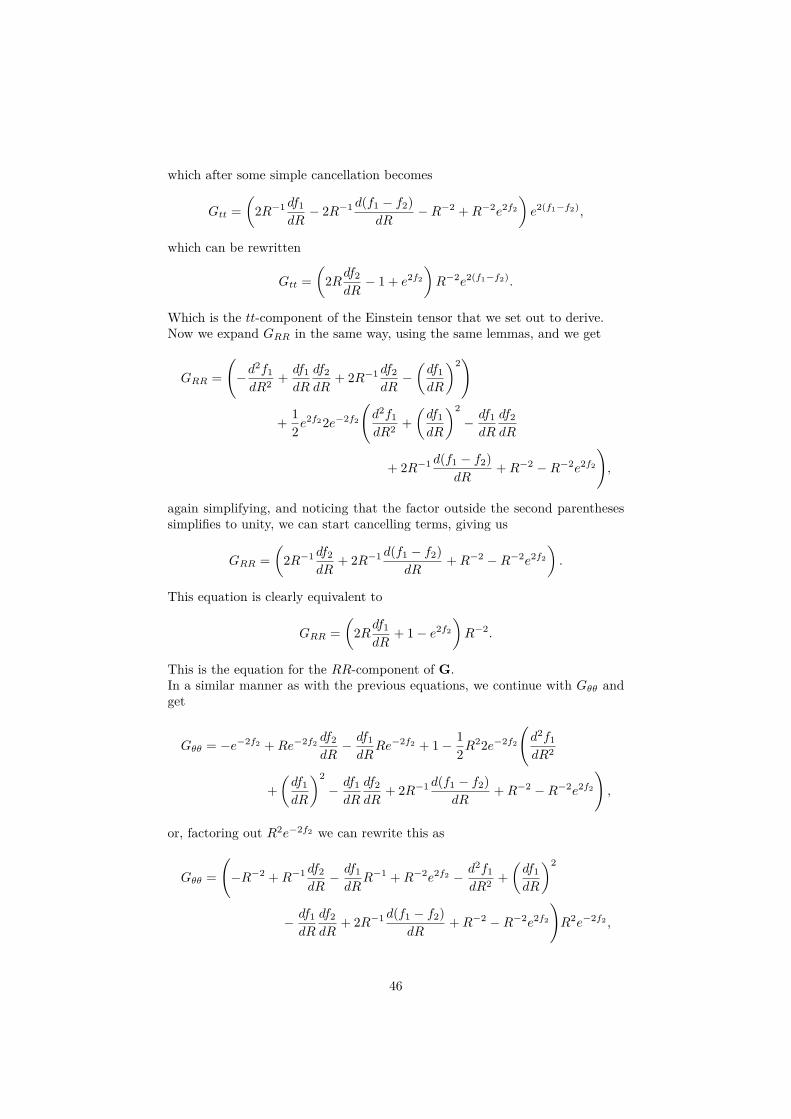
which after some simple cancellation becomes

Gtt =(

2R−1 df1

dR− 2R−1 d(f1 − f2)

dR−R−2 +R−2e2f2

)e2(f1−f2),

which can be rewritten

Gtt =(

2Rdf2

dR− 1 + e2f2

)R−2e2(f1−f2).

Which is the tt-component of the Einstein tensor that we set out to derive.Now we expand GRR in the same way, using the same lemmas, and we get

GRR =(−d

2f1

dR2 + df1

dR

df2

dR+ 2R−1 df2

dR−(df1

dR

)2)

+ 12e

2f22e−2f2

(d2f1

dR2 +(df1

dR

)2− df1

dR

df2

dR

+ 2R−1 d(f1 − f2)dR

+R−2 −R−2e2f2

),

again simplifying, and noticing that the factor outside the second parenthesessimplifies to unity, we can start cancelling terms, giving us

GRR =(

2R−1 df2

dR+ 2R−1 d(f1 − f2)

dR+R−2 −R−2e2f2

).

This equation is clearly equivalent to

GRR =(

2Rdf1

dR+ 1− e2f2

)R−2.

This is the equation for the RR-component of G.In a similar manner as with the previous equations, we continue with Gθθ andget

Gθθ = −e−2f2 +Re−2f2df2

dR− df1

dRRe−2f2 + 1− 1

2R22e−2f2

(d2f1

dR2

+(df1

dR

)2− df1

dR

df2

dR+ 2R−1 d(f1 − f2)

dR+R−2 −R−2e2f2

),

or, factoring out R2e−2f2 we can rewrite this as

Gθθ =(−R−2 +R−1 df2

dR− df1

dRR−1 +R−2e2f2 − d2f1

dR2 +(df1

dR

)2

− df1

dR

df2

dR+ 2R−1 d(f1 − f2)

dR+R−2 −R−2e2f2

)R2e−2f2 ,

46

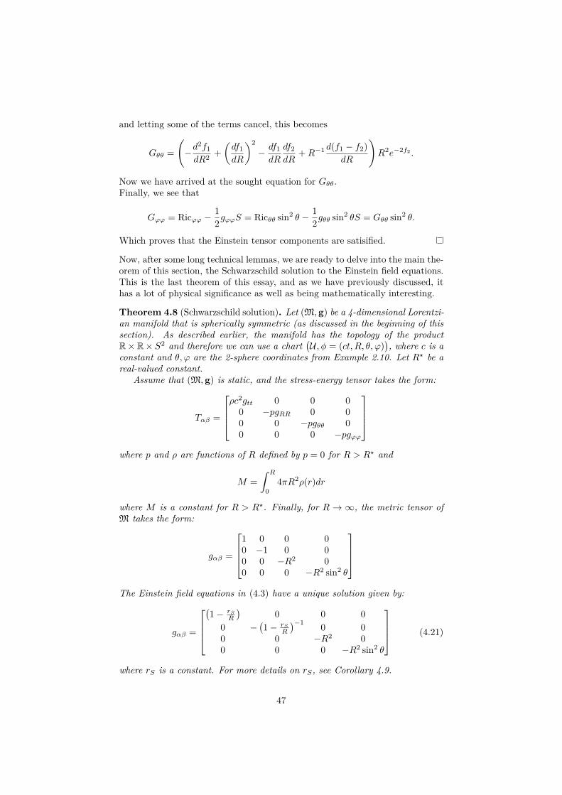
and letting some of the terms cancel, this becomes

Gθθ =(−d

2f1

dR2 +(df1

dR

)2− df1

dR

df2

dR+R−1 d(f1 − f2)

dR

)R2e−2f2 .

Now we have arrived at the sought equation for Gθθ.Finally, we see that

Gϕϕ = Ricϕϕ −12gϕϕS = Ricθθ sin2 θ − 1

2gθθ sin2 θS = Gθθ sin2 θ.

Which proves that the Einstein tensor components are satisified.

Now, after some long technical lemmas, we are ready to delve into the main the-orem of this section, the Schwarzschild solution to the Einstein field equations.This is the last theorem of this essay, and as we have previously discussed, ithas a lot of physical significance as well as being mathematically interesting.

Theorem 4.8 (Schwarzschild solution). Let (M,g) be a 4-dimensional Lorentzi-an manifold that is spherically symmetric (as discussed in the beginning of thissection). As described earlier, the manifold has the topology of the productR×R× S2 and therefore we can use a chart

(U , φ = (ct, R, θ, ϕ)

), where c is a

constant and θ, ϕ are the 2-sphere coordinates from Example 2.10. Let R? be areal-valued constant.

Assume that (M,g) is static, and the stress-energy tensor takes the form:

Tαβ =

ρc2gtt 0 0 0

0 −pgRR 0 00 0 −pgθθ 00 0 0 −pgϕϕ

where p and ρ are functions of R defined by p = 0 for R > R? and

M =∫ R

04πR2ρ(r)dr

where M is a constant for R > R?. Finally, for R → ∞, the metric tensor ofM takes the form:

gαβ =

1 0 0 00 −1 0 00 0 −R2 00 0 0 −R2 sin2 θ

The Einstein field equations in (4.3) have a unique solution given by:

gαβ =

(1− rS

R

)0 0 0

0 −(1− rS

R

)−1 0 00 0 −R2 00 0 0 −R2 sin2 θ

(4.21)

where rS is a constant. For more details on rS, see Corollary 4.9.

47

Proof. Inspired by the schematic proof in chapter 23 in [11], we prove thistheorem.

Using the coordinate system φ = (ct, R, θ, ϕ), we can deduce that due tospherical symmetry (which we have talked about earlier in this section), weneed only consider the following ansatz:

gαβ =

e2f1(R) 0 0 0

0 −e2f2(R) 0 00 0 −R2 00 0 0 −R2 sin2 θ

(4.22)

Since ∂t needs to be timelike everywhere and ∂R needs to be spacelike every-where, due to M being a Lorentzian manifold.

For some functions f1 : U → R and f2 : U → R. An exponential functionexists on every semi-Riemannian manifold (see, e.g. chapter 3 in [16]).Now from the definition of the Einstein field equations (4.3) we have that Gαβ =kTαβ . This and Lemma 4.7 gives us a set of four equations:

(2Rdf2

dR− 1 + e2f2

)R−2e2(f1−f2) = ke2f1ρc2, (4.23)(

2Rdf1

dR+ 1− e2f2

)R−2 = −ke2f2p, (4.24)(

−d2f1

dR2 +(df1

dR

)2− df1

dR

df2

dR+R−1 d(f1 − f2)

dR

)R2e−2f2 = −kR2p, (4.25)

Gθθ sin2 θ = −kR2 sin2 θp. (4.26)

We shall first solve the first of these first-order ordinary differential equations(4.23). First, we rewrite the equation as(

2Rdf2

dRe−2f2 − e−2f2 + 1

)R−2 = kρc2

and then this can be rewritten

d

dR

(R(1− e−2f2

))= kR2ρc2.

Now, by puttingrS = R−Re−2f2 ,

we obtain:

drSdR

= kR2ρc2,

and by integrating this becomes

rS(R) = kc2

4π

∫ R

04πR2ρdR,

48

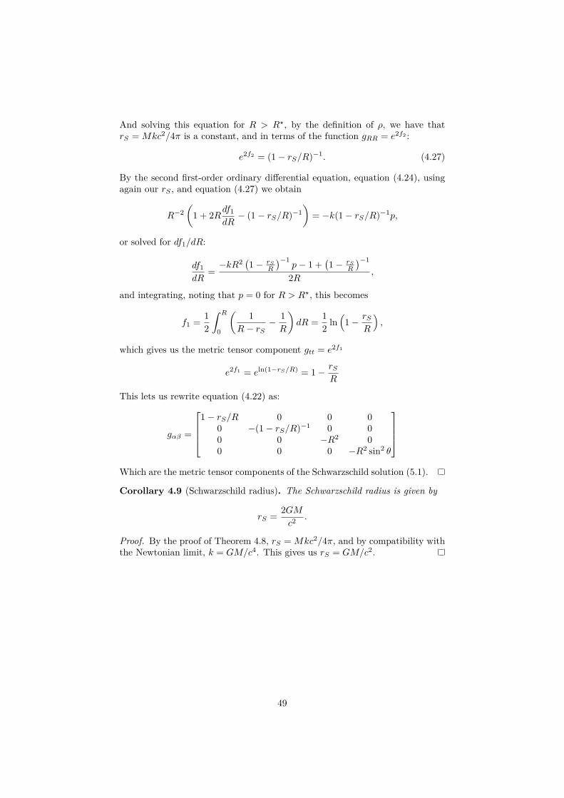
And solving this equation for R > R?, by the definition of ρ, we have thatrS = Mkc2/4π is a constant, and in terms of the function gRR = e2f2 :

e2f2 = (1− rS/R)−1. (4.27)

By the second first-order ordinary differential equation, equation (4.24), usingagain our rS , and equation (4.27) we obtain

R−2(

1 + 2Rdf1

dR− (1− rS/R)−1

)= −k(1− rS/R)−1p,

or solved for df1/dR:

df1

dR=−kR2 (1− rS

R

)−1p− 1 +

(1− rS

R

)−1

2R ,

and integrating, noting that p = 0 for R > R?, this becomes

f1 = 12

∫ R

0

(1

R− rS− 1R

)dR = 1

2 ln(

1− rSR

),

which gives us the metric tensor component gtt = e2f1

e2f1 = eln(1−rS/R) = 1− rSR

This lets us rewrite equation (4.22) as:

gαβ =

1− rS/R 0 0 0

0 −(1− rS/R)−1 0 00 0 −R2 00 0 0 −R2 sin2 θ

Which are the metric tensor components of the Schwarzschild solution (5.1).

Corollary 4.9 (Schwarzschild radius). The Schwarzschild radius is given by

rS = 2GMc2

.

Proof. By the proof of Theorem 4.8, rS = Mkc2/4π, and by compatibility withthe Newtonian limit, k = GM/c4. This gives us rS = GM/c2.

49

5 Applications to the Schwarzs-child solutionNow that we have familiarized ourselves with the Einstein field equations andthe Schwarzschild solution, we are ready to look at a few interesting examplesof applications. In particular, we shall in this chapter deal with geodesics onthe Schwarzschild manifold, as well as the Schwarzschild black hole.

From a physical perspective the geodesic paths correspond to the motionof particles in free fall. From a mathematical perspective, the spherical sym-metry of the Schwarzschild geometry leads to special classes of geodesics. TheSchwarzschild black hole, however, is a Schwarzschild manifold with rS > R?.

This may not appear to be much of a problem initially, but as we shall see, itleads to problems with the nondegeneracy of the metric tensor as R approachesrS .

5.1 The Schwarzschild manifoldThe Schwarzschild manifold is the 4-dimensional Lorentzian manifold M thathas a metric tensor

gαβ =

(1− rS

R

)0 0 0

0 −(1− rS

R

)−1 0 00 0 −R2 00 0 0 −R2 sin2 θ

(5.1)

where rS is the Schwarzschild radius from Corollary 4.9.This manifold (both the topology and the metric tensor) are used in the fol-

lowing sections on geodesics and singularities. This semi-Riemannian is calledthe Schwarzschild manifold, its metric tensor is called the Schwarzschild solu-tion, or Schwarzschild metric, since it is the unique solution to the Einstein fieldequations under the conditions of Theorem 4.8.

Often the line element (5.2) is referred to as the Schwarzschild metric, eventhough it is only related to it.

5.2 Schwarzschild geodesicsWe are interested in geodesics, because they are paths for particles in free fallabout the massive body. These paths are good approximations of the paths ofparticles around most celestial bodies, for example the orbit of the Moon aboutthe Earth, the path of a comet about the Sun or a satellite in orbit.

Remembering that these coordinates, for example the radius R, is not the ra-dius we would measure along some radial path. Rather, rewriting the Schwarzs-child solution in terms of the line element, we obtain (inspired by the similarderivation of geodesics in chapter 13 in [16]):

c2dτ2 =(

1− rSR

)c2dt2 − 1

1− rSR

dR2 −R2dθ2 −R2 sin2 θdϕ2, (5.2)

50

and this suggests that we would measure the proper length along a radialpath as

L =∫

(1− rS/R)−1/2dR.

Therefore we will derive the solutions to these curves and talk about the phys-ical properties of them. First off, we will assume that the path is initiallyequatorial, that is, θ(0) = π/2. Due to spherical symmetry, any geodesic can bereparametrized to be initially equatorial. We get four equations, but we startwith the three simple equations for ϕ, θ and t:

We will, on the Schwarzschild manifoldM, use the Schwarzschild coordinatesφ = (ct, R, θ, ϕ). These coordinates are orthogonal, and so we can use thegeodesic equations derived in Example 2.23.

ddτ

((1− rS

R

)c2 dtdτ

)= 1

2∑α ∂tgαα

(duα

dτ

)2 = 0,ddτ

(R2 sin2 θ dϕdτ

)= 1

2∑α ∂ϕgαα

(duα

dτ

)2 = 0,ddτ

(R2 dθ

dτ

)= sin θ cos θ

(dϕdτ

)2,

and expanding the two first equations, we find constants for the energy1 andangular momentum of the particle. Calling the energy pt and the angular mo-mentum pϕ, we obtain: (

1− rSR

) dtdτ

= pt,

R2 dϕ

dτ= pϕ,

θ = π/2.

From the line element (5.2), we get an energy equation (remembering θ = π/2):

c2 =(

1− rSR

)c2(dt

dτ

)2− 1

1− rSR

(dR

dτ

)2−R2

(dϕ

dτ

)2,

and therefore (dR

dτ

)2= c2p2

t −(1− rS

R

)p2ϕ

R2 + c2rSR− c2. (5.3)

Now we can see the last three terms on the right-hand side as a sort of potentialenergy of the particle. In fact, let us call this function

U(R) = c2 − c2 rSR

+p2ϕ

R2 −p2ϕrS

R3 .

We may notice that there are terms proportional to 1/R3, which we would notexpect from the Newtonian gravitation.

This equation (5.3) holds a lot of physical significance. We have the extraterm 1/R3 in the potential, and we have the relationship between the potentialenergy, the energy and the radial velocity,(

dR

dτ

)2= c2p2

t − U. (5.4)

1In fact, the energy at infinity per unit mass.

51

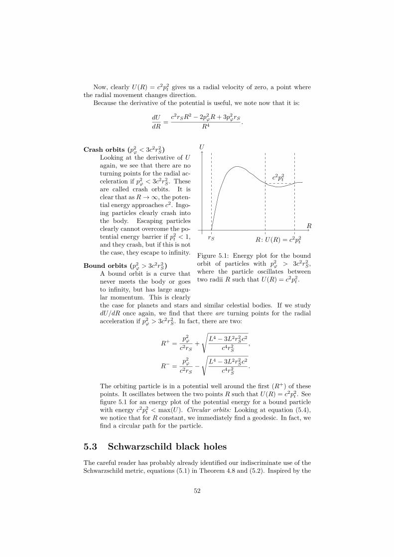
Now, clearly U(R) = c2p2t gives us a radial velocity of zero, a point where

the radial movement changes direction.Because the derivative of the potential is useful, we note now that it is:

dU

dR=c2rSR

2 − 2p2ϕR+ 3p2

ϕrS

R4 .

R

U

rS

c2p2t

R : U(R) = c2p2t

Figure 5.1: Energy plot for the boundorbit of particles with p2

ϕ > 3c2r2S ,

where the particle oscillates betweentwo radii R such that U(R) = c2p2

t .

Crash orbits (p2ϕ < 3c2r2

S)Looking at the derivative of Uagain, we see that there are noturning points for the radial ac-celeration if p2

ϕ < 3c2r2S . These

are called crash orbits. It isclear that asR→∞, the poten-tial energy approaches c2. Ingo-ing particles clearly crash intothe body. Escaping particlesclearly cannot overcome the po-tential energy barrier if p2

t < 1,and they crash, but if this is notthe case, they escape to infinity.

Bound orbits (p2ϕ > 3c2r2

S)A bound orbit is a curve thatnever meets the body or goesto infinity, but has large angu-lar momentum. This is clearlythe case for planets and stars and similar celestial bodies. If we studydU/dR once again, we find that there are turning points for the radialacceleration if p2

ϕ > 3c2r2S . In fact, there are two:

R+ =p2ϕ

c2rS+

√L4 − 3L2r2

Sc2

c4r2S

,

R− =p2ϕ

c2rS−

√L4 − 3L2r2

Sc2

c4r2S

.

The orbiting particle is in a potential well around the first (R+) of thesepoints. It oscillates between the two points R such that U(R) = c2p2

t . Seefigure 5.1 for an energy plot of the potential energy for a bound particlewith energy c2p2

t < max(U). Circular orbits: Looking at equation (5.4),we notice that for R constant, we immediately find a geodesic. In fact, wefind a circular path for the particle.

5.3 Schwarzschild black holesThe careful reader has probably already identified our indiscriminate use of theSchwarzschild metric, equations (5.1) in Theorem 4.8 and (5.2). Inspired by the

52

discussions of Schwarzschild black holes in [11] and [16], we try to explain theseproblems. First, it is clear that R = 0 is not allowed. However, this is trivialand does not in fact change anything.

Second, we run into trouble when trying to move at R < R?, where R? isthe boundary of the body in question. However, this is rarely a problem. Third,however, we notice that at R = rS the line element breaks down.

This leads us to break the manifold M into two regions:

MB = R× R : R < rS × S2 and ME = R× R : rS < R <∞× S2.

Normally, for a star R? > rS , and we only work with the Schwarzschildexterior spacetime ME , and everything in this chapter so far needs no furthermathematical motivation.

However, if we look at an object with R? < rS , it is a black hole. In fact,if R? < rS , then R? = 0, and the mass becomes a point mass, a gravitationalsingularity. Most of the time, we handle the black hole by ignoring this discon-tinuity, and using M = ME ∪MB .

That is not to say that we do not find the geometrical properties of the blackhole interesting.

Looking at the motion of a particle towards a black hole, we notice that thetime dilation dt = dτ/(1− rS/R)1/2 →∞ as R→ rS . This means that it is notphysically possible to observe a particle entering a black hole, while of course itdoes not take infinite time in the reference frame of the particle itself.

Furthermore, for R < rS , it is clear that 1−rS/R is negative, and t becomesa spacelike coordinate while R becomes the timelike coordinate.

53

Bibliography[1] Einstein, Albert (1905). Zur Elektrodynamik bewegter Körper, Annalen der

Physik 17: 891.

[2] Einstein, Albert (1915). Die Feldgleichungen der Gravitation. Sitzungs-berichte der Preussischen Akademie der Wissenschaften zu Berlin: 844-847.

[3] Einstein, Albert (1916). Die Grundlage der allgemeinen RelativitätstheorieAnnalen der Physik 49.

[4] Foster, James & Nightingale, J. David (2006). A Short Course in GeneralRelativity. 3rd Edition. New York: Springer.

[5] Kerr, Roy (1963). Gravitational field of a spinning mass as an example ofalgebraically special metrics. Physical Review Letters 11 (5): 237-238.

[6] Kippenhahn, Rudolf (1983). 100 Billion Suns: The Birth, Life, and Deathof the Stars. Princeton: Princeton University Press.

[7] Lee, Jeffrey M. (2009). Manifolds and Differential Geometry. Providence:American Mathematical Society.

[8] Lee, John M. (1997). Riemannian Manifolds. New York: Springer.

[9] Martin, Daniel (2002). Manifold Theory: Introduction for MathematicalPhysicists. West Sussex: Horwood Publishing Limited.

[10] Minkowski, Hermann (1908/9). Raum und Zeit. Jahresberichte derDeutschen Mathematiker-Vereinigung : 75− 88.

[11] Misner, Charles W.; Thorne, Kip S. & Wheeler, John A. (1973). Gravita-tion. San Fransisco: W. H. Freeman and Company.

[12] Moffat, John W. (1994). Nonsymmetric Gravitational Theory. Journal ofMathematical Physics. 36 (7): 3722-3732.

[13] Müller, Olaf & Sánchez, Miguel (2011). Lorentzian manifolds isometricallyembeddable in LN . Transactions of the American Mathematical Society 363(10): 5367-5379.

[14] Nash, John (1956). The imbedding problem for Riemannian manifolds. An-nals of Mathematics 63 (1) : 20− 63.

[15] Newman, Ezra; Couch, E.; Chinnapared, K.; Exton, A.; Prakash, A.; &Torrence, R. J. (1965).Metric of a Rotating, Charged Mass. Journal of Math-ematical Physics 6 (6) : 918− 919.

[16] O’Neill, Barett (1983). Semi-Riemannian Geometry. London: AcademicPress.

[17] Riemann, Bernhard; translated by Clifford, William (1868). On the Hy-potheses which lie at the Bases of Geometry. Nature 8 1873 14-17, 36, 37.

54

[18] Royden, Halsey L. (1988) Real Analysis. 3rd Edition. New York: MacmillanPublishing Company.

[19] Schwarzschild, Karl (1916). Über das Gravitationsfeld eines Massen-punktes nach der Einsteinschen Theorie. Sitzungsberichte der Königlich-Preussischen Akademie der Wissenschaften.

[20] Teschl, Gerald (2012). Ordinary Differential Equations and Dynamical Sys-tems. Providence: American Mathematical Society.

[21] Tu, Loring W. (2011). An Introduction to Manifolds. 2nd Edition. NewYork: Springer.

[22] Whitney, Hassler (1936). Differentiable Manifolds. Annals of Mathematics37 (3) : 645− 680.

55