1

The Sam Loyd 15-Puzzle

Richard Hayes

June 2001

Abstract

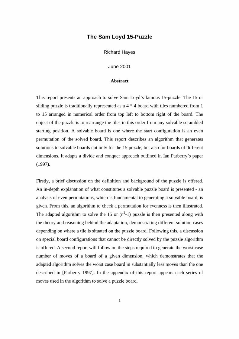
This report presents an approach to solve Sam Loyd’s famous 15-puzzle. The 15 or

sliding puzzle is traditionally represented as a 4 * 4 board with tiles numbered from 1

to 15 arranged in numerical order from top left to bottom right of the board. The

object of the puzzle is to rearrange the tiles in this order from any solvable scrambled

starting position. A solvable board is one where the start configuration is an even

permutation of the solved board. This report describes an algorithm that generates

solutions to solvable boards not only for the 15 puzzle, but also for boards of different

dimensions. It adapts a divide and conquer approach outlined in Ian Parberry’s paper

(1997).

Firstly, a brief discussion on the definition and background of the puzzle is offered.

An in-depth explanation of what constitutes a solvable puzzle board is presented - an

analysis of even permutations, which is fundamental to generating a solvable board, is

given. From this, an algorithm to check a permutation for evenness is then illustrated.

The adapted algorithm to solve the 15 or (n2-1) puzzle is then presented along with

the theory and reasoning behind the adaptation, demonstrating different solution cases

depending on where a tile is situated on the puzzle board. Following this, a discussion

on special board configurations that cannot be directly solved by the puzzle algorithm

is offered. A second report will follow on the steps required to generate the worst case

number of moves of a board of a given dimension, which demonstrates that the

adapted algorithm solves the worst case board in substantially less moves than the one

described in [Parberry 1997]. In the appendix of this report appears each series of

moves used in the algorithm to solve a puzzle board.

2

1 The (n2-1) Puzzle

1.1 Introduction

The (n2-1) puzzle is traditionally represented as a 4 * 4 board with tiles numbered

from 1 to 15 arranged in numerical order from top left to bottom right of the board

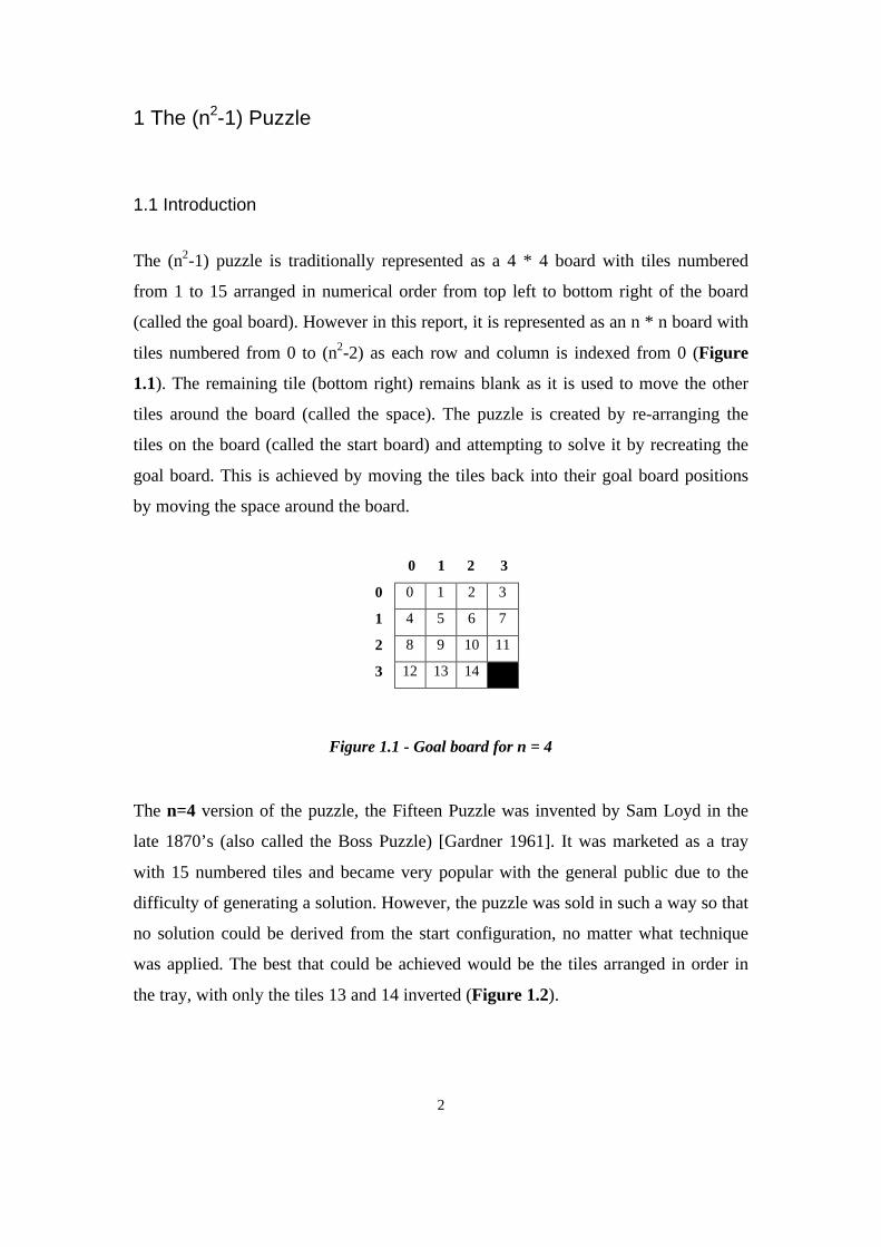
(called the goal board). However in this report, it is represented as an n * n board with

tiles numbered from 0 to (n2-2) as each row and column is indexed from 0 (Figure

1.1). The remaining tile (bottom right) remains blank as it is used to move the other

tiles around the board (called the space). The puzzle is created by re-arranging the

tiles on the board (called the start board) and attempting to solve it by recreating the

goal board. This is achieved by moving the tiles back into their goal board positions

by moving the space around the board.

0 1 2 3

0 0 1 2 3

1 4 5 6 7

2 8 9 10 11

3 12 13 14

Figure 1.1 - Goal board for n = 4

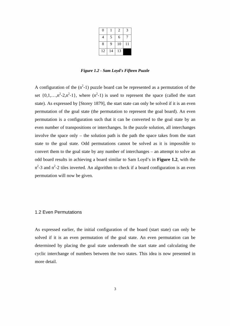
The n=4 version of the puzzle, the Fifteen Puzzle was invented by Sam Loyd in the

late 1870’s (also called the Boss Puzzle) [Gardner 1961]. It was marketed as a tray

with 15 numbered tiles and became very popular with the general public due to the

difficulty of generating a solution. However, the puzzle was sold in such a way so that

no solution could be derived from the start configuration, no matter what technique

was applied. The best that could be achieved would be the tiles arranged in order in

the tray, with only the tiles 13 and 14 inverted (Figure 1.2).

3

0 1 2 3

4 5 6 7

8 9 10 11

12 14 13

Figure 1.2 - Sam Loyd's Fifteen Puzzle

A configuration of the (n2-1) puzzle board can be represented as a permutation of the

set {0,1,…,n2-2,n2-1}, where (n2-1) is used to represent the space (called the start

state). As expressed by [Storey 1879], the start state can only be solved if it is an even

permutation of the goal state (the permutation to represent the goal board). An even

permutation is a configuration such that it can be converted to the goal state by an

even number of transpositions or interchanges. In the puzzle solution, all interchanges

involve the space only – the solution path is the path the space takes from the start

state to the goal state. Odd permutations cannot be solved as it is impossible to

convert them to the goal state by any number of interchanges – an attempt to solve an

odd board results in achieving a board similar to Sam Loyd’s in Figure 1.2, with the

n2-3 and n2-2 tiles inverted. An algorithm to check if a board configuration is an even

permutation will now be given.

1.2 Even Permutations

As expressed earlier, the initial configuration of the board (start state) can only be

solved if it is an even permutation of the goal state. An even permutation can be

determined by placing the goal state underneath the start state and calculating the

cyclic interchange of numbers between the two states. This idea is now presented in

more detail.

4

1.2.1 Determining a state's evenness

There are two cases to consider when determining whether a start state is even or not:

1/ The number n2-1 (space) is the final element in the start state i.e. already in the

same position as it is in the goal state.

2/ The number n2-1 is not the final element in the start state.

1.2.1.1 Space in its default position

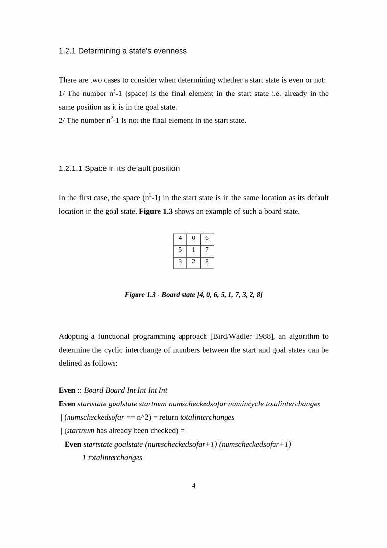
In the first case, the space (n2-1) in the start state is in the same location as its default

location in the goal state. Figure 1.3 shows an example of such a board state.

4 0 6

5 1 7

3 2 8

Figure 1.3 - Board state [4, 0, 6, 5, 1, 7, 3, 2, 8]

Adopting a functional programming approach [Bird/Wadler 1988], an algorithm to

determine the cyclic interchange of numbers between the start and goal states can be

defined as follows:

Even :: Board Board Int Int Int Int

Even startstate goalstate startnum numscheckedsofar numincycle totalinterchanges

| (numscheckedsofar == n^2) = return totalinterchanges

| (startnum has already been checked) =

Even startstate goalstate (numscheckedsofar+1) (numscheckedsofar+1)

1 totalinterchanges

5

| otherwise =

check number in startnum's startstate location in goalstate (called goalnum),

if (goalnum == numscheckedsofar)

then

Even startstate goalstate (numscheckedsofar + 1) (numscheckedsofar + 1)

1 (totalinterchanges+numincycle-1)

else

Even startstate goalstate goalnum numscheckedsofar (numincycle+1)

totalinterchanges

startnum represents the current number in a cycle being checked, numscheckedsofar

represents the current number in startstate being checked, numincycle keeps a track of

how many numbers have appeared in a cycle, while totalinterchanges is the total

number of cyclic interchanges between the two states.

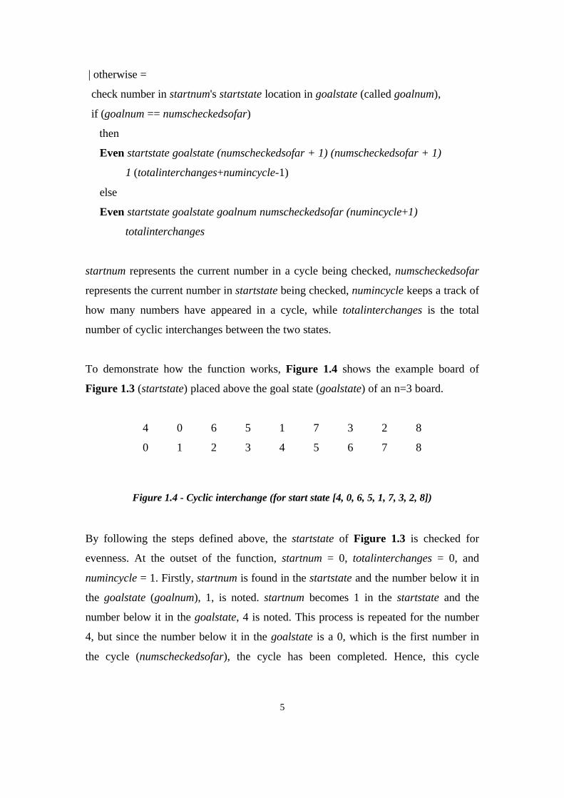
To demonstrate how the function works, Figure 1.4 shows the example board of

Figure 1.3 (startstate) placed above the goal state (goalstate) of an n=3 board.

4 0 6 5 1 7 3 2 8

0 1 2 3 4 5 6 7 8

Figure 1.4 - Cyclic interchange (for start state [4, 0, 6, 5, 1, 7, 3, 2, 8])

By following the steps defined above, the startstate of Figure 1.3 is checked for

evenness. At the outset of the function, startnum = 0, totalinterchanges = 0, and

numincycle = 1. Firstly, startnum is found in the startstate and the number below it in

the goalstate (goalnum), 1, is noted. startnum becomes 1 in the startstate and the

number below it in the goalstate, 4 is noted. This process is repeated for the number

4, but since the number below it in the goalstate is a 0, which is the first number in

the cycle (numscheckedsofar), the cycle has been completed. Hence, this cycle

6

consists of the following numbers: 0,1,4,0 - the number of total cyclic interchanges so

far (totalinterchanges) is (numincycle - 1) = 2.

The next number to be found is 1, but since it has already appeared in a cycle, there is

no need to check it. 2 is then checked, and the following cycle is detected: 2,7,5,3,6,2.

This process is repeated for the remaining numbers 3 to 8, the number denoting the

space. As a result, the following cycles are detected (Figure 1.5):

(0 1 4) (2 7 5 3 6) (8)

Figure 1.5 - Cycles for start state [4, 0, 6, 5, 1, 7, 3, 2, 8]

Hence, the first cycle contains 3 numbers i.e. 2 interchanges, the second cycle

contains 5 numbers i.e. 4 interchanges and the third cycle contains 1 number i.e. no

interchanges. By adding the total number of interchanges, it is found that there are a

total of 6 interchanges in the start state. Since 6 is an even number, it can be deduced

that the start state [4, 0, 6, 5, 1, 7, 3, 2, 8] is even and therefore a path from this state

to the goal state [0, 1, 2, 3, 4, 5, 6, 7, 8] can be determined.

By applying this method to all board states of the numbers 0, 1,.., n2-1, it can be

shown that there are 2

)!1( 2 −n even permutations when n2-1 is in the same position in the

start and goal state.

1.2.1.2 Space not in its default position

The first case takes into consideration only those start states with the space in its

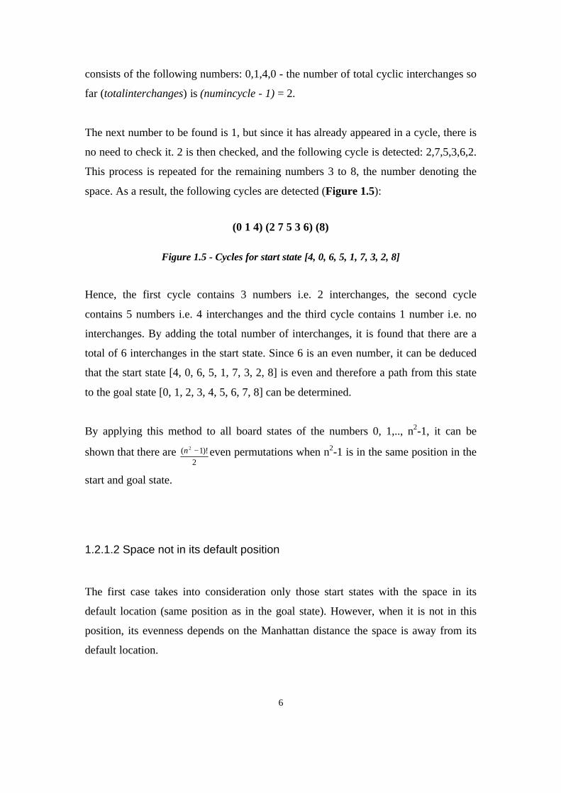
default location (same position as in the goal state). However, when it is not in this

position, its evenness depends on the Manhattan distance the space is away from its

default location.

7

0 1 4

8 6 7

5 2 3

Figure 1.6 - Board state [0, 1, 4, 8, 6, 7, 5, 2, 3]

As defined in [Parberry 1997], the Manhattan distance of a number is the minimum

amount of moves needed to move that number into its position in the goal state. By

adding the number of moves required to move the space (n2-1) into its default location

to the number of interchanges in the start state, it can be determined if this state is odd

or even.

Once again, the start state is placed underneath the goal state. However as seen above,

this time n2-1 (8) is not in its default location.

0 1 4 8 6 7 5 2 3

0 1 2 3 4 5 6 7 8

Figure 1.7 - Cyclic interchange (for start state [0, 1, 4, 8, 6, 7, 5, 2, 3])

By following the algorithm presented in 1.2.1.1 for when n2-1 is in its default

location, the following cycles can be detected:

(0) (1) (2 7 5 6 4) (3 8)

Figure 1.8 - Cycles for start state [0, 1, 4, 8, 6, 7, 5, 2, 3]

The first and second cycles contain 1 number i.e. no interchanges, the third cycle

contains 5 numbers i.e. 4 interchanges and the fourth cycle contains 2 numbers i.e. 1

interchange. By adding the total number of interchanges, in this case there is a total

number of 5 interchanges in this start state. Since 5 is an odd number, it would seem

that the permutation [0, 1, 4, 8, 6, 7, 5, 2, 3] is odd and therefore cannot be solved.

8

However, since n2-1 (8) is not in its default location, it has to be ascertained how

many moves are needed to move it into its goal location.

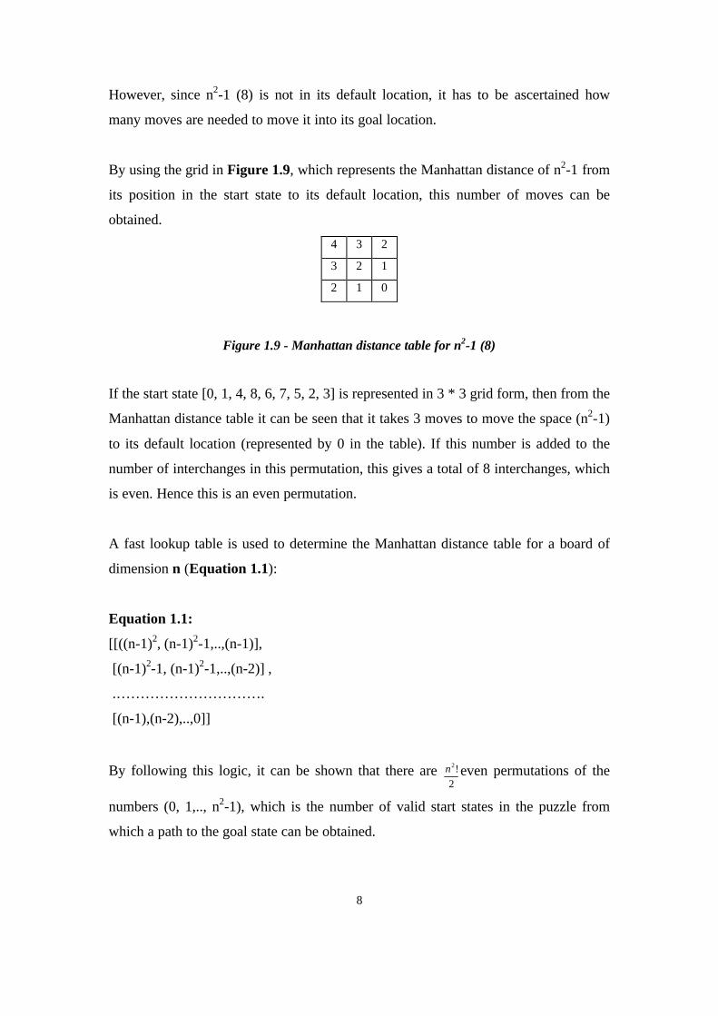
By using the grid in Figure 1.9, which represents the Manhattan distance of n2-1 from

its position in the start state to its default location, this number of moves can be

obtained.

4 3 2

3 2 1

2 1 0

Figure 1.9 - Manhattan distance table for n2-1 (8)

If the start state [0, 1, 4, 8, 6, 7, 5, 2, 3] is represented in 3 * 3 grid form, then from the

Manhattan distance table it can be seen that it takes 3 moves to move the space (n2-1)

to its default location (represented by 0 in the table). If this number is added to the

number of interchanges in this permutation, this gives a total of 8 interchanges, which

is even. Hence this is an even permutation.

A fast lookup table is used to determine the Manhattan distance table for a board of

dimension n (Equation 1.1):

Equation 1.1:

[[((n-1)2, (n-1)2-1,..,(n-1)],

[(n-1)2-1, (n-1)2-1,..,(n-2)] ,

.………………………….

[(n-1),(n-2),..,0]]

By following this logic, it can be shown that there are 2

!2n even permutations of the

numbers (0, 1,.., n2-1), which is the number of valid start states in the puzzle from

which a path to the goal state can be obtained.

9

2 (n2-1) Puzzle Algorithm

2.1 Introduction

The high-level algorithm to solve the (n2-1) puzzle from any even configuration of an

n * n board is based on the one outlined in [Parberry 1997]. In his paper, Parberry

outlines a divide and conquer algorithm which repeatedly reduces the n * n puzzle

into an (n-1) * (n-1) puzzle, thus placing the first (n-3) rows and columns into

position, until the puzzle is reduced to the base case 3 * 3 board which is solved by

brute force [Schofield 1967].

The algorithm presented here also repeatedly reduces the n * n puzzle into an (n-1) *

(n-1) puzzle, but places the first (n-1) rows and columns into place, thus reducing the

puzzle to a base case of n=1, hence solving the puzzle without treating any row or

column in a special way. It defines a specific set of moves that tries to guarantee the

shortest path a tile can take in order to move it home using this method. It also lets the

user solve a board for n ≥ 2, unlike Parberry’s which can only solve for n ≥ 3.

2.2 Algorithm

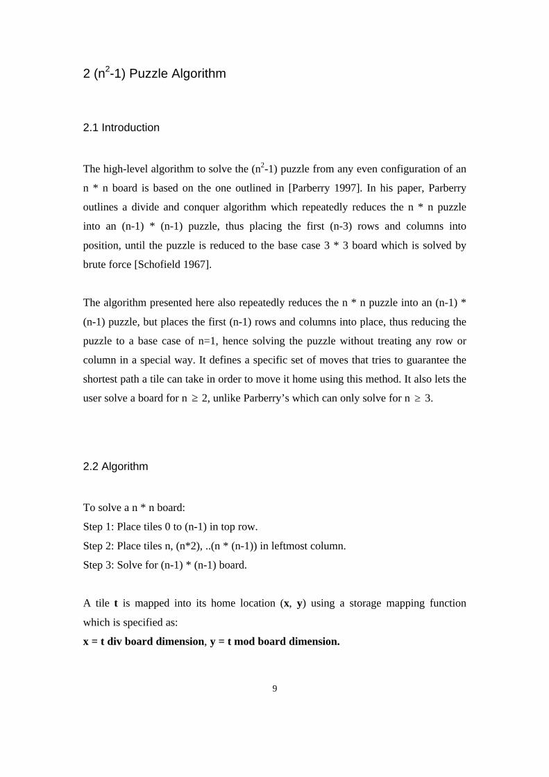
To solve a n * n board:

Step 1: Place tiles 0 to (n-1) in top row.

Step 2: Place tiles n, (n*2), ..(n * (n-1)) in leftmost column.

Step 3: Solve for (n-1) * (n-1) board.

A tile t is mapped into its home location (x, y) using a storage mapping function

which is specified as:

x = t div board dimension, y = t mod board dimension.

10

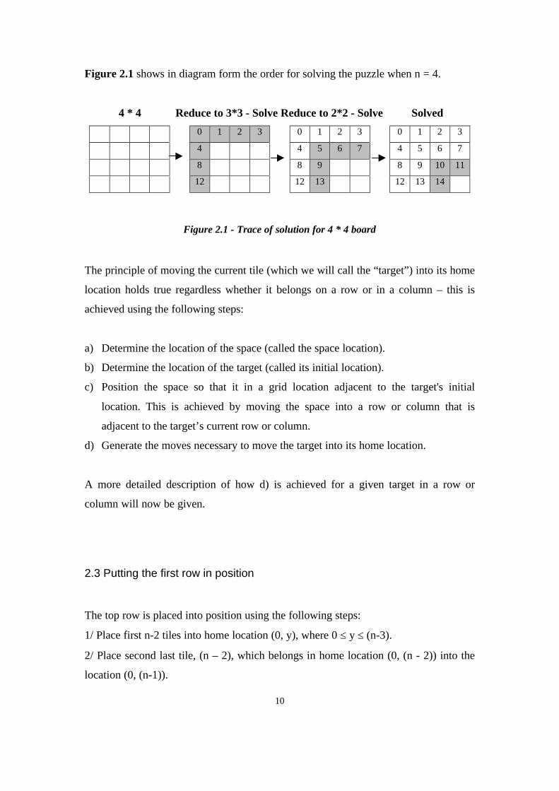
Figure 2.1 shows in diagram form the order for solving the puzzle when n = 4.

4 * 4 Reduce to 3*3 - Solve Reduce to 2*2 - Solve Solved

0 1 2 3 0 1 2 3 0 1 2 3

4 4 5 6 7 4 5 6 7

8 8 9 8 9 10 11

12 12 13 12 13 14

Figure 2.1 - Trace of solution for 4 * 4 board

The principle of moving the current tile (which we will call the “target”) into its home

location holds true regardless whether it belongs on a row or in a column – this is

achieved using the following steps:

a) Determine the location of the space (called the space location).

b) Determine the location of the target (called its initial location).

c) Position the space so that it in a grid location adjacent to the target's initial

location. This is achieved by moving the space into a row or column that is

adjacent to the target’s current row or column.

d) Generate the moves necessary to move the target into its home location.

A more detailed description of how d) is achieved for a given target in a row or

column will now be given.

2.3 Putting the first row in position

The top row is placed into position using the following steps:

1/ Place first n-2 tiles into home location (0, y), where 0 ≤ y ≤ (n-3).

2/ Place second last tile, (n – 2), which belongs in home location (0, (n - 2)) into the

location (0, (n-1)).

11

3/ Place last tile, (n-1), which belongs in home location (0, (n-1)), below tile (n-2) into

the location (1, (n-1)).

4/ Complete row by moving these two tiles into their home locations by a predefined

series of moves.

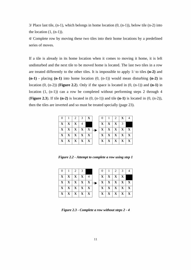
If a tile is already in its home location when it comes to moving it home, it is left

undisturbed and the next tile to be moved home is located. The last two tiles in a row

are treated differently to the other tiles. It is impossible to apply 1/ to tiles (n-2) and

(n-1) - placing (n-1) into home location (0, (n-1)) would mean disturbing (n-2) in

location (0, (n-2)) (Figure 2.2). Only if the space is located in (0, (n-1)) and (n-1) in

location (1, (n-1)) can a row be completed without performing steps 2 through 4

(Figure 2.3). If tile (n-2) is located in (0, (n-1)) and tile (n-1) is located in (0, (n-2)),

then the tiles are inverted and so must be treated specially (page 23).

0 1 2 3 X 0 1 2 X 4

X X X 4 X X X 3

X X X X X X X X X X

X X X X X X X X X X

X X X X X X X X X X

Figure 2.2 - Attempt to complete a row using step 1

0 1 2 3 0 1 2 3 4

X X X X 4 X X X X

X X X X X X X X X X

X X X X X X X X X X

X X X X X X X X X X

Figure 2.3 - Complete a row without steps 2 - 4

12

2.3.1 Placing the first (n-2) tiles in a row

Depending on the column in which the target initially resides in, the target will either

be to the left, to the right or in the same column as its home location (called its home

column). These cases will now be treated in detail.

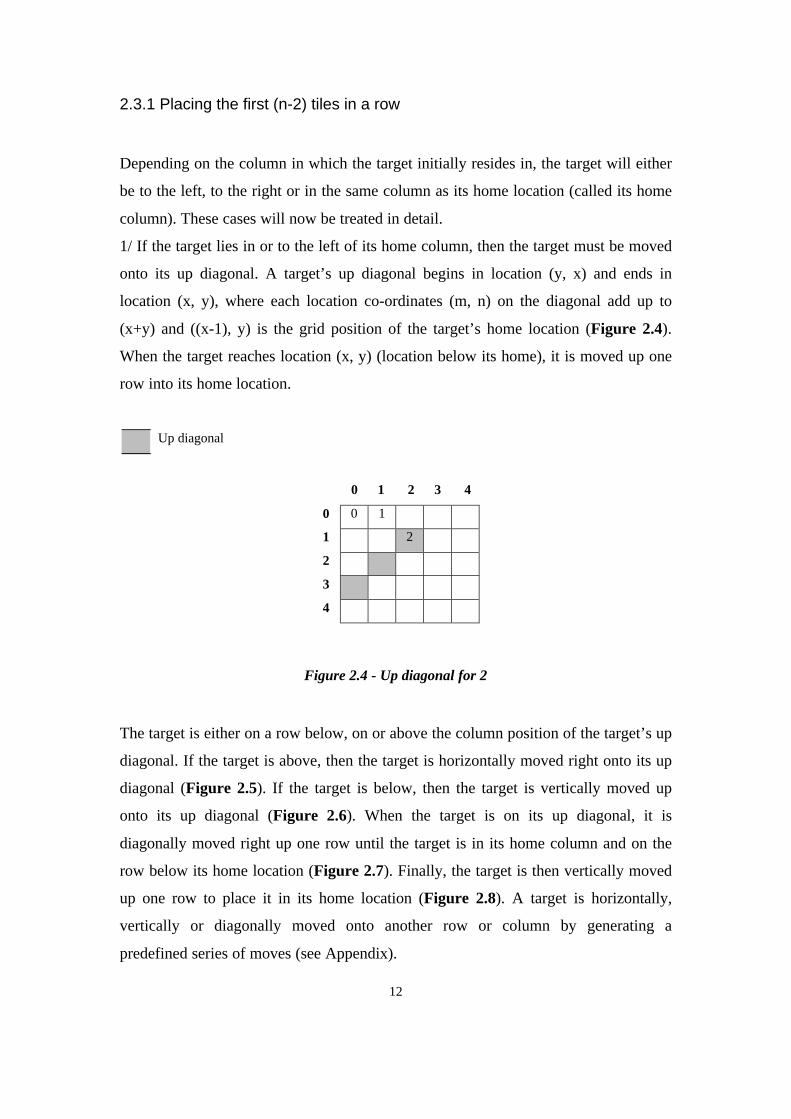
1/ If the target lies in or to the left of its home column, then the target must be moved

onto its up diagonal. A target’s up diagonal begins in location (y, x) and ends in

location (x, y), where each location co-ordinates (m, n) on the diagonal add up to

(x+y) and ((x-1), y) is the grid position of the target’s home location (Figure 2.4).

When the target reaches location (x, y) (location below its home), it is moved up one

row into its home location.

Up diagonal

0 1 2 3 4

0 0 1

1 2

2

3

4

Figure 2.4 - Up diagonal for 2

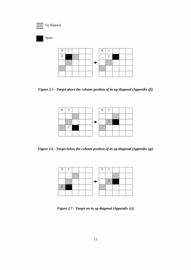
The target is either on a row below, on or above the column position of the target’s up

diagonal. If the target is above, then the target is horizontally moved right onto its up

diagonal (Figure 2.5). If the target is below, then the target is vertically moved up

onto its up diagonal (Figure 2.6). When the target is on its up diagonal, it is

diagonally moved right up one row until the target is in its home column and on the

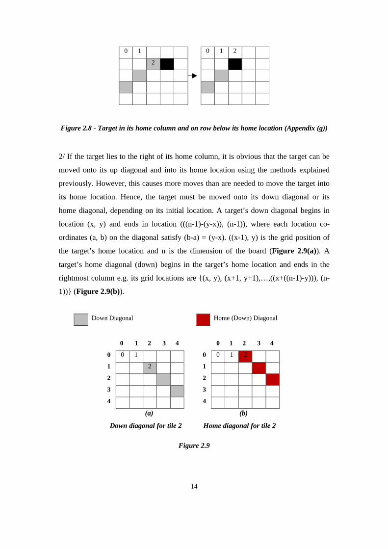
row below its home location (Figure 2.7). Finally, the target is then vertically moved

up one row to place it in its home location (Figure 2.8). A target is horizontally,

vertically or diagonally moved onto another row or column by generating a

predefined series of moves (see Appendix).

13

Up diagonal

Space

0 1 0 1

2 2

Figure 2.5 - Target above the column position of its up diagonal (Appendix (f))

0 1 0 1

2

2

Figure 2.6 - Target below the column position of its up diagonal (Appendix (g))

0 1 0 1

2

2

Figure 2.7 - Target on its up diagonal (Appendix (c))

14

0 1 0 1 2

2

Figure 2.8 - Target in its home column and on row below its home location (Appendix (g))

2/ If the target lies to the right of its home column, it is obvious that the target can be

moved onto its up diagonal and into its home location using the methods explained

previously. However, this causes more moves than are needed to move the target into

its home location. Hence, the target must be moved onto its down diagonal or its

home diagonal, depending on its initial location. A target’s down diagonal begins in

location (x, y) and ends in location (((n-1)-(y-x)), (n-1)), where each location co-

ordinates (a, b) on the diagonal satisfy (b-a) = (y-x). ((x-1), y) is the grid position of

the target’s home location and n is the dimension of the board (Figure 2.9(a)). A

target’s home diagonal (down) begins in the target’s home location and ends in the

rightmost column e.g. its grid locations are {(x, y), (x+1, y+1),…,((x+((n-1)-y))), (n-

1))} (Figure 2.9(b)).

Down Diagonal Home (Down) Diagonal

0 1 2 3 4 0 1 2 3 4

0 0 1 0 0 1 2

1 2 1

2 2

3 3

4 4

(a) (b)

Down diagonal for tile 2 Home diagonal for tile 2

Figure 2.9

15

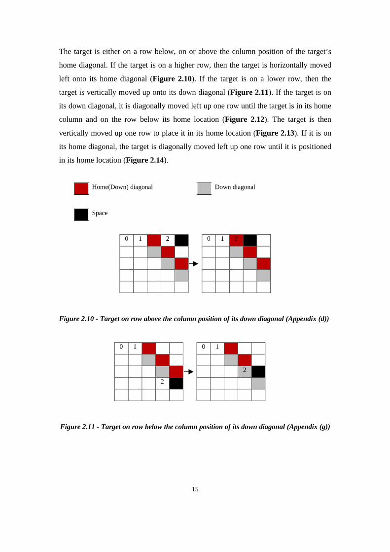
The target is either on a row below, on or above the column position of the target’s

home diagonal. If the target is on a higher row, then the target is horizontally moved

left onto its home diagonal (Figure 2.10). If the target is on a lower row, then the

target is vertically moved up onto its down diagonal (Figure 2.11). If the target is on

its down diagonal, it is diagonally moved left up one row until the target is in its home

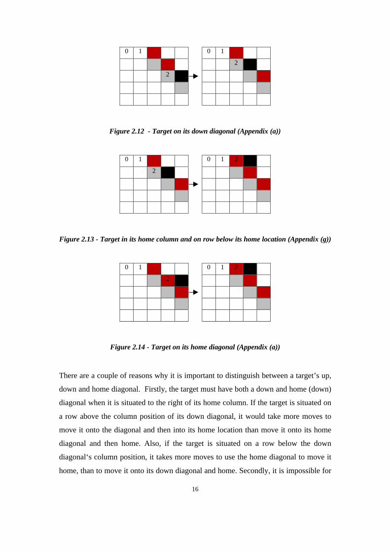
column and on the row below its home location (Figure 2.12). The target is then

vertically moved up one row to place it in its home location (Figure 2.13). If it is on

its home diagonal, the target is diagonally moved left up one row until it is positioned

in its home location (Figure 2.14).

Home(Down) diagonal Down diagonal

Space

0 1 2 0 1 2

Figure 2.10 - Target on row above the column position of its down diagonal (Appendix (d))

0 1 0 1

2

2

Figure 2.11 - Target on row below the column position of its down diagonal (Appendix (g))

16

0 1 0 1

2

2

Figure 2.12 - Target on its down diagonal (Appendix (a))

0 1 0 1 2

2

Figure 2.13 - Target in its home column and on row below its home location (Appendix (g))

0 1 0 1 2

2

Figure 2.14 - Target on its home diagonal (Appendix (a))

There are a couple of reasons why it is important to distinguish between a target’s up,

down and home diagonal. Firstly, the target must have both a down and home (down)

diagonal when it is situated to the right of its home column. If the target is situated on

a row above the column position of its down diagonal, it would take more moves to

move it onto the diagonal and then into its home location than move it onto its home

diagonal and then home. Also, if the target is situated on a row below the down

diagonal‘s column position, it takes more moves to use the home diagonal to move it

home, than to move it onto its down diagonal and home. Secondly, it is impossible for

17

the target to have a home (up) diagonal when it lies to the left or is in its home

column. If a target was to be moved onto its home (up) diagonal, it would dislodge

tiles already placed in their home locations.

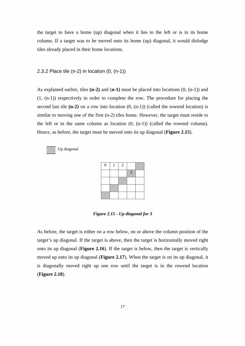
2.3.2 Place tile (n-2) in location (0, (n-1))

As explained earlier, tiles (n-2) and (n-1) must be placed into locations (0, (n-1)) and

(1, (n-1)) respectively in order to complete the row. The procedure for placing the

second last tile (n-2) on a row into location (0, (n-1)) (called the rowend location) is

similar to moving one of the first (n-2) tiles home. However, the target must reside to

the left or in the same column as location (0, (n-1)) (called the rowend column).

Hence, as before, the target must be moved onto its up diagonal (Figure 2.15).

Up diagonal

0 1 2

3

Figure 2.15 - Up diagonal for 3

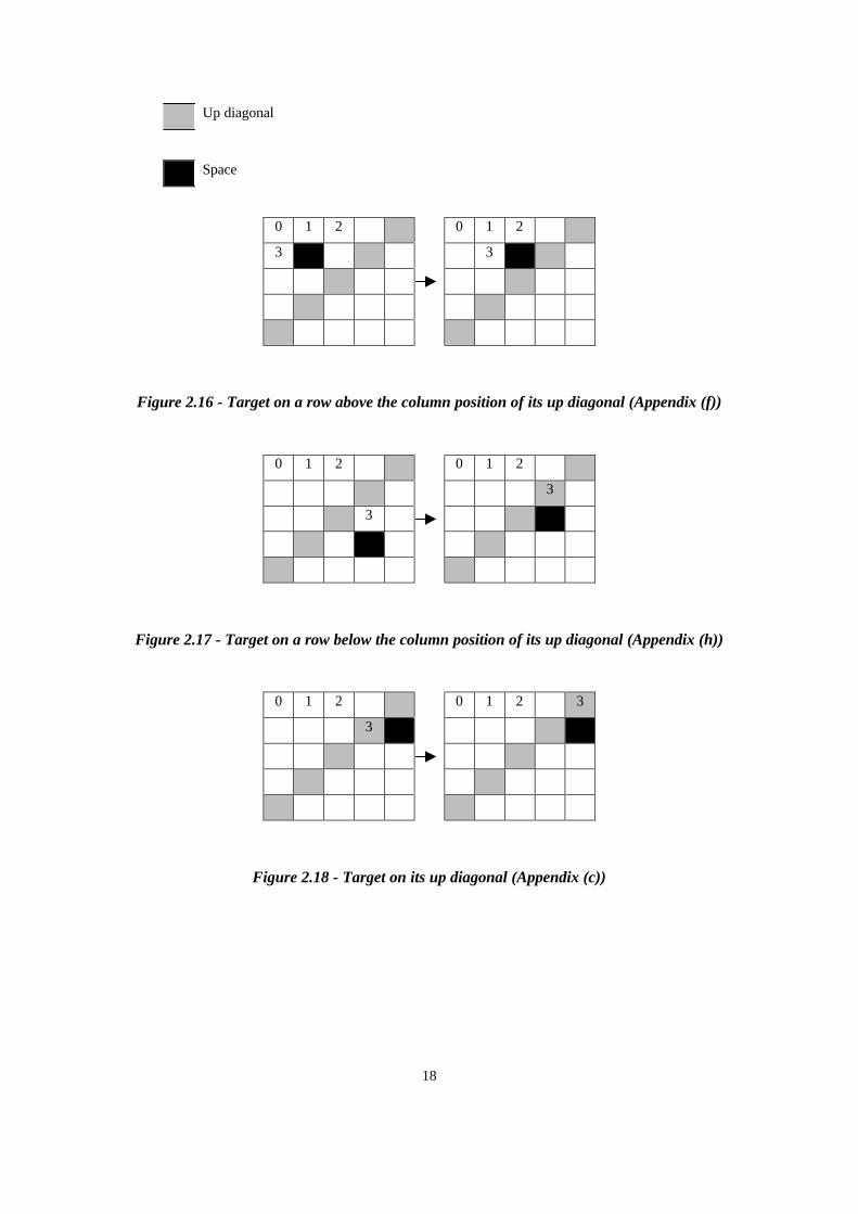
As before, the target is either on a row below, on or above the column position of the

target’s up diagonal. If the target is above, then the target is horizontally moved right

onto its up diagonal (Figure 2.16). If the target is below, then the target is vertically

moved up onto its up diagonal (Figure 2.17). When the target is on its up diagonal, it

is diagonally moved right up one row until the target is in the rowend location

(Figure 2.18).

18

Up diagonal

Space

0 1 2 0 1 2

3 3

Figure 2.16 - Target on a row above the column position of its up diagonal (Appendix (f))

0 1 2 0 1 2

3

3

Figure 2.17 - Target on a row below the column position of its up diagonal (Appendix (h))

0 1 2 0 1 2 3

3

Figure 2.18 - Target on its up diagonal (Appendix (c))

19

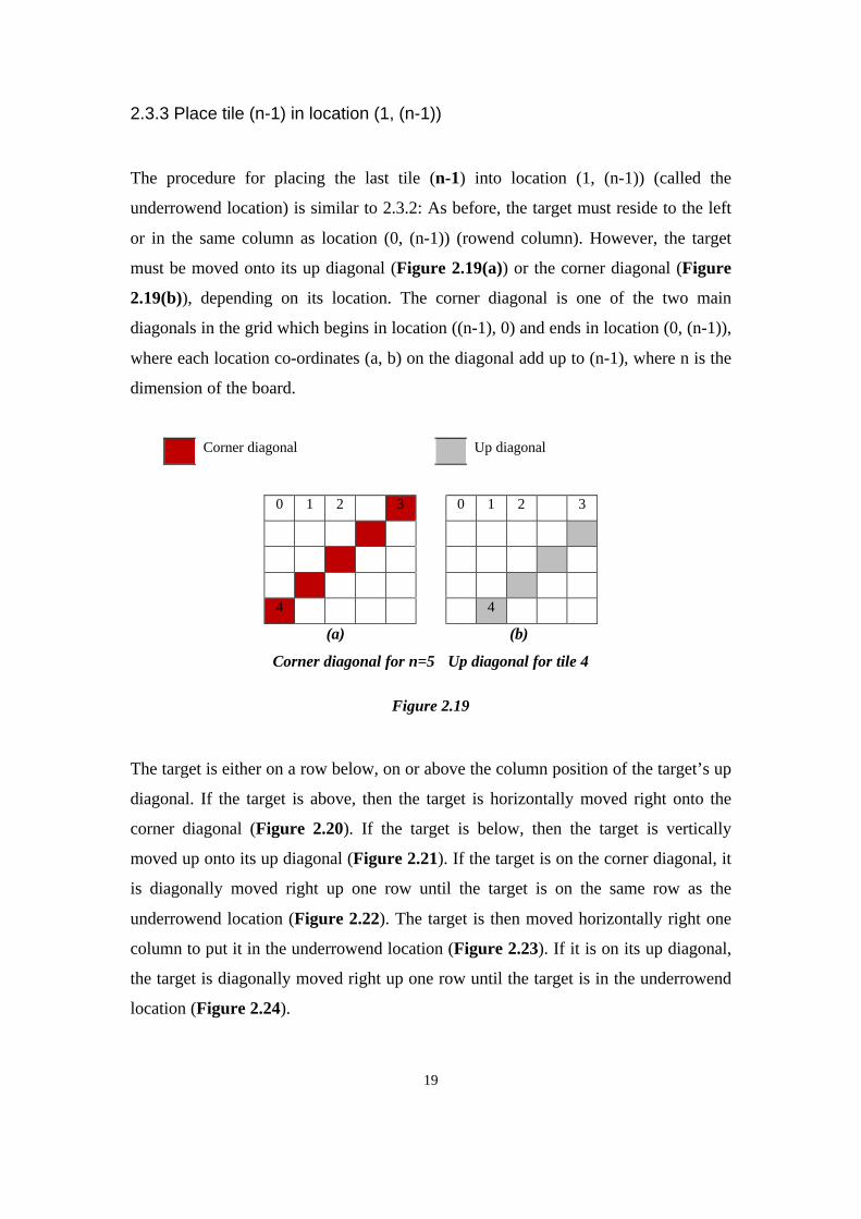
2.3.3 Place tile (n-1) in location (1, (n-1))

The procedure for placing the last tile (n-1) into location (1, (n-1)) (called the

underrowend location) is similar to 2.3.2: As before, the target must reside to the left

or in the same column as location (0, (n-1)) (rowend column). However, the target

must be moved onto its up diagonal (Figure 2.19(a)) or the corner diagonal (Figure

2.19(b)), depending on its location. The corner diagonal is one of the two main

diagonals in the grid which begins in location ((n-1), 0) and ends in location (0, (n-1)),

where each location co-ordinates (a, b) on the diagonal add up to (n-1), where n is the

dimension of the board.

Corner diagonal Up diagonal

0 1 2 3 0 1 2 3

4 4

(a) (b)

Corner diagonal for n=5 Up diagonal for tile 4

Figure 2.19

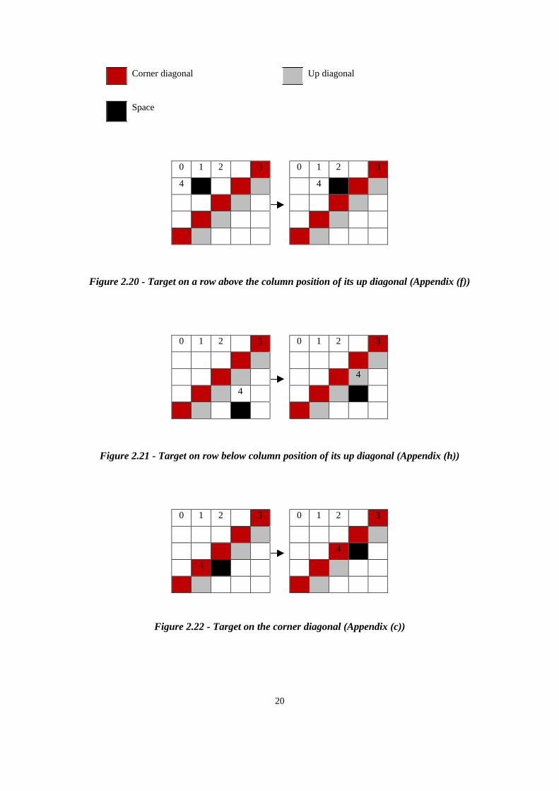
The target is either on a row below, on or above the column position of the target’s up

diagonal. If the target is above, then the target is horizontally moved right onto the

corner diagonal (Figure 2.20). If the target is below, then the target is vertically

moved up onto its up diagonal (Figure 2.21). If the target is on the corner diagonal, it

is diagonally moved right up one row until the target is on the same row as the

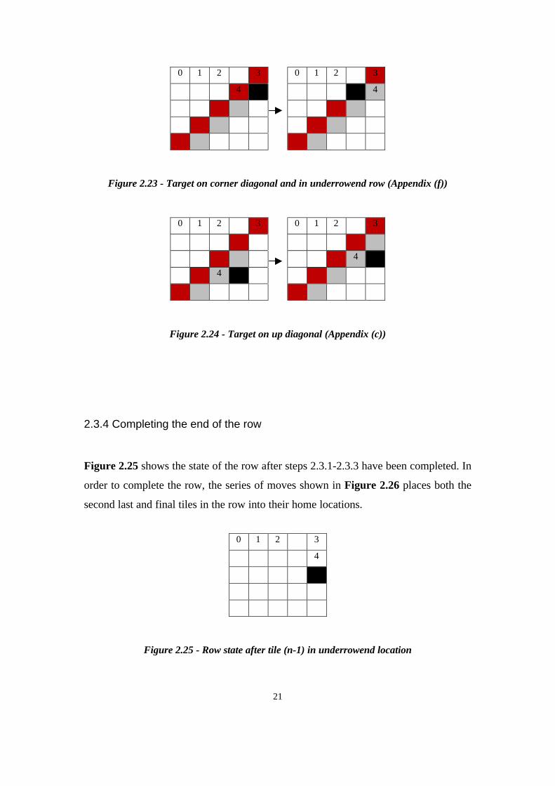
underrowend location (Figure 2.22). The target is then moved horizontally right one

column to put it in the underrowend location (Figure 2.23). If it is on its up diagonal,

the target is diagonally moved right up one row until the target is in the underrowend

location (Figure 2.24).

20

Corner diagonal Up diagonal

Space

0 1 2 3 0 1 2 3

4 4

Figure 2.20 - Target on a row above the column position of its up diagonal (Appendix (f))

0 1 2 3 0 1 2 3

4

4

Figure 2.21 - Target on row below column position of its up diagonal (Appendix (h))

0 1 2 3 0 1 2 3

4

4

Figure 2.22 - Target on the corner diagonal (Appendix (c))

21

0 1 2 3 0 1 2 3

4 4

Figure 2.23 - Target on corner diagonal and in underrowend row (Appendix (f))

0 1 2 3 0 1 2 3

4

4

Figure 2.24 - Target on up diagonal (Appendix (c))

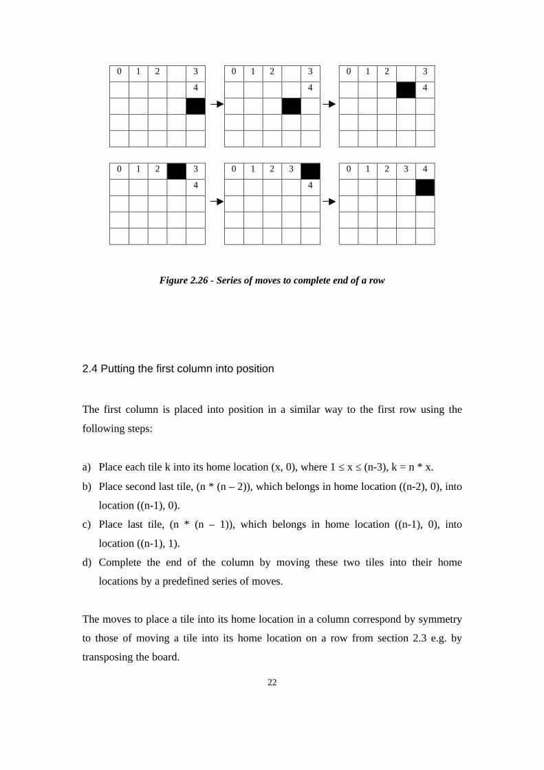
2.3.4 Completing the end of the row

Figure 2.25 shows the state of the row after steps 2.3.1-2.3.3 have been completed. In

order to complete the row, the series of moves shown in Figure 2.26 places both the

second last and final tiles in the row into their home locations.

0 1 2 3

4

Figure 2.25 - Row state after tile (n-1) in underrowend location

22

0 1 2 3 0 1 2 3 0 1 2 3

4 4 4

0 1 2 3 0 1 2 3 0 1 2 3 4

4 4

Figure 2.26 - Series of moves to complete end of a row

2.4 Putting the first column into position

The first column is placed into position in a similar way to the first row using the

following steps:

a) Place each tile k into its home location (x, 0), where 1 ≤ x ≤ (n-3), k = n * x.

b) Place second last tile, (n * (n – 2)), which belongs in home location ((n-2), 0), into

location ((n-1), 0).

c) Place last tile, (n * (n – 1)), which belongs in home location ((n-1), 0), into

location ((n-1), 1).

d) Complete the end of the column by moving these two tiles into their home

locations by a predefined series of moves.

The moves to place a tile into its home location in a column correspond by symmetry

to those of moving a tile into its home location on a row from section 2.3 e.g. by

transposing the board.

23

3 Special Board Configurations

There are certain board configurations that cannot be solved using the methods

employed in the algorithm above. As a result, these configurations have to be handled

in such a way so that the board is placed into a position so that the above algorithm

can be used to solve it.

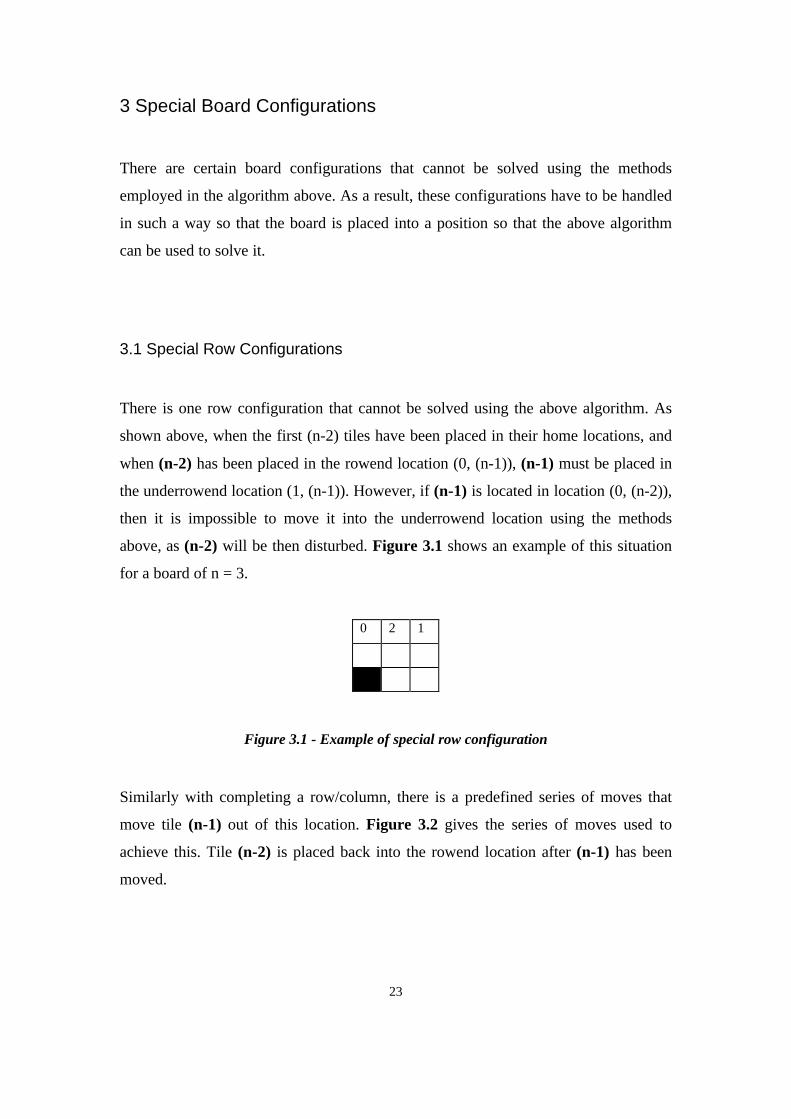
3.1 Special Row Configurations

There is one row configuration that cannot be solved using the above algorithm. As

shown above, when the first (n-2) tiles have been placed in their home locations, and

when (n-2) has been placed in the rowend location (0, (n-1)), (n-1) must be placed in

the underrowend location (1, (n-1)). However, if (n-1) is located in location (0, (n-2)),

then it is impossible to move it into the underrowend location using the methods

above, as (n-2) will be then disturbed. Figure 3.1 shows an example of this situation

for a board of n = 3.

0 2 1

Figure 3.1 - Example of special row configuration

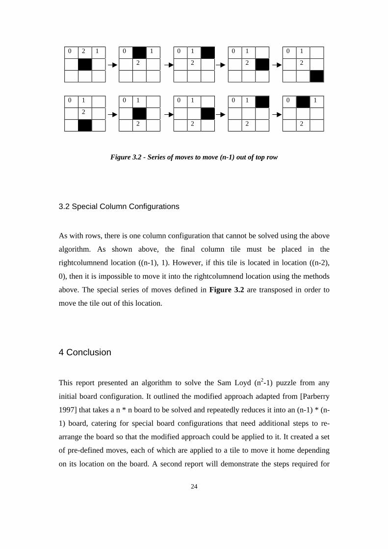
Similarly with completing a row/column, there is a predefined series of moves that

move tile (n-1) out of this location. Figure 3.2 gives the series of moves used to

achieve this. Tile (n-2) is placed back into the rowend location after (n-1) has been

moved.

24

0 2 1 0 1 0 1 0 1 0 1

2 2 2 2

0 1 0 1 0 1 0 1 0 1

2

2 2 2 2

Figure 3.2 - Series of moves to move (n-1) out of top row

3.2 Special Column Configurations

As with rows, there is one column configuration that cannot be solved using the above

algorithm. As shown above, the final column tile must be placed in the

rightcolumnend location ((n-1), 1). However, if this tile is located in location ((n-2),

0), then it is impossible to move it into the rightcolumnend location using the methods

above. The special series of moves defined in Figure 3.2 are transposed in order to

move the tile out of this location.

4 Conclusion

This report presented an algorithm to solve the Sam Loyd (n2-1) puzzle from any

initial board configuration. It outlined the modified approach adapted from [Parberry

1997] that takes a n * n board to be solved and repeatedly reduces it into an (n-1) * (n-

1) board, catering for special board configurations that need additional steps to re-

arrange the board so that the modified approach could be applied to it. It created a set

of pre-defined moves, each of which are applied to a tile to move it home depending

on its location on the board. A second report will demonstrate the steps required for

25

determining the upper bound of moves for a board of a given dimension and show

that the modified algorithm solves a worst case board in less moves than Parberry's.

The algorithm to solve the Loyd Puzzle was developed in order to test the suitability

of updateable arrays in functional programming languages as a tool to develop

efficient, correct programs. Two types of updateable array were chosen - Concurrent

Clean's unique array and Haskell's monadic array. The functional implementation of

the Loyd algorithm was designed in such a way that data required to generate a board

solution would be used cost-effectively. The results of these tests on the Sam Loyd

puzzle and other problems can be found in a future report.

26

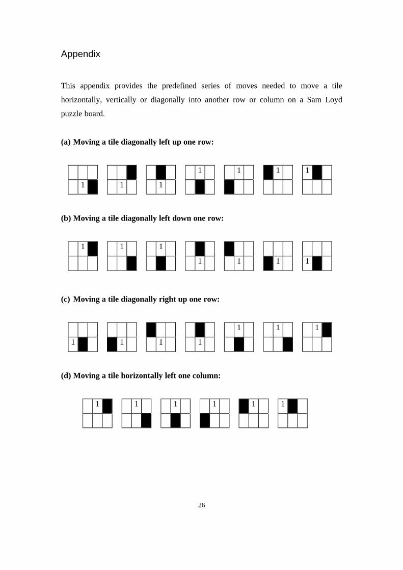
Appendix

This appendix provides the predefined series of moves needed to move a tile

horizontally, vertically or diagonally into another row or column on a Sam Loyd

puzzle board.

(a) Moving a tile diagonally left up one row:

1 1 1 1

1 1 1

(b) Moving a tile diagonally left down one row:

1 1 1

1 1 1 1

(c) Moving a tile diagonally right up one row:

1 1 1

1 1 1 1

(d) Moving a tile horizontally left one column:

1 1 1 1 1 1

27

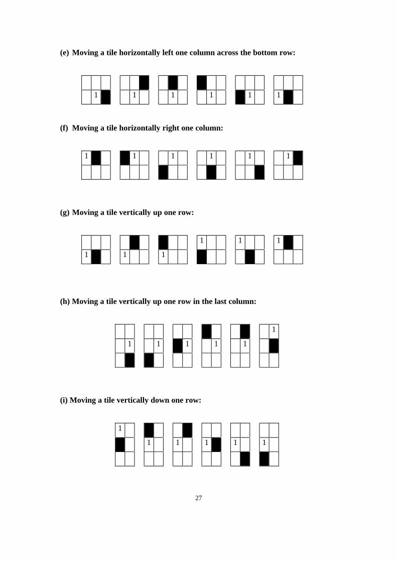
(e) Moving a tile horizontally left one column across the bottom row:

1 1 1 1 1 1

(f) Moving a tile horizontally right one column:

1 1 1 1 1 1

(g) Moving a tile vertically up one row:

1 1 1

1 1 1

(h) Moving a tile vertically up one row in the last column:

1

1 1 1 1 1

(i) Moving a tile vertically down one row:

1

1 1 1 1 1

28

References

Bird, R. and Wadler, P. Introduction to Functional Programming. Prentice Hall, 1988.

Gardner, M. Mathematical Puzzles and Diversions. Bell, 1961.

Parberry, I. A Real Time Algorithm for the (n2 – 1) Puzzle. Information Processing

Letters, Vol. 56, pp. 23-28, 1997.

Schofield, P. D. A. Complete solution of the Eight Puzzle. In Machine Intelligence by

N. L. Collins and D. Michie, pages 125-133. American Elsevier, 1967.

Storey, W.E. Notes on the 15 puzzle 2. American Journal of Mathematics, 2(4):399-

404, 1879.