Embed Size (px)
Citation preview

The relationship between dry rock bulk modulus and porosity – an empirical study
Brian Russell* and Tad Smith
Hampson-Russell, A CGGVeritas Company* Adjunct Professor, University of Calgary

Introduction
There are various approaches to computing Kdry as a function of porosity, and thus inferring changes in fluid content as a function of porosity.One common approach is the pore space stiffness method, and a second approach uses critical porosity.Mavko and Mukerji (1995) propose a useful template for plotting the various porosity functions. Using a dataset collected by De Hua Han, and the Mavko-Mukerji template, we will evaluate the suitability of each method.Using the Han dataset, we will also derive an empirical relationship between pore space stiffness and pressure.
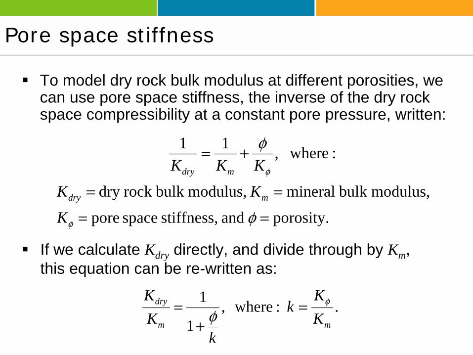
Pore space stiffness
To model dry rock bulk modulus at different porosities, we can use pore space stiffness, the inverse of the dry rock space compressibility at a constant pore pressure, written:
porosity. and stiffness, space poremodulus,bulk mineral modulus,bulk rock dry
: where,11
==
==
+=
φ
φ
φ
φ
KKKKKK
mdry
mdry
If we calculate Kdry directly, and divide through by Km, this equation can be re-written as:
. :where,1
1
mm
dry
KK
k
kKK φ
φ =+
=

Constant pore space stiffness
k = 0.5
k = 0.05k = 0.01k = 0.1
k = 0.3
Note that a family of constant kcurves can be drawn on a plot of Kdry /Km versus porosity, allowing us to estimate Kφtrends from rock physics measurements.

Voigt and Reuss bounds
Mavko and Mukerji,(1995), discuss other models such as the Voigt (high bound) and Reuss (low bound) averages, given by:
( ) ( ) φφφφ −=⇒−≈+−= 111m
Voigtdry
mairmVoigtdry K
KKKKK
011
≈⎥⎦
⎤⎢⎣
⎡+−=
−
airm
Ruessdry KK
K φφ
The critical porosity model (Nur, 1992) is given by:
porosity. critical where,111 =−≈⎟⎟⎠
⎞⎜⎜⎝
⎛−−= c
cm
Voigtdry
cm
dry
KK
KK
φφφ
φφ
φc separates load-bearing sediments (φ < φc) from suspensions (φ > φc) and is like a scaled Voigt model.
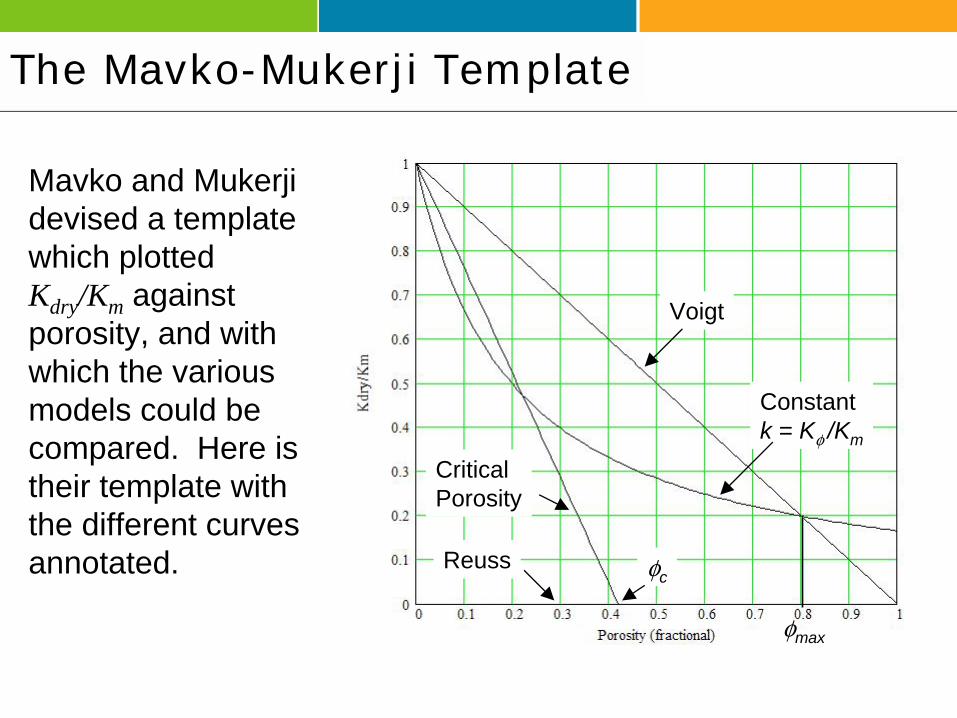
The Mavko-Mukerji Template
Mavko and Mukerjidevised a template which plotted Kdry/Km against porosity, and with which the various models could be compared. Here is their template with the different curves annotated.
Voigt
Constant k = Kφ /Km
Critical Porosity
Reuss φc
φmax

Han’s Dataset
To test the various models, Mavko and Mukerji (1995) used a dataset collected by De Hua Han for his 1986 Ph.D. thesis. This dataset was graciously provided to us by Dr. Han of the University of Houston.Han’s dataset consisted of a number of sandstones of various porosities and clay content, measured at different pressures and saturations.Han was able to derive empirical formulae for P and S-wave velocities versus porosity and clay content (Han et al., 1986).From Han’s measurements, Mavko and Mukerji (1995) used the 10 clean sandstones at 40 MPa and a single clean sandstone at 5, 10, 20, 30, and 40 MPa.

Data points used by Mavko and Mukerji
Figure (a) shows the ten clean dry sandstones at a constant pressure of 40 MPa. Figure (b) shows a single clean dry sandstone at pressures of 5, 10, 20, 30, and 40 Mpa. The dotted line is the Voigt limit.
(a) (b)
Decreasing Pressure
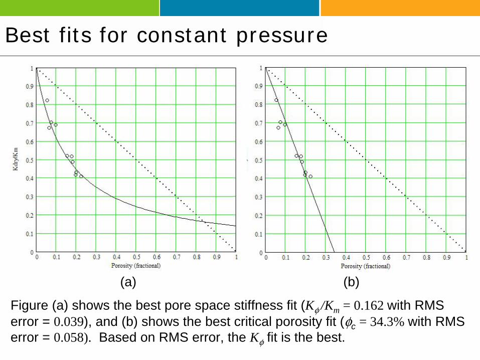
Best fits for constant pressure
Figure (a) shows the best pore space stiffness fit (Kφ /Km = 0.162 with RMS error = 0.039), and (b) shows the best critical porosity fit (φc = 34.3% with RMS error = 0.058). Based on RMS error, the Kφ fit is the best.
(a) (b)

Modeling Kdry versus porosity
To model Kdry at different porosities using pore space stiffness, Kφ can be calculated for the in-situ porosity using the original equation:
11111
−
−−
⎥⎥⎦
⎤
⎢⎢⎣
⎡−=⇒−=
mdrysituin
mdry
situin
KKK
KKKφφ
φφ
Once we have estimated the in-situ value for the pore space stiffness, we can calculate a value for Kdry at a new porosity at the same pressure using:
1
_1
−
⎥⎥⎦
⎤
⎢⎢⎣
⎡+=
m
newnewdry KK
Kφ
φ

Modeling μ versus porosity
situindry
newdrysituinnew K
K
−−=
_
_μμ
Murphy et al (1993) measured Kdry and μ for clean quartz sandstones, and found the ratio of Kdry/μ is constant for varying porosity. We can therefore compute the new value of μ from:
The figure on the next slide shows a cross-plot of VP/VSratio versus P-impedance as a function of porosity and water saturation in a gas-charged sand using the following three assumptions:
Biot-Gassmann is used to model fluid changesThe pore space stiffness is used to model Kdry vs porosity change.The above equation is used to model μ vs porosity change.

VP/VS Ratio vs P-Impedance
wet
gas
φ = 5%
15%
φ = 50%
33%

Variable pressure
Next, consider the variable pressure case. Figure (a) shows that k = Kφ /Km decreases as pressure decreases. Figure (b) shows that φc also decreases with decreasing pressure.
(a) (b)
φc decreases
k = Kφ /Kmdecreases
Decreasing Pressure
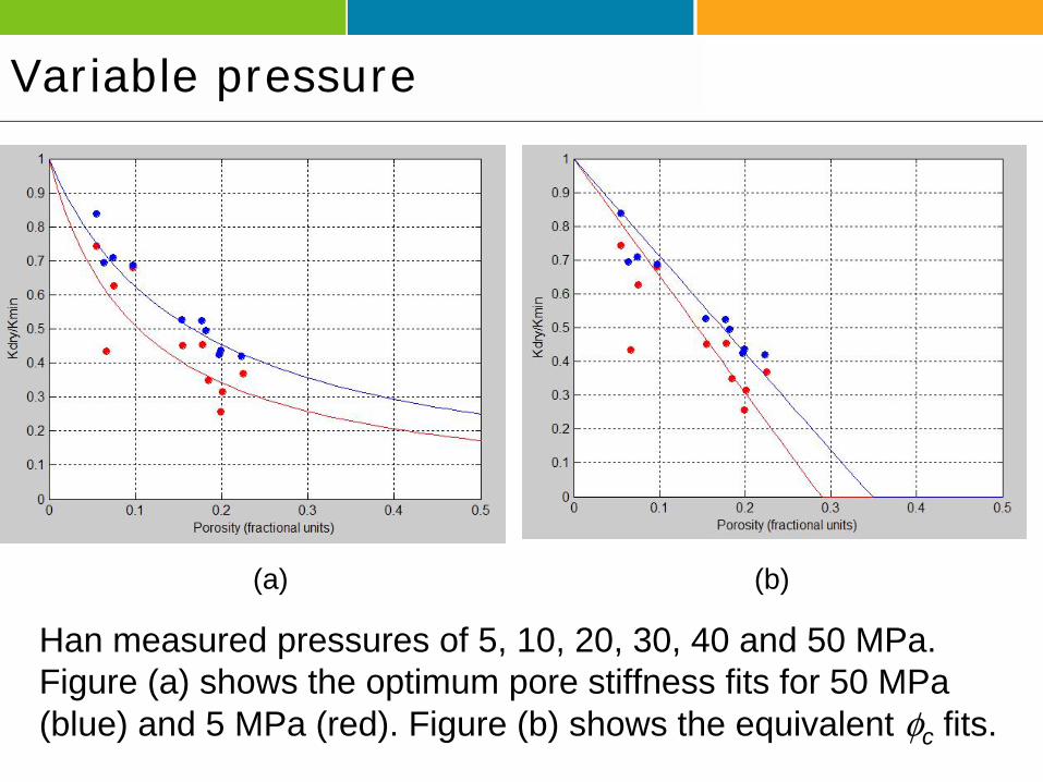
Variable pressure
Han measured pressures of 5, 10, 20, 30, 40 and 50 MPa. Figure (a) shows the optimum pore stiffness fits for 50 MPa(blue) and 5 MPa (red). Figure (b) shows the equivalent φc fits.
(a) (b)
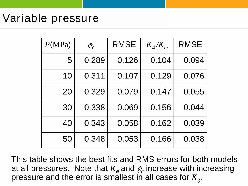
Variable pressure
This table shows the best fits and RMS errors for both models at all pressures. Note that Kφ and φc increase with increasing pressure and the error is smallest in all cases for Kφ.
0.0380.1660.0530.34850
0.0390.1620.0580.34340
0.0440.1560.0690.33830
0.0550.1470.0790.32920
0.0760.1290.1070.31110
0.0940.1040.1260.2895
RMSEKφ /KmRMSEφcP(MPa)
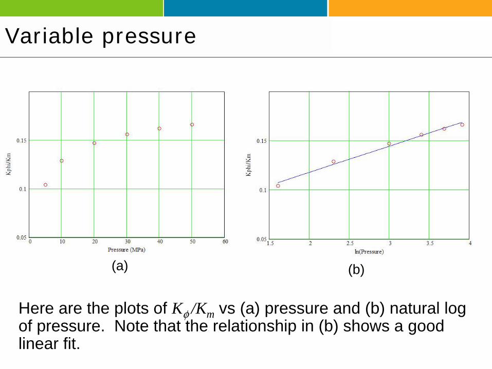
Variable pressure
Here are the plots of Kφ /Km vs (a) pressure and (b) natural log of pressure. Note that the relationship in (b) shows a good linear fit.
(a) (b)

Variable pressure
From this equation, we can derive the relationship between change in pore space stiffness and pressure:
PPKK
PK
PK
dPdK
mm Δ=Δ⇒=
ΔΔ
≈ 027.0027.0φ
φφ
This equation allows us derive constant Kφ curves at different pressures than the in-situ pressure, and hence predict a depth variable Kdry versus porosity relationship.
)ln(027.0065.0 PKK
m
+=φ
From the previous plot, the best least-squares fit is:

Carbonate example
Finally, Baechle et al. (2006) modeled carbonates using pore space stiffness. They show that dolomites with microporosity(blue points on right) fit the curve k = 0.2and dolomites with vuggy porosity (red) fit the curve k = 0.1. The dashed line is the critical porosity fit.
Baechle et al. (2006)
microporosityvuggy porosity
k = 0.1k = 0.2

ConclusionsWe have reviewed the two different approaches (pore space stiffness and critical porosity) to model porosity changes in fluid-saturated rocks using the dry rock bulk modulus.When tested using Han’s measurements, the pore space stiffness method gave the best fit to the data.We then showed a model incorporating the pore space stiffness method with Biot-Gassmann fluid changes.We next derived an equation that allowed us to calculate pore space stiffness as a function of pressure.Finally, we looked at a carbonate example from the literature using the critical porosity method. Limitations of this study were that only clean sandstones were modeled and that the pore space stiffness method is appropriate only at porosities much less than critical porosity.

References
Baechle, G.T., Weger, R., Eberli, G.P., and Colpaert, A., 2006, Pore size and pore type effects on velocity – Implications for carbonate rock physics models: Abstract of paper presented at “Sound of Geology” workshop in Bergen, Norway.
Han, D., 1986, Effects of porosity and clay content on acoustic properties of sandstones and unconsolidated sediments: Ph.D. dissertation, Stanford University.
Han, D.H., A. Nur, and D. Morgan, 1986, Effects of porosity and clay content on wave velocities in sandstones: Geophysics, 51, 2093-2107.
Mavko, G., and T. Mukerji, 1995, Seismic pore space compressibility and Gassmann\'s relation: Geophysics, 60, 1743-1749.
Murphy, W., Reischer, A., and Hsu, K., 1993, Modulus Decomposition of Compressional and Shear Velocities in Sand Bodies: Geophysics, 58, 227-239.
Nur, A., 1992, Critical porosity and the seismic velocities in rocks: EOS, Transactions American Geophysical Union, 73, 43-66.


![Pressure Derivatives of Bulk Modulus, Thermal Expansivity ... · has large bulk modulus, less compressibility and high melting temperature [9, 10]. MgO remains stable in the rock](https://img.pdfslide.us/doc/110x75/6062334e70cf1b4132608fe7/pressure-derivatives-of-bulk-modulus-thermal-expansivity-has-large-bulk-modulus.jpg)