Embed Size (px)
Citation preview
CENTRE FOR DYNAMIC MACROECONOMIC ANALYSIS CONFERENCE PAPERS 2006
CASTLECLIFFE, SCHOOL OF ECONOMICS & FINANCE, UNIVERSITY OF ST ANDREWS, KY16 9AL
TEL: +44 (0)1334 462445 FAX: +44 (0)1334 462444 EMAIL: [email protected] www.st-andrews.ac.uk/cdma
CDMC06/10
The New Consensus in Monetary Policy: Is the NKM fit for the purpose of inflation
targeting?
Peter N. Smith*
University of York Mike Wickens†
University of York and CEPR
SEPTEMBER 2006
ABSTRACT
In this paper we examine whether or not the NKM is .t for the purpose of providing a suitable basis for the conduct of monetary policy through inflation targeting. We focus on a number of issues: the dynamic response of inflation to interest rates in a theoretical NKM under discretion and commitment to a Taylor rule; the implications for the specification of the New Keynesian Phillips equation of alternative models of imperfect competition in a closed and an open economy; the general equilibrium underpinnings of the IS function; the extent of empirical support for the NKM; what the empirical evidence on the NKM implies for inflation targeting. Our findings reveal a number of problems with the NKM. Theoretically, the NKM predicts that a discretionary increase in interest rates will increase inflation, not reduce it. This is supported by our VAR evidence. Estimates of the NKM indicate a negative relation between interest rates and inflation, but the signs in the structural equations are inconsistent with the theory. We conclude that the standard specifications of the inflation and output equations are inadequate and that these equations should be embedded in a larger model.
Keywords: Inflation targeting, monetary policy, New Keynesian model JEL Classification: E3, E5
* Department of Economics, University of York, York, YO10 5DD, UK, email: [email protected] . † Department of Economics, University of York, York, YO10 5DD, UK, email: [email protected].

1 Introduction
The new consensus in monetary policy is based on in�ation targeting carried out by a central bank
setting a short-term interest rate using its discretion rather than following a formal rule. The
theoretical basis of in�ation targeting is a simple two-equation model of the in�ationary process
consisting of an expectations augmented Phillips equation for in�ation and an output equation
derived loosely from an inter-temporal model of the economy called the new �IS�function. This
model is commonly known as the New Keynesian model (NKM).1 This re�ects the introduction
of price stickiness through a Phillips equation in a dynamic stochastic general equilibrium (DSGE)
model of the economy. Even when a larger model of the economy is employed in in�ation targeting,
such as the Bank of England�s new quarterly model, see Bank of England (2005), these two
equations usually form its core.
In this paper we examine whether or not the NKM is �t for the purpose of providing a suitable
basis for the conduct of monetary policy through in�ation targeting. We focus on a number of
issues: the dynamic response of in�ation to interest rates in a theoretical NKM under discretion
and commitment to a Taylor rule; the implications for the speci�cation of the New Keynesian
Phillips equation of alternative models of imperfect competition in a closed and an open economy;
the general equilibrium underpinnings of the IS function; the extent of empirical support for the
NKM; what the empirical evidence on the NKM implies for in�ation targeting and whether this
is consistent with evidence from an atheoretical VAR.
Although there seems to be little disagreement about basing in�ation targeting on the NKM,
it can be shown that the relation between in�ation and interest rates depends on whether a policy
of discretion or commitment is used. Under a policy of discretion an increase in interest rates will
raise in�ation not reduce it; however, under a policy of commitment to a Taylor rule a positive
interest rate shock is predicted to reduce in�ation.
1 There is a vast literature on in�ation targeting via the NKM. For recent surveys see Clarida, Gali and Gertler(1999), Walsh (2003), Woodford (2003) and Bernanke and Woodford (2005).
2

There is much less agreement on how to specify the two equations of the NKM. This has
considerable signi�cance for the transmission mechanism, and hence the potential e¤ectiveness, of
monetary policy. For example, the precise role of output in these new formulations of the Phillips
equation is largely unresolved. This is a crucial question as monetary policy in the NKM works
through interest rates a¤ecting output, and output a¤ecting in�ation. For monetary policy to be
e¤ective both links must be strong. In early versions of the New Keynesian Phillips equation,
in�ation was related to the output gap. More recently, attempts have been made to base the
Phillips equation on �rmer micro foundations in which �rms have a degree of monopolistic control
over prices with the consequence that cost increases and changes in the price mark-up due to
demand �uctuations directly determine prices. They are passed on over time as prices display
stickiness. The result has been a partial return to the old-style Phillips equation with costs being
the main determinant of prices along with demand, but with the addition of forward-lookingness
in price setting.
Most of the research on in�ation targeting and the NKM has assumed a closed economy. In
an open economy, however, the exchange rate may also play an important role in the transmission
mechanism. Changes in the exchange rate, perhaps as a result of domestic monetary policy, may
a¤ect costs more directly and the impact on prices would not be dependent on the output part
of the transmission mechanism. Considerations of imperfect competition in�uence the strength of
this e¤ect. In a large open economy, importers are more likely to price to the domestic market
than in a small open economy which is more likely to have to accept world prices denominated in
foreign currency. Hence, the exchange rate channel becomes more important in a small than in
a large open economy. Perhaps this explains why the Bank of England places the exchange rate
fourth in its list of channels for the transmission mechanism.2
The speci�cation of the New Keynesian output equation has proved less contentious than
that of the in�ation equation. It is based on the consumption Euler equation of a DSGE model.
2 See Bank of England (1999).
3

This equation is commonly interpreted as implying that an increase in the current interest rate
will reduce consumption, and hence output. We argue in this paper that this is an incorrect
interpretation. It assumes that expected future consumption (output) is given, which logically it
is not as it is determined simultaneously with current consumption. Strictly, the Euler equation
determines the response of the expected future change in consumption to an expected future change
in the interest rate. To �nd the e¤ect on current consumption of a change in the current interest
rate it is necessary to derive the consumption function by combining the Euler equation with the
inter-temporal budget constraint. It then becomes clear that the sign of this e¤ect depends on
whether households hold net assets or net liabilities. Following an increase in the current interest
rate, consumption will only decrease if households hold net liabilities. In our view this seriously
undermines the usefulness of the NKM.
The aim of monetary policy is to return in�ation to its target level following (or in anticipation
of) shocks to the economy. The NKM, with its emphasis on using interest rates to control output,
is much better suited to dealing with demand than supply shocks as it raises no con�ict between
the objectives of in�ation and output stabilization. A positive demand shock raises output, and
hence in�ation, and this is o¤set by raising interest rates. But a supply shock will raise in�ation
and reduce output. An increase in interest rates to control in�ation will further reduce output.
In�ation and output control are now in con�ict. Little is known about the size of the output costs
of in�ation control following a supply shock.
The paper is set out as follows. In Section 2 we analyse the dynamic response of in�ation
to interest rates under discretion and commitment to a Taylor rule. In Section 3 we discuss the
speci�cation of the New Keynesian Phillips equation under imperfect competition in a closed and
an open economy. We consider the general equilibrium underpinnings of the IS function in Section
4. In Section 5 we provide estimates of various speci�cations of the NKM based on UK quarterly
data 1970-2005. In Section 6 we analyse the implications of these estimates for in�ation targeting
and compare these with the impulse responses from a VAR based on the NKM. We present our
4
conclusions in Section 7.
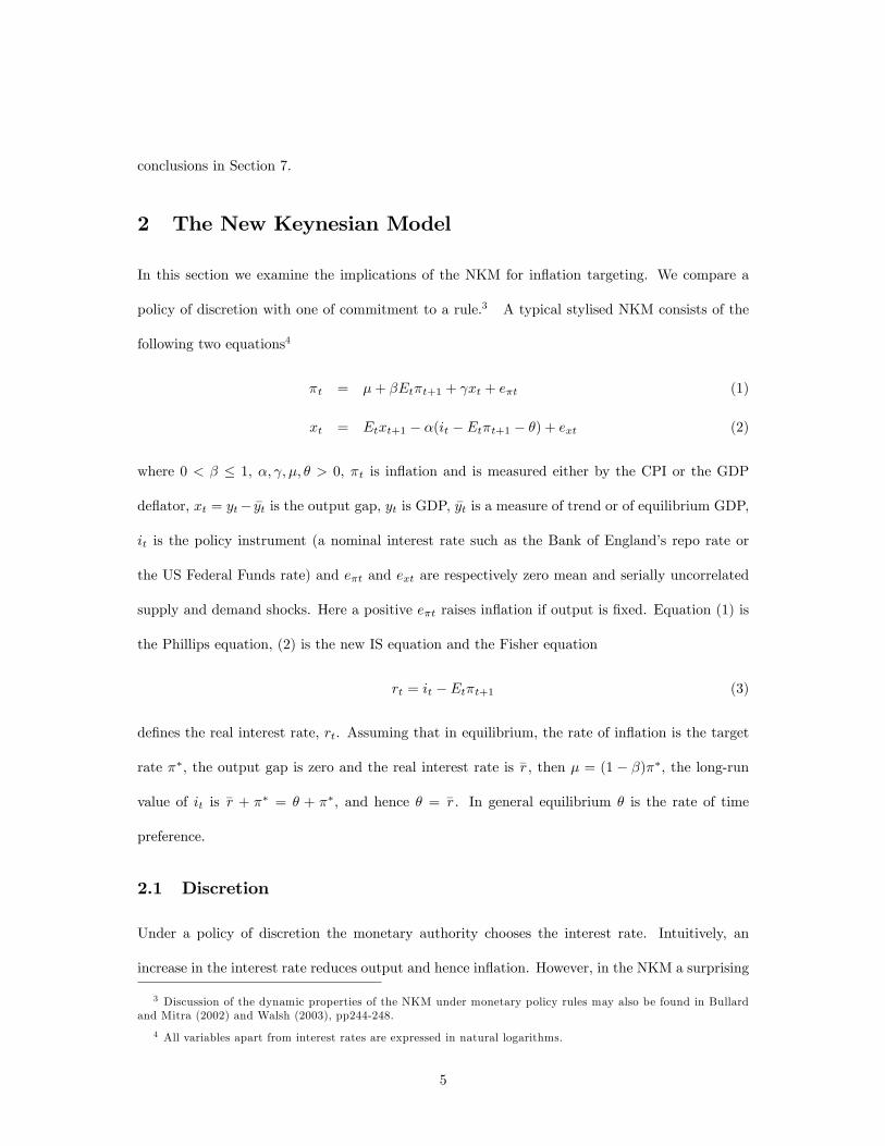
2 The New Keynesian Model
In this section we examine the implications of the NKM for in�ation targeting. We compare a
policy of discretion with one of commitment to a rule.3 A typical stylised NKM consists of the
following two equations4
�t = �+ �Et�t+1 + xt + e�t (1)
xt = Etxt+1 � �(it � Et�t+1 � �) + ext (2)
where 0 < � � 1, �; ; �; � > 0, �t is in�ation and is measured either by the CPI or the GDP
de�ator, xt = yt�_yt is the output gap, yt is GDP,
_yt is a measure of trend or of equilibrium GDP,
it is the policy instrument (a nominal interest rate such as the Bank of England�s repo rate or
the US Federal Funds rate) and e�t and ext are respectively zero mean and serially uncorrelated
supply and demand shocks. Here a positive e�t raises in�ation if output is �xed. Equation (1) is
the Phillips equation, (2) is the new IS equation and the Fisher equation
rt = it � Et�t+1 (3)
de�nes the real interest rate, rt. Assuming that in equilibrium, the rate of in�ation is the target
rate ��, the output gap is zero and the real interest rate is_r , then � = (1 � �)��, the long-run
value of it is_r + �� = � + ��, and hence � =
_r . In general equilibrium � is the rate of time
preference.
2.1 Discretion
Under a policy of discretion the monetary authority chooses the interest rate. Intuitively, an
increase in the interest rate reduces output and hence in�ation. However, in the NKM a surprising
3 Discussion of the dynamic properties of the NKM under monetary policy rules may also be found in Bullardand Mitra (2002) and Walsh (2003), pp244-248.
4 All variables apart from interest rates are expressed in natural logarithms.
5

result occurs. Eliminating yt from the model gives the following dynamic equation for �t
�t � (1 + � + � )Et�t+1 + �Et�t+2 = �� � � it + e�t + ext
The long-run solution is
�t = it � �
To analyse the short-run dynamics we note that the auxiliary equation is
�(L) = 1� (1 + � + � )L�1 + �L�2 = 0
where Et�t+n = L�n�t. Setting L = 1 gives �(1) = �� < 0. Therefore, despite having forward
expectations and no lags, the solution of the equation is a saddlepath with one of the roots greater
than unity and the other less than unity; both are positive. Denoting the roots by �1 > 1 and
�2 < 1 it can be shown (see Wickens (1993) for details) that the solution can be written as
�t = ���
�1+ �1�t�1 +
�
�1(�1s=0�
�(s+1)2 Etit+s + it�1) + ��e�t + �xext �
1
�1(e�;t�1 + ex;t�1)
where �� and �x are arbitrary constants, implying that the solution is not unique. It follows that
a discretionary increase in interest rates either in the previous period, the current period or in
the future is expected to increase, not decrease, in�ation as the above intuition might lead one
to expect. Moreover, the appropriate setting for interest rates to counteract current supply and
demand shocks is unclear as their e¤ect on in�ation is indeterminate. It would seem therefore that
the use of the NKM under discretion does not provide a satisfactory basis for in�ation targeting.
2.2 Rules based monetary policy
It is informative to compare the solution under a policy of discretion with that in which interest
rates are determined under commitment to a Taylor rule. The standard Taylor rule is
it = � + �� + �(�t � ��) + �xt + eit
6

with � = 1:5 and � = 0:5. The random variable eit is introduced to allow for unexpected departures
from the rule. Solving the NKM together with the Taylor rule results in both xt and it being
eliminated and gives
[1 + �(� + � )]�t � [1 + �(1 + ��) + � ]Et�t+1 + �Et�t+2 = zt
zt = ���[�(1� �) + (�� 1)] + (1 + ��)e�t � Ete�;t+1 + ext � � eit
The auxiliary equation is
�(L) = [1 + �(� + � )]� [1 + �(1 + ��) + � ]L�1 + �L�2 = 0
As �(1) = �[�(1� �) + (�� 1)] > 0 and 1 > �1+�(�+� ) > 0 the roots of the auxiliary equation
lie inside the unit circle and hence the model is globally unstable. It can be shown (see Wickens
(1993)) that there is now a unique solution and this can be written as
�t =1
1 + �(� + � )[
�1�1 � �2
�1s=0�s1Etzt+s �
�2�1 � �2
�1s=0�s2Etzt+s]
= �� +1
1 + �(� + � )[(1 + ��)e�t + ext � � eit]
Thus in�ation deviates from target due to the three shocks. Positive in�ation and output shocks
cause in�ation to rise above target, but positive interest rate shocks cause in�ation to fall below
target. We note that a forward-looking Taylor rule in which Et�t+1 replaces �t and Etxt+1
replaces xt gives a similar result.
If the NKM is a good representation of the economy then these results support a policy
of commitment to a rule. We now investigate whether the NKM is a suitable representation
by examining the speci�cation of each equation in more detail. First we consider the Phillips
equation.
7
3 The New Keynesian Phillips equation
3.1 Which in�ation measure to use?
The �rst issue to address is the measure of in�ation to target. We can then discuss how this
measure should be determined. Arguably, only two measures are worth considering. These are
CPI in�ation and the GDP de�ator. Broadly, the GDP de�ator measures the price of domestic
production, whereas the CPI measures the price of domestic consumption which has greater re-
sponse to import prices. The more open the economy, the larger are likely to be the di¤erences
between the two.
A distinction is often made between �core� and �headline� in�ation. The GDP de�ator is
closely related to core in�ation whereas the CPI, which is a¤ected by external in�uences, corre-
sponds more to headline in�ation. The Treasury�s original remit to the Bank of England was to
target �prices in the shops�. A measure of the CPI was chosen which excludes mortgage interest
payments in order to avoid in�ation being directly a¤ected by changes in interest rates. Although
central banks typically target CPI in�ation, most econometric work uses the GDP de�ator.
3.2 Some general theoretical considerations
In�ation equations usually have two elements: an equilibrium pricing equation and a dynamic
adjustment to equilibrium. Re�ecting its inter-temporal underpinnings and in contrast to the old-
style Phillips equation, the equilibrium pricing equation is usually forward-looking. The choice of
driving variable for in�ation lies between using a measure of the output gap or of marginal cost.
A positive output gap - in which output is in excess of equilibrium, or trend output, or capacity -
increases in�ation. The impact on in�ation of changes in marginal cost and in the mark-up over
marginal cost depends on the factors a¤ecting the degree of monopoly power of �rms. Additional
in�uences arising from external e¤ects depends on the degree of openness of the economy and its
size.
The dynamic adjustment to equilibrium depends on the extent of price stickiness, a key feature
8

of Keynesian models. The adjustment speed may be a choice variable for �rms, and may be part
of the equilibrium process, as in state dependent models, or it may be outside a �rm�s control as
in Calvo pricing and other dominant time-dependent pricing models.
3.3 Equilibrium pricing under imperfect competition
It is increasingly common to �nd that the in�ation equation is based on an imperfect competition
model. We distinguish between a model with a single output and many imperfectly substitutable
factors, and one with a single factor and many imperfectly substitutable goods and services. We
then consider pricing in an open economy under imperfect competition.
3.3.1 A single output and many imperfectly substitutable factors
A pro�t maximising �rm that takes unit costs as given sets price P proportional to marginal total
cost MC so that
P =1
1� 1�D
MC
where �D = �@Y@P
PY is the price elasticity of demand and (1�
1�D)�1 is the price mark-up or wedge.
Under perfect competition �D is in�nite and the mark-up is unity. In equilibrium, the ratio of the
marginal cost of the ith factor MCi to its marginal product MPi is equal to marginal total cost,
i.e.
MC =MCiMPi
The marginal cost of each factor is determined by
MCi = 1 +1
�Xi
Wi
where �Xi =@Xi
@WWXiis the factor supply elasticity (factor price mark-up or wedge) and Wi is the
price per unit of the factor. Hence
P =1 + 1
�Xi
1� 1�D
Wi
MPi
9

For example, for the Cobb-Douglas production function
Y = �ni=1X�ii ; �ni=1�i = 1
where Y is output and MPi = �i YXi,
P =1 + 1
�Xi
1� 1�D
WiXi�iY
(4)
implying the share of the ith factor is
WiXiPY
= �i1� 1
�D
1 + 1�Xi
We now consider the implications for in�ation. First, the change in the price of a single
substitutable factor doesn�t a¤ect in�ation if the factor is substitutable. This is because an
increase in the unit cost of a single factor would result in a decrease in its use and hence an
increase in its marginal product. If �Xiis constant, then Wi
MPiand MCi
MPiwill remain unchanged.
In other words, the change in a single factor price will cause a relative price change and the
factor proportions will alter, but the price of goods would be una¤ected. If a factor is required in
�xed proportion to output then substitutability between factors is not possible. In this case, its
marginal product is �xed and so its marginal cost, and hence the price of the good, will increase.
Output will then fall which will reduce the demand for all factors. In practice, in the short run,
all factors will tend to be only partly �exible. Consequently, the case of �xed proportions may be
a good approximation to the short-run response to an increase in the price of a single factor, but
it will not necessarily be appropriate in the long run. Only if all factor prices increase in the same
proportion (and their supply elasticities and the price elasticity of demand are constant) will the
price of goods increase by the same proportion. Thus, if factors are substitutable, in�ation in the
long run is the result of a general increase in costs, not an increase in the price of a single factor.
This is particularly relevant when considering the e¤ect of something like an oil price increase. It
suggests a temporary, but not a permanent, e¤ect on in�ation.
10
3.3.2 Many imperfectly substitutable goods and a single factor
The case of many imperfectly substitutable goods and a single factor is the one usually considered.
Examples are Dixit and Stiglitz (1977), Blanchard and Kiyotaki (1987), Ball and Romer (1991)
and Dixon and Rankin (1994). The production function for the ith �rm is assumed to depend on
a single common factor, for example labour:
Yt(i) = Fi[Lt(i)]
where Yt(i) is the output of ith �rm, Lt(i) is the labour input of the ith �rm and there are n �rms
each producing a di¤erent good. Once again price is proportional to marginal cost so that
Pt(i) =�Di
�Di � 1Wt
F 0i [Lt(i)](5)
where Pt(i) is the output price, Wt is the common wage rate and �Di is the price elasticity of
demand for the ith good.
The general price level Pt is derived as a function of individual prices. It is assumed that
each good is an imperfect substitute and that households maximise a utility function derived from
consumption of these goods. If the utility function is U(Ct) where total consumption Ct is
Ct =hPn
i=1 Ct(i)��1�
i ���1
(6)
� > 1 is the elasticity of substitution �Di, and the total household expenditure on goods and
services is
PtCt =Pn
i=1 Pt(i)Ct(i)
then the general price level satis�es
Pt =Pn
i=1 Pt(i)Ct(i)
Ct(7)
Maximising utility subject to the household budget constraint for a given level of income gives
Ct(i)
Ct=
�Pt(i)
Pt
���(8)
11

Substituting into equation (7) gives
Pt =�Pn
i=1 Pt(i)1��� 1
1�� (9)
From equation (5) we obtain
Pt =�
�� 1Wt
hPni=1 F
0i [Lt(i)]
�(1��)i 11��
For the Cobb-Douglas production function
Yt(i) = Lt(i)�i
Pt =�
�� 1Wt
�Pni=1[�i
Lt(i)
Yt(i)]1��
� 11��
(10)
In the special case where the production functions are identical the subscript i may be dropped
when
Pt =��
�� 1WtLtYt
implying a constant labour share. In this case the in�ation rate �t = � lnPt is
�t = ln��
�� 1 + �wt �� lnYtLt
(11)
where wt = lnWt. Thus increases in the wage rate and productivity will now have a strong e¤ect
the rate of in�ation.
3.3.3 The e¤ect of output
According to these theories output may a¤ect in�ation in three ways. One way is through its
a¤ect on productivity. Here an increase in output is predicted to reduce in�ation, not raise it. A
second way is if the price elasticity of demand �D (or �) varies with output. In order for output
increases to raise in�ation the price elasticity of demand would need to fall as output increases.
But whether this e¤ect would be strong enough in practice is not clear. A third way is if additional
production becomes more costly near to full capacity perhaps due to factor supply constraints.
This would imply that �Xi decreases (the factor mark-up increases) with factor use due to higher
12

output demand. In this case in�ation would increase as output increases. Of these three ways in
which changes in output can a¤ect in�ation, only the two mark-up e¤ects can cause the positive
relation of the traditional Phillips equation. Of these, the last - increasing pressure on factor
supplies due to high factor demand - seems the more likely to generate a sizeable e¤ect.
3.3.4 Open economy pricing
In an open economy it is necessary to distinguish between GDP and CPI in�ation, and to take
into account the size of the economy. In�ation measured by the GDP de�ator is
�dt = (1� sntt )�tt + sntt �ntt
where �dt is the in�ation rate of domestically produced goods and services and sntt is the share
of non-traded goods. This is a weighted average of �ntt , the in�ation rate of domestic non-traded
goods and �tt, the in�ation rate of domestic traded goods. CPI in�ation is measured by a weighted
average of �dt and the in�ation rate of imported goods �mt
�t = (1� smt )�dt + smt �mt
where smt is the share of imports.
In a small open economy producers, having no monopoly power, must set domestic traded
goods prices equal to world prices expressed in domestic currency. Thus
�tt = �mt = �
wt +�st
where �wt is the world in�ation rate and�st is the proportionate rate of change of the exchange rate
(the domestic price of foreign exchange). In a large open economy producers may have a degree
of monopoly power, hence import prices will be fully or partly priced to market. Consequently,
�mt = '(1� �)(�wt +�st) + (1� ')��tt
where ' = 1 for full exchange rate pass through and � = 1 for full pricing-to-market (both lie in
the interval [0; 1]), and �tt is determined domestically.
13

Thus the GDP de�ator in�ation in a small open economy is given by
�dt = sntt �
ntt + (1� sntt )(�wt +�st)
and in a large open economy it is
�dt = (1� sntt )�tt + sntt �ntt
CPI in�ation in a small open economy is given by
�t = (1� smt )sntt �ntt + [1� smt (1� sntt )](�wt +�st)
and in a large open economy it is
�t = (1� smt )sntt �ntt + [(1� smt )(1� sntt ) + smt (1� ')�]�tt + smt '(1� �)(�wt +�st)
The impact on in�ation of changes in the exchange rate is di¤erent in each case. It has no e¤ect
on the GDP de�ator of a large open economy. For a small economy, it has greater e¤ect on CPI
in�ation than GDP in�ation.
3.4 Dynamic adjustment to equilibrium
Inter-temporal models of in�ation typically have a dynamic structure that has both forward and
backward looking components. We brie�y summarise some of these models with a view to showing
that they produce a similar dynamic speci�cation.
(i) Taylor over-lapping contracts model for two periods
In the Taylor (1979) over-lapping contracts model price is a mark-up over average wages formed
from new and past wage contracts each of which last more than one period. The new wage contract
is based on the average real wage until the end of the contract. This introduces a forward-looking
component as prices may change in the future. For two-period contracts in�ation is given by
�t = Et[�t+1] + 2(lnMPLt + lnMPLt�1) + 4vt + �t
14
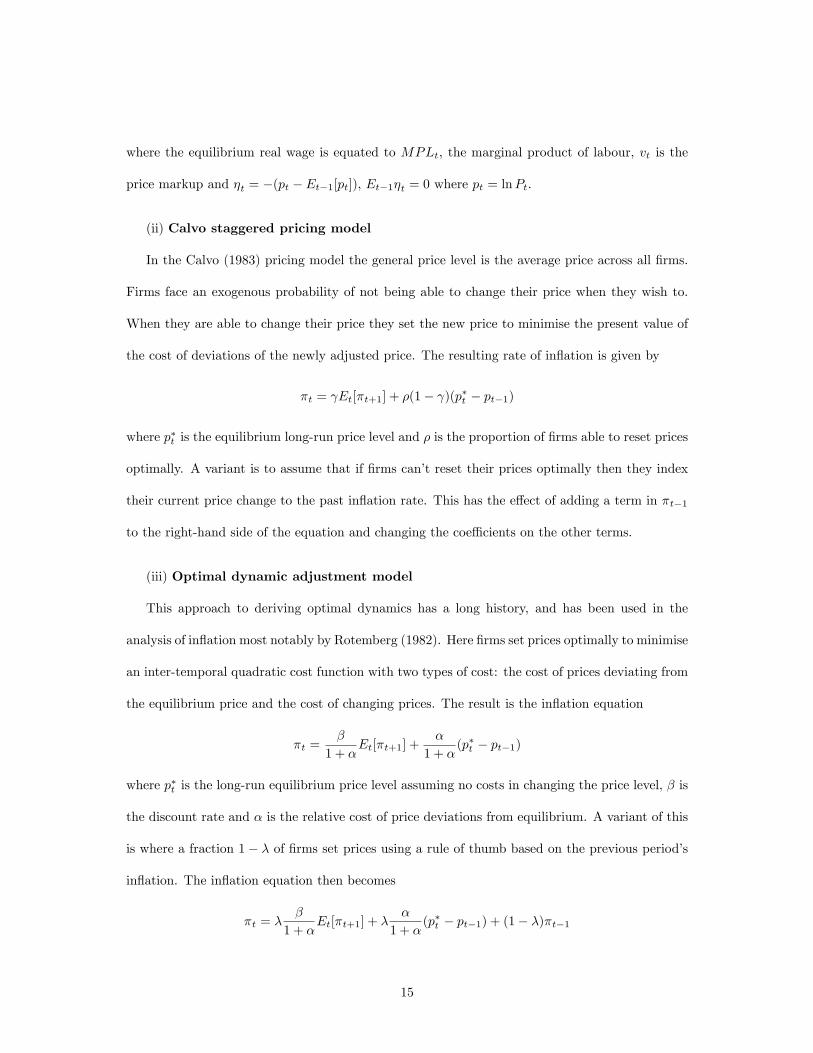
where the equilibrium real wage is equated to MPLt, the marginal product of labour, vt is the
price markup and �t = �(pt � Et�1[pt]), Et�1�t = 0 where pt = lnPt.
(ii) Calvo staggered pricing model
In the Calvo (1983) pricing model the general price level is the average price across all �rms.
Firms face an exogenous probability of not being able to change their price when they wish to.
When they are able to change their price they set the new price to minimise the present value of
the cost of deviations of the newly adjusted price. The resulting rate of in�ation is given by
�t = Et[�t+1] + �(1� )(p�t � pt�1)
where p�t is the equilibrium long-run price level and � is the proportion of �rms able to reset prices
optimally. A variant is to assume that if �rms can�t reset their prices optimally then they index
their current price change to the past in�ation rate. This has the e¤ect of adding a term in �t�1
to the right-hand side of the equation and changing the coe¢ cients on the other terms.
(iii) Optimal dynamic adjustment model
This approach to deriving optimal dynamics has a long history, and has been used in the
analysis of in�ation most notably by Rotemberg (1982). Here �rms set prices optimally to minimise
an inter-temporal quadratic cost function with two types of cost: the cost of prices deviating from
the equilibrium price and the cost of changing prices. The result is the in�ation equation
�t =�
1 + �Et[�t+1] +
�
1 + �(p�t � pt�1)
where p�t is the long-run equilibrium price level assuming no costs in changing the price level, � is
the discount rate and � is the relative cost of price deviations from equilibrium. A variant of this
is where a fraction 1� � of �rms set prices using a rule of thumb based on the previous period�s
in�ation. The in�ation equation then becomes
�t = ��
1 + �Et[�t+1] + �
�
1 + �(p�t � pt�1) + (1� �)�t�1
15

3.5 Summary
No single speci�cation emerges from this discussion, but certain features are common to most of
the models. The general form of the in�ation equation seems to be
�t = �0 + �1Et�t+1 + �2�t�1 + �4xt + �5�wt � �6� lnYtLt+ �7(�
wt +�st) + e�t (12)
where the variables retain their previous de�nitions and all coe¢ cients are expected to be positive.
Depending on the length of a period, the output gap, the rate of wage in�ation, labour productivity,
world in�ation and the change in the exchange rate may all need to be lagged. The shorter the
time period, the more likely this is. It may also be necessary to take account of the price changes
in certain non-substitutable factors such as oil. For in�ation de�ned by the GDP de�ator, it may
be possible to omit the last variable.
3.6 Two examples
To illustrate, we note two examples of the Phillips equation from the literature. Both refer to the
GDP de�ator. One is a simple marginal cost pricing model, the other has many of the features of
the more general model above.
1. Gali and Gertler (1999), Gali, Gertler and Lopez-Salido (2005)
They assume that the equilibrium price equals marginal cost, hence
p�dt = lnMCt = mct
�dt = �Et[�dt+1] + (mct � pdt ) + ��dt�1
2. Batini, Jackson and Nickell (2005)
They assume marginal cost pricing and a quadratic cost function in which the change in
16
employment is an additional cost. This gives
�dt = �Et�1[�dt+1] + Et�1(mct � pt) + �Et�1�t � �Et�1(�� lnLt+1 �� lnLt)
mct � pt = const+ sL;t + �(pmt � pt)
�t = const+ zp;t + �1xt + �2(wt � pt)
where sL;t is the share of labour, �t is the price mark-up, pmt is the price of oil, pwt is the world
price and zp;t re�ects long-term trade e¤ects.
4 The output equation
The New Keynesian output equation (2) is usually interpreted as implying that an increase in
interest rates reduces current output. The theoretical basis of this forward-looking IS function
is the consumption Euler equation in a dynamic general equilibrium model of the economy. To
illustrate we consider a simple life-cycle theory model. The problem is how to combine the Euler
equation with the household budget constraint. The method used has important consequences for
the interpretation of the e¤ect on interest rate changes on consumption, and hence output.
The representative household is assumed to maximise
Et
1Xs=0
�sU(Ct+s); � =1
1 + �
subject to the budget constraint
At+1 + Ct = Xt + (1 + rt)At
where Xt is exogenous income and At is the stock of assets held at the start of the period and rt
is their real return. (If households have net liabilities we write Bt = �At.) This gives the Euler
equation
Et[�U 0(Ct+1)
U 0(Ct)(1 + rt+1)] = 1
17
Ignoring considerations of risk (if rt is a risky return) and approximating marginal utility by
U 0(Ct+1) ' U 0(Ct) + U 00�Ct+1
gives
Et� lnCt+1 =1
�(Etrt+1 � �) (13)
where � = �CtU00
U 0 is the coe¢ cient of relative risk aversion.
In order to obtain the New Keynesian IS function (2) it is necessary to combine the Euler
equation with the household budget constraint. The common way to proceed is simply to assume
that deviations of log consumption from trend equal those of log output from its trend. This
is equivalent to assuming that the budget constraint is Ct = Yt which could be rationalised by
assuming a closed economy with no physical capital and arguing that net �nancial assets in the
economy are zero.
An alternative way is to use the following log-linear approximation to the budget constraint
A
XlnAt+1 +
C
XlnCt = lnXt + (1 + r)
A
XlnAt +
A
Xrt
where r is the average interest rate which, in general equilibrium, will be the rate of time preference
�. Equating income Xt with output Yt, and taking deviations about equilibrium, gives
yt = Etyt+1 �1
�
C
Y(Etrt+1 � �)�
A
Y[Et�
2at+2 + rat � Et�rt+1]
where at is the deviation of the logarithm of At from trend. Thus there are additional terms
compared with (2), and the coe¢ cient on the interest rate term is slightly di¤erent.
A third approach - one not usually adopted - is to derive the consumption function by solving
the budget constraint forwards. Using the log-linear approximation, the log inter-temporal budget
constraint is
EtlnAt+n(1 + r)n
+C
A
n�1Xs=0
Et lnCt+s(1 + r)s
=X
A
n�1Xs=0
Et lnXt+s(1 + r)s
+n�1Xs=0
Etrt+s(1 + r)s
+ (1 + r) lnAt
18

Taking the limit as n ! 1, assuming that limn!1lnAt+n
(1+r)n = 0 and that Etrt+s = � so that
Et lnCt+s = lnCt gives
lnCt =r
1 + r
X
C
1X0
lnXt+s(1 + r)s
+r
1 + r
A
C
n�1Xs=0
Etrt+s(1 + r)s
+ rA
ClnAt (14)
Thus log consumption depends on the expected present value of log income, on the log asset stock
and the interest rate. If households hold net liabilities then the log-linear approximation becomes
lnCt =r
1 + r
X
C
1X0
lnXt+s(1 + r)s
� r
1 + r
B
C
n�1Xs=0
Etrt+s(1 + r)s
� rBClnBt (15)
It follows that the e¤ect on consumption of an increase in interest rates depends on whether
households hold net assets or net liabilities. If households have net liabilities (Bt > 0) then
consumption, and hence output, will decrease due to the extra cost of borrowing. But if households
have net assets (At > 0) then consumption, and hence output, will increase due to the extra interest
income. For example, a tightening of current monetary policy by a one-period unit increase in
the current interest rate rt will increase lnCt by r1+r
AC if households have net assets, and decrease
lnCt by this amount if they have net liabilities, but Et lnCt+1 would be unchanged in both cases.
In other words, if households have net assets, a temporary tightening of monetary policy would be
a stimulus to the economy, not a depressive as assumed in the New Keynesian in�ation targeting
model. Since at any point of time there will be some households with net assets and others with
net liabilities, the strength of the interest rate e¤ect on consumption may be quite weak, or even
zero for a closed economy where, in the aggregate, net �nancial assets are zero.
There is a more fundamental distinction to be made in comparing this third solution with
the New Keynesian IS function. Correctly interpreted, the Euler equation says that an increase
in the expected interest rate in period t + 1 simultaneously a¤ects both current and expected
future consumption such that the expected change in consumption between periods t and t + 1
also increases. It does not say that current consumption falls as the New Keynesian IS function is
said to imply. Further, since the budget constraint must also be satis�ed, there will be a change
in asset holdings for period t+ 1.
19

To �nd out what this is, consider the e¤ect of a unit change in Etrt+1 from its initial value
of � such that interest rates in all other periods are assumed unchanged. From the consumption
functions for periods t and t + 1, with income �xed and net assets, and from the Euler equation
(13),
Et lnCt+1 � lnCt = � r
1 + r
A
Crt +
r
1 + r
A
C(1� 1
1 + r)Etrt+1 + r
A
C(Et lnAt+1 � lnAt)
=1
�(Etrt+1 � �) = 0
Hence, as a result of a unit change in Etrt+1, the change in Et lnCt+1 � lnCt is
(Et lnC�t+1 � lnC�t )� (Et lnCt+1 � lnCt) =
r
1 + r
A
C(1� 1
1 + r) + r
A
C(Et lnA
�t+1 � Et lnAt+1)
=1
�
This implies that the change in expected assets is
Et lnA�t+1 � Et lnAt+1 = �
1
�
r
(1 + r)2
A corresponding result can be derived for the case of households having net liabilities.
We conclude from this discussion of the output equation that the New Keynesian IS function
may give a completely misleading signal of the e¤ects monetary policy even to the extent of giving
the wrong sign, and that the correct way to carry out the analysis is with the consumption func-
tion. We also note that in dynamic general equilibrium models of the whole economy, additional
variables will be present in the New Keynesian IS function. This is because the national resource
constraint will re�ect the other variables in the national income identity such as government ex-
penditures and trade variables. In a full model of the economy there will also be physical capital
and in an open economy there will be a net holding of foreign assets. All of this will make the
analysis of the e¤ect of a change in interest rates more complicated. It is beyond the scope of this
paper to take this up.
20

5 Empirical evidence
We now examine empirical evidence about the NKM. We want to know how much support there is
for the standard NKM, whether less restrictive speci�cations of the in�ation and output equations
perform better, and what the estimated NKM implies for the dynamic response of in�ation to
interest rates. This evidence is based on quarterly data for the UK 1970 - 2005.
5.1 Econometric models and their estimation
The standard Phillips equation for the GDP de�ator in the NKM is a restricted version of
�dt = �0 + �1Et�dt+1 + �2�
dt�1 + �3xt + e�t
without lagged in�ation. This encompasses the alternative dynamic formulations o¤ered by the
Calvo model, the simple quadratic adjustment cost model and the Taylor model. We estimate
both the restricted version and the above equation where we employ an assumption of either rule
of thumb �rms or indexing to past in�ation as a justi�cation for the presence of lagged in�ation.
A second form of Phillips equation based on the formulation of Gali, Gertler and Lopez-Salido
(2001) is
�dt = �0 + �1Et�dt+1 + �2�
dt�1 + �3sLt + e�t
where we also make their assumption that the di¤erence between marginal costs and price is well-
measured by the wage share. A third form which aims to capture a key open economy aspect,
the potential role of import prices in the measurement of marginal cost as identi�ed by Batini,
Jackson and Nickell (2005), is
�dt = �0 + �1Et�dt+1 + �2�
dt�1 + �3sLt + �4(p
mt � pt) + e�t
The output equation has the general form
(yt � y�t ) = �0 + �1Et(yt+1 � y�t+1) + �2(yt�1 � y�t�1) + �3rt + �4(ywt � yw�t ) + eyt
21

This includes lagged dynamics in the output gap and output deviations from trend for the re-
maining G6 countries to re�ect simple open economy e¤ects. The lagged dynamics in the output
gap are consistent with the implications of habits in consumption and adjustment costs/time to
build e¤ects in investment discussed, for example, by Fuhrer and Rudebusch (2004).
The method of estimation favoured by most in this �eld is GMM with instruments drawn from
lags of the included variables plus some additional variables. Any serial correlation in the errors
e�t and eyt caused by the presence of expectational errors is assumed to be soaked up by employing
the general robust form of the covariance matrix of errors suggested by Newey and West. The
di¢ culty that this causes for our analysis is that it obscures any serial correlation caused by the
use of an incorrect form of dynamic speci�cation. We therefore adopt an alternative strategy based
on Wickens (1993) which uses two steps. Wickens shows that this method will provide consistent
estimates of the parameters and not require estimation robust to serial correlation.
1. Forecast �t and yt from lags of all of the variables, including extra variables not in the
equations but in the information set of economic agents.
2. Replace Et�t+1and Etyt+1 with the forecast for t+1 and estimate by instrumental variables
making sure not to include time t endogenous variables such as �t as instruments even though �t
is used to forecast �t+1 and yt+1.
The format of the models also allows us to employ the automatic dynamic model selection
methods (GETS) proposed by Hendry and Krolzig (2001) and reviewed in Hendry and Krolzig
(2005) (albeit in a rather di¤erent context to that discussed by those authors). Having established
the set of instrumental variables and the maximum length of the lags allowed, we allow the
automatic dynamic model selection process provided by the GETS program to choose the precise
form of the dynamics. In each case the program chooses a simpli�cation of the single lead and
multiple lags in in�ation and output, in the two equations, and the current value and lags in all
of the right hand side variables in each model. Hendry and Krolzig (2005) show that this process
of model selection is superior to the application of simple information criteria such as AIC or
22
BIC. The process ensures that the �nal model satis�es tests of misspeci�cation whilst being an
acceptable simpli�cation of the initial general unrestricted model (GUM). We provide a test of
the variable exclusion restrictions implied in the �nal model.
5.2 Estimates
In Table 1 we present the various estimates of the Phillips curve. The instruments used are: lags
1 to 5 of in�ation, output gap, labour share, real price of imports, growth of oil price, growth of
employment, real price of exports and wages.
Column 1 presents an estimate of the basic in�ation equation based on the output gap, equa-
tion (1). Both forward and backward-looking in�ation dynamics are signi�cant. The coe¢ cient
on expected future in�ation is three times the size of that of lagged in�ation and the sum of the
two is not signi�cantly di¤erent from one. The output gap has a small and insigni�cant positive
e¤ect. However, the signi�cant serial correlation and heteroskedasticity in the estimated error
makes inference unreliable. Employing the GETS technology with a maximum of four lags on
lagged in�ation and the output gap produces as �nal estimates those shown in column 2. Whilst
suggesting that the dynamics of the output gap are more complicated, the dynamics of in�ation
that emerge are like those in the basic model. Interestingly, there is no evidence of serial correla-
tion or heteroskedasticity in the errors of this equation. The test of the overidentifying restrictions
implied by the selection of included variables and instruments does not reject the equation. Like-
wise the F-test of this �nal model against the GUM is not rejected at the 10% level. In column
3 we investigate the e¤ect of restricting the speci�cation by considering a single one-year lag in
in�ation. This seems to reduce the lag in the response of in�ation to output.
23

Table 1New Keynesian Phillips Curves
tp∆ 1. 2. 3. 4. 5.
cnst. 0.0006(0.41)
0.001(0.15)
0.234(2.15)
0.396(2.07)
0.359(2.84)
1( )t tE p +∆ 0.714(6.46)
0.815(10.85)
0.649(5.98)
0.362(2.25)
0.369(4.18)
1tp −∆ 0.247(2.79)
0.187(2.14)
3tp −∆ 0.183(2.15)
4tp −∆ 0.318(4.50)
0.173(2.41)
tx 0.0193(0.268)
0.431(3.01)
1tx − 0.153(2.33)
0.589(4.44)
4tx − 0.243(2.70)
5tx − 0.183(2.15)
tsl 0.0943(2.07)
0.251(5.14)
2tsl − 0.166(3.66)
it tp p− 0.0216
(2.97)0.0996(3.96)
1 1i
t tp p− −− 0.152(5.34)
5 5i
t tp p− −− 0.028(2.51)
2R 0.568 0.699 0.636 0.574 0.768uσ 0.0101 0.00841 0.0074 0.010 0.0074
2Sargan ( )qχprob
34.2(0.36)
31.3(0.80)
FpGUM 0.0979 0.737AR (14)
prob14.06
(0.007)1.74
(0.14)8.53
(0.074)8.40
(0.078)0.326(0.86)
Heteroprob
40.67(0.00)
0.649(0.797)
11.51(0.17)
22.56(0.004)
0.846(0.64)
Estimationperiod:
1970:1 –2004:1
1976:4– 2004:1
1970:1 – 2004:1
Estimation method: Instrumental Variables
The general picture to emerge from these three sets of estimates is that the response of in�ation
to output is positive but small, and that the sum of the coe¢ cients on lag and lead in�ation is
approximately unity, which implies that there is little or no long-run tradeo¤ between in�ation
and output. Later we examine some further implications of this �nding for the NKM.
Estimation results for the marginal-cost-based Phillips curves are given in columns 4 and 5.
In column 4 a simple open economy version of the model is presented. The importance of the
forward-looking dynamics is quantitatively smaller than in the output gap-based models and the
sum of the forward and backward-looking components of the dynamics is substantially below
one. The labour share and real import price are both signi�cant and have the positive e¤ect we
expect from equation (12). Again, inference is limited by the signi�cant serial correlation and
24

heteroskedasticity that we �nd in the errors. The GETS procedure presents a somewhat di¤erent
result in this case, as shown in column 5. A much more complicated dynamic relationship emerges
from the GUM. In particular, the backward dynamics in in�ation involves in�ation with a lag
of one year. Tests of misspeci�cation favour this model over the simple version in column 4 and
an F-test supports this equation against the GUM. The sum of the coe¢ cients on lead and lag
in�ation are signi�cantly less that one, implying that there is a long-run tradeo¤ between in�ation
and output. This result is common in estimates for the UK, as for example in Batini et al (2005).
Comparison of the two types of Phillips equation suggests a number of questions about the
NKM. The output gap and a measure of marginal cost are often treated as interchangeable in
estimation. But as Gali and Gertler (1999) show, this is only possible under very restrictive
conditions, for example, that the labour market is competitive. Judging how important this is
empirically depends also on the measurement of the output gap. In our data the correlation
between the labour share and the output gap is -0.3 rather than the positive value which would
con�rm their interchangeability. An alternative to the data-generated trend output series we
employ in our output gap series is a model-based measure such as that proposed by Neiss and
Nelson (2006). The problem with their approach is that the potential output series they generate
is very volatile and therefore may not be measuring the trend that policy makers have in mind in
setting monetary policy. Perhaps further investigation of the wage markup model along the lines
proposed by Erceg, Henderson and Levin (2000) may provide a compromise estimate.
25

Table 2
New Keynesian Output Equation
tx 1. 2. 3.
cnst. 0.234(2.15)
0.0008(1.41)
0.0001(0.91)
1( )t tE x +0.610(11.9)
0.612(11.8)
0.637(10.4)
1tx −0.434(9.61)
0.371(7.03)
0.414(7.65)
1( )t t ti E p +− ∆ 0.160(3.65)
0.157(3.11)
0.156(3.68)
1 1( )t t ti E p− −− ∆ 0.148(3.75)
0.0800(1.63)
0.138(3.56)
wtx 0.0440
(2.07)2
wtx −
0.0778(2.14)
3w
tx −0.134(2.43)
4w
tx −0.0927(2.54)
2R 0.923 0.922 0.929σ 0.0035 0.0035 0.00338
2Sargan ( )qχ( )prob
51.07(0.58)
44.4(0.50)
FpGUM 0.660 0.555AR (14)
prob0.241
(0.914)4.54
(0.338)0.663
(0.619)Heteroprob
0.717(0.583)
4.41(0.353)
0.589(0.671)
Estimation period: 1976:4 2004:1Estimation method: Instrumental Variables
Estimates of the New Keynesian output equation (2) are presented in Table 2. The instruments
used are: lags 1 to 5 of in�ation, output gap, labour share, real price of imports, growth of oil
price, growth of employment, real price of exports, wages, world output gap and real interest rate
(lags 2 to 5).
In column 1 we present a closed economy model selected by GETS. This provides for rather
limited dynamics even though the GUM allowed for 4 lags in all relevant variables. The parameters
have the expected sign and size. There is little evidence against the model in any of the tests of
misspeci�cation. The signi�cance of the lagged output gap is consistent with the results in Fuhrer
(2000) and Fuhrer and Rudebusch (2004), although we also �nd that the expected future output
e¤ect continues to be important in size and signi�cance.
26

A simple generalisation of this model for the open economy is given in column 2 and a full
dynamic search employing GETS is presented in column 3. The positive e¤ect of output shocks
from overseas seems to be rather more delayed and extended over time than the simple version
suggests. This equation appears well determined with little evidence of misspeci�cation and is not
rejected as a simpli�cation of the GUM. Likewise the Sargan test provides no evidence against
the model at normal signi�cance levels. These estimates suggest that open economy e¤ects on
output are important and should not be ignored. Like the estimates of the Phillips equation, the
coe¢ cients of lag and lead terms sum to unity. We also note that the real interest rate terms have
coe¢ cients of approximately equal and opposite size. We examine the implications of these two
�ndings below.
5.3 Implications for in�ation targeting
We have seen that a common feature of the in�ation and output equations is that the sum of the
lag and lead coe¢ cients is approximately unity. This implies that the solutions have a unit root.
Further, the relative sizes of the lead and lag terms a¤ects both the form of the solution and the
sign of the impact of the other variables.
Consider the following model
yt = �Etyt+1 + (1� �)yt�1 + �xt + et
where et is an zero mean iid random variable. The presence of a unit root can be seen if the
solution is re-written as
(1� �)�yt � �Et�yt+1 = �xt + et
It follows that the model is stable or unstable depending on whether the root j �1�� j is greater or
less than unity, i.e. on whether 1 > � > 12 or 0 < � <
12 . If 1 > � >
12 the solution is non-unique
and a backward-looking model in �yt
�yt =1� ��
�yt�1 ��
�xt�1 + �x(xt � Et�1xt) + �yet �
1� ��
et�1 (16)
27

where �x and �y are arbitrary constants. If 0 < � < 12 , the solution is unique and is the forward-
looking model
�yt =�
1� ��1s=0(
�
1� � )sEtxt+s +
1
1� �et (17)
See Wickens (1993) for further details of the solution.
Now consider the output equation given by Table 2 (col. 1). This can be expressed approxi-
mately as
xt = 0:6Etxt+1 + 0:4xt�1 � 0:15�rt + ext
or as
0:4�xt = 0:6Et�xt+1 � 0:15�rt + ext
Noting that the root is greater than unity, the solution can be re-written as the non-unique
backward-looking model
�xt = 0:67�xt�1 + 0:25�rt�1 + �r(�rt � Et�1�rt) + �xext � 0:67ex;t�1
where �r and �x are arbitrary constants. Thus, due to the unit root, changes in the ouput gap
are related to changes in the interest rate. The greater the increase in the previous period�s real
interest rate, the greater the increase in the output gap. The e¤ect of an unanticipated increase
in the real interest rate at time t is not determined.
The in�ation equation (Table 1, col.3) can be written approximately as
�t = 0:24 + 0:66Et�t+1 + 0:33�t�4 � 0:5�xt + e�t
or as
��t = 0:72 + 2Et��t+1 � �3s=1��t�s � 1:5�xt + 3e�t
A rough idea of the solution may be obtained by replacing �3s=1��t�s by 3��t�1 to give
��t = 0:72 + 2Et��t+1 � 3��t�1 � 1:5�xt + 3e�t
28

or
zt = 0:24 + 0:33Etzt+1 � 0:5�xt + e�t
where zt = ��t +��t�1. From (17) this has the unique solution
��t = 0:48���t�1 � 0:5�1s=00:33sEt�xt+s + e�t
Thus, higher current and expected future increases in the output gap reduce the increase in
in�ation immediately.
Taken together, these results imply that increases in the change in interest rates will lower
the change in in�ation. Whilst this accords with the intuition of the NKM, the transmission
mechanism does not as the sign of interest rates on the output gap and of the output gap on
in�ation are the opposite to those expected.
An alternative way of examining the e¤ect of the interest rate on in�ation and output that
has the advantage of not being model dependent is through a VAR in �t, xt and it. Support for
such a VAR representation is provided by the backward-looking solution of the estimated NKM.
We obtain the following generalised impulse responses over 5 years for a VAR(8).
29

Figure 1. VAR impulse response functions
.004
.000
.004
.008
2 4 6 8 10 12 14 16 18 20
Response of LYGAP to LYGAP
.004
.000
.004
.008
2 4 6 8 10 12 14 16 18 20
Response of LYGAP to DLP
.004
.000
.004
.008
2 4 6 8 10 12 14 16 18 20
Response of LYGAP to TB3
.008
.004
.000
.004
.008
.012
2 4 6 8 10 12 14 16 18 20
Response of DLP to LYGAP
.008
.004
.000
.004
.008
.012
2 4 6 8 10 12 14 16 18 20
Response of DLP to DLP
.008
.004
.000
.004
.008
.012
2 4 6 8 10 12 14 16 18 20
Response of DLP to TB3
0.8
0.4
0.0
0.4
0.8
1.2
1.6
2 4 6 8 10 12 14 16 18 20
Response of TB3 to LYGAP
0.8
0.4
0.0
0.4
0.8
1.2
1.6
2 4 6 8 10 12 14 16 18 20
Response of TB3 to DLP
0.8
0.4
0.0
0.4
0.8
1.2
1.6
2 4 6 8 10 12 14 16 18 20
Response of TB3 to TB3
Response to Generalized One S.D. Innovations ± 2 S.E.
We observe that the responses of both in�ation and output to an interest rate shock are positive
in the short run. The response of in�ation is very weak and is insigni�cant in the short run, and
close to zero in the long run. The response of output is positive and signi�cant in the short run,
but zero in the long run. These responses are consistent with our �ndings on the properties of the
estimated New Keynesian model.
6 Conclusions
We have sought to determine whether the New Keynesian model is �t for the purpose of providing
a �nd a suitable basis for in�ation targeting in which the aim is, for example, to raise interest
rates in order to reduce in�ation. Our �ndings are not encouraging. Assuming that the standard
NKM is a correct representation of the economy, we have shown that a discretionary increase is
predicted to raise in�ation, not reduce it. In contrast, under commitment to a rule - such as a
Taylor rule - unexpectedly high interest rates are predicted to reduce in�ation.
Based on data for the UK, we have found that there is strong support for the forward-looking
30

dynamic speci�cation of the NKM. The model seems to contain a unit root with the implication
that changes in interest rates a¤ect changes in the output gap and changes in in�ation. We �nd
that the larger the increase in interest rates the smaller the change in in�ation. Whilst this accords
with the intuition of the NKM, the transmission mechanism does not as the sign of interest rates
on the output gap and of the output gap on in�ation are the opposite to those expected. Finally,
we estimated the response of in�ation to an interest shock in a three variable VAR consisting
of in�ation, the output gap and the Treasury Bill rate. We now �nd that in�ation responded
positively to interest rates.
A close analysis of the theoretical underpinnings of the NKM suggests the problem may lie in
the speci�cation of the in�ation and output equations of the NKM. In the literature most attention
has been paid to the Phillips equation. We contrast the standard Phillips equation with imperfect
competition open economy models of the equation and show that the latter have better empirical
support. An important question still to be resolved is how output a¤ects in�ation in these models.
If it is through markup e¤ect, are they via the price or the wage markup?
Perhaps more important, however, but far less considered in the literature, is the new Keynesian
IS equation. We argue that it is incorrect to base the output equation just on the Euler equation
of a DSGE model and that it is necessary to solve this together with the budget constraint or the
national resource constraint. We show that the sign of the e¤ect of an increase in interest rates
on output depends on whether households have net assets or liabilities. Only in the latter case is
the sign negative as assumed in the NKM model. Further, taking account of the national resource
constraint, implies that additional variables are required in the equation such as trade e¤ects.
Taken together, these �ndings suggest that the standard NKM does not provide a sound basis
either in theory or in the light of empirical evidence. The speci�cation of the two equations needs
much more thought and the two equations should be embedded in a somewhat more complete
model of the economy.
31

References
Ball, L. and D. Romer (1991), "Sticky prices as coordination failure", American Economic
Review, 81, 539-552.
Bank of England (1999), "The transmission mechanism of monetary policy", Bank of England
Quarterly Bulletin, 161-170.
Bank of England (2005), The Bank of England Quarterly Model.
Batini, N., B. Jackson and S. Nickell (2005), "In�ation dynamics and the labour share in the
UK", Journal of Monetary Economics, 52, 1061-1071.
Bernanke, B.S. and M. Woodford, eds, (2005), The In�ation Targeting Debate, University of
Chicago Press.
Blanchard, O. and N. Kiyotaki (1987), "Monopolistic competition and the e¤ects of aggregate
demand", American Economic Review, 77, 647-666.
Bullard, J. and K. Mitra (2002), "Learning about monetary policy rules", Journal of Monetary
Economics, 49, 1105-1129.
Calvo, G. (1983), "Staggered prices in a utility-maximising framework", Journal of Monetary
Economics, 12, 1411-1428.
Clarida, R., J. Gali and M. Gertler (1999), "The science of monetary policy: a New Keynesian
perspective", Journal of Economic Perspectives, 37, 1661-1707.
Dixit, A. and J. Stiglitz (1977), "Monopolistic competition and optimum product diversity",
American Economic Review, 67, 297-308.
Dixon, H. and N. Rankin (1994), "Imperfect competition and macroeconomics: a survey",
Oxford Economic Papers, 46, 171-199.
Erceg, C., D. Henderson and A. Levin (2000), "Optinal monetary policy with staggered wage
and price contracts", Journal of Monetary Economics, 46, 281-313.
Fuhrer, J. (2000), "Habit formation in consumption and its implications for monetary-policy
models", American Economic Review, 90, 367-90.
32

Fuhrer, J. and G. Rudebusch (2004), "Estimating the euler equation for output", Journal of
Monetary Economics 51(6), 1133-1153.
Gali, J. and M. Gertler (1999), "In�ation dynamics: a structural econometric analysis", Journal
of Monetary Economics, 44, 195-222.
Gali, J., M. Gertler and J. Lopez-Salido (2001), "European in�ation dynamics", European
Economic Review, 45, 1237-1270.
Gali, J., M. Gertler and J. Lopez-Salido (2005), "Robustness of the estimates of the hybrid
New Keynesian Phillips curve", Journal of Monetary Economics, 52, 1107-1118.
Hendry, D.F. and H-M. Krolzig (2001), Automatic Econometric Model Selection, London,
Timberlake Consultants Press.
Hendry, D.F. and H-M. Krolzig (2005), "The properties of automatic gets modelling, Economic
Journal, 115, C32�C61.
Neiss, K. and E. Nelson (2006), "In�ation dynamics, marginal cost and the output gap: evidnce
from three countries", Journal of Money Credit and Banking.
Rotemberg, J. (1982), "Sticky prices in the United States", Journal of Political Economy, 90,
1187-1211.
Taylor, J. (1979), "Staggered wage setting in a macro model", American Economic Review,
69, 108-113.
Walsh, C.E. (2003), Monetary Theory and Policy, 2nd ed., MIT Press.
Wickens, M.R. (1993), Rational expectations and integrated variables, in Essays in Economics
and Econometrics, ed J.Hall and P.C.B.Phillips, Blackwell.
Woodford, M. (2003), Interest Rates and Prices:Foundations of a Theory of Monetary Policy,
Princeton University Press.
33

Data Appendix
The data are quarterly for the UK from 1970:1 2004:1
Variables:
pt Gross Value Added De�ator (GVAD), (National Statistics: ABML/ABMM).
yt Gross value added measured at basic prices, excluding taxes less subsidies (National
Statistics: ABMM)
y�t Hodrick-Prescott trend output (�=1600).
xt = yt � y�t Output gap
slt Labour share of value added adjusted for payments to the self-employed and for general
government gross value added (National Statistics: (HAEA-NMXS)*A/(ABML-GGGVA)) where
A=(BCAJ+DYZN)/BCAJ. (Bank of England supplied)
pit Price of imports (National Statistics: IKBI/IKBL)
pwt World GDP de�ator (Bank of England data)
ywt World trade measured as G6 excluding UK GDP (Bank of England data).
nt Employment (National Statistics: BCAJ+DYZN)
wt Wages (National Statistics: (HAEA*A)/(BCAJ+DYZN)) where A=(BCAJ+DYZN)/BCAJ.
pot Price of oil : average spot price in Sterling (PETSPOT/AJFA) (Bank of England data)
xwt = ywt � yw�t World output gap : world trade minus Hodrick-Prescott trend.
it nominal 3-month treasury bill interest rate
rt = it ��pdt+1 Real interest rate
iwt World interest rate: G6 excl. UK nominal 3-month interest rate (Bank of England data)
rwt = iwt ��pwt+1 World real interest rate
All variables apart from interest rates are measured in natural logarithms.
34

www.st-and.ac.uk/cdma
ABOUT THE CDMA The Centre for Dynamic Macroeconomic Analysis was established by a direct
grant from the University of St Andrews in 2003. The Centre funds PhD students and facilitates a programme of research centred on macroeconomic theory and policy. The Centre has research interests in areas such as: characterising the key stylised facts of the business cycle; constructing theoretical models that can match these business cycles; using theoretical models to understand the normative and positive aspects of the macroeconomic policymakers' stabilisation problem, in both open and closed economies; understanding the conduct of monetary/macroeconomic policy in the UK and other countries; analyzing the impact of globalization and policy reform on the macroeconomy; and analyzing the impact of financial factors on the long-run growth of the UK economy, from both an historical and a theoretical perspective. The Centre also has interests in developing numerical techniques for analyzing dynamic stochastic general equilibrium models. Its affiliated members are Faculty members at St Andrews and elsewhere with interests in the broad area of dynamic macroeconomics. Its international Advisory Board comprises a group of leading macroeconomists and, ex officio, the University's Principal.
Affiliated Members of the School
Dr Arnab Bhattacharjee. Dr Tatiana Damjanovic. Dr Vladislav Damjanovic. Dr Laurence Lasselle. Dr Peter Macmillan. Prof Kaushik Mitra. Prof Charles Nolan (Director). Dr Gary Shea. Prof Alan Sutherland. Dr Christoph Thoenissen.
Senior Research Fellow
Prof Andrew Hughes Hallett, Professor of Economics, Vanderbilt University.
Research Affiliates
Prof Keith Blackburn, Manchester University. Prof David Cobham, Heriot-Watt University. Dr Luisa Corrado, Università degli Studi di Roma. Prof Huw Dixon, York University. Dr Anthony Garratt, Birkbeck College London. Dr Sugata Ghosh, Brunel University. Dr Aditya Goenka, Essex University. Dr Campbell Leith, Glasgow University. Dr Richard Mash, New College, Oxford. Prof Patrick Minford, Cardiff Business School. Dr Gulcin Ozkan, York University. Prof Joe Pearlman, London Metropolitan
University. Prof Neil Rankin, Warwick University. Prof Lucio Sarno, Warwick University.
Prof Eric Schaling, Rand Afrikaans University. Prof Peter N. Smith, York University. Dr Frank Smets, European Central Bank. Dr Robert Sollis, Durham University. Dr Peter Tinsley, George Washington University
and Federal Reserve Board. Dr Mark Weder, University of Adelaide.
Research Associates
Mr Nikola Bokan. Mr Michal Horvath. Ms Elisa Newby. Mr Qi Sun. Mr Alex Trew. Advisory Board
Prof Sumru Altug, Koç University. Prof V V Chari, Minnesota University. Prof John Driffill, Birkbeck College London. Dr Sean Holly, Director of the Department of
Applied Economics, Cambridge University. Prof Seppo Honkapohja, Cambridge University. Dr Brian Lang, Principal of St Andrews University. Prof Anton Muscatelli, Glasgow University. Prof Charles Nolan, St Andrews University. Prof Peter Sinclair, Birmingham University and
Bank of England. Prof Stephen J Turnovsky, Washington University. Mr Martin Weale, CBE, Director of the National
Institute of Economic and Social Research. Prof Michael Wickens, York University. Prof Simon Wren-Lewis, Exeter University.

www.st-and.ac.uk/cdma
THE CDMA CONFERENCE 2006, held in St. Andrews, 6th to the 8th of September 2006. PAPERS PRESENTED AT THE CONFERENCE, IN ORDER OF PRESENTATION:
Title Author(s) (presenter(s) in bold)
Understanding the Macroeconomics of Oil Peter Sinclair (Birminham) Caution of Activism? Monetary Policy
Strategies in an Open Economy Martin Ellison (Warwick and CEPR), Lucio Sarno (Warwick BS and CEPR) and Juoko Vilmunen (Bank of Finland)
Interest Rate Smoothing and Monetary Policy
Activism in the Bank of England, the ECB and the Fed
David Cobham (Heriot-Watt)
Linear-Quadratic Approximation, Efficiency
and Target-Implementability Paul Levine (Surrey), Joseph Pearlman (London Metropolitan) and Richard Pierse (Surrey)
The Relationship between Output and
Unemployment with Efficiency Wages Jim Malley (Glasgow) and Hassan Molana (Dundee)
Understanding Labour Market FrictionsL A
Tobin’s Q Approach Parantap Basu (Durham)
Money Velocity in an Endogenous Growth
Business Cycle with Credit Shocks Szilárd Benk (Magyar Nemzeti Bank and Central European University), Max Gillman (Cardiff and Hungarian Academy of Sciences) and Michal Kejak (CERGE-EI)
Partial Contracts Oliver Hart (Harvard) and John Hardman
Moore (Edinburgh and LSE) Optimal Fiscal Feedbak on Debt in an
Economy with Nominal Rigidities Tatiana Kirsanova (Exeter) and Simon Wren-Lewis (Exeter)
Inflation Targeting: Is the NKM fit for
purpose? Peter N. Smith (York) and Mike Wickens (York)
Testing a Simple Structural Model of
Endogenous Growth Patrick Minford (Cardiff and CEPR), David Meenagh (Cardiff) and Jiang Wang (Cardiff)
The Optimal Monetary Policy Response to
Exchange Rate Misalignments Cambell Leith (Glasgow) and Simon Wren-Lewis (Exeter)
Labor Contracts, Equal Treatment and Wage-
Unemployment Dynamics Andy Snell (Edinburgh) and Jonathan Thomas (Edinburgh)
See also the CDMA Working Paper series at www.st-andrews.ac.uk/cdma/papers.html.