Speech by

Stephen NickellBank of England Monetary Policy Committee

and London School of Economics

Two Current Monetary Policy Issues

on 16 September 2003

at a Market News International Seminar

I am most grateful to Ryan Banerjee, Giulia Faggio and Amit Kara for their assistancein the preparation of this paper. My thanks are also due to Peter Andrews,Kate Barker, Nicoletta Batini, Charles Bean, Marian Bell and Ian Bond for helpfulcomments on an earlier draft. Prepared for a Market News Seminar, 16 September2003.

1

Summary

Two Current Monetary Policy Issues

Two issues are considered, first the impending switch to targeting the HICP inflation

rate and second the implications of the steady rise in household debt. The following

is a summary of the discussion, starting with the switch to HICP targeting.

1. In the longer run, thanks to differences in computational methods and the absenceof the housing depreciation and council tax elements, the HICP inflation rate islikely, on average, to be around 0.8 pp lower than the RPI(X) inflation rate. In theshort run, the gap between the two rates is highly volatile.

2. The long-run stance of monetary policy should be gauged by the real interest rate.Since the switch from an RPIX target to an HICP target should have no long-runreal impact on the economy, the long-run stance of monetary policy will beunaffected.

3. If the HICP target is set at 2.0%, this is equivalent, in the long run, to a switchfrom an RPIX target of 2.5% to an RPIX target of 2.8%, because the long-run gapis 0.8 pp. Since the long-run real interest rate is unaffected by the switch, thelong-run nominal interest rate will be 0.3 pp higher after the switch.

4. If the HICP target is set at 2.0%, this is equivalent to a rise of 0.3 pp in the longerterm inflation rate (ie. a switch from an RPIX target of 2.5% to an RPIX target of2.8% or a switch from an HICP target of 1.7% to an HICP target of 2%, makinguse of the 0.8 pp long run gap between HICP and RPIX). This will involveslightly looser monetary policy for a limited period than would otherwise be thecase. However, given the volatility in the gap between HICP and RPIX inflationand the frequent shocks to which the economy is subject, the temporary looseningwould be barely noticeable in practice.

5. A switch to an HICP target of 2% today would have little or no impact on thecurrent stance of monetary policy despite the large gap between RPIX and HICPinflation at present. This is because this large gap is only temporary, having beengenerated by the recent surge in house price inflation which impacts on RPIX, viathe housing depreciation element, but not on HICP. As this surge fades, the gapwill close to normal levels and given the structure of the August RPIX inflationprojection, the corresponding HICP projection would not be far from 2% towardsthe end of the forecast horizon.

6. The direct inclusion of house prices in RPIX, via the housing depreciationelement, only impacted on monetary policy to the extent that the MPC was able toforecast surges in house price inflation well in advance. History indicates that itwas not able to do this. So excluding this element from the cost of living indexwill probably have little consequence for monetary policy in practice. (Of coursehouse price booms will continue to impact on monetary policy via their impact on

2

debt, consumption and aggregate demand further out. This is equally true whetherwe have an RPIX or an HICP target.)Turning next to the issue of household debt, we consider both the causes andconsequences of its dramatic increase.

7. Household secured debt (mortgages) is around 80 per cent of total household debtand is thus more significant than unsecured debt in the macroeconomic context.The secured debt to income ratio rose rapidly throughout the 1980s and from themiddle of the 1990s, so it is now more than double its level in 1980. The mostimportant factor underlying this change has been the trend increase in the numberof owner-occupied dwellings per person of working age. This trend has beengenerated by the shrinking average size of households and the increasing owner-occupation rate (strongly boosted by Council House sales). Other factors includethe somewhat higher loan-to-income ratios offered to first-time buyers in theperiod of low inflation since 1992, as mortgages are no longer heavily “front endloaded”, and the short-term burst of mortgage equity withdrawal following therecent housing boom as homeowners have greater access to the lower real interestrate borrowing available on secured debt.

8. Household unsecured debt has also risen rapidly relative to income in recentyears. By and large, this has reflected increasing debt levels per unsecured debtor,not rising numbers of unsecured debtors. A key factor explaining this is likely tohave been the rapid trend fall in unsecured borrowing rates since the late 1990s, avastly greater fall than in the Bank of England repo rate, probably due toincreasing competition in the unsecured lending market.

9. The connection between household borrowing and consumption is a tenuous one.The proportion of nominal GDP spent on household consumption was almost thesame in 2003 Q1 (63.2%) as in 1996 Q4 (62.7%) despite the vastly greater rate ofnew household borrowing in the more recent period. What has happened is thatthe rapid increase in new borrowing in recent years has been almost exactlybalanced by a rapid increase in net purchases of financial assets, a fact which israrely mentioned when household debt is discussed.

10. Looking at household balance sheets, we find that today the ratio of totalhousehold debt to total household assets (financial assets plus housing wealth) isjust below 17%, very close to its average value over the last fifteen years.Furthermore, despite the recent burst of mortgage equity withdrawal, undrawnhousing equity is rising and is now in excess of three quarters of total housingwealth. So overall, household balance sheets are relatively healthy.

11. Despite the health of average household balance sheets, there are manyhouseholds, particularly with low incomes, which are in severe difficulties withunsecured debt. The evidence on whether this situation is getting worse is mixed,but, in any event, unsecured debt is such a small proportion of the total that themacroeconomic impact of such problems is not large.

12. While the published secured debt to income ratio has been rising rapidly since1997, this is not a very helpful piece of information when it comes to analysingissues of sustainability. The problem is that the numerator of the ratio refers to the

3

sum total of mortgage debt whereas the denominator refers to the total disposableincome of all households. To be informative, the denominator should be the totaldisposable income of households with mortgages. Up-to-date data using thismeasure is unavailable but we know that the ratio of total secured debt to totalincome of secured debt holders exhibited no upward trend from 1997 to 2001.

13. Despite the above, could record levels of household debt cause seriousmacroeconomic problems in the future? There are three frequently usedarguments. The first is based on the possibility that households haveunderestimated true real interest rates. In the high inflation era prior to 1993,debts were rapidly eroded. This no longer happens and perhaps households do notfully recognise this fact. However, the young, who tend to be the most indebted(relative to their income and assets) and hence the most endangered, were notfinancially aware in the pre-1993 era, so there is little reason to think they are notmaking sensible judgments on this score. Indeed, overall, there are no strongreasons why households, or indeed lenders, should be behaving particularlyimprudently. Nor is there any persuasive evidence that they are doing so.

14. The second argument is that the economy will be a more fragile place in the futureif households have very high levels of debt. In particular, in response to a futureadverse shock, higher debt levels would lead to bigger falls in consumption and abigger economic slowdown. However, since debt service charges are the problemhere, in a higher debt world adverse shocks could be offset by a more vigorousmonetary policy response.

15. The third argument is very simple. If more people have big mortgages, a collapsein the housing market has more serious macroeconomic consequences. Of course,if this were thought to be a serious issue, one solution is a policy to reduce the sizeof the owner-occupied sector. More council houses, perhaps. But, in the presentsituation, does this mean we should use policy to discourage people from takingout mortgages? In my view, this should not be the target of monetary policy.

16. This leads to the final question, should we keep interest rates higher than would berequired to hit the inflation target in the medium term in order not to encouragefurther debt accumulation? In the light of all the previous points, my answer, atpresent, would be no.

4

1. Introduction

In recent months, two issues associated with UK monetary policy have given rise to

much debate. These are the impending switch to targeting the inflation rate of the

Harmonised Index of Consumer Prices (HICP) and the continuing anxiety associated

with the inexorable rise in household debt.

In what follows, consideration is given to both of these topics. Concerning the switch

to HICP, we look at the difference between the HICP and the RPIX measures of

inflation and then discuss the changes which would occur in the economy generally

were HICP to become the standard measure of the cost of living. We follow this by

looking at the consequences for monetary policy. We note that in the long-run, the

stance of monetary policy would be unaffected and even in the short run there would

be little noticeable difference. Finally, we consider the particular consequences

arising from the absence of any housing depreciation element in the HICP index.

Turning to the ever rising levels of household debt, we first consider why it is

increasing so fast. In this context we distinguish between secured debt (mortgages)

which is the bulk of total debt (around 80%) and unsecured debt (credit cards,

overdrafts etc). We find that the long-term increase in secured debt is driven

fundamentally by the rising number of households and the increasing proportion of

these which are owner-occupiers. Unsecured debt, on the other hand, has risen not

because of a rapid rise in the number of unsecured debtors but because of a continuing

increase in the levels of unsecured debt for each debtor, perhaps encouraged by the

rapid trend decline in interest rates on unsecured debt over the last five years.

Next we look at the relationship between rising debt and consumption, noting that in

recent years rising borrowing has, in fact, corresponded to rising rates of

accumulation of financial assets. The overall balance sheet position of households

has not been worsening rapidly. Finally, we discuss whether high levels of debt will

cause problems in the future. While there is some uncertainty here, our overall

conclusion is probably not.

5

2. The Switch to HICP

The Chancellor has announced that, at some point, the MPC will switch to an inflation

target using the HICP measure. Before looking closely at the implications of all this

for monetary policy, it is important to understand what it means for everyday

economic life.

What is the Difference between HICP and RPIX Inflation?

The main differences between the HICP and RPIX measures of inflation are as

follows.

i) In the HICP, the geometric mean is used to aggregate price changes at the

most basic level whereas the RPIX uses the arithmetic mean.

Since the geometric mean of a group of different numbers is always less than the

arithmetic mean of the same group of numbers1, this difference in the construction of

the two measures will always tend to make HICP inflation lower than RPIX inflation.

This is the formula effect and, on average, makes HICP inflation 0.5 percentage

points per annum lower than RPIX inflation.

ii) HICP excludes housing depreciation, council tax and dwellings insurance.

RPIX includes these.

The housing depreciation element and council taxes have tended to rise faster than the

other elements of RPIX, on average. Their exclusion will therefore tend, in the long

run, to lower measured inflation assuming that house prices track earnings over the

long term and council tax rates continue to rise faster than 2.5% pa. The long-run

impact of this housing effect is likely to make HICP inflation around 0.3 percentage

points per annum lower than RPIX inflation2.

iii) HICP includes university accommodation fees, foreign students tuition fees,

stockbrokers charges. RPIX excludes these. Also there are numerous other

minor differences. (The National Statistics web-site contains all the details.)

On average, these differences between HICP and RPIX contribute nothing to long-run

average inflation rate differentials between the two measures.

6

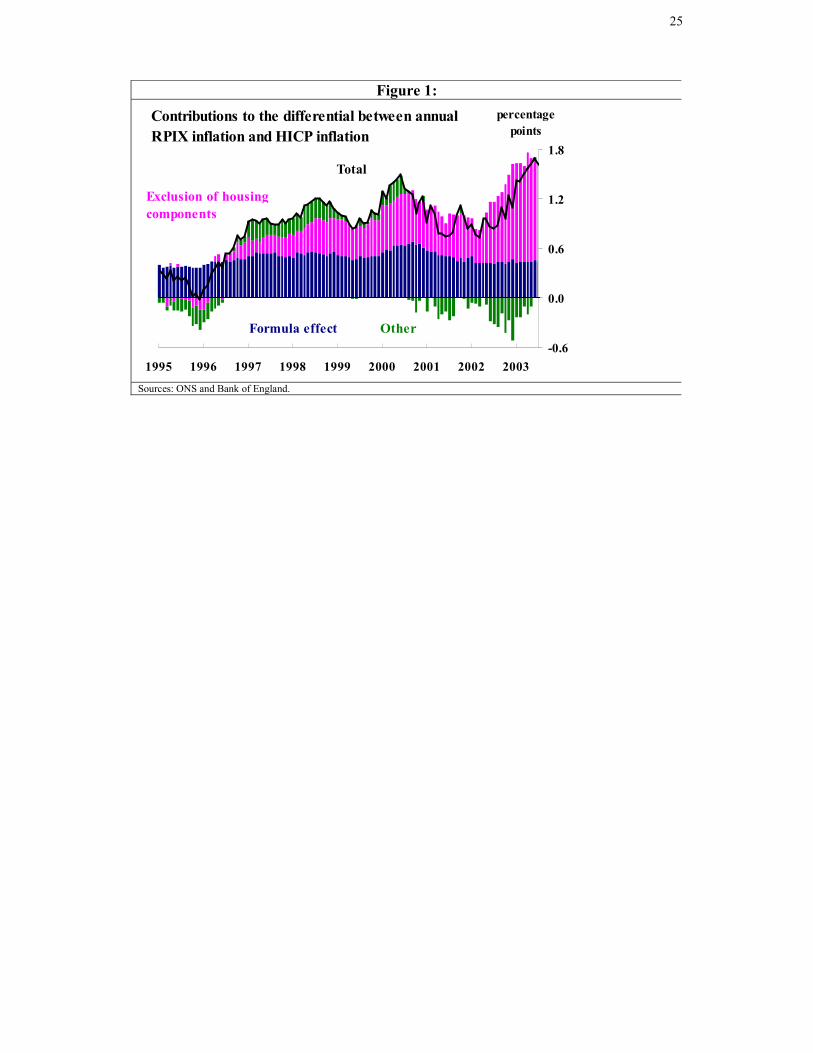
The differences under points (i) and (ii), when combined, suggest a long-run average

differential between HICP and RPIX inflation of 0.8 percentage points per annum. In

the shorter term, there is a great deal of variation in the differential as we can see from

Figure 1. While the formula effect is relatively stable, the housing and other elements

of the differential are highly volatile. Currently, the differential is very large because

the housing depreciation element, depending as it does on recent rates of house price

inflation, is making such a large contribution to RPIX inflation3. But even the long-

run average differential of 0.8 is large. So the proposed switch to the HICP measure

of inflation will mean that measured inflation will be considerably lower, on average,

than it would have been had we stuck to RPIX. So what difference will this make?

The Changes in the Economy Following a Switch to HICP

Suppose, for the sake of argument, that HICP gradually takes over from RPI(X) as the

index used in economic life. Under HICP, on average, the measured cost of living

goes up by 0.8 percentage points per annum less than under RPI(X). This change

makes no difference whatever to the rate of increase of the true cost of living, of

which HICP and RPI(X) are different measures.

So one important implication of the switch to HICP is that for given nominal wage

growth, real wage growth will be measured to be 0.8 percentage points per annum

higher after the switch. True real wage growth will, however, be unchanged. If

people understand this, they will understand that the measured increase in real wage

growth of 0.8 percentage points per annum, after the switch, is a mirage. So, for

example, if negotiations for pay increases are currently based on long-run RPIX

inflation plus x% (for productivity growth etc.), then after the switch they will have to

be based on long-run HICP inflation plus 0.8 plus x%, if they are to be unaffected by

the switch. The thing to remember is that the RPIX inflation rate and the HICP

inflation rate plus 0.8 represent the same rate of cost of living increase over the long

term.

Suppose that this does not happen. For example, suppose instead that after the switch,

unions and firms negotiate on the basis of long-run HICP inflation plus x%, where x is

the same productivity etc. effect as above. Then nominal wage growth and true real

7

wage growth will tend to be lower and this will tend to exert downward pressure on

inflation in the long run (on either measure).

Exactly as with real wage growth, the switch has the same implications for measured

real interest rates. For given nominal interest rates, after the switch to HICP,

measured (ex post) real interest rates will be, on average, 0.8 percentage points

higher. However, the true real interest rate will be unaffected. Agents in the

economy will need to get used to the fact that measured real interest rates will be

higher by roughly 0.8 percentage points, ceteris paribus. So what are the implications

of all this for monetary policy?

The Implications of the Switch to HICP for Monetary Policy

The most important point to recognise is that the long-run stance of monetary policy

should not be gauged by the nominal interest rate but by the real interest rate. And the

switch from an RPIX target to an HICP target, whatever the level of either target,

should have no long-run real impact on the economy, including on the real interest

rate. So the long-run stance of monetary policy will be unaffected. So we have,

Implication 1. The long-run stance of monetary policy will be unaffected by the

switch to an HICP target.

In order to go further, we have to make some assumption about the new target. For

the purposes of this exposition, suppose that the HICP inflation target is 2%. This is

equivalent to a long-run RPIX target of 2.8%, so it represents a genuine change to the

inflation target facing the MPC. As we have already noted, the long-run stance of

monetary policy and the true long-run real interest rate are unaffected. Since, when

measured in terms of RPIX inflation, the real interest rate will switch from (r-2.5) to

(r-2.8), where r is the nominal rate, it is obvious that to keep the real rate unchanged,

the long-run nominal rate must be 0.3 percentage points higher4. This leads to,

Implication 2. If the HICP target is set at 2.0%, this is equivalent, in the long run, to

a switch from an RPIX target of 2.5% to an RPIX target of 2.8%. Since the long-run

real interest rate is unaffected by the switch (see Implication1), the long-run nominal

interest rate will be 0.3 percentage points higher after the switch.

8

What about the consequences for monetary policy in the short run? Since the switch

involves a de facto rise in the inflation target from 2.5 to 2.8 in RPIX terms or from

1.7 to 2.0 in HICP terms, it is the job of the MPC to ensure that long-term inflation is

0.3 percentage points higher than it otherwise would have been. This involves

slightly looser monetary policy than would otherwise have been the case, for a limited

period, in order to generate the small rise in the longer-term inflation rate. However,

it would be a mistake to make too much of this. Given the large variations in the gap

between HICP inflation and RPIX inflation (see Figure 1) and the frequent shocks to

which the economy is subject, such a slight loosening of monetary policy (relative to

the counterfactual of no switch in target) would be small relative to its normal

variation. So we have,

Implication 3. If the HICP target is set at 2.0%, this implies that the short-term

monetary policy stance has to be such as to raise the longer-term inflation rate by 0.3

percentage points. This involves slightly looser monetary policy for a limited period

than would otherwise be the case. However, given the large variations in the gap

between HICP and RPIX inflation and the frequent shocks to which the economy is

subject, this temporary loosening would be barely noticeable in practice.

So far, it appears that if there were a switch to HICP with a target of 2%, this would

not make much odds. Until now, however, we have only looked at the implications of

the switch when the RPIX/HICP differential is at its long-run average level of 0.8 pp.

But today it is at around twice its long run level at 1.6 pp. What, then, would be the

consequences of the switch taking place when the gap is at a very high level? The

key point is that monetary policy decisions are based not on where inflation is today

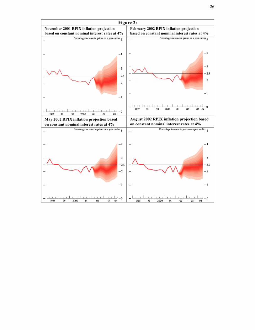
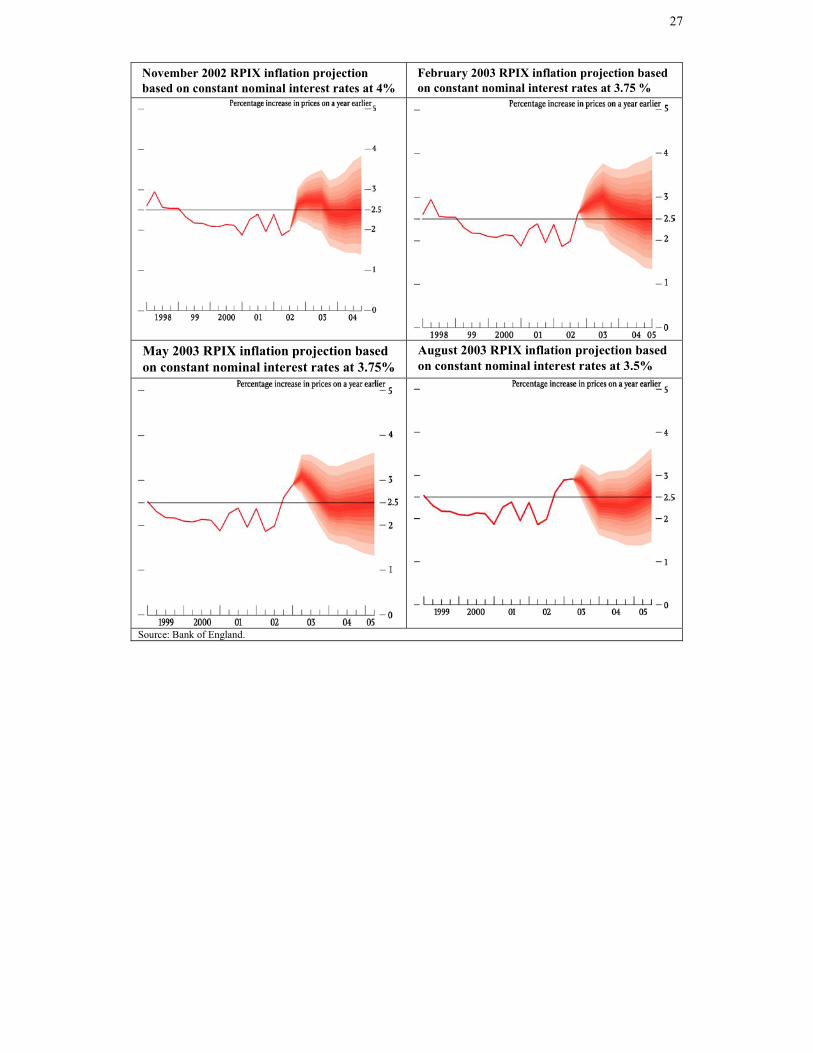
but on where inflation is expected to be a year or two hence. Looking at the RPIX

inflation projection for August 2003, (see Figure 2), the large “bump” which may be

observed stretching from the last part of 2002 to the end of 2003 is generated, in the

main, by the impact of the house price boom on RPIX inflation via the housing

depreciation component. The path of HICP inflation would not exhibit such a

"bump” and that is the main reason why the current gap is so wide as we have already

noted. But as the housing boom fades in our forecast, the bump disappears and the

RPIX/HICP gap narrows. Indeed, because the rate of house price inflation is

projected to fall below the average rate of earnings growth, the gap may well fall

below its average level of 0.8 pp. Because of this, the level of HICP inflation

9

corresponding to the RPIX projection in 2005 is not going to be very different from

2%. This implies that monetary policy decisions taken today were we using an HICP

target of 2% would probably be much the same as those we are actually taking. This

leads to,

Implication 4. A switch to an HICP target of 2% today should have little or no

impact on the current stance of monetary policy despite the large gap between RPIX

and HICP inflation. This is because this large gap is only temporary, generated by

the recent surge in house price inflation which impacts on RPIX via the housing

depreciation element but not on HICP. As this surge fades away, the gap will close to

more normal levels and given the structure of the August RPIX projection, the

corresponding HICP projection would not be very different from 2% towards the end

of the forecast horizon.

Two further implications of a switch to an HICP target are worth commenting on.

First, suppose wage setters do not follow the rules set out earlier in this section. For

example, suppose they base negotiations on long-run HICP inflation plus x. This will

tend to lead to lower nominal wage growth than we have now, lower real income

growth and ultimately downward pressure on inflation. This would then impact on

monetary policy.

The second, and perhaps more interesting, implication of the switch to an HICP target

arises from the fact that the housing depreciation element is excluded from the HICP.

We have already noted the history of this element (see Footnote 2), so what would be

the implications of its absence? The housing depreciation element in RPIX has a

weight of around 4.4% and is based on a distributed lag of the ODPM measure of

house prices. What this means is that a significant surge in house price inflation, such

as we saw in 2002, leads to a subsequent surge in RPIX inflation, such as we saw

from mid-2002. No such surge would be seen in HICP inflation. At first sight, it

might be thought that this would have a significant impact on monetary policy. In

practice, however, this would only be true if the MPC were capable of forecasting the

surge in house prices well in advance, for recall that monetary policy tends to be

influenced not by current inflation but movements in inflation which are forecast

some one to two years ahead.

10

Looking at recent history as evidenced by the recent Inflation Report projections

presented in Figure 2, the MPC completely failed to forecast the house price surge of

2002 either two years or even one year before it happened (as, incidentally, did

everyone else). The house price surge generates the “bump” in the RPIX inflation

projection in 2002/03 faintly visible in Figure 2 only from May 2002 and clearly

visible from November 2002 onwards. Consequently, by the time the surge in RPIX

inflation generated by the house price explosion was expected to come about, it was

too late to do anything about its implications for inflation. Thus, in November 2002,

the MPC expected the surge would disappear within a year and, since monetary policy

typically takes 18 months to two years to impact fully on inflation, the house price

surge had little impact on policy via its direct impact on the depreciation element of

RPIX. Of course, the house price explosion impacted strongly on monetary policy

because of its impact on debt, consumption and aggregate demand further out. But

this would have been the case even had HICP inflation been targeted. The argument

here is that the direct inclusion of house prices in the RPIX via the housing

depreciation element only impacts on monetary policy if the MPC can forecast surges

in house price inflation well in advance. Recent history indicates this is unlikely. So

excluding this element from the cost of living index will probably have little

consequence for monetary policy in practice.

2. Household Debt: Causes and Consequences

In recent months, there has been much discussion of the inexorable rise in household

debt with many dire warnings. In a relatively mild example, Philip Thornton in The

Independent (30 July, 2003) notes that,

“Britons piled on an all-time record amount of debt last month (June 2003),

triggering fears that consumers have embarked on an unsustainable borrowing binge

that will end in a crash reminiscent of the early 1990s”.

Here we look more closely at the rise in household debt, first to try and understand

why it has happened and second to look at the dangers inherent in the current position.

Why is Household Debt Rising so Rapidly?

In order to analyse household debt, it is important to distinguish between secured debt

(mortgages secured on property) and unsecured debt (credit card debt, overdrafts,

11

personal loans, hire purchase, student loans, DSS social fund loans, and others).

Around four-fifths of all household debt is secured on dwellings and so, in the

macroeconomic context, the level of secured debt is more significant. However, in

terms of personal and social problems, unsecured debt is a very important issue. Let

us consider each in turn.

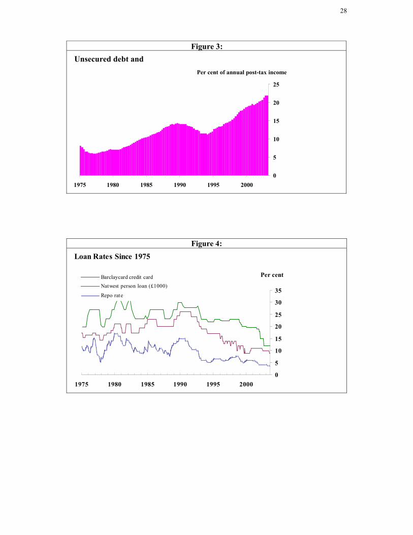
Unsecured debt. As we can see from Figure 3, unsecured debt has been rising

steadily as a proportion of total post-tax household income since the mid-1990s. By

and large, this reflects increasing debt levels per unsecured debtor, not rising numbers

of unsecured debtors5. Part of this rise may be due to the increasing ease with which

unsecured credit may be obtained, but a key factor is likely to have been the dramatic

trend fall in unsecured borrowing rates in recent years (see Figure 4). Given the

stability of inflation during this period, this represents a significant fall in real rates.

Much of this decline is unrelated to monetary policy changes, with unsecured rates

falling by far more than the repo rate in the last few years. This may have been the

consequence of increasing competition in the unsecured lending market.

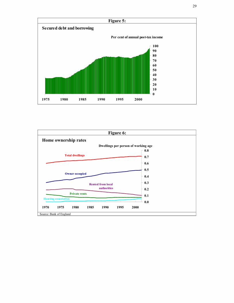
Secured debt. As we can see in Figure 5, the household secured debt to disposable

income ratio was flat in the 1970s, then rose rapidly throughout the 1980s and started

rising again in the later 1990s. So what are the driving forces behind this long-term

increase. Probably the most important factor has been the trend increase in the

number of owner-occupied dwellings per person of working age (see Figure 6). This

is partly due to the rise in the total number of occupied dwellings, reflecting smaller

households, and partly to the increasing owner occupation rate, broadly offsetting the

decline in the local authority renting sector due to council house sales. So from 1970,

the number of owner occupied dwellings per person of working age has increased by

around 75 per cent. Each new owner occupied dwelling is a potential new mortgage,

so, over the longer term, we would expect the secured debt to income ratio to rise in

the same proportion. This is because of the way the secured debt to income ratio is

measured. The numerator refers to the sum of the secured debts of all the households

with secured debt and the denominator is the sum of the disposable incomes of all

households, not just those with secured debt.

12

Interestingly, despite the fact that the number of owner occupied dwellings was rising

steadily from 1970, the debt to income ratio did not start rising until 1980. This was

because the very high rates of inflation in the 1970s were eroding real debt very

rapidly. Thus the debt to income ratios of individual mortgage holders were declining

fast enough to offset the increase in their numbers, so the aggregate debt to income

ratio remained flat. When overall inflation rates declined in the 1980s, the increase in

the number of mortgage holders began to dominate, so the aggregate secured debt to

income ratio started to rise. And, apart from a break in the early 1990s, it has been

doing so ever since. Furthermore, given that the demographic trends in Figure 6 may

be expected to continue, the rise in the secured debt to income ratio may also be

expected to continue. Indeed, even if the number of owner-occupied dwellings per

person of working age suddenly stopped increasing, because of the lags built into the

process we would expect the secured debt to income ratio to continue to rise to new

record levels for some years to come (see Hamilton, 2003 for a full analysis of all

these issues).

While these demographic factors are the key to understanding long-term trends in the

secured debt to income ratio, they are not the only ones. In a world of low inflation,

nominal interest rates are low. This means that mortgage interest and repayments are

no longer heavily “front end loaded” and so even with unchanged real interest rates,

lenders and borrowers are happy with higher initial debt to income ratios when

starting new mortgages6. So since the 1970s, we have seen a significant rise in the

income multiples allowed by mortgage lenders and a consequent rise in the average

loan to income ratios of first-time buyers. This has been reinforced by the rise over

the same period in the proportion of two-earner households. A second factor, which

is important in determining short-run fluctuations in the secured debt to income ratio,

is mortgage equity withdrawal. This always tends to rise when there is a surge in

house prices such as we have recently experienced, because, for some households,

such a surge opens up the option of further borrowing at the secured real interest rate

which still tends to be 6 percentage points or more below the unsecured rate. This

response to a lower effective real rate is entirely consistent with prudent behaviour

and does not, of itself, reflect irresponsibility on the part of either borrowers or

lenders. So having set out the forces underlying increases in household debt, we must

now look at the dangers inherent in the current situation.

13

Consumer Borrowing, Debt and Consumption

The general impression given by much of the discussion on household borrowing is

that rapidly rising debt to income ratios are inextricably linked to high rates of

household consumption growth. This is obviously wrong because households may

simply spend their borrowings on assets, not on consumption. Indeed, even when

they appear (in the data) to be spending their borrowings on consumption, they may in

fact be spending them on assets if, for example, their “consumption” consists of

buying new kitchen units. In the light of this, it is also obvious that we could observe

high levels of borrowing even when consumption growth is very depressed. So let us

look at what has been happening in recent years. Since 1997 Q4, real household

consumption growth has averaged 4.1% per annum whereas the real growth of GDP

has been 2.6% per annum. So consumption has been growing much faster than GDP

over this period. This suggests that the build-up of household debt over the same

period has been spent on consumption. Yet amazingly enough, the proportion of

nominal GDP spent on household consumption was 62.7% in 1996 Q4 and 63.2% in

2003 Q1, almost exactly the same! This despite the fact that consumption has been

growing much faster than GDP throughout the period. So how can this be?

The trick is in the prices. The price of consumption goods and services has been

rising more slowly than the price of GDP over this period. Now GDP can be thought

of as the net output of goods and services produced by the UK economy whereas

consumption is what UK households consume. Some of the output produced by the

UK economy is exported and some of the output consumed by UK households is

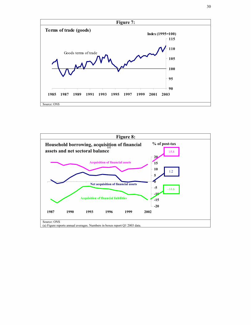
imported. And it so happens that throughout this period goods imported by the UK

have become increasingly cheaper relative to goods exported. This continuing

improvement in the terms of trade since the mid-1990s (see Figure 7) has therefore

been of continuing benefit to UK households and explains why the price of

consumption goods has grown more slowly than the price of GDP. This, in its turn,

explains how real consumption growth can be much higher than real GDP growth for

many years with barely any change in the proportion of nominal GDP being spent on

household consumption.

14

So where does the rise in household debt come into this story? In Figure 8, we see

that, by and large, the increased borrowing corresponds closely to the acquisition of

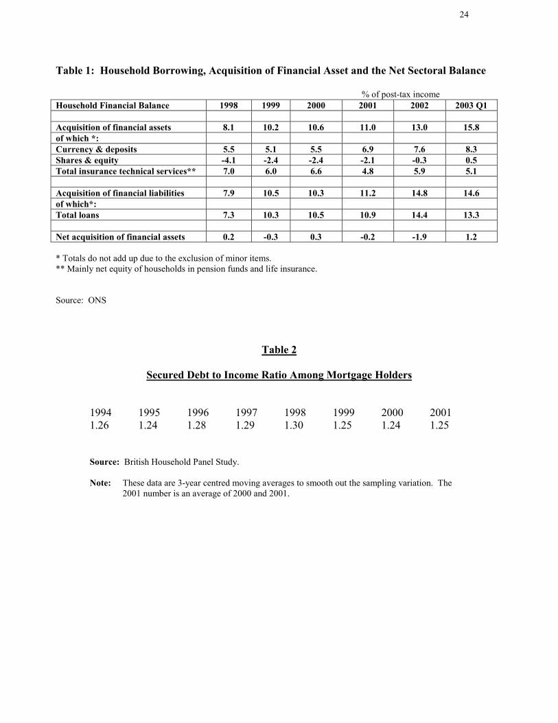
financial assets7. In Table 1, we see precisely what these assets are. Basically they

include cash and deposits as well as savings vehicles of various kinds (mainly pension

funds and life insurance). Equity flows have generally been negative. So over recent

years, the rapid increase in loans has been almost exactly balanced by a rapid increase

in the purchase of financial assets, a fact which is rarely mentioned when household

debt is discussed8. Of course, the people purchasing the assets may not be the same

people as those accumulating the liabilities. So will it all end in tears?

Is Household Debt Too High?

To answer this question, the best place to start is the overall household balance sheet

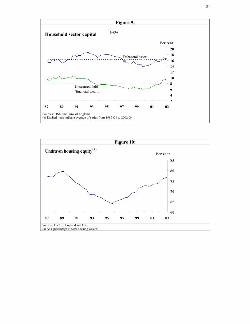
position. This is summarised in Figure 9. What we observe is that the ratio of total

household debt to total household assets (financial assets plus housing wealth) is just

below 17 per cent and is very close to its average value over the last fifteen years. So

while this ratio has risen over the last few years, mainly because of the fall in the

stock market since 2000, it is hardly at dangerous levels. Similarly, looking at the

ratio of unsecured debt to financial wealth, we see that while the number is higher

than the fifteen-year average, it is not very high by historical standards.

So while there appears to be nothing very dangerous in these overall numbers, have

the high rates of mortgage equity withdrawal produced excessive secured debt levels

relative to housing wealth? In fact, as Figure 10 makes clear, mortgage equity

withdrawal has not kept up with rising house prices, so that undrawn housing equity is

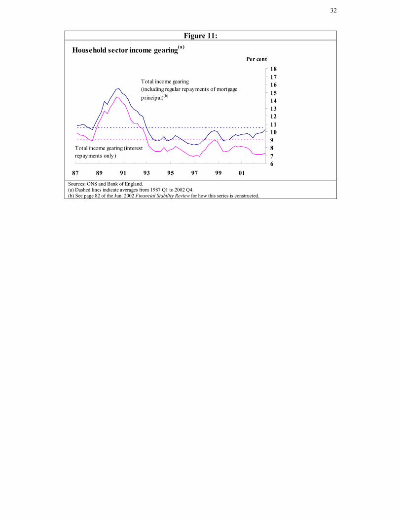
now in excess of three quarters of total housing wealth. And finally, the cost of

servicing all this household debt, even if we include regular repayments of mortgage

principal, is currently at an historically low level relative to household income (see

Figure 11). Of course, this is due to very low interest rates. But these would have to

rise to around 10 per cent to push household income gearing up to its average level in

the early 1990s.

So the overall average picture remains benign despite the rapid accumulation of debt.

And it will remain benign even if further debt is accumulated, as we expect it to be for

the reasons already discussed. But the aggregate picture may be misleading. Maybe

15

those with high debts are not the same households as those with high assets. In fact,

broadly speaking, this is not true. Almost inevitably, those with high debts tend to

have big mortgages and those with big mortgages tend to have expensive properties.

But this does not mean that debt does not cause serious problems to many households.

There are many low-income households in severe difficulty with unsecured debt. The

evidence on whether there has been an increase in these difficulties is mixed (see Cox

et al. 2002 and the Financial Stability Review, 2003, Section 2.3). But whether or not

the situation is getting worse, unsecured debt problems there are, and these are bad for

the individuals concerned and form an important issue for social policy.

Nevertheless, because the volume of unsecured debt is relatively small, this is

unlikely to be a particularly significant macroeconomic issue, so this leaves us with

the question of secured debt.

More on the secured debt picture

Any case being made for the dangers of household debt usually starts from the rising

debt to income ratio. And it is clear from Figure 5 that the secured debt to income

ratio is higher than it has ever been and, as we have seen, it is expected to go still

higher. But, as a measure of danger, or sustainability, the debt to income ratio is

almost worthless since the debt refers to the sum of the debts of debtors and the

income refers to the income of everybody. What we need in this context is the total

debt of secured debt holders (or mortgage holders) normalised on the total income of

secured debt holders. Unfortunately, it is hard to get up-to-date numbers but as we

can see from Table 2, there has been no upward trend in this ratio from the mid-1990s

to 2001. This was a period when the aggregate secured debt to income ratio rose by

around 8 percentage points. This, of course, simply reflects the fact that much of the

overall increase in debt arises from the increasing number of people with mortgages

because more and more people own their own home. It is also consistent with the fact

that in 2001 only 5 per cent of mortgage holders reported any form of distress, well

down on the levels in the early 1990s. Of course, since 2001, it is possible that

mortgage holders have seen a significant increase in debt relative to their income and

that an increased proportion of them have been imprudent. We don’t know. But such

evidence as we have, for example, historically low levels of arrears, suggests that

there is no sign that mortgage holders, who hold the vast bulk of household debt, are

facing increasing problems – indeed, lenders typically argue the reverse. More

16

sophisticated credit scoring has generated a reduction in problems. One thing we do

know, however, is that the mere existence of more mortgage debt in total does not

necessarily mean any increase in danger to the macroeconomy. And given the

historically low levels of mortgage arrears, evidence of such an increase in danger is

hard to find.

Will High Levels of Debt Cause Problems in the Future?

As we have seen, total household debt is at a record level and is highly likely to reach

even higher levels over the coming years. Despite this, household balance sheets are

not seriously stretched. Nevertheless, could these record levels of debt cause serious

macroeconomic problems in the future?

There are three distinct arguments here. The first is based on the possibility that

households have underestimated the true real interest rate which they face. So it is

sometimes argued that debtors will collectively “wake-up” to the fact that their debts

have not been eroded, and will then take fright and cut their consumption dramatically

causing severe macroeconomic problems. In the light of our previous discussion, why

households, particularly mortgage holders who have the bulk of the debt, should do

this is not at all clear. It is true that in the era of high inflation, which ended in 1992,

debts were rapidly eroded. But the mortgage holders with the highest debts relative to

income, namely the young, have no adult experience of the high inflation era.

Furthermore, they are the group with the fastest real earnings growth. So while they

might behave in the irrational fashion described above, there seems no obvious reason

why they should.

The second argument concerns the behaviour of the economy in response to shocks if

households have high, as opposed to low, levels of debt. Suppose there is a future

adverse shock to the UK economy – for example, the major European economies do

not recover. This will lead to a rise in UK unemployment and a fall in consumption

whatever the debt levels. The argument here is that higher debt levels will make

things substantially worse. That is because more people will be in a position where

they are unable to extend their borrowing. If they become unemployed, or are

threatened with unemployment, they will significantly reduce consumption because

they will be, or will have the prospect of being, unable to service their debts.

17

The first question is, will higher debt levels put substantially more people in this

position? In aggregate, there appears to be “plenty of room”. As we have seen,

secured debt is only around one quarter of gross housing wealth, a substantially lower

level than throughout the 1990s (see Figure 10). But the aggregate hides a wide

variation across the population and it is the numbers on the margin which count.

Comfort may perhaps be taken from the fact that data from the Survey of Mortgage

Lenders indicate that loan to value ratios on new mortgages are modest by historical

standards and are falling (see Financial Stability Review, June 2003, Chart 119).

Furthermore, there has been a significant demographic shift towards two earner

households over the last two decades and these households have a greater cushion

against unemployment.

Another point worth noting is that because one of the key issues in this argument is

the cost of debt service, this will be moderated by the easing of monetary policy

following the adverse shock. Back in the early 1990s, of course, this option was

unavailable because of the ERM constraint. However, the excessive debt may still

induce greater precautionary saving and a larger drop in consumption. Overall, it is

hard to tell whether higher debt levels will generate a significant additional cut back

in consumption which cannot be modified by easier monetary policy.

The third argument is very simple. More people with mortgages means more trouble

if there is a really serious collapse in the housing market. If house prices fall by 30 or

40 per cent, more people with mortgages means more people in negative equity. Of

course, the consequences of this depend to some extent on the behaviour of lenders.

If the mortgage debt continues to be treated as secured, even though some is not, then

debt service costs remain unchanged. So a lot will then depend on the collateral

damage associated with the collapse in the housing market and what caused it in the

first place. For example, the house price correction in the late 1980s and early 1990s

was basically a consequence of the 15 per cent interest rates required to control

inflation. The tight monetary policy also generated a big rise in unemployment and

all this together had a big macroeconomic impact. This particular scenario seems

unlikely today. But what causes the collapse in house prices is not the main question.

The issue is, if some disaster happens in the housing market, does the fact that more

18

people have mortgages make the consequences very much worse? So much worse,

indeed, that monetary policy should be used today to discourage individuals from

taking out mortgages. In my view, this should not be a target of monetary policy.

This leads to the final question, namely, should we keep interest rates higher than

would be required to hit the inflation target in the medium term in order not to

encourage further debt accumulation, because this will add to the risk of sharper falls

in consumption generating an even bigger undershoot of the inflation target further

out? In the light of all the previous discussion, my judgment, at present, would be no.

4. Summary and Conclusions

We have looked at two issues, first the impending switch to targeting the HICP

inflation rate and second the implications of the steady rise in household debt. The

following is a summary of the discussion, starting with the switch to HICP targeting.

1. In the longer run, thanks to differences in computational methods and the absenceof the housing depreciation and council tax elements, the HICP inflation rate islikely, on average, to be around 0.8 pp lower than the RPI(X) inflation rate. In theshort run, the gap between the two rates is highly volatile.

2. The long-run stance of monetary policy should be gauged by the real interest rate.Since the switch from an RPIX target to an HICP target should have no long-runreal impact on the economy, the long-run stance of monetary policy will beunaffected.

3. If the HICP target is set at 2.0%, this is equivalent, in the long run, to a switchfrom an RPIX target of 2.5% to an RPIX target of 2.8%, because the long-run gapis 0.8 pp. Since the long-run real interest rate is unaffected by the switch, thelong-run nominal interest rate will be 0.3 pp higher after the switch.

4. If the HICP target is set at 2.0%, this is equivalent to a rise of 0.3 pp in the longerterm inflation rate (ie. a switch from an RPIX target of 2.5% to an RPIX target of2.8% or a switch from an HICP target of 1.7% to an HICP target of 2%, makinguse of the 0.8 pp long run gap between HICP and RPIX). This will involveslightly looser monetary policy for a limited period than would otherwise be thecase. However, given the volatility in the gap between HICP and RPIX inflationand the frequent shocks to which the economy is subject, the temporary looseningwould be barely noticeable in practice.

5. A switch to an HICP target of 2% today would have little or no impact on thecurrent stance of monetary policy despite the large gap between RPIX and HICPinflation at present. This is because this large gap is only temporary, having beengenerated by the recent surge in house price inflation which impacts on RPIX, via

19

the housing depreciation element, but not on HICP. As this surge fades, the gapwill close to normal levels and given the structure of the August RPIX inflationprojection, the corresponding HICP projection would not be far from 2% towardsthe end of the forecast horizon.

6. The direct inclusion of house prices in RPIX, via the housing depreciationelement, only impacted on monetary policy to the extent that the MPC was able toforecast surges in house price inflation well in advance. History indicates that itwas not able to do this. So excluding this element from the cost of living indexwill probably have little consequence for monetary policy in practice. (Of coursehouse price booms will continue to impact on monetary policy via their impact ondebt, consumption and aggregate demand further out. This is equally true whetherwe have an RPIX or an HICP target.)Turning next to the issue of household debt, we consider both the causes andconsequences of its dramatic increase.

7. Household secured debt (mortgages) is around 80 per cent of total household debtand is thus more significant than unsecured debt in the macroeconomic context.The secured debt to income ratio rose rapidly throughout the 1980s and from themiddle of the 1990s, so it is now more than double its level in 1980. The mostimportant factor underlying this change has been the trend increase in the numberof owner-occupied dwellings per person of working age. This trend has beengenerated by the shrinking average size of households and the increasing owner-occupation rate (strongly boosted by Council House sales). Other factors includethe somewhat higher loan-to-income ratios offered to first-time buyers in theperiod of low inflation since 1992, as mortgages are no longer heavily “front endloaded”, and the short-term burst of mortgage equity withdrawal following therecent housing boom as homeowners have greater access to the lower real interestrate borrowing available on secured debt.

8. Household unsecured debt has also risen rapidly relative to income in recentyears. By and large, this has reflected increasing debt levels per unsecured debtor,not rising numbers of unsecured debtors. A key factor explaining this is likely tohave been the rapid trend fall in unsecured borrowing rates since the late 1990s, avastly greater fall than in the Bank of England repo rate, probably due toincreasing competition in the unsecured lending market.

9. The connection between household borrowing and consumption is a tenuous one.The proportion of nominal GDP spent on household consumption was almost thesame in 2003 Q1 (63.2%) as in 1996 Q4 (62.7%) despite the vastly greater rate ofnew household borrowing in the more recent period. What has happened is thatthe rapid increase in new borrowing in recent years has been almost exactlybalanced by a rapid increase in net purchases of financial assets, a fact which israrely mentioned when household debt is discussed.

10. Looking at household balance sheets, we find that today the ratio of totalhousehold debt to total household assets (financial assets plus housing wealth) isjust below 17%, very close to its average value over the last fifteen years.Furthermore, despite the recent burst of mortgage equity withdrawal, undrawn

20

housing equity is rising and is now in excess of three quarters of total housingwealth. So overall, household balance sheets are relatively healthy.

11. Despite the health of average household balance sheets, there are manyhouseholds, particularly with low incomes, which are in severe difficulties withunsecured debt. The evidence on whether this situation is getting worse is mixed,but, in any event, unsecured debt is such a small proportion of the total that themacroeconomic impact of such problems is not large.

12. While the published secured debt to income ratio has been rising rapidly since1997, this is not a very helpful piece of information when it comes to analysingissues of sustainability. The problem is that the numerator of the ratio refers to thesum total of mortgage debt whereas the denominator refers to the total disposableincome of all households. To be informative, the denominator should be the totaldisposable income of households with mortgages. Up-to-date data using thismeasure is unavailable but we know that the ratio of total secured debt to totalincome of secured debt holders exhibited no upward trend from 1997 to 2001.

13. Despite the above, could record levels of household debt cause seriousmacroeconomic problems in the future? There are three frequently usedarguments. The first is based on the possibility that households haveunderestimated true real interest rates. In the high inflation era prior to 1993,debts were rapidly eroded. This no longer happens and perhaps households do notfully recognise this fact. However, the young, who tend to be the most indebted(relative to their income and assets) and hence the most endangered, were notfinancially aware in the pre-1993 era, so there is little reason to think they are notmaking sensible judgments on this score. Indeed, overall, there are no strongreasons why households, or indeed lenders, should be behaving particularlyimprudently. Nor is there any persuasive evidence that they are doing so.

14. The second argument is that the economy will be a more fragile place in the futureif households have very high levels of debt. In particular, in response to a futureadverse shock, higher debt levels would lead to bigger falls in consumption and abigger economic slowdown. However, since debt service charges are the problemhere, in a higher debt world adverse shocks could be offset by a more vigorousmonetary policy response.

15. The third argument is very simple. If more people have big mortgages, a collapsein the housing market has more serious macroeconomic consequences. Of course,if this were thought to be a serious issue, one solution is a policy to reduce the sizeof the owner-occupied sector. More council houses, perhaps. But, in the presentsituation, does this mean we should use policy to discourage people from takingout mortgages? In my view, this should not be the target of monetary policy.

16. This leads to the final question, should we keep interest rates higher than would berequired to hit the inflation target in the medium term in order not to encouragefurther debt accumulation? In the light of all the previous points, my answer, atpresent, would be no.

21

Footnotes

1. If there are two numbers, 21 a,a , the arithmetic mean (AM) is � �21 aa21 � and the

geometric mean (GM) is � � 21

21aa . If there are n numbers n21 a,...,a,a , the AM is

� �n21 a....aan1

�� and the GM is � � n1

n321 a...aaa . So long as the numbers are all

positive and not all the same, a famous theorem in mathematics states that the GMis less than the AM. For example if 4a,1a 21 �� , the AM is � � 2412

1 �� ½ and

the GM is � � 24x1 21

� .

2. This is based on a long-run rate of house price inflation of 4.5% (in line with trendaverage earnings growth) and council tax rises of 6.5% a year (the average gapbetween council tax rises and RPIX inflation over the last seven years is around 4percentage points).

3. The housing depreciation element of RPIX is supposed to capture the contributionto the cost of living of the costs associated with maintaining homes in response totheir natural tendency to depreciate over time – eg. replacing the roof whennecessary. This element was only introduced into the RPI in 1995 as aconsequence of the majority recommendation of the RPI Advisory Committee(see CSO, 1994). This majority recommendation suggested that the costsassociated with putting right the depredations of ageing in homes was bestmeasured by a distributed lag on house prices. As the closely argued minorityview expressed by Michael Fleming, Rita Maurice and Ralph Turvey noted, therewas a serious problem here, namely that a substantial proportion of the rise in theprice of housing reflects a rise in the price of land. Since land does not depreciate,the price of housing does not accurately reflect housing depreciation costs, indeedit typically overstates them (although not always; it probably understates themwhen house prices are falling). Arguably, some index of building costs wouldprobably have been a better indicator of housing depreciation costs.

4. In terms of HICP inflation, we currently have a target which is 1.7 (2.5 less 0.8).This is moved up to 2.0 after the switch. So if r is the nominal rate, the real rateshifts from (r-1.7) to (r-2.0). If the real rate is to remain unchanged, the nominalrate must be 0.3 pp higher after the switch.

5. See Cox et al. (2002) for data up to 2000. A recent survey by NMG researchsuggests that this has remained more or less true up to 2003.

6. See Nickell (2002) for a detailed analysis.

7. Simply to clarify, household savings are equal to their net acquisition of financialassets shown in Figure 8 plus their net acquisition of real assets, basically housing.

8. This is not a new point. Robert Barrie, UK economist at CSFB is quoted in PhilipThornton’s 30 July Independent article as saying precisely this. As he notes,

22

“those who focussed on debt liabilities often forgot to mention the fact thathouseholds had also bought piles of assets”.

23

References

CSO (1994), “Treatment of Owner Occupiers’ Housing Costs in the Retail PricesIndex”, Retail Prices Index Advisory Committee, December, CM 2717(London: HMSO).

Cox, P., Whitley, J. D. and Brierley, P. G. (2002), “Financial Pressures in the UKHousehold Sector: Evidence from the British Household Panel Study”, Bankof England Quarterly Bulletin, 42(4), Winter.

Financial Stability Review (2003), Bank of England, June (Issue No.14).

Hamilton, R. (2003), “Trends in Household Aggregate Secured Debt and Borrowing”,Bank of England Quarterly Bulletin 43(3), forthcoming.

Nickell, S. (2002), “Monetary Policy Issues: Past, Present, Future”, Bank of EnglandQuarterly Bulletin, 42(3).

24

Table 1: Household Borrowing, Acquisition of Financial Asset and the Net Sectoral Balance

% of post-tax incomeHousehold Financial Balance 1998 1999 2000 2001 2002 2003 Q1

Acquisition of financial assets 8.1 10.2 10.6 11.0 13.0 15.8of which *:Currency & deposits 5.5 5.1 5.5 6.9 7.6 8.3Shares & equity -4.1 -2.4 -2.4 -2.1 -0.3 0.5Total insurance technical services** 7.0 6.0 6.6 4.8 5.9 5.1

Acquisition of financial liabilities 7.9 10.5 10.3 11.2 14.8 14.6of which*:Total loans 7.3 10.3 10.5 10.9 14.4 13.3

Net acquisition of financial assets 0.2 -0.3 0.3 -0.2 -1.9 1.2

* Totals do not add up due to the exclusion of minor items.** Mainly net equity of households in pension funds and life insurance.

Source: ONS

Table 2

Secured Debt to Income Ratio Among Mortgage Holders

1994 1995 1996 1997 1998 1999 2000 20011.26 1.24 1.28 1.29 1.30 1.25 1.24 1.25

Source: British Household Panel Study.

Note: These data are 3-year centred moving averages to smooth out the sampling variation. The2001 number is an average of 2000 and 2001.

25

Figure 1:

-0.6

0.0

0.6

1.2

1.8

1995 1996 1997 1998 1999 2000 2001 2002 2003

Contributions to the differential between annual RPIX inflation and HICP inflation

percentage points

Formula effect

Exclusion of housing components

Other

Total

Sources: ONS and Bank of England.

26

Figure 2:November 2001 RPIX inflation projection based on constant nominal interest rates at 4%

February 2002 RPIX inflation projection based on constant nominal interest rates at 4%

May 2002 RPIX inflation projection basedon constant nominal interest rates at 4%

August 2002 RPIX inflation projection basedon constant nominal interest rates at 4%

27

November 2002 RPIX inflation projection based on constant nominal interest rates at 4%

February 2003 RPIX inflation projection based on constant nominal interest rates at 3.75 %

May 2003 RPIX inflation projection based on constant nominal interest rates at 3.75%

August 2003 RPIX inflation projection based on constant nominal interest rates at 3.5%

Source: Bank of England.

28

Figure 3:

0

5

10

15

20

25

1975 1980 1985 1990 1995 2000

Per cent of annual post-tax income

Unsecured debt andi

Figure 4:

0

5

10

15

20

25

30

35

1975 1980 1985 1990 1995 2000

Barclaycard credit cardNatwest person loan (£1000)

Repo rate

Per cent

Loan Rates Since 1975

29

Figure 5:

0102030405060708090100

1975 1980 1985 1990 1995 2000

Per cent of annual post-tax income

Secured debt and borrowing

Figure 6:

0.0

0.1

0.2

0.3

0.4

0.5

0.6

0.7

0.8

1970 1975 1980 1985 1990 1995 2000

Dwellings per person of working age

Owner occupied

Total dwellings

Housing association

Private rents

Rented from localauthorities

Home ownership rates

Source: Bank of England

30

Figure 7:

90

95

100

105

110

115

1985 1987 1989 1991 1993 1995 1997 1999 2001 2003

Goods terms of trade

Index (1995=100)Terms of trade (goods)

Source: ONS

Figure 8:

-20

-15-10

-50

5

1015

20

1987 1990 1993 1996 1999 2002

Acquisition of financial assets

Acquisition of financial liabilities

Net acquisition of financial assets

% of post-taxincome

Household borrowing, acquisition of financialassets and net sectoral balance ����

���

�14.6

Source: ONS(a) Figure reports annual averages. Numbers in boxes report Q1 2003 data.

(a)

31

Figure 9:

2468101214161820

87 89 91 93 95 97 99 01 03

Per cent

Unsecured debt/financial wealth

Debt/total assets(c)

Household sector capitali

(a)(b)

Sources: ONS and Bank of England.(a) Dashed lines indicate average of series from 1987 Q1 to 2002 Q4.

Figure 10:

60

65

70

75

80

85

87 89 91 93 95 97 99 01 03

Per centUndrawn housing equity(a)

Sources: Bank of England and ONS.(a) As a percentage of total housing wealth.

32

Figure 11:

6789101112131415161718

87 89 91 93 95 97 99 01

Total income gearing (interest repayments only)

Per cent

Total income gearing(including regular repayments of mortgage principal)(b)

Household sector income gearing(a)

Sources: ONS and Bank of England.(a) Dashed lines indicate averages from 1987 Q1 to 2002 Q4.(b) See page 82 of the Jun. 2002 Financial Stability Review for how this series is constructed.