THE MULTI-ARMED BANDIT PROBLEM:AN EFFICIENT NON-PARAMETRIC SOLUTION

Hock Peng Chanstachp@nus.edu.sg

Department of Statistics and Applied ProbabilityNational University of Singapore

Abstract

Lai and Robbins (1985) and Lai (1987) provided efficient paramet-ric solutions to the multi-armed bandit problem, showing that armallocation via upper confidence bounds (UCB) achieves minimum re-gret. These bounds are constructed from the Kullback-Leibler infor-mation of the reward distributions, estimated from within a specifiedparametric family. In recent years there has been renewed interest inthe multi-armed bandit problem due to new applications in machinelearning algorithms and data analytics. Non-parametric arm alloca-tion procedures like ϵ-greedy and Boltzmann exploration were studied,and modified versions of the UCB procedure were also analyzed undera non-parametric setting. However unlike UCB these non-parametricprocedures are not efficient under parametric settings. In this paperwe propose a subsample comparison procedure that is non-parametric,but still efficient under parametric settings.

1 Introduction

Lai and Robbins (1985) provided an asymptotic lower bound for the regretin the multi-armed bandit problem, and proposed a play-the-leader strat-egy that is efficient, that is it achieves this bound. Lai (1987) showed thatallocation to the arm having the highest upper confidence bound (UCB),constructed from the Kullback-Leibler (KL) information between the esti-mated reward distributions of the arms, is efficient when the distributionsbelong to a specified exponential family. Agrawal (1995) modified UCB-Laiand showed that efficiency can still be achieved without having to know inadvance the total sample size.

Burnetas and Kalehakis (1996) extended the UCB to multi-parameterfamilies, almost showing efficiency in the natural setting of normal rewardswith unequal variances. Yakowitz and Lowe (1991) proposed non-parametricprocedures that do not make use of KL-information, suggesting logarithmicand polynomial rates of regret under finite exponential and moment condi-tions respectively.

1

Auer, Cesa-Bianchi and Fischer (2002) simplified UCB-Agrawal to UCB1,and showed that logarithmic regret is achieved when the reward distribu-tions are supported on [0,1]. They also studied the ϵ-greedy algorithm ofSutton and Barto (1998), providing finite-time upper bounds of its regret.Both UCB1 and ϵ-greedy are non-parametric in their applications and, un-like UCB-Lai or -Agrawal, are not expected to be efficient under a generalexponential family setting. Other non-parametric methods that have beenproposed include reinforcement comparison, Boltzmann exploration (Sut-ton and Barto, 1998) and pursuit (Thathacher and Sastry, 1985). Kuleshovand Precup (2014) provided numerical comparisons between UCB and thesemethods. For a description of applications to recommender systems and clin-ical trials, see Shivaswamy and Joachims (2012). The reader is also stronglyencouraged to go over Burtini, Loeppky and Lawrence (2015) for a compre-hensive survey of the methods, results and applications of the multi-armedbandit problem, developed over the past thirty years.

A strong competitor to UCB under the parametric setting is the use ofthe Bayesian method, see for example Fabius and van Zwet (1970), Berry(1972) and Kaufmann, Cappe and Garivier (2012). There is also a well-developed literature on optimization under an infinite-time discounted win-dow setting, in which allocation is to the arm maximizing a dynamic al-location (or Gittins) index, see the seminal papers by Gittins (1979) andGittins and Jones (1979), and also Berry and Fristedt (1985), Chang andLai (1987), Brezzi and Lai (2002) and Kim and Lim (2016) for more recentadvances. Another related problem is the study of the multi-armed banditwith irreversible constraints, initiated by Hu and Wei (1989).

In this paper we propose an arm allocation procedure that though non-parametric, is nevertheless efficient when the reward distributions are froman unspecified exponential family. It achieves this by comparing subsamplemeans of the leading arm with the sample means of its competitors. It isempirical in its approach, using more informative subsample means ratherthan full-sample means alone, for better decision-making. An earlier ver-sion of the subsampling strategy, known as best empirical sampled average(BESA), appeared in Baransi, Maillard and Mannor (2014). However thereare key differences in their implementation of subsampling from ours, as willbe elaborated in Section 2.2.

The layout of the paper is as follows. In Section 2 we describe thesubsample comparison strategy for allocating arms. In Section 3 we showthat the strategy is efficient for exponential families, including the setting ofnormal rewards with unequal variances. To the best of our knowledge, thisis the first instance that efficiency has been demonstrated under this two-

2

parameter setting. In Section 4 we show logarthmic regret under the moregeneral setting of Markovian rewards. In Section 5 we provide numericalcomparisons against existing methods. In Section 6 we prove the results ofSections 3 and 4.

2 Subsample comparisons

Let Yk1, Yk2, . . ., 1 ≤ k ≤ K, be the observations (or rewards) from a statis-tical population Πk. We assume here and in Section 3 that the rewards areindependent and identically distributed (i.i.d.) within each arm. We extendto Markovian rewards in Section 4. Let µk = EYkt and µ∗ = max1≤k≤K µk.Let ⌊·⌋ and ⌈·⌉ denote the greatest and least integer function respectively.

Consider a sequential procedure for selecting the population to be sam-pled at each time-stage. We refer to it as an arm allocation procedure in ac-cordance to this being the multi-armed bandit problem. Let Nk be the num-ber of observations from Πk afterN stages of sampling, henceN =

∑Kk=1Nk.

The objective is to minimize the regret

RN :=

K∑k=1

(µ∗ − µk)ENk.

The Kullback-Leibler information number between two densities f andg, with respect to a common (σ-finite) measure, is

D(f |g) = Ef [logf(Y )g(Y ) ], (2.1)

where Ef denotes expectation with respect to Y ∼ f . An arm allocationprocedure is said to converge uniformly fast if

RN = o(N ϵ) for all ϵ > 0, (2.2)

uniformly over all reward distributions lying within a specified parametricfamily.

Let fk be the density of Πk and let f∗ = fk for k such that µk = µ∗(assuming f∗ is unique). The celebrated result of Lai and Robbins (1985) isthat under (2.2) and additional regularity conditions,

lim infN→∞

RNlogN

≥∑

k:µk<µ∗

µ∗ − µkD(fk|f∗)

. (2.3)

Lai and Robbins (1985) and Lai (1987) went on to propose arm allocationprocedures that have regrets achieving the lower bound, and are hence effi-cient.

3

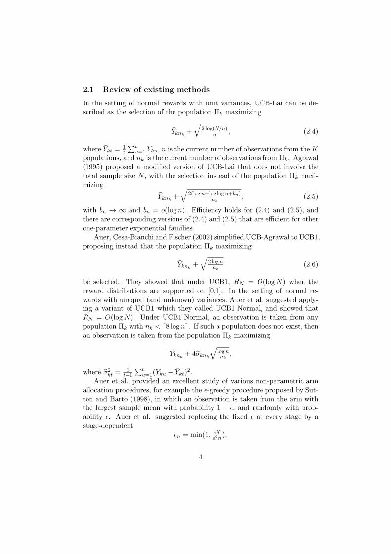
2.1 Review of existing methods

In the setting of normal rewards with unit variances, UCB-Lai can be de-scribed as the selection of the population Πk maximizing

Yknk+

√2 log(N/n)

n , (2.4)

where Ykt =1t

∑tu=1 Yku, n is the current number of observations from theK

populations, and nk is the current number of observations from Πk. Agrawal(1995) proposed a modified version of UCB-Lai that does not involve thetotal sample size N , with the selection instead of the population Πk maxi-mizing

Yknk+

√2(logn+log logn+bn)

nk, (2.5)

with bn → ∞ and bn = o(log n). Efficiency holds for (2.4) and (2.5), andthere are corresponding versions of (2.4) and (2.5) that are efficient for otherone-parameter exponential families.

Auer, Cesa-Bianchi and Fischer (2002) simplified UCB-Agrawal to UCB1,proposing instead that the population Πk maximizing

Yknk+

√2 lognnk

(2.6)

be selected. They showed that under UCB1, RN = O(logN) when thereward distributions are supported on [0,1]. In the setting of normal re-wards with unequal (and unknown) variances, Auer et al. suggested apply-ing a variant of UCB1 which they called UCB1-Normal, and showed thatRN = O(logN). Under UCB1-Normal, an observation is taken from anypopulation Πk with nk < ⌈8 log n⌉. If such a population does not exist, thenan observation is taken from the population Πk maximizing

Yknk+ 4σknk

√lognnk

,

where σ2kt =1t−1

∑tu=1(Yku − Ykt)

2.Auer et al. provided an excellent study of various non-parametric arm

allocation procedures, for example the ϵ-greedy procedure proposed by Sut-ton and Barto (1998), in which an observation is taken from the arm withthe largest sample mean with probability 1 − ϵ, and randomly with prob-ability ϵ. Auer et al. suggested replacing the fixed ϵ at every stage by astage-dependent

ϵn = min(1, cKd2n

),

4

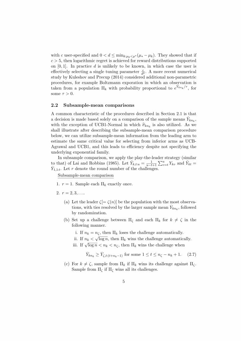
with c user-specified and 0 < d ≤ mink:µk<µ∗(µ∗ −µk). They showed that ifc > 5, then logarithmic regret is achieved for reward distributions supportedon [0, 1]. In practice d is unlikely to be known, in which case the user iseffectively selecting a single tuning parameter c

d2. A more recent numerical

study by Kuleshov and Precup (2014) considered additional non-parametricprocedures, for example Boltzmann exporation in which an observation istaken from a population Πk with probability proportional to eYknk

/τ , forsome τ > 0.

2.2 Subsample-mean comparisons

A common characteristic of the procedures described in Section 2.1 is thata decision is made based solely on a comparison of the sample means Yknk

,with the exception of UCB1-Normal in which σknk

is also utilized. As weshall illustrate after describing the subsample-mean comparison procedurebelow, we can utilize subsample-mean information from the leading arm toestimate the same critical value for selecting from inferior arms as UCB-Agrawal and UCB1, and this leads to efficiency despite not specifying theunderlying exponential family.

In subsample comparison, we apply the play-the-leader strategy (similarto that) of Lai and Robbins (1985). Let Yk,t:u = 1

u−t+1

∑uv=t Ykv and Ykt =

Y1,1:t. Let r denote the round number of the challenges.

Subsample-mean comparison

1. r = 1. Sample each Πk exactly once.

2. r = 2, 3, . . ..

(a) Let the leader ζ[= ζ(n)] be the population with the most observa-tions, with ties resolved by the larger sample mean Yknk

, followedby randomization.

(b) Set up a challenge between Πζ and each Πk for k = ζ in thefollowing manner.

i. If nk = nζ , then Πk loses the challenge automatically.

ii. If nk <√log n, then Πk wins the challenge automatically.

iii. If√log n < nk < nζ , then Πk wins the challenge when

Yknk≥ Yζ,t:(t+nk−1) for some 1 ≤ t ≤ nζ − nk + 1. (2.7)

(c) For k = ζ, sample from Πk if Πk wins its challenge against Πζ .Sample from Πζ if Πζ wins all its challenges.

5

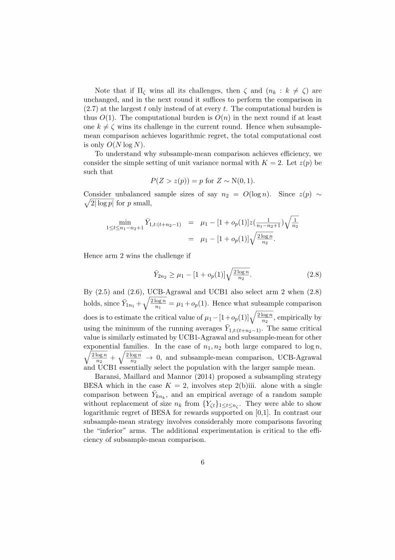
Note that if Πζ wins all its challenges, then ζ and (nk : k = ζ) areunchanged, and in the next round it suffices to perform the comparison in(2.7) at the largest t only instead of at every t. The computational burden isthus O(1). The computational burden is O(n) in the next round if at leastone k = ζ wins its challenge in the current round. Hence when subsample-mean comparison achieves logarithmic regret, the total computational costis only O(N logN).

To understand why subsample-mean comparison achieves efficiency, weconsider the simple setting of unit variance normal with K = 2. Let z(p) besuch that

P (Z > z(p)) = p for Z ∼ N(0, 1).

Consider unbalanced sample sizes of say n2 = O(log n). Since z(p) ∼√2| log p| for p small,

min1≤t≤n1−n2+1

Y1,t:(t+n2−1) = µ1 − [1 + op(1)]z(1

n1−n2+1)√

1n2

= µ1 − [1 + op(1)]√

2 lognn2

.

Hence arm 2 wins the challenge if

Y2n2 ≥ µ1 − [1 + op(1)]√

2 lognn2

. (2.8)

By (2.5) and (2.6), UCB-Agrawal and UCB1 also select arm 2 when (2.8)

holds, since Y1n1 +√

2 lognn1

= µ1+op(1). Hence what subsample comparison

does is to estimate the critical value of µ1−[1+op(1)]√

2 lognn2

, empirically by

using the minimum of the running averages Y1,t:(t+n2−1). The same criticalvalue is similarly estimated by UCB1-Agrawal and subsample-mean for otherexponential families. In the case of n1, n2 both large compared to log n,√

2 lognn2

+√

2 lognn2

→ 0, and subsample-mean comparison, UCB-Agrawal

and UCB1 essentially select the population with the larger sample mean.Baransi, Maillard and Mannor (2014) proposed a subsampling strategy

BESA which in the case K = 2, involves step 2(b)iii. alone with a singlecomparison between Yknk

, and an empirical average of a random samplewithout replacement of size nk from {Yζt}1≤t≤nζ

. They were able to showlogarithmic regret of BESA for rewards supported on [0,1]. In contrast oursubsample-mean strategy involves considerably more comparisons favoringthe “inferior” arms. The additional experimentation is critical to the effi-ciency of subsample-mean comparison.

6

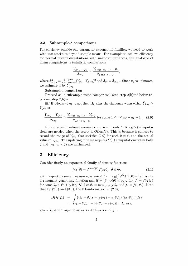
2.3 Subsample-t comparisons

For efficiency outside one-parameter exponential families, we need to workwith test statistics beyond sample means. For example to achieve efficiencyfor normal reward distributions with unknown variances, the analogue ofmean comparisons is t-statistic comparisons

Yknk− µζ

σknk

≥Yζ,t:(t+nk−1) − µζ

σζ,t:(t+nk−1),

where σ2k,t:u = 1u−t

∑uv=t(Ykv−Yk,t:u)2 and σkt = σk,1:t. Since µζ is unknown,

we estimate it by Yζnζ.

Subsample-t comparisonProceed as in subsample-mean comparison, with step 2(b)iii.′ below re-

placing step 2(b)iii.iii.′ If

√log n < nk < nζ , then Πk wins the challenge when either Yknk

≥Yζnζ

or

Yknk− Yζnζ

σknk

≥Yζ,t:(t+nk−1) − Yζnζ

σζ,t:(t+nk−1)for some 1 ≤ t ≤ nζ − nk + 1. (2.9)

Note that as in subsample-mean comparison, only O(N logN) computa-tions are needed when the regret is O(logN). This is because it suffices torecord the range of Yζnζ

that satisfies (2.9) for each k = ζ, and the actualvalue of Yζnζ

. The updating of these requires O(1) computations when bothζ and (nk : k = ζ) are unchanged.

3 Efficiency

Consider firstly an exponential family of density functions

f(x; θ) = eθx−ψ(θ)f(x; 0), θ ∈ Θ, (3.1)

with respect to some measure ν, where ψ(θ) = log[∫eθxf(x; 0)ν(dx)] is the

log moment generating function and Θ = {θ : ψ(θ) <∞}. Let fk = f(·; θk)for some θk ∈ Θ, 1 ≤ k ≤ K. Let θ∗ = max1≤k≤K θk and f∗ = f(·; θ∗). Notethat by (2.1) and (3.1), the KL-information in (2.3),

D(fk|f∗) =

∫{(θk − θ∗)x− [ψ(θk)− ψ(θ∗)]}f(x; θk)ν(dx)

= (θk − θ∗)µk − [ψ(θk)− ψ(θ∗)] = I∗(µk),

where I∗ is the large deviations rate function of f∗.

7

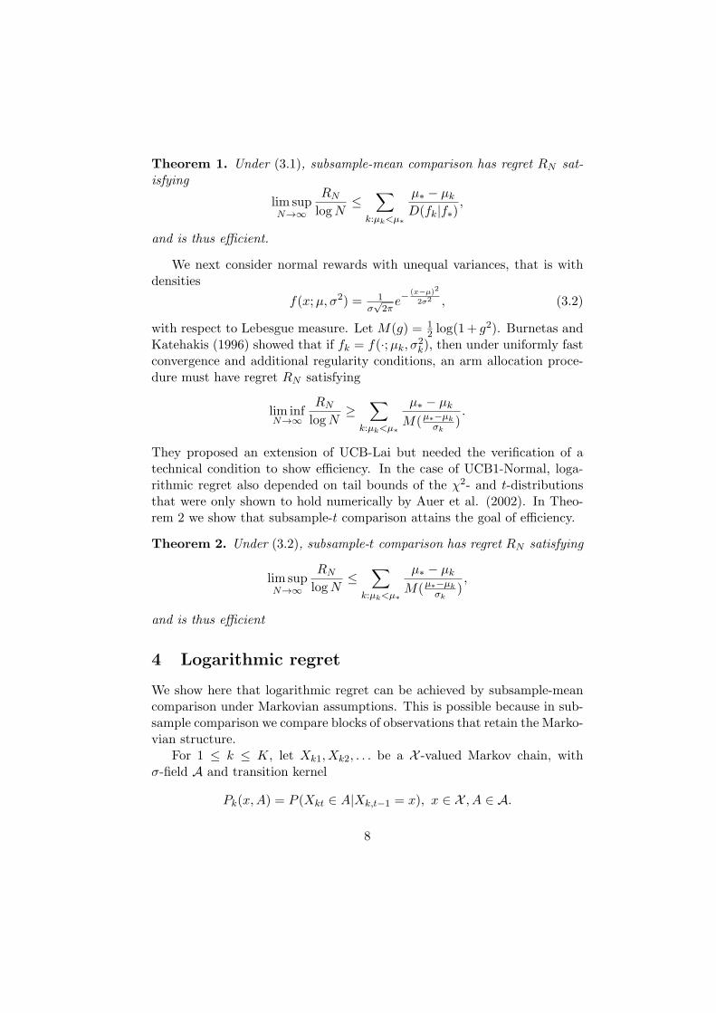
Theorem 1. Under (3.1), subsample-mean comparison has regret RN sat-isfying

lim supN→∞

RNlogN

≤∑

k:µk<µ∗

µ∗ − µkD(fk|f∗)

,

and is thus efficient.

We next consider normal rewards with unequal variances, that is withdensities

f(x;µ, σ2) = 1σ√2πe−

(x−µ)2

2σ2 , (3.2)

with respect to Lebesgue measure. Let M(g) = 12 log(1+ g2). Burnetas and

Katehakis (1996) showed that if fk = f(·;µk, σ2k), then under uniformly fastconvergence and additional regularity conditions, an arm allocation proce-dure must have regret RN satisfying

lim infN→∞

RNlogN

≥∑

k:µk<µ∗

µ∗ − µk

M(µ∗−µkσk).

They proposed an extension of UCB-Lai but needed the verification of atechnical condition to show efficiency. In the case of UCB1-Normal, loga-rithmic regret also depended on tail bounds of the χ2- and t-distributionsthat were only shown to hold numerically by Auer et al. (2002). In Theo-rem 2 we show that subsample-t comparison attains the goal of efficiency.

Theorem 2. Under (3.2), subsample-t comparison has regret RN satisfying

lim supN→∞

RNlogN

≤∑

k:µk<µ∗

µ∗ − µk

M(µ∗−µkσk),

and is thus efficient

4 Logarithmic regret

We show here that logarithmic regret can be achieved by subsample-meancomparison under Markovian assumptions. This is possible because in sub-sample comparison we compare blocks of observations that retain the Marko-vian structure.

For 1 ≤ k ≤ K, let Xk1, Xk2, . . . be a X -valued Markov chain, withσ-field A and transition kernel

Pk(x,A) = P (Xkt ∈ A|Xk,t−1 = x), x ∈ X , A ∈ A.

8

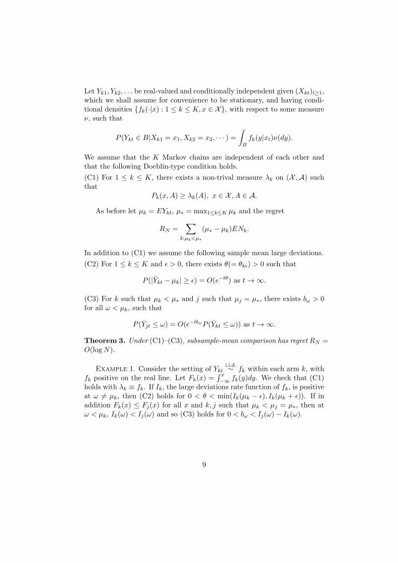
Let Yk1, Yk2, . . . be real-valued and conditionally independent given (Xkt)t≥1,which we shall assume for convenience to be stationary, and having condi-tional densities {fk(·|x) : 1 ≤ k ≤ K,x ∈ X}, with respect to some measureν, such that

P (Ykt ∈ B|Xk1 = x1, Xk2 = x2, · · · ) =∫Bfk(y|xt)ν(dy).

We assume that the K Markov chains are independent of each other andthat the following Doeblin-type condition holds.

(C1) For 1 ≤ k ≤ K, there exists a non-trival measure λk on (X ,A) suchthat

Pk(x,A) ≥ λk(A), x ∈ X , A ∈ A.

As before let µk = EYkt, µ∗ = max1≤k≤K µk and the regret

RN =∑

k:µk<µ∗

(µ∗ − µk)ENk.

In addition to (C1) we assume the following sample mean large deviations.

(C2) For 1 ≤ k ≤ K and ϵ > 0, there exists θ(= θkϵ) > 0 such that

P (|Ykt − µk| ≥ ϵ) = O(e−tθ) as t→ ∞.

(C3) For k such that µk < µ∗ and j such that µj = µ∗, there exists bω > 0for all ω < µk, such that

P (Yjt ≤ ω) = O(e−tbωP (Ykt ≤ ω)) as t→ ∞.

Theorem 3. Under (C1)–(C3), subsample-mean comparison has regret RN =O(logN).

Example 1. Consider the setting of Ykti.i.d.∼ fk within each arm k, with

fk positive on the real line. Let Fk(x) =∫ x−∞ fk(y)dy. We check that (C1)

holds with λk ≡ fk. If Ik, the large deviations rate function of fk, is positiveat ω = µk, then (C2) holds for 0 < θ < min(Ik(µk − ϵ), Ik(µk + ϵ)). If inaddition Fk(x) ≤ Fj(x) for all x and k, j such that µk < µj = µ∗, then atω < µk, Ik(ω) < Ij(ω) and so (C3) holds for 0 < bω < Ij(ω)− Ik(ω).

9

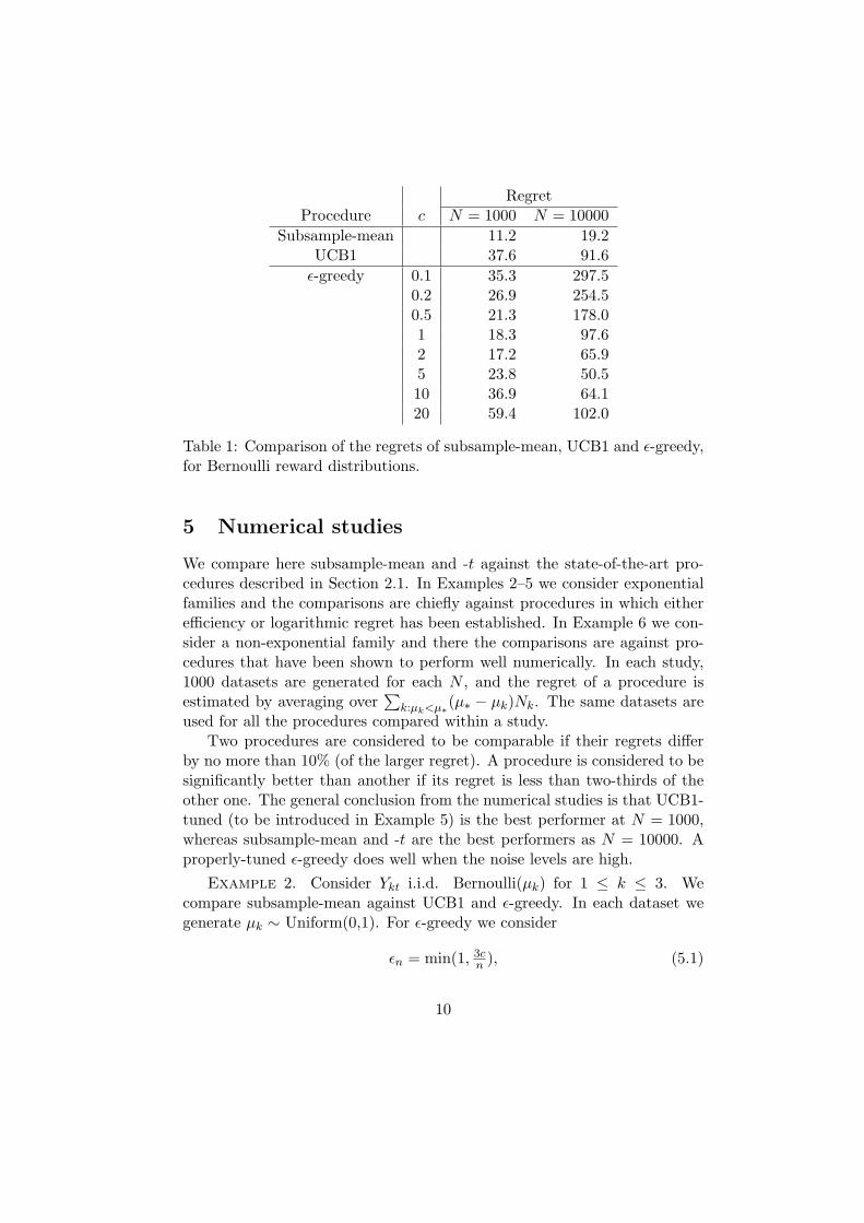
RegretProcedure c N = 1000 N = 10000

Subsample-mean 11.2 19.2UCB1 37.6 91.6

ϵ-greedy 0.1 35.3 297.50.2 26.9 254.50.5 21.3 178.01 18.3 97.62 17.2 65.95 23.8 50.510 36.9 64.120 59.4 102.0

Table 1: Comparison of the regrets of subsample-mean, UCB1 and ϵ-greedy,for Bernoulli reward distributions.

5 Numerical studies

We compare here subsample-mean and -t against the state-of-the-art pro-cedures described in Section 2.1. In Examples 2–5 we consider exponentialfamilies and the comparisons are chiefly against procedures in which eitherefficiency or logarithmic regret has been established. In Example 6 we con-sider a non-exponential family and there the comparisons are against pro-cedures that have been shown to perform well numerically. In each study,1000 datasets are generated for each N , and the regret of a procedure isestimated by averaging over

∑k:µk<µ∗

(µ∗ − µk)Nk. The same datasets areused for all the procedures compared within a study.

Two procedures are considered to be comparable if their regrets differby no more than 10% (of the larger regret). A procedure is considered to besignificantly better than another if its regret is less than two-thirds of theother one. The general conclusion from the numerical studies is that UCB1-tuned (to be introduced in Example 5) is the best performer at N = 1000,whereas subsample-mean and -t are the best performers as N = 10000. Aproperly-tuned ϵ-greedy does well when the noise levels are high.

Example 2. Consider Ykt i.i.d. Bernoulli(µk) for 1 ≤ k ≤ 3. Wecompare subsample-mean against UCB1 and ϵ-greedy. In each dataset wegenerate µk ∼ Uniform(0,1). For ϵ-greedy we consider

ϵn = min(1, 3cn ), (5.1)

10

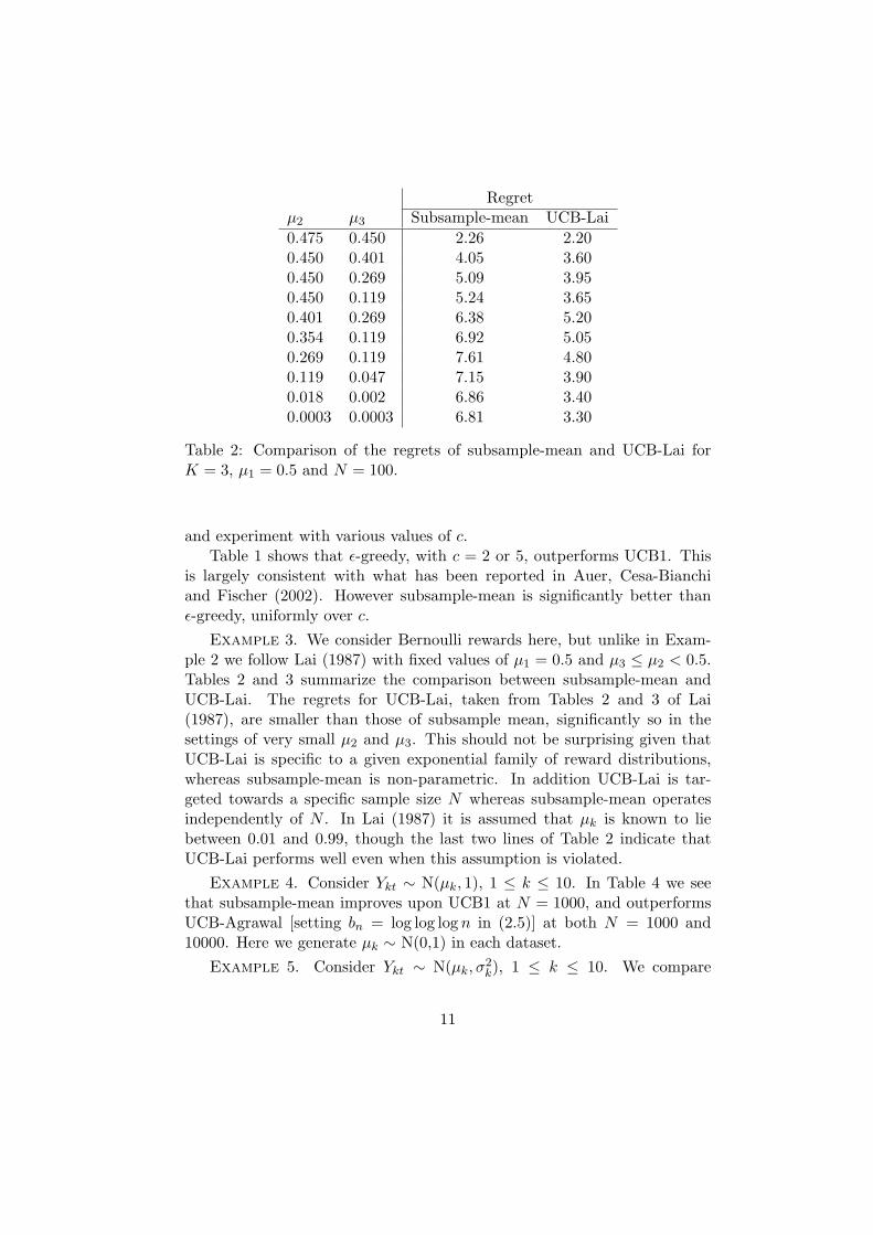
Regretµ2 µ3 Subsample-mean UCB-Lai

0.475 0.450 2.26 2.200.450 0.401 4.05 3.600.450 0.269 5.09 3.950.450 0.119 5.24 3.650.401 0.269 6.38 5.200.354 0.119 6.92 5.050.269 0.119 7.61 4.800.119 0.047 7.15 3.900.018 0.002 6.86 3.400.0003 0.0003 6.81 3.30

Table 2: Comparison of the regrets of subsample-mean and UCB-Lai forK = 3, µ1 = 0.5 and N = 100.

and experiment with various values of c.Table 1 shows that ϵ-greedy, with c = 2 or 5, outperforms UCB1. This

is largely consistent with what has been reported in Auer, Cesa-Bianchiand Fischer (2002). However subsample-mean is significantly better thanϵ-greedy, uniformly over c.

Example 3. We consider Bernoulli rewards here, but unlike in Exam-ple 2 we follow Lai (1987) with fixed values of µ1 = 0.5 and µ3 ≤ µ2 < 0.5.Tables 2 and 3 summarize the comparison between subsample-mean andUCB-Lai. The regrets for UCB-Lai, taken from Tables 2 and 3 of Lai(1987), are smaller than those of subsample mean, significantly so in thesettings of very small µ2 and µ3. This should not be surprising given thatUCB-Lai is specific to a given exponential family of reward distributions,whereas subsample-mean is non-parametric. In addition UCB-Lai is tar-geted towards a specific sample size N whereas subsample-mean operatesindependently of N . In Lai (1987) it is assumed that µk is known to liebetween 0.01 and 0.99, though the last two lines of Table 2 indicate thatUCB-Lai performs well even when this assumption is violated.

Example 4. Consider Ykt ∼ N(µk, 1), 1 ≤ k ≤ 10. In Table 4 we seethat subsample-mean improves upon UCB1 at N = 1000, and outperformsUCB-Agrawal [setting bn = log log log n in (2.5)] at both N = 1000 and10000. Here we generate µk ∼ N(0,1) in each dataset.

Example 5. Consider Ykt ∼ N(µk, σ2k), 1 ≤ k ≤ 10. We compare

11

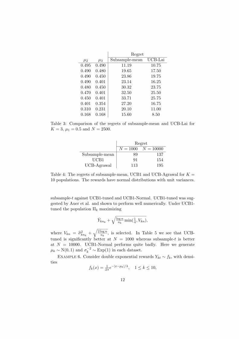
Regretµ2 µ3 Subsample-mean UCB-Lai

0.495 0.490 11.19 10.750.490 0.480 19.65 17.500.490 0.450 23.86 19.750.490 0.401 23.14 16.250.480 0.450 30.32 23.750.470 0.401 32.50 25.500.450 0.401 33.71 25.750.401 0.354 27.20 16.750.310 0.231 20.10 11.000.168 0.168 15.60 8.50

Table 3: Comparison of the regrets of subsample-mean and UCB-Lai forK = 3, µ1 = 0.5 and N = 2500.

RegretN = 1000 N = 10000

Subsample-mean 89 137UCB1 91 154

UCB-Agrawal 113 195

Table 4: The regrets of subsample-mean, UCB1 and UCB-Agrawal for K =10 populations. The rewards have normal distributions with unit variances.

subsample-t against UCB1-tuned and UCB1-Normal. UCB1-tuned was sug-gested by Auer et al. and shown to perform well numerically. Under UCB1-tuned the population Πk maximizing

Yknk+

√lognnk

min(14 , Vkn),

where Vkn = σ2knk+

√2 lognnk

, is selected. In Table 5 we see that UCB-

tuned is significantly better at N = 1000 whereas subsample-t is betterat N = 10000. UCB1-Normal performs quite badly. Here we generateµk ∼ N(0, 1) and σ−2

k ∼ Exp(1) in each dataset.

Example 6. Consider double exponential rewards Ykt ∼ fk, with densi-ties

fk(x) =12λe

−|x−µk|/λ, 1 ≤ k ≤ 10,

12

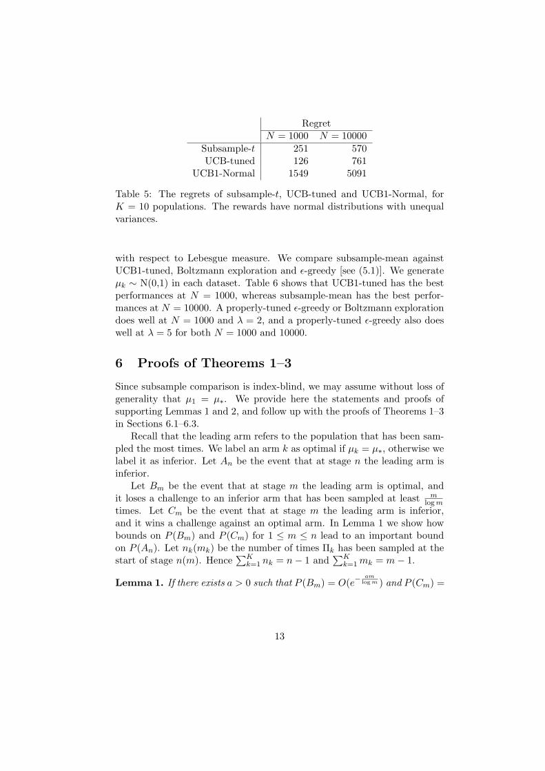
RegretN = 1000 N = 10000

Subsample-t 251 570UCB-tuned 126 761

UCB1-Normal 1549 5091

Table 5: The regrets of subsample-t, UCB-tuned and UCB1-Normal, forK = 10 populations. The rewards have normal distributions with unequalvariances.

with respect to Lebesgue measure. We compare subsample-mean againstUCB1-tuned, Boltzmann exploration and ϵ-greedy [see (5.1)]. We generateµk ∼ N(0,1) in each dataset. Table 6 shows that UCB1-tuned has the bestperformances at N = 1000, whereas subsample-mean has the best perfor-mances at N = 10000. A properly-tuned ϵ-greedy or Boltzmann explorationdoes well at N = 1000 and λ = 2, and a properly-tuned ϵ-greedy also doeswell at λ = 5 for both N = 1000 and 10000.

6 Proofs of Theorems 1–3

Since subsample comparison is index-blind, we may assume without loss ofgenerality that µ1 = µ∗. We provide here the statements and proofs ofsupporting Lemmas 1 and 2, and follow up with the proofs of Theorems 1–3in Sections 6.1–6.3.

Recall that the leading arm refers to the population that has been sam-pled the most times. We label an arm k as optimal if µk = µ∗, otherwise welabel it as inferior. Let An be the event that at stage n the leading arm isinferior.

Let Bm be the event that at stage m the leading arm is optimal, andit loses a challenge to an inferior arm that has been sampled at least m

logmtimes. Let Cm be the event that at stage m the leading arm is inferior,and it wins a challenge against an optimal arm. In Lemma 1 we show howbounds on P (Bm) and P (Cm) for 1 ≤ m ≤ n lead to an important boundon P (An). Let nk(mk) be the number of times Πk has been sampled at thestart of stage n(m). Hence

∑Kk=1 nk = n− 1 and

∑Kk=1mk = m− 1.

Lemma 1. If there exists a > 0 such that P (Bm) = O(e− am

logm ) and P (Cm) =

13

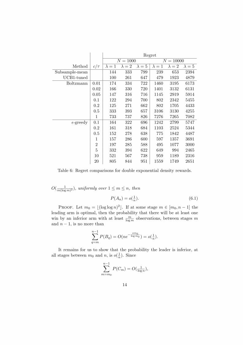
RegretN = 1000 N = 10000

Method c/τ λ = 1 λ = 2 λ = 5 λ = 1 λ = 2 λ = 5

Subsample-mean 144 333 799 239 653 2394UCB1-tuned 100 261 647 479 1923 4879

Boltzmann 0.01 174 334 722 1460 3195 61730.02 166 330 720 1401 3132 61310.05 147 316 716 1145 2919 59140.1 122 294 700 802 2342 54550.2 125 271 662 802 1705 44330.5 333 393 657 3106 3130 42551 733 737 826 7276 7265 7082

ϵ-greedy 0.1 164 322 696 1242 2799 57470.2 161 318 684 1103 2524 53440.5 152 278 638 775 1842 44871 157 286 600 597 1357 36912 197 285 588 495 1077 30005 332 394 622 649 994 246510 521 567 738 959 1189 231620 805 844 951 1559 1749 2651

Table 6: Regret comparisons for double exponential density rewards.

O( 1m(logm)2

), uniformly over 1 ≤ m ≤ n, then

P (An) = o( 1n). (6.1)

Proof. Let m0 = ⌊(log log n)2⌋. If at some stage m ∈ [m0, n − 1] theleading arm is optimal, then the probability that there will be at least onewin by an inferior arm with at least m

logm observations, between stages mand n− 1, is no more than

n−1∑q=m

P (Bq) = O(ne− am0

logm0 ) = o( 1n).

It remains for us to show that the probability the leader is inferior, atall stages between m0 and n, is o( 1n). Since

n−1∑m=m0

P (Cm) = O( 1logn),

14

the probability that an inferior leading arm wins at least n√logn

times be-

tween stages m0 and n − 1, against optimal arms, is√lognn O( 1

logn) = o( 1n).But it is not possible to have inferior leading arms at all stages between mto n, with them winning no more than n√

logntimes against optimal arms

between stagesm and n−1. This is because maxk:µk<µ∗ mk−maxk:µk=µ∗ mk

reduces by 1 after each round in which the leading inferior arm loses to alloptimal arms. Note in particular that by step 2(b)i., the leading inferiorarm wins against all inferior arms with the same number of observations.With that we conclude (6.1). ⊓⊔

Let Bnk be the event that at stage n the leading arm is optimal, and itloses a challenge to an inferior arm k.

Lemma 2. Consider the following conditions for an inferior arm k.

(I) There exists ξk > 0 such that for all ϵ > 0, as N → ∞,

P (Bnk occurs for some 1 ≤ n ≤ N with nk = ⌊(1 + ϵ)ξk logN⌋) → 0.

(II) There exists Jk > 0 such that as N → ∞,

P (Bnk occurs for some 1 ≤ n ≤ N with nk = ⌊Jk logN⌋) = O(N−1).

If (6.1), (I) and (II) hold, then

lim supN→∞

ENk

logN≤ ξk. (6.2)

Proof. By (6.1),∑N

n=1 P (An) = o(logN), and (6.2) thus follows from(I) and (II). ⊓⊔

6.1 Proof of Theorem 1

We consider here subsample-mean comparisons. Let Ij be the large devia-tions rate function of fj . By Lemmas 1 and 2 it suffices, in Lemmas 3–5 below, to verify the conditions needed to show that (6.2) holds withξk = 1/I1(µk).

Lemma 3. Under (3.1), P (Bm) = O(e− am

logm ) for some a > 0.

Proof. Consider the case that at stage m the leading optimal arm isarm 1, and it loses a challenge to an inferior arm k with mk ≥ m

logm . Letmaxj:µj<µ1 µj < ω < µ1. It follows from large deviations that

P (Y1,t:(t+mk−1) ≤ ω for some 1 ≤ t ≤ m) ≤ me−mkI1(ω),

15

P (Ykmk≥ ω) ≤ e−mkIk(ω).

Since mk ≥ mlogm , the above inequalities imply that Lemma 3 holds for

0 < a < min1≤k≤K Ik(ω). ⊓⊔

Lemma 4. Under (3.1), P (Cm) = O( 1m(logm)2

).

Proof. Consider the case that k is the leading inferior arm, and itwins a challenge against optimal arm 1 at stage m. By step 2(b)ii., arm kloses automatically when m1 <

√logm, hence we need only consider m1 >√

logm.Case 1: m1 > (logm)2. Let µk < ω < µ1. By large deviations,

P (Y1m1 < ω for some m1 > (logm)2) = O( 1m(logm)2

), (6.3)

P (Ykm1 > ω for some m1 > (logm)2) = O( 1m(logm)2

). (6.4)

Case 2:√logm < m1 < (logm)2. Since mk ≥ m−1

K , it suffices to showthat there exists ω such that

P (Y1m1 < ω) = O( 1m(logm)4

), (6.5)

P (Yk,t:(t+m1−1) > ω for 1 ≤ t ≤ m−1K −m1 + 1) (6.6)

(≤ [P (Ykm1 > ω)][(m−1)/K−m1+1]/m1) = O( 1m(logm)4

).

Since θ1 > θk, if∑m1

t=1 yt ≤ m1µk, then by (3.1),

m1∏t=1

f(yt; θ1) = e(θ1−θk)∑m1

t=1 yt−m1[ψ(θ1)−ψ(θk)]m1∏t=1

f(yt; θk)

≤ e−m1I1(µk)m1∏t=1

f(yt; θk).

Hence if ω ≤ µk, then as m1 >√logm,

P (Y1m1 < ω) ≤ e−m1I1(µk)P (Ykm1 < ω) = O( 1(logm)8

P (Ykm1 < ω)). (6.7)

Let ω(≤ µk for large m) be such that

P (Ykm1 < ω) ≤ (logm)4

m ≤ P (Ykm1 ≤ ω). (6.8)

We check that (6.5) follows from (6.7) and the first inequality in (6.8),whereas (6.6) follows from the second inequality in (6.8) and m1 ≤ (logm)2.Lemma 3 follows from (6.3)–(6.6). ⊓⊔

16

Lemma 5. Under (3.1), both (I) and (II), in the statement of Lemma 2,hold for ξk = 1/I1(µk).

Proof. Consider an inferior arm k and stage n with nk = ⌊[(1 +ϵ) logN ]/I1(µk)⌋. Let µk < ω < µ1 be such that (1 + ϵ)I1(ω) > I1(µk).It follows from large deviations that

P (Y1,t:(t+nk−1) ≤ ω for some 1 ≤ t ≤ N) ≤ Ne−nkI1(ω) → 0,

P (Yknk≥ ω) ≤ e−nkIk(ω) → 0,

and (I) therefore holds.Next consider Jk > max( 1

Ik(ω), 2I1(ω)

). If nk = ⌊Jk logN⌋, then

P (Y1,t:(t+nk−1) ≤ ω for some 1 ≤ t ≤ N) ≤ Ne−nkI1(ω) = O(N−1),

P (Yknk≥ ω) ≤ e−nkIk(ω) = O(N−1),

and (II) holds as well. ⊓⊔

6.2 Proof of Theorem 2

We consider here subsample-t comparisons. By Lemmas 1 and 2 it suffices,in Lemmas 6–8 below, to verify the conditions needed to show that (6.2)holds with ξk = 1/M(µ∗−µkσk

). Let Φ(z) = P (Z > z) for Z ∼ N(0,1).

Lemma 6. Under (3.2), P (Bm) = O(eam

logm ) for some a > 0.

Proof. Consider the case that at stage m the leading optimal arm isarm 1, and that it loses a challenge to an inferior arm k with mk ≥ m

logm .

Let ϵ > 0 be such that ω := µk−µ1+ϵ2σk

< 0, noting that

P (Ykmk

−Y1m1

σkmk≥ ω) ≤ P (

Ykmk−Y1m1

2σk≥ ω) + P (σkmk

≥ 2σk). (6.9)

Since Ykmk− Y1m1 ∼ N(µk − µ1,

σ21

m1+

σ2k

mk) and m1 ≥ mk,

P (Ykmk

−Y1mk2σk

≥ ω) ≤ Φ(ϵ√

mk

σ21+σ

2k) (6.10)

= O(m−2e− am

logm ) for 0 < a < ϵ2

2(σ21+σ

2k).

Since mk ≥ mlogm , by large deviations,

P (σkmk> 2σk) = O(m−2e

− amlogm ) for some a > 0. (6.11)

17

It follows from arguments similar to those in (6.10) and (6.11) that

P (Y1,t:(t+mk−1)−Y1m1

σ1,t:(t+mk−1)≤ ω for some 1 ≤ t ≤ m) (6.12)

≤ m[P (Y1mk

−Y1m1

σ1/2≤ ω) + P (σ1mk

≤ σ12 )]

= O(m−2e− am

logm ) for some a > 0.

It also follows from large deviations arguments that

P (Ykmk≥ Y1m1) = O(m−2e

− amlogm ) for some a > 0,

and Lemma 6 thus follows from (6.9)–(6.12). ⊓⊔

Lemma 7. Under (3.2), P (Cm) = O( 1m(logm)2

).

Proof. Consider the case that k is the leading inferior arm, and itwins against optimal arm 1 at stage m. By step 2(b)ii. of subsample-tcomparisons, we need only consider m1 >

√logm. Note that mk ≥ m−1

K .Case 1. m1 > (logm)2. Let ω = µ1+µk

2 and check that

P (Y1m1 ≤ ω) + P (Ykmk≥ ω) (6.13)

≤ e−m1(µ1−µk)2/(8σ21) + e−mk(µ1−µk)2/(8σ2

k) = O(m−3).

Case 2.√logm < m1 < (logm)2. Let us condition on Ykmk

= µk − γ.Since

P (|Ykmk− µk| ≥ m− 1

3 ) ≤ e− mk

2m2/3 = O(m−3),

it suffices to consider |γ| ≤ m− 13 . Let ω(≤ 0 for m large) be such that

P (Ykm1

−µk+γσkm1

≤ ω) = (logm)4

m . (6.14)

It follows from (6.14) that

P (Yk,t:(t+m1−1)−µk+γ

σk,t:(t+mk−1)> ω for 1 ≤ t ≤ m−1

K −m1 + 1) (6.15)

≤ [P (Ykm1

−µk+γσkm1

> ω)][(m−1)/K−m1+1]/m1 = O( 1m(logm)4

).

Lemma 7 then follows from (6.13) and showing that

P (Y1m1−µk+γ

σ1m1≤ ω) = O( 1

m(logm)4). (6.16)

18

To show (6.16) from (6.14), we note that conditioned on σ2km1= σ2k/τ for

some τ > 0,Ykm1

−µk+γσkm1

∼ N(γ√τ

σk, τm1

), (6.17)

whereas conditioned on σ21m1= σ21/τ ,

Y1m1−µk+γσ1m1

∼ N( (µ1−µk+γ)√τ

σ1, τm1

). (6.18)

By a change-of-measure argument on Z ∼ N(β, τm1

) for β1 ≥ β2 (and sinceω ≤ 0),

Pβ1(Z ≤ ω) ≤ em1[(ω−β1)2−(ω−β2)2]/(2τ)Pβ2(Z ≤ ω)

≤ em1(β22−β2

1)/(2τ)Pβ2(Z ≤ ω).

In view of (6.17) and (6.18), we consider the above inequalities with β1 =

c+ γ√τ

σ1(where c = µ1−µk

σ1) and β2 =

γ√τ

σk, which leads us to

Pβ1(Z ≤ ω) ≤ [1 + o(1)]e−m1c2/(2τ)Pβ2(Z ≤ ω) (6.19)

= O( 1(logm)8

Pβ2(Z ≤ ω)),

uniformly over 0 < τ < m1(log logm)2

(:= τm)and |γ| ≤ m− 13 . Since σ21m1

/σ21d=

σkm1/σ2k

d=

∑m1−1t=1 Z2

t with Z2t

i.i.d∼ N(0,1), it follows from a change-of-measure of the distribution of Z2

t to N(0,τ−1m ) that

P (σ21m1/σ21 ≤ τ−1

m ) ≤ e−m1−12τm /(τ

m1−12

m e−m1−1

2 ) = O( 1m(logm)4

).

Therefore by (6.14), (6.19) and the independence between σkm1 and σ1m1

with Ykm1 and Y1m1 ,

P (Y1m1−µk+γ

σ1m1≤ ω) = O( 1

(logm)8(logm)4

m ),

and (6.16) indeed holds. ⊓⊔

Lemma 8. Under (3.2), both (I) and (II), in the statement of Lemma 2,hold for ξk = 1/M(µ∗−µkσk

).

Proof. By considering the rewards Ykt−µ1σ1

, we may assume without loss

of generality that (µ∗ =)µ1 = 0 and σ21 = 1. Consider an inferior arm k and

19

stage n with nk = ⌊[(1 + ϵ) logN ]/M(gk)⌋ for some ϵ > 0. Let gk = µkσk

andlet gω be such that

0 > gω > gk and (1 + ϵ)M(gω) > M(gk). (6.20)

Select τ > 0 small enough such that

P (σ1,t:(t+nk−1) ≤ τ for some 1 ≤ t ≤ N) → 0, (6.21)

and let β > 1 and γ0 > 0 be such that

µk/√β−γ

σk√β

≤ gω − γτ for |γ| ≤ γ0. (6.22)

By large deviations, there exists ak > 0 such that,

P (Yknk≥ µk√

β) + P (σknk

≥ σk√β) ≤ 2e−nkak → 0, (6.23)

P (|Y1n1 | ≥ γ0 for some nk ≤ n1 ≤ N) → 0. (6.24)

Moreover

P (Y1,t:(t+nk−1)

σ1,t:(t+nk−1)≤ gω for some 1 ≤ t ≤ N) ≤ NP (

Y1nkσ1nk

≤ gω) → 0, (6.25)

since by large deviations and the independence of Y1nkand σ1nk

,

n−1k | logP ( Y1nk

σ1nk≤ gω)|

= infσ>0

{n−1k [| logP (Y1nk

≤ gωσ)|+ | logP (σ1nk≤ σ)|]}+ o(1)

→ infσ>0

[ (gωσ)2

2 + 12(σ

2 − 1− log σ2)] =M(gω),

and nkM(gω) > logN (note infimum above attained at σ2 = 1g2ω+1

).

By (6.21)–(6.25),

P (Yknk

−Y1n1

σknk≥ Y1,t:(t+nk−1)−Y1n1

σ1,t:(t+nk−1)for some 1 ≤ t ≤ N) → 0,

and this, with

P (Yknk≥ Y1n1 for some nk ≤ n1 ≤ N) → 0, (6.26)

shows (I).To show (II), we check that for nk = ⌊Jk logN⌋ with Jk large enough,

the relations in (6.21) and (6.23)–(6.26) hold with “= O(N−1)” replacing“→ 0”. ⊓⊔

20

6.3 Proof of Theorem 3

We consider here subsample-mean comparisons. Assume (C1)–(C3) and letµ = maxk:µk<µ∗ µk. By Lemmas 1 and 2 it suffices, in Lemmas 9–11 below,to verify the conditions needed to show that (6.2) holds for some ξk > 0.

Lemma 9. Under (C2), P (Bm) = O(e− am

logm ) for some a > 0.

Proof. Let ϵ = 12(µ∗ − µ). It follows from (C2) and arguments in the

proof of Lemma 3, setting ω = 12(µ∗ + µ), that P (Bm) = O(m2e

− θmlogm ) for

some θ > 0. Hence Lemma 9 holds for 0 < a < θ. ⊓⊔Lemma 10. Under (C1)–(C3), P (Cm) = O( 1

m(logm)2).

Proof. Consider the case that k is the leading inferior arm, and itwins against optimal arm 1 at stage m. By step 2(b)ii. of subsample-meancomparison, we need only consider m1 >

√logm.

Case 1: m1 > (logm)2. Let ω and ϵ be as in the proof of Lemma 9, andcheck that by (C2), there exists θ > 0 such that

P (Y1m1 ≤ ω) + P (Ykmk≥ ω) = O(e−m1θ) = O(m−3). (6.27)

Case 2:√logm < m1 < (logm)2. Select ω(≤ µk for m large) such that

P (Ykm1 < ω) ≤ (logm)4

m ≤ P (Ykm1 ≤ ω). (6.28)

Let pω = P (Ykm1 > ω) and let κ = ⌊ (m−1)/K−m1

2m1⌋. By (C1) and the second

inequality of (6.28),

P (Yk,t:(t+m1−1) > ω for 1 ≤ t ≤ m−1K −m1 + 1) (6.29)

≤ P (Yk,t:(t+m1−1) > ω for t = 1, 2m1 + 1, . . . , 2κm1 + 1)

≤ pκ+1ω + κ[1− λk(R)]m1 = O( 1

m(logm)4).

It follows from (C3) and the first inequality of (6.28) that

P (Y1m1 < ω) = O( 1m(logm)4

),

and Lemma 10 thus follows from (6.27) and (6.29). ⊓⊔Lemma 11. Under (C2), statement (II) in Lemma 2 holds.

Proof. Let ϵ and ω be as in the proof of Lemma 9, and let Jk >2θ ,

where θ is given in (C2). It follows that for n = ⌊Jk logN⌋,

P (Y1,t:(t+nk−1) ≤ ω for some 1 ≤ t ≤ N) = O(Ne−nkθ) = O(N−1),

P (Yknk≥ ω) = O(e−nkθ) = O(N−1),

and (II) indeed holds. ⊓⊔

21

References

[1] Agrawal, R. (1995). Sample mean based index policies with O(log n)regret for the multi-armed bandit problem. Adv. Appl. Probab. 17 1054–1078.

[2] Auer, P., Cesa-Bianchi, N. and Fischer, P. (2002). Finite-timeanalysis of the multiarmed bandit problem. Machine Learning 47 235–256.

[3] Baransi, A., Maillard, O.A. and Mannor, S. (2014). Sub-samplingfor multi-armed bandits. Proceedings of the European Conference on Ma-chine Learning pp.13.

[4] Berry, D. and Fristedt, B. (1985). Bandit problems. Chapman andHall, London.

[5] Brezzi, M. and Lai, T.L. (2002). Optimal learning and experimenta-tion in bandit problems. J. Econ. Dynamics Cont. 27 87–108.

[6] Burnetas, A. and Katehakis, M. (1996). Optimal adaptive policiesfor sequential allocation problems. Adv. Appl. Math. 17 122–142.

[7] Burtini, G., Loeppky, J. and Lawrence, R. (2015). A surveyof online experiment design with the stochastic multi-armed bandit.arXiv:1510.00757.

[8] Chang, F. and Lai, T.L. (1987). Optimal stopping and dynamic allo-cation. Adv. Appl. Probab. 19 829–853.

[9] Gittins, J.C. Bandit processes and dynamic allocation indices. JRSS‘B’41 148–177.

[10] Gittins, J.C. and Jones, D.M. (1979). A dynamic allocation indexfor the discounted multi-armed bandit problem. Biometrika 66 561–565.

[11] Hu, I. and Wei, C.Z. (1989). Irreversible adaptive allocation rules.Ann. Statist. 17 801–823.

[12] Kaufmann, E., Cappe and Garivier, A. (2012). On Bayesian upperconfidence bounds for bandit problems. J. Machine Learning Res.

[13] Kim, M. and Lim, A. (2016). Robust multiarmed bandit problems.Management Sci. 62 264–285.

22

[14] Kuleshov, V. and Precup, D. (2014). Algorithms for the multi-armed bandit problem. arXiv:1402.6028.

[15] Lai, T.L. (1987). Adaptive treatment allocation and the multi-armedbandit problem. Ann. Statist. 15 1091–1114.

[16] Lai, T.L. and Robbins, H. (1985). Asymptotically efficient adaptiveallocation rules. Adv. Appl. Math. 6 4–22.

[17] Shivaswamy, P. and Joachims, T. (2012). Multi-armed bandit prob-lems with history. J. Machine Learning Res.

[18] Sutton, B. and Barto,, A. (1998). Reinforcement Learning, an In-troduction. MIT Press, Cambridge.

[19] Thathacher V. and Sastry, P.S. (1985). A class of rapidly converg-ing algorithms for learning automata. IEEE Trans. Systems, Man Cyber.16 168–175.

[20] Yakowitz, S. and Lowe, W. (1991). Nonparametric bandit problems.Ann. Oper. Res. 28 297–312.

23