Erasmus Mundus Master in Complex Systems

Ecole Polytechnique

Master Thesis

Multi-Armed Bandit Problem and ItsApplications in Intelligent Tutoring Systems.

Author:Minh-Quan Nguyen

Supervisor:Prof. Paul Bourgine

July 2014

ECOLE POLYTECHNIQUE

AbstractMaster of Complex System

Multi-Armed Bandit Problem and Its Applications in Intelligent Tutoring Systems.

by Minh-Quan Nguyen

In this project, we propose solutions to exploration vs exploitation problems in IntelligentTutoring Systems (ITS) using multi-armed bandit (MAB) algorithms. ITSs on one side wantto select the best learning objects available to recommends to learners in the systems butthey simultaneously want to recommend learners to try new objects so that it can learn thecharacteristics of new objects for better recommendation in the future. This is the explorationvs exploitation problem in ITSs. We model these problems as MAB problems. We considerthe optimal strategy: the Gittins Index strategy and two other MAB strategies: Upper Con-fidence Bound (UCB) and Thompson Sampling. We apply these strategies in two problems:recommender courses to learners and exercises scheduling. We evaluate these strategies usingsimulation.

Abbreviations

MAB Multi-Armed Bandit

POMDP Partially Observed Markov Decision Proccess

ITS Intelligent Tutoring System

UCB Upper Confidence Bound

EUCB Expected Upper Confident Bound

TS Thompson Sampling

ETS Expected Thompson Sampling

PTS Parametric Thompson Sampling

GI Gittins Index

EGI Expected Gittins Index

PGI Parametric Gittins Index

ii

1 | Introduction

One of the main tasks of an Intelligent Tutoring System (ITS) in education is to recommendsuitable learning objects to learners. Traditional recommender systems, including collabora-tive, content-based and hybrid approaches [1], are widely used in ITSs and effective at pro-viding recommendations at an individual level to learners in the system [2]. Content-basedrecommendation recommends learning objects that are similar to what the learners has pre-ferred in the past. While collaborative recommendation, by assuming the similarity betweenlearners, recommends learning objects that are useful to other learners in the past. The hybridapproach is developed to combine these two recommendation types or other types (utility-based, knowledge-based [3, 4]) in oder to gain better performance or address the shortcomingof each type.

However, with the rapid development of online education, Massive Open Online Courses(MOOCs) and other learning systems such as French Paraschool, the learning objects in manyITSs undergoes frequent changes, new courses, new learning materials added and removed.And a significant number of registered learners in these systems are new with few or nohistorical data. It is thus important that an ITS can still makes an useful recommend tolearners even when both the learning objects and learners are new. The ITS should try to learnthe characteristic of both the learners and the learning objects. But, the cost of acquiring theseinformation can be large and this can really be harmful to learners. Education is a high-stakesdomain. This raise the question of optimally balancing the two conflict purposes: maximizingthe learners gain in the short term and gathering the information about the utility of learningobjects to learners for better recommendation in the future. This is one of the classic problembetween exploration and exploitation appearing in all level and time-scale of decision [5–8].

In this article, we will formulate exploration vs exploitation problems in ITSs as multi-armedbandit (MAB) problems. We first consider the Gittins index strategy [9, 10], which is anoptimal solution to MAB problems. We also consider two other MAB strategies: UCB1 [11]and Thompson sampling [12, 13]. We will define the bandit model for these two tasks ofITSs: recommending new courses to learners and exercise scheduling, and then propose thestrategies to solve each problem. We will test the strategies using simulation.

The structure of the article is organized as follows. The next chapter discussed the MABproblem, Gittins index strategy and other approximate strategies. Chapter 3 presents the

1

Chapter 2. Multi-armed bandit problem 2

application of MAB in ITS with simulation results. A closing chapter is for conclusion andfuture works.

2 | Multi-armed bandit problem

2.1 Exploration vs exploitation problem and multi-armed bandit.

The need to balance exploration and exploitation is faced at all level of behavior and decisionmaking from animal to human. It is faced by pharmaceutical companies to decide what drugto continue develop [14] or by computer scientists to find the best articles to recommend toweb users [15]. This problem is not limited only to human. It is also faced by fungi in decidingto grow at local site or send out hyphae to explore distant sites [16], or by ant in finding thesite for the nest [17].

In general, there are no optimal policy for the trade of between exploration and exploita-tion, even when the goals is well defined. The only optimal solution for the exploration vsexploitation problem is proposed by Gittins [9] for a class of problem when the decision ismade from a finite number of stationary bandit processes in which the reward of each processis unknown but fixed and is discounted exponentially over time.

Bandit process is a popular framework to study the problem of exploitation vs exploration.In the traditional bandit problem, a player has to choose between the arm that give the bestreward now (exploitation) or trying other arms with the hope of finding better arm (explo-ration). For an multi-armed bandit problem, there is N arms and each arm has an unknownbut fixed probability of success pi. A player has the option to play one arm at one time. Thestate of the arm at state x that is played changes to a new state y with a transition probabilityPxy and gives a reward r. The states of other arms do not change. The purpose is to find themaximum expected reward, when the reward is discounted by a parameter β exponentiallyover time (0 < β < 1).

E

[∞

∑t=0

(βtrit(xit)

)](2.1)

2.1.1 Gittins index

For a particular form of MAB with stationary arms and no transition cost, Gittins [9] proposedthis strategy and proved that it is optimal:

Chapter 2. Multi-armed bandit problem 3

• Assign to each arm an index called the Gittins index.• Play the arm with the highest index.

Where the Gittins index of an arm i is:

νi = maxτ>0

E[∑∞

t=0(

βtrit(xit))]

E [∑∞t=0 βt]

(2.2)

which is a normalized sum of discounted reward over time. τ is the stopping time whenselecting the process i is terminated.

This Gittins index of an arm is independent of all other arms. Therefore, one dynamicalprograming problem in state space of size kN is reduced to N problem on state space of sizek with k is the state space of each arm and N is the number of arms.

Since Gittins propose this strategy and prove its optimality in 1979 [9], researchers have re-proved and restated the index theorem. They include Whittle’s multi-armed bandit withretirement option [18], Varaiya et al.’s extension of the index from Markovian to non Marko-vian dynamics [19], Weber’s Interleaving of Prevailing Charges [20] and Bertsimas and Nino-Mora’s conservation law and achievable region approach [21]. Second edition of Gittins’book [10] has many information about the Gittins index and its development since 1979. Fora review focus on the calculation of Gittins index, see the new survey of Chakravorty andMahajan [22].

For the Gittins index of Bernoulli process with large number of trials n and discount param-eter β, Brezzi and Lai [23], using a diffusion approximation for Wiener process with driff,showed that the Gittins index can be approximated by a closed form function:

ν(p, q) = µ + σψ

(σ2

ρ2lnβ−1

)= µ + σψ

(1

(n + 1)lnβ−1

)(2.3)

With n = p + q; µ = pp+q and σ2 = pq

(p+q)2(p+q+1) is the mean and variance of Beta(p, q)distribution; and ρ2 = pq

(p+q)2 = µ(1− µ) is the variance of Bernoulli distribution. ψ(s) is apiecewise nondecreasing function:

ψ(s) =

√s/2 if s ≤ 0.2

0.49− 0.11s−1/2 if 0.2 < s ≤ 1

0.63− 0.26s−1/2 if 1 < s ≤ 5

0.77− 0.58s−1/2 if 5 < s ≤ 15

2ln(s)− ln(ln(s))− ln(16π)1/2 if s > 15

(2.4)

This approximation is good for β > 0.8 and min(p, q) > 4 [23].

In this article, we focus on the Bernoulli process, where the result is counted as correct (1)or failure (0). But our arguments can be applied for normal processes. For the calculation ofGittins index of normal processes, see Gittins’ book [10] and the review paper of Yao [24].

Chapter 2. Multi-armed bandit problem 4

Gittins index is the optimal solution to this particular form of MAB problem. The conditionis that the arms are stationary, which means that the state of an arm does not change if it isnot play, and there is no transition cost when players change arm. If the stationary conditionis not satisfied, the problem is called restless bandit [25]. No index policy is optimal for thisproblem. Papadimitriou and Tsitsiklis [26] proved that the restless bandit problem is PSPACE-hard, even with deterministic transitions. Whittle [25] proposes an approximate solution tothe problem using LP relaxation, in which the condition that exactly one arm is played pertime step is replaced by the condition that one arm on average is played per time step. Hegeneralizes the Gittins index and people call it Whittle index. This index is widely used inpractice [27–31] and it has good empirical performance even though the theoretical basis isweak [27, 32]. When there is transition cost when player changes arm, Banks and Sundaram[33] showed that there is no optimal index strategy even in the case that the switching cost isa given constant. Jun [34] gives a survey of approximate algorithms that are available for thisproblem.

There are some practical difficulties for the application of Gittins index. The first one is that itis hard to compute the Gittins index in general. Computing the Gittins index is intractable formany problem that it is known to be optimal. Another issue is that the arms must be indepen-dent. The optimality and performance of Gittins index with dependent arms or contextualbandit problem [35] is unknown. Finally, Gittins’ proof requires that the discount scheme isgeometric [36]. In practice, arms usually are not played at equal time intervals which is arequirement for geometric discount.

2.1.2 Upper Confidence Bound algorithms

Lai&Robbin [37] introduced a class of algorithms called Upper Confidence Bound (UCB) thatguaranty that the number of time that inferior arm i is played is bounded

E[Ni] ≤(

1K(i, i∗) + o(1))

)ln(T) (2.5)

With K(i, i∗) is the Kullback–Leibler divergence between the reward distributions for any armi and the best arm i∗. T is the total number of play on all arms. This strategy guaranty thatthe best arm is played exponentially more often than other arm. Auer et al. [11] proposed aversion of UCB which has uniform logarithmic order of regret bound. This strategy is calledUCB1. The strategy is to play the arm that has the highest value of

µi +

√2ln(T)

ni(2.6)

with µi is the mean success of the arm, ni is the number of times that arm i is played andT is the total number of plays. The algorithm for Bernoulli proccess is the algorithm 3 inAppendix A.

Chapter 2. Multi-armed bandit problem 5

Define the regret of a strategy after T plays as

R[T] = µ∗T −N

∑i=1

µini(T) (2.7)

with µ∗ = max1≤i≤N

(µi). Define ∆i = µ∗ − µi. The expected regret of this strategy is bounded by

[11]

R[T] ≤ ∑i,µi<µ∗

(8ln(T)

∆i

)+

(1 +

π2

3

) N

∑i=1

(∆i) (2.8)

UCB algorithms is an active research field in machine learning, especially for contextual ban-dit problem [38–44].

2.1.3 Thompson sampling

The main idea of Thompson samping (also called posterior sampling [45] or probabilitymatching [46]) is to randomly select an arm according to the probability that it is optimal.Thompson sampling strategy was first proposed in 1933 by Thompson [12] but it attract littleattention in literature on MAB until recently when researchers started to realize its effec-tiveness in simulations and real-world applications [13, 47, 48]. Contrasting to promisingempirical results, the theoretical results are very limited. May et al. [48] prove the asymp-totic convergence of Thompson sampling but the finite time guaranty is limited. Recent worksshowed the regret optimally of Thompson sampling for basic MAB and contextual bandit withlinear reward [49–51]. For Bernoulli process with Beta prior, Agrawal&Goyal [50] proved thatfor any 0 < ε ≤< 1 the regret of Thompson sampling will satisfy:

E[R[T]] ≤ (1 + ε) ∑i,µi<µ∗

lnTK(µi, µ∗)

∆i + O(

Nε2

)(2.9)

where K(µi, µ∗) = µilog(µi/µ∗) + (1− µi)log(

1−µi1−µ∗

)is the Kullback-Leibler divergence be-

tween µi and µ∗. N is the number of arms. For any two functions f(x), g(x), f (x) = O(g(x)) ifthere exist two constants x0 and c such that for all x ≥ x0, f (x) ≤ cg(x). These regret boundis scaled logarithmically in T like UCB strategy. Other regret analysis of Thompson samplingfor more general or complicated situations are also proposed [45, 52–54]. Regret analysis ofThompson sampling is an active research field.

The advantage of Thompson sampling approach compared to other MAB algorithms suchas UCB or Gittins index is that it can be applied to a wide range of applications which isnot limited to models that observed individual rewards alone [53]. It is easier to combineThompson sampling with other Bayesian approaches and complicated parametric models[13, 47]. Furthermore, Thompson sampling appears to be more robust to observation delaysof payoffs [13].

The algorithm of Thompson sampling for Bernoulli process [13] is algorithm 2 in the Ap-pendix A.

2.2 Partially Observed Markov Decision Proccess Multi-armed Ban-dit

When the underlining Markov chain is not fully observed but the observations of a Markovchain are probabilistic, the problem is called Partially Observed Markov Decision Process(POMDP) or Hidden Markov Chain (HMC). Krishnamurthy and Michova [55] showed thatPOMDP for multi-armed bandit can be optimally solved by an index strategy. The state spacenow is 2(Np + 1), in which Np is the number of states of Markov chain p. The calculation iscostly for large Np. Follow Krishnamurthy [56] and Hauser et al. [57], we will use an sub-optimal policy called Expected Gittins Index (EGI) to calculate the index of POMDP MAB.

νE(ik) = ∑r

pkrνir(air, bir) (2.10)

with pkr is the probability that learner k is in type r. νir is the Gittins index of the course i tolearners in type r with air successes and bir failure. νE(ik) is the EGI of course i to student k.This policy is showed to be 99% of the optimal solution [56]. We also expand the Thompsonsampling and UCB1 strategy for this problem and call them Expected Thompson Sampling(ETS) and Expected UCB1 (EUCB1). The EGI, ETS and EUCB1 algorithm for Bernoulli processare in the Appendix A (algorithm 4, 5 and 6).

3 | Application of multi-armed bandit algo-rithms in Intelligent Tutoring Systems

3.1 Recommend courses to learners.

One of the most important task of an ITS is to to recommend new learning objects to learnersin e-learning systems. In this problem, we will focus on recommending courses to learnersin e-learning systems but the method can be apply to other types of learning objects suchas videos, lectures or reading materials ... with a proper definition of success and failure.Assuming that the task is to recommend courses to learners with the purpose of giving the

6

Chapter 3. Application of MAB in ITS 7

learners courses with highest rate of finishing. There are N courses that the ITS can recom-mend to learner. Each course has an unknown rate of success pi. ai and bi is the historicalnumber of success (number of learners that finished the course) and failure (number of learn-ers that dropped the course). Note that the definition of success and failure is dependedon the purpose of the recommendation to learners. For example, in MOOCs, learners areclassified in to different subpopulations with different learning purposes: completing, au-diting, disengaging, sampling [58]. For each subpopulation, the definition of success andfailure should be different. For our purpose, assuming that we are considering learners incompleting group and the definition of success and failure is as above.

We will model this problem as a MAB problem. Each course i is considered to be an arm ofa multi-armed bandit with ai success and bi failure. This is a MAB with Bernoulli processand we know that the Gittins index is the optimal solution [10]. We compare Gittins indexstrategy with three other strategies: UCB1, Thompson sampling and greedy. The simulationresults are in Figure 3.1 and Figure 3.2. The Gittins index is calculated using Brezzi andLai closed form approximation [23] (equation 2.3). The algorithms for these strategies forBernoulli process are in Appendix A.

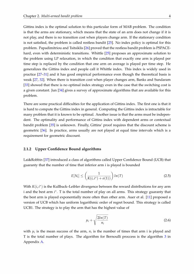
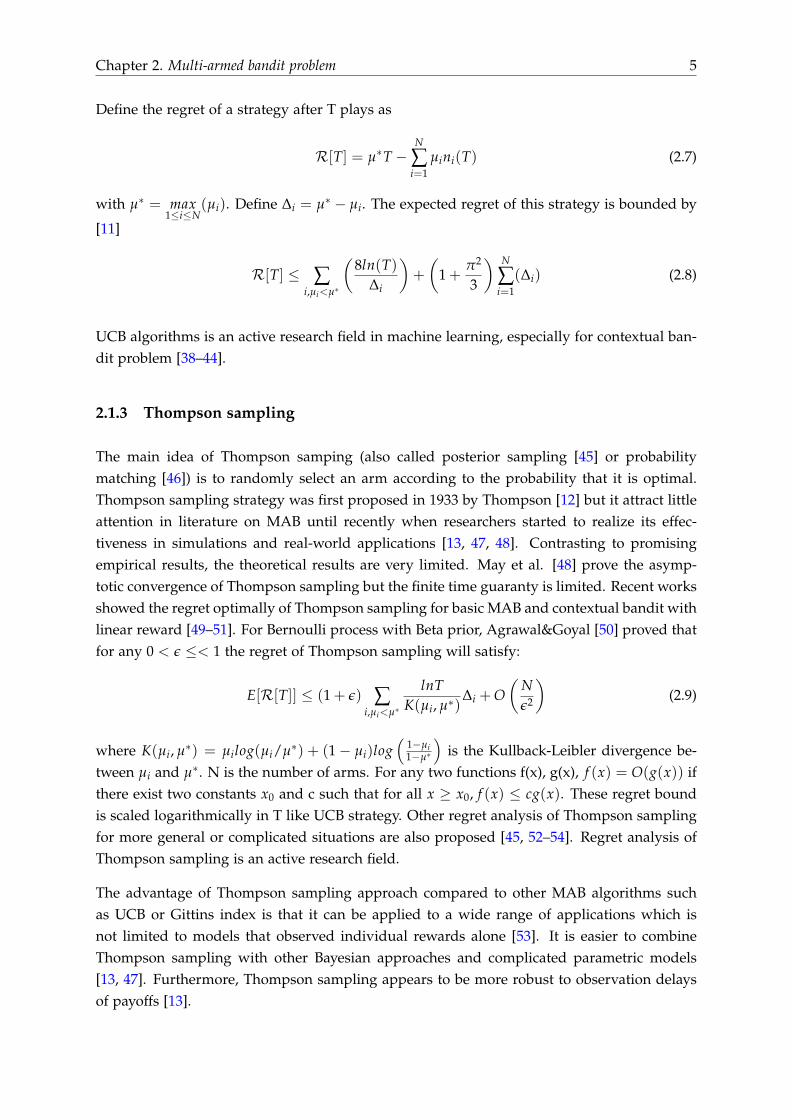
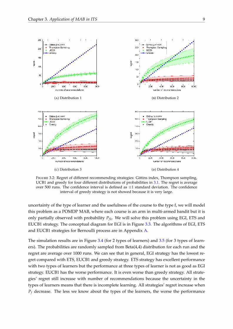
In figure 3.1, we plot the regret (2.7) of different MAB strategies. There are 10 courses thatthe ITS can recommends to learners and the probability of each course is randomly sampledfrom Beta(4,4) distribution for each run. The regret is averaged over 1000 runs. On the leftis the mean and confidence interval of the regret of different strategies. On the right is thedistribution of the regret at 10000th recommendation. The reason why we do not plot theconfidence interval of the regret of greedy strategy is that it is very large and the skewness islarge too (see the right hand side). In Figure 3.2, we plot the mean and confidence intervalfor four other distributions in 3.1. We can see that the Gittins index strategy give the bestresult but the Thompson sampling work as well as the Gittins index strategy. While the UCB1strategy guarantees that the regret is logarithmically bounded, its performance with finitenumber of learners is not good as good as other strategies. After 10000 recommendation,UCB1 strategy even performs worse than greedy strategy in distributions with large numberof courses. The standard deviation of regret of greedy strategy is very large because this strat-egy exploit too much. Greedy strategy sometimes gets stuck at courses with low probabilityof success (incomplete learning) and this cause the linear increase of regret. In contrast UCB1strategy has high regret because this strategy sends too much learners to inferior options forexploration which means that it explores too much. The choice of β for Gittins index strategyis depended on the number of recommend that the ITS will make. Suppose that ITS willmakes about 10000 recommendations and the discount is spread out evenly then the effectivediscount from one learner to the next is about 1/10000 suggesting β is about 0.9999. The valueof β is T

T+1 if the number of recommendation is T. 1− β can be understand as the probability

Chapter 3. Application of MAB in ITS 8

that the recommendation can stop. The distributions of probabilities we used are:

Distribution 1: 2 courses with p = 0.4, 0.6; (3.1)

Distribution 2: 4 courses with p = 0.3, 0.4, 0.5, 0.6;

Distribution 3: 10 courses with p = 0.30, 0.35, 0.40, 0.45, 0.50, 0.55, 0.60, 0.65, 0.70, 0.75;

Distribution 4: 10 courses with p = 0.30, 0.31, 0.32, 0.40, 0.41, 0.42, 0.50, 0.51, 0.52, 0.60

(a) Mean regret and confidence interval. (b) Distribution of the regret at 10000th recom-mendation.

Figure 3.1: The regret of different strategies: Gittins index, Thompson Sampling, UCB1 andgreedy. There are 10 courses that the ITS can recommends to learners and the probabilityof each course is randomly sampled from Beta(4,4) distribution for each run. The regretis averaged over 1000 runs. Left: mean regret and the confidence interval as a function ofnumber of recommendations. The confidence interval is defined as ±1 standard deviation.The confidence interval of greedy strategy is not showed because it is very large (look at theright figure). Right: distribution of the regret at 10000th recommendation. The star is the

mean, the circle is the 99 % and 1 % and the triangle is the maximum and minimum.

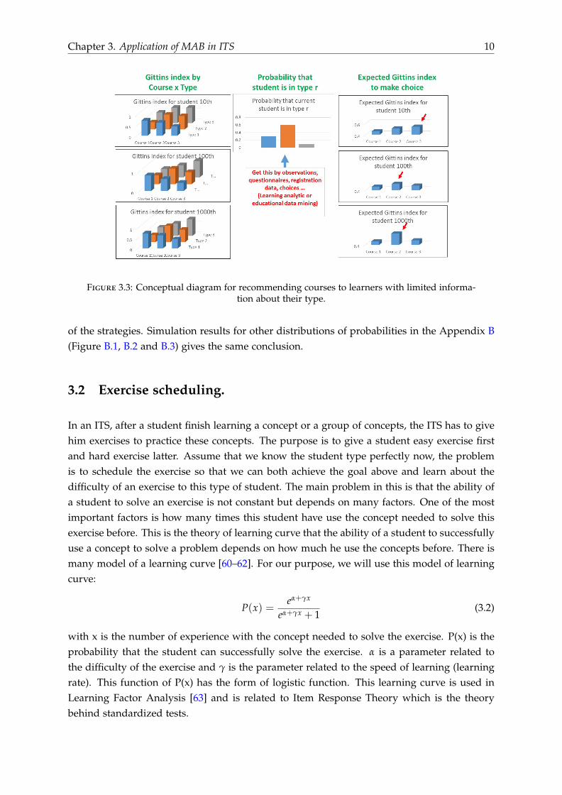
The problem with ITS is that learners are not homogeneous. In the learning context we haveto consider that learners will have various individual needs, preferences and characteristicssuch as different levels of expertise, knowledge, cognitive abilities, learning styles, motivation,preferences, and that they want to achieve a specific competence in a certain time. Thus, wecan’t not treat them in a uniform way. It is of great importance to provide a personalizedITS which can give adaptive recommendation taking into account the variety of learners’learning styles and knowledge levels. To do this, ITS often classified learners into groups ortypes based on characteristics of learners [2, 59]. Different types of learners will have differentprobability of success to a course. If we know exactly what are the types of learners, we canuse the data from learners of this type for calculating the Gittins index and recommend thebest course to them. If a learner stay long in the systems, we can identify well the type of thelearner. But the ITS has to give recommendation to learners when they are new and the ITScan only have a limited information about the learner. Assuming that student are classifiedinto F group and we know the type f of the learner k with probability Pf k. Given both the

Chapter 3. Application of MAB in ITS 9

(a) Distribution 1 (b) Distribution 2

(c) Distribution 3 (d) Distribution 4

Figure 3.2: Regret of different recommending strategies: Gittins index, Thompson sampling,UCB1 and greedy for four different distributions of probabilities in 3.1. The regret is averageover 500 runs. The confidence interval is defined as ±1 standard deviation. The confidence

interval of greedy strategy is not showed because it is very large.

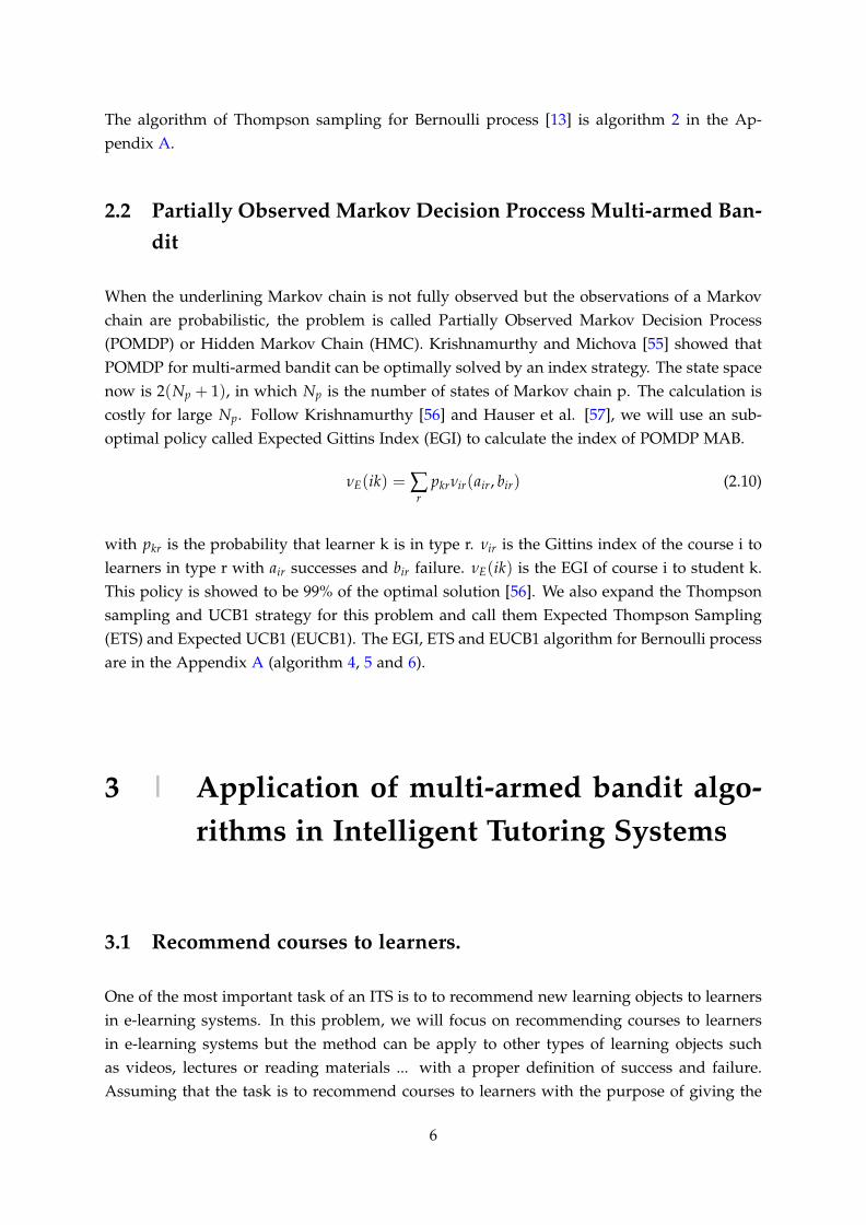
uncertainty of the type of learner and the usefulness of the course to the type f, we will modelthis problem as a POMDP MAB, where each course is an arm in multi-armed bandit but it isonly partially observed with probability Pf k. We will solve this problem using EGI, ETS andEUCB1 strategy. The conceptual diagram for EGI is in Figure 3.3. The algorithms of EGI, ETSand EUCB1 strategies for Bernoulli process are in Appendix A.

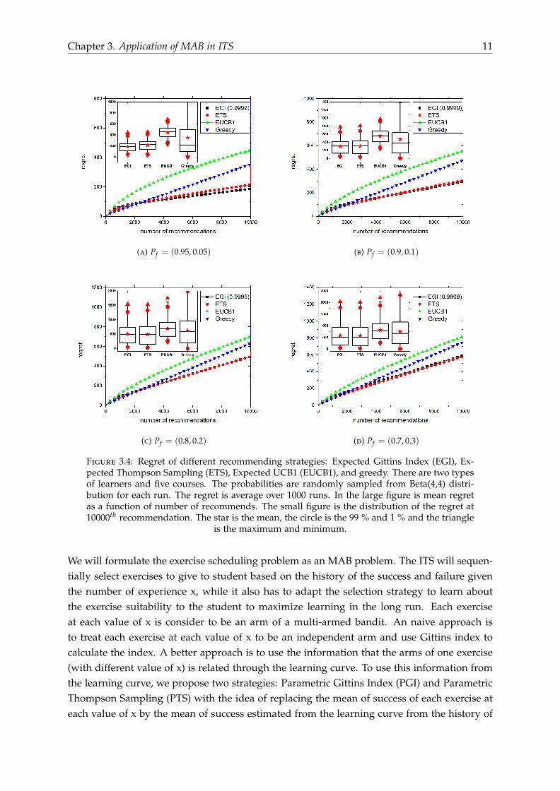
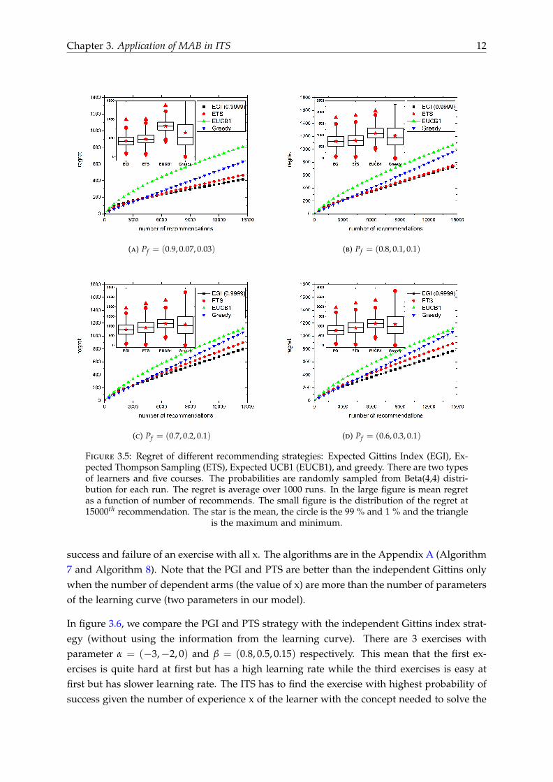
The simulation results are in Figure 3.4 (for 2 types of learners) and 3.5 (for 3 types of learn-ers). The probabilities are randomly sampled from Beta(4,4) distribution for each run and theregret are average over 1000 runs. We can see that in general, EGI strategy has the lowest re-gret compared with ETS, EUCB1 and greedy strategy. ETS strategy has excellent performancewith two types of learners but the performance at three types of learner is not as good as EGIstrategy. EUCB1 has the worse performance. It is even worse than greedy strategy. All strate-gies’ regret still increase with number of recommendations because the uncertainty in thetypes of learners means that there is incomplete learning. All strategies’ regret increase whenPf decrease. The less we know about the types of the learners, the worse the performance

Chapter 3. Application of MAB in ITS 10

Figure 3.3: Conceptual diagram for recommending courses to learners with limited informa-tion about their type.

of the strategies. Simulation results for other distributions of probabilities in the Appendix B(Figure B.1, B.2 and B.3) gives the same conclusion.

3.2 Exercise scheduling.

In an ITS, after a student finish learning a concept or a group of concepts, the ITS has to givehim exercises to practice these concepts. The purpose is to give a student easy exercise firstand hard exercise latter. Assume that we know the student type perfectly now, the problemis to schedule the exercise so that we can both achieve the goal above and learn about thedifficulty of an exercise to this type of student. The main problem in this is that the ability ofa student to solve an exercise is not constant but depends on many factors. One of the mostimportant factors is how many times this student have use the concept needed to solve thisexercise before. This is the theory of learning curve that the ability of a student to successfullyuse a concept to solve a problem depends on how much he use the concepts before. There ismany model of a learning curve [60–62]. For our purpose, we will use this model of learningcurve:

P(x) =eα+γx

eα+γx + 1(3.2)

with x is the number of experience with the concept needed to solve the exercise. P(x) is theprobability that the student can successfully solve the exercise. α is a parameter related tothe difficulty of the exercise and γ is the parameter related to the speed of learning (learningrate). This function of P(x) has the form of logistic function. This learning curve is used inLearning Factor Analysis [63] and is related to Item Response Theory which is the theorybehind standardized tests.

Chapter 3. Application of MAB in ITS 11

(a) Pf = (0.95, 0.05) (b) Pf = (0.9, 0.1)

(c) Pf = (0.8, 0.2) (d) Pf = (0.7, 0.3)

Figure 3.4: Regret of different recommending strategies: Expected Gittins Index (EGI), Ex-pected Thompson Sampling (ETS), Expected UCB1 (EUCB1), and greedy. There are two typesof learners and five courses. The probabilities are randomly sampled from Beta(4,4) distri-bution for each run. The regret is average over 1000 runs. In the large figure is mean regretas a function of number of recommends. The small figure is the distribution of the regret at10000th recommendation. The star is the mean, the circle is the 99 % and 1 % and the triangle

is the maximum and minimum.

We will formulate the exercise scheduling problem as an MAB problem. The ITS will sequen-tially select exercises to give to student based on the history of the success and failure giventhe number of experience x, while it also has to adapt the selection strategy to learn aboutthe exercise suitability to the student to maximize learning in the long run. Each exerciseat each value of x is consider to be an arm of a multi-armed bandit. An naive approach isto treat each exercise at each value of x to be an independent arm and use Gittins index tocalculate the index. A better approach is to use the information that the arms of one exercise(with different value of x) is related through the learning curve. To use this information fromthe learning curve, we propose two strategies: Parametric Gittins Index (PGI) and ParametricThompson Sampling (PTS) with the idea of replacing the mean of success of each exercise ateach value of x by the mean of success estimated from the learning curve from the history of

Chapter 3. Application of MAB in ITS 12

(a) Pf = (0.9, 0.07, 0.03) (b) Pf = (0.8, 0.1, 0.1)

(c) Pf = (0.7, 0.2, 0.1) (d) Pf = (0.6, 0.3, 0.1)

Figure 3.5: Regret of different recommending strategies: Expected Gittins Index (EGI), Ex-pected Thompson Sampling (ETS), Expected UCB1 (EUCB1), and greedy. There are two typesof learners and five courses. The probabilities are randomly sampled from Beta(4,4) distri-bution for each run. The regret is average over 1000 runs. In the large figure is mean regretas a function of number of recommends. The small figure is the distribution of the regret at15000th recommendation. The star is the mean, the circle is the 99 % and 1 % and the triangle

is the maximum and minimum.

success and failure of an exercise with all x. The algorithms are in the Appendix A (Algorithm7 and Algorithm 8). Note that the PGI and PTS are better than the independent Gittins onlywhen the number of dependent arms (the value of x) are more than the number of parametersof the learning curve (two parameters in our model).

In figure 3.6, we compare the PGI and PTS strategy with the independent Gittins index strat-egy (without using the information from the learning curve). There are 3 exercises withparameter α = (−3,−2, 0) and β = (0.8, 0.5, 0.15) respectively. This mean that the first ex-ercises is quite hard at first but has a high learning rate while the third exercises is easy atfirst but has slower learning rate. The ITS has to find the exercise with highest probability ofsuccess given the number of experience x of the learner with the concept needed to solve the

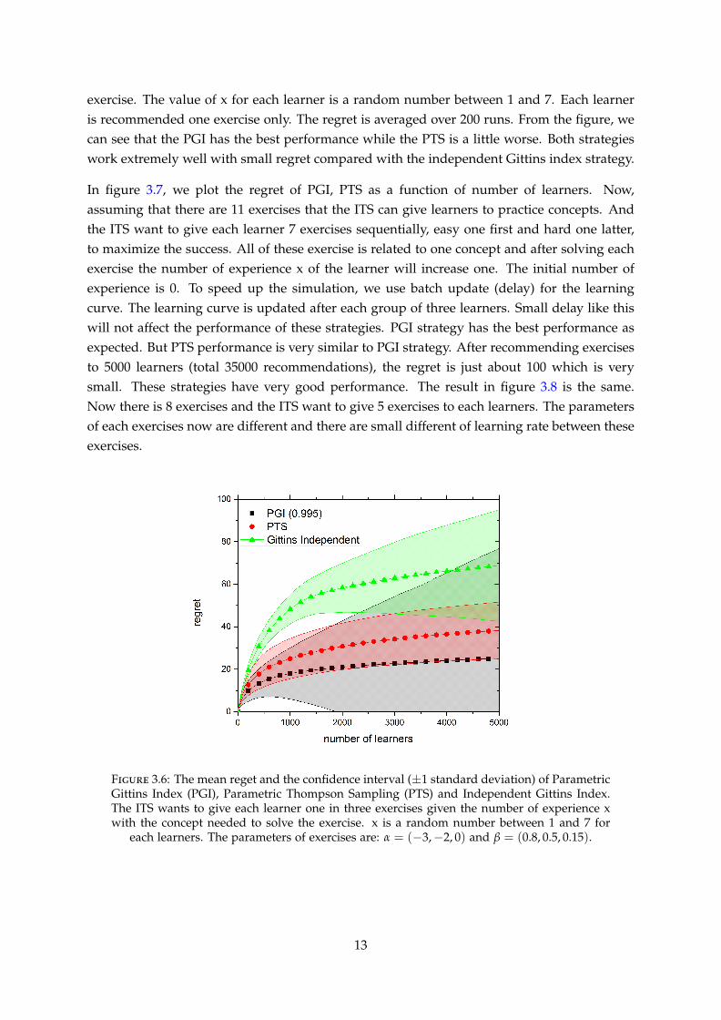
exercise. The value of x for each learner is a random number between 1 and 7. Each learneris recommended one exercise only. The regret is averaged over 200 runs. From the figure, wecan see that the PGI has the best performance while the PTS is a little worse. Both strategieswork extremely well with small regret compared with the independent Gittins index strategy.

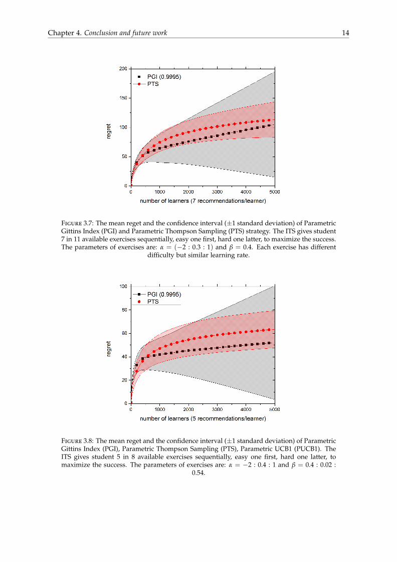
In figure 3.7, we plot the regret of PGI, PTS as a function of number of learners. Now,assuming that there are 11 exercises that the ITS can give learners to practice concepts. Andthe ITS want to give each learner 7 exercises sequentially, easy one first and hard one latter,to maximize the success. All of these exercise is related to one concept and after solving eachexercise the number of experience x of the learner will increase one. The initial number ofexperience is 0. To speed up the simulation, we use batch update (delay) for the learningcurve. The learning curve is updated after each group of three learners. Small delay like thiswill not affect the performance of these strategies. PGI strategy has the best performance asexpected. But PTS performance is very similar to PGI strategy. After recommending exercisesto 5000 learners (total 35000 recommendations), the regret is just about 100 which is verysmall. These strategies have very good performance. The result in figure 3.8 is the same.Now there is 8 exercises and the ITS want to give 5 exercises to each learners. The parametersof each exercises now are different and there are small different of learning rate between theseexercises.

Figure 3.6: The mean reget and the confidence interval (±1 standard deviation) of ParametricGittins Index (PGI), Parametric Thompson Sampling (PTS) and Independent Gittins Index.The ITS wants to give each learner one in three exercises given the number of experience xwith the concept needed to solve the exercise. x is a random number between 1 and 7 for

each learners. The parameters of exercises are: α = (−3,−2, 0) and β = (0.8, 0.5, 0.15).

13

Chapter 4. Conclusion and future work 14

Figure 3.7: The mean reget and the confidence interval (±1 standard deviation) of ParametricGittins Index (PGI) and Parametric Thompson Sampling (PTS) strategy. The ITS gives student7 in 11 available exercises sequentially, easy one first, hard one latter, to maximize the success.The parameters of exercises are: α = (−2 : 0.3 : 1) and β = 0.4. Each exercise has different

difficulty but similar learning rate.

Figure 3.8: The mean reget and the confidence interval (±1 standard deviation) of ParametricGittins Index (PGI), Parametric Thompson Sampling (PTS), Parametric UCB1 (PUCB1). TheITS gives student 5 in 8 available exercises sequentially, easy one first, hard one latter, tomaximize the success. The parameters of exercises are: α = −2 : 0.4 : 1 and β = 0.4 : 0.02 :

0.54.

Chapter 4. Conclusion and future work 15

4 | Conclusion and future work

In this project, we take an multi-armed bandit approach to ITS problems such as learningobjects recommendation and exercises scheduling. We propose methods and algorithms forthese problems based on MAB algorithms. We test the optimal strategies, Gittins index,together with Thompson sampling and Upper Confident Bound (UCB1) strategy. We alsopropose strategies to solve the learning objects recommendation with multiple types of learn-ers: Expected Gittins Index, Expected Thompson Sampling and Expected UCB1. For the taskof exercises scheduling, we modify the Gittins index strategy and the Thompson sampling toutilize the information from the learning curve and propose the Parametric Gittin Index andParametric Thompson Sampling. We still don’t know how to find the confidence bound forthe UCB1 strategy in this case. We test all of these strategy using simulation. Gittins index andGittins index based (EGI and PGI) strategies have the best performance but the Thompsonsampling and Thompson sampling based (ETS and PTS) have very good performance. WhileGittins index has one parameter β, Thompson sampling does not has any parameter. Thisis one advantage of Thompson sampling over Gittins index strategy. Furthermore, Thomp-son sampling has at the collective level the good property to be asymptotically convergentbecause all arm are tried an infinity number of time.

However, the stochastic feature of Thompson sampling can raise at the individual level someethical criticism: it is considering learners as "cobaye". Gittins index is taking into accountfor each learner the parameter β, that represent the compromise between exploration andexploitation for his/her own future. There is a deep relation for a given learner and a givenconcept between β and the mean number of times a concept will be used in his/her future (atleast until the final exam).

In the future, we want to investigate this multi-armed bandit approach to other tasks in ITSs.The recommending objects now are not only simple objects like courses or exercises but canbe a collection of learning objects such as a learning paths. The result now are not Bernoulliresult but we can use Gittins index, Thompson sampling or Upper Confidence Bound strategyfor normal processes. The grand task we want to tackle is designing a complete ITS withthere important part: a network of concepts for navigation, and a methods for classificationof learners and a recommending strategies for the balance between exploration vs exploitationin the systems. This project is the first step for this task.

At all level of an Intelligent Tutorial System, there are adaptive systems with their own com-promise between exploration and exploitation and with their own "life time horizon" thatare equivalent to some parameter β. Thus the multi-armed strategy and its approximationswill remain a must for future direction of research, especially in the context of MOOCs ineducation. Such big data context will allow more and more categorization for more accurateprediction at all level of each ITS.

Acknowledgements

I would like to express my gratitude to my supervisor - professor Paul Bourgine - for intro-ducing me to the topic as well for his support during the internship. Without his guidanceand persistent help this project would not have been possible. He has been a tremendousmentor for me. Furthermore, I would like to thank Nadine Peyriéras for providing me theinternship. I would also like to express my gratitude to Erasmus Mundus consortium fortheir support during my master.

16

A | Multi-armed bandit algorithms

A.1 Algorithms for independent Bernoulli Bandit

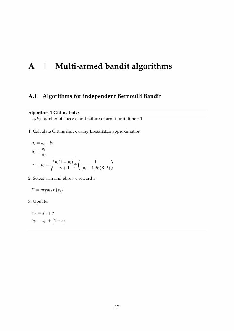
Algorithm 1 Gittins Indexai, bi: number of success and failure of arm i until time t-1

1. Calculate Gittins index using Brezzi&Lai approximation

ni = ai + bi

µi =ai

ni

νi = µi +

√µi(1− µi)

ni + 1ψ

(1

(ni + 1)ln(β−1)

)2. Select arm and observe reward r

i∗ = argmax {νi}

3. Update:

ai∗ = ai∗ + r

bi∗ = bi∗ + (1− r)

17

Appendix A. Algorithms 18

Algorithm 2 Thompson Samplingai, bi: number of success and failure of arm i until time t-1

1. Sample data from Beta distribution

φi ∼ Beta[ai, bi]

2. Select arm and observe reward r

i∗ = argmax {φi}

3. Update:

ai∗ = ai∗ + r

bi∗ = bi∗ + (1− r)

Algorithm 3 UCB1ai, bi: number of success and failure of arm i until time t-1

1. Find the index of each arm

νi =ai

ai + bi+

√2ln(t− 1)

ai + bi

1. Select arm and observe reward r

i∗ = argmax {νi}

3. Update:

ai∗ = ai∗ + r

bi∗ = bi∗ + (1− r)

Appendix A. Algorithms 19

A.2 Algorithms for POMDP Bernoulli Bandit

Algorithm 4 Expected Gittins IndexPf k: probability that player k are in group f. a f i, b f i: number of success and failure of arm i

of group f until time t-1.

1. Find the index of each arm i for each group f of learners.

n f i = a f i + b f i

µ f i =a f i

n f i

ν f i = µ f i +

√µ f i(1− µ f i)

n f i + 1ψ

(1

(n f i + 1)ln(β−1)

)2. Find the expected Gittins index of each course i to learner k

νEki = ∑

fPf kν f i

2. Select arm and observe reward r

i∗ = argmax{

νEki

}3. Update:

ai∗ f = ai∗ f + rPf k

bi∗ f = bi∗ f + (1− r)Pf k

Appendix A. Algorithms 20

Algorithm 5 Expected Thompson SamplingPf k: probability that player k are in group f. a f i, b f i: number of success and failure of arm i

of group f until time t-1.

1. Sample data for each arm i of each group f of learners.

φ f i ∼ Beta(a f i, b f i)

2. Find the expected Thompson sampling of each course i to learners k

φEki = ∑

fPf kφ f i

2. Select arm and observe reward r

i∗ = argmax{

φEki

}3. Update:

ai∗ f = ai∗ f + rPf k

bi∗ f = bi∗ f + (1− r)Pf k

Appendix A. Algorithms 21

Algorithm 6 Expected UCB1Pf k: probability that player k are in group f. a f i, b f i: number of success and failure of arm i

of group f until time t-1.

1. Find the index of each arm i for each group f of learners.

n f i = a f i + b f i

µ f i =a f i

n f i

ν f i = µ f i +

√√√√2ln(∑Nj=1 n f j)

n f i

2. Find the Expected UCB1 index of each course i to learner k

νEki = ∑

fPf kν f i

2. Select arm and observe reward r

i∗ = argmax{

νEki

}3. Update:

ai∗ f = ai∗ f + rPf k

bi∗ f = bi∗ f + (1− r)Pf k

Appendix A. Algorithms 22

A.3 Algorithms for Exercises Scheduling

Algorithm 7 Parametric Gittins Indexai(x), bi(x): number of success and failure of an exercise i with x is the number of experiencewith the concept needed to solve the exercise. xi is the number of experience with conceptneeded to solve the exercise i of current learner.Learning curve model: P(x) = eα+γx

eα+γx+1

1. Estimate the learning curve Pi(x) from ai(x), bi(x) using logistic regression.2. Find the index of each exercise i given xi

ni =∞

∑x=1

(ai(x) + bi(x))/2

µi = Pi(xi)

νi = µi +

√µi(1− µi)

ni + 1ψ

(1

(ni + 1)ln(β−1)

)2. Select arm and observe reward r

i∗ = argmax {νi}

3. Update:

ai∗(xi∗) = ai∗(xi∗) + r

bi∗(xi∗) = bi∗(xi∗) + (1− r)

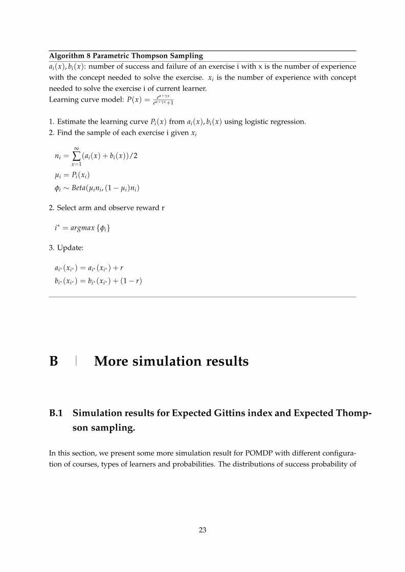
Algorithm 8 Parametric Thompson Samplingai(x), bi(x): number of success and failure of an exercise i with x is the number of experiencewith the concept needed to solve the exercise. xi is the number of experience with conceptneeded to solve the exercise i of current learner.Learning curve model: P(x) = eα+γx

eα+γx+1

1. Estimate the learning curve Pi(x) from ai(x), bi(x) using logistic regression.2. Find the sample of each exercise i given xi

ni =∞

∑x=1

(ai(x) + bi(x))/2

µi = Pi(xi)

φi ∼ Beta(µini, (1− µi)ni)

2. Select arm and observe reward r

i∗ = argmax {φi}

3. Update:

ai∗(xi∗) = ai∗(xi∗) + r

bi∗(xi∗) = bi∗(xi∗) + (1− r)

B | More simulation results

B.1 Simulation results for Expected Gittins index and Expected Thomp-son sampling.

In this section, we present some more simulation result for POMDP with different configura-tion of courses, types of learners and probabilities. The distributions of success probability of

23

Appendix B. More simulation results 24

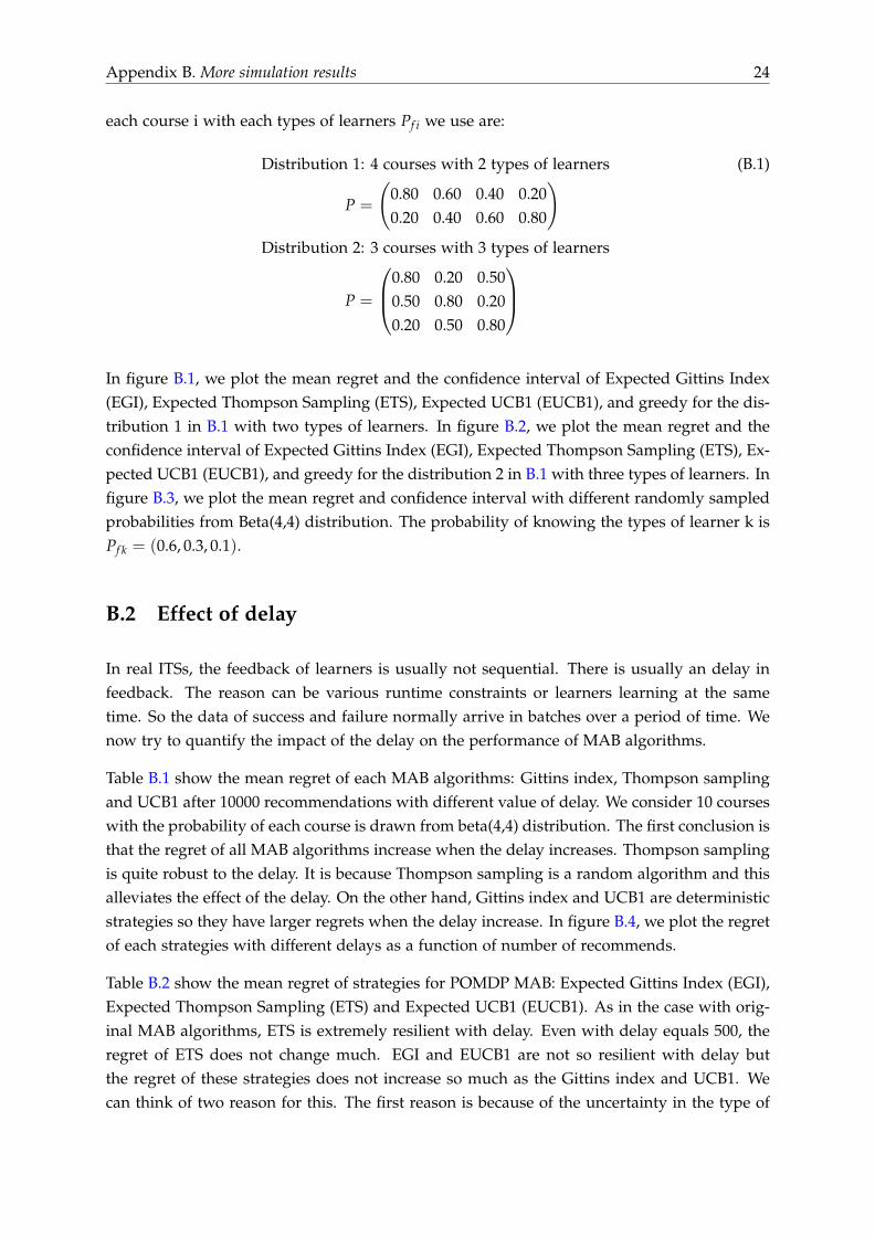
each course i with each types of learners Pf i we use are:

Distribution 1: 4 courses with 2 types of learners (B.1)

P =

(0.80 0.60 0.40 0.200.20 0.40 0.60 0.80

)Distribution 2: 3 courses with 3 types of learners

P =

0.80 0.20 0.500.50 0.80 0.200.20 0.50 0.80

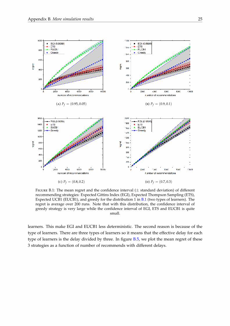
In figure B.1, we plot the mean regret and the confidence interval of Expected Gittins Index(EGI), Expected Thompson Sampling (ETS), Expected UCB1 (EUCB1), and greedy for the dis-tribution 1 in B.1 with two types of learners. In figure B.2, we plot the mean regret and theconfidence interval of Expected Gittins Index (EGI), Expected Thompson Sampling (ETS), Ex-pected UCB1 (EUCB1), and greedy for the distribution 2 in B.1 with three types of learners. Infigure B.3, we plot the mean regret and confidence interval with different randomly sampledprobabilities from Beta(4,4) distribution. The probability of knowing the types of learner k isPf k = (0.6, 0.3, 0.1).

B.2 Effect of delay

In real ITSs, the feedback of learners is usually not sequential. There is usually an delay infeedback. The reason can be various runtime constraints or learners learning at the sametime. So the data of success and failure normally arrive in batches over a period of time. Wenow try to quantify the impact of the delay on the performance of MAB algorithms.

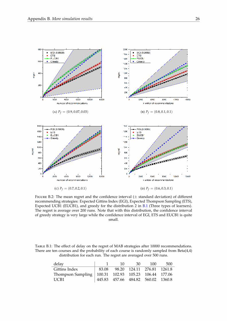
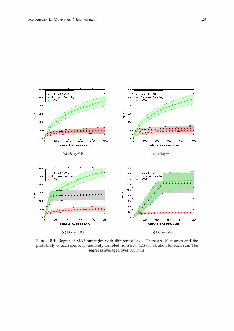
Table B.1 show the mean regret of each MAB algorithms: Gittins index, Thompson samplingand UCB1 after 10000 recommendations with different value of delay. We consider 10 courseswith the probability of each course is drawn from beta(4,4) distribution. The first conclusion isthat the regret of all MAB algorithms increase when the delay increases. Thompson samplingis quite robust to the delay. It is because Thompson sampling is a random algorithm and thisalleviates the effect of the delay. On the other hand, Gittins index and UCB1 are deterministicstrategies so they have larger regrets when the delay increase. In figure B.4, we plot the regretof each strategies with different delays as a function of number of recommends.

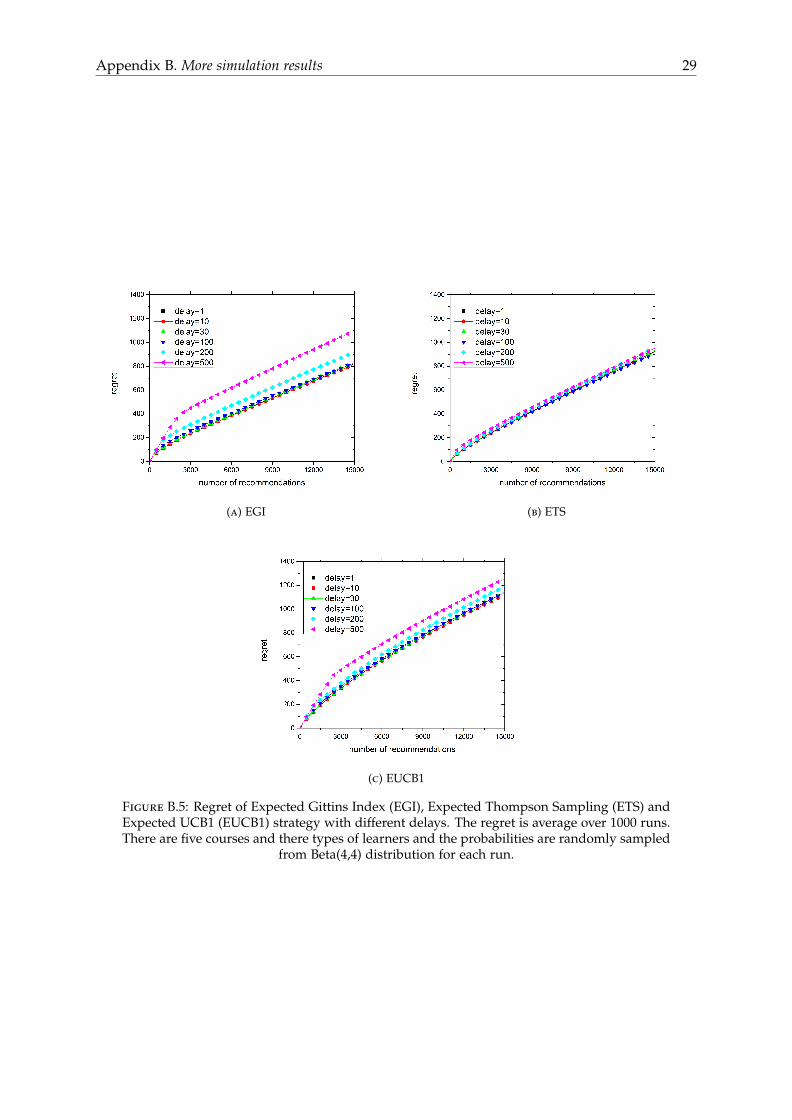
Table B.2 show the mean regret of strategies for POMDP MAB: Expected Gittins Index (EGI),Expected Thompson Sampling (ETS) and Expected UCB1 (EUCB1). As in the case with orig-inal MAB algorithms, ETS is extremely resilient with delay. Even with delay equals 500, theregret of ETS does not change much. EGI and EUCB1 are not so resilient with delay butthe regret of these strategies does not increase so much as the Gittins index and UCB1. Wecan think of two reason for this. The first reason is because of the uncertainty in the type of

Appendix B. More simulation results 25

(a) Pf = (0.95, 0.05) (b) Pf = (0.9, 0.1)

(c) Pf = (0.8, 0.2) (d) Pf = (0.7, 0.3)

Figure B.1: The mean regret and the confidence interval (± standard deviation) of differentrecommending strategies: Expected Gittins Index (EGI), Expected Thompson Sampling (ETS),Expected UCB1 (EUCB1), and greedy for the distribution 1 in B.1 (two types of learners). Theregret is average over 200 runs. Note that with this distribution, the confidence interval ofgreedy strategy is very large while the confidence interval of EGI, ETS and EUCB1 is quite

small.

learners. This make EGI and EUCB1 less deterministic. The second reason is because of thetype of learners. There are three types of learners so it means that the effective delay for eachtype of learners is the delay divided by three. In figure B.5, we plot the mean regret of these3 strategies as a function of number of recommends with different delays.

Appendix B. More simulation results 26

(a) Pf = (0.9, 0.07, 0.03) (b) Pf = (0.8, 0.1, 0.1)

(c) Pf = (0.7, 0.2, 0.1) (d) Pf = (0.6, 0.3, 0.1)

Figure B.2: The mean regret and the confidence interval (± standard deviation) of differentrecommending strategies: Expected Gittins Index (EGI), Expected Thompson Sampling (ETS),Expected UCB1 (EUCB1), and greedy for the distribution 2 in B.1 (Three types of learners).The regret is average over 200 runs. Note that with this distribution, the confidence intervalof greedy strategy is very large while the confidence interval of EGI, ETS and EUCB1 is quite

small.

Table B.1: The effect of delay on the regret of MAB strategies after 10000 recommendations.There are ten courses and the probability of each course is randomly sampled from Beta(4,4)

distribution for each run. The regret are averaged over 500 runs.

delay 1 10 30 100 500Gittins Index 83.08 98.20 124.11 276.81 1261.8Thompson Sampling 100.31 102.93 105.23 106.44 177.06UCB1 445.83 457.66 484.82 560.02 1360.8

Appendix B. More simulation results 27

(a) (b)

(c) (d)

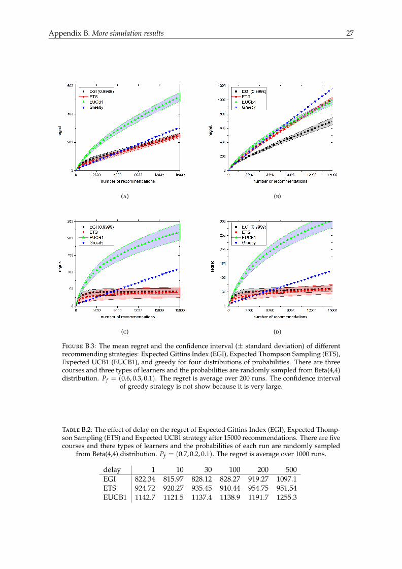
Figure B.3: The mean regret and the confidence interval (± standard deviation) of differentrecommending strategies: Expected Gittins Index (EGI), Expected Thompson Sampling (ETS),Expected UCB1 (EUCB1), and greedy for four distributions of probabilities. There are threecourses and three types of learners and the probabilities are randomly sampled from Beta(4,4)distribution. Pf = (0.6, 0.3, 0.1). The regret is average over 200 runs. The confidence interval

of greedy strategy is not show because it is very large.

Table B.2: The effect of delay on the regret of Expected Gittins Index (EGI), Expected Thomp-son Sampling (ETS) and Expected UCB1 strategy after 15000 recommendations. There are fivecourses and there types of learners and the probabilities of each run are randomly sampled

from Beta(4,4) distribution. Pf = (0.7, 0.2, 0.1). The regret is average over 1000 runs.

delay 1 10 30 100 200 500EGI 822.34 815.97 828.12 828.27 919.27 1097.1ETS 924.72 920.27 935.45 910.44 954.75 951,54EUCB1 1142.7 1121.5 1137.4 1138.9 1191.7 1255.3

Appendix B. More simulation results 28

(a) Delay=10 (b) Delay=30

(c) Delay=100 (d) Delay=500

Figure B.4: Regret of MAB strategies with different delays. There are 10 courses and theprobability of each course is randomly sampled from Beta(4,4) distribution for each run. The

regret is averaged over 500 runs.

Appendix B. More simulation results 29

(a) EGI (b) ETS

(c) EUCB1

Figure B.5: Regret of Expected Gittins Index (EGI), Expected Thompson Sampling (ETS) andExpected UCB1 (EUCB1) strategy with different delays. The regret is average over 1000 runs.There are five courses and there types of learners and the probabilities are randomly sampled

from Beta(4,4) distribution for each run.

Bibliography

[1] G. Adomavicius and A. Tuzhilin. Toward the next generation of recommender systems: a surveyof the state-of-the-art and possible extensions. IEEE Transactions on Knowledge and Data Engineering,17(6):734–749, June 2005. ISSN 1041-4347. URL http://ieeexplore.ieee.org/xpl/freeabs_all.jsp?arnumber=1423975.

[2] N Manouselis, H Drachsler, Katrien Verbert, and Erik Duval. Recommender systems for learning.2012. URL http://dspace.ou.nl/handle/1820/4647.

[3] Robin Burke. Hybrid recommender systems: Survey and experiments. User modeling and user-adapted interaction, 2002. URL http://link.springer.com/article/10.1023/A:1021240730564.

[4] Robin Burke. Hybrid web recommender systems. The adaptive web, pages 377–408, 2007. URLhttp://link.springer.com/chapter/10.1007/978-3-540-72079-9_12.

[5] LP Kaelbling, ML Littman, and AW Moore. Reinforcement Learning A Survey. arXiv preprintcs/9605103, 1996. URL http://arxiv.org/abs/cs/9605103.

[6] Dovev Lavie and Lori Rosenkopf. Balancing Exploration and Exploitation in Alliance Formation.Academy of Management Journal, 49(4):797–818, 2006. URL http://amj.aom.org/content/49/4/797.short.

[7] ND Daw, JP O’Doherty, Peter Dayan, Ben Seymour, and RJ Dolan. Cortical substrates for ex-ploratory decisions in humans. Nature, 441(7095):876–879, 2006. doi: 10.1038/nature04766.Cortical. URL http://www.nature.com/nature/journal/v441/n7095/abs/nature04766.html.

[8] Jonathan D Cohen, Samuel M McClure, and Angela J Yu. Should I stay or should I go?How the human brain manages the trade-off between exploitation and exploration. Philosoph-ical transactions of the Royal Society of London. Series B, Biological sciences, 362(1481):933–42, May2007. ISSN 0962-8436. doi: 10.1098/rstb.2007.2098. URL http://www.pubmedcentral.nih.gov/articlerender.fcgi?artid=2430007&tool=pmcentrez&rendertype=abstract.

[9] JC Gittins. Bandit processes and dynamic allocation indices. Journal of the Royal Statistical Society.Series B ( . . . , 41(2):148–177, 1979. URL http://www.jstor.org/stable/2985029.

[10] John Gittins, Kevin Glazebrook, and Richard Weber. Multi-armed Bandit Allocation Indices. Wiley,2011. ISBN 0470670029.

[11] Peter Auer, N Cesa-Bianchi, and P Fischer. Finite-time Analysis of the Multiarmed Bandit Prob-lem. Machine learning, pages 235–256, 2002. URL http://link.springer.com/article/10.1023/a:1013689704352.

30

Bibliography 31

[12] WR Thompson. On the Likelihood that One Unknown Probability Exceeds Another in View of theEvidence of Two Samples. Biometrika, 25(3):285–294, 1933. URL http://www.jstor.org/stable/2332286.

[13] Olivier Chapelle and L Li. An Empirical Evaluation of Thompson Sam-pling. NIPS, pages 1–9, 2011. URL https://papers.nips.cc/paper/4321-an-empirical-evaluation-of-thompson-sampling.pdf.

[14] Michael a. Talias. Optimal decision indices for R&D project evaluation in the pharmaceuticalindustry: Pearson index versus Gittins index. European Journal of Operational Research, 177(2):1105–1112, March 2007. ISSN 03772217. doi: 10.1016/j.ejor.2006.01.011. URL http://linkinghub.elsevier.com/retrieve/pii/S0377221706000385.

[15] Lihong Li, W Chu, John Langford, and X Wang. Unbiased offline evaluation of contextual-bandit-based news article recommendation algorithms. . . . conference on Web search and data . . . , 2011. URLhttp://dl.acm.org/citation.cfm?id=1935878.

[16] SC Watkinson, L Boddy, and K Burton. New approaches to investigating the function of mycelialnetworks. Mycologist, 2005. doi: 10.1017/S0269915XO5001023. URL http://www.sciencedirect.com/science/article/pii/S0269915X05001023.

[17] Stephen C Pratt and David J T Sumpter. A tunable algorithm for collective decision-making.Proceedings of the National Academy of Sciences of the United States of America, 103(43):15906–10,October 2006. ISSN 0027-8424. doi: 10.1073/pnas.0604801103. URL http://www.pubmedcentral.nih.gov/articlerender.fcgi?artid=1635101&tool=pmcentrez&rendertype=abstract.

[18] P Whittle. Multi-Armed Bandits and the Gittins Index. Journal of the Royal Statistical Society. SeriesB ( . . . , 42(2):143–149, 1980. URL http://www.jstor.org/stable/2984953.

[19] PP Varaiya. Extensions of the multiarmed bandit problem: the discounted case. AutomaticControl, IEEE . . . , (May):426–439, 1985. URL http://ieeexplore.ieee.org/xpls/abs_all.jsp?arnumber=1103989.

[20] R Weber. On the Gittins Index for Multiarmed Bandits. The Annals of Applied Probability, 2(4):1024–1033, 1992. URL http://projecteuclid.org/euclid.aoap/1177005588.

[21] Dimitris Bertsimas and J Niño Mora. Conservation Laws, Extended Polymatroids and MultiarmedBandit Problems; A Polyhedral Approach to Indexable Systems. Mathematics of Operations . . . , 21(2):257–306, 1996. URL http://pubsonline.informs.org/doi/abs/10.1287/moor.21.2.257.

[22] Jhelum Chakravorty and Aditya Mahajan. Multi-armed bandits, Gittins index, and its calculation.2013.

[23] Monica Brezzi and Tze Leung Lai. Optimal learning and experimentation in bandit prob-lems. Journal of Economic Dynamics and Control, 27(1):87–108, November 2002. ISSN 01651889.doi: 10.1016/S0165-1889(01)00028-8. URL http://linkinghub.elsevier.com/retrieve/pii/S0165188901000288.

[24] YC Yao. Some results on the Gittins index for a normal reward process. Time Series and RelatedTopics, 52:284–294, 2006. doi: 10.1214/074921706000001111. URL http://projecteuclid.org/euclid.lnms/1196285982.

Bibliography 32

[25] P Whittle. Restless bandits: Activity allocation in a changing world. Journal of applied probabil-ity, 25(May):287–298, 1988. URL http://scholar.google.com/scholar?hl=en&btnG=Search&q=intitle:Restless+Bandits:+Activity+Allocation+in+a+Changing+World#0.

[26] CH Papadimitriou and JN Tsitsiklis. The complexity of optimal queueing network control. Math-ematics of Operations . . . , 1999. URL http://pubsonline.informs.org/doi/abs/10.1287/moor.24.2.293.

[27] K.D. Glazebrook and H.M. Mitchell. An index policy for a stochastic scheduling model withimproving/deteriorating jobs. Naval Research Logistics, 49(7):706–721, October 2002. ISSN 0894-069X. doi: 10.1002/nav.10036. URL http://doi.wiley.com/10.1002/nav.10036.

[28] K.D. Glazebrook, H.M. Mitchell, and P.S. Ansell. Index policies for the maintenance of a collectionof machines by a set of repairmen. European Journal of Operational Research, 165(1):267–284, August2005. ISSN 03772217. doi: 10.1016/j.ejor.2004.01.036. URL http://linkinghub.elsevier.com/retrieve/pii/S0377221704000876.

[29] Jerome Le Ny, Munther Dahleh, and Eric Feron. Multi-UAV dynamic routing with partial obser-vations using restless bandit allocation indices. 2008 American Control Conference, pages 4220–4225,June 2008. doi: 10.1109/ACC.2008.4587156. URL http://ieeexplore.ieee.org/lpdocs/epic03/wrapper.htm?arnumber=4587156.

[30] Keqin Liu and Qing Zhao. Indexability of Restless Bandit Problems and Optimality of WhittleIndex for Dynamic Multichannel Access. IEEE Transactions on Information Theory, 56(11):5547–5567, November 2010. ISSN 0018-9448. doi: 10.1109/TIT.2010.2068950. URL http://ieeexplore.ieee.org/lpdocs/epic03/wrapper.htm?arnumber=5605371.

[31] Cem Tekin and Mingyan Liu. Online learning in opportunistic spectrum access: A restless banditapproach. INFOCOM, 2011 Proceedings IEEE, pages 2462–2470, April 2011. doi: 10.1109/INFCOM.2011.5935068. URL http://ieeexplore.ieee.org/xpls/abs_all.jsp?arnumber=5935068.

[32] RR Weber and G Weiss. On an Index Policy for Restless Bandits. Journal of Applied Probability, 27(3):637–648, 1990. URL http://www.jstor.org/stable/3214547.

[33] JS Banks and RK Sundaram. Switching costs and the Gittins index. Econometrica: Journal of theEconometric Society, 62(3):687–694, 1994. URL http://www.jstor.org/stable/2951664.

[34] Tackseung Jun. A survey on the bandit problem with switching costs. De Economist, 152(4):513–541, December 2004. ISSN 0013-063X. doi: 10.1007/s10645-004-2477-z. URL http://link.springer.com/10.1007/s10645-004-2477-z.

[35] John Langford and T Zhang. The epoch-greedy algorithm for contextual multi-armed bandits. Ad-vances in neural information processing . . . , pages 1–8, 2007. URL https://papers.nips.cc/paper/3178-the-epoch-greedy-algorithm-for-multi-armed-bandits-with-side-information.pdf.

[36] DA Berry and B Fristedt. Bandit Problems: Sequential Allocation of Experiments (Monographs onStatistics and Applied Probability). Springer, 1985. URL http://link.springer.com/content/pdf/10.1007/978-94-015-3711-7.pdf.

[37] TL Lai and H Robbins. Asymptotically efficient adaptive allocation rules. Advances in appliedmathematics, 22:4–22, 1985. URL http://scholar.google.com/scholar?hl=en&btnG=Search&q=intitle:Asymptotically+efficient+adaptive+allocation+rules#0.

Bibliography 33

[38] John N Tsitsiklis. Linearly parameterized bandits. Mathematics of Operations . . . , (1985):1–40, 2010.URL http://pubsonline.informs.org/doi/abs/10.1287/moor.1100.0446.

[39] Sarah Filippi, O Cappe, A Garivier, and C Szepesvári. Parametric Bandits: The Gen-eralized Linear Case. NIPS, pages 1–9, 2010. URL https://papers.nips.cc/paper/4166-parametric-bandits-the-generalized-linear-case.pdf.

[40] Miroslav Dudik, Daniel Hsu, and Satyen Kale. Efficient Optimal Learning for Contextual Bandits.arXiv preprint arXiv: . . . , 2011. URL http://arxiv.org/abs/1106.2369.

[41] S Bubeck and N Cesa-Bianchi. Regret analysis of stochastic and nonstochastic multi-armed banditproblems. arXiv preprint arXiv:1204.5721, 2012. URL http://arxiv.org/abs/1204.5721.

[42] Y Abbasi-Yadkori. Online-to-Confidence-Set Conversions and Application to Sparse Stochas-tic Bandits. Journal of Machine . . . , XX, 2012. URL http://david.palenica.com/papers/sparse-bandits/online-to-confidence-sets-conversion.pdf.

[43] Michal Valko, Alexandra Carpentier, and R Munos. Stochastic simultaneous optimistic opti-mization. Proceedings of the . . . , 28, 2013. URL http://machinelearning.wustl.edu/mlpapers/papers/valko13.

[44] Alekh Agarwal, Daniel Hsu, Satyen Kale, and John Langford. Taming the Monster: A Fastand Simple Algorithm for Contextual Bandits. arXiv preprint arXiv: . . . , pages 1–28, 2014. URLhttp://arxiv.org/abs/1402.0555.

[45] Daniel Russo and Benjamin Van Roy. Learning to Optimize Via Posterior Sampling. arXiv preprintarXiv:1301.2609, 00(0):1–29, 2013. doi: 10.1287/xxxx.0000.0000. URL http://arxiv.org/abs/1301.2609.

[46] SB Thrun. Efficient exploration in reinforcement learning. 1992. URL http://citeseerx.ist.psu.edu/viewdoc/summary?doi=10.1.1.45.2894.

[47] T Graepel. Web- Scale Bayesian Click-Through Rate Prediction for Sponsored Search Adver-tising in Microsofts Bing Search Engine. Proceedings of the . . . , 0(April 2009), 2010. URLhttp://machinelearning.wustl.edu/mlpapers/paper_files/icml2010_GraepelCBH10.pdf.

[48] BC May and DS Leslie. Simulation studies in optimistic Bayesian sampling in contextual-banditproblems. Statistics Group, Department of . . . , 01:1–29, 2011. URL http://nameless.maths.bris.ac.uk/research/stats/reports/2011/1102.pdf.

[49] Shipra Agrawal and N Goyal. Analysis of Thompson sampling for the multi-armed bandit prob-lem. arXiv preprint arXiv:1111.1797, 2011. URL http://arxiv.org/abs/1111.1797.

[50] Shipra Agrawal and N Goyal. Thompson sampling for contextual bandits with linear payoffs.arXiv preprint arXiv:1209.3352, 2012. URL http://arxiv.org/abs/1209.3352.

[51] Emilie Kaufmann, Nathaniel Korda, and R Munos. Thompson sampling: An asymptoticallyoptimal finite-time analysis. Algorithmic Learning Theory, pages 1–16, 2012. URL http://link.springer.com/chapter/10.1007/978-3-642-34106-9_18.

[52] S Bubeck and CY Liu. Prior-free and prior-dependent regret bounds for Thompson Sampling.Advances in Neural Information Processing . . . , pages 1–9, 2013. URL http://papers.nips.cc/paper/5108-prior-free-and-prior-dependent-regret-bounds-for-thompson-sampling.

Bibliography 34

[53] Aditya Gopalan, S Mannor, and Y Mansour. Thompson Sampling for Complex Online Problems.. . . of The 31st International Conference on . . . , 2014. URL http://jmlr.org/proceedings/papers/v32/gopalan14.html.

[54] Daniel Russo and Benjamin Van Roy. An Information-Theoretic Analysis of Thompson Sampling.arXiv preprint arXiv:1403.5341, pages 1–23, 2014. URL http://arxiv.org/abs/1403.5341.

[55] Vikram Krishnamurthy and Bo Wahlberg. Partially Observed Markov Decision Process Multi-armed Bandits—Structural Results. Mathematics of Operations Research, 34(2):287–302, May 2009.ISSN 0364-765X. doi: 10.1287/moor.1080.0371. URL http://pubsonline.informs.org/doi/abs/10.1287/moor.1080.0371.

[56] V. Krishnamurthy and J. Mickova. Finite dimensional algorithms for the hidden Markov modelmulti-armed bandit problem. 1999 IEEE International Conference on Acoustics, Speech, and SignalProcessing. Proceedings. ICASSP99 (Cat. No.99CH36258), pages 2865–2868 vol.5, 1999. doi: 10.1109/ICASSP.1999.761360. URL http://ieeexplore.ieee.org/lpdocs/epic03/wrapper.htm?arnumber=761360.

[57] JR Hauser and GL Urban. Website morphing. Marketing . . . , 2009. URL http://pubsonline.informs.org/doi/abs/10.1287/mksc.1080.0459.

[58] RF Kizilcec, Chris Piech, and E Schneider. Deconstructing disengagement: analyzing learnersubpopulations in massive open online courses. Proceedings of the third international . . . , 2013. URLhttp://dl.acm.org/citation.cfm?id=2460330.

[59] Aleksandra Klašnja-Milicevic, Boban Vesin, Mirjana Ivanovic, and Zoran Budimac. E-Learningpersonalization based on hybrid recommendation strategy and learning style identification. Com-puters & Education, 56(3):885–899, April 2011. ISSN 03601315. doi: 10.1016/j.compedu.2010.11.001.URL http://linkinghub.elsevier.com/retrieve/pii/S0360131510003222.

[60] LE Yelle. The learning curve: Historical review and comprehensive survey. Decision Sci-ences, 1979. URL http://onlinelibrary.wiley.com/doi/10.1111/j.1540-5915.1979.tb00026.x/abstract.

[61] PS Adler and KB Clark. Behind the learning curve: A sketch of the learning process. ManagementScience, 37(3):267–281, 1991. URL http://pubsonline.informs.org/doi/abs/10.1287/mnsc.37.3.267.

[62] FE Ritter and LJ Schooler. The learning curve. International encyclopedia of the social and . . . , pages1–12, 2001. URL http://acs.ist.psu.edu/papers/ritterS01.pdf.

[63] Hao Cen, Kenneth Koedinger, and Brian Junker. Learning factors analysis–a general methodfor cognitive model evaluation and improvement. Intelligent Tutoring Systems, 2006. URL http://link.springer.com/chapter/10.1007/11774303_17.