Embed Size (px)
Citation preview
13
Multi-armed Bandit with Additional Observations
DONGGYU YUN, Naver CorporationALEXANDRE PROUTIERE, KTHSUMYEONG AHN, JINWOO SHIN, and YUNG YI, KAIST
We study multi-armed bandit (MAB) problems with additional observations, where in each round, the decision
maker selects an arm to play and can also observe rewards of additional arms (within a given budget) by
paying certain costs. In the case of stochastic rewards, we develop a new algorithm KL-UCB-AO which is
asymptotically optimal when the time horizon grows large, by smartly identifying the optimal set of the
arms to be explored using the given budget of additional observations. In the case of adversarial rewards, we
propose H-INF, an algorithm with order-optimal regret. H-INF exploits a two-layered structure where in each
layer, we run a known optimal MAB algorithm. Such a hierarchical structure facilitates the regret analysis
of the algorithm, and in turn, yields order-optimal regret. We apply the framework of MAB with additional
observations to the design of rate adaptation schemes in 802.11-like wireless systems, and to that of online
advertisement systems. In both cases, we demonstrate that our algorithms leverage additional observations
to significantly improve the system performance. We believe the techniques developed in this paper are of
independent interest for other MAB problems, e.g., contextual or graph-structured MAB.
CCS Concepts: • Mathematics of computing → Probability and statistics; • Computing methodolo-gies →Machine learning; Sequential decision making;
ACM Reference Format:Donggyu Yun, Alexandre Proutiere, Sumyeong Ahn, Jinwoo Shin, and Yung Yi. 2018. Multi-armed Bandit
with Additional Observations. Proc. ACM Meas. Anal. Comput. Syst. 2, 1, Article 13 (March 2018), 22 pages.
https://doi.org/10.1145/3179416
1 INTRODUCTIONSince the seminal work by Robbins [30], the multi-armed bandit (MAB) problem (or simply bandit
problem) has received much attention due to a wide range of applications including medical trials,
online advertising [12, 34], recommendation systems [9], search engines [33] and wireless networks
[13]. In the classical MAB problem, the decision maker pulls in each round a single arm among
many arms, and observes the corresponding reward at the end of the round. The goal of the decisionmaker is to maximize the cumulative reward (over a fixed number of rounds), or equivalently to
minimize regret, defined as the difference between the cumulative reward and that achieved by
always playing the best arm. The expert problem is a variation of the classical MAB problem and
has also been extensively studied [4, 10, 11, 16, 19]: in this problem, at the end of round, the rewards
of all arms are revealed to the decision maker1. In the MAB literature, two popular models on
how rewards are generated have been considered: (a) stochastic – it assumes that rewards are i.i.d.
1Throughout this paper, the classicalMAB (or bandit) problem refers to the problem where only the reward of the played
arm is revealed.
Authors’ addresses: Donggyu Yun, [email protected], Naver Corporation; Alexandre Proutiere, [email protected], KTH;
Sumyeong Ahn, [email protected]; Jinwoo Shin, [email protected]; Yung Yi, [email protected], KAIST.
Permission to make digital or hard copies of all or part of this work for personal or classroom use is granted without fee
provided that copies are not made or distributed for profit or commercial advantage and that copies bear this notice and
the full citation on the first page. Copyrights for components of this work owned by others than ACM must be honored.
Abstracting with credit is permitted. To copy otherwise, or republish, to post on servers or to redistribute to lists, requires
prior specific permission and/or a fee. Request permissions from [email protected].
© 2018 Association for Computing Machinery.
2476-1249/2018/3-ART13 $$15.00
https://doi.org/10.1145/3179416
Proc. ACM Meas. Anal. Comput. Syst., Vol. 2, No. 1, Article 13. Publication date: March 2018.
13:2 Donggyu Yun et al.
across the various rounds and drawn from some unknown distributions, and (b) adversarial – it
allows an arbitrary (and adversarial) sequence of rewards.
This paper studies the MAB problem with additional observations. In each round, the decision
maker selects an arm to play, but also additional arms to observe the samples of their rewards.
Observing additional arms possibly incurs a cost, and also might be constrained by a given budget (in
terms of a maximum number of additional observations up to a given round). Similar versions of this
problem were first suggested by [32] and studied by [3, 20, 31], but only for the adversarial rewards.
They generalize both the classical MAB and expert problems: the former problem corresponds to
having no extra observations, whereas the latter corresponds to observing all arms in each round. In
this paper, we consider adversarial rewards, and provide, for the first time in this setting, algorithms
with tight regret upper bounds. We also consider stochastic rewards, and develop asymptotically
optimal algorithms. To our knowledge, MAB problems with additional observations with stochastic
rewards have not been investigated in the literature.
Additional observations come with a cost, which naturally arises in practical MAB applications
due to monetary or computational reasons. For example, in medical trials, a patient may consult
various doctors to get treatment advices which has to be paid. In wireless communication systems,
where packets have to be sent at different rates to probe the radio conditions of the channel, one
has to allocate some time for such a probing procedure [13]; this time cannot be used to transmit
actual data. For online advertisement in web services, one may wish to maintain ‘test’ websites,
simultaneously with ‘real’ ones, for additional feedback on advertisements, news articles, etc.
1.1 ContributionsFor stochastic rewards, we first derive an asymptotic lower bound on regret satisfied by any
algorithm. We then design KL-UCB-AO, an algorithm whose regret matches our lower bound. In
particular, when there exists no cost of additional observations, our results imply that a budget of
additional observations growing logarithmically with the time horizonT is necessary and sufficient
for obtaining a constant regret. The key idea of our algorithm is as follows. We first note that
similarly to [25], under any reasonable2algorithm, every suboptimal arm, say a, should be observed
at least fa(T ) = Ca logT times by roundT , for some well identified constantCa . Then, the idea is to
sort the arms in the ascending order of their expected rewards and use the observation budget for
each suboptimal arm a in that order to get fa(T ) observations, provided that the budget is enough
and observing arm a is more valuable than paying cost. Here the role of sorting is to play the arms
with larger expected rewards towards less regret.
For adversarial rewards, we restrict our attention to observation budgets growing linearly with
the time horizon, since sub-linear budgets can only have marginal impacts on regret in view of the
best known regret lower bound [31]. Due to this, unlike the case of stochastic rewards, we consider
no cost of additional observations: otherwise the regret should grow linearly. Note that we still have
a fixed budget for additional observations: a player can observe the rewards of a constant number
M of arms in each round for some M ≥ 1 and there is no extra cost for observing the additional
arms. This problem is a special case of known settings in the literature [3, 20, 31]. For this problem,
we design H-INF, an algorithm with regretO
(max
√NMT ,
√T logN
)for N arms,M observations,
andT rounds. The regret of H-INF improves those of the known algorithms [3, 20, 31] and matches
the lower bound derived in [31]. The design of H-INF is based on a novel two-layered structure,
where each layer runs the optimal INF algorithm [4]. In H-INF, one can replace the INF algorithm
by any other algorithm, as long as it is order-optimal for both the classical MAB (i.e.,M = 1) and
2i.e., uniformly good.
Proc. ACM Meas. Anal. Comput. Syst., Vol. 2, No. 1, Article 13. Publication date: March 2018.
Multi-armed Bandit with Additional Observations 13:3
the expert problem (i.e., M = N ). This simple, yet powerful hierarchical structure, allows us to
decouple the algorithmic components into layers, which significantly facilitates the regret analysis.
1.2 Related WorkWe first review the literature for the classical settings of MAB and expert problems. For the classical
MAB problem under stochastic rewards, Lai and Robbins [25] derived an asymptotic regret lower
bound satisfied by any algorithm. They also designed an algorithm based on the so-called upperconfidence bound (UCB), whose variants including UCB1 [5], Bayes-UCB [21] and KL-UCB [17] have
been proposed to improve the regret upper bound. Note that the optimal algorithm for the expert
problem (i.e.,M = N ) under stochastic rewards is somewhat trivial, i.e., following the decision of
the best arm in its empirical mean. For the classical MAB problem under adversarial rewards, the
EXP3 algorithm achieves the regret O(√
TN logN)[6], and the order-optimal regret O
(√TN
)is
achieved by the INF algorithm [4]. The well-known regret lower bound for the expert problem
under adversarial rewards isO(√
T logN), which can be achieved by several algorithms [4, 11, 16].
The additional observations or experts (i.e., 1 ≤ M ≤ N ) studied in this paper generalizes the
above classical settings. A version of this problem for the adversarial rewards was first suggested by
[32] as an open question and resolved by [20]. The proposed algorithm in [20] have regretO(√TN
)in our setting and it is clearly sub-optimal as it does not even depend on M .
3This is primarily
because the author studies a more general assumption on experts than ours: each expert provides a
probability distribution over all arms for selecting which arm to play, whereas we force every expert
i to play the arm i . Similar problems with the same assumption on experts as ours were also studied
[3, 31], where both algorithms have regret O
(√NMT logN
)in our setting, which is sub-optimal
by a logarithmic factor O(√
logN)for 1 ≤ M ≤ N /logN . They consider more general budget
constraints than ours for additional observations: time-varying budget [31] and cost-related budget
[3], which makes our H-INF algorithm not directly applicable to their settings. We again emphasize
that the above prior work only considered the adversarial rewards. For stochastic rewards, we
are unaware of any attempt to design asymptotically optimal algorithms considering additional
observations. Table 1 summarizes the related work as well as our contributions. In summary,
we study a special version of problems studied in [3, 20, 31] for the adversarial rewards, and its
stochastic version is first studied in this paper. For both types of rewards, we provide the first
optimal regret upper bounds.
We also remark that the MAB problem with graph-structured feedbacks [2, 8, 9, 23, 26] has asimilar flavor to our problem. However, the difference is that observations in prior work are given
by an external graph (i.e., playing an arm reveals the rewards of all neighboring arms under the
graph), while we can choose them adaptively over time without graphical restrictions, but with
cost and/or budget constraints. Nevertheless, we believe that the design principle of our algorithm
might also apply to the MAB problems with graph-structured feedback as well as other related
ones [3, 20, 31]. As other related work, paying for exploration is also studied in the principal-agent
framework [15, 27]. The authors assume that there is a principal or an organizer facing a MAB
problem, which, however, does not pull an arm directly: a myopic agent who arrives at each round
plays an arm instead of the principal. Since each myopic agent typically selects the arm with the
3The regret upper bound of [20] is 4
√minK,M N log
8MminK,M
M T for K arms and N experts. In our setting, K = N , hence it
becomes O(√T N
).
Proc. ACM Meas. Anal. Comput. Syst., Vol. 2, No. 1, Article 13. Publication date: March 2018.
13:4 Donggyu Yun et al.
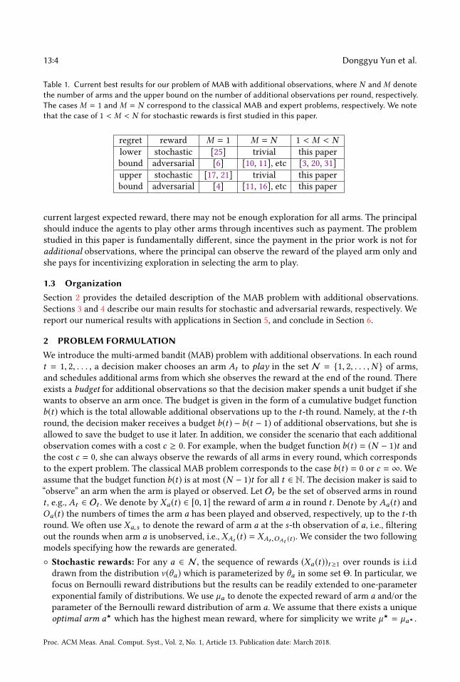
Table 1. Current best results for our problem of MAB with additional observations, where N andM denotethe number of arms and the upper bound on the number of additional observations per round, respectively.The cases M = 1 and M = N correspond to the classical MAB and expert problems, respectively. We notethat the case of 1 < M < N for stochastic rewards is first studied in this paper.
regret reward M = 1 M = N 1 < M < Nlower stochastic [25] trivial this paper
bound adversarial [6] [10, 11], etc [3, 20, 31]
upper stochastic [17, 21] trivial this paper
bound adversarial [4] [11, 16], etc this paper
current largest expected reward, there may not be enough exploration for all arms. The principal
should induce the agents to play other arms through incentives such as payment. The problem
studied in this paper is fundamentally different, since the payment in the prior work is not for
additional observations, where the principal can observe the reward of the played arm only and
she pays for incentivizing exploration in selecting the arm to play.
1.3 OrganizationSection 2 provides the detailed description of the MAB problem with additional observations.
Sections 3 and 4 describe our main results for stochastic and adversarial rewards, respectively. We
report our numerical results with applications in Section 5, and conclude in Section 6.
2 PROBLEM FORMULATIONWe introduce the multi-armed bandit (MAB) problem with additional observations. In each round
t = 1, 2, . . . , a decision maker chooses an arm At to play in the set N = 1, 2, . . . ,N of arms,
and schedules additional arms from which she observes the reward at the end of the round. There
exists a budget for additional observations so that the decision maker spends a unit budget if she
wants to observe an arm once. The budget is given in the form of a cumulative budget function
b(t) which is the total allowable additional observations up to the t-th round. Namely, at the t-thround, the decision maker receives a budget b(t) − b(t − 1) of additional observations, but she is
allowed to save the budget to use it later. In addition, we consider the scenario that each additional
observation comes with a cost c ≥ 0. For example, when the budget function b(t) = (N − 1)t andthe cost c = 0, she can always observe the rewards of all arms in every round, which corresponds
to the expert problem. The classical MAB problem corresponds to the case b(t) = 0 or c = ∞. We
assume that the budget function b(t) is at most (N − 1)t for all t ∈ N. The decision maker is said to
“observe” an arm when the arm is played or observed. Let Ot be the set of observed arms in round
t , e.g., At ∈ Ot . We denote by Xa(t) ∈ [0, 1] the reward of arm a in round t . Denote by Aa(t) andOa(t) the numbers of times the arm a has been played and observed, respectively, up to the t-thround. We often use Xa,s to denote the reward of arm a at the s-th observation of a, i.e., filteringout the rounds when arm a is unobserved, i.e., XAt (t) = XAt ,OAt (t ). We consider the two following
models specifying how the rewards are generated.
Stochastic rewards: For any a ∈ N , the sequence of rewards (Xa(t))t ≥1 over rounds is i.i.ddrawn from the distribution ν (θa) which is parameterized by θa in some set Θ. In particular, we
focus on Bernoulli reward distributions but the results can be readily extended to one-parameter
exponential family of distributions. We use µa to denote the expected reward of arm a and/or the
parameter of the Bernoulli reward distribution of arm a. We assume that there exists a unique
optimal arm a⋆ which has the highest mean reward, where for simplicity we write µ⋆ = µa⋆ .
Proc. ACM Meas. Anal. Comput. Syst., Vol. 2, No. 1, Article 13. Publication date: March 2018.
Multi-armed Bandit with Additional Observations 13:5
Without loss of generality, we order arms with respect to their expected rewards, i.e., a⋆ = Nand µ1 ≤ · · · < µN = µ⋆. Let Ω be the set µ ∈ (0, 1)N : µ1 ≤ µ2 ≤ . . . < µN .
Adversarial rewards: A non-oblivious adversary arbitrarily chooses rewards of arms, where she
may take into account the player’s past decisions on assigning rewards. The adversary has only
to decide the sequence of rewards (Xa(t) : a ∈ N) before the decision maker selects the observed
arms Ot in each t-th round. It is the most general scenario in the adversarial reward setting.
In each round, a decision rule or algorithm selects an arm to play and additional arms to observe,
depending on the arms observed in earlier rounds, their observed rewards and the budget function
b(t). The goal is to minimize the (expected) regret up to the round T , defined as:
R(T ) = max
a∈NE
[T∑t=1
Xa(t)
]− E
[T∑t=1
XAt (t) − c (|Ot | − 1)
]where the expectation E is taken over the possibly random rewards and the possible randomness
in the selected arms. Note that in the stochastic setting, the regret can be written as:
R(T ) = µ⋆T −∑a∈N
µaE [Aa(T )] + c∑a∈N
E [Oa(T ) −Aa(T )]
=∑a,a⋆
∆aE [Aa(T )] + c∑a∈N
E [Oa(T ) −Aa(T )] ,
where ∆a = µ⋆ − µa .
3 STOCHASTIC REWARDSIn this section, we study the MAB problem with additional observations in the stochastic setting.
For the classical MAB problem, it is known that any algorithm has Ω(log(T )) regret [25]. Onecan expect that additional observations would naturally reduce the regret. Given budget function
b(t) on additional observations up to the t-th round, we first derive an asymptotic lower bound
on the regret satisfied by any algorithm. Then, we devise KL-UCB-AO (KL-UCB with Additional
Observations), an algorithm whose regret matches the lower bound.
3.1 Regret Lower BoundRecall that we assume that arms are ordered with respect to their expected rewards, i.e., a⋆ = N .
Given the budget b(t) and the parameters µ = (µ1, . . . , µN ) ∈ Ω, we define a† , a⋆ as the arm with
minimum index such that
a†∑i=1
1
KL(µi ∥ µN )≥ lim
T→∞
b(T )
logT,
whereKL(p ∥ q) := p log(pq )+ (1−p) log(
1−p1−q ) denotes the Kullback-Leibler (KL) divergence between
two Bernoulli distributions with means p and q. If there is no such arm, we set a† = a⋆. We also
define the arm a‡ by a‡ := mini ∈ 1, . . . ,N − 1 | ∆i ≤ c. Similar to a†, if there is no such arm,
we let a‡ = a⋆.We say that an algorithm is uniformly good if its regret satisfies R(T ) = o(T α ) for all α > 0
regardless of µ ∈ Ω. The following theorem states an asymptotic lower bound on regret satisfied
by any uniformly good algorithm. Note that uniformly good algorithms exist, e.g., KL-UCB without
spending any observation budget is uniformly good.
Proc. ACM Meas. Anal. Comput. Syst., Vol. 2, No. 1, Article 13. Publication date: March 2018.
13:6 Donggyu Yun et al.
Theorem 3.1. For all µ = (µ1, . . . µN ) ∈ Ω, any uniformly good algorithm satisfies:if a† < a‡,
lim inf
T→∞
R(T )
logT≥
N−1∑i=a†+1
∆i
KL(µi ∥ µN )+ c lim
T→∞
b(T )
logT+ ∆a†
©«a†∑i=1
1
KL(µi ∥ µN )− lim
T→∞
b(T )
logT
ª®¬ .otherwise,
lim inf
T→∞
R(T )
logT≥
N−1∑i=a‡
∆i
KL(µi ∥ µN )+
a‡−1∑i=1
c
KL(µi ∥ µN )
The proof of Theorem 3.1 is given in Section 3.3. It is based on the following observations: (i) inorder to minimize the regret, we should not make additional observations for arms i having smaller
∆i than c , (ii) since playing an arm with a smaller expected reward incurs larger regret, we should
use the additional budget to observe such arms. These immediately induce a virtual policy and no
algorithm can have a better regret than this. Here, the two arms a† and a‡ become the thresholdarms. The observations of arms having lower expected reward than a† are done by only using the
budget. On the contrary, the observations of arms having higher expected reward than a‡ and a‡
are done by only playing these arms, i.e., the budget is never used for arms a‡, . . . ,N
Whenb(t) = 0, i.e., no additional observation, the regret lower bound in Theorem 3.1 matches that
of the classical MAB problem [25]. Moreover, Theorem 3.1 implies that a small budget b(t) = o(log t)does not have any effect on the asymptotic regret lower bound. However, when the budget is
enough so that limT→∞b(T )logT >
∑N−1i=1
1
KL(µi ∥ µN ), and we can use the budget with no cost (i.e., c = 0),
the regret might be sub-logarithmic with respect to the number of rounds, i.e., R(T )/logT → 0.
This is confirmed by the algorithm we propose in the following section.
3.2 KL-UCB-AO AlgorithmInspired by the regret lower bound derived in the previous section, we design the following
algorithm, called KL-UCB-AO, which is based on KL-UCB [17] designed for the classical MAB
problem.
The following theorem states the asymptotic optimality of KL-UCB-AO.
Theorem 3.2. For all µ = (µ1, . . . µN ) ∈ (0, 1)N , the regret of KL-UCB-AO satisfies:
i) if a† < a‡, then
lim sup
T→∞
R(T )
logT≤
N−1∑i=a†+1
∆i
KL(µi ∥ µN )+ c lim
T→∞
b(T )
logT+ ∆a†
©«a†∑i=1
1
KL(µi ∥ µN )− lim
T→∞
b(T )
logT
ª®¬ .ii) if a† ≥ a‡, a‡ , N or c , 0, a† = a‡ = N , then
lim sup
T→∞
R(T )
logT≤
N−1∑i=a‡
∆i
KL(µi ∥ µN )+
a‡−1∑i=1
c
KL(µi ∥ µN ).
iii) otherwise (i.e., c = 0, a† = a‡ = N ),
lim sup
T→∞
R(T ) < ∞.
Proc. ACM Meas. Anal. Comput. Syst., Vol. 2, No. 1, Article 13. Publication date: March 2018.
Multi-armed Bandit with Additional Observations 13:7
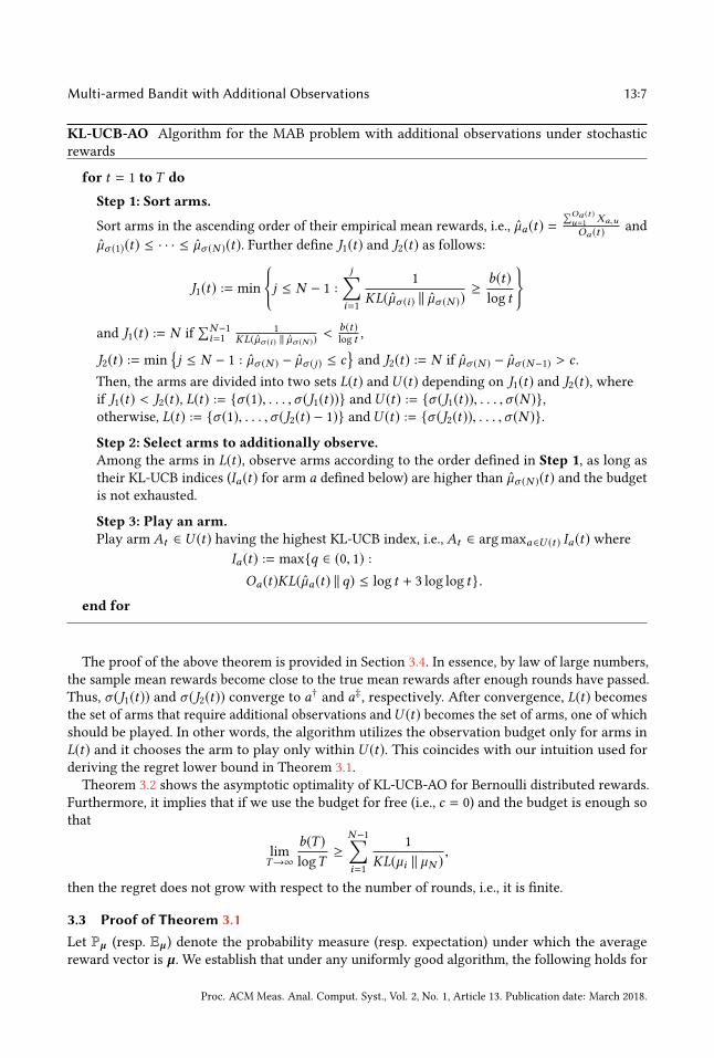
KL-UCB-AO Algorithm for the MAB problem with additional observations under stochastic
rewards
for t = 1 to T do
Step 1: Sort arms.
Sort arms in the ascending order of their empirical mean rewards, i.e., µa(t) =∑Oa (t )u=1 Xa,uOa (t )
and
µσ (1)(t) ≤ · · · ≤ µσ (N )(t). Further define J1(t) and J2(t) as follows:
J1(t) := min
j ≤ N − 1 :
j∑i=1
1
KL(µσ (i) ∥ µσ (N ))≥
b(t)
log t
and J1(t) := N if
∑N−1i=1
1
KL(µσ (i ) ∥ µσ (N ))< b(t )
log t ,
J2(t) := min
j ≤ N − 1 : µσ (N ) − µσ (j) ≤ c
and J2(t) := N if µσ (N ) − µσ (N−1) > c .
Then, the arms are divided into two sets L(t) andU (t) depending on J1(t) and J2(t), whereif J1(t) < J2(t), L(t) := σ (1), . . . ,σ (J1(t)) andU (t) := σ (J1(t)), . . . ,σ (N ),
otherwise, L(t) := σ (1), . . . ,σ (J2(t) − 1) andU (t) := σ (J2(t)), . . . ,σ (N ).
Step 2: Select arms to additionally observe.Among the arms in L(t), observe arms according to the order defined in Step 1, as long as
their KL-UCB indices (Ia(t) for arm a defined below) are higher than µσ (N )(t) and the budget
is not exhausted.
Step 3: Play an arm.Play arm At ∈ U (t) having the highest KL-UCB index, i.e., At ∈ argmaxa∈U (t ) Ia(t) where
Ia(t) := maxq ∈ (0, 1) :
Oa(t)KL(µa(t) ∥ q) ≤ log t + 3 log log t.
end for
The proof of the above theorem is provided in Section 3.4. In essence, by law of large numbers,
the sample mean rewards become close to the true mean rewards after enough rounds have passed.
Thus, σ (J1(t)) and σ (J2(t)) converge to a†and a‡, respectively. After convergence, L(t) becomes
the set of arms that require additional observations andU (t) becomes the set of arms, one of which
should be played. In other words, the algorithm utilizes the observation budget only for arms in
L(t) and it chooses the arm to play only within U (t). This coincides with our intuition used for
deriving the regret lower bound in Theorem 3.1.
Theorem 3.2 shows the asymptotic optimality of KL-UCB-AO for Bernoulli distributed rewards.
Furthermore, it implies that if we use the budget for free (i.e., c = 0) and the budget is enough so
that
lim
T→∞
b(T )
logT≥
N−1∑i=1
1
KL(µi ∥ µN ),
then the regret does not grow with respect to the number of rounds, i.e., it is finite.
3.3 Proof of Theorem 3.1Let Pµ (resp. Eµ ) denote the probability measure (resp. expectation) under which the average
reward vector is µ. We establish that under any uniformly good algorithm, the following holds for
Proc. ACM Meas. Anal. Comput. Syst., Vol. 2, No. 1, Article 13. Publication date: March 2018.
13:8 Donggyu Yun et al.
any µ ∈ Ω and any suboptimal arm a , N ,
lim inf
T→∞
Eµ[Oa(T )]
logT≥
1
KL(µa ∥ µN ). (1)
This inequality can be proved as in the classical bandit literature [25] using a so-called change-
of-measure argument. Recently the authors of [22] simplified this argument (see Theorem 21 and
its proof), and we can directly use it to show (1). More precisely, for a suboptimal arm a , N ,
consider a new reward vector µ = (µ1, . . . , µa−1, µ, µa+1, . . . , µN ) in which only µa is replaced
by µ, where µN < µ < 1. Hence, the arm a becomes the unique optimal arm under µ. We can
then show, using the same reasoning as in [22] (refer to the appendix for a detailed proof), that
lim infT→∞E[Oa (T )]logT ≥ 1
KL(µa ∥ µ) . Since we can take arbitrarily µN < µ < 1 and KL(µa ∥ µ) is
continuous w.r.t. µ, (1) can be derived. Note that several uniformly good algorithms (e.g., KL-UCB)
show the tightness of the inequality (1) (see Theorem 1 in [17]), which readily implies that every
suboptimal arm a should be observed asymptotically logT /KL(µa ∥ µN ) times by round T to have
R(T ) = o(T α ) for any α > 0.
Now, we just minimize the regret subject to the above constraints. To do so, notice the following:
(i) the regret increment by playing an arm in a‡, . . . ,N − 1 is less than or equal to c , (ii) playingan arm with smaller µ incurs a larger regret. From (i) and (ii), the solution is as follows: Sort the
arms in the ascending order of the expected rewards and spend the observation budget on each
arm a ∈ 1, . . . ,a‡ − 1 in that order just as much as (asymptotically) logT /KL(µa ∥ µN ) until thebudget is exhausted (in that case, the budget becomes empty in arm a†’s turn). Then, we have
if a† < a‡,
lim inf
T→∞
E[Aa(T )]
logT≥
0 if a ∈ 1, . . . ,a† − 1,a†∑i=1
1
KL(µa ∥ µN )− lim
T→∞
b(T )
logTif a = a†,
1
KL(µa ∥ µN )if a ∈ a† + 1, . . . ,N − 1,
and
lim inf
T→∞
E[Oa(T ) −Aa(T )]
logT≥
1
KL(µa ∥ µN )if a ∈ 1, . . . ,a† − 1,
lim
T→∞
b(T )
logT−
a†−1∑i=1
1
KL(µa ∥ µN )if a = a†,
0 if a ∈ a† + 1, . . . ,N − 1,
otherwise, i.e., a† ≥ a‡,
lim inf
T→∞
E[Aa(T )]
logT≥
0 if a ∈ 1, . . . ,a‡ − 1,
1
KL(µa ∥ µN )if a ∈ a‡, . . . ,N − 1,
and
lim inf
T→∞
E[Oa(T ) −Aa(T )]
logT≥
1
KL(µa ∥ µN )if a ∈ 1, . . . ,a‡ − 1,
0 if a ∈ a‡, . . . ,N − 1,
which concludes the proof.
Proc. ACM Meas. Anal. Comput. Syst., Vol. 2, No. 1, Article 13. Publication date: March 2018.
Multi-armed Bandit with Additional Observations 13:9
3.4 Proof of Theorem 3.2Since KL-UCB-AO mimics the KL-UCB algorithm, one can use the proof arguments in [17] and
easily check that KL-UCB-AO is also a uniformly good algorithm satisfying
lim inf
T→∞
E[Oa(T )]
log(T )≥
1
KL(µa ∥ µN )(2)
∃D > 0 : ∀a , N , lim sup
T→∞
E[Oa(T )]
log(T )≤ D. (3)
In the proof of Theorem 3.2, we distinguish three cases (as stated in the theorem).
Proof for a† < a‡.Our strategy is to take a simple sample path analysis. Note that when a† < a‡, a†
should not be N and thus B := limT→∞b(T )log(T ) exists. We denote by Fa(t) the number of observations
gathered on arm a using the extra budget up to the t-th round, so that Oa(t) = Aa(t) + Fa(t).We now fix a sample path. From (2), we know that for every arm a, lim inf t→∞Oa(t) = ∞, and
hence limt→∞ µa(t) = µa . Thus for all δ > 0, there exists t0 such that for all t ≥ t0:
µ1(t) ≤ . . . < µN (t), (4)
|µa(t) − µa | < δ , ∀a, (5)
Oa(t) ≥ (1 − δ )log(t)
KL(µa ∥ µN ), (6)
J1(t) = a†, (7)
J2(t) = a‡. (8)
Now consider a suboptimal arm a , N and t ≥ t0, and denote by t ′a the last round before t wherearm a was observed. If we take sufficiently larger t than t0, we can find t1 ≥ t0 such that for all
a , N , t ′a ≥ t1. Since a is observed in the t ′a-th round, we deduce that its KL-UCB index is larger
than µN (t), and thus:
Oa(t′a) ≤
f (t ′a)
KL(µa(t′a) ∥ µN (t
′a))
≤f (t)
KL(µa + δ ∥ µN − δ ), (9)
where f (t) = log(t) + 3 log log(t).Combining (6) and (9), we have shown that for all δ > 0, and for all t ≥ t1,
(1 − δ )log(t)
KL(µa ∥ µN )≤ Oa(t) ≤
f (t)
KL(µa + δ ∥ µN − δ ).
Hence, from the continuity of the function KL(· ∥ ·), we conclude that:
lim
T→∞
Oa(T )
log(T )=
1
KL(µa ∥ µN ). (10)
Note that for all t ≥ t0, in view of (7) and (8), if a < a†, by design of the algorithm, a is not played
at the t-th round, and hence we also have
lim
T→∞
Fa(T )
log(T )=
1
KL(µa ∥ µN ).
Proc. ACM Meas. Anal. Comput. Syst., Vol. 2, No. 1, Article 13. Publication date: March 2018.
13:10 Donggyu Yun et al.
Again by design of the KL-UCB-AO algorithm, the remaining budget can only be used to observe
arm a† in every t-th round for t ≥ t0, which implies:
lim
T→∞
Fa† (T )
log(T )= B −
a†−1∑a=1
1
KL(µa ∥ µN ). (11)
From (10), where we apply a = a†, the number of rounds when a† is played satisfies:
lim
T→∞
Aa† (T )
log(T )=
a†∑a=1
1
KL(µa ∥ µN )− B. (12)
Finally for every t-th round for t ≥ t0, by design of the algorithm, the budget of observations is not
used to sample an arm a > a†. Using (10) applied to arm a > a†, we get: for all a > a†,
lim
T→∞
Aa(T )
log(T )=
1
KL(µa ∥ µN ). (13)
To conclude the proof of the case a† < a‡, using the dominated convergence theorem, we deduce
from (3), (12) and (13) that:
lim
T→∞
R(T )
log(T )=
N−1∑i=a†+1
∆i
KL(µi ∥ µN )+ c lim
T→∞
b(T )
logT+ ∆a†
©«a†∑i=1
1
KL(µi ∥ µN )− lim
T→∞
b(T )
logT
ª®¬ .Proof for a† ≥ a‡, a‡ , N or c , 0, a† = a‡ = N . The technique used in the proof of the
previous case can be applied to this case in a straightforward way. Then, for all t ≥ t0, we obtainL(t) = 1, . . . ,a‡ − 1 for additional observations and U (t) = a‡, . . . ,N for playing. From (10),
the above statement implies that for all a < a‡,
lim
T→∞
Fa(T )
log(T )=
1
KL(µa ∥ µN )(14)
and for all a ≥ a‡,
lim
T→∞
Aa(T )
log(T )=
1
KL(µa ∥ µN ). (15)
Combining the dominated convergence theorem with (3), (14) and (15), we conclude
lim
T→∞
R(T )
log(T )=
N−1∑i=a‡
∆i
KL(µi ∥ µN )+
a‡−1∑i=1
c
KL(µi ∥ µN ).
Proof for c = 0, a† = a‡ = N . Similar to the above cases, there exists t0 such that for all t ≥ t0,µ1(t) ≤ . . . < µN (t) and J1(t) = J2(t) = N . Then, U (t) turns out to contain only the optimal arm
N for all t ≥ t0. However, unlike the previous case, no charge is made for observing arms in L(t).Therefore, the regret R(t) does not grow any more after t0, which completes the proof of the last
case.
Proc. ACM Meas. Anal. Comput. Syst., Vol. 2, No. 1, Article 13. Publication date: March 2018.
Multi-armed Bandit with Additional Observations 13:11
H-INF Algorithm for the MAB problem with additional observations under adversarial rewards
Parameters:• Continuously differentiable potential functions Ψb ,Ψe
: R∗− → R∗+, for INF bandit/expert algo-
rithm [4], respectively, where Ψ′ > 0, limx→0
Ψ(x) ≥ 1, lim
x→−∞Ψb (x) < 1/⌈N /M⌉, lim
x→−∞Ψe (x) <
1/M .• Estimates vba (t) and v
ea(t) of Xa(t) based on the observed rewards at (and before) round t for
INF bandit/expert algorithm, respectively.
Initialization:• Partition armsN intoM groups G1, . . . ,GM with
⋃i Gi = N and |Gi | ∈ ⌈N /M⌉, ⌊N /M⌋.
The set of arms in Gi is denoted by
i1, . . . , i |Gi |
.
• At the initial round t = 1, randomly select a candidate arm ci ∈ Gi for every Gi and then
randomly select A1 among c1, . . . , cM . Play A1 and observe the rewards of all c1, . . . , cM .
for t = 2 to T doLayer 1: Find the per-group local best arm.For every group Gi ,
Step 1: Build the estimatevbi (t−1) = (vbi1 (t−1), . . . ,vbi |Gi |
(t−1)) of (Xi1 (t−1), . . . ,Xi |Gi | (t−1))
and let V bi (t − 1) =
∑t−1s=1v
bi (s) = (V b
i1 (t − 1), . . . ,V bi |Gi |
(t − 1)).
Step 2: Compute the normalized constant Ci,t−1 = C(Vbi (t − 1)).
Step 3: Compute the probability distribution pi,t = (pi1,t , . . . ,pi |Gi |,t ), where pia,t =
Ψb (Via (t − 1) −Ci,t−1).
Step 4: Draw a candidate arm ci,t ∈ Gi from the probability distribution pi,t.
Layer 2: Find the best group.Step 5: Build the estimateve (t−1) = (ve
G1
(t−1), . . . ,veGM
(t−1)) of (XG1(t−1), . . . ,XGM (t−1))
and let V e (t − 1) =∑t−1
s=1ve (s) = (V e
G1
(t − 1), . . . ,V eGM
(t − 1)), where each group is considered
as a virtual arm so that the reward of group Gi , XGi (t) is the reward of the corresponding
candidate arm at that round Xci,t (t).
Step 6: Compute the normalized constant Ct−1 = C(Ve (t − 1)).
Step 7: Compute the probability distribution pt = (pG1,t , . . . ,pGM ,t ), where pGi ,t =Ψe (VGi (t − 1) −Ct−1).
Step 8: Draw a group Gt from the probability distribution pt. Play the candidate arm of Gtand observe the rewards of all c1,t , . . . , cM,t .
end for
4 ADVERSARIAL REWARDSIn the adversarial setting, the reward sequences can be arbitrary. We first describe a known lower
bound on regret for our problem and then present H-INF (Hierarchical INF), an algorithm whose
regret matches the lower bound order-wise.
4.1 Regret Lower BoundIt is known that for the adversarial classical MAB problem (i.e., b(t) = 0), the regret scales at least
as Ω(√NT ). On the other hand, for the expert problem (i.e., b(t) = (M − 1)t ), the regret under any
Proc. ACM Meas. Anal. Comput. Syst., Vol. 2, No. 1, Article 13. Publication date: March 2018.
13:12 Donggyu Yun et al.
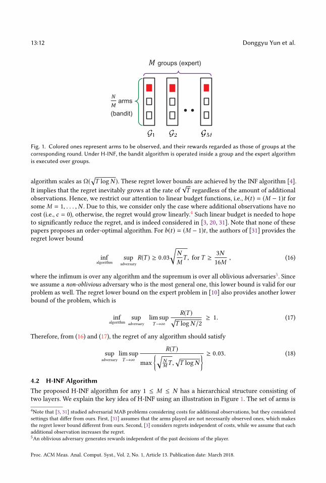
arms
(bandit)
groups (expert)
Fig. 1. Colored ones represent arms to be observed, and their rewards regarded as those of groups at thecorresponding round. Under H-INF, the bandit algorithm is operated inside a group and the expert algorithmis executed over groups.
algorithm scales as Ω(√T logN ). These regret lower bounds are achieved by the INF algorithm [4].
It implies that the regret inevitably grows at the rate of
√T regardless of the amount of additional
observations. Hence, we restrict our attention to linear budget functions, i.e., b(t) = (M − 1)t forsomeM = 1, . . . ,N . Due to this, we consider only the case where additional observations have no
cost (i.e., c = 0), otherwise, the regret would grow linearly.4Such linear budget is needed to hope
to significantly reduce the regret, and is indeed considered in [3, 20, 31]. Note that none of these
papers proposes an order-optimal algorithm. For b(t) = (M − 1)t , the authors of [31] provides theregret lower bound
inf
algorithm
sup
adversary
R(T ) ≥ 0.03
√N
MT , for T ≥
3N
16M, (16)
where the infimum is over any algorithm and the supremum is over all oblivious adversaries5. Since
we assume a non-oblivious adversary who is the most general one, this lower bound is valid for our
problem as well. The regret lower bound on the expert problem in [10] also provides another lower
bound of the problem, which is
inf
algorithm
sup
adversary
lim sup
T→∞
R(T )√T logN /2
≥ 1. (17)
Therefore, from (16) and (17), the regret of any algorithm should satisfy
sup
adversary
lim sup
T→∞
R(T )
max
√NMT ,
√T logN
≥ 0.03. (18)
4.2 H-INF AlgorithmThe proposed H-INF algorithm for any 1 ≤ M ≤ N has a hierarchical structure consisting of
two layers. We explain the key idea of H-INF using an illustration in Figure 1. The set of arms is
4Note that [3, 31] studied adversarial MAB problems considering costs for additional observations, but they considered
settings that differ from ours. First, [31] assumes that the arms played are not necessarily observed ones, which makes
the regret lower bound different from ours. Second, [3] considers regrets independent of costs, while we assume that each
additional observation increases the regret.
5An oblivious adversary generates rewards independent of the past decisions of the player.
Proc. ACM Meas. Anal. Comput. Syst., Vol. 2, No. 1, Article 13. Publication date: March 2018.
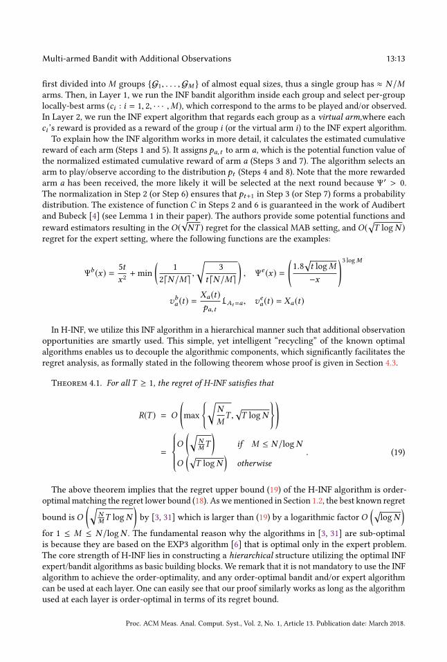
Multi-armed Bandit with Additional Observations 13:13
first divided into M groups G1, . . . ,GM of almost equal sizes, thus a single group has ≈ N /Marms. Then, in Layer 1, we run the INF bandit algorithm inside each group and select per-group
locally-best arms (ci : i = 1, 2, · · · ,M), which correspond to the arms to be played and/or observed.
In Layer 2, we run the INF expert algorithm that regards each group as a virtual arm,where eachci ’s reward is provided as a reward of the group i (or the virtual arm i) to the INF expert algorithm.
To explain how the INF algorithm works in more detail, it calculates the estimated cumulative
reward of each arm (Steps 1 and 5). It assigns pa,t to arm a, which is the potential function value of
the normalized estimated cumulative reward of arm a (Steps 3 and 7). The algorithm selects an
arm to play/observe according to the distribution pt (Steps 4 and 8). Note that the more rewarded
arm a has been received, the more likely it will be selected at the next round because Ψ′ > 0.
The normalization in Step 2 (or Step 6) ensures that pt+1 in Step 3 (or Step 7) forms a probability
distribution. The existence of function C in Steps 2 and 6 is guaranteed in the work of Audibert
and Bubeck [4] (see Lemma 1 in their paper). The authors provide some potential functions and
reward estimators resulting in the O(√NT ) regret for the classical MAB setting, and O(
√T logN )
regret for the expert setting, where the following functions are the examples:
Ψb (x) =5t
x2+min
(1
2⌈N /M⌉,
√3
t ⌈N /M⌉
), Ψe (x) =
(1.8
√t logM
−x
)3 logM
vba (t) =Xa(t)
pa,t1At=a , vea(t) = Xa(t)
In H-INF, we utilize this INF algorithm in a hierarchical manner such that additional observation
opportunities are smartly used. This simple, yet intelligent “recycling” of the known optimal
algorithms enables us to decouple the algorithmic components, which significantly facilitates the
regret analysis, as formally stated in the following theorem whose proof is given in Section 4.3.
Theorem 4.1. For all T ≥ 1, the regret of H-INF satisfies that
R(T ) = O
(max
√N
MT ,
√T logN
)
=
O
(√NMT
)if M ≤ N /logN
O(√
T logN)
otherwise. (19)
The above theorem implies that the regret upper bound (19) of the H-INF algorithm is order-
optimal matching the regret lower bound (18). As wementioned in Section 1.2, the best known regret
bound is O
(√NMT logN
)by [3, 31] which is larger than (19) by a logarithmic factor O
(√logN
)for 1 ≤ M ≤ N /logN . The fundamental reason why the algorithms in [3, 31] are sub-optimal
is because they are based on the EXP3 algorithm [6] that is optimal only in the expert problem.
The core strength of H-INF lies in constructing a hierarchical structure utilizing the optimal INF
expert/bandit algorithms as basic building blocks. We remark that it is not mandatory to use the INF
algorithm to achieve the order-optimality, and any order-optimal bandit and/or expert algorithm
can be used at each layer. One can easily see that our proof similarly works as long as the algorithm
used at each layer is order-optimal in terms of its regret bound.
Proc. ACM Meas. Anal. Comput. Syst., Vol. 2, No. 1, Article 13. Publication date: March 2018.
13:14 Donggyu Yun et al.
4.3 Proof of Theorem 4.1At the T -th round, we denote the best arm by
a⋆ = argmax
a∈NE
[T∑t=1
Xa(t)
]and the best group by G⋆
which contains a⋆. Then, it follows that
R(T ) = max
a∈NE
[T∑t=1
Xa(t)
]− E
[T∑t=1
XAt (t)
]= max
a∈G⋆E
[T∑t=1
Xa(t)
]− E
[T∑t=1
XAt (t)
]≤ max
a∈G⋆E
[T∑t=1
Xa(t)
]− E
[T∑t=1
XAt (t)
]+ max
Gi ∈G1, ...,GM E
[T∑t=1
XGi (t)
]− E
[T∑t=1
XG⋆(t)
], (20)
where XGi (t) denotes the reward of Gi at the t-th round, defined as the reward of the candidate
arm of Gi selected at Layer 1 of H-INF. We now focus on the group G⋆. One can observe that inside
the group G⋆, the algorithm runs the INF bandit algorithm over the arms in G⋆
only. Since there
are at most ⌈N /M⌉ arms in G⋆, we obtain
max
a∈G⋆E
[T∑t=1
Xa(t)
]− E
[T∑t=1
XG⋆(t)
]= O
(√⌈N /M⌉T
)= O
(√N
MT
)(21)
from the known regret bound of the INF bandit algorithm [4].6
Similarly, for Layer 2 where the INF expert algorithm is applied onM groups, we have
max
Gi ∈G1, ...,GM E
[T∑t=1
XGi (t)
]− E
[T∑t=1
XAt (t)
]= O
(√T logM
)(22)
from the known regret bound of the INF expert algorithm [4]. Therefore, combining (20), (21) and
(22) leads to
R(T ) = O
(√N
MT +
√T logM
)= O
(max
√N
MT ,
√T logN
).
This completes the proof of Theorem 4.1.
6Theorems in [4] assume that T is already known, but using the “doubling trick” in [11] can lead to the same-order regret
bound under unknown T .
Proc. ACM Meas. Anal. Comput. Syst., Vol. 2, No. 1, Article 13. Publication date: March 2018.
Multi-armed Bandit with Additional Observations 13:15
KL-UCB KL-UCB-AO KL-UCB-RRKL-UCB-CI
Reg
ret
0
50
100
Round0 100,000 200,000
(a) b(t ) = 20 log t, cost = 0
KL-UCB KL-UCB-AO KL-UCB-RRKL-UCB-CI
Reg
ret
0
50
100
Round0 100,000 200,000
(b) b(t ) = 200 log t, cost = 0
KL-UCB KL-UCB-RR KL-UCB-RRKL-UCB-CI R
egre
t
0
50
100
Round0 100,000 200,000
(c) b(t ) = t, cost = 0
KL-UCB KL-UCB-AO KL-UCB-RRKL-UCB-CI
Reg
ret
0
50
100
Round0 100,000 200,000
(d) b(t ) = 20 log t, cost = 0.1
KL-UCB KL-UCB-AO KL-UCB-RRKL-UCB-CI
Reg
ret
0
100
200
300
Round0 100,000 200,000
(e) b(t ) = 200 log t, cost = 0.1
KL-UCB KL-UCB-AO KL-UCB-RRKL-UCB-CI R
egre
t
0
200
400
Round0 100,000 200,000
(f) b(t ) = t, cost = 0.1
KL-UCB KL-UCB-AO KL-UCB-RRKL-UCB-CI
Reg
ret
0
50
100
Round0 100,000 200,000
(g) b(t ) = 20 log t, cost = 0.2
KL-UCB KL-UCB-AO KL-UCB-RRKL-UCB-CI
Reg
ret
0
200
400
Round0 100,000 200,000
(h) b(t ) = 200 log t, cost = 0.2
KL-UCB KL-UCB-AO KL-UCB-RRKL-UCB-CI R
egre
t
0
200
400
Round0 100,000 200,000
(i) b(t ) = t, cost = 0.2
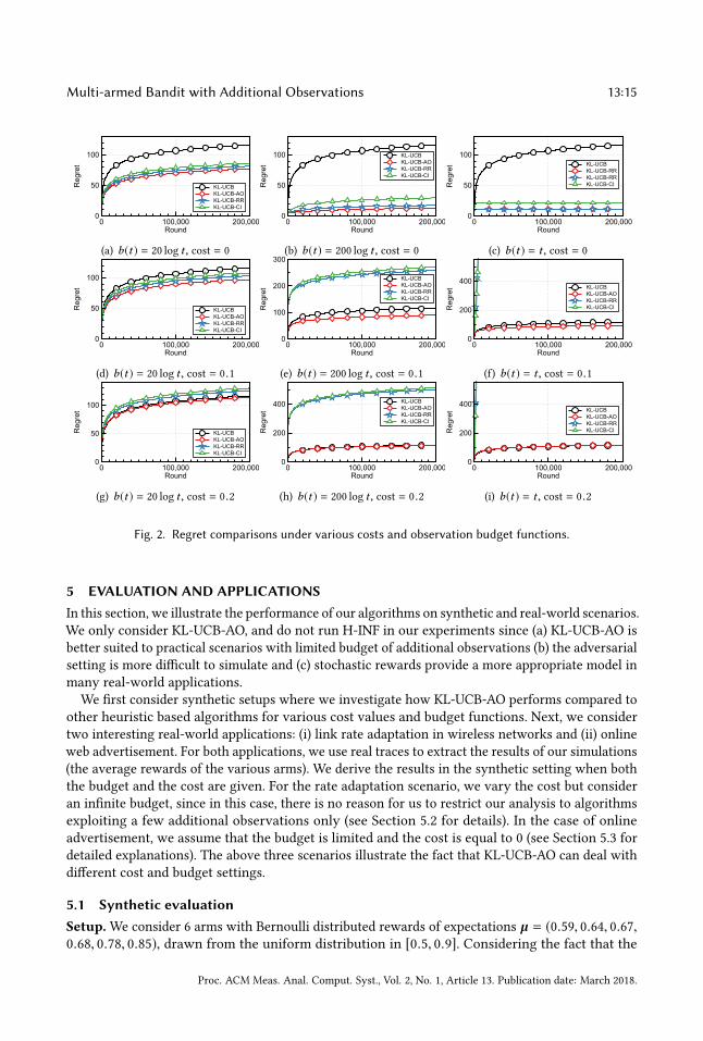
Fig. 2. Regret comparisons under various costs and observation budget functions.
5 EVALUATION AND APPLICATIONSIn this section, we illustrate the performance of our algorithms on synthetic and real-world scenarios.
We only consider KL-UCB-AO, and do not run H-INF in our experiments since (a) KL-UCB-AO is
better suited to practical scenarios with limited budget of additional observations (b) the adversarial
setting is more difficult to simulate and (c) stochastic rewards provide a more appropriate model in
many real-world applications.
We first consider synthetic setups where we investigate how KL-UCB-AO performs compared to
other heuristic based algorithms for various cost values and budget functions. Next, we consider
two interesting real-world applications: (i) link rate adaptation in wireless networks and (ii) online
web advertisement. For both applications, we use real traces to extract the results of our simulations
(the average rewards of the various arms). We derive the results in the synthetic setting when both
the budget and the cost are given. For the rate adaptation scenario, we vary the cost but consider
an infinite budget, since in this case, there is no reason for us to restrict our analysis to algorithms
exploiting a few additional observations only (see Section 5.2 for details). In the case of online
advertisement, we assume that the budget is limited and the cost is equal to 0 (see Section 5.3 for
detailed explanations). The above three scenarios illustrate the fact that KL-UCB-AO can deal with
different cost and budget settings.
5.1 Synthetic evaluationSetup.We consider 6 arms with Bernoulli distributed rewards of expectations µ = (0.59, 0.64, 0.67,0.68, 0.78, 0.85), drawn from the uniform distribution in [0.5, 0.9]. Considering the fact that the
Proc. ACM Meas. Anal. Comput. Syst., Vol. 2, No. 1, Article 13. Publication date: March 2018.
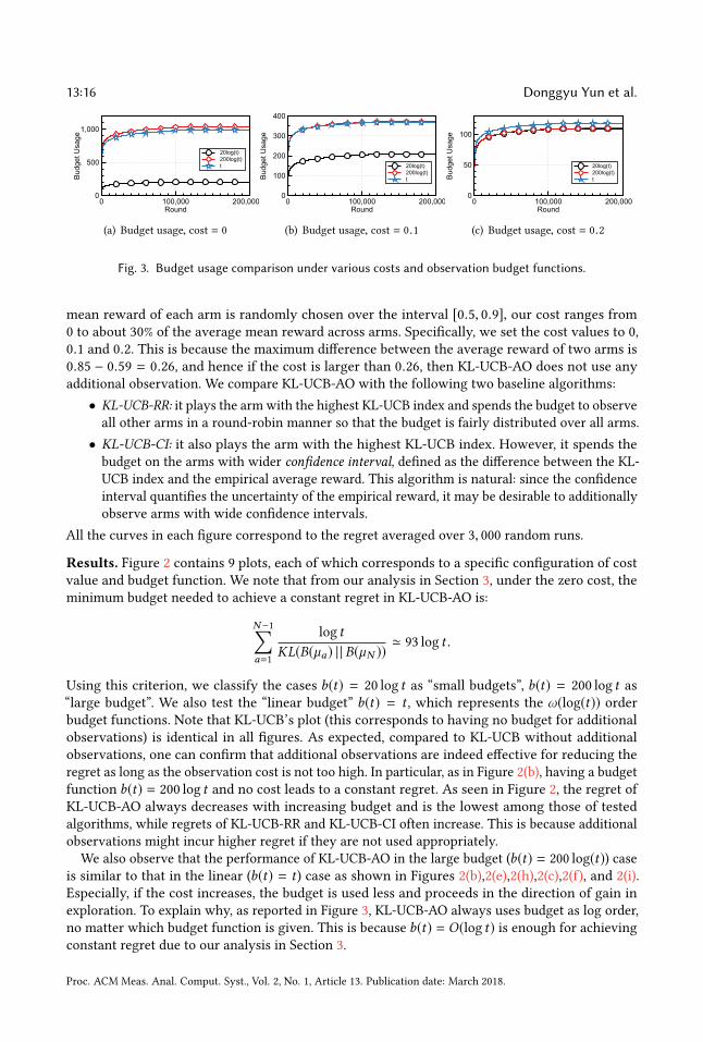
13:16 Donggyu Yun et al.
20log(t) 200log(t) t
Bud
get U
sage
0
500
1,000
Round0 100,000 200,000
(a) Budget usage, cost = 0
20log(t) 200log(t) tB
udge
t Usa
ge
0
100
200
300
400
Round0 100,000 200,000
(b) Budget usage, cost = 0.1
20log(t) 200log(t) tB
udge
t Usa
ge
0
50
100
Round0 100,000 200,000
(c) Budget usage, cost = 0.2
Fig. 3. Budget usage comparison under various costs and observation budget functions.
mean reward of each arm is randomly chosen over the interval [0.5, 0.9], our cost ranges from0 to about 30% of the average mean reward across arms. Specifically, we set the cost values to 0,
0.1 and 0.2. This is because the maximum difference between the average reward of two arms is
0.85 − 0.59 = 0.26, and hence if the cost is larger than 0.26, then KL-UCB-AO does not use any
additional observation. We compare KL-UCB-AO with the following two baseline algorithms:
• KL-UCB-RR: it plays the arm with the highest KL-UCB index and spends the budget to observe
all other arms in a round-robin manner so that the budget is fairly distributed over all arms.
• KL-UCB-CI: it also plays the arm with the highest KL-UCB index. However, it spends the
budget on the arms with wider confidence interval, defined as the difference between the KL-
UCB index and the empirical average reward. This algorithm is natural: since the confidence
interval quantifies the uncertainty of the empirical reward, it may be desirable to additionally
observe arms with wide confidence intervals.
All the curves in each figure correspond to the regret averaged over 3, 000 random runs.
Results. Figure 2 contains 9 plots, each of which corresponds to a specific configuration of cost
value and budget function. We note that from our analysis in Section 3, under the zero cost, the
minimum budget needed to achieve a constant regret in KL-UCB-AO is:
N−1∑a=1
log t
KL(B(µa) | | B(µN ))≃ 93 log t .
Using this criterion, we classify the cases b(t) = 20 log t as “small budgets”, b(t) = 200 log t as“large budget”. We also test the “linear budget” b(t) = t , which represents the ω(log(t)) orderbudget functions. Note that KL-UCB’s plot (this corresponds to having no budget for additional
observations) is identical in all figures. As expected, compared to KL-UCB without additional
observations, one can confirm that additional observations are indeed effective for reducing the
regret as long as the observation cost is not too high. In particular, as in Figure 2(b), having a budget
function b(t) = 200 log t and no cost leads to a constant regret. As seen in Figure 2, the regret of
KL-UCB-AO always decreases with increasing budget and is the lowest among those of tested
algorithms, while regrets of KL-UCB-RR and KL-UCB-CI often increase. This is because additional
observations might incur higher regret if they are not used appropriately.
We also observe that the performance of KL-UCB-AO in the large budget (b(t) = 200 log(t)) caseis similar to that in the linear (b(t) = t ) case as shown in Figures 2(b),2(e),2(h),2(c),2(f), and 2(i).
Especially, if the cost increases, the budget is used less and proceeds in the direction of gain in
exploration. To explain why, as reported in Figure 3, KL-UCB-AO always uses budget as log order,
no matter which budget function is given. This is because b(t) = O(log t) is enough for achieving
constant regret due to our analysis in Section 3.
Proc. ACM Meas. Anal. Comput. Syst., Vol. 2, No. 1, Article 13. Publication date: March 2018.
Multi-armed Bandit with Additional Observations 13:17
KL-UCB-AO ORSMiRA
RAMAS SampleRA
Aggr
egat
ed G
oodp
ut (M
bps)
0
50
100
150
0 0.2 0.4 0.6 0.8 1.0 1.2 1.4 1.6 1.8 2.0
KL-UCB-AO ORSMiRA
RAMAS SampleRA
Inst
anta
neou
s G
oodp
ut (M
bps)
0
50
100
150
Time (sec)0 0.2 0.4 0.6 0.8 1.0 1.2 1.4 1.6 1.8 2.0
(a) Stationary Channel
KL-UCB-AO ORSMiRA
RAMAS SampleRA
Aggr
egat
ed G
oodp
ut (M
bps)
0
50
100
0 5 10 15 20 25 30 35 40
KL-UCB-AO ORSMiRA
RAMAS SampleRA
Inst
anta
neou
s G
oodp
ut (M
bps)
0
50
100
150
200
Time (sec)0 5 10 15 20 25 30 35 40
(b) Non-stationary Channel, Periodical
Reset
KL-UCB-AO ORSMiRA
RAMAS SampleRA
Aggr
egat
ed G
oodp
ut (M
bps)
0
50
100
0 5 10 15 20 25 30 35 40
KL-UCB-AO ORSMiRA
RAMAS SampleRA
Inst
anta
neou
s G
oodp
ut (M
bps)
0
50
100
150
200
Time (sec)0 5 10 15 20 25 30 35 40
(c) Non-stationary Channel, Ideal Reset
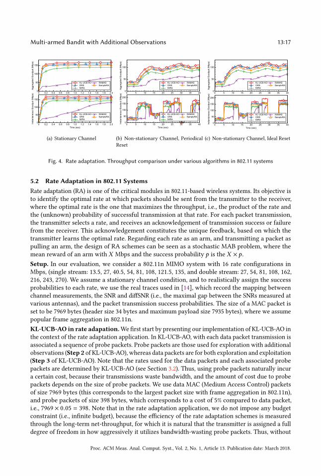
Fig. 4. Rate adaptation. Throughput comparison under various algorithms in 802.11 systems
5.2 Rate Adaptation in 802.11 SystemsRate adaptation (RA) is one of the critical modules in 802.11-based wireless systems. Its objective is
to identify the optimal rate at which packets should be sent from the transmitter to the receiver,
where the optimal rate is the one that maximizes the throughput, i.e., the product of the rate and
the (unknown) probability of successful transmission at that rate. For each packet transmission,
the transmitter selects a rate, and receives an acknowledgement of transmission success or failure
from the receiver. This acknowledgement constitutes the unique feedback, based on which the
transmitter learns the optimal rate. Regarding each rate as an arm, and transmitting a packet as
pulling an arm, the design of RA schemes can be seen as a stochastic MAB problem, where the
mean reward of an arm with X Mbps and the success probability p is the X × p.
Setup. In our evaluation, we consider a 802.11n MIMO system with 16 rate configurations in
Mbps, (single stream: 13.5, 27, 40.5, 54, 81, 108, 121.5, 135, and double stream: 27, 54, 81, 108, 162,
216, 243, 270). We assume a stationary channel condition, and to realistically assign the success
probabilities to each rate, we use the real traces used in [14], which record the mapping between
channel measurements, the SNR and diffSNR (i.e., the maximal gap between the SNRs measured at
various antennas), and the packet transmission success probabilities. The size of a MAC packet is
set to be 7969 bytes (header size 34 bytes and maximum payload size 7935 bytes), where we assume
popular frame aggregation in 802.11n.
KL-UCB-AO in rate adapation.Wefirst start by presenting our implementation of KL-UCB-AO in
the context of the rate adaptation application. In KL-UCB-AO, with each data packet transmission is
associated a sequence of probe packets. Probe packets are those used for exploration with additional
observations (Step 2 of KL-UCB-AO), whereas data packets are for both exploration and exploitation(Step 3 of KL-UCB-AO). Note that the rates used for the data packets and each associated probe
packets are determined by KL-UCB-AO (see Section 3.2). Thus, using probe packets naturally incur
a certain cost, because their transmissions waste bandwidth, and the amount of cost due to probe
packets depends on the size of probe packets. We use data MAC (Medium Access Control) packets
of size 7969 bytes (this corresponds to the largest packet size with frame aggregation in 802.11n),
and probe packets of size 398 bytes, which corresponds to a cost of 5% compared to data packet,
i.e., 7969 × 0.05 = 398. Note that in the rate adaptation application, we do not impose any budget
constraint (i.e., infinite budget), because the efficiency of the rate adaptation schemes is measured
through the long-term net-throughput, for which it is natural that the transmitter is assigned a full
degree of freedom in how aggressively it utilizes bandwidth-wasting probe packets. Thus, without
Proc. ACM Meas. Anal. Comput. Syst., Vol. 2, No. 1, Article 13. Publication date: March 2018.
13:18 Donggyu Yun et al.
the budget constraint, KL-UCB-AO behaves in such a way that it smartly controls the amount of
the probe packets over time to maximize the net-throughput computed for data packets only.
Tested algorithms for comparison.We test four baseline algorithms SampleRA [7], MiRA [29], RAMAS [28], and ORS [13] for
comparison to KL-UCB-AO. Briefly speaking, all these algorithms except for ORS heuristically use
the idea of trading exploration and exploitation in a different manner. ORS is the rate adaptation
algorithm that comes from the explicit formulation of the problem as a MAB problem, but does
not perform additional observations, relying on the pulled arm for exploration and exploitation, as
in the conventional MAB. MiRA performs additional observations via probe packets similarly to
KL-UCB-AO, where over some intervals probe packets are transmitted, with the intervals being
determined in an adaptive manner. The performance gap between MiRA and KL-UCB-AO allows us
to quantify the gain of a theory-driven optimal algorithm with additional observations. SampleRA
is the earliest version of rate adaptation in 802.11 systems, where exploration is executed every 10
packets. RMAMS is a threshold-based algorithm, where some statistics (e.g., success rate and retry
count) are checked and the selected rate is changed if those statistics are above or below some
threshold.
Results.Weperformed trace-based simulations for stationary and non-stationary channel scenarios.
We use the real traces from [14]. In the stationary scenario, the channel condition between the
transmitter and the receiver is chosen so that the maximum transmission rate is 162 Mbps. We
observe similar trends for different channel conditions. We generate non-stationary scenarios
by choosing 8 channel conditions from the traces. These conditions change at times 5, 10, 13,
20, 24, 26, 30, 36 secs. As summarized earlier, ORS corresponds to KL-UCB without additional
observations, whereas other algorithms implicitly mix exploration and exploitation in a heuristic
manner. Figure 4(a) shows the results of instantaneous (measured every 0.1 sec intervals) and
aggregate goodputs under the stationary scenario. We observe that KL-UCB-AO finds the optimal
rate slightly faster than ORS, and that other algorithms perform sub-optimally. This result illustrates
the fact that additional observations enable to dynamically utilize exploration chances so that the
optimal arm is quickly found. The advantage of additional observations becomes even clearer in
the non-stationary scenario. Figures 4(b) and 4(c) show the gootputs when the learning algorithms
are periodically and ideally reset, respectively. By ideally, we mean that the transmitter magically
knows when the channel condition changes and resets its parameters in the algorihtms. These two
ways of ‘periodic and ideal reset’ are just the baseline mechanisms that respond to non-stationary
condition changes, and developing a better mechanism is beyond the scope of this paper. However,
we are able to quantify how beneficial the idea of using additional observations like KL-UCB-AO is,
compared to those without it. In Figures 4(b) and 4(c), we observe that KL-UCB-AO achieves the
goodputs of upto 50 Mbps higher than other algorithms, and overall it quickly finds the optimal
rate and thus achieves larger goodputs over time.
5.3 Online AdvertisementOnline advertisement is one of the major income sources for the Internet industry today [18]. An
advertiser who wants to promote new products would buy an ad placement on a popular website.
Whenever a user visits the website, the web administrator should choose a few ads to display
among many candidate ones. For example, in case of sponsored advertising [18] in a search engine
such as Google, an advertiser bids for keywords related to her product or service to display her ad.
For example, car manufacturers might want to advertise their products when the keyword ‘car’ isqueried. In this case, the search engine should display an ad among those of car manufacturers
that actually bid for the keyword. It should select the ad with the highest click-through-rate
Proc. ACM Meas. Anal. Comput. Syst., Vol. 2, No. 1, Article 13. Publication date: March 2018.
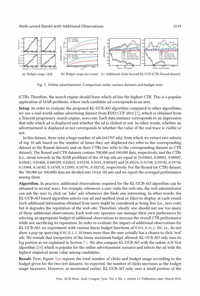
Multi-armed Bandit with Additional Observations 13:19
Budg
et U
sage
(%)
0%
5%
10%
15%
1% 10% 100% 1000%
Tota
l Clic
ks (%
)
49.5%
50.0%
50.5%
51.0%
51.5%
Max Budget (%) - CTR Dataset1% 10% 100% 1,000%
0%
5%
10%
1% 10% 100% 1000%
8.9%
9.0%
9.1%
9.2%
9.3%
Max Budget (%) - Round Dataset1% 10% 100% 1000%
(a) Budget usage, click
Budg
et U
sage
(%)
10% Budget100% Budget 1000% Budget
CTR
Dat
aset
0%
5%
10%
15%
0 2000 4000 6000
10% Budget100% Budget 1000% Budget
Rou
nd D
atas
et
0%
5%
10%
15%
Round0 10,000 20,000 30,000
(b) Budget usage per round
A/B Test 1% (Usage 0.18%) 10% (Usage 2.88%)100% (Usage 11.00%) 1000% (Usage 16.26%)
Addi
tiona
l Clic
ks
−400
−300
−200
−100
0
100
200
300
Round - CTR Dataset0 2000 4000 6000
A/B Test 1% (Usage 0.10%) 10% (Usage 2.24%)100% (Usage 7.93%) 1000% (Usage 13.18%)
−400
−300
−200
−100
0
100
200
300
Round - Round Dataset0 10,000 20,000 30,000
(c) Additional clicks beyond KL-UCB (CTR, Round dataset)
Fig. 5. Online advertisement. Comparison under various datasets and budget sizes
(CTR). Therefore, the search engine should learn which ad has the highest CTR. This is a popular
application of MAB problems, where each candidate ad corresponds to an arm.
Setup. In order to evaluate the proposed KL-UCB-AO algorithm compared to other algorithms,
we use a real-world online advertising dataset from KDD CUP 2012 [1], which is obtained from
a Tencent proprietary search engine, soso.com. Each data instance corresponds to an impression
that tells which ad is displayed and whether the ad is clicked or not. In other words, whether an
advertisement is displayed or not corresponds to whether the value of the real trace is visible or
not.
In this dataset, there exist a huge number of ads (641707 ads), from which we extract two subsets
of top 10 ads based on the number of times they are displayed (we refer to the corresponding
dataset as the Round dataset) and on their CTRs (we refer to the corresponding dataset as CTR
dataset). The Round and CTR datasets contain 700,000 and 100,000 data, respectively, and the CTRs
(i.e., mean rewards in the MAB problem) of the 10 top ads are equal to [0.05065, 0.00001, 0.00007,
0.03681, 0.03468, 0.000189, 0.02023, 0.03158, 0.0101, 0.08369] and [0.45514, 0.31748, 0.29142, 0.19736,
0.15904, 0.14182, 0.14768, 0.12895, 0.10791, 0.10273], respectively. For the Round (or CTR) dataset,
the 700,000 (or 100,000) data are divided into 14 (or 10) sets and we report the averaged performance
among them.
Algorithm. In practice, additional observations required for the KL-UCB-AO algorithm can be
obtained in several ways. For example, whenever a user visits the web-site, the web administrator
can ask the user to click on ‘fake’ ads whenever she finds one interesting. In other words, the
KL-UCB-AO based algorithm selects one ad and method (real or fake) to display at each round.
Such additional information obtained from users might be considered as being free (i.e., zero cost),
but it degrades the reputation of the web-site. Therefore, ideally one should not use too many
of these additional observations. Each web-site operator can manage their own preferences by
selecting an appropriate budget of additional observations to increase the overall CTR performance
while not sacrificing its reputation. In order to evaluate the impact of additional observations for
KL-UCB-AO, we experiment with various linear budget functions of 0.01t , 0.1t , t , 10t , i.e., do not
show a pop-up querying 0.01, 0.1, 1, 10 times more than the user actually has a chance to click ‘real’
ads. We remark that irrespective of the linear maximum budget allowed, KL-UCB-AO only uses its
log portion as we explained in Section 5.1. We also compare KL-UCB-AO with the online A/B Test
algorithm [24] which is popular for the online advertisement scenario and selects the ad with the
highest empirical mean value among candidates.
Result. First, Figure 5(a) reports the total number of clicks and budget usage according to the
budget given for the two test datasets. As expected, the number of clicks increases as the budget
usage increases. However, as mentioned earlier, KL-UCB-AO only uses a small portion of the
Proc. ACM Meas. Anal. Comput. Syst., Vol. 2, No. 1, Article 13. Publication date: March 2018.
13:20 Donggyu Yun et al.
maximum budget allowed for additional observations. Second, Figure 5(b) shows the pattern of
actual budget usage per round. Even if the budget is linearly increasing with time, additional
observations are used a sub-linear (i.e., log) number of times. Third, 5(c) represents the number
of additional clicks achieved by KL-UCB-AO and A/B Test compared to that by KL-UCB, which
quantifies the advertisement gain achieved thanks to additional observations. As reported in 5(c),
the total number of clicks under KL-UCB-AO achieves the best performance. Overall, we observe
that additional observations lead to up to 4 ∼ 5% improvement in terms of the total number of
clicks.
6 CONCLUSIONIn this paper, we studied the multi-armed bandit with additional observations which provides a
natural extension between the bandit problem and the expert problem. For stochastic rewards, we
derive an asymptotic lower bound on regret, satisfied by any uniformly good algorithm. Motivated
by the lower bound, we developed KL-UCB-AO, an asymptotically optimal algorithm. For adversarial
rewards, we propose a hierarchical algorithm whose regret is order-optimal. We present two
applications in rate adaptation over wireless networks and online advertisement, where we showed
the proposed algorithms’ value in practice. We believe that our ideas in designing bandit algorithms
are of boarder interest to study similar problems, e.g., the contextual or graph-structured bandit
problems.
ACKNOWLEDGMENTSThe work of Y. Yi is supported by Basic Science Research Program through the National Research
Foundation of Korea(NRF) funded by the Ministry of Science and ICT(No. 2016R1A2A2A05921755).
The work of A. Proutiere is supported by the ERC consolidator grant 308267 - Fluid SpectrumAccess,
by VR, and SRA TNG framework. The work of J.W. Shin is supported by the ICT R&D program of
MSIP/IITP. [2016-0-00563, Research on Adaptive Machine Learning Technology Development for
Intelligent Autonomous Digital Companion]
REFERENCES[1] KDD cup 2012 Track 2. http://www.kddcup2012.org/c/kddcup2012-track2.
[2] Noga Alon, Nicolo Cesa-Bianchi, Claudio Gentile, and Yishay Mansour. 2013. From bandits to experts: A tale of
domination and independence. In Proceedings of NIPS.[3] Kareem Amin, Satyen Kale, and Gerald Tesauro Deepak Turaga. 2015. Budgeted Prediction With Expert Advice. In
Proceedings of AAAI.[4] Jean-Yves Audibert and Sébastien Bubeck. 2010. Regret bounds and minimax policies under partial monitoring. The
Journal of Machine Learning Research 11 (2010), 2785–2836.
[5] P. Auer, N. Cesa-Bianchi, and P. Fischer. 2002. Finite time analysis of the multiarmed bandit problem. Machine Learning47, 2-3 (2002), 235–256.
[6] Peter Auer, Nicolò Cesa-Bianchi, Yoav Freund, and Robert E. Schapire. 2002. The nonstochastic multiarmed bandit
problem. SIAM J. Comput. 32, 1 (2002), 48–77.[7] J. Bicket. 2005. Bit-rate selection in wireless networks. In PhD thesis, Massachusetts Institute of Technology.[8] Swapna Buccapatnam, Atilla Eryilmaz, and Ness B Shroff. 2014. Stochastic bandits with side observations on networks.
In Proceedings of ACM SIGMETRICS.[9] Stéphane Caron, Branislav Kveton, Marc Lelarge, and Smriti Bhagat. 2012. Leveraging Side Observations in Stochastic
Bandits. In Proceedings of UAI.[10] Nicolo Cesa-Bianchi, Yoav Freund, David Haussler, David P Helmbold, Robert E Schapire, and Manfred K Warmuth.
1997. How to use expert advice. Journal of the ACM (JACM) 44, 3 (1997), 427–485.[11] Nicolò Cesa-Bianchi and Gábor Lugosi. 2006. Prediction, Learning, and Games. Cambridge University Press.
[12] Richard Combes, Chong Jiang, and R Srikant. 2015. Bandits with Budgets: Regret Lower Bounds and Optimal Algorithms.
In Proceedings of ACM SIGMETRICS.
Proc. ACM Meas. Anal. Comput. Syst., Vol. 2, No. 1, Article 13. Publication date: March 2018.
Multi-armed Bandit with Additional Observations 13:21
[13] Richard Combes, Alexandre Proutiere, Donggyu Yun, Jungseul Ok, and Yung Yi. 2014. Optimal rate sampling in 802.11
systems. In Proceedings of IEEE INFOCOM.
[14] L. Deek, E. Garcia-Villegas, E. Belding, S.-J. Lee, and K. Almeroth. 2013. Joint rate and channel width adaptation in
802.11 MIMO wireless networks. In Proceedings of IEEE SECON.[15] P. Frazier, D. Kempe, J. Kleinberg, and R. Kleinberg. 2014. Incentivizing exploration. In Proceedings of the fifteenth ACM
conference on Economics and computation. 5–22.[16] Yoav Freund and Robert E Schapire. 1997. A decision-theoretic generalization of on-line learning and an application to
boosting. Journal of computer and system sciences 55, 1 (1997), 119–139.[17] A. Garivier and O. Cappé. 2011. The KL-UCB algorithm for bounded stochastic bandits and beyond. In Proceedings of
COLT.[18] Thore Graepel, Joaquin Q Candela, Thomas Borchert, and Ralf Herbrich. 2010. Web-scale bayesian click-through rate
prediction for sponsored search advertising in microsoft’s bing search engine. In Proceedings of the 27th InternationalConference on Machine Learning (ICML-10).
[19] Adam Kalai and Santosh Vempala. 2005. Efficient algorithms for online decision problems. J. Comput. System Sci. 71, 3(2005), 291–307.
[20] Satyen Kale. 2014. Multiarmed bandits with limited expert advice. In Proceedings of COLT.[21] Emilie Kaufmann, Olivier Cappé, and Aurélien Garivier. 2012. On Bayesian upper confidence bounds for bandit
problems. In Proceedings of AISTATS.[22] Emilie Kaufmann, Olivier Cappé, and Aurélien Garivier. 2016. On the Complexity of Best Arm Identification in
Multi-Armed Bandit Models. The Journal of Machine Learning Research 17 (2016), 1–42.
[23] Tomáš Kocák, Gergely Neu, Michal Valko, and Remi Munos. 2014. Efficient learning by implicit exploration in bandit
problems with side observations. In Proceedings of NIPS.[24] Ron kohavi. 2015. Online Controlled Experiments: Lessons from Running A/B/N Tests for 12 Years. In Proceedings of
the 21th ACM SIGKDD International Conference on Knowledge Discovery and Data Mining.[25] T.L. Lai and H. Robbins. 1985. Asymptotically efficient adaptive allocation rules. Advances in Applied Mathematics 6, 1
(1985), 4–2.
[26] Shie Mannor and Ohad Shamir. 2011. From bandits to experts: On the value of side-observations. In Proceedings ofNIPS.
[27] Y. Mansour, A. Slivkins, and V. Syrgkanis. 2015. Bayesian incentive-compatible bandit exploration. In Proceedings ofthe Sixteenth ACM Conference on Economics and Computation. 565–582.
[28] J. Garcia N. Duy. 2011. A practical approach to rate adaptation for multi-antenna systems. In Proceedings of 19th IEEEInternational Conference on Network Protocols. 331–340.
[29] Ioannis Pefkianakis, Yun Hu, Starsky HY Wong, Hao Yang, and Songwu Lu. MIMO rate adaptation in 802.11n wireless
networks. In proceedings of ACM Mobicom.
[30] Herbert Robbins. 1952. Some aspects of the sequential design of experiments. Bull. Amer. Math. Soc. 58, 5 (1952),527–535.
[31] Yevgeny Seldin, Peter Bartlett, Koby Crammer, and Yasin Abbasi-Yadkori. 2014. Prediction with Limited Advice and
Multiarmed Bandits with Paid Observations. In Proceedings of ICML.[32] Yevgeny Seldin, Koby Crammer, and Peter Bartlett. 2013. Open Problem: Adversarial Multiarmed Bandits with Limited
Advice. In Proceedings of COLT.[33] Aleksandrs Slivkins, Filip Radlinski, and Sreenivas Gollapudi. 2013. Ranked bandits in metric spaces: learning diverse
rankings over large document collections. The Journal of Machine Learning Research 14, 1 (2013), 399–436.
[34] Min Xu, Tao Qin, and Tie-Yan Liu. 2013. Estimation Bias in Multi-Armed Bandit Algorithms for Search Advertising. In
Proceedings of NIPS.
Proc. ACM Meas. Anal. Comput. Syst., Vol. 2, No. 1, Article 13. Publication date: March 2018.
13:22 Donggyu Yun et al.
APPENDIX A: REGRET LOWER BOUNDFor the sake of completeness, we provide a more detailed proof of (1), following the arguments
in [22] to prove Theorem 21. Let a , N be a suboptimal arm. Let us do the following change-
of-measure: consider a new reward vector µ = (µ1, . . . , µa−1, µ, µa+1, . . . , µN ) in which only µa is
replaced by µ, where µN < µ < 1. Hence, the arm a becomes the unique optimal arm under µ.Denote by ZT the set of observations up to time T (the arms selected and their observed rewards
up to time T ), and by FT = σ (ZT ) the corresponding σ -algebra. Further denote by L = log(Pµ [ZT ]Pµ [ZT ]
)
the log-likelihood ratio of ZT under Pµ and Pµ . Then, by changing the measure from Pµ to Pµ , weget (see Lemma 18 in [22]): for all E ∈ FT ,
Pµ[E] = Eµ[1E exp(−L)].
Now applying Wald lemma and the data processing inequality, we obtain (see Lemma 19 in [22]):
Eµ[L] = Eµ[Oa(T )]KL(µa ∥ µ) ≥ KL(Pµ[E] ∥ Pµ[E]).
Now select E = AN (T ) ≤ T −√T . Markov inequality yields:
Pµ[E] = Pµ[T −AN (T ) ≥√T ] ≤
∑a,N Eµ[Aa(T )]
√T
Pµ[Ec ] ≤
Eµ[AN (T )]
T −√T
≤
∑j,a Eµ[Aj (T )]
T −√T
Since the algorithm is uniformly good, we must have for all α > 0,
∑a,N Eµ[Aa(T )] = o(T
α ) and∑j,a Eµ[Aj (T )] = o(T
α ). Hence Pµ[E] → 0 and Pµ[E] → 1 as T → ∞. We conclude that:
KL(Pµ[E] ∥ Pµ[E])
log(T )T→∞∼
1
log(T )log(
1
Pµ[Ec ])
≥1
log(T )log(
T −√T∑
j,a Eµ[Aj (T )]).
The r.h.s. of the latter inequality is 1 + o(1) since again the algorithm is uniformly good. We have
proved that:
lim inf
T→∞
Eµ[Oa(T )]
log(T )≥
1
KL(µa ∥ µ).
Inequality (1) is obtained by letting µ tend to µ⋆.
Proc. ACM Meas. Anal. Comput. Syst., Vol. 2, No. 1, Article 13. Publication date: March 2018.