Embed Size (px)
Citation preview
The Mistake of 1937: A General Equilibrium Analysis
April 2006
— preliminary —
Gauti B. Eggertsson, Federal Reserve Bank of New York
Benjamin Pugsley, Federal Reserve Bank of New York
http://www.ny.frb.org/research/economists/eggertsson/index.html
Abstract
This paper studies a dynamic general equilibrium model with sticky prices and rational expectations in
an environment of low interest rates and deflationary pressures. We show that small changes in the public’s
beliefs about the future inflation target of the government can lead to large swings in both inflation
and output. This effect is much larger at low interest rates than under regular circumstances. This
highlights the importance of effective communication policy at zero interest rates. We argue that confusing
communications by the US Federal Reserve, the President of the United States, and key administration
officials about future price objectives were responsible for the sharp recession in the US in 1937-38, one of
the sharpest recessions in US economic history. Poor communication policy is the mistake of 1937. Before
committing the mistake of 1937 the US policy makers faced economic conditions that are similar in some
respect to those confronted by Japanese policy makers in the first half of 2006.
__________________
The views expressed are those of the authors and do not reflect those of the Federal Reserve Bank of
New York or the Federal Reserve System. We thank Mike Woodford for discussion.
1
1 Introduction
The economic conditions can be summarized as follows: 1) There are signs that the depression is finally
over. 2) Interest rates have been close to zero for years but are now finally expected to rise. 3) There are
some concerns from both policymakers and the market participants over indications of excessive inflation.
4) This is of particular concern to some who point to a large expansion in the monetary base in the past
several years as well as the current bank holdings of large excess reserves.
These four conditions characterize the economic outlook of the United States in the early months of 1937
at the precipice of one of the most peculiar policy mistakes in US economic history. These circumstances
may sound familiar to Japanese audience. In some respects Japanese policymakers confront the same
problems. How should one manage monetary policy in a transition phase from zero short-term interest
rate and deflationary pressures back to more normal circumstances? We want to emphasize right from
the start, however that fortunately it seems that both the Bank of Japan and the Japanese government
have not committed any mistakes of the same order as observed 1937. Yet, it is useful to understand the
circumstances and mechanics of the US mistake as a precautionary tale for both current and future policy
makers.
This paper addresses the "mistake of 1937", which reversed the tide of the recovery from the Great
Depression in 1933-37 into a short but sharp recession from 1937-38. Between May of 1937 and June of
1938 GDP contracted by 9 percent1 and industrial production by 40 percent. The general price level took
a tumble as well. The index of wholesale prices, for example, fell by more than 11 percent, several leading
commodity prices collapsed and the stock market lost almost half of its value.
The mistake of 1937 was in essence a poor communications policy. At the time, President Franklin
Delano Roosevelt (FDR), his administration, and the Federal Reserve all offered confusing signals about
the objectives of government policy, especially as it related to their goals for inflation. These vague and
confusing signals about future policy created pessimistic expectations of future growth and price inflation
that fed into both an expected and an actual deflation. Nominal rigidities helped propagate these impulses
into a full scale recession. We show that this propagation mechanism is particularly damaging at zero
interest rates by constructing a stylized stochastic general equilibrium model in which the zero bound on
short-term interest rate is binding due to temporary shocks. We simulate this model and show that at
zero interest rates, both inflation and output are extremely sensitive to signals about future policy. By
"extremely" we mean that if the public’s beliefs about the probability of a future regime change by only
a few percentage points, there are very large effects on inflation and output. This effect is independent of
any change in the current short-term interest rate, which we assume remains at zero.
In this stylized model, an example of such an effect might read as follows: Suppose the public fully
believes that the government is committed to targeting 4 percent inflation. Now assume that in response
to recent coverage in the press that the public thinks that there is a five percent chance that the government
will change its goals of 4 percent inflation in favor of a zero inflation goal within the next two years. This
small change in beliefs in our calibrated model results in double digit output collapse and deflation. The
large effects of shifting public beliefs about future policy may help explain how the vague and confusing
communications in 1937, which we document in some detail, had such a large negative impact.
1We use quarterly estimates of real and nominal gross national product from Barger and Klein, which are archived in theNBER Macrohistory database series q08296a q08260a respectively.
2
We find that the effect of communication is highly non-linear at zero interest rates. At zero interest
rates, the marginal effect of creating deflationary expectation by signaling tightening (targeting lower future
inflation) is much larger than the marginal effect of signaling loosening of policy (targeting higher inflation).
Our interpretation of this finding is that if a policy maker is uncertain about the nature of the real shocks
and wishes to be conservative he should err on the side of allowing some excess inflation.
The large effect of communication, and this peculiar asymmetry, is unique to an environment in which
the short-term interest rate is zero. The reason is that this environment is susceptible to what we term
deflationary spirals. The dynamics of the deflationary spirals are that if the public expects a more defla-
tionary regime in the future, this expectation creates deflationary expectations in all future states of the
world in which interest rate are zero (i.e. when the zero bound on the short term interest rate is binding).
Those states of the world, in turn, depend on each other and they create a vicious feedback effect that may
not even converge to a bounded solution (for some parameter values) in the approximated solution of our
model.
Because our theory relies on shifting public beliefs about future policy, a natural place to look for
evidence for the theory is within the newspapers in 1937-38. In the next subsection we document several
narrative newspaper accounts that are consistent with our hypothesis. In addition we construct a new index
based on newspaper records which summarizes the intensity of communication policy at a given time. We
find evidence of a ahrf increase in policy communcation in the months we identify with the mistake of 1937.
Our theory gives a novel account of the mechanism by which monetary policy was responsible for the
recession of 1937 and the recovery in 1938. Previous accounts of monetary policy during this period, e.g.
Friedman and Schwartz (1963), Romer (1992) and Meltzer (2003), have mostly focused on static changes in
some measure of the money supply and static changes (or rather lack there of) in the short-term nominal
interest rate which only increased temporarily in 1937 and then only by very modest amounts. The current
paper differs from most studies of monetary policy during this period because according to our model
the evolution of monetary aggregates is completely irrelevant at zero interest rates, except in their role in
influencing the expectations about future money supply at the time at which the interest rates are expected
to be positive.
Our view is that the expectation channel strengthens the argument made by the authors cited above,
among others, that monetary factors were responsible for the contraction of 1937-38. Furthermore, our
theory is less subject to some of the traditional Keynesian objections which we discuss in some detail in
the next section. Much of the Keynesian literature maintains that increasing the money supply, and by
implication any monetary policy, is irrelevant due to the zero bound on the short-term interest rate. While
the current model shares the zero bound with the Keynesian literature, monetary policy still exerts a very
strong effect on economic outcomes because expectations about future money supply have a large effect on
output and prices.
This paper builds on recent advances in the analysis of stochastic general equilibrium models with
nominal frictions at zero interest rates. Recent paper in this vain include Krugman (1998), Jung, Teren-
ishi, Watanabe (2001), Svensson (2001,2003), Jeanne and Svensson (2004), Eggertsson and Woodford
(2003,2004), Christiano, Motto and Rostagno (2004), Auerbach and Obstfeld (2005), Eggertsson (2005,
2006a,b), Adam and Billi (2006a,b) and Nakov (2006). For an excellent survey of some of this literature
see Svensson (2004) and for a short summary see Eggertsson (2006c). The paper shares with this work
its emphasis on the importance of expectations about future policy when interest rates are zero. It adds
3
to this literature by modeling shifts in expectations as being due to a Markov switching process for policy
regimes. This innovation allows us to simulate to model to replicate the Great Depression and gives a novel
account of the depression of 1937-38 as being due to shift in beliefs about future money supply rather than
due to static changes in the money supply, which this literature has shown to be irrelevant at zero interest
rates.
2 Historical Narrative: The Great Depression in the US and the
Mistake of 1937
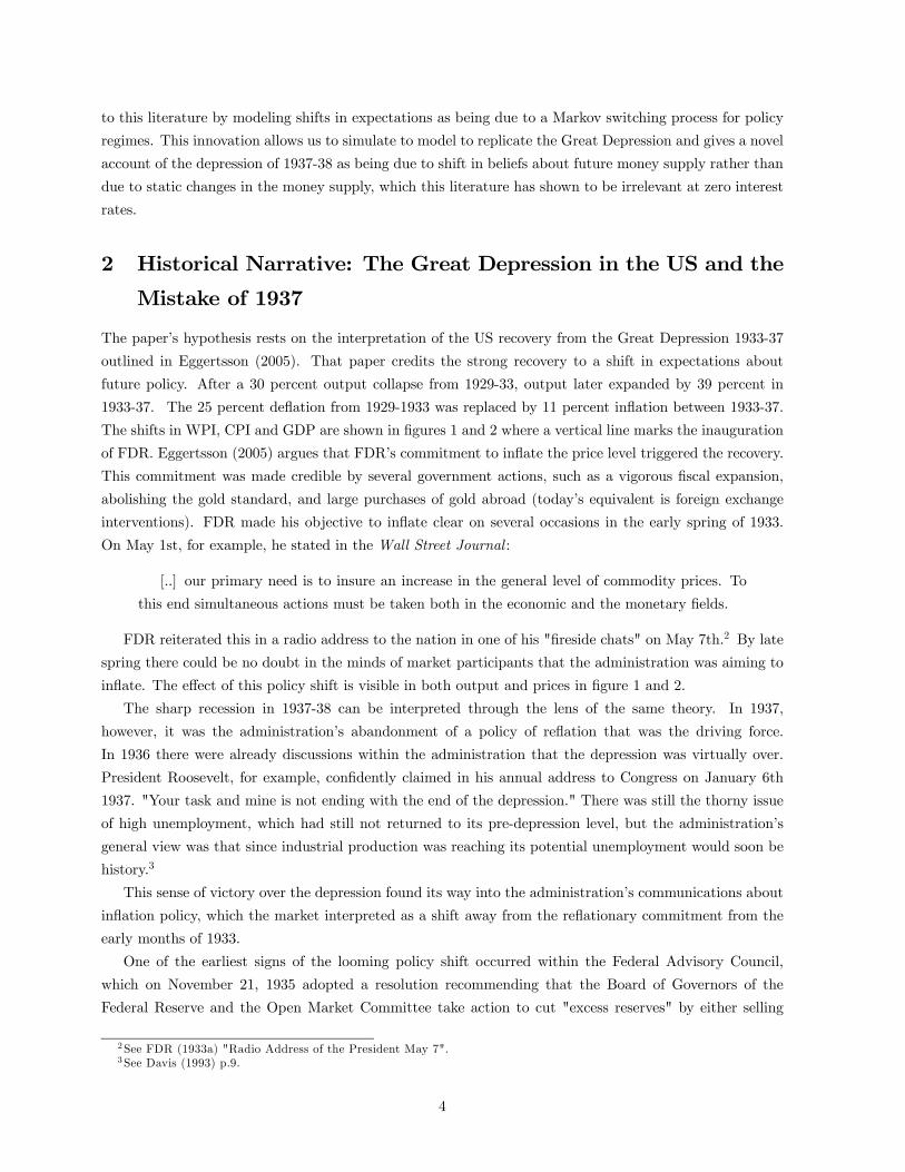
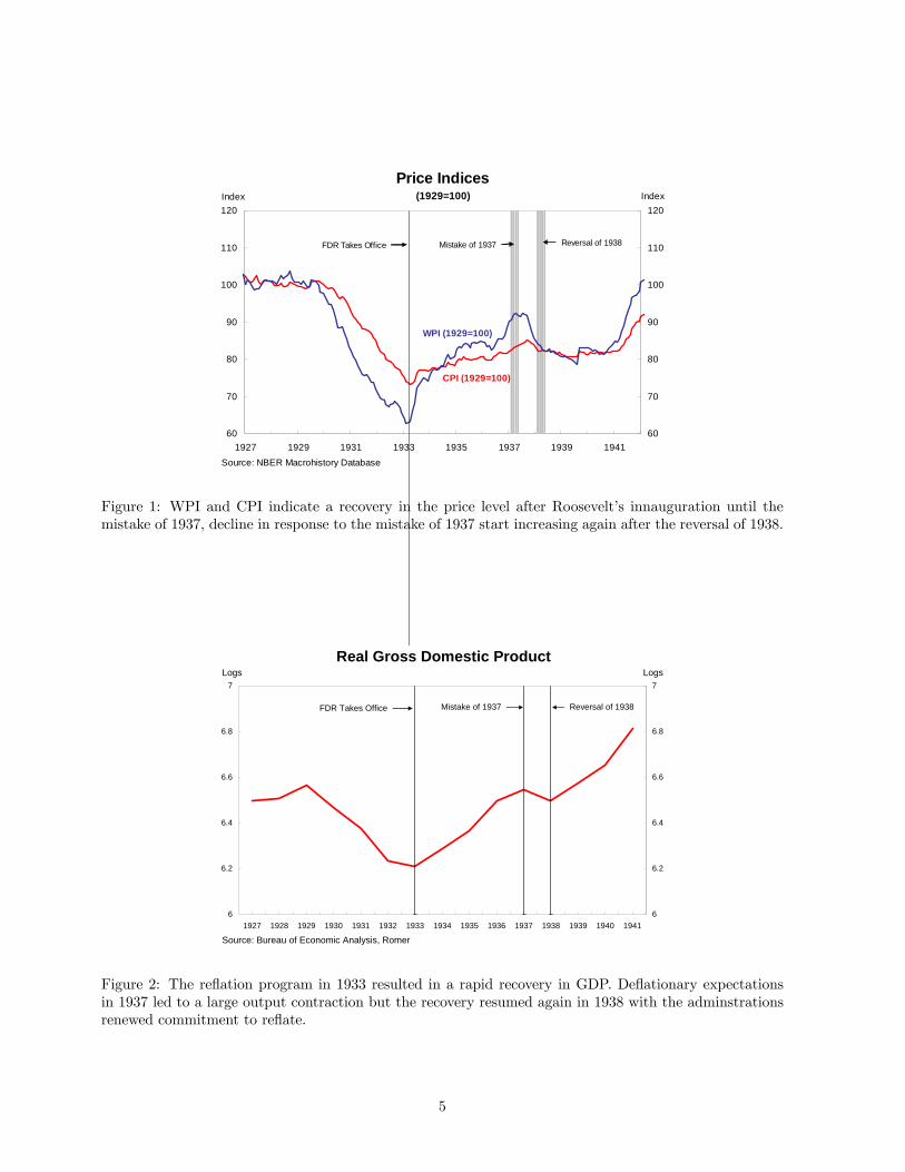
The paper’s hypothesis rests on the interpretation of the US recovery from the Great Depression 1933-37
outlined in Eggertsson (2005). That paper credits the strong recovery to a shift in expectations about
future policy. After a 30 percent output collapse from 1929-33, output later expanded by 39 percent in
1933-37. The 25 percent deflation from 1929-1933 was replaced by 11 percent inflation between 1933-37.
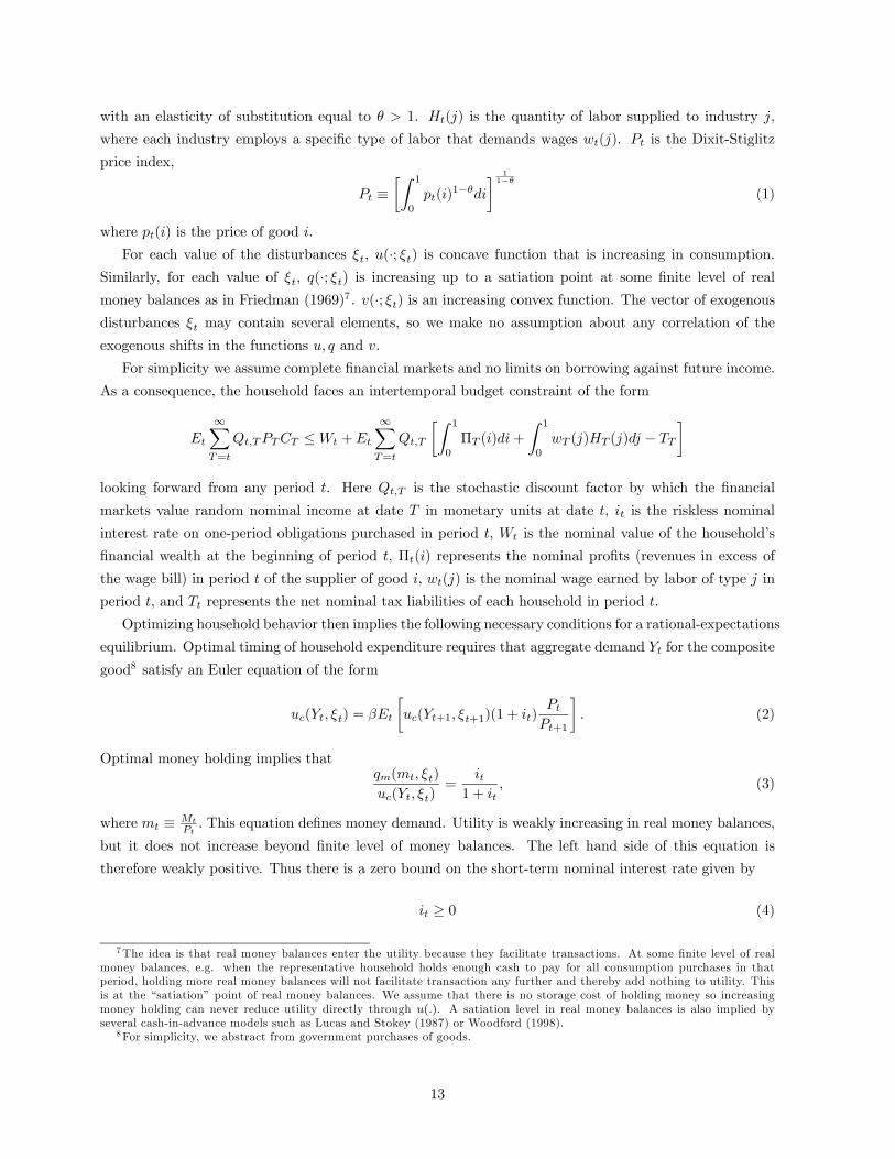
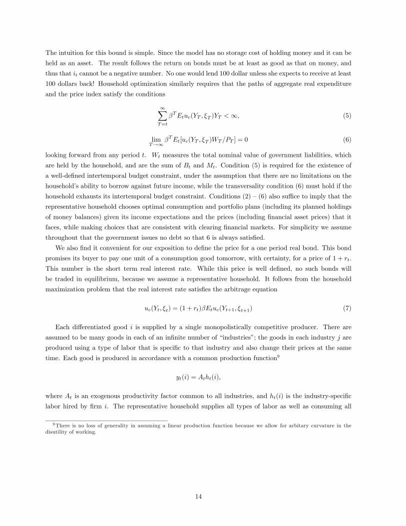
The shifts in WPI, CPI and GDP are shown in figures 1 and 2 where a vertical line marks the inauguration
of FDR. Eggertsson (2005) argues that FDR’s commitment to inflate the price level triggered the recovery.
This commitment was made credible by several government actions, such as a vigorous fiscal expansion,
abolishing the gold standard, and large purchases of gold abroad (today’s equivalent is foreign exchange
interventions). FDR made his objective to inflate clear on several occasions in the early spring of 1933.
On May 1st, for example, he stated in the Wall Street Journal :
[..] our primary need is to insure an increase in the general level of commodity prices. To
this end simultaneous actions must be taken both in the economic and the monetary fields.
FDR reiterated this in a radio address to the nation in one of his "fireside chats" on May 7th.2 By late
spring there could be no doubt in the minds of market participants that the administration was aiming to
inflate. The effect of this policy shift is visible in both output and prices in figure 1 and 2.
The sharp recession in 1937-38 can be interpreted through the lens of the same theory. In 1937,
however, it was the administration’s abandonment of a policy of reflation that was the driving force.
In 1936 there were already discussions within the administration that the depression was virtually over.
President Roosevelt, for example, confidently claimed in his annual address to Congress on January 6th
1937. "Your task and mine is not ending with the end of the depression." There was still the thorny issue
of high unemployment, which had still not returned to its pre-depression level, but the administration’s
general view was that since industrial production was reaching its potential unemployment would soon be
history.3
This sense of victory over the depression found its way into the administration’s communications about
inflation policy, which the market interpreted as a shift away from the reflationary commitment from the
early months of 1933.
One of the earliest signs of the looming policy shift occurred within the Federal Advisory Council,
which on November 21, 1935 adopted a resolution recommending that the Board of Governors of the
Federal Reserve and the Open Market Committee take action to cut "excess reserves" by either selling
2See FDR (1933a) "Radio Address of the President May 7".3 See Davis (1993) p.9.
4
60
70
80
90
100
110
120
1927 1929 1931 1933 1935 1937 1939 194160
70
80
90
100
110
120
Price Indices
Source: NBER Macrohistory Database
CPI (1929=100)
(1929=100)Index Index
WPI (1929=100)
FDR Takes Office Mistake of 1937 Reversal of 1938
Figure 1: WPI and CPI indicate a recovery in the price level after Roosevelt’s innauguration until themistake of 1937, decline in response to the mistake of 1937 start increasing again after the reversal of 1938.
6
6.2
6.4
6.6
6.8
7
1927 1928 1929 1930 1931 1932 1933 1934 1935 1936 1937 1938 1939 1940 19416
6.2
6.4
6.6
6.8
7
Source: Bureau of Economic Analysis, Romer
Real Gross Domestic ProductLogs Logs
FDR Takes Office Mistake of 1937 Reversal of 1938
Figure 2: The reflation program in 1933 resulted in a rapid recovery in GDP. Deflationary expectationsin 1937 led to a large output contraction but the recovery resumed again in 1938 with the adminstrationsrenewed commitment to reflate.
5
some portion of their government securities holdings or by raising member bank reserve requirements.
The Board ignored these recommendations until midsummer of 1936 when the Board scheduled a raise in
reserve requirements, to become effective on August 15th in 1936.
This action appears to have had a rather limited effect on markets because it was not associated with
an explicit objective to reduce inflation. Indeed the Federal Reserve generally presented the increase in the
reserve requirements as having no immediate effect and as being "harmless." The Fed agreed in January
1937 to a second round of increases to be scheduled for March and May of that year, and again the
reaction of the market was muted. In the ensuing months, however, things began to change. Newspaper
accounts of that period indicate that in February, March, and April there was increasing alarm within the
administration of the threat of excessive inflation. Some pointed to the large increases in the monetary
base over the period 1933-37 as evidence of this danger. This fear also started influencing how government
officials communicated policy, in particular they no longer presented the increase in the reserve requirement
as being purely mechanical or "harmless". On February 17th, Marriner Eccles, the Chairman of the Fed,
said in the Wall Street Journal, that "the short-term rates are excessively low and there may be a tendency
for rates near the vanishing point to increase." Furthermore he suggested that the reserve requirements
were also likely to cause an increase in long-term interest rates. The Wall Street Journal commented on
this statement on the 18th of February 1937. "This is the first time a member of the board has publicly
described the reserve requirement as a device for preventing a further drop in long time rates." About one
month later Fed Chairman Marriner Eccles called upon the Treasury to fight against "excessive" inflation
by balancing the budget.4
This and other newspaper accounts indicate that in the early months of 1937 witnessed a change in
the communication strategy of the Federal Reserve and by other government officials. Their appetite for
inflation was decreasing and that they expected increases in short-term interest rate to be on the horizon.
4Chicago Daily Tribune, March 16th, pg. 1.
6
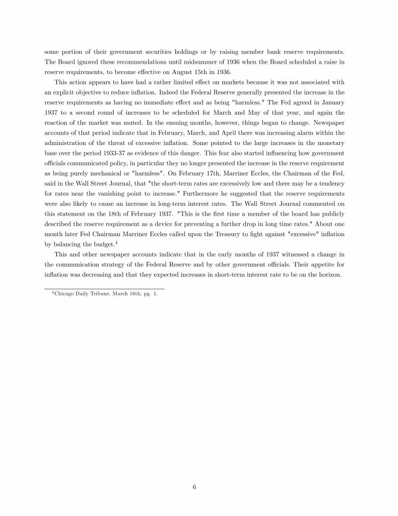
Table 1: The Mistake of 1937: Anti-inflationary Communcation1. July 14, 1936 The Federal Reserve announces the firs t reserve requirement increase
which will become effective on the 15th of August.
2. January 30, 1937 The Federal Reserve announces the second and third reserve requirement increaseswhich will become effective the 1s t of March and 1st of May.
3. February 18, 1937 Marriner Ecclees , Chairman of the Board of Governors , in Senate hearings: "The short term rates are excessively low and there may be a tendency for rates near the vanishing point to increase." --- Wall Street Journal, February 19, 1937, pg. 1.
4. March 15, 1937 Marriner Ecclees , Chairman of the Board of Governors , gives a s tatement: "The upward spiral of wages and prices into inflationary levels can be as disastrous as the downwards spiral of deflation." --- Chicago Daily Tribune, March 16, pg. 1.
5. March 17, 1937 Commerce Secretary Daniel C. Roper and Secretary of Agriculture Henry A. Wallace hold press conferences: Both Secretaries warn against excessive inflation.--- Wall Street Journal, March 18, 1937, pg. 8.
6. March 24, 1937 Marriner Eccles , Charimain of the Board of Governors , on inflation: "Chairmain Eccles outlines five s teps to avert 'dangerous inflation' in Forbes Magazine which are (i) resever requirement "to eliminate excess reserves", fiscal policy, (ii) fiscal policy that balances the budget (iii) reduction in the gold price of the dollar, (iv) increase in the labor share of national income (v) antitrus t legis lation." --- The Christian Science Monitor, March 25, 1937.
7. April 2, 1937 Franklin Delano Roosevel holds a press conference: "I am concerned -- we are all concerned -- over the price rise in certain materials ."
8. August 3, 1937 Franklin Delano Roosvelt views on price level targeting revealed: Senator Elmer Thomaspublished a letter from Franklin Delano Rosevelt to him rejecting his proposal that the Federal Reserve should formally target the 1926 price level.--- Wall Street Journal, August 4, 1937, pg. 6.
Table 1 list several other announcements by key administration officials dating back to the recommen-
dation of the Advisory Board in November 1935. The table shows several signals about the commitment
to lower inflation in the early months of 1937, but that was the period during which most of the key policy
announcements were made. These announcements and their effect on public beliefs form the core of the
paper. We argue that these communications are the mistake of 1937. The mistake is exemplified in FDR’s
press conference comments on April 2, 1937: "I am concerned — we are all concerned — over the price rise
in certain materials." On the day of this announcement the stockmarket fell by 6 percent. The next day
the Wall Street Journal reported as follows:
There was a feeling among some bankers that the President’s remarks bore a relation to the
recent statement of M. Eccles, Chairman of the Board of Governors of the Federal Reserve
System, advocating prompt balancing of the budget as the only means of averting monetary in-
flation and the other recent statements of government officials warning of the threat of inflation.
All of these remarks, it was said, indicated a change in the trend of the government’s recovery
measures away from the emphasis which has been placed upon stimulation of industrial activity
and the recovery of prices.
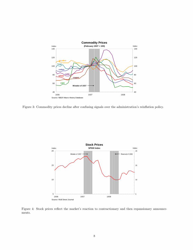
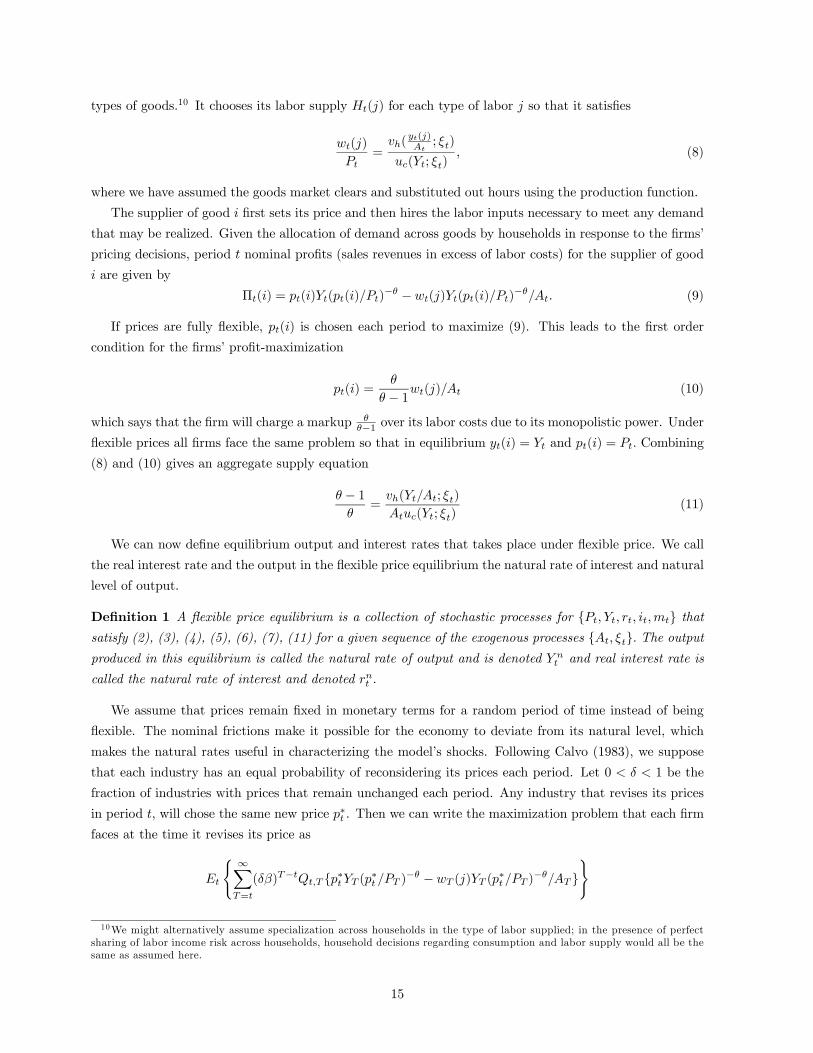
Figure 3 shows the response of leading commodity prices in a one year window surrounding several of
the statements listed in table 1. The period of the key announcements, i.e. the one made from February
to May, is marked by a shaded region. The monthly price indices are reindexed to 100 in February 1937
to allow better compare their relative paths5. Since commodity prices are determined on spot markets
5These data are monthly price indices of various commodities are archived in the NBER Macrohistory database.
7
40
60
80
100
120
140
1936 1937 193840
60
80
100
120
140
Source: NBER Macro History Database
wheat
cotton
corn
cattle
hogs
copper
gasoline
Commodity Prices(February 1937 = 100)Index Index
Mistake of 1937
Figure 3: Commodity prices decline after confusing signals over the administration’s reinflation policy.
5
10
15
20
1936 1937 19385
10
15
20
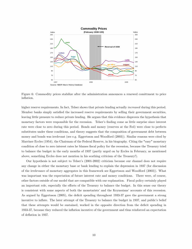
Source: Wall Street Journal
Index Index
Stock PricesSP500 Index
Mistake of 1937 Reversal of 1938
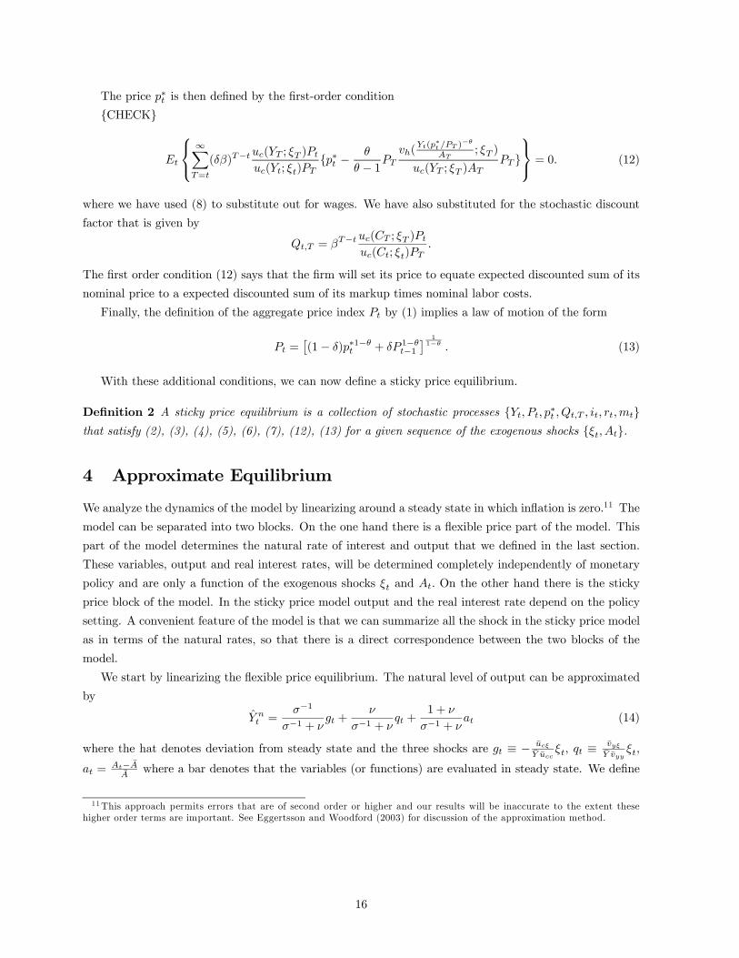
Figure 4: Stock prices reflect the market’s reaction to contractionary and then expansionary announce-ments.
8

0
1
2
3
4
5
6
1929 1931 1933 1935 1937 1939 19410
1
2
3
4
5
6
Source: Bureau of Labor Statistics, Cechetti
Short Term Interest RateEstimated Constant Maturity YieldPercent Percent
Figure 5: Interest rates remain close to zero througout the entire period.
one would expect their prices to respond more strongly than other goods’ to news about changes in future
policy. All of these commodity prices show a strong change in their upward trend in the early part of 1937
towards deflation. The price of corn, for example, lost more than half its value in the six month period
following FDR’s April announcement. Figure 4 show that the stock market also started a strong downward
trend—losing almost half its value in only six months.
The near-zero interest rates throughout the period have sometimes led to the conclusion that monetary
policy was not contractionary (see e.g. Telser (2001-2002)) and that monetary conditions were in fact
"easy". We find that more than short-term interest rates, changing expectations about future interest
rates, and how in these months they depended on inflation and output, are important to explain the
economic collapse. Figure 5 shows the evolution of the short-term interest rate in 1930-1941 as measured
by estimated yields in 3-month Treasuries. From late 1932 onwards the short-term interest rate remained
close to zero. In the spring of 1937 it rose only slightly and then fell again. These persistently low rates
stand at odds with the collapse in output and inflation in 1937. In the model we present in the next
sections, however, an increase in the current short-term interest rate is not required for contractionary
monetary policy. All that is needed is an expectation of future policy change. Indeed, our model assumes
that there is no change in the short-term interest rate during this period. Even with this assumption the
model delivers a large contractionary outcome only due to a change in expectations about future policy.
A leading hypothesis of the contraction of 1937-38 is suggested by Friedman and Schwartz (1963).
These authors argue that the increase in the reserve requirements in August 1936 and March and May
1937 were responsible for the contraction. This hypothesis has been criticized on several grounds. The
most plausible criticism of their theory is obtained by empirically evaluating their suggested transmission
mechanism during this period, which L.G. Telser analyzes in his (2001-2002) article "Higher member bank
reserve ratios in 1936 and 1937 did not cause the relapse into depression." The Friedman and Schwartz
hypothesis, according to Telser, implies that member bank lending should have declined in response to the
9
50
70
90
110
130
150
170
190
210
230
250
1937 1938 193950
70
90
110
130
150
170
190
210
230
250
Source: NBER Macro History Database
wheat
cotton
corn
cattle
hogs
coppergasoline
Commodity Prices(February 1938=100)Index Index
Reversal of 1938
Figure 6: Commodity prices stabilize after the administration announces a renewed comittment to priceinflation.
higher reserve requirements. In fact, Telser shows that private lending actually increased during this period.
Member banks simply satisfied the increased reserve requirements by selling their government securities,
leaving little pressure to reduce private lending. He argues that this evidence disproves the hypothesis that
monetary factors were responsible for the recession. Telser’s finding come as little surprise since interest
rate were close to zero during this period. Bonds and money (reserves at the Fed) were close to perfects
substitutes under these conditions, and theory suggests that the composition of government debt between
money and bonds was irrelevant (see e.g. Eggertsson and Woodford (2003)). Similar reasons were cited by
Marriner Eccles (1954), the Chairman of the Federal Reserve, in his biography. Citing the "easy" monetary
condition of close to zero interest rates he blames fiscal policy for the recession, because the Treasury tried
to balance the budget in the early months of 1937 (partly urged on by Eccles in February, as mentioned
above, something Eccles does not mention in his scathing criticism of the Treasury!).
Our hypothesis is not subject to Telser’s (2001-2002) criticism because our channel does not require
any change in either the monetary base or bank lending to explain the depression in 1937 (for discussion
of the irrelevance of monetary aggregates in this framework see Eggertsson and Woodford (2003)). What
was important was the expectation of future interest rate and money conditions. There were, of course,
other factors outside of our model that are compatible with our explanation. Fiscal policy certainly played
an important role, especially the efforts of the Treasury to balance the budget. In this sense our theory
is consistent with some aspects of both the monetarists’ and the Keynesians’ accounts of this recession.
As argued by Eggertsson (2005), the deficit spending throughout 1933-37 gave the government a strong
incentive to inflate. The later attempt of the Treasury to balance the budget in 1937, and public’s belief
that these attempts would be sustained, worked in the opposite direction from the deficit spending in
1933-37, because they reduced the inflation incentive of the government and thus reinforced an expectation
of deflation in 1937.
10
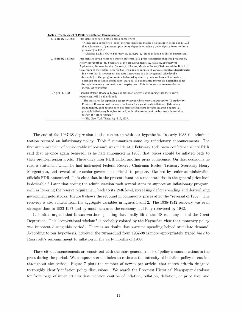
Table 2. The Reversal of 1938: Pro-inflation Communcation1. February 15, 1938 President Roosevelt holds a press conference:
"At his press conference today, the President said that he believes now, as he did in 1933, that achivement of permanent prosperity depends on raising general price levels to those prevailing in 1926." --- Chicago Daily Tribute, February 16, 1938, pg. 1, "Hope Inflation W ill Halt Depress ion."
2. February 18, 1938 President Rosevelt releases a written s tatement at a press conference that was prepared byHenry Morgenthau, Jr., Secretary of the Treasury; Henry A. Wallace, Secretary of Agriculture; Frances Perkins , Secretary of Labor; Marriner Eccles , Chairman of the Board ofGovernors of the Federal Reserve System, and economists of various executive departments: It is clear that in the present s ituation a moderate rise in the general price level is desirable [....] Our program seeks a balanced system of prices such as will promote a balanced expansion in production. Our goal is a constantly increas ing national income through increas ing production and employment. This is the way to increase the real income of consumers .
3. April 14, 1938 Franklin Delano Roosevelt, gives addresses Congress announcing that the reserve requirement will be abandoned: "The measures for expanding excess reserves which were announced on Thursday by President Roosevel will re-create the bases for a great credit inflation [..].Monetary management, after having been directed for some time towards guarding agains t a possible inflationary boo, has turned, under the pressure of the business depression, toward the other extreme." --- The New York Times, April 17, 1937.
The end of the 1937-38 depression is also consistent with our hypothesis. In early 1938 the adminis-
tration restored an inflationary policy. Table 2 summarizes some key reflationary announcements. The
first announcement of considerable importance was made at a February 15th press conference where FDR
said that he once again believed, as he had announced in 1933, that prices should be inflated back to
their pre-Depression levels. Three days later FDR called another press conference. On that occasions he
read a statement which he had instructed Federal Reserve Chairman Eccles, Treasury Secretary Henry
Morgenthau, and several other senior government officials to prepare. Flanked by senior administration
officials FDR announced, "it is clear that in the present situation a moderate rise in the general price level
is desirable." Later that spring the administration took several steps to support an inflationary program,
such as lowering the reserve requirement back to its 1936 level, increasing deficit spending and desterilizing
government gold stocks. Figure 6 shows the rebound in commodity prices after the "reversal of 1938." The
recovery is also evident from the aggregate variables in figures 1 and 2. The 1938-1942 recovery was even
stronger than in 1933-1937 and by most measures the economy had fully recovered by 1942.
It is often argued that it was wartime spending that finally lifted the US economy out of the Great
Depression. This "conventional wisdom" is probably colored by the Keynesian view that monetary policy
was impotent during this period. There is no doubt that wartime spending helped stimulate demand.
According to our hypothesis, however, the turnaround from 1937-38 is more appropriately traced back to
Roosevelt’s recommitment to inflation in the early months of 1938.
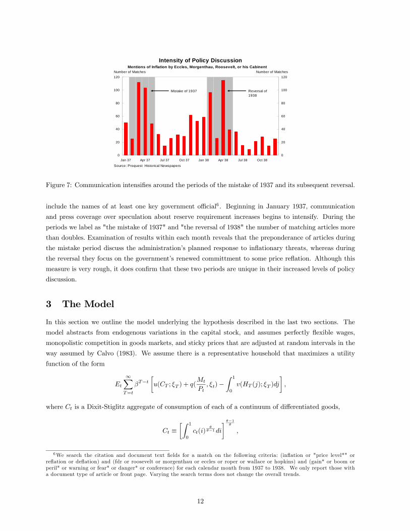
These cited announcements are consistent with the more general trends of policy communications in the
press during the period. We compute a crude index to estimate the intensity of inflation policy discussion
throughout the period. Figure 7 plots the number of newspaper articles that match criteria designed
to roughly identify inflation policy discussions. We search the Proquest Historical Newspaper database
for front page of inner articles that mention caution of inflation, reflation, deflation, or price level and
11
0
20
40
60
80
100
120
Jan 37 Apr 37 Jul 37 Oct 37 Jan 38 Apr 38 Jul 38 Oct 380
20
40
60
80
100
120
Source: Proquest Historical Newspapers
Intensity of Policy DiscussionMentions of Inflation by Eccles, Morgenthau, Roosevelt, or his Cabinent
Number of Matches Number of Matches
Mistake of 1937 Reversal of 1938
Figure 7: Communication intensifies around the periods of the mistake of 1937 and its subsequent reversal.
include the names of at least one key government official6 . Beginning in January 1937, communication
and press coverage over speculation about reserve requirement increases begins to intensify. During the
periods we label as "the mistake of 1937" and "the reversal of 1938" the number of matching articles more
than doubles. Examination of results within each month reveals that the preponderance of articles during
the mistake period discuss the administration’s planned response to inflationary threats, whereas during
the reversal they focus on the government’s renewed committment to some price reflation. Although this
measure is very rough, it does confirm that these two periods are unique in their increased levels of policy
discussion.
3 The Model
In this section we outline the model underlying the hypothesis described in the last two sections. The
model abstracts from endogenous variations in the capital stock, and assumes perfectly flexible wages,
monopolistic competition in goods markets, and sticky prices that are adjusted at random intervals in the
way assumed by Calvo (1983). We assume there is a representative household that maximizes a utility
function of the form
Et
∞XT=t
βT−t∙u(CT ; ξT ) + q(
Mt
Pt, ξt)−
Z 1
0
v(HT (j); ξT )dj
¸,
where Ct is a Dixit-Stiglitz aggregate of consumption of each of a continuum of differentiated goods,
Ct ≡∙Z 1
0
ct(i)θ
θ−1 di
¸ θ−1θ
,
6We search the citation and document text fields for a match on the following criteria: (inflation or "price level*" orreflation or deflation) and (fdr or roosevelt or morgenthau or eccles or roper or wallace or hopkins) and (gain* or boom orperil* or warning or fear* or danger* or conference) for each calendar month from 1937 to 1938. We only report those witha document type of article or front page. Varying the search terms does not change the overall trends.
12
with an elasticity of substitution equal to θ > 1. Ht(j) is the quantity of labor supplied to industry j,
where each industry employs a specific type of labor that demands wages wt(j). Pt is the Dixit-Stiglitz
price index,
Pt ≡∙Z 1
0
pt(i)1−θdi
¸ 11−θ
(1)
where pt(i) is the price of good i.
For each value of the disturbances ξt, u(·; ξt) is concave function that is increasing in consumption.Similarly, for each value of ξt, q(·; ξt) is increasing up to a satiation point at some finite level of realmoney balances as in Friedman (1969)7. v(·; ξt) is an increasing convex function. The vector of exogenousdisturbances ξt may contain several elements, so we make no assumption about any correlation of the
exogenous shifts in the functions u, q and v.
For simplicity we assume complete financial markets and no limits on borrowing against future income.
As a consequence, the household faces an intertemporal budget constraint of the form
Et
∞XT=t
Qt,TPTCT ≤Wt +Et
∞XT=t
Qt,T
∙Z 1
0
ΠT (i)di+
Z 1
0
wT (j)HT (j)dj − TT
¸
looking forward from any period t. Here Qt,T is the stochastic discount factor by which the financial
markets value random nominal income at date T in monetary units at date t, it is the riskless nominal
interest rate on one-period obligations purchased in period t, Wt is the nominal value of the household’s
financial wealth at the beginning of period t, Πt(i) represents the nominal profits (revenues in excess of
the wage bill) in period t of the supplier of good i, wt(j) is the nominal wage earned by labor of type j in
period t, and Tt represents the net nominal tax liabilities of each household in period t.
Optimizing household behavior then implies the following necessary conditions for a rational-expectations
equilibrium. Optimal timing of household expenditure requires that aggregate demand Yt for the composite
good8 satisfy an Euler equation of the form
uc(Yt, ξt) = βEt
∙uc(Yt+1, ξt+1)(1 + it)
PtPt+1
¸. (2)
Optimal money holding implies thatqm(mt, ξt)
uc(Yt, ξt)=
it1 + it
, (3)
where mt ≡ Mt
Pt. This equation defines money demand. Utility is weakly increasing in real money balances,
but it does not increase beyond finite level of money balances. The left hand side of this equation is
therefore weakly positive. Thus there is a zero bound on the short-term nominal interest rate given by
it ≥ 0 (4)
7The idea is that real money balances enter the utility because they facilitate transactions. At some finite level of realmoney balances, e.g. when the representative household holds enough cash to pay for all consumption purchases in thatperiod, holding more real money balances will not facilitate transaction any further and thereby add nothing to utility. Thisis at the “satiation” point of real money balances. We assume that there is no storage cost of holding money so increasingmoney holding can never reduce utility directly through u(.). A satiation level in real money balances is also implied byseveral cash-in-advance models such as Lucas and Stokey (1987) or Woodford (1998).
8For simplicity, we abstract from government purchases of goods.
13
The intuition for this bound is simple. Since the model has no storage cost of holding money and it can be
held as an asset. The result follows the return on bonds must be at least as good as that on money, and
thus that it cannot be a negative number. No one would lend 100 dollar unless she expects to receive at least
100 dollars back! Household optimization similarly requires that the paths of aggregate real expenditure
and the price index satisfy the conditions
∞XT=t
βTEtuc(YT , ξT )YT <∞, (5)
limT→∞
βTEt[uc(YT , ξT )WT /PT ] = 0 (6)
looking forward from any period t. Wt measures the total nominal value of government liabilities, which
are held by the household, and are the sum of Bt and Mt. Condition (5) is required for the existence of
a well-defined intertemporal budget constraint, under the assumption that there are no limitations on the
household’s ability to borrow against future income, while the transversality condition (6) must hold if the
household exhausts its intertemporal budget constraint. Conditions (2) — (6) also suffice to imply that the
representative household chooses optimal consumption and portfolio plans (including its planned holdings
of money balances) given its income expectations and the prices (including financial asset prices) that it
faces, while making choices that are consistent with clearing financial markets. For simplicity we assume
throughout that the government issues no debt so that 6 is always satisfied.
We also find it convenient for our exposition to define the price for a one period real bond. This bond
promises its buyer to pay one unit of a consumption good tomorrow, with certainty, for a price of 1 + rt.
This number is the short term real interest rate. While this price is well defined, no such bonds will
be traded in equilibrium, because we assume a representative household. It follows from the household
maximization problem that the real interest rate satisfies the arbitrage equation
uc(Yt, ξt) = (1 + rt)βEtuc(Yt+1, ξt+1) (7)
Each differentiated good i is supplied by a single monopolistically competitive producer. There are
assumed to be many goods in each of an infinite number of “industries”; the goods in each industry j are
produced using a type of labor that is specific to that industry and also change their prices at the same
time. Each good is produced in accordance with a common production function9
yt(i) = Atht(i),
where At is an exogenous productivity factor common to all industries, and ht(i) is the industry-specific
labor hired by firm i. The representative household supplies all types of labor as well as consuming all
9There is no loss of generality in assuming a linear production function because we allow for arbitary curvature in thedisutility of working.
14
types of goods.10 It chooses its labor supply Ht(j) for each type of labor j so that it satisfies
wt(j)
Pt=
vh(yt(j)At; ξt)
uc(Yt; ξt), (8)
where we have assumed the goods market clears and substituted out hours using the production function.
The supplier of good i first sets its price and then hires the labor inputs necessary to meet any demand
that may be realized. Given the allocation of demand across goods by households in response to the firms’
pricing decisions, period t nominal profits (sales revenues in excess of labor costs) for the supplier of good
i are given by
Πt(i) = pt(i)Yt(pt(i)/Pt)−θ − wt(j)Yt(pt(i)/Pt)
−θ/At. (9)
If prices are fully flexible, pt(i) is chosen each period to maximize (9). This leads to the first order
condition for the firms’ profit-maximization
pt(i) =θ
θ − 1wt(j)/At (10)
which says that the firm will charge a markup θθ−1 over its labor costs due to its monopolistic power. Under
flexible prices all firms face the same problem so that in equilibrium yt(i) = Yt and pt(i) = Pt. Combining
(8) and (10) gives an aggregate supply equation
θ − 1θ
=vh(Yt/At; ξt)
Atuc(Yt; ξt)(11)
We can now define equilibrium output and interest rates that takes place under flexible price. We call
the real interest rate and the output in the flexible price equilibrium the natural rate of interest and natural
level of output.
Definition 1 A flexible price equilibrium is a collection of stochastic processes for {Pt, Yt, rt, it,mt} thatsatisfy (2), (3), (4), (5), (6), (7), (11) for a given sequence of the exogenous processes {At, ξt}. The outputproduced in this equilibrium is called the natural rate of output and is denoted Y n
t and real interest rate is
called the natural rate of interest and denoted rnt .
We assume that prices remain fixed in monetary terms for a random period of time instead of being
flexible. The nominal frictions make it possible for the economy to deviate from its natural level, which
makes the natural rates useful in characterizing the model’s shocks. Following Calvo (1983), we suppose
that each industry has an equal probability of reconsidering its prices each period. Let 0 < δ < 1 be the
fraction of industries with prices that remain unchanged each period. Any industry that revises its prices
in period t, will chose the same new price p∗t . Then we can write the maximization problem that each firm
faces at the time it revises its price as
Et
( ∞XT=t
(δβ)T−tQt,T {p∗tYT (p∗t /PT )−θ − wT (j)YT (p∗t /PT )
−θ/AT })
10We might alternatively assume specialization across households in the type of labor supplied; in the presence of perfectsharing of labor income risk across households, household decisions regarding consumption and labor supply would all be thesame as assumed here.
15
The price p∗t is then defined by the first-order condition
{CHECK}
Et
⎧⎨⎩∞XT=t
(δβ)T−tuc(YT ; ξT )Ptuc(Yt; ξt)PT
{p∗t −θ
θ − 1PTvh(
Yt(p∗t /PT )
−θ
AT; ξT )
uc(YT ; ξT )ATPT }
⎫⎬⎭ = 0. (12)
where we have used (8) to substitute out for wages. We have also substituted for the stochastic discount
factor that is given by
Qt,T = βT−tuc(CT ; ξT )Ptuc(Ct; ξt)PT
.
The first order condition (12) says that the firm will set its price to equate expected discounted sum of its
nominal price to a expected discounted sum of its markup times nominal labor costs.
Finally, the definition of the aggregate price index Pt by (1) implies a law of motion of the form
Pt =£(1− δ)p∗1−θt + δP 1−θt−1
¤ 11−θ . (13)
With these additional conditions, we can now define a sticky price equilibrium.
Definition 2 A sticky price equilibrium is a collection of stochastic processes {Yt, Pt, p∗t , Qt,T , it, rt,mt}that satisfy (2), (3), (4), (5), (6), (7), (12), (13) for a given sequence of the exogenous shocks {ξt, At}.
4 Approximate Equilibrium
We analyze the dynamics of the model by linearizing around a steady state in which inflation is zero.11 The
model can be separated into two blocks. On the one hand there is a flexible price part of the model. This
part of the model determines the natural rate of interest and output that we defined in the last section.
These variables, output and real interest rates, will be determined completely independently of monetary
policy and are only a function of the exogenous shocks ξt and At. On the other hand there is the sticky
price block of the model. In the sticky price model output and the real interest rate depend on the policy
setting. A convenient feature of the model is that we can summarize all the shock in the sticky price model
as in terms of the natural rates, so that there is a direct correspondence between the two blocks of the
model.
We start by linearizing the flexible price equilibrium. The natural level of output can be approximated
by
Y nt =
σ−1
σ−1 + νgt +
ν
σ−1 + νqt +
1 + ν
σ−1 + νat (14)
where the hat denotes deviation from steady state and the three shocks are gt ≡ − ucξY ucc
ξt, qt ≡vyξY vyy
ξt,
at =At−AA
where a bar denotes that the variables (or functions) are evaluated in steady state. We define
11This approach permits errors that are of second order or higher and our results will be inaccurate to the extent thesehigher order terms are important. See Eggertsson and Woodford (2003) for discussion of the approximation method.
16
the parameters σ ≡ −uccYuc
and ν ≡ vhvhhh
. The natural rate of interest can similarly be linearized as
rnt =1− β
β+
σ−1β−1
σ−1 + υ(gt −Etgt+1) +
υβ−1
σ−1 + υ(qt −Etqt+1) +
(1 + υ)β−1
σ−1 + υ(at −Etat+1) (15)
We now turn to the sticky price equilibrium. As mentioned above a convenient feature of the model is
that the all the shocks can be summarized in terms of the flexible price equilibrium variables Y nt and rnt
in addition to a money demand shock.
We can express the consumption Euler equation (2) as12
Yt − Y nt = EtYt+1 −EtY
nt+1 − σ(it −Etπt+1 − rnt ) (16)
This equation says that current demand depends on expectations of future output — since spending depends
on expected future income — and the real interest rate which is the difference between the nominal interest
rate and expected future inflation — because lower real interest rate make spending today relatively cheaper
to future spending. This equation can be forwarded to yield
Yt − Y nt = EtYT+1 −EtY
nT+1 − σ
TXs=t
(is −Etπs+1 − rns )
which illustrates that the demand does not only depend on the current interest rate but the entire ex-
pected path for future interest rates and expected inflation. Because long-term interest rates depend on
expectations about current and future short rates the equation above can also be interpreted as saying that
demand depends on long-term interest rates.
The Euler equation (12) of the firms’ maximization problem, together with the price dynamics (13),
can be approximated to yield
πt = κ(Yt − Y nt ) + βEtπt+1 (17)
where κ ≡ (1−δ)(1−δβ)δ
ν+σ−1
1+νθ > 0. This equation implies that inflation can increase output because not all
firms will reset their prices instantaneously, leading to a lower real wages than in a flexible price equilibrium,
thus supporting an output expansion.
Finally the money demand equation along with the zero bound can be summarized as
mt ≥ ηiit + ηyYt + t (18)
it ≥ 0 (19)
it(mt − ηiit − ηyYt − t) = 0 (20)
where ηi < 0 and ηy > 0, and t ≡ −ηi 1−ββ +ucξ−qmξ
qmmξt and the last condition is a complementary slackness
condition that says that the money demand equation must hold with equality if the zero bound is slack
12 In this approximated equation the variable it refers to interest rate defined before times β−1 and is not defined in termsof deviation from stead state like some of the other variables. I do this to simplify notation, i.e. so that I can express thezero bound as the constraint that it cannot be less than zero.
17
(and similarly that the zero bound must be binding if the money demand equality is slack). Because the
shocks in the sticky price equilibrium are now completely summarized by the stochastic processes of rntand Y n
t and t we can define an approximate sticky price equilibrium as follows.
Definition 3 An approximate sticky price equilibrium is a collection of stochastic professes for {Yt, πt,mt, it}that satisfy (16)-(20) for a given sequence for the exogenous shocks {Y n
t , rnt , t}.
5 Policy Regimes, Structural Shocks and Communications
To model the effect of communications at zero interest rates we need to take a stance on two things, (i)
the shock processes that drive the dynamics of the model and (ii) the policy regimes.
Recall from last section that all the shocks of the model can be summarized by the natural rates.13
Following Eggertsson and Woodford (2003), we assume the most simple process for the exogenous shocks
that give rise to zero interest rates.
A1: The Great Depression structural shocks rnt = rnL < 0 at date t = 0. It returns back to steady
state rnH with probability α in each period. Furthermore, Y nt = 0 ∀ t. The stochastic date the shock
returns back to steady state is denoted τ . To ensure a bounded solution the probability α is such that
α(1− β(1− α))− σκ(1− α) > 0
We model communication as corresponding to signals about the likelihood of a regime change. In the
next two subsection we propose two policy regimes to which these signals apply.
5.1 The Deflationary Regime
We first study equilibrium under the assumption that the central bank targets a zero inflation target
whenever possible. This is what we call Policy Regime 1 or "the deflationary regime". Zero inflation
implies by (17) a zero deviation of output when there are no shocks so that assuming A1 then
πt = Yt = 0 if t ≥ τ (21)
which implies by (16) that
it = rnt if t ≥ τ . (22)
A zero inflation target cannot be achieved in periods t < τ , however, because this would imply nega-
tive nominal interest rates. We assume that in this case the central bank allows for maximum policy
accommodation and sets the interest rate at zero, i.e.
it = 0 for 0 < t < τ (23)
An equilibrium under Policy Regime 1 is now defined as
Definition 4 The Deflationary Policy Regime. Equilibrium under Policy Regime 1 and assuming A1 is
an approximate equilibrium defined in Definition 3 that satisfies equations (21)-(23).
13With the exception of t but we do not need to take a stance on this shock.
18
−5 0 5 10 15 20−30
−20
−10
0
10inflation
−5 0 5 10 15 20−40
−20
0
output
−5 0 5 10 15 20−2
0
2
4
interest rates
Figure 8: Output contraction at zero interest rates.
To solve for inflation and output we can solve equation (17) and (16) by using (21)-(23). The value
for πt and Yt that solve these equation in period t < τ are the numbers πd and Y d (where D stands for
"deflationary regime") that solve the two equations
πd = κY d + β(1− α)πd
Y d = (1− α)Y d + σ(1− α)πd + σrnL
yielding
Y d =1− β(1− α)
α(1− β(1− α))− σκ(1− α)σrnL < 0 (24)
πd =1
γ(1− β(1− α))− σκ(1− α)κσrnL < 0 (25)
Table 3parameters calibrated values
σ 0.5
ν 2
β 0.99
θ 10
κ 0.02
α 0.1
rnL -0.04
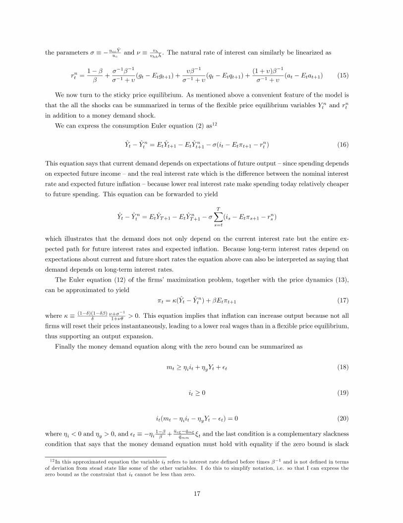
Figure 8 shows the output contraction and deflation under A1 that is predicted by the model. The
parameters assumed are shown in Table 3 and are taken directly from Eggertsson and Woodford (2003) and
Eggertsson (2006a). The parameter σ is the intertemporal elasticity of substitution (so that the coefficient
of relative risk aversion is 2, which is in line with micro evidence), ν is the inverse of Frisch labor supply
19
(implying a Frisch elasticity of 0.5, which is also in line with micro evidence), β is calibrated to match a
steady state real interest rate of 4% per year, θ corresponds to a markup of 10 percent. The parameter
κ is from the estimate by Rotemberg and Woodford (1997). The the probability of the shock reverting in
the next period α is calibrated at 10 percent, which implies an expected duration of 10 periods.
In the figure it is assumed that the natural rate of interest is −4 percent in the rnL state to match theoutput contraction during the Great Depression. The figure shows the case in which the natural rate of
interest returns to steady state in period τ = 10 (which is the expected duration of the shock). The model
indicates an output collapse of 30% under this calibration and the contraction lasts as long as the duration
of the shock. The contraction at any time t is created by a combination of the deflationary shock in period
t < τ — but more importantly — the expectation that there will be deflation and output contraction in
future periods periods t+ j < τ for j > 0. The deflation in period t+ j in turn depends on expectations
of deflation and output contraction in periods t+ j + i < τ for i > 0. This creates vicious feedback effects
that will not even converge unless the restriction on α in A1 is satisfied. The overall effect is an output
collapse as shown in figure 8 for a relatively small shock to the natural rate of interest.14 The duration of
the contraction can be several years in the model, or as long as the shocks last.
The large collapse in output and prices reflect the strong contractionary effects brought about by
nominal frictions One observes that the flexible price output is constant throughout this period so that it
is only the interplay between the intertemporal shock rnL and nominal frictions that bring about the output
collapse.
5.2 The Reflationary Regime
We now consider the consequences of a reflationary regime, policy regime 2, in which the government
targets an inflation rate that is higher than zero, i.e. πt = π∗ > 0. Under A1 this implies that in policy
regime 2
πt = π∗ for t ≥ τ (26)
In addition we assume that the public believes with some probability γt that in the next period the
government will abandon policy regime 2 in favor of Policy Regime 1 for all future periods. The probability
γt is therefore the probability of moving to Policy Regime 1 in period t+1, conditional on being in Policy
Regime 2 in period t. We assume that this probability can change over time, for example, based on new
information about the administration’s policy intentions. It is natural to assume in the absence of any new
information about policy, the public beliefs will remain unchanged. This leads us to assume
Etγt+1 = γt, (27)
which says that conditional on all information in period t, the public expects to apply the same probability
to a regime change moving forward. One interpretation of the parameter γt is that it indicates the credibility
of the policy regime, because it is a measure of how probable the public thinks it is that the reflationary
14The sense in which the shock is "small" is that the real rate of interest (which is equal to rnt in the absence of an outputslack) has been of this order several times in US history, such as the 70s (see e.g. Summers (1991) for discussion). On thoseoccasions, however, there has been positive inflation so that negative real rate of interest has easily been accomodated.
20
policy regime will continue. If γ were deterministic then the expected duration of the regime would be 1γ
so that as γ approaches zero the regime is perfectly credible and the public believes the regime will last
forever, but when it is 1 the regime has no credibility, and the public expects it to be abandoned in the
next period.
A more interesting interpretation of γt has to do with its variations. Since this parameter is likely to
change in the light of new information about the policy intentions of the government, changing values of
γt can be interpreted as reflecting communications by the government about its policy objectives.
Under A1 the solution for output, denoted Y ∗t , at time t ≥ τ solves equation (17), i.e.
π∗ = κY ∗t + (1− γt)βπ∗ (28)
so that in the reflationary regime
Y ∗t = {1− β(1− γt)}κ−1π∗ (29)
and
it = rnt + (1− γt)π∗ at t ≥ τ
If rnt ≤ −π∗, however, the central bank cannot achieve the inflation target in period t < τ because
this may imply negative nominal interest rates. We assume that in this case the central bank allows for
maximum accommodation and sets the interest rate at zero, i.e.
it = 0 for 0 < t < τ (30)
An equilibrium under the reflationary regime, i.e. Policy Regime 2, can now be defined as follows:
Definition 5 Reflationary Regime. Equilibrium under Policy Regime 2, assuming A1, is an approximate
equilibrium defined in Definition 3 that satisfies equations (26)-(30).
To solve for equilibrium output and inflation in period t < τ we can use equation (17) and (16), using
(26)-(26), along with the solution (24) and (25). The value for πt and Yt that solve these equation in period
t < τ are the numbers πrt and Y rt where r stands for "reflationary regime" that solve the two equations.
πrt = κY rt + βEr
t πt+1 (31)
Y rt = Er
t Yt+1 + σErt πt+1 + σrnL (32)
The expectations are formed conditional on information at time t which takes into account that the current
regime is reflationary. We can express these expectations as
Ert πt+1 = (1− α)(1− γt)Et,rnt+1=r
nLπrt+1 + (1− α)γtπ
d + α(1− γt)π∗ (33)
were the first term denotes the contingency in which the shock rnt remains negative and the policy regime
is unchanged in period t+1. The expectation operator Et,rnt+1=rnLdenotes that expectations are taken with
respect to information at time t and conditional on that the natural rate of interest remaining negative in
21
period t+1. The superscript r an πrt+1 denotes the contingency that the regime is reflationary. The second
term is the contingency in which the shock remains negative but the regime changes to the deflationary
one (policy regime 1). The last term is the contingency in which the shock reverts to normal but the
the regime stays intact, in which case the government targets inflation of π∗. We can ignore the fourth
contingency that corresponds to the one in which the shock reverts to normal and the regime changes
because in this case the government targets zero inflation (and the term thus drops out). We can similarly
write the expectation for output as
Ert Yt+1 = (1− α)(1− γt)Et,t,rnt+1=r
nLY rt+1 + (1− α)γtY
d + α(1− γt)Y∗t (34)
A solution of the model is a sequence of numbers for Y rt and πrt that satisfy these four equations. We
look for a stationary solution of this system that is linear in the two state variables γt and rnt . In this case
πrt = Et,rnt+1=rnLπrt+1 and Y r
t = Et,t,rnt+1=rnLY rt+1 because of our assumed process for γt in equation (27).
Substituting (33) and (34) into (31) and (32) then πrt and Y rt solve
πrt = κY rt + β(1− α)(1− γt)π
rt + (1− α)γtπ
d + α(1− γt)π∗ (35)
Y rt = (1− α)(1− γt)Y
rt + (1− α)γtY
d + α(1− γt)Y∗t
+σ(1− α)(1− γt)πrt + σ(1− α)γtπ
d + σα(1− γt)π∗ + σrnL (36)
which yields
Y rt = A(γt)π
d +B(γt)π∗ (37)
+C(γt)Yd +D(γt)Y
∗t + F (γt)rL
where the value of each of the functions A,B,C,D,F are given in the footnote.15 All of these function only
depend on time through γt and are positive numbers. Given this solution one can write inflation as
πγt =κ
ΨtY rt +
β(1− α)γtΨt
πd +βα(1− γt)
Ψtπ∗ (38)
where 1 > Ψt = 1− β(1− α)(1− γt) > 0 and the the numbers πd and Y ∗t are given by (25) and (29).
As one would expect these equation are increasing in the inflation target π∗ and decreasing in the shock
rnL. The reason is that a higher inflation target increases expectation of future inflation and future output
15A(γt) =σ(1−α)γt+
σβ(1−α)2γt(1−γt)1−β(1−α)(1−γt)
1−(1−α)(1−γt)−κσ(1−α)(1−γt)1−β(1−α)(1−γt)
B(γt) =σα(1−γt)+
σβα(1−α)(1−γt)21−β(1−α)(1−γt)
1−(1−α)(1−γt)−κσ(1−α)(1−γt)1−β(1−α)(1−γt)
C(γt) =(1−α)γt
1−(1−α)(1−γt)−κσ(1−α)(1−γt)1−β(1−α)(1−γt)
D(γt) =α(1−γt)
1−(1−α)(1−γt)−κσ(1−α)(1−γt)1−β(1−α)(1−γt)
F (γt) =σ
1−(1−α)(1−γt)−κσ(1−α)(1−γt)1−β(1−α)(1−γt)
22

−5 0 5 10 15 20−30
−20
−10
0
10inflation
−5 0 5 10 15 20−30
−20
−10
0
10output
γ=0
γ=0.0063
γ=0.033
γ=1
Figure 9: Output and inflation are extreemely sensistive to small variations in the signal γt.
which in turn stimulates demand in each period t < τ. Thus a commitment to a future reflationary policy
mitigates the effects of the zero bound, as argued by Krugman (1998). In the forward looking model used
here these effect are very large, owing to the opposite effects of the vicious feedback effects described in the
last section.
Of even more interest to us is how the solution depends on the probability γt. Figure 9 shows the
solution in 37 and 38 under the assumption that the shock reverts at time τ = 10 and that under the
assumption that Policy Regime 2 is in effect throughout. It shows the solution under four possible values
of γt. When γt = 0 the inflation target is perfectly credible and when γt = 1 it has no credibility so
that the solution is identical to the one in figure 9. The intermediate cases are the ones of interest. When
γt = 0.033 there is 3.3 percent probability that the regime will be abandoned in the next period. This small
probability has a very large effect on output and prices, output is 20 percent lower than if the inflation
targeting regime is perfectly credible and there is about 15 percent deflation. Even when there is only 0.63
percent chance of a regime change the figure shows that the output collapse and effect on deflation are
substantial.
Table 4 transforms these probabilities into another probability measure, namely the probability that
the policy regime will be abandoned within two years, denoted ρt. Given our assumption that Etγt+1 = γt,
the probability ρt can be computed as
ρt = 1− (1− γt)8 (39)
We examine γt in this way because this variable has an appealing interpretation. The small number 0.0063,
for example, indicates that there is 4.3 percent chance that the regime will be abandoned within 2 years.
Table 4 shows the effect of various values of γt in terms of ρt on output for the values given in figure 9
Table 4
23
0 0.2 0.4 0.6 0.8 1−30
−25
−20
−15
−10
−5
0
5
γ
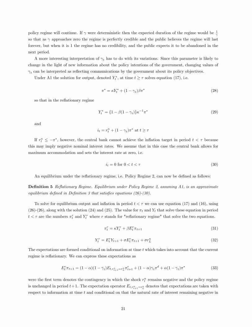
outputinflation
Figure 10: The response of output and inflation to changes in γt is non-linear and extremely sensitive atregions of high credibility.
γt ρt Yt when it = 0 Yt when it > 0
0 0 0.5 2.1
0.0063 0.043 -10.1 0.8
0.033 0.209 -20.4 0.5
1 1 -28.7 0These figures also demonstrate that while changes in expectations about the future monetary regimes
are extremely important at zero interest rates, they have a much smaller effect when interest rates are
positive. Thus while an increase in γt from 0% to 0.63% reduces output by -10.1% in the presence of large
deflationary shocks, the same type of communication only reduces output by 1.2 percent when the interest
rate is positive.
Figure 10 plots inflation and output as a function of γt. The figure shows the extreme sensitivity of
output and inflation to small variations in γt. This sensitivity is particularly strong at a "high level" of
credibility, i.e .when the public strongly believes in the reflationary policies.
The nonlinearity of the inflation and output in gamma may have some important policy implications.
It suggests — although this remains a bit speculative — that a preemptive tightening (or communication of
such a policy shift) has a large contractionary effect, while erring on the side of reflationary policy has a
much smaller effect. This may indicate that a prudent conservative approach to policy at a zero interest
rate favors erring on the side of inflation and accepting a rather slow response to inflationary pressure.
To put some more structure on this argument consider the consequences of sending a signal of "too
high inflation" in the sense of a signal of a inflation target above what is required to accommodate the -4%
negative natural rate of interest. Consider the effect of the same regime change as considered before but
now let Regime 1 now be characterized by a 8% inflation target instead of a 0 percent inflation target. In
this case an increase in γt is a signal of high inflation instead of too low inflation. If expectation of this
24
0 0.02 0.04 0.06 0.08 0.1−25
−20
−15
−10
−5
0
5output
low inflation signalhigh inflation signal
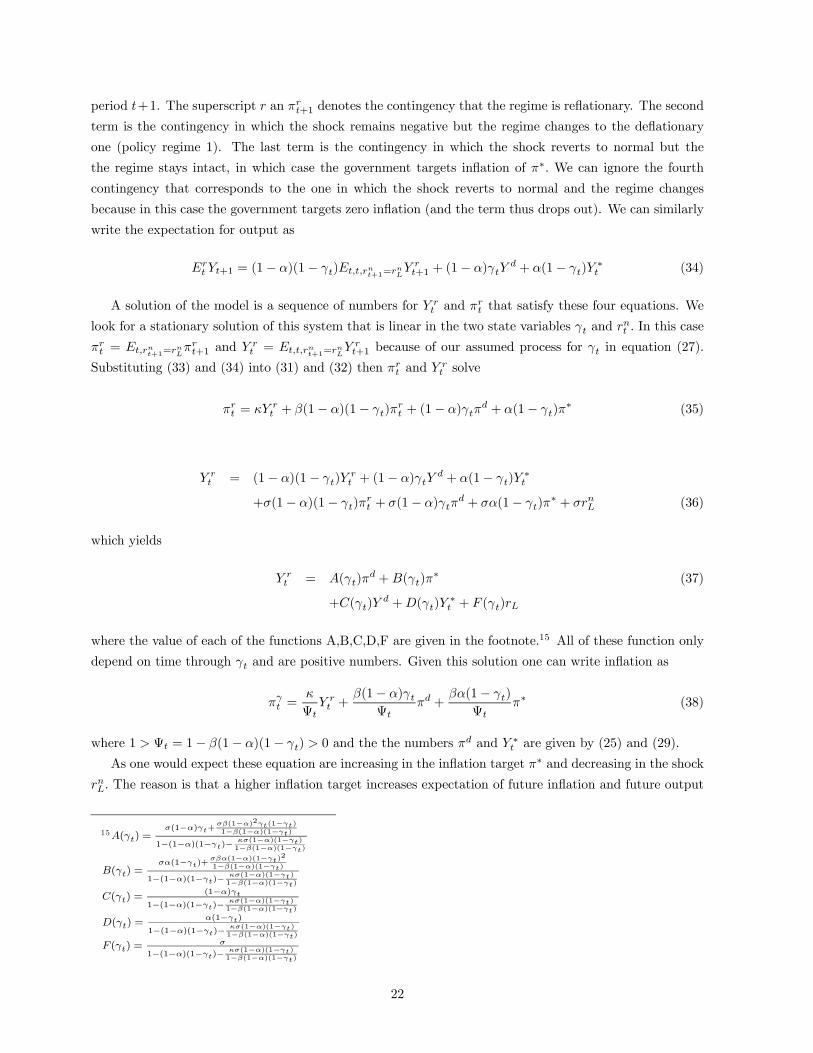
Figure 11: The nonlinearity of the zero bound indicates that output is much more sensitive to communcationthat indicate excessive tightening, than communication that imply too loose inflation policy.
inflationary regime are created then, conditional being in Policy Regime 2, πt = 4% and
it = rnt + (1− γt) ∗ 4%+ γt ∗ 8%
and output is given by the AS equation by
Yt = {1− β(1− γt)}κ−1 ∗ 4%− γtβκ−1 ∗ 8% (40)
Figure 11 shows that local to the fully credible inflation target of 4% output is extremely sensitive to
communication of a deflationary regime, while it responds by much less if the communication is about
excessively loose policy in the future.
6 The data on the Great Depression through the prism of the
model
The examples given in the last section are quite special in several respects, and they impose stark as-
sumptions for tractability. Keeping those limitations in mind, it is still of some interest to re-express the
data from the Great Depression through the prism of the model. We should state from the start that
we do not view this numerical exercise as a substitute for a full scale estimation of the model. Yet, we
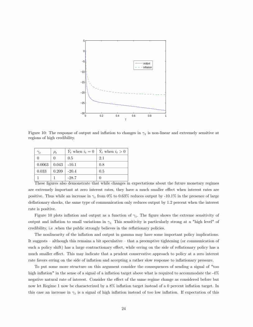
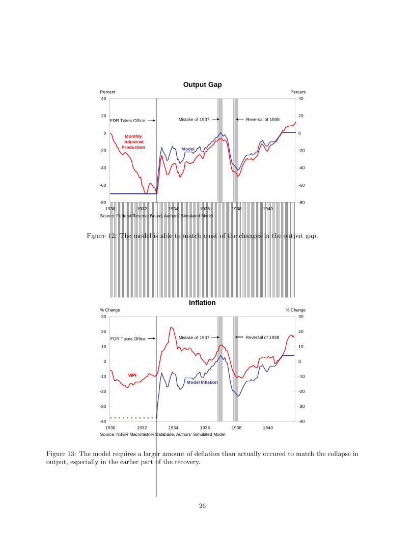
believe giving some closer connection to the data may be useful in developing the theory further. Figure 12
shows monthly data on industrial production from the Great Depression as a deviation from a linear trend
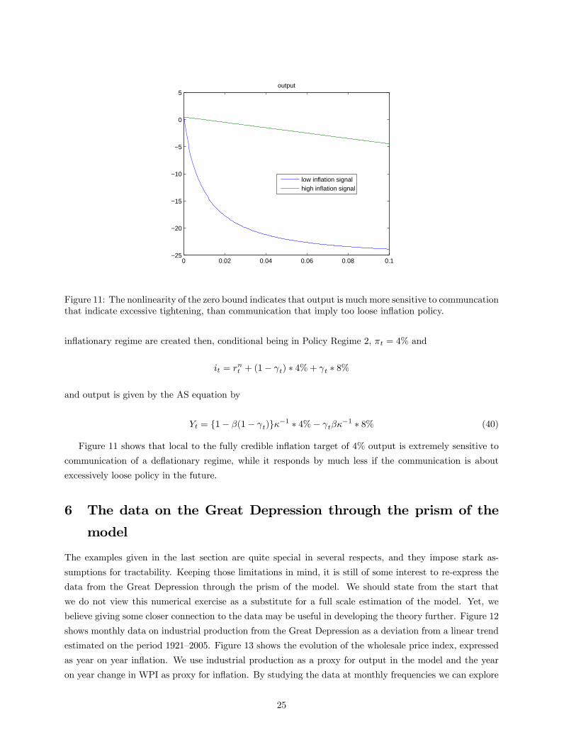
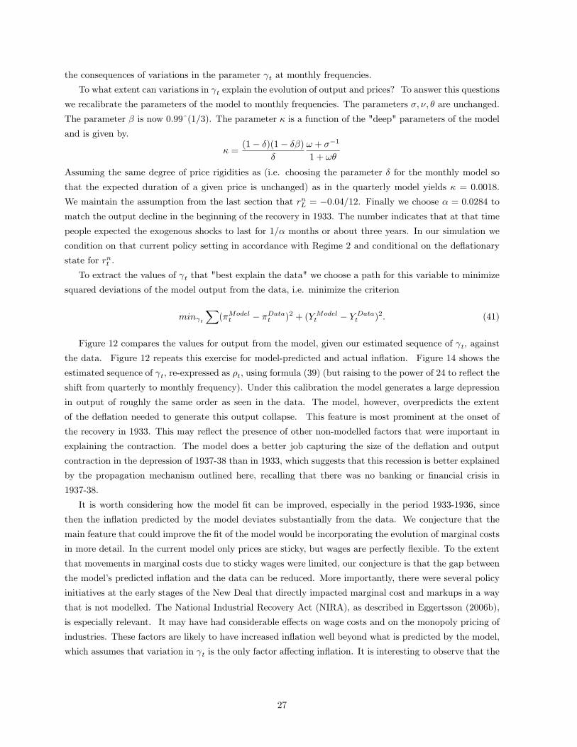
estimated on the period 1921—2005. Figure 13 shows the evolution of the wholesale price index, expressed
as year on year inflation. We use industrial production as a proxy for output in the model and the year
on year change in WPI as proxy for inflation. By studying the data at monthly frequencies we can explore
25
-80
-60
-40
-20
0
20
40
1930 1932 1934 1936 1938 1940-80
-60
-40
-20
0
20
40
Source: Federal Reserve Board, Authors' Simulated Model
Monthly Industrial
Production Model
Output GapPercent Percent
Mistake of 1937 Reversal of 1938FDR Takes Office
Figure 12: The model is able to match most of the changes in the output gap.
-40
-30
-20
-10
0
10
20
30
1930 1932 1934 1936 1938 1940-40
-30
-20
-10
0
10
20
30
Source: NBER Macrohistory Database, Authors' Simulated Model
WPI Model Inflation
Inflation% Change % Change
Mistake of 1937 Reversal of 1938FDR Takes Office
Figure 13: The model requires a larger amount of deflation than actually occured to match the collapse inoutput, especially in the earlier part of the recovery.
26
the consequences of variations in the parameter γt at monthly frequencies.
To what extent can variations in γt explain the evolution of output and prices? To answer this questions
we recalibrate the parameters of the model to monthly frequencies. The parameters σ, ν, θ are unchanged.
The parameter β is now 0.99ˆ(1/3). The parameter κ is a function of the "deep" parameters of the model
and is given by.
κ =(1− δ)(1− δβ)
δ
ω + σ−1
1 + ωθ
Assuming the same degree of price rigidities as (i.e. choosing the parameter δ for the monthly model so
that the expected duration of a given price is unchanged) as in the quarterly model yields κ = 0.0018.
We maintain the assumption from the last section that rnL = −0.04/12. Finally we choose α = 0.0284 tomatch the output decline in the beginning of the recovery in 1933. The number indicates that at that time
people expected the exogenous shocks to last for 1/α months or about three years. In our simulation we
condition on that current policy setting in accordance with Regime 2 and conditional on the deflationary
state for rnt .
To extract the values of γt that "best explain the data" we choose a path for this variable to minimize
squared deviations of the model output from the data, i.e. minimize the criterion
minγt
X(πModel
t − πDatat )2 + (YModel
t − Y Datat )2. (41)
Figure 12 compares the values for output from the model, given our estimated sequence of γt, against
the data. Figure 12 repeats this exercise for model-predicted and actual inflation. Figure 14 shows the
estimated sequence of γt, re-expressed as ρt, using formula (39) (but raising to the power of 24 to reflect the
shift from quarterly to monthly frequency). Under this calibration the model generates a large depression
in output of roughly the same order as seen in the data. The model, however, overpredicts the extent
of the deflation needed to generate this output collapse. This feature is most prominent at the onset of
the recovery in 1933. This may reflect the presence of other non-modelled factors that were important in
explaining the contraction. The model does a better job capturing the size of the deflation and output
contraction in the depression of 1937-38 than in 1933, which suggests that this recession is better explained
by the propagation mechanism outlined here, recalling that there was no banking or financial crisis in
1937-38.
It is worth considering how the model fit can be improved, especially in the period 1933-1936, since
then the inflation predicted by the model deviates substantially from the data. We conjecture that the
main feature that could improve the fit of the model would be incorporating the evolution of marginal costs
in more detail. In the current model only prices are sticky, but wages are perfectly flexible. To the extent
that movements in marginal costs due to sticky wages were limited, our conjecture is that the gap between
the model’s predicted inflation and the data can be reduced. More importantly, there were several policy
initiatives at the early stages of the New Deal that directly impacted marginal cost and markups in a way
that is not modelled. The National Industrial Recovery Act (NIRA), as described in Eggertsson (2006b),
is especially relevant. It may have had considerable effects on wage costs and on the monopoly pricing of
industries. These factors are likely to have increased inflation well beyond what is predicted by the model,
which assumes that variation in γt is the only factor affecting inflation. It is interesting to observe that the
27
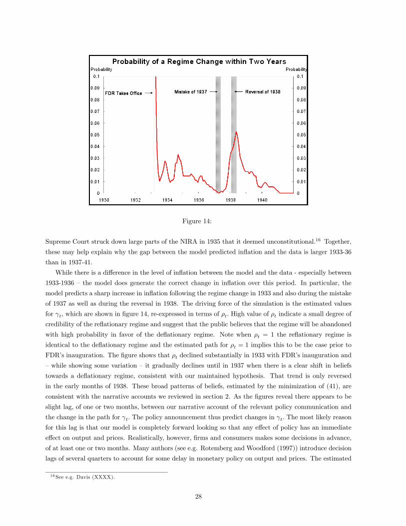
Figure 14:
Supreme Court struck down large parts of the NIRA in 1935 that it deemed unconstitutional.16 Together,
these may help explain why the gap between the model predicted inflation and the data is larger 1933-36
than in 1937-41.
While there is a difference in the level of inflation between the model and the data - especially between
1933-1936 — the model does generate the correct change in inflation over this period. In particular, the
model predicts a sharp increase in inflation following the regime change in 1933 and also during the mistake
of 1937 as well as during the reversal in 1938. The driving force of the simulation is the estimated values
for γt, which are shown in figure 14, re-expressed in terms of ρt. High value of ρt indicate a small degree of
credibility of the reflationary regime and suggest that the public believes that the regime will be abandoned
with high probability in favor of the deflationary regime. Note when ρt = 1 the reflationary regime is
identical to the deflationary regime and the estimated path for ρt = 1 implies this to be the case prior to
FDR’s inauguration. The figure shows that ρt declined substantially in 1933 with FDR’s inauguration and
— while showing some variation — it gradually declines until in 1937 when there is a clear shift in beliefs
towards a deflationary regime, consistent with our maintained hypothesis. That trend is only reversed
in the early months of 1938. These broad patterns of beliefs, estimated by the minimization of (41), are
consistent with the narrative accounts we reviewed in section 2. As the figures reveal there appears to be
slight lag, of one or two months, between our narrative account of the relevant policy communication and
the change in the path for γt. The policy announcement thus predict changes in γt. The most likely reason
for this lag is that our model is completely forward looking so that any effect of policy has an immediate
effect on output and prices. Realistically, however, firms and consumers makes some decisions in advance,
of at least one or two months. Many authors (see e.g. Rotemberg and Woodford (1997)) introduce decision
lags of several quarters to account for some delay in monetary policy on output and prices. The estimated
16See e.g. Davis (XXXX).
28
path for γt, when considered in light of the timing of policy communications, indicate that relatively small
decision lags (of less that one quarter) would be needed to explain a delayed effect of policy surprises on
output and prices during the Great Depression.
7 What was the reason for the mistake of 1937?
In the model it is treated as an exogenous shifts in beliefs, captured by the parameter γt, which we
interpret as a change in the communication about future policy by policymakers, a conjecture supported
by the narrative accounts from newspapers of this period. Left open, however, is why policy makers
choose to send the signals which had this dramatic effects on beliefs and shifted γt. Broadly speaking, one
can hypothesize that either the mistake was (1) unintentional communication of confusing signals or (2)
deliberate (but mistaken) change in policy. Both possibilities can be supported by some evidence, and we
discuss each in turn. While this should be a subject of further study, we believe that in the final analysis,
the most likely explanation is some combination of the two.
The first explanation, that the policy communication was more unintentional than a deliberate change
of course, is more convincing if applied only President Roosevelt than to Federal Reserve policy makers. In
the early months of 1937 FDR was engaged in one of the toughest fights of his career, the "court-packing
fiasco". It was one of the few political battles he would lose during his presidency. FDR was deeply
frustrated with the Supreme Court, because it had been a major obstacle to his reforms, striking down
several New Deal programs as unconstitutional. In response FDR tried to stack the court in 1937 by
proposing legislation that mandated several of the justices to retire due to age. This caused a great furor,
both publicly and within Congress, and had a substantial negative impact on FDR’s credibility. In the
middle of this battle, which started in February 1937, it would have been hard to pay close attention to
monetary policy. Indeed, FDR’s offhand remarks of inflationary dangers on April 2nd, which led to large
market reaction, and that some newspapers would later blame for the depression of 1937-38,17 appear to
be made without much thought or discussion within the administration. Indeed, in 1938, FDR tried to
claim that he had wanted to inflate the price level to pre-depression levels all along, as he had promised
in 1933, despite his explicit warning against too much inflation in April of 1937 . Hence, it is possible to
argue that whatever comments FDR made about inflationary pressures in the spring 1937, they were an
example of confusing signals rather than a genuine change in his thoughts about policy.
What is more certain is that in February 1938 FDR put all his weight and credibility behind a renewed
commitment to reflate. In contrast to his warnings against excessive inflation, this commitment seemed
to have been well thought out and deliberated within the administration. His formal announcement in a
press conference on February 19th was in fact prepared by the joint efforts of the Chairman of the Federal
Reserve and the Secretary of the Treasury, along with several senior advisors.
While one may argue that FDR may have been less than deliberate about the change in course of
policy in the spring of 1937, there appears to be less reason to doubt that the Federal Reserve abruptly
and deliberately changed course during that period (as we document in section 2) The question is why?
The most likely reason is that the Federal Reserve misread the economic situation and focused on a rather
narrow objective for social welfare in a "discretionary way" (in the sense of Kydland and Prescott (1977)).
17 Insert cite from Chicago Tribune.
29
Furthermore, with the passage of the Banking Act of 1935, the Federal Reserve may have seen itself as
no longer bound by FDR’s commitment to inflate the price level to pre-depression levels. To see why
an excessive tightening may have been rational for the Federal Reserve let us suppose that the Federal
Reserve was maximizing social welfare. Under certain conditions (see e.g. Eggertsson (2006a)), the social
welfare function can be approximated by a second order Taylor expansion of the utility of the representative
household yielding∞XT=t
βT−t{π2T + λY 2T }
Consider now the optimal solution from time t onwards under the assumption that the central bank
believes that the natural rate of interest rnt is positive. In this case the Federal Reserve could minimize the
output and inflation at their social optimum, i.e. at πt = Yt = 0 by setting it = rnt > 0. Thus by reneging
on FDR’s 1933 commitment to reflate the price level to pre-depression levels the Federal Reserve could get
a better economic outcome. While this outcome is ex post optimal, it is not optimal ex ante because it
was optimal for the government in 1933 to create expectation about reflation. This ex post incentive to
renege on a previous inflation promise is what Eggertsson (2006a) coins the deflation bias of discretionary
policy. The snag in 1937, of course, is that there is every indication that the Federal Reserve misjudged
the natural rate of interest, believing that the depression was over and that the battle with deflation had
been won. This was a serious misjudgment. Thus, according to this interpretation, the mistake of 1937, as
far as the Federal Reserve was concerned, was a bad miscalculation of actual economic conditions.
8 Conclusion
As always it is difficult to draw strong comparisons between different countries at different times. Japan
today, certainly looks very different form the United States in 1937. Yet there are some similarities and
some lessons that Japanese policy makers may wish to keep in mind. Then most obvious ones that Japan is
also contemplating a transition from zero interest rates to positive ones. The US experience indicates that
economic outcomes can be extremely sensitive to expectations given those circumstances. The highlights the
importance of clear communication by the BoJ about its future inflationary goals as argued by Eggertsson
and Ostry (2005). In particular, the market is very sensitive to signals about the future policy regime.
Given the asymmetries documented in the paper it seems to us more prudent to err on the side of inflation,
rather than deflation.
30
9 References
1. Adam, Klaus and Roberto Billi (2006), “Optimal Monetary Policy under Commitment with a Zero
Bound on Nominal Interest Rates,” Journal of Money, Credit and Banking, forthcoming.
2. Auerbach, Allan, and Maury Obstfeld (2005) "The Case for Open Market Operations," American
Economic Review, Volume 95, No. 1.
3. Calvo, Guillermo. (1983) "Staggered Prices in a Utility-Maximizing Framework," Journal of Mone-
tary Economics, 12: 383-98.
4. Davis, Kenneth, S. (1986) "FDR The New Deal Years 1933-37," New York: Random House.
5. Eccles, Marriner S. (1951) "Beconing Frontiers," New York: Alfred A. Knopf Inc.
6. Eggertsson, Gauti. (2005), "Great Expectations and the End of the Depression," Federal Reserve
Bank of New York, Staff Report no. 234.
7. Eggertsson, Gauti. (2006a), "The Deflation Bias and Committing to Being Irresponsible," Journal
of Money, Credit, and Banking, forthcoming.
8. Eggertsson, Gauti. (2006b), "The New Deal as the Optimal Second Best," Federal Reserve Bank of
New York, mimeo.
9. Eggertsson, Gauti. (2006c), "The Liquidity Trap," the New Palgrave Dictionary of Economics,
forthcoming.
10. Eggertsson, Gauti and Jonathan Ostry (2005) , "Does Excess Liquidity Pose a Threat in Japan?"
IMF Public Policy Paper.
11. Eggertsson, Gauti and Woodford, Michael (2003a), "The Zero Bound on Interest Rates and Optimal
Monetary Policy," Brookings Papers on Economic Activity 1, 212-219.
12. Friedman, Milton and Anna Schwartz. (1963), "A Monetary History of the United States," Princeton
University Press.
13. Jeanne, Olivier and Lars Svensson (2004), "Credible Commitment to Optimal Escape from a Liquidity
Trap: The Role of the Balance Sheet of an Independent Central Bank," mimeo, Princeton University.
14. Keynes, John Maynard. (1936) "The General Theory of Employment Interest and Money", London:
Macmillan.
15. Krugman, Paul. (1998), "It’s Baaack! Japan’s Slump and the return of the Liquidity Trap," Brook-
ings Papers on Economic Activity 2:1998.
16. Kydland, Finn E. and Edward C. Prescott. (1977): "Rules Rather than Discretion: The Inconsistency
of Optimal Plans." J.P.E. (85): 473-91.
17. Meltzer, Allan H. (2003): "A History of the Federal Reserve. Volume 1: 1913-1951", University of
Chicago Press. University of Chicago Press.
31
18. Romer, Christina D. (1992), “What Ended the Great Depression?” Journal of Economic History 52,
December : 757-784.
19. Svensson, Lars (2003), "Escaping from a Liquidity Trap and Deflation: The Foolproof Way and
Others," Journal of Economic Perspectives 17-4, p. 145-166.
20. Telser, L.G. (2001-2002), "Higher member bank reserve rations in 1936 and 1937 did not cause the
relapse into depression," Journal fo Post Keynesian Economics. Vol 24, No. 2, pg.205-216.
21. Woodford, Michael. (2003), "Interest and Prices: Foundations of a Theory of Monetary Policy",
Princeton University.
32