Embed Size (px)
Citation preview
The Long-Run Impact of Monetary Policy on Housing Prices in China
Sherry Yu
New College of Florida
5800 Bay Shore Road
Sarasota, FL 34243
United States
Phone: 941-487-4207
Email: [email protected]
Lini Zhang1
Central University of Finance and Economics
39 Xueyuan South Road
Haidian, Beijing 100081
Phone: (86) 132-4124-7496
Email: [email protected]
Abstract
This paper examines the effect of monetary policy on housing prices in China utilizing a novel set of
housing price indices constructed by Fang et. al (2015). We find that in the long-run, average housing
prices react positively to inflation, money supply, bank lending growth and deposit rate, and negatively to
the reserve requirement ratio, lending rate and retail sales growth. Housing prices in Tier 1 cities are
found to respond more sensitively to monetary shocks relative to Tier 2 and 3 cities. This result may
suggest the presence of market speculation in Tier 1 cities. We further study the volatility effect of
monetary shocks using the GARCH model and find that the reserve requirement ratio and money supply
has strong negative impact on the volatility of housing price growth. These results suggest that monetary
shocks have significant level and volatility effect on housing price growth in China and policymakers
should take consideration of the heterogeneous characteristics of the housing markets in the design of
monetary policy.
Key Words: monetary policy, housing price, monetary shock, volatility
JEL Codes: E2, E4, E5, G1, R3
1 Corresponding author
I. Introduction
The real estate market in China is one of the fastest growing asset markets in the world. Before 1978,
housing stocks were rarely traded as goods under the socialist planned economy. Following the economic
reform and open-door policy, China has transformed into a more competitive market and become a major
driving force of global economic growth over the past few decades. In the mean time, the real estate
market has developed rapidly and become essential for China’s economic growth. Figure 1 displays the
national average monthly housing price growth from 2003 to 2013. Over the decade, housing prices
growth is about 1% per month or about 13% per annum for the country. Also, the housing prices growths
in major cities have been well above the national average. Chen and Wen (2015) reported the average real
housing price in 35 major cities has grown at an annual rate of 17%. Although China enjoyed double-digit
economic growth over the same period, the persistent housing price boom appears puzzling as the housing
prices to income ratio have been climbing and there is a significant urban housing vacancy rate of 22.4%
(Chen and Wen 2015). Researchers have expressed growing concerns over the soaring housing prices as
a market collapse like the 2007 US subprime crisis would bring devastating consequences to the global
economy.
Figure 1. Average Housing Price Index and Monthly Housing Price Growth in China from 2003-2013.
-4
-2
0
2
4
6
0.8
1.0
1.2
1.4
1.6
1.8
2.0
2004 2005 2006 2007 2008 2009 2010 2011 2012 2013
Housing Price Growth % (Left Axis)
Housing Price Index (Right Axis)
Source: Data is taken from Fang et al. (2015).
Since the 2007 financial crisis, researchers that actively study the cause and aftermath of the recent
global recession have found nontrivial roles of the central banks in the prevention and restoration of crisis.
Brunnermeier (2009) finds that a period of low interest rate and declining lending standards may have set

the foundation for the subprime crisis in 2007. Mishkin (2011) further evaluates the actions taken by the
Federal Reserve over the course of the crisis and concludes that government actions have helped to
prevent a far deeper recession in the global economy. Since China has become a major growth engine to
the global economy and the Chinese housing market share similarities to the US housing market before
the crisis, it is important to understand the Chinese housing market and evaluate the effectiveness of
monetary policy to housing prices. Nevertheless, a limited number of papers have explored the impact of
monetary policy on housing prices and its volatility. Due to lack of reliable data samples, the existing
studies have not provided consistent results and require further examination. Moreover, the economic and
housing development in China is heterogeneous across different areas in the country, but no research have
examined the relationship between monetary policy and housing prices considering the heterogeneity of
economic conditions.
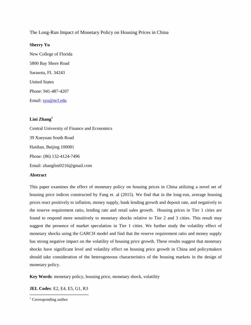
Figure 2. Money Supply and Bank Lending Growth in China from 2003-2013.
-0.5
0.0
0.5
1.0
1.5
2.0
2.5
4.2
4.4
4.6
4.8
5.0
5.2
2004 2005 2006 2007 2008 2009 2010 2011 2012 2013
Bank Lending Growth Rate % (Left Axis)
Money Supply M2 (log, Right Axis)
Source: Data is taken from the CEIC Database.
To address these concerns and study the implication of monetary measures on the housing market and
integrate the heterogeneous characteristics of urban cities into our study, we develop an empirical
framework based on relatively more reliable monetary and housing data to answer three questions. First,
what were the long-run and short-run effects of monetary policy on the rapidly appreciating housing
prices? Second, how did the impact of monetary shocks on the housing market vary across different types
of Chinese cities? Third, was there evidence of market speculation that may lead to a large-scale
meltdown? We seek to address these questions by studying the long-run relationship between monetary

policies and housing price growth in China, with special focus on the heterogeneous characteristics of
different tiers of cities in the country.
Our monthly data samples concerning the monetary policy and macroeconomic conditions are from the
CEIC database, which contains official statistics released by the National Bureau of Statistics on a
periodical basis. There have been traditional concerns over the accuracy and integrity of the official
housing price data published by the National Bureau of Statistics of China. Deng, Gyourko and Wu
(2014) criticize the data to be overly smooth with little housing price growth in the recent decade. To
avoid this problem, we utilize a novel set of housing price indices compiled by Fang, Gu, Xiong and Zhu
(2015). Using the new home sales prices in 120 major cities in China, Fang et al (2015) provides a
unique approach to individually track housing price movements using mortgage and sequential sales data.
For example, the sales prices of the same condominium project are monitored on a monthly basis from
2003 to 2013. This unique approach provides invaluable high-frequency data that more accurately reflects
significant price appreciation and volatility that are otherwise muted in the official data. In addition,
comparing to other unofficial housing price indices, the indices compiled by Fang et al (2015) are more
superior in terms of data length, data frequency, the coverage of major cities, and the data construction
method.
Moreover, many existing researches solely rely on money supply (M2) to represent the stance of
China’s monetary policy (see Fernald et al. (2014), Koivu (2010)), which may provide limited scope as
the PBC adopts a variety of alternative instruments for monetary control. To address this issue, we
consider five alternative monetary measures including the benchmark deposit rate, benchmark lending
rate, money supply (M2), bank reserve requirement and bank lending growth rate from January 2003 to
January 2013. We include all relevant monetary measures that are targeted by the PBC in our estimation
because the PBC may not be able to accurately target money supply in the short run. A more
comprehensive set of monetary instruments can allow us to have more robust short-run and long-run
estimations. Figure 2 displays the rapid expansion of money supply and bank lending in China over the
same period. We also include inflation, consumption and retail sales to capture the variation of
macroeconomic conditions in China. Finally, considering the heterogeneity in China’s economic
development, we divide 101 major Chinese cities into three tiers. Such division allows us to study the
sensitivity of housing prices responses to monetary shocks in cities that share similar economic
characteristics.
We study the long-run effect of monetary policy measures on housing price growth using the
Autoregressive Distributed Lag (ARDL) model and further investigate the short-run dynamics using the
traditional error-correction model. Khemraj and Yu (2016) uses similar approach to assess the effect of

large-scale asset purchase programs implemented by the Fed on the level of investments in the United
States. We hypothesize that expansionary monetary policy such as decreasing benchmark interest rates,
money supply growth and lowering reserve requirement ratio would have positive effect on housing price
growth. In addition, the soaring property prices in Tier 1 cities would imply a tighter budget constraint for
buyers associated with a greater reliance on credit lending. Thus we hypothesize that the housing price
growths in Tier 1 cities would be more sensitive to monetary shocks than Tier 2 and 3 cities.
Our paper is also one of the first to study the monetary effect on the volatility of housing price
movements in China. We use the traditional Generalized Autoregressive Conditional Heteroscedasticity
(GARCH) process to study the effect of monetary policy shocks on the risk and uncertainty in the real
estate market. Our results are mixed. We first find that expansionary policy such as money supply growth
reduces the general volatility of the housing price movements. Nonetheless, we also find that a
contractionary policy in the form of increased bank reserve requirement also reduces uncertainty in the
market. This may be caused by the different perception and interpretation investors have regarding
different types of monetary instrument. Furthermore, we find tentative evidence of the existence of
market speculation in Tier 1 cities as the volatility of housing price growth is largely unaffected by
monetary policy shocks. This may imply that investors evaluate the risk and uncertainty in these markets
using other factors such as land supply and home purchase policies. Comparatively, money supply growth
negatively affects the volatility of housing price changes in Tier 2 and 3 cities.
Our research has a few limitations due to the availability of data. First, land prices may have affected
the housing prices but were excluded from our model since the national and metropolitan land prices were
undisclosed to the public. Newspapers may report land prices on an infrequent basis, but they would not
provide sufficient time series data for our analysis. Second, we may have excluded some government
interventions in the housing market in our analysis. We address this issue by considering the home-
purchase restrictions imposed by the government in the robustness test. A large number of economists
believe that the home-purchase restrictions may have affected the housing prices as it could reduce the
housing demand. After we introduced the policy dummy, we find that our benchmark results remain
robust and the home-purchase restrictions have negative and significant effect on housing price growth.
Moreover, monthly data on macroeconomic variables such as consumption and retail sales are not
available at the city level. The lack of city-level data eliminates the possibility of a panel data analysis. As
a result, we utilize time series estimation and do not separately identify city-level monetary shocks in our
analysis. Lastly, our empirical analysis may be subject to endogeneity problem due to the bi-directional
relationship between business cycle indicators and monetary shocks. To alleviate this potential issue, we
exclude the more popular GDP and disposable income measures that appear to be directly related to

monetary policy shocks and choose consumption and retail sales data as a proxy for macroeconomic
conditions in China.
The rest of the paper is organized as follows. Section II reviews the relevant literature and section III
explains the data and methodology used in this paper. Section IV evaluates the empirical results and
section V studies the heterogeneous nature of China’s housing market. Section VI shows robustness test.
Section VII concludes.
II. Literature Review
As an important growth engine in the world, the monetary policy rules, instruments and transmission
mechanism in China have been extensively studied. Fernald, Spiegel and Swanson (2014) adopt the
FAVAR approach and find that the required reserve ratio and interest rates have been effective on
economic activity and inflation in China. Chen, Chen and Gerlach (2011) find that the People's Bank of
China (PBC) mainly uses the required reserve ratios and open market operations to affect liquidity in
money markets. The PBC adjusts deposit and lending rates to intervene the retail deposit and lending
market. Kim and Shi (2014) find that the PBC respond to changes in inflation and money growth by
revising the benchmark deposit rate and lending rate. Girardin, Lunven and Ma (2014) find that the
Chinese monetary policy is similar to implicit flexible inflation targeting. The monetary policy is forward
looking and has high output weight typical of emerging economies. Based on the results from existing
studies, we use required reserve ratio, M2 and benchmark lending rate and deposit to represent the stance
of the Chinese monetary policy in our paper. We further extend our studies to explore the effects of
monetary policy on house prices.
Our paper is also related to the literature on house prices and the stance of monetary policy. Based on
different estimation methods and data samples, a large number of papers have found that monetary policy
can have significant effects on house prices in the United States, the United Kingdom and other major
industrial countries. Leading examples are Jarocinksi and Smets (2008), John C. Williams (2015),
Ahearne, Ammer, Doyle, Kole and Martin (2005), and Elboune (2008). Departing from these papers, we
study the effects of monetary policy on house prices in China. Consistent with their findings, we find that
monetary policy has significant effects on house prices in China.
A limited number of papers have explored the impact of monetary policy on house prices in China.
Using the CEIC database, Koivu (2010) estimates a structural VAR model and finds that monetary policy
has an impact on stock and residential housing prices in China, but the link from monetary policy to
household consumption is weak. Xu and Chen (2012) point out that Chinese monetary policy are the key
driving forces behind the house prices growth. Tan and Chen (2013) evaluates whether the PBC should
react to house prices and if so how. Yao et al (2013) find monetary policies have little immediate effect
on asset prices. Contrasting to these studies, our research has three major innovations. First, we utilize a
new set of house prices indices constructed by Fang et al. (2015) to avoid the underestimation problem
associated with the official Chinese house prices data. Second, we study the sensitivity of housing prices
responses to monetary shocks in three tiers of Chinese cities that share similar economic characteristics.
Third, we include a more comprehensive set of monetary measures targeted by the PBC in our estimation.
Besides examining the level effect of monetary policy on house prices in both the short-run and long-
run, we also find significant volatility effect of monetary shocks using the GARCH model. In contrast, a
few existing literature have studied the driving forces of price volatility and no previous paper has found
that monetary policy has significant impact on house price volatility. Kuang (2010) studies the effect of
speculation on housing price volatility and finds that adaptive expectation, housing income, population
growth and actual interest rates are significant factors. He further finds that housing price volatility does
not vary across cities. Deng et al. (2015) uses sequential modeling to study the determining forces of
housing price volatility in Beijing and Shanghai and find that hedonic characteristics and economic
fundamentals are significant but monetary policy appears to be unrelated to the long-run price volatility.
Wang and Han (2009) use GARCH mean-value equation model to analyze volatility correlations between
money supply, economic growth and housing price and find little evidence of the effect of real estate
price volatility on GDP growth and the comovements between money supply and housing price change
rapidly in the beginning of the 21st century. Based on more reliable data sets, our paper depart from theirs
to study both the long-run and short-run effect of monetary policy on housing prices and volatility, with a
special focus on the heterogeneous responses in the three different tiers of cities. To the best of our
knowledge, we are the first to find significant effects of monetary policy on housing price growth
volatility in China. This significant finding may be attributed to the utilization of a more accurate set of
monthly housing price indices in our study.
III. Data and Methodology
Data
We study the long-term and short-term effect of monetary shocks on the housing prices using five
monetary measures including the PBC’s benchmark lending rate, benchmark deposit rate, reserve
requirement, commercial bank lending growth, and money supply. We use the M2 measure for money
supply that is consistent with the existing literature (see Fernald, Spiegel and Swanson, 2014 for a
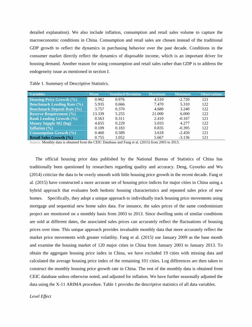
detailed explanation). We also include inflation, consumption and retail sales volume to capture the
macroeconomic conditions in China. Consumption and retail sales are chosen instead of the traditional
GDP growth to reflect the dynamics in purchasing behavior over the past decade. Conditions in the
consumer market directly reflect the dynamics of disposable income, which is an important driver for
housing demand. Another reason for using consumption and retail sales rather than GDP is to address the
endogeneity issue as mentioned in section I.
Table 1. Summary of Descriptive Statistics.
Variables Mean Standard Deviation Maximum Minimum Observations
Housing Price Growth (%) 0.982 0.976 4.510 -2.720 121
Benchmark Lending Rate (%) 5.935 0.666 7.470 5.310 122
Benchmark Deposit Rate (%) 3.757 0.370 4.680 3.240 122
Reserve Requirement (%) 13.339 5.255 21.000 6.000 122
Bank Lending Growth (%) 0.563 0.311 2.410 -0.167 121
Money Supply M2 (log) 4.655 0.229 5.033 4.277 122
Inflation (%) 0.109 0.183 0.835 -0.395 122
Consumption Growth (%) 0.460 0.589 3.618 -2.450 121
Retail Sales Growth (%) 0.755 1.052 5.667 -3.136 121 Source: Monthly data is obtained from the CEIC Database and Fang et al. (2015) from 2003 to 2013.
The official housing price data published by the National Bureau of Statistics of China has
traditionally been questioned by researchers regarding quality and accuracy. Deng, Gyourko and Wu
(2014) criticize the data to be overly smooth with little housing price growth in the recent decade. Fang et
al. (2015) have constructed a more accurate set of housing price indices for major cities in China using a
hybrid approach that evaluates both hedonic housing characteristics and repeated sales price of new
homes. Specifically, they adopt a unique approach to individually track housing price movements using
mortgage and sequential new home sales data. For instance, the sales prices of the same condominium
project are monitored on a monthly basis from 2003 to 2013. Since dwelling units of similar conditions
are sold at different dates, the associated sales prices can accurately reflect the fluctuations of housing
prices over time. This unique approach provides invaluable monthly data that more accurately reflect the
market price movements with greater volatility. Fang et al. (2015) use January 2009 as the base month
and examine the housing market of 120 major cities in China from January 2003 to January 2013. To
obtain the aggregate housing price index in China, we have excluded 19 cities with missing data and
calculated the average housing price index of the remaining 101 cities. Log differences are then taken to
construct the monthly housing price growth rate in China. The rest of the monthly data is obtained from
CEIC database unless otherwise noted, and adjusted for inflation. We have further seasonally adjusted the
data using the X-11 ARIMA procedure. Table 1 provides the descriptive statistics of all data variables.
Level Effect
We first examine the level effect of monetary shocks on housing price growth in China using the
ARDL bounds testing approach suggested by Pesaran, Shin and Smith (2001). The ARDL bounds testing
approach has several advantages over traditional methods. First, it estimates the cointegration relationship
using the OLS method with optimal lags. In addition, the model allows for the presence of both I(0) and
I(1) variables as oppose to alternative methods such as Johansen and Juselius (1990). This minimizes the
potential issue that the results may be sensitive to the choice of unit root tests when determining the order
of integration for each variable. Nonetheless, the model is not applicable with the presence of I(2)
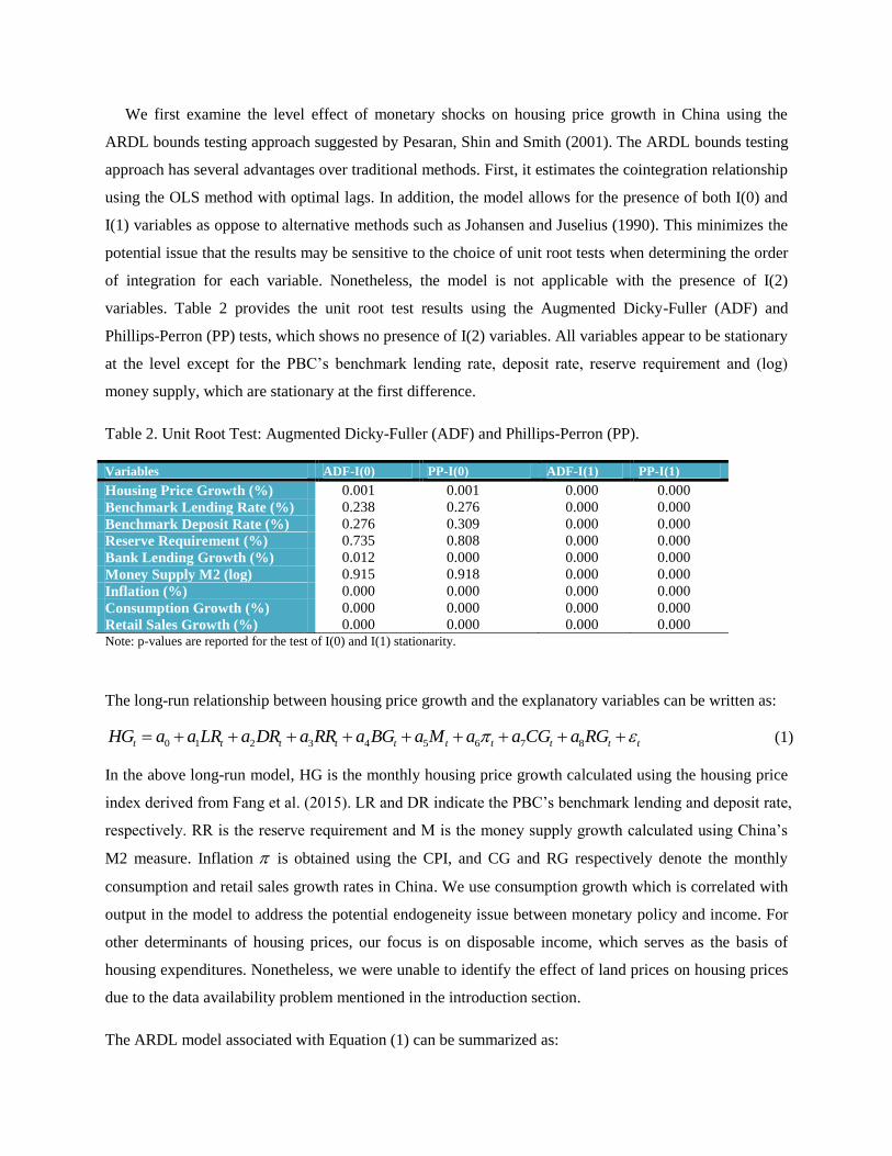
variables. Table 2 provides the unit root test results using the Augmented Dicky-Fuller (ADF) and
Phillips-Perron (PP) tests, which shows no presence of I(2) variables. All variables appear to be stationary
at the level except for the PBC’s benchmark lending rate, deposit rate, reserve requirement and (log)
money supply, which are stationary at the first difference.
Table 2. Unit Root Test: Augmented Dicky-Fuller (ADF) and Phillips-Perron (PP).
Variables ADF-I(0) PP-I(0) ADF-I(1) PP-I(1)
Housing Price Growth (%) 0.001 0.001 0.000 0.000
Benchmark Lending Rate (%) 0.238 0.276 0.000 0.000
Benchmark Deposit Rate (%) 0.276 0.309 0.000 0.000
Reserve Requirement (%) 0.735 0.808 0.000 0.000
Bank Lending Growth (%) 0.012 0.000 0.000 0.000
Money Supply M2 (log) 0.915 0.918 0.000 0.000
Inflation (%) 0.000 0.000 0.000 0.000
Consumption Growth (%) 0.000 0.000 0.000 0.000
Retail Sales Growth (%) 0.000 0.000 0.000 0.000 Note: p-values are reported for the test of I(0) and I(1) stationarity.
The long-run relationship between housing price growth and the explanatory variables can be written as:
0 1 2 3 4 5 6 7 8t t t t t t t t t tHG a a LR a DR a RR a BG a M a a CG a RG (1)
In the above long-run model, HG is the monthly housing price growth calculated using the housing price
index derived from Fang et al. (2015). LR and DR indicate the PBC’s benchmark lending and deposit rate,
respectively. RR is the reserve requirement and M is the money supply growth calculated using China’s
M2 measure. Inflation is obtained using the CPI, and CG and RG respectively denote the monthly
consumption and retail sales growth rates in China. We use consumption growth which is correlated with
output in the model to address the potential endogeneity issue between monetary policy and income. For
other determinants of housing prices, our focus is on disposable income, which serves as the basis of
housing expenditures. Nonetheless, we were unable to identify the effect of land prices on housing prices
due to the data availability problem mentioned in the introduction section.
The ARDL model associated with Equation (1) can be summarized as:
31 2
5 6 7 8 94
0
1 1 1
1
1 1 1 1 1 1
2 3 4 5 6 7 8 9
nn n
t j t j j t j j t j
j j j
n n n n nn
j t j j t j j t j j t j j t j j t j t
j j j j j j
t t t t t t t t t
HG b HG c LR d DR
e RR f BG g M h i CG k RG HG
LR DR RR BG M CG RG
(2)
The null hypothesis of no co-integration 0 1 2 3 4 5 6 7 8 9: 0H is
tested against the alternative 1 1 2 3 4 5 6 7 8 9: 0H using an F-test. The
ARDL bounds testing examines the two critical asymptotic values: an upper value assuming all regressors
are I(1) and a lower value with the assumption that all variables are I(0). The null hypothesis that no
cointegration relationship exists can be rejected if the F-statistics is above the upper bound but cannot be
rejected if it falls below the lower bound. The test is inconclusive if the F-statistics falls in between the
two critical values.
If the null hypothesis is rejected, we can then estimate the long-run equilibrium relationship between
housing price growth and the explanatory variables as outlined in Equation (1), and the short-term error
correction model given by:
31 2
5 6 7 8 94
0
1 1 1
1
1 1 1 1 1 1
nn n
t j t j j t j j t j
j j j
n n n n nn
j t j j t j j t j j t j j t j j t j t t
j j j j j j
HG b HG c LR d DR
e RR f BG g M h i CG k RG z
(3)
1tz is the error correction term from the long-run model and represents the speed of convergence of
short-run dynamics to the equilibrium. The long-run effects can be extracted then using this unrestricted
error correction model.
Volatility Effect
China’s real estate market is often viewed as speculative and “bubble” forming, with high degree of
volatility and uncertainty (Chen and Wen, 2015). Rapid growth in housing prices across China may have
been contributed by the strong economic fundamentals, but monetary policy could also affect investors’
perception of risk and uncertain in the market. There have been relatively few researches (see Deng et al.,
2015 for a review) on the determining factors of price fluctuations and this paper attempts to fill in the
gap by examining the effect of monetary policy on housing price volatility using the GARCH model.
Volatility is commonly used as a proxy for uncertainty. For instance, the Volatility Index of S&P 500
(VIX) spiked in 2008 amid great turbulence in the financial markets. In the real estate market, volatility
may be used to assess the degree of market uncertainty and speculation. In periods of high speculation,
price changes may be more volatile as the market contains a high degree of uncertainty. Monetary policy
could potential play a vital role in driving market sentiment and may be tightly linked to housing price
volatility in China.
We investigate the effect of monetary policy on the volatility of housing price growth rates using the
GARCH model. The first and second moments of a GARCH (p,q) model can be expressed as:
't t tY X (4)
2 2 2
1 1
p q
t i t i j t j
j j
(5)
Equation (4) is the mean equation of the model expressed as a function of exogenous variables, tX and an
error term, t . Equation (5) characterizes the current period conditional variance,2
t as a function of
previous periods’ news on volatility 2
t i and forecast variance
2
t j . A best-fitting GARCH model is
selected using the Akaike Information Criterion (AIC).
IV. Empirical Results
ARDL Bounds Test
We examine the long-run cointegrating relationship between housing price growth and monetary
policy measures using the ARDL bounds testing approach proposed by Pesaran, Shin and Smith (2001).
We estimate the model specified in Equation (2) using monthly data from 2003 to 2013 and impose a
maximum amount of 6 lags. The optimal number of lags for each variable is then selected using the AIC
method. We further run the LM, normality and heteroscedasticity tests to confirm that there is no
evidence of serial correlation in the residuals. The F-statistics reported is 5.583, which exceeds the upper
bound of 3.77 with 1% significance level as provided in Pesaran, Shin and Smith (2001). This implies
that housing price growth and our explanatory variables have cointegrating relationships in the long-run
and we can then assess the level effect of monetary shocks on the housing price movement. The reported
adjusted R2 is 0.75 and the coefficient for the error correction term, = −0.361 is negative and significant
at the 1% level. This coefficient measures the speed of adjustment from the short-run to the long-run
equilibrium, and must fall between -1 and 0 for a correctly specified model. Our results show that the
model is valid and the short-run housing prices in China adjust at a moderate rate to the long-run
equilibrium.

The long-run relationship for the ARDL model characterized by Equation (1) can be written as:
*** * * ***
(0.116) (0.446) (0.762) (0.118) (1.042)
* *** **
(0.026) (2.840) (0.205) (0.256)
0.160 1.536 1.439 0.229 2.754
0.046 11.962 0.339 0.508
t t t t t
t t t t
HG LR DR RR BG
M CG RG
(6)
Asterisks are used to denote the significant level where *p<0.1, **p<0.05, ***p<0.01. In the long-run,
lending rate, reserve requirement ratio and retail sales growth negatively affect the average housing price
growth in China. This is consistent with our hypothesis that when monetary policy is tightened by
increasing PBC’s benchmark lending rate and reserve requirement ratio, the availability of funds in the
market decreases and asserts negative pressure on the housing prices. In addition, demand for housing is
also tied to disposable income. As households consume more retail goods, the disposable income
available for housing stock purchases decline and negatively affects the housing price growth in China. In
general, expansionary monetary policy positively and significantly affects housing price growth. Our
results show that housing price growth increase with the bank lending growth rate and money supply,
along with inflation and the benchmark deposit rate. Inflation has the strongest effect on housing price
growth in the long-run, which is consistent with the existing literature. The deposit rate in China has long
been flat as the central bank has been using low rate to channel cheap credit to the state-owned enterprises.
In the long-run, households may interpret a rising deposit rate as a sign of positive economic growth in
China and demand more housing stock as a form of investment.
We further examine the short-run effect of monetary policy on housing price growth to study how the
real estate market adjusts to temporary shocks in the economy. The short-run error correction
representation characterized by Equation (3) can be rewritten as:
*** ** **
1 2 3(0.040) (0.088) (0.100) (0.080) (0.424)
***
1 1 2(0.423) (0.371) (0.500) (0.478) (0.040)
0.058 0.698 0.238 0.178 0.143
0.699 0.248 0.494 1.330 0.083
t t t t t
t t t t
HG HG HG HG LR
LR DR DR DR R
**
*** * *
1 2 3(0.184) (0.177) (0.177) (0.155) (0.009)
* ***
1 2 3(0.262) (0.292) (0.271) (0.271) (0.288)
0.052 0.075 0.744 0.275 0.017
0.316 0.552 0.236 0.924 0.471
t
t t t t t
t t t t t
R
BG BG BG BG M
***
4 5(0.281)
*** *** ***
6 1 1(0.279) (0.076) (0.046) (0.047) (0.047)
0.752
1.078 0.123 0.058 0.125 0.361
t
t t t t tCG RG RG z
(7)
Standard errors are reported in parentheses and the term 1tz represents the cointegration term of the
model. The housing price growth rate shows self-adjustment process as it reacts positively to the first-
month and third-month lags, but negatively to the second-month lag. Of the five monetary policy
measures we consider, only lending rate appears to have no short-run effect on housing price growth.
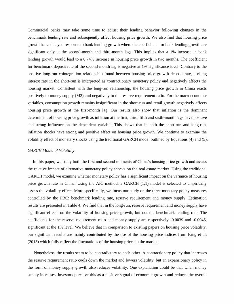
Commercial banks may take some time to adjust their lending behavior following changes in the
benchmark lending rate and subsequently affect housing price growth. We also find that housing price
growth has a delayed response to bank lending growth where the coefficients for bank lending growth are
significant only at the second-month and third-month lags. This implies that a 1% increase in bank
lending growth would lead to a 0.74% increase in housing price growth in two months. The coefficient
for benchmark deposit rate of the second-month lag is negative at 1% significance level. Contrary to the
positive long-run cointegration relationship found between housing price growth deposit rate, a rising
interest rate in the short-run is interpreted as contractionary monetary policy and negatively affects the
housing market. Consistent with the long-run relationship, the housing price growth in China reacts
positively to money supply (M2) and negatively to the reserve requirement ratio. For the macroeconomic
variables, consumption growth remains insignificant in the short-run and retail growth negatively affects
housing price growth at the first-month lag. Our results also show that inflation is the dominant
determinant of housing price growth as inflation at the first, third, fifth and sixth-month lags have positive
and strong influence on the dependent variable. This shows that in both the short-run and long-run,
inflation shocks have strong and positive effect on housing price growth. We continue to examine the
volatility effect of monetary shocks using the traditional GARCH model outlined by Equations (4) and (5).
GARCH Model of Volatility
In this paper, we study both the first and second moments of China’s housing price growth and assess
the relative impact of alternative monetary policy shocks on the real estate market. Using the traditional
GARCH model, we examine whether monetary policy has a significant impact on the variance of housing
price growth rate in China. Using the AIC method, a GARCH (1,1) model is selected to empirically
assess the volatility effect. More specifically, we focus our study on the three monetary policy measures
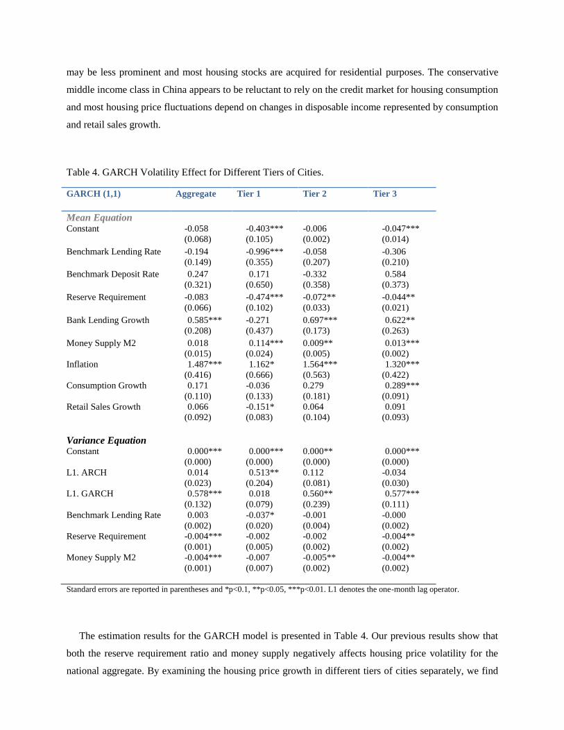
controlled by the PBC: benchmark lending rate, reserve requirement and money supply. Estimation
results are presented in Table 4. We find that in the long-run, reserve requirement and money supply have
significant effects on the volatility of housing price growth, but not the benchmark lending rate. The
coefficients for the reserve requirement ratio and money supply are respectively -0.0039 and -0.0045,
significant at the 1% level. We believe that in comparison to existing papers on housing price volatility,
our significant results are mainly contributed by the use of the housing price indices from Fang et al.
(2015) which fully reflect the fluctuations of the housing prices in the market.
Nonetheless, the results seem to be contradictory to each other. A contractionary policy that increases
the reserve requirement ratio cools down the market and lowers volatility, but an expansionary policy in
the form of money supply growth also reduces volatility. One explanation could be that when money
supply increases, investors perceive this as a positive signal of economic growth and reduces the overall

uncertainty in the financial market followed by a decrease in volatility of housing price growth. However,
the reserve requirement ratio is perceived to be tightly connected to funds availability in the housing
market. When the ratio is lowered, investors’ budget constraints are relaxed leading to an expansion in
housing stock acquisition that pushes up the volatility in housing price growth. In addition, this may
induce uncertainty about future changes in reserve requirement that could alter the conditions of the
mortgage market substantially. For the mean equation, bank lending growth and inflation have strong and
positive influence on housing price growth, consistent with the results from the ARDL model.
V. The 3-Tier Divide
Our paper investigates the heterogeneous characteristics of China’s housing market by examining the
effect of monetary policy on the housing price growth rates in different tiers of cities. Figure 3 shows that
the housing price growth varies significantly across different tiers of cities with Tier 1 in strong
dominance over the others. We utilize the same empirical framework to study the distinctive features in
each type of cities and assess the relative sensitivity of housing price in response to monetary and
macroeconomic shocks.
The first tier refers to the most active housing markets in China that includes Beijing, Shanghai,
Shenzhen and Guangzhou. These four cities maintained leading GDP growth over the past decade and
have traditionally been the “hot” market for real estate investment. The land supply in the first tier cities
is significantly limited while the housing demand is strong as migrants from other areas establish
permanent residences in these cities. In these cities, a significant portion of housing stock is traded as a
form of investment. Fang et al. (2015) find that in 2013, about 11% of all mortgage loans were second
mortgages to fund investment housing purchases in Tier 1 cities, compared to only 3.3% and 1.8% in Tier
2 and 3 cities, respectively. We hypothesize that in Tier 1 cities, housing prices are more sensitive to
monetary policy and macroeconomic variables in both the short-run and long-run. Housing purchases in
Tier 1 cities also rely more extensively on bank credit as the price-to-income ratio is high. Thus housing
price growth in Tier 1 cities should exhibit the greatest sensitivity to monetary policy relative to other
cities.
Tier 2 cities refer to 28 large metropolitan areas that include provincial capitals and two autonomous
cities (Tianjin and Chongqing). These cities are generally less active than the first tier cities but are
considered regional hotspots for investments. Housing demand largely comes from local residents and
migrants from surrounding areas seeking permanent residence in the process of urbanization. The
distinctive nature of Tier 2 cities is the low utilization of credit market for housing consumption. Fang et
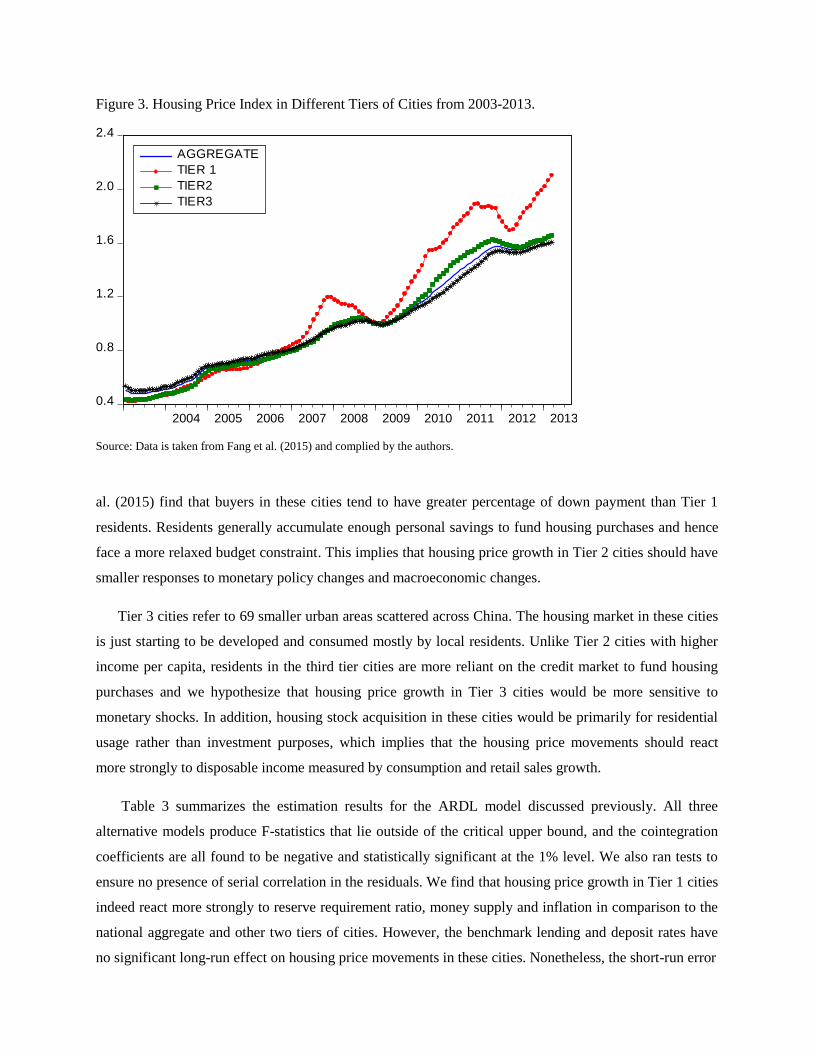
Figure 3. Housing Price Index in Different Tiers of Cities from 2003-2013.
0.4
0.8
1.2
1.6
2.0
2.4
2004 2005 2006 2007 2008 2009 2010 2011 2012 2013
AGGREGATE
TIER 1
TIER2
TIER3
Source: Data is taken from Fang et al. (2015) and complied by the authors.
al. (2015) find that buyers in these cities tend to have greater percentage of down payment than Tier 1
residents. Residents generally accumulate enough personal savings to fund housing purchases and hence
face a more relaxed budget constraint. This implies that housing price growth in Tier 2 cities should have
smaller responses to monetary policy changes and macroeconomic changes.
Tier 3 cities refer to 69 smaller urban areas scattered across China. The housing market in these cities
is just starting to be developed and consumed mostly by local residents. Unlike Tier 2 cities with higher
income per capita, residents in the third tier cities are more reliant on the credit market to fund housing
purchases and we hypothesize that housing price growth in Tier 3 cities would be more sensitive to
monetary shocks. In addition, housing stock acquisition in these cities would be primarily for residential
usage rather than investment purposes, which implies that the housing price movements should react
more strongly to disposable income measured by consumption and retail sales growth.
Table 3 summarizes the estimation results for the ARDL model discussed previously. All three
alternative models produce F-statistics that lie outside of the critical upper bound, and the cointegration
coefficients are all found to be negative and statistically significant at the 1% level. We also ran tests to
ensure no presence of serial correlation in the residuals. We find that housing price growth in Tier 1 cities
indeed react more strongly to reserve requirement ratio, money supply and inflation in comparison to the
national aggregate and other two tiers of cities. However, the benchmark lending and deposit rates have
no significant long-run effect on housing price movements in these cities. Nonetheless, the short-run error
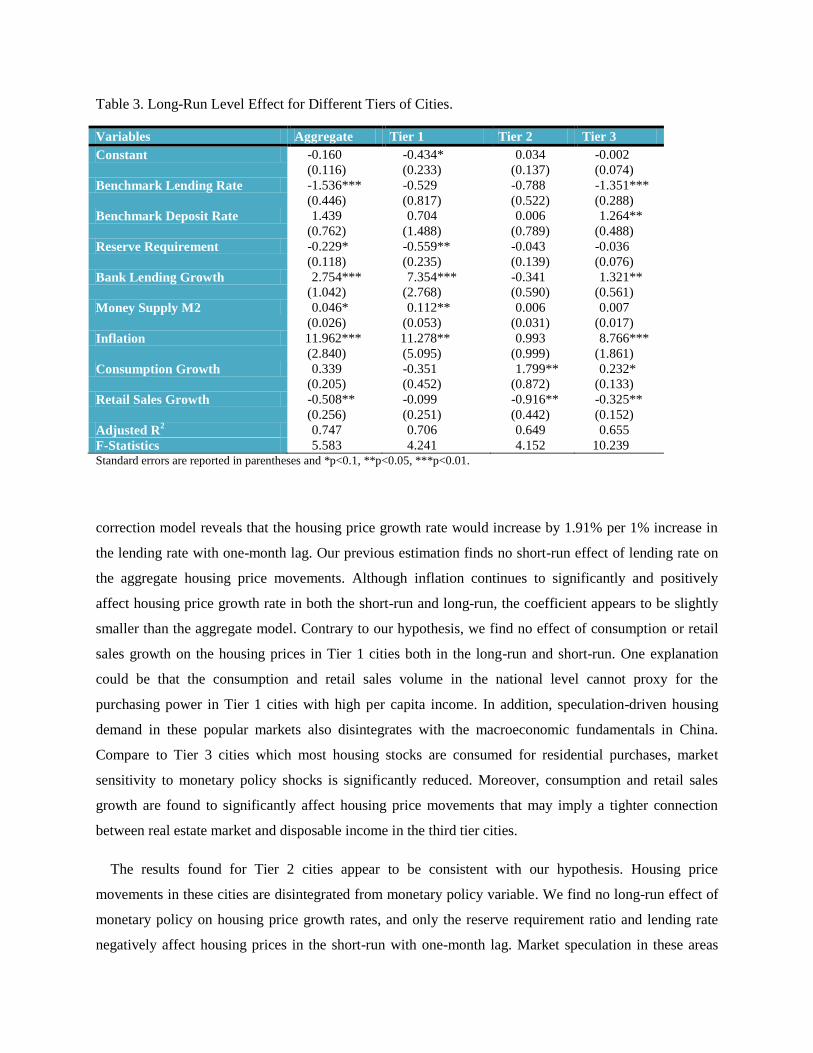
Table 3. Long-Run Level Effect for Different Tiers of Cities.
Variables Aggregate Tier 1 Tier 2 Tier 3
Constant -0.160
(0.116)
-0.434*
(0.233)
0.034
(0.137)
-0.002
(0.074)
Benchmark Lending Rate -1.536***
(0.446)
-0.529
(0.817)
-0.788
(0.522)
-1.351***
(0.288)
Benchmark Deposit Rate 1.439
(0.762)
0.704
(1.488)
0.006
(0.789)
1.264**
(0.488)
Reserve Requirement -0.229*
(0.118)
-0.559**
(0.235)
-0.043
(0.139)
-0.036
(0.076)
Bank Lending Growth 2.754***
(1.042)
7.354***
(2.768)
-0.341
(0.590)
1.321**
(0.561)
Money Supply M2 0.046*
(0.026)
0.112**
(0.053)
0.006
(0.031)
0.007
(0.017)
Inflation 11.962***
(2.840)
11.278**
(5.095)
0.993
(0.999)
8.766***
(1.861)
Consumption Growth 0.339
(0.205)
-0.351
(0.452)
1.799**
(0.872)
0.232*
(0.133)
Retail Sales Growth -0.508**
(0.256)
-0.099
(0.251)
-0.916**
(0.442)
-0.325**
(0.152)
Adjusted R2 0.747 0.706 0.649 0.655
F-Statistics 5.583 4.241 4.152 10.239 Standard errors are reported in parentheses and *p<0.1, **p<0.05, ***p<0.01.
correction model reveals that the housing price growth rate would increase by 1.91% per 1% increase in
the lending rate with one-month lag. Our previous estimation finds no short-run effect of lending rate on
the aggregate housing price movements. Although inflation continues to significantly and positively
affect housing price growth rate in both the short-run and long-run, the coefficient appears to be slightly
smaller than the aggregate model. Contrary to our hypothesis, we find no effect of consumption or retail
sales growth on the housing prices in Tier 1 cities both in the long-run and short-run. One explanation
could be that the consumption and retail sales volume in the national level cannot proxy for the
purchasing power in Tier 1 cities with high per capita income. In addition, speculation-driven housing
demand in these popular markets also disintegrates with the macroeconomic fundamentals in China.
Compare to Tier 3 cities which most housing stocks are consumed for residential purchases, market
sensitivity to monetary policy shocks is significantly reduced. Moreover, consumption and retail sales
growth are found to significantly affect housing price movements that may imply a tighter connection
between real estate market and disposable income in the third tier cities.
The results found for Tier 2 cities appear to be consistent with our hypothesis. Housing price
movements in these cities are disintegrated from monetary policy variable. We find no long-run effect of
monetary policy on housing price growth rates, and only the reserve requirement ratio and lending rate
negatively affect housing prices in the short-run with one-month lag. Market speculation in these areas
may be less prominent and most housing stocks are acquired for residential purposes. The conservative
middle income class in China appears to be reluctant to rely on the credit market for housing consumption
and most housing price fluctuations depend on changes in disposable income represented by consumption
and retail sales growth.
Table 4. GARCH Volatility Effect for Different Tiers of Cities.
GARCH (1,1) Aggregate Tier 1 Tier 2 Tier 3
Mean Equation
Constant -0.058
(0.068)
-0.403***
(0.105)
-0.006
(0.002)
-0.047***
(0.014)
Benchmark Lending Rate -0.194
(0.149)
-0.996***
(0.355)
-0.058
(0.207)
-0.306
(0.210)
Benchmark Deposit Rate 0.247
(0.321)
0.171
(0.650)
-0.332
(0.358)
0.584
(0.373)
Reserve Requirement -0.083
(0.066)
-0.474***
(0.102)
-0.072**
(0.033)
-0.044**
(0.021)
Bank Lending Growth 0.585***
(0.208)
-0.271
(0.437)
0.697***
(0.173)
0.622**
(0.263)
Money Supply M2
0.018
(0.015)
0.114***
(0.024)
0.009**
(0.005)
0.013***
(0.002)
Inflation
1.487***
(0.416)
1.162*
(0.666)
1.564***
(0.563)
1.320***
(0.422)
Consumption Growth
0.171
(0.110)
-0.036
(0.133)
0.279
(0.181)
0.289***
(0.091)
Retail Sales Growth
0.066
(0.092)
-0.151*
(0.083)
0.064
(0.104)
0.091
(0.093)
Variance Equation
Constant
0.000***
(0.000)
0.000***
(0.000)
0.000**
(0.000)
0.000***
(0.000)
L1. ARCH 0.014
(0.023)
0.513**
(0.204)
0.112
(0.081)
-0.034
(0.030)
L1. GARCH 0.578***
(0.132)
0.018
(0.079)
0.560**
(0.239)
0.577***
(0.111)
Benchmark Lending Rate 0.003
(0.002)
-0.037*
(0.020)
-0.001
(0.004)
-0.000
(0.002)
Reserve Requirement -0.004***
(0.001)
-0.002
(0.005)
-0.002
(0.002)
-0.004**
(0.002)
Money Supply M2 -0.004***
(0.001)
-0.007
(0.007)
-0.005**
(0.002)
-0.004**
(0.002)
Standard errors are reported in parentheses and *p<0.1, **p<0.05, ***p<0.01. L1 denotes the one-month lag operator.
The estimation results for the GARCH model is presented in Table 4. Our previous results show that
both the reserve requirement ratio and money supply negatively affects housing price volatility for the
national aggregate. By examining the housing price growth in different tiers of cities separately, we find
that only the benchmark lending rate negatively affects the housing price volatility in Tier 1 cities at the
10% significance level. This finding implies that market speculation may be the main driver of volatility
in housing price growth in the popular investment market and investors may not associate monetary
policy variables with market uncertainty in these regions. In contrast, reserve requirement ratio and
money supply both significantly and negatively affect housing price volatility for Tier 3 cities, consistent
with the findings for the national aggregate. As shown in the variance equation of Table 4, money supply
is found to negatively affect price volatility in Tier 2 cities. Increase in money supply may be interpreted
as a positive sign for economic growth that reduces market uncertainty in these markets.
Overall, our estimation results could shed some light on the heterogeneous nature of China’s housing
market. We find that market speculation may be the key driver of housing price changes in Tier 1 cities as
they are highly sensitive to monetary policy variables in both the short-run and long-run, but not for the
volatility of price movements. In addition, housing price growth in Tier 2 cities is found to be unrelated to
monetary policy variables in the long-run. The housing markets in Tier 3 cities move closely to changes
in monetary policy and disposable income with little evidence of market speculation.
V.1. Policy Implications:
Our results have three important policy implications for the design of monetary policy in China.
First, since monetary policy has significant effect on the volatility of housing prices, the PBC should
adopt consistent monetary policy to avoid the possibility of housing price collapse. For example, if the
PBC suddenly implements a significant contractionary monetary policy (e.g. reducing money supply), our
model predicts that this would cause the house prices to decline sharply and the house price volatility to
increase dramatically. To avoid significant variation of the housing prices, the PBC should smooth
monetary policy.
Second, since monetary policy is more effective in Tier 1 cities than in other areas of the country, the
PBC should implement different monetary policy in Tier 1 cities and less developed areas in order to
effectively control the housing prices. To control speculation and to prevent housing prices from
increasing rapidly in top cities, the PBC could increase required reserve ratio or control the bank lending
growth in top cities. Furthermore, the heterogeneous sensitivities of housing prices to monetary policy
shocks in different tiers of cities imply that the Chinese government may consider allocating more
autonomy to local governments for the design and implementation of monetary policy.
VI. Robustness Test
China’s housing market is one of the fastest growing sectors since the economic reform. To suppress
the rapidly appreciating housing prices in some cities, the Chinese central government launched the
home-purchase restrictions in April 2010. The home-purchase restrictions specify that the housing down
payment for the purchase of the first dwelling unit should be at least 30%. Families that plan to buy the
second dwelling unit must face higher mortgage rates and a housing down payment that is above 50% of
the housing value. The policy specifies that no mortgage loans should be allocated to the purchases of the
third dwelling unit. At the same time, the policy provides incentives for local governments to increase the
supply of residential housing. By September 29, 2010, the home-purchase restrictions were implemented
in the four Tier 1 cities. After that, the restrictions quickly expanded to some Tier 2 and 3 cities. About
20 Tier 2 cities adopted the restrictions in January 2011 and in total 46 cities had adopted the restrictions
by the end of 2011. Although the local policies may vary slightly across different cities, the home-
purchase limits in all cities were consistent with that of the central government and most cities restricted
that each family could only purchase one new dwelling unit.
When the Chinese economic growth started to slow down in 2014, most cities with the home-purchase
limits have eased or canceled the restrictions to boost domestic demand and absorb the high housing
inventories. Before the Chinese government tightened the home-purchase limits again in September 2016
to inhibit the housing price growth in top cities, the home-purchase restrictions only remained unchanged
in the four Tier 1 cities and the Sanya city in Hainan province.
The home-purchase restrictions could have significant impact on China’s housing price growth if they
were effective. To control for these effects, we introduce a dummy variable that keeps track of the
restrictive time periods. We have two hypotheses related to the purchase restriction policy. First, the
purchasing policy would have a negative effect on housing price growth in the long-run. Furthermore, the
purchasing policy would increase the housing price volatility as the housing market is subject to the
increased uncertainty of future policy changes.
We re-estimate the ARDL model for Tier 1 and Tier 2 cities to account for the different periods of
policy implementation between the two tiers. The Tier1 policy dummy is assigned value of 1 from
September 2010 to the end of sample (August 2013). Tier2 policy dummy is assigned value of 1 from
January 2011 to the end of sample. Table 5 presents the results from the original ARDL model and the
adjusted model with the policy dummy. We can find that our benchmark results is robust to the
introduction of the policy dummy. For Tier 1 cities, estimated parameters of reserve requirement, bank
lending growth, M2 and inflation are all significant with the correct signs. Moreover, consumption growth
and retail sales growth remain to be the significant explanatory variable for housing price growth in Tier 2

Table 5.Robustness Check with Policy Dummy
Variables Tier 1 Tier 1 w/ Dummy Tier 2 Tier 2 w/ Dummy
Constant -0.434*
(0.233)
-0.426**
(0.206)
0.034
(0.137)
0.032
(0.115)
Benchmark Lending Rate -0.529
(0.817)
-0.497
(0.804)
-0.788
(0.522)
-0.695
(0.510)
Benchmark Deposit Rate 0.704
(1.488)
0.675
(1.391)
0.006
(0.789)
0.130
(0.686)
Reserve Requirement -0.559**
(0.235)
-0.447*
(0.235)
-0.043
(0.139)
-0.120
(0.138)
Bank Lending Growth 7.354***
(2.768)
7.056***
(2.581)
-0.341
(0.590)
-0.719
(0.574)
Money Supply M2 0.112**
(0.053)
0.114**
(0.048)
0.006
(0.031)
0.001
(0.027)
Inflation 11.278**
(5.095)
9.254*
(4.713)
0.993
(0.999)
0.977
(0.854)
Consumption Growth -0.351
(0.452)
-0.351
(0.409)
1.799**
(0.872)
1.311*
(0.782)
Retail Sales Growth
Policy Dummy
-0.099
(0.251)
-0.226
(0.244)
-0.017*
(0.009)
-0.916**
(0.442)
-1.384***
(0.503)
-0.013**
(0.005)
Adjusted R2 0.706 0.706 0.649 0.672
F-Statistics 4.241 4.241 4.152 4.233 Standard errors are reported in parentheses and *p<0.1, **p<0.05, ***p<0.01.
cities. For both tiers, the purchasing dummy variable is found to have negative and significant effect on
housing price growth. This result is consistent with our hypothesis that the home-purchase limits reduce
the housing demand and the housing price growth rates. Nonetheless, the small magnitude of the
estimated parameter suggests that the home-purchase restrictions alone could not fully resolve the
overheated housing market in Tier 1 and Tier 2 cities. Furthermore, we estimated the GARCH model with
the policy dummy and found that our benchmark results remain robust. Our results show that the policy
dummy has positive but small effect on the volatility of housing price growth. Nonetheless, the result is
not significant. Thus we cannot conclude that the purchasing policy is a significant contributor to the
volatility of the housing price growth.
VII. Concluding Remarks
This paper studies the long-term and short-term effects of monetary shocks on housing prices in China.
To characterize the stance of monetary policy, we use five monetary measures that are frequently used by
the Chinese central bank including the PBC’s benchmark lending rate, deposit rate, reserve requirement,
commercial bank lending and money supply. We also include inflation, consumption and retail sales to
capture the macroeconomic conditions in China. Since the Chinese official housing price index has been
widely criticized for being overly smooth with little housing price growth in the recent decade, we utilize
a more reliable set of monthly housing price indices constructed by Fang et al. (2015) that spreads from
January 2003 to January 2013 in our estimation. Using the ARDL bounds testing approach and error
correction model, we find that housing price growth reacts positively to the bank lending growth rate,
money supply, inflation and benchmark deposit rate in the long-run. In the short-run, housing price
growth has positive responses to bank lending growth, money supply and inflation, but it has negative
responses to deposit rate and reserve requirement ratio. We further study the volatility effect of monetary
shocks using the GARCH model and find that the reserve requirement ratio and money supply has
significant negative impact on the volatility of housing price growth.
To investigate the heterogeneous characteristics of China’s housing market, we divide 101 Chinese
cities into three tiers and examine the short-run and long-run effects of monetary shocks on housing price
growth distinctively. We find that housing price growth in Tier 1 cities are more sensitive to the required
reserve ratio, money supply and inflation in both the short-run and long-run relative to Tier 2 and 3 cities.
While consumption and retail sales growth are found to significantly affect housing prices growth in Tier
2 and 3 cities, we find no effect of consumption or retail sales growth on housing prices growth in Tier 1
cities. Moreover, only the benchmark lending rate negatively affects the housing price volatility in Tier 1
cities at the 10% significance level. These results imply that housing demand in Tier 1 cities are more
speculative and investors may not associate monetary policy variables with market uncertainty in these
regions.
While we are completing our research on this topic, the housing markets in major Chinese cities have
been experiencing another round of rapid price appreciation. One economic objective of the Chinese
government in 2016 is to allow house prices to fall modestly to reduce housing inventories. Nevertheless,
rapid housing price growth started in Tier 1 cities from the last quarter of 2015 and later affected house
prices in popular Tier 2 and 3 cities in early 2016. In August 2016, housing prices for new houses have
increased in 62 of the 70 major cities that are included in the Chinese official house price index compared
to that of one year ago. Moreover, housing price growth rate turns out to be surprisingly high. All of the
four Tier 1 cities have experienced more than 21% of price appreciation, which Shanghai leading the Tier
1 city housing price growth at 37.8%. The housing prices in a large number of popular Tier 2 cities
followed to grow rapidly. In August, 2016, residential property prices in 34 cities grew more than 15%
from their level twelve months ago. For instance, housing prices for newly constructed houses in Xiamen,
Hefei and Nanjing have respectively increased 44.3%, 40.5% and 38% over the same period. One
concerning issue is that the booming housing market in top cities is hard to reconcile with the slower
economic growth in China as the GDP growth rate has been below 7% since 2014. Lower GDP growth

rate implies smaller growth in household disposable income, which would further drive up the price-to-
income ratio in urban cities. Researchers are expressing growing concerns over a potential meltdown in
the real asset market associated with deteriorating economic fundamentals in China.
Nonetheless, the recent phenomenon is consistent with our findings in this paper. The PBC has
adjusted monetary policy several times over the period to stimulate economic growth. Money supply
growth rate had increased throughout 2015, but it had slowed down after April 2016. In the meantime, the
PBC reduced the reserve requirement ratio by 50 basis points in March, 2016. The higher money supply
and lower reserve requirement ratio may have been the driving force for the high housing price growth in
major cities. The expansionary monetary policy was implemented to target the recent slow economic
growth in China, but the market trends suggest that “hot money” has been flowing to the housing market
instead of stimulating real investments for economic growth.
The recent housing market development and monetary policy in China support our results in two
dimensions. First, the housing price growth becomes more volatile after money supply has been tightened
and required reserve ratio has been decreased in early 2016. This observation supports our result that the
volatility of housing price growth is negatively related with money supply and reserve requirement ratio.
Second, it is widely believed by the Chinese public that this new round of rapid housing price growth is
mainly driven by the speculative motive that the housing prices in Tier 1 and popular Tier 2 cities in
China would never decline. The location bias of the rapid housing price growth is consistent with our
result that housing demand in Tier 1 cities are relatively more speculative and disintegrated with the
macroeconomic fundamentals while Tier 3 cities shows tighter connection between housing market and
disposable income. The cause of the rapid housing price growth in China is an interesting topic to
disentangle, but it falls outside the scope of this paper. While we leave the cause of the rapid housing
price growth for future research, we suggest policy makers in China take careful consideration of the
heterogeneous characteristics of the housing markets in the design of monetary policy based on our
findings.
Disclosure Statement
No potential conflict of interest was reported by the authors.
References:
Ahearne, Alan G., John Ammer, Brian M. Doyle, Linda S. Kole, and Robert F. Martin. 2005. "House
prices and monetary policy: A cross-country study". International finance discussion papers, 841.
Brunnermeier, Markus K. 2009. “Deciphering the Liquidity and Credit Crunch 2007–2008”. The Journal
of Economic Perspectives, Volume 23, Number 1, pp. 77-100(24)
Chen, Hongyi, Qianying Chen and Stefan Gerlach. 2013. "The implementation of monetary policy in
China: the interbank market and bank lending". International Finance Review, 2013, 14: 31-69.
Chen, Kaiji and Yi Wen. 2014. “The Great Housing Boom of China”. Federal Reserve Bank of St. Louis
working paper 2014-022C
Clarida, Richard, Jordi Gali, and Mark Gertler. 1999. The science of monetary policy: a new Keynesian
perspective. Journal of Economic Literature, 37 (4), pp. 1661-1707.
Clarida, Richard, Jordi Gali and Mark Gertler. 2000. Monetary Policy Rules and Macroeconomic
Stability: Evidence and Some Theory . Quarterly Journal of Economics, 115 (1), pp. 147-180.
Deng Y, Girardin E, Joyeux R. 2015. Fundamentals and the Volatility of Real Estate Prices in China: A
Sequential Modelling Strategy. National University of Singapore IRES Working Paper Series.
Dickinson, David, and Jia Liu. 2007. “The Real Effects of Monetary Policy in China: An Empirical
Analysis,” China Economic Review 18, 87-111.
Elbourne, Adam. 2008. The UK housing market and the monetary policy transmission mechanism: An
SVAR approach. Journal of Housing Economics, 17(1): 65-87.
Fang, Hanming, Quanlin Gu, Wei Xiong, and Li-An Zhou. 2015. "Demystifying the Chinese housing
boom". NBER Macroeconomics Annual 2015, Volume 30. University of Chicago Press.
Fernald, John, Mark M. Spiegel, Eric T. Swanson. 2014. Monetary policy effectiveness in China:
Evidence from a FAVAR model. Journal of International Money and Finance, 2014, 49: 83-103.
Girardin, Eric, Sandrine Luven and Guonan Ma. 2013. "Inflation and China's monetary policy reaction
function: 2002-2013". BIS Papers 77, pp. 159-170.
He, Dong, and Honglin Wang. 2012. “Dual-Track Interest Rates and the Conduct of Monetary Policy in
China,” China Economic Review 23, 928-947.
He, Qing, Pak-Ho Leung, and Terence Tai-Leing Chong. 2013. “Factor-Augmented VAR Analysis of
the Monetary Policy in China,” China Economic Review 25, 88-104.
Iacoviello, Matteo. 2005. House prices, borrowing constraints, and monetary policy in the business cycle.
American economic review: 739-764.
Iacoviello, Matteo, and Raoul Minetti. 2008. The credit channel of monetary policy: Evidence from the
housing market. Journal of Macroeconomics, 30(1): 69-96.
Jarocinski, Marek, and Frank R. Smets. 2008. "House Prices and the Stance of Monetary Policy". Federal
Reserve Bank of St. Louis Review, July/August 2008, 90(4), pp. 339-65.
Johansen S, Juselius K. 1990. Maximum likelihood estimation and inference on cointegration—with
applications to the demand for money. Oxford Bulletin of Economics and statistics, 52(2): 169-210.
Khemraj, Tarron and Sherry Yu. 2016. The effectiveness of quantitative easing: new evidence on private
investment, Applied Economics, 48:28, 2625-2635
Kim, HyeongWoo, and Wen Shi. 2014. "The Determinants of the Benchmark Interest Rates in China: a
Discrete Choice Model Approach". Department of Economics, Auburn University, 2014.
Koivu, Tuuli. 2010. "Monetary Policy, asset prices and consumption in China". Economic Systems, 2012,
36(2): 307-325.
Koivu T. 2012. Monetary policy, asset prices and consumption in China[J]. Economic Systems, 36(2):
307-325.
Kuang Wei Da. 2010. Expectation, Speculation and Urban Housing Price Volatility in China. Economics
Research Journal
Liang, Qi, and Hua Cao. 2007. "The impact of monetary policy on property prices: Evidence from China".
Journal of Asian Economics, 18: 63-75.
Pesaran, M. H, Shin Y., Smith R J. 2001. Bounds testing approaches to the analysis of level relationships.
Journal of Applied Econometrics, 16(3): 289-326.
Porter, Nathan and TengTeng Xu. 2009. What drives China's interbank market? International Monetary
Fund working paper No. 09/189.
Ren, Yu, Cong Xiong, and Yufei Yuan. 2012. House price bubbles in China. China Economic Review,
23(4): 786-800.
Sun, Lixin, J. L. Ford, and David G. Dickinson (2010), “Bank Loans and the Effects of Monetary Policy
in China: VAR/VECM Approach,” China Economic Review 21, 65-97.
Tan, Zhengxuan, and Ming Chen. 2013. House Prices as Indicators of Monetary Policy: Evidence from
China. Stanford Center for International Development.
Vargas-Silva, Carlos. 2008. Monetary policy and the US housing market: A VAR analysis imposing sign
restrictions. Journal of Macroeconomics, 30(3): 977-990.
Wang, Qing and Xintao Han, 2009, Can Monetary Policy Target on Asset Price? Evidence from Chinese
Real Estate Market, Journal of Financial Research.
Williams, John C. 2015. "Measuing Monetary Policy's Effect on House Prices". Federal Reserve Bank of
San Francisco Economic Letter, 2015-28.
Xu, Xiaoqing Leanor and Tao Chen. 2012. The effect of monetary policy on real estate price growth in
China. Pacific-Basin Finance Journal, 20(1): 62-77.
Yao S, Luo D, Loh L. 2013. On China's monetary policy and asset prices. Applied Financial Economics,
23(5): 377-392.
26
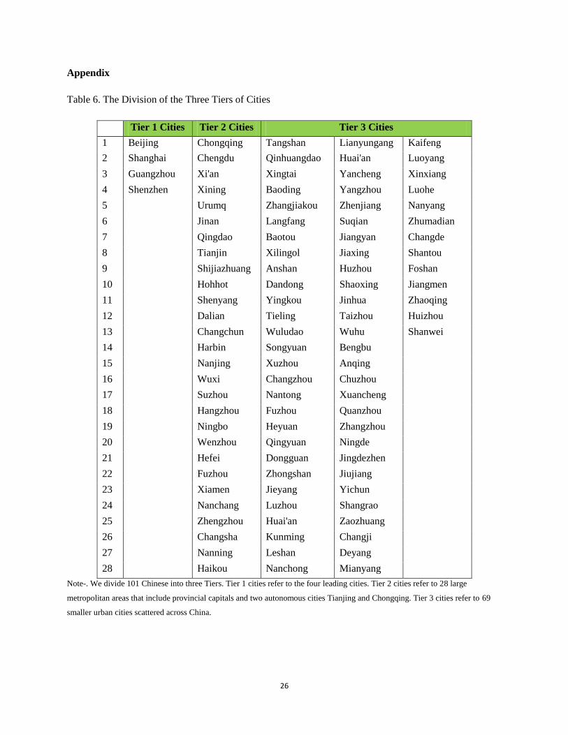
Appendix
Table 6. The Division of the Three Tiers of Cities
Tier 1 Cities
List
Tier 2 Cities Tier 3 Cities
Tier 3 Cities
Tier 3 Cities
1 Beijing Chongqing Tangshan Lianyungang Kaifeng
2 Shanghai Chengdu Qinhuangdao Huai'an Luoyang
3 Guangzhou Xi'an Xingtai Yancheng Xinxiang
4 Shenzhen Xining Baoding Yangzhou Luohe
5 Urumq Zhangjiakou Zhenjiang Nanyang
6 Jinan Langfang Suqian Zhumadian
7 Qingdao Baotou Jiangyan Changde
8 Tianjin Xilingol Jiaxing Shantou
9 Shijiazhuang Anshan Huzhou Foshan
10
Hohhot Dandong Shaoxing Jiangmen
11 Shenyang Yingkou Jinhua Zhaoqing
12 Dalian Tieling Taizhou Huizhou
13 Changchun Wuludao Wuhu Shanwei
14 Harbin Songyuan Bengbu
15 Nanjing Xuzhou Anqing
16 Wuxi Changzhou Chuzhou
17 Suzhou Nantong Xuancheng
18 Hangzhou Fuzhou Quanzhou
19 Ningbo Heyuan Zhangzhou
20 Wenzhou Qingyuan Ningde
21 Hefei Dongguan Jingdezhen
22 Fuzhou Zhongshan Jiujiang
23 Xiamen Jieyang Yichun
24 Nanchang Luzhou Shangrao
25 Zhengzhou Huai'an Zaozhuang
26 Changsha Kunming Changji
27 Nanning Leshan Deyang
28 Haikou Nanchong Mianyang
Note-. We divide 101 Chinese into three Tiers. Tier 1 cities refer to the four leading cities. Tier 2 cities refer to 28 large
metropolitan areas that include provincial capitals and two autonomous cities Tianjing and Chongqing. Tier 3 cities refer to 69
smaller urban cities scattered across China.