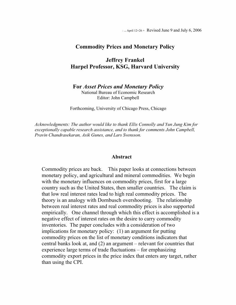
: +PEPI April 12+26 + Revised June 9 and July 6, 2006

Commodity Prices and Monetary Policy

Jeffrey Frankel Harpel Professor, KSG, Harvard University

For Asset Prices and Monetary Policy National Bureau of Economic Research

Editor: John Campbell

Forthcoming, University of Chicago Press, Chicago Acknowledgments: The author would like to thank Ellis Connolly and Yun Jung Kim for exceptionally capable research assistance, and to thank for comments John Campbell, Pravin Chandrasekaran, Asik Gunes, and Lars Svensson.

Abstract

Commodity prices are back. This paper looks at connections between monetary policy, and agricultural and mineral commodities. We begin with the monetary influences on commodity prices, first for a large country such as the United States, then smaller countries. The claim is that low real interest rates lead to high real commodity prices. The theory is an analogy with Dornbusch overshooting. The relationship between real interest rates and real commodity prices is also supported empirically. One channel through which this effect is accomplished is a negative effect of interest rates on the desire to carry commodity inventories. The paper concludes with a consideration of two implications for monetary policy: (1) an argument for putting commodity prices on the list of monetary conditions indicators that central banks look at, and (2) an argument – relevant for countries that experience large terms of trade fluctuations – for emphasizing commodity export prices in the price index that enters any target, rather than using the CPI.

Commodity Prices and Monetary Policy

I. Introduction

Commodity prices are back, with a vengeance. In the 1970s, macroeconomic discussions were dominated by the oil price shocks

and other rises in agricultural and mineral products that were thought to play a big role in the stagflation of that decade.1 In the early 1980s, any discussion of alternative monetary regimes was not complete without a consideration of the gold standard and proposals for other commodity-based standards.

Yet the topic of commodity prices fell out of favor in the late 1980s and the 1990s. Commodity prices generally declined during that period; it must be that declining commodity prices are not considered as interesting as rising prices. Nobody seemed to notice how many of the victims of emerging market crises in the 1990s were oil producers that were suffering, among other things, from low oil prices (Mexico, Indonesia, Russia) or others suffering from low agricultural prices (Brazil and Argentina). The favorable effect of low commodity prices on macroeconomic performance -- in the US in the 1990s – delivering lower inflation than had been thought possible at such high rates of growth and employment, was occasionally remarked. But it was not usually described as a favorable supply shock, the mirror image of the adverse supply shocks of the 1970s. It always received far less attention than the influence of other factors, such as the declining prices of semi-conductors and other information technology and communication equipment. Indeed, anyone who talked about sectors where the product was clunky and mundane as copper, crude petroleum and soy beans was considered behind the times. In Alan Greenspan’s phrase, GDP had gotten “lighter.” Agriculture and mining no longer constituted a large share of the New Economy, and did not matter much in an age dominated by ethereal digital communication, evanescent dotcoms, and externally outsourced services.

Now oil prices and many broader indices of commodity prices are again at or near

all-time highs in nominal terms (copper, platinum, nickel and zinc, for example, all hit record highs in 2006, in addition to crude oil), and are very high in real terms as well. As a result, commodities are once again hot. It turns out that mankind has to live in the physical world after all ! Still, the initial reaction in 2003-04 was relaxed, on several grounds: (1) Oil was no longer a large share of the economy, it was said; (2) Futures markets showed that the “spike” in prices was expected to be only temporary; and (3) Monetary policy need focus only on the core CPI inflation rate and can safely ignore the volatile food and energy component, unless or until it starts to get passed through into the core rate. But by 2005-2006, the increase in prices had gone far enough to receive

1 A small dissenting minority viewed the increases in prices of oil and other commodities in the 1970s as the result of overly expansionary US monetary policy, rather than as an exogenous inflationary supply shock (the result of the 1973 Arab oil embargo and the 1979 fall of the Shah of Iran). After all, was it just a coincidence that other commodity prices had gone up at the same time, or in the case of agricultural products, had actually preceded the oil shocks?

2

much more serious attention. This was especially true with regard to the perceived permanence of oil prices, largely because the futures price had gone from implying that the rise in the spot price was mostly temporary to implying that is mostly permanent.

Certain lessons of the past are well-remembered, such as the dangers of the Dutch Disease for countries undergoing a commodity export boom. But others have been forgotten, or were never properly absorbed.2

With regard to point (3), it is time to examine more carefully the claim that if an increase in energy or agricultural prices does not appear in the core CPI, then monetary policy can ignore it. The first half of the paper will argue that high real commodity prices can be a signal that monetary policy is loose. Thus they can be a useful monetary indicator (among many others).

The current fashion is inflation-targeting, by which is usually meant targeting the CPI.3 To be sure, the emphasis is on the core inflation rate “excluding the volatile food and energy sector.” The leadership of the Federal Reserve has indicated that the oil-shock component of recent inflation upticks should be ignored and accommodated. But just because agricultural and mineral product prices are volatile, does not mean that there is no useful information in them. The prices of gold and other minerals used to be considered useful leading indicators of inflationary expectations, precisely because they moved faster than the sluggish prices of manufactured goods and services. Nor does the volatility mean that excluding such products from the price index that guides monetary policy is necessarily the right thing to do.

In the first place, the “core CPI” is not a concept that is especially well understood among the general population. Thus the public will not necessarily be reassured when the central bank explains that they should not be worried about big increases in food and energy prices. Attempts to explain away high numbers for headline inflation make it sound like the authorities are granting themselves an ad hoc self-pardon – like a “dog ate my homework” excuse. This can undermine the public credibility of the central bank;

2 One point in passing. With regard to conventional wisdom (2), it is curious that so many economists and central bankers are ready to accept that the futures price of oil is an unbiased forecast of the future spot price. This proposition of course would follow from the two propositions that the futures price is an accurate measure of expectations (no risk premium) and that expectations are rational. Both halves of the joint hypothesis are open to question. Few familiar with the statistics of forward exchange rates claim that they are an unbiased predictor of the future spot exchange rate. Few familiar with the statistics of the interest rate term structure claim that the long-term interest rate contains an unbiased predictor of future short term interest rates. Why, then, should we think that the oil futures price is an unbiased predictor of the future spot price? So the backwardation (forward prices below spot) in oil prices in 2004 was not necessarily a reason to be complacent, and the flattening or contango (forward prices above spot) in 2005-06 was not necessarily a reason to worry. Nevertheless, the large increase in the slope of the futures yield curve during the period 2004-06, the same period that the Federal Reserve was steadily raising interest rates, is consistent with the theory of this paper (although the move to contango came rather sharply, in early April 2005, rather than gradually). The theory entails that the slope depends on the interest rate plus storage costs minus convenience yield, as noted in footnote 8 below. 3 Among many other references: Bernanke, et al (1999), Svensson (1995, 1999), and Truman (2003).

3

but credibility and transparency is the whole point of announcing an observable target in the first place. Thus targeting the core CPI may not buy as much credibility as targeting something more easily understood (even if with a wider band).

The many proponents of inflation targeting will argue that the regime, if properly instituted, makes clear from the beginning that it excludes volatile commodity prices, so that there is no loss in credibility. But, in the second place, let us ask should the inflation target exclude commodity prices ? They may be important, on terms of trade grounds, especially in smaller countries. Stabilizing the traded goods sector is itself an important goal in a world where balance of payments deficits can lead to financial crises, in which the previously declared currency regime is often one among many subsequent casualties. Recent oil price increases have also illustrated the necessity to take into account terms of trade shocks that come on the import side as well as the export side. What is wanted for intermediate target is a price index that is more easily understood by the public than the core CPI, and also more robust with respect to terms of trade shocks than the overall CPI. Candidates include a producer price index and an export price index.

It is a tenet of international economics textbooks that a desirable property of a currency regime is that the exchange rate be allowed to vary with terms of trade shocks: that the currency automatically depreciates when world prices of the import commodity go up (say, oil for the US or Switzerland, or wheat for Japan or Saudi Arabia), and that it automatically depreciates when world prices of the export commodity go down (say oil for Saudi Arabia and wheat for Canada). Yet CPI targeting does not have this property. To keep the headline inflation rate constant one must respond to a rise on world markets in the dollar price of imported oil by tightening monetary policy and appreciating the currency against the dollar enough to prevent the domestic price of the importable from rising. This response is the opposite from accommodating the adverse terms of trade shock, which would require a depreciation. It is true that the core inflation rate does not share this unfortunate property with the headline rate (unless the price increase comes in non-energy commodities like semi-conductors that are in the core). But the other half of terms of trade shocks are declines on world markets in the price of a country’s export commodity. Theory says that when the dollar price of oil goes down, Saudi Arabia or Norway ought to depreciate against the dollar. But inflation targeting – either the headline CPI variety or the core CPI variety -- does not allow this result. One would need to target a price index that specifically featured prominently the price of the exportable. The fundamental difficulty is that excluding the volatile food and energy components is not sufficient to accommodate the terms of trade, either if some imports lie outside those two sectors or if some exports lie within those two sectors.

Throughout this paper we will adopt the familiar assumption that all goods can be

divided into homogeneous agricultural and mineral commodities, on the one hand, and differentiated manufactured goods and services on the other hand, and that the key distinction is that prices of the former are perfectly flexible, so that their markets always clear, and that prices of the latter are sticky in the short run, so that their markets do not.4 The plan is to look at connections between commodities and monetary policy. We begin 4 For young readers, I will record that these distinctions were originally due to Arthur Okun (1975), who called the two sectors auction goods vs. customer goods.

4

with the monetary influences on commodity prices (first for a large country, then a small one). We conclude with a viewpoint based on reverse causality: the possible influence of commodity prices on monetary policy in a consideration of what price index should be used as a nominal anchor. Even if one is wedded to, say, a Taylor rule, the question of what price index should be used merits discussion. The author proposes an export price index (or producer price index) in place of the CPI. If one is enamored of a simpler price-targeting regime, then the proposal is to Peg the Export Price Index (PEPI) in place of targeting the CPI.

II. The Effect of Monetary Policy on Real Commodity Prices A central purpose of this paper is to assert the claim that monetary policy, as

reflected in real interest rates, is an important – and usually under-appreciated -- determinant of the real prices of oil and other mineral and agricultural products, while far from the only determinant.

1. Effect of US short-term real interest rates on real US commodity prices

The argument can be stated in an intuitive way that might appeal to practitioners, as follows. High interest rates reduce the demand for storable commodities, or increase the supply, through a variety of channels:

• by increasing the incentive for extraction today rather than tomorrow (think of the rates at which oil is pumped, zinc is mined, forests logged, or livestock herds culled)

• by decreasing firms' desire to carry inventories (think of oil inventories held in tanks) • by encouraging speculators to shift out of commodity contracts (especially spot

contracts), and into treasury bills.

All three mechanisms work to reduce the market price of commodities, as happened when real interest rates were high in the early 1980s. A decrease in real interest rates has the opposite effect, lowering the cost of carrying inventories, and raising commodity prices, as happened during 2002-2004. Call it part of the "carry trade."5

a. Theory: The overshooting model

The theoretical model can be summarized as follows. A monetary contraction temporarily raises the real interest rate, whether via a rise in the nominal interest rate, a fall in expected inflation, or both. Real commodity prices fall. How far? Until commodities are widely considered "undervalued" -- so undervalued that there is an expectation of future appreciation (together with other advantages of holding inventories,

5 "Why Are Oil and Metal Prices High? Don’t Forget Low Interest Rates," Jeffrey Frankel (published as "Real Interest Rates Cast a Shadow Over Oil," Financial Times, April 15, 2005.

5

namely the "convenience yield") that is sufficient to offset the higher interest rate (and other costs of carrying inventories: storage costs plus any risk premium). Only then, when expected returns are in balance, are firms willing to hold the inventories despite the high carrying cost. In the long run, the general price level adjusts to the change in the money supply. As a result, the real money supply, real interest rate, and real commodity price eventually return to where they were.

The theory is the same as Rudiger Dornbusch's (1976) famous theory of exchange rate overshooting, with the price of commodities substituted for the price of foreign exchange - and with convenience yield, minus storage costs, substituted for the foreign interest rate. The deep reason for the overshooting phenomenon is that prices for agricultural and mineral products adjust rapidly, while most other prices adjust slowly.6

The theory can be reduced to its simplest algebraic essence as a claimed relationship between the real interest rate and the spot price of a commodity relative to its expected long-run equilibrium price. This relationship can be derived from two simple assumptions. The first one governs expectations. Let

s ≡ the spot price,

s ≡ its long run equilibrium,

p ≡ the economy-wide price index,

q ≡ s-p, the real price of the commodity, and

q ≡ the long run equilibrium real price of the commodity,

all in log form. Market participants who observe the real price of the commodity today lying above or below its perceived long-run value, expect it in the future to regress back to equilibrium over time, at an annual rate that is proportionate to the gap:

E [ ∆ (s – p ) ] ≡ E[ ∆q] = - θ (q- q ) . (1)

Or E (∆s) = - θ (q- q ) + E(∆p). (2)

Following the classic Dornbusch overshooting paper, we begin by simply asserting the reasonableness of the form of expectations in these equations: a tendency to regress back toward long run equilibrium. But, as in that paper, it can be shown that regressive expectations are also rational expectations, under certain assumptions regarding the

6 Frankel (1984).

6

stickiness of other goods prices (manufactures and services) and certain restrictions on parameter values. 7

The second equation concerns the decision whether to hold the commodity for another period – either leaving it in the ground or on the trees or holding it in inventories – or to sell it at today’s price and deposit the proceeds in the bank to earn interest. The arbitrage condition is that the expected rate of return to these two alternative courses of action must be the same: E ∆s + c = i, (3)

where

c ≡ cy – sc – rp

cy ≡ convenience yield from holding the stock (e.g., the insurance value of having an assured supply of some critical input in the event of a disruption, or in the case of gold the psychic pleasure component)

sc ≡ storage costs (e.g., costs of security to prevent plundering by others, rental rate on oil tanks or oil tankers, etc.),

rp ≡ risk premium, which is positive if being long in commodities is risky, and

i ≡ the interest rate.8

Combine equations (2) and (3):

- θ (q- q ) + E(∆p) + c = i =>

q- q = - (1/θ) (i - E(∆p) – c) . (4)

Equation (4) says that the real price of the commodity (measured relative to its long-run equilibrium) is inversely proportional to the real interest rate (measured relative to a constant term that depends on convenience yield). When the real interest rate is high, as in the 1980s, money flows out of commodities, just as it flows out of foreign currencies, emerging markets, and other securities. Only when the prices of these alternative assets are perceived to lie sufficiently below their future equilibria will the arbitrage condition be met. Conversely, when the real interest rate is low, as in 2001-05, money flows into commodities, just as it flows into foreign currencies, emerging markets, and other securities. Only when the prices of these alternative assets are perceived to lie sufficiently above their future equilibria will the arbitrage condition be met.

7 Frankel (1986).

8 Parenthetically, if one is interested in the derivatives markets, the forward discount or slope of the futures curve, f-s in log terms, is given by i-cy+sc, or equivalently by E ∆s – rp.

7

b. The simplest test

One can imagine a number of ways of testing the theory.

One way of isolating the macroeconomic effects on commodity prices is to look at jumps in financial markets that occur in immediate response to government announcements that change perceptions of monetary policy, as was true of Fed money supply announcements in the early 1980s. Money announcements that caused interest rates to jump up would on average cause commodity prices to fall, and vice versa. The experiment is interesting, because news regarding supply disruptions and so forth is unlikely to have come out during the short time intervals in question.9

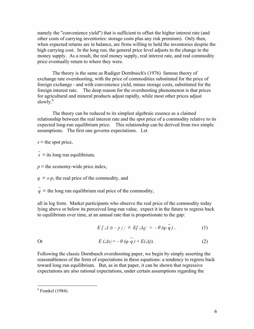
The relationship between the real commodity price and the real interest rate, equation (4), can also be tested more directly, because variables can be measured fairly easily.10 This is the test we pursue here. We begin with a look at some plots. Three major price indices that have been available since 1950 -- from Dow Jones, Commodity Resources Board, and Moody’s, are used in the first three figures. (In addition two others, which started later than 1950, are illustrated in an Appendix I ). To compute the real commodity price we take the log of the commodity price index minus the log of the CPI. To compute the real interest rate, we take the one-year interest rate and subtract off the one year inflation rate observed over the preceding year. The negative relationship predicted by the theory seems to hold. We next apply OLS regression to these data. We should not expect the relationship to hold precisely in practice. It would be foolish to think that the equation captures everything. In reality, a lot of other things beyond real interest rates influence commodity prices. There are bound to be fluctuations both in q , the long-run equilibrium real price, and c , which includes convenience yield, storage costs, and risk premium. These fluctuations are not readily measurable. Such factors as weather, political vicissitudes in producing countries, and so forth, are likely to be very important when looking at individual commodities. Indeed analysts of oil or coffee or copper pay rather little attention to macroeconomic influences, and instead spend their time looking at microeconomic determinants. Oil prices have been high in 2004-06 in large part due to booming demand from China and feared supply disruptions in the Middle East, Russia, Nigeria and Venezuela. There may now be a premium built in to the convenience yield arising from the possibilities of supply disruption related to terrorism, uncertainty in the Persian Gulf, and related risks. Yet another factor concerns the proposition that the world supply of oil may be peaking in this decade, as new discoveries lag behind consumption (Hubbert’s Peak11). This would

9 Frankel and Hardouvelis (1985).

10 One precedent: Barsky and Summers (1988, Part III) established an inverse relationship between the real interest rate and the real prices of gold and nonferrous metals. 11 Deffeyes (2005). Notwithstanding that such predictions have in the past been proven wrong.

8

imply that q , the world long run equilibrium real price of oil has shifted upward. Other factors apply to other commodities. In coffee, the large-scale entry of Vietnam into the market lowered prices sharply a few years ago. Corn, sugar, and cotton are heavily influenced by protectionist measures and subsidies in many countries. And so on.

Figure 1: US Real Commodity Prices and Real Interest Rates

Figure 1a

CRB Commodity Price Index vs. Real Interest Rate

Annual, 1950-2005

0.0

0.5

1.0

1.5

2.0

-7.5 -5.0 -2.5 0.0 2.5 5.0 7.5Real Interest Rate

Log

Rea

l Com

mod

ity P

rice

Inde

x

Source: Global Financial Data Inc.

9

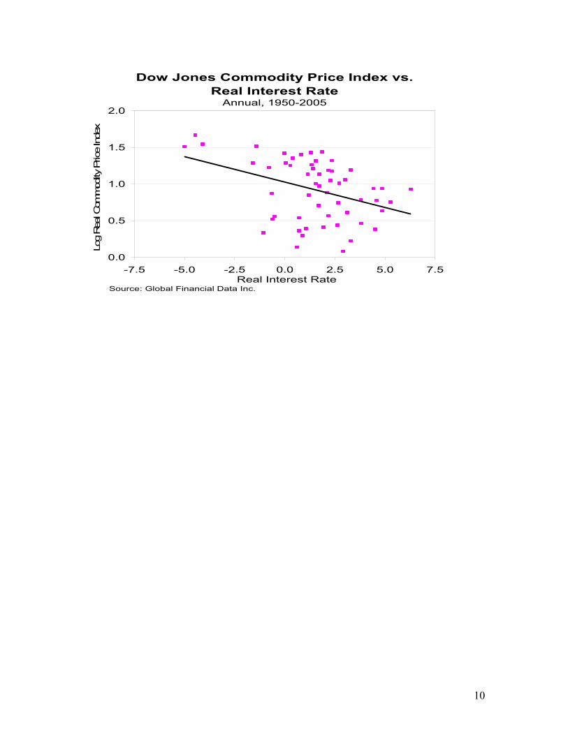
Dow Jones Commodity Price Index vs. Real Interest Rate

Annual, 1950-2005

0.0

0.5

1.0

1.5

2.0

-7.5 -5.0 -2.5 0.0 2.5 5.0 7.5Real Interest Rate

Log

Rea

l Com

mod

ity P

rice

Inde

x

Source: Global Financial Data Inc.

10

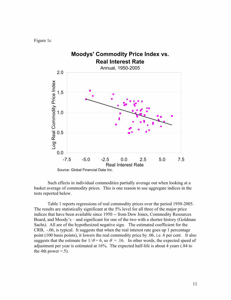
Figure 1c

Moodys' Commodity Price Index vs. Real Interest Rate

Annual, 1950-2005

0.0

0.5

1.0

1.5

2.0

-7.5 -5.0 -2.5 0.0 2.5 5.0 7.5Real Interest Rate

Log

Rea

l Com

mod

ity P

rice

Inde

x

Source: Global Financial Data Inc.

Such effects in individual commodities partially average out when looking at a basket average of commodity prices. This is one reason to use aggregate indices in the tests reported below.

Table 1 reports regressions of real commodity prices over the period 1950-2005. The results are statistically significant at the 5% level for all three of the major price indices that have been available since 1950 -- from Dow Jones, Commodity Resources Board, and Moody’s – and significant for one of the two with a shorter history (Goldman Sachs). All are of the hypothesized negative sign. The estimated coefficient for the CRB, -.06, is typical. It suggests that when the real interest rate goes up 1 percentage point (100 basis points), it lowers the real commodity price by .06, i.e. 6 per cent. It also suggests that the estimate for θ/1 = 6, so θ = .16. In other words, the expected speed of adjustment per year is estimated at 16%. The expected half-life is about 4 years (.84 to the 4th power =.5).

11

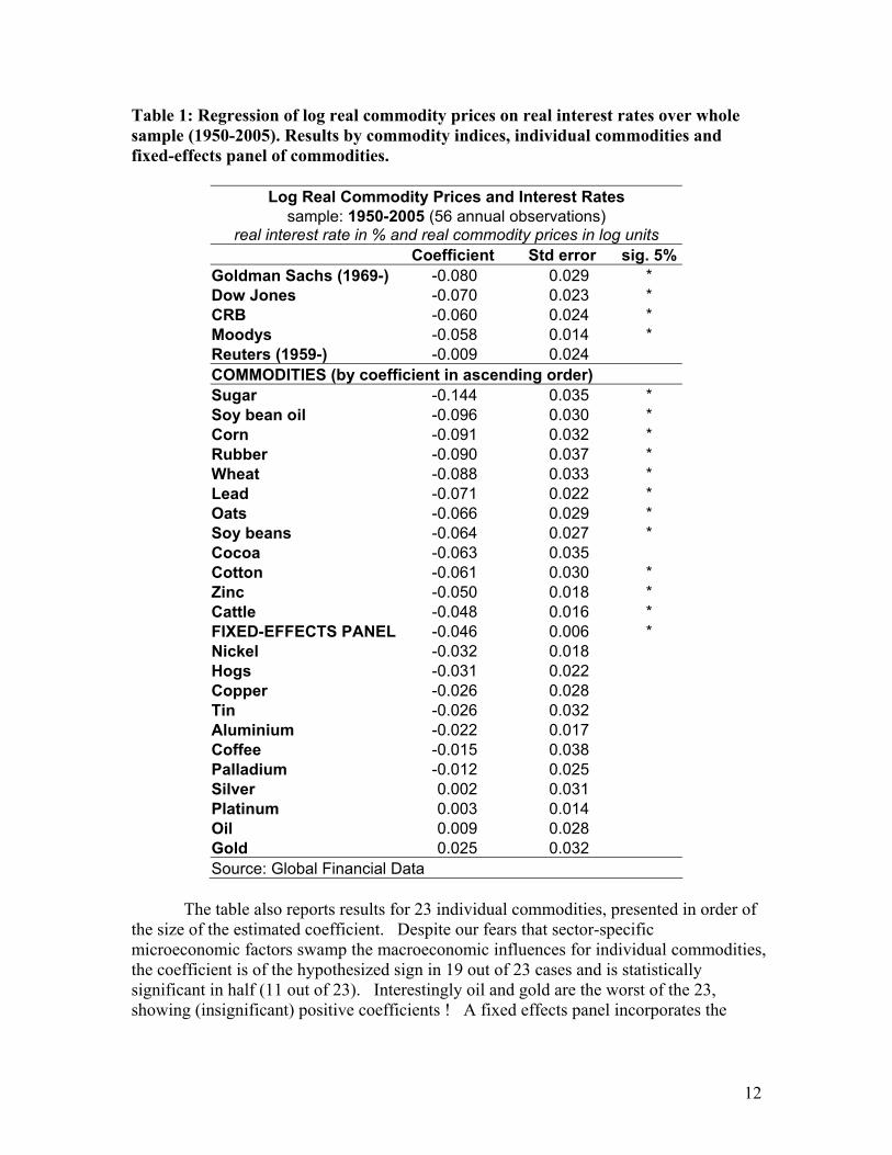
Table 1: Regression of log real commodity prices on real interest rates over whole sample (1950-2005). Results by commodity indices, individual commodities and fixed-effects panel of commodities.

Log Real Commodity Prices and Interest Rates sample: 1950-2005 (56 annual observations)

real interest rate in % and real commodity prices in log units Coefficient Std error sig. 5% Goldman Sachs (1969-) -0.080 0.029 * Dow Jones -0.070 0.023 * CRB -0.060 0.024 * Moodys -0.058 0.014 * Reuters (1959-) -0.009 0.024 COMMODITIES (by coefficient in ascending order) Sugar -0.144 0.035 * Soy bean oil -0.096 0.030 * Corn -0.091 0.032 * Rubber -0.090 0.037 * Wheat -0.088 0.033 * Lead -0.071 0.022 * Oats -0.066 0.029 * Soy beans -0.064 0.027 * Cocoa -0.063 0.035 Cotton -0.061 0.030 * Zinc -0.050 0.018 * Cattle -0.048 0.016 * FIXED-EFFECTS PANEL -0.046 0.006 * Nickel -0.032 0.018 Hogs -0.031 0.022 Copper -0.026 0.028 Tin -0.026 0.032 Aluminium -0.022 0.017 Coffee -0.015 0.038 Palladium -0.012 0.025 Silver 0.002 0.031 Platinum 0.003 0.014 Oil 0.009 0.028 Gold 0.025 0.032 Source: Global Financial Data

The table also reports results for 23 individual commodities, presented in order of the size of the estimated coefficient. Despite our fears that sector-specific microeconomic factors swamp the macroeconomic influences for individual commodities, the coefficient is of the hypothesized sign in 19 out of 23 cases and is statistically significant in half (11 out of 23). Interestingly oil and gold are the worst of the 23, showing (insignificant) positive coefficients ! A fixed effects panel incorporates the

12

information for all the individual commodities with the coefficient constrained to be the same. The coefficient is estimated at -.046 and is highly significant statistically.

The results in Table 1 suggest that the significant negative relationship between commodity prices and interest rates is reasonably robust across commodity price measures. Is the result is robust over time? It appears that the negative correlation is significant over 1950-1979 (Table 1a, reported in the appendix). However, since 1980, there does not appear to have been a stable relationship between log real commodity prices and the real interest rate (Table 1b). The same is true if the sample is divided at 1976 or 1982. c. An Effect on Inventories?

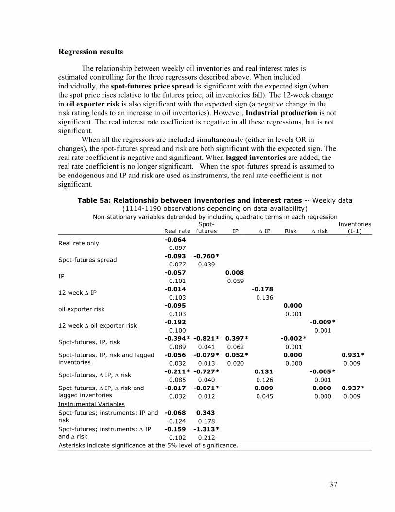
Since one of the hypothesized mechanisms of transmission from real interest rates to real commodity prices runs via the demand for inventories, it may be instructive to look at inventory data. Appendices 2 and 3 report regression results for oil inventories (Tables 4 and 5). The coefficient on the real interest rate is often negative, as hypothesized. It is not always statistically significant, until we control for three other standard determinants of inventory demand, as in Table 2 reported here. The three other determinants are:

• industrial production, representing the transactions demand for inventories • risk (political, financial, and economic) among a weighted average of 12 top

oil producers. • the spot-futures spread. Intuitively the spot-futures spread reflects the

convenience yield to holding inventories. 12 More formally, footnote 8 gives us the arbitrage condition relevant for firms deciding whether to incur storage costs:

i – cy + sc = E ∆s – rp

We substitute in the arbitrage condition that comes from the financial speculators,

f-s = E ∆s – rp , and solve for storage costs.

sc = f-s + cy - i

Storage costs rise with the extent to which inventory holdings strain existing storage capacity:

sc = Φ (INVENTORIES). Invert the equation for the supply of inventory storage capacity, and set inventory demand equal to supply:

INVENTORIES = Φ-1 ( sc ) = Φ-1 (cy - i – (s-f) )

We see from the equation that inventory holdings are positively related to convenience yield (which is in turn determined by industrial production and geopolitical risk), and negatively related

12 E.g., see the discussion of Figure 1.22 in the World Economic Outlook April 2006, International Monetary Fund, Washington, DC.

13

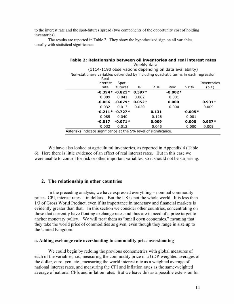
to the interest rate and the spot-futures spread (two components of the opportunity cost of holding inventories).

The results are reported in Table 2. They show the hypothesized sign on all variables, usually with statistical significance.

Table 2: Relationship between oil inventories and real interest rates -- Weekly data

(1114-1190 observations depending on data availability) Non-stationary variables detrended by including quadratic terms in each regression

Real interest

rate Spot-

futures IP ∆ IP Risk ∆ risk Inventories

(t-1) -0.394* -0.821* 0.397* -0.002*

0.089 0.041 0.062 0.001 -0.056 -0.079* 0.052* 0.000 0.931*

0.032 0.013 0.020 0.000 0.009

-0.211* -0.727* 0.131 -0.005*

0.085 0.040 0.126 0.001 -0.017 -0.071* 0.009 0.000 0.937*

0.032 0.012 0.045 0.000 0.009

Asterisks indicate significance at the 5% level of significance.

We have also looked at agricultural inventories, as reported in Appendix 4 (Table

6). Here there is little evidence of an effect of real interest rates. But in this case we were unable to control for risk or other important variables, so it should not be surprising.

2. The relationship in other countries

In the preceding analysis, we have expressed everything – nominal commodity prices, CPI, interest rates -- in dollars. But the US is not the whole world. It is less than 1/3 of Gross World Product, even if its importance in monetary and financial markets is evidently greater than that. In this section we consider other countries, concentrating on those that currently have floating exchange rates and thus are in need of a price target to anchor monetary policy. We will treat them as “small open economies,” meaning that they take the world price of commodities as given, even though they range in size up to the United Kingdom.

a. Adding exchange rate overshooting to commodity price overshooting

We could begin by redoing the previous econometrics with global measures of each of the variables, i.e., measuring the commodity price in a GDP-weighted averages of the dollar, euro, yen, etc., measuring the world interest rate as a weighted average of national interest rates, and measuring the CPI and inflation rates as the same-weighted average of national CPIs and inflation rates. But we leave this as a possible extension for

14

future research. Instead we take the US variables to be the global variables, and we proceed directly to look at small countries that by definition take the US/global variables as given.

The log spot price of the commodity in terms of currency j is given by s j = s ( j/$ ) + s ( $/c ), (5)

where s (j/$) is the spot exchange rate in units of currency j per $ and s($/c) is the spot price of commodity c in terms of $, what has hitherto been called simply s for the dollar case. The real exchange rate between currency j and the dollar is governed by the direct application of the Dornbusch overshooting model. (s(j/$) - s (j/$) ) - (pj - p j )+ (p$ - p $ ) = - (1/υ) (ij - i $ - [E(∆p j ) - E(∆p $ )] ). (6) Combining with equations (4) and (5), (s(j/c) - s (j/c) ) = (s(j/$) - s (j/$) ) + (s($/c) - s ($/c) )

= ( p j - p j ) - (1/υ) (ij - i$ - [E(∆p j ) - E(∆p $ )] ) - (1/θ) (i$ – E(∆p$) – c) .

(q(j/c) - q (j/c) )= - (1/υ)( rj -r$) - (1/θ) (r$ – c) . (7) where r$ is the US interest rate rj is the interest rate in country j .

Equation (7) says the real commodity price observed in country j will be high to the extent either that the local real interest rate is low relative to the US real rate, or to the extent that the US real interest rate is low. We tested this equation for 8 individual countries that currently have independently floating currencies (though they did not all have floating rates throughout the entire sample period).

We regressed the log of the real commodity price (converted to the currency of the small open economy and divided by the small open economy’s price level) on the two variables on the right-hand side of equation (7), the US real interest rate and the real interest differential between the small open economy and the US:

log ( )[ ] επβππβα +−+−−−+=• )()( 21

j/$USUSUSUSjj

j

USiii

PSCP .

The results for the 8 floating countries are reported in Tables 3a through 3f. The tables use 6 different commodity price indices: CRB, Dow Jones, The Economist, Goldman Sachs, Moody’s and Reuters. Monthly data were generally available for the developed countries from 1950. 13 To take full advantage of what data were available, the regressions were estimated separately for the 3-month interest rate (3 month Treasury notes or equivalent) and the long term interest rate with the largest sample (Australia: 10 year bond; Brazil: 30 year bond; Canada: 10+ year bond; Chile: 20 year bond; Mexico: 3 year bond; NZ: 10 year bond; Switzerland: 30 year bond; UK: 20 year bond). The US 13 For the three Latin American countries, however, it was difficult to find interest rate data preceding their hyperinflations.

15

interest rate for each regression was chosen to match the maturity of the bond from the small open economy.

16

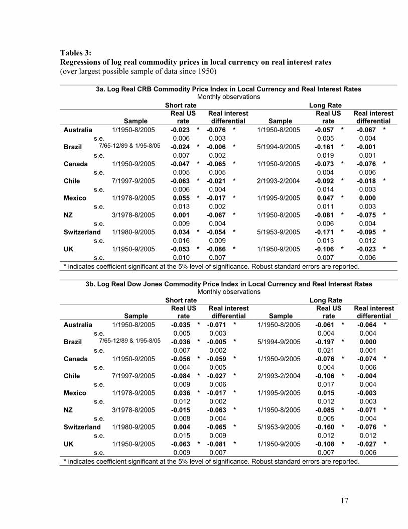
Tables 3: Regressions of log real commodity prices in local currency on real interest rates (over largest possible sample of data since 1950)

3a. Log Real CRB Commodity Price Index in Local Currency and Real Interest Rates Monthly observations

Short rate Long Rate

Sample Real US

rate Real interest differential Sample

Real US rate

Real interest differential

Australia 1/1950-8/2005 -0.023 * -0.076 * 1/1950-8/2005 -0.057 * -0.067 * s.e. 0.006 0.003 0.005 0.004

Brazil 7/65-12/89 & 1/95-8/05 -0.024 * -0.006 * 5/1994-9/2005 -0.161 * -0.001 s.e. 0.007 0.002 0.019 0.001

Canada 1/1950-9/2005 -0.047 * -0.065 * 1/1950-9/2005 -0.073 * -0.076 * s.e. 0.005 0.005 0.004 0.006

Chile 7/1997-9/2005 -0.063 * -0.021 * 2/1993-2/2004 -0.092 * -0.018 * s.e. 0.006 0.004 0.014 0.003

Mexico 1/1978-9/2005 0.055 * -0.017 * 1/1995-9/2005 0.047 * 0.000 s.e. 0.013 0.002 0.011 0.003

NZ 3/1978-8/2005 0.001 -0.067 * 1/1950-8/2005 -0.081 * -0.075 * s.e. 0.009 0.004 0.006 0.004

Switzerland 1/1980-9/2005 0.034 * -0.054 * 5/1953-9/2005 -0.171 * -0.095 * s.e. 0.016 0.009 0.013 0.012

UK 1/1950-9/2005 -0.053 * -0.086 * 1/1950-9/2005 -0.106 * -0.023 * s.e. 0.010 0.007 0.007 0.006

* indicates coefficient significant at the 5% level of significance. Robust standard errors are reported.

3b. Log Real Dow Jones Commodity Price Index in Local Currency and Real Interest Rates Monthly observations

Short rate Long Rate

Sample Real US

rate Real interest differential Sample

Real US rate

Real interest differential

Australia 1/1950-8/2005 -0.035 * -0.071 * 1/1950-8/2005 -0.061 * -0.064 * s.e. 0.005 0.003 0.004 0.004

Brazil 7/65-12/89 & 1/95-8/05 -0.036 * -0.005 * 5/1994-9/2005 -0.197 * 0.000 s.e. 0.007 0.002 0.021 0.001

Canada 1/1950-9/2005 -0.056 * -0.059 * 1/1950-9/2005 -0.076 * -0.074 * s.e. 0.004 0.005 0.004 0.006

Chile 7/1997-9/2005 -0.084 * -0.027 * 2/1993-2/2004 -0.106 * -0.004 s.e. 0.009 0.006 0.017 0.004

Mexico 1/1978-9/2005 0.036 * -0.017 * 1/1995-9/2005 0.015 -0.003 s.e. 0.012 0.002 0.012 0.003

NZ 3/1978-8/2005 -0.015 -0.063 * 1/1950-8/2005 -0.085 * -0.071 * s.e. 0.008 0.004 0.005 0.004

Switzerland 1/1980-9/2005 0.004 -0.065 * 5/1953-9/2005 -0.160 * -0.076 * s.e. 0.015 0.009 0.012 0.012

UK 1/1950-9/2005 -0.063 * -0.081 * 1/1950-9/2005 -0.108 * -0.027 * s.e. 0.009 0.007 0.007 0.006

* indicates coefficient significant at the 5% level of significance. Robust standard errors are reported.

17

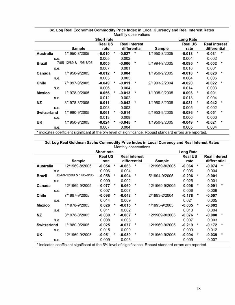
3c. Log Real Economist Commodity Price Index in Local Currency and Real Interest Rates Monthly observations

Short rate Long Rate

Sample Real US

rate Real interest differential Sample

Real US rate

Real interest differential

Australia 1/1950-8/2005 -0.010 * -0.027 * 1/1950-8/2005 -0.018 * -0.031 * s.e. 0.005 0.002 0.004 0.002

Brazil 7/65-12/89 & 1/95-8/05 0.005 -0.006 * 5/1994-9/2005 -0.095 * -0.002 * s.e. 0.007 0.001 0.018 0.001

Canada 1/1950-9/2005 -0.012 * 0.004 1/1950-9/2005 -0.018 * -0.020 * s.e. 0.005 0.005 0.004 0.006

Chile 7/1997-9/2005 -0.049 * -0.011 * 2/1993-2/2004 -0.020 -0.022 * s.e. 0.006 0.004 0.014 0.003

Mexico 1/1978-9/2005 0.056 * -0.013 * 1/1995-9/2005 0.093 * 0.001 s.e. 0.012 0.002 0.013 0.004

NZ 3/1978-8/2005 0.011 -0.042 * 1/1950-8/2005 -0.031 * -0.042 * s.e. 0.008 0.003 0.005 0.002

Switzerland 1/1980-9/2005 0.061 * -0.014 5/1953-9/2005 -0.086 * -0.051 * s.e. 0.013 0.008 0.006 0.006

UK 1/1950-9/2005 -0.024 * -0.045 * 1/1950-9/2005 -0.049 * -0.021 * s.e. 0.007 0.004 0.005 0.004

* indicates coefficient significant at the 5% level of significance. Robust standard errors are reported.

3d. Log Real Goldman Sachs Commodity Price Index in Local Currency and Real Interest Rates Monthly observations

Short rate Long Rate

Sample Real US

rate Real interest differential Sample

Real US rate

Real interest differential

Australia 12/1969-8/2005 -0.054 * -0.063 * 12/1969-8/2005 -0.064 * -0.074 * s.e. 0.006 0.004 0.005 0.004

Brazil 12/69-12/89 & 1/95-8/05 -0.058 * -0.004 * 5/1994-9/2005 -0.296 * -0.001 s.e. 0.009 0.002 0.025 0.001

Canada 12/1969-9/2005 -0.077 * -0.060 * 12/1969-9/2005 -0.096 * -0.091 * s.e. 0.007 0.007 0.006 0.006

Chile 7/1997-9/2005 -0.098 * -0.048 * 2/1993-2/2004 -0.178 * -0.007 s.e. 0.014 0.009 0.021 0.005

Mexico 1/1978-9/2005 0.026 * -0.015 * 1/1995-9/2005 -0.035 * -0.002 s.e. 0.011 0.002 0.013 0.004

NZ 3/1978-8/2005 -0.030 * -0.067 * 12/1969-8/2005 -0.076 * -0.080 * s.e. 0.008 0.003 0.007 0.003

Switzerland 1/1980-9/2005 -0.025 -0.077 * 12/1969-9/2005 -0.219 * -0.172 * s.e. 0.015 0.009 0.009 0.012

UK 12/1969-9/2005 -0.051 * -0.089 * 12/1969-9/2005 -0.094 * -0.039 * s.e. 0.009 0.005 0.009 0.007

* indicates coefficient significant at the 5% level of significance. Robust standard errors are reported.

18

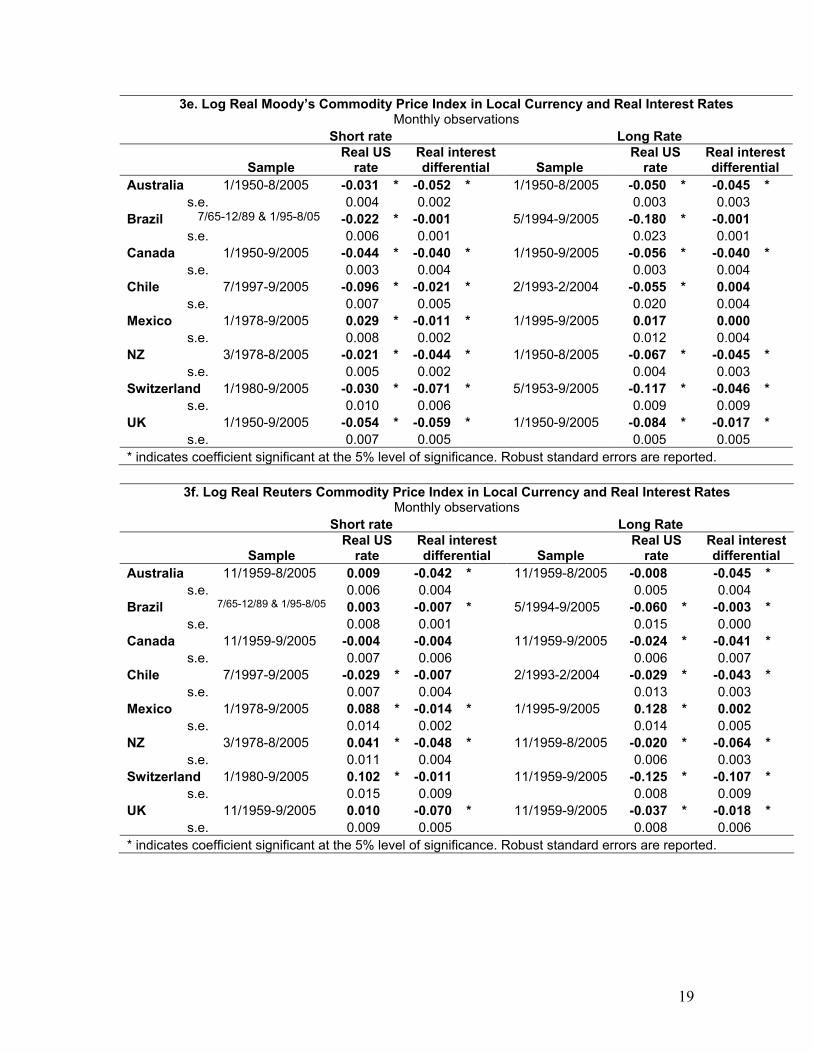
3e. Log Real Moody’s Commodity Price Index in Local Currency and Real Interest Rates Monthly observations

Short rate Long Rate

Sample Real US

rate Real interest differential Sample

Real US rate

Real interest differential

Australia 1/1950-8/2005 -0.031 * -0.052 * 1/1950-8/2005 -0.050 * -0.045 * s.e. 0.004 0.002 0.003 0.003

Brazil 7/65-12/89 & 1/95-8/05 -0.022 * -0.001 5/1994-9/2005 -0.180 * -0.001 s.e. 0.006 0.001 0.023 0.001

Canada 1/1950-9/2005 -0.044 * -0.040 * 1/1950-9/2005 -0.056 * -0.040 * s.e. 0.003 0.004 0.003 0.004

Chile 7/1997-9/2005 -0.096 * -0.021 * 2/1993-2/2004 -0.055 * 0.004 s.e. 0.007 0.005 0.020 0.004

Mexico 1/1978-9/2005 0.029 * -0.011 * 1/1995-9/2005 0.017 0.000 s.e. 0.008 0.002 0.012 0.004

NZ 3/1978-8/2005 -0.021 * -0.044 * 1/1950-8/2005 -0.067 * -0.045 * s.e. 0.005 0.002 0.004 0.003

Switzerland 1/1980-9/2005 -0.030 * -0.071 * 5/1953-9/2005 -0.117 * -0.046 * s.e. 0.010 0.006 0.009 0.009

UK 1/1950-9/2005 -0.054 * -0.059 * 1/1950-9/2005 -0.084 * -0.017 * s.e. 0.007 0.005 0.005 0.005

* indicates coefficient significant at the 5% level of significance. Robust standard errors are reported.

3f. Log Real Reuters Commodity Price Index in Local Currency and Real Interest Rates Monthly observations

Short rate Long Rate

Sample Real US

rate Real interest differential Sample

Real US rate

Real interest differential

Australia 11/1959-8/2005 0.009 -0.042 * 11/1959-8/2005 -0.008 -0.045 * s.e. 0.006 0.004 0.005 0.004

Brazil 7/65-12/89 & 1/95-8/05 0.003 -0.007 * 5/1994-9/2005 -0.060 * -0.003 * s.e. 0.008 0.001 0.015 0.000

Canada 11/1959-9/2005 -0.004 -0.004 11/1959-9/2005 -0.024 * -0.041 * s.e. 0.007 0.006 0.006 0.007

Chile 7/1997-9/2005 -0.029 * -0.007 2/1993-2/2004 -0.029 * -0.043 * s.e. 0.007 0.004 0.013 0.003

Mexico 1/1978-9/2005 0.088 * -0.014 * 1/1995-9/2005 0.128 * 0.002 s.e. 0.014 0.002 0.014 0.005

NZ 3/1978-8/2005 0.041 * -0.048 * 11/1959-8/2005 -0.020 * -0.064 * s.e. 0.011 0.004 0.006 0.003

Switzerland 1/1980-9/2005 0.102 * -0.011 11/1959-9/2005 -0.125 * -0.107 * s.e. 0.015 0.009 0.008 0.009

UK 11/1959-9/2005 0.010 -0.070 * 11/1959-9/2005 -0.037 * -0.018 * s.e. 0.009 0.005 0.008 0.006

* indicates coefficient significant at the 5% level of significance. Robust standard errors are reported.

19

In general, the evidence appears to support the hypothesis regarding the determination the log real local-currency index of commodity prices. The estimates show a significant negative coefficient on the real US interest rate, representing global monetary policy, as well as on the real interest differential between the national economy and the US, representing local variations in monetary stance. Often significance levels are high. In the case of the three major English-speaking countries, Australia, Canada and the United Kingdom, both the coefficient on the US real interest rate and the coefficient on the real interest differential are statistically significant and of the hypothesized negative sign in almost every one of the 12 cases, regardless which of the 6 commodity price indices are used and regardless whether short-term or long-term interest rates are used. The results for New Zealand and Switzerland are almost as strong but for the effect of the short-term US rate; as are the results for Brazil and Chile, except that the coefficient on the long-term real interest differential is not always significant. The only disappointing country is Mexico, where even though the short-term real interest differential always appears significantly less than zero, the US interest rate appears significantly greater than zero rather than less. This seems impressive evidence for what has been the central theme of this paper so far. The hypothesized effect of the real interest rate on real commodity prices works not only at the US level, but also at the level of local variation among open economies above and beyond the global phenomenon.

III. Implications for Monetary Policy

We conclude the paper with a consideration of some implications for monetary policy makers. The first implication is an argument for adding commodity prices to the list of variables that central banks monitor, regardless what is their regime– i.e., regardless whether they use discretion or some rule or intermediate target, and in the latter case regardless what is the rule or target that is officially declared. The second implication is an argument, in the case of countries where fluctuations in the terms of trade are important, for giving export prices a larger role in the price index that enters the rule or target than does the CPI (whether headline CPI or core CPI). 1. Commodity Prices Belong on the List of Monetary Conditions Indicators

To say that monetary policy makers should “look at everything” is advice that

sounds easy to give and hard to reject. But not everyone would consider it obvious that an index of agricultural and mineral commodity prices belongs on a useful list of variables that are thought to reveal current monetary conditions, alongside short and long-term interest rates, the exchange rate, housing prices, and the stock market. The conventional wisdom is that the volatile “food and energy” sector should be thrown out of the price indices, and that one should concentrate of the core CPI if one wants a good indicator of likely future inflation. It is certainly true that if one is looking for the single standard statistic that best predicts future inflation, the core CPI will do better than the headline CPI. But that is not the question. The question is, rather, if one is free to look at lots of information, are agricultural and mineral prices on the list of variables worth

20

paying attention to. This perspective places this chapter on a plane with other chapters asking whether central banks should pay attention to housing prices or the stock market.

My answer would be “yes.” The theory and empirical results presented in the paper support the claim that real commodity prices reflect real interest rates, among other factors. We can never be sure what the real interest rate is, because we do not directly observe expected inflation. Thus it is useful to have additional data that are thought to reflect real interest rates.

2. What Prices Should Inflation Targeters Target?

The current fashion in monetary policy regimes is inflation targeting. Such countries as the United Kingdom, Sweden, Canada, New Zealand, Australia, Chile, Brazil, Norway, Korea, and South Africa have adopted it, and many monetary economists approve. In part this is a consequence of the disillusionment with exchange rate targets that arose in the course of ten years of currency crises (from the speculative attack that forced the UK to drop out of the European Exchange Rate Mechanism in 1992 to the Argentina crisis of 2001). Proponents of inflation targeting point out that if the exchange rate is not to be the anchor for monetary policy, then the ultimate objective of price stability requires that some new nominal variable must be chosen as the anchor. Two old favorite candidates for nominal anchor, the price of gold and the money supply, have long since been discredited in the eyes of many. So that seems to leave inflation targeting. One version of a generalized approach to inflation targeting is a Taylor rule, which puts weight on output in addition to inflation. But whether it is simple inflation targeting or a Taylor rule, what price index should be used? Of the possible price indices that a central bank could target, the CPI is the usual choice. Indeed the CPI (whether core or overall CPI) seems to be virtually the only choice that central banks and economists have even considered. But this may not be the best choice. I want to argue for targeting an index of export prices. 3. The Proposal to Peg the Export Price (PEP) This idea is a more moderate version of an exotic-sounding proposed monetary regime that I have written about elsewhere, called Peg the Export Price – or PEP, for short. I have proposed PEP explicitly for those countries that happen to be heavily specialized in the production of a particular mineral or agricultural export commodity. The proposal is to fix the price of that commodity in terms of domestic currency, or, equivalently, set the value of domestic currency in terms of that commodity. For example, African gold producers would peg their currency to gold – in effect returning to the long-abandoned gold standard. Canada and Australia would peg to wheat. Norway would peg to oil. Chile would peg to copper, and so forth. One can even think of exporters of manufactured goods that qualify: standardized semi-conductors (that is, commodity chips) are sufficiently important exports in Korea that one could imagine it pegging the won to the price of chips.

How would this work operationally? Conceptually, one can imagine the government holding reserves of gold or oil, and intervening whenever necessary to keep the price fixed in terms of local currency. Operationally, a more practical method would

21

be for the central bank each day to announce an exchange rate vis-à-vis the dollar, following the rule that the day’s exchange rate target (dollars per local currency unit) moves precisely in proportion to the day’s price of gold or oil on the London market or New York market (dollars per commodity). Then the central bank could intervene via the foreign exchange market to achieve the day’s target. Either way, the effect would be to stabilize the price of the commodity in terms of local currency. Or perhaps, since these commodity prices are determined on world markets, a better way to express the same policy is “stabilizing the price of local currency in terms of the commodity.”14

The PEP proposal can be made more moderate, and more appropriate for diversified economies, in a number of ways.15 One is to interpret it as targeting a broad index of all export prices, rather than the price of only one or a few export commodities. This moderate form of the proposal is abbreviated PEPI, for Peg the Export Price Index.16 The argument for the export price targeting proposal, in any of its forms, can be stated succinctly: It delivers one of the main advantages that a simple exchange rate peg promises, namely a nominal anchor, while simultaneously delivering one of the main advantages that a floating regime promises, namely automatic adjustment in the face of fluctuations in the prices of the countries’ exports on world markets. Textbook theory says that when there is an adverse movement in the terms of trade, it is desirable to accommodate it via a depreciation of the currency. When the dollar price of exports rises, under PEP or PEPI the currency per force appreciates in terms of dollars. When the dollar price of exports falls, the currency depreciates in terms of dollars. Such accommodation of terms of trade shocks is precisely what is wanted. In recent currency crises, countries that suffered a sharp deterioration in their export markets were often eventually forced to give up their exchange rate targets and devalue anyway; but the adjustment was far more painful -- in terms of lost reserves, lost credibility, and lost output -- than if the depreciation had happened automatically. But the proposal is not just for countries with volatile commodity exports. The desirability of accommodating terms of trade shocks is a particularly good way to summarize the attractiveness of export price targeting relative to the reigning champion, CPI targeting. 17 Consider the two categories of adverse terms of trade shocks: a fall in the dollar price of the export in world markets and a rise in the dollar price of the import on world markets. In the first case, a fall in the export price, you want the local currency to depreciate against the dollar. As already noted, PEP or PEPI deliver that result automatically; CPI targeting does not. In the second case, a rise in the import price, the

14 Frankel (2002, 2003) and Frankel and Saiki (2002). 15 One possible margin of moderation is the width of the band: one can define a broad band as a target around the central parity, rather than seeking to fix the price perfectly. Another way to go is to define as the parity a basket that includes the export commodity as well as a weighted average of currencies of major trading partners – e.g., 1/3 dollars, 1/3 euros, and 1/3 oil, as the author has proposed for Persian Gulf states. 16 Frankel (2005). 17 Among many possible references are Bernanke, et al. (1999), Mankiw and Reis (2003), Svensson (1995, 1999), Svennson and Woodward (2005), and Truman (2003).

22

terms-of-trade criterion suggests that you again want the local currency to depreciate.18 CPI targeting actually has the implication that you tighten monetary policy so as to appreciate the currency against the dollar, by enough to prevent the local-currency price of imports from rising. This implication – reacting to an adverse terms of trade shock by appreciating the currency – seems perverse. It could be expected to exacerbate swings in the trade balance, and output.

Few believe that the proper response for an oil-importing country in the event of a large increase in world oil prices is to tighten monetary policy and thereby appreciate the currency sufficiently to prevent an increase in the price of oil in terms of domestic currency. The usual defense of inflation targeting offered by its many proponents is that in the event of such a shock, the central bank should deviate from the CPI target and explain the circumstances to the public. But what can be the argument for making such derogations on an ad hoc basis, when it is possible to build them into a simple target rule in the first place? Certainly not a gain in transparency and credibility. CPI targeting is not unique in having an Achilles heel, in the form of import price shocks. Other standard candidates for nominal anchor have their own problems. 4. Each Candidate for Nominal Anchor has its Own Vulnerability

Each of the variables that are candidates for nominal anchor has its own characteristic sort of extraneous fluctuations that can wreck havoc on a country’s monetary system.

• A monetarist rule would specify a fixed rate of growth in the money supply. But

fluctuations in the public’s demand for money or in the behavior of the banking system can directly produce gratuitous fluctuations in velocity and the interest rate, and thereby in the real economy. For example, in the United States, a large upward shift in the demand for money around 1982 convinced the Federal Reserve Board that it had better abandon the money growth rule it had adopted two years earlier, or else face a prolonged and severe recession.

• Under a gold standard, the economy is hostage to the vagaries of the world gold

market. For example, when much of the world was on the gold standard in the 19th century, global monetary conditions depended on the output of the world’s gold mines. The California gold rush from 1849 was associated with a mid-century increase in liquidity and a resulting increase in the global price level. The absence of major discoveries of gold between 1873 and 1896 helps explain why price levels fell dramatically over this period. In the late 1890s, the gold rushes in Alaska and South Africa were each again followed by new upswings in the price level. Thus the system did not in fact guarantee stability.19

18 Neither regime delivers that result. There is a reason for this. In addition to the goal of accommodating terms of trade shocks, there is also the goal of resisting inflation; but to depreciate in the face of an increase in import prices would exacerbate price instability. 19 Cooper (1985). On the classical gold standard, see also papers in Eichengreen (1985).

23

• One proposal is that monetary policy should target a basket of basic mineral and agricultural commodities. The idea is that a broad-based commodity standard of this sort would not be subject to the vicissitudes of a single commodity such as gold, because fluctuations of its components would average out somewhat.20 The proposal might work if the basket reflected the commodities produced and exported by the country in question. But for a country that is a net importer of oil, wheat, and other mineral and agricultural commodities, such a peg gives precisely the wrong answer in a year when the prices of these import commodities go up. Just when the domestic currency should be depreciating to accommodate an adverse movement in the terms of trade, it appreciates instead. Switzerland should not peg to oil, and Norway should not peg to wheat.

• The need for robustness with respect to import price shocks argues for the superiority

of nominal income targeting over inflation targeting.21 A practical argument against nominal income targeting is the difficulty of timely measurement, and subsequent revisions.

• Under a fixed exchange rate, fluctuations in the value of the particular currency to

which the home country is pegged can produce needless volatility in the country’s international price competitiveness. For example, the appreciation of the dollar from 1995 and 2001 was also an appreciation for whatever currencies were linked to the dollar. Regardless the extent to which one considers the late-1990s dollar appreciation to have been based in the fundamentals of the US economy, there was no necessary connection to the fundamentals of smaller dollar-linked economies. The problem was particularly severe for some far-flung economies that had adopted currency boards over the preceding decade: Hong Kong, Argentina, and Lithuania.

• This brings us back to the current fashion of targeting the inflation rate or CPI. To

some, PEP may sound similar to inflation targeting. But, as already noted, a key difference between the CPI and the export price is the terms of trade. When there is an adverse movement in the terms of trade, one would like the currency to depreciate, while price level targeting can have the opposite implication. If the central bank has been constrained to hit an inflation target, oil price shocks (as in 1973-74, 1979-80, and 2000-06), for example, will require an oil-importing country to tighten monetary policy. The result can be sharp falls in national output. Thus under rigid inflation targeting, supply or terms-of-trade shocks can produce unnecessary and excessive fluctuations in the level of economic activity.

20 A “commodity standard” was proposed in the 1930s – by B. Graham (1937) – and subsequently discussed by Keynes (1938), and others. It was revived in the 1980s: e.g., Hall (1982). 21 Velocity shocks argue for the superiority of nominal income targeting over a monetarist rule. Frankel (1995) demonstrates the point mathematically, using the framework of Rogoff (1985), and gives other references on nominal income targeting.

24

Among a set of major countries who today target inflation, there is a positive correlation between between changes in import prices on world markets (expressed in dollars/import), and changes in the exchange rate (expressed in dollars/local currency). . In other words these countries respond to increases in world prices of their imports by appreciating their currencies rather than depreciating them. This is consistent with CPI-targeting, but seems to fly in the face of the textbook principle of floating exchange rates that a country’s monetary policy should respond to an adverse shift in the terms of trade so as to depreciate the currency rather than appreciate it.22

Consider the recent history. Australia, Canada, New Zealand, Singapore, Sweden, Switzerland, and the UK each after 2002 experienced increases in the prices of their imports on world markets, expressed in dollars. The textbook theory says that their currencies should have been allowed to depreciate to accommodate this adverse shift in their terms of trade, to give resources the incentive to shift out of the production of importables. But this did not happen. In each case, one could say that monetary policy was sufficiently tight, relative to the United States, that their currencies appreciated against the dollar. In each case, the observable result was that an index of import prices in local currency did not rise, but if anything actually fell. Why? Inflation-targeting is the obvious culprit. The implication is that this regime obligated them to tighten sufficiently to prevent a large increase in local currency import prices and therefore in the CPI.23

By contrast, in 1974 and 1980, large increases in these countries’ import prices on world markets were reflected as large increases in domestic currency import prices as well. This was before these countries switched to inflation targeting.

To recap, each of the most popular variables that have been proposed as candidates for nominal anchors is subject to fluctuations that will add an element of unnecessary monetary volatility to a country that has pegged its money to that variable: velocity shocks in the case of M1, supply shocks in the case of inflation targeting, measurement errors in the case of nominal GDP targeting, fluctuations in world gold markets in the case of the gold standard, and fluctuations in the anchor currency in the case of exchange rate pegs. PEPI does not have these vulnerabilities.

The argument for PEPI over CPI targeting is two-fold. First, as just demonstrated, CPI targeting requires tightening in the face of an increase in the world price of import commodities, such as oil for an oil importer, while PEPI does not. Second, PEPI allows accommodation of fluctuations in the world price of the export commodities, while CPI targeting does not. 5. Peg the Export Price Index

The second of the two arguments for the PEPI proposal just given is to eliminate export price variability. 24 The stability in export prices, in turn, would help stabilize the 22 See Frankel (2005, Table 2 and Figure 1). 23 Presumably the import price indices in terms of dollars rose in 2003 not just because of tight world markets for oil and other commodities, but also because of the depreciating dollar. 24 This is half the argument. Recall that the other half of the argument for PEPI, as compared to CPI targeting, is that it does not require tightening in the face of increases in the world price of imports.

25

balance of payments. It would, for example, have allowed the Korean won to depreciate automatically in the late 1990s, without the need for a costly failed attempt to defend an exchange rate target before the devaluation.25 It would have allowed the Malaysian ringgit to appreciate automatically in the early 2000s, without the need for the monetary authorities to abandon their nominal anchor, as they did in 2005. How would PEPI be implemented operationally? That is, how would an index of export prices be stabilized? As noted at the outset, in the simple version of the PEP proposal, there is nothing to prevent a central bank from intervening to fix the price of a single agricultural or mineral product perfectly on a day-to-day basis. Such perfect price fixing is not possible in the case of a broad basket of exports, as called for by PEPI, even if it were desirable. For one thing, such price indices are not even computed on a daily basis. So it would be, rather, a matter of setting a target zone for the year, with monthly realizations, much as a range for the CPI is declared under the most standard interpretation of inflation targeting.

The declared band could be wide if desired, just as with the targeting of the CPI, money supply, exchange rate, or other nominal variables. Open market operations to keep the export price index inside the band if it threatens to stray outside could be conducted in terms either of foreign exchange or in terms of domestic securities. For some countries, it might help to monitor on a daily or weekly basis the price of a basket of agricultural and mineral commodities that is as highly correlated as possible with the country’s overall price index, but whose components are observable on a daily or weekly basis in well-organized markets. The central bank could even announce what the value of the basket index would be one week at a time, by analogy with the Fed funds target in the United States. The weekly targets could be set so as to achieve the medium-term goal of keeping the comprehensive price index inside the pre-announced bands; and yet the central bank could hit the weekly targets very closely, if it wanted, for example, by intervening in the foreign exchange market.

A first step for any central bank wishing to dip its toe in these waters would be to compute a monthly index of export prices and publish it. A second step would be to announce that it was “monitoring” the index. The data requirements for computing such an index would not be great. Every country’s customs services gathers data on trade volumes and prices; indeed they tend to do so at earlier stages of development than they gather data on national income or the CPI. For countries that lack fully credible institutions, an added advantage of the PEP proposal is transparency: the components tend to be more readily observable than components of the CPI such as prices of housing or other nontraded services.

A still more moderate, still less exotic-sounding, version of the PEPI proposal would be to target a producer price index (PPI). In practice, it can be difficult to separate production cleanly into the two sectors, nontraded goods and exportables, in which case

25 Earlier research reported simulations of the path of exports over the last three decades if countries had followed the PEP proposal, as compared to hypothetical rigid pegs to a major currency, or as compared to whatever policy the country in fact followed historically: Frankel (2002) focuses primarily on producers of gold, Frankel (2003) on oil exporters, and Frankel and Saiki (2002) on various other agricultural and mineral producers. A typical finding was that developing countries that suffered a deterioration in export markets in the late 1990s, often contributing to a financial crisis, would have adjusted automatically under the PEP regime.

26

the two versions of the proposal – targeting an export price index or a producer price index -- come down to the same thing. The key point of the PEP proposal is to exclude import prices from the index, and to include export prices (as the PPI also does). The problem with CPI targeting is that it does it the other way around. References Abosedra, Salah; Radchenko, Stanislav (2003), "Oil Stock Management and Futures Prices: An Empirical Analysis", Journal of Energy and Development, vol. 28, no. 2, Spring 2003, pp. 173-88 Balabanoff, Stefan (1995), "Oil Futures Prices and Stock Management: A Cointegration Analysis", Energy Economics, vol. 17, no. 3, July 1995, pp.205-10. Barsky, Robert, and Lawrence Summers (1988) “Gibson’s Paradox and the Gold Standard,” Journal of Political Economy, 96, no. 3, 528-550. Bernanke, Ben, Thomas Laubach, Frederic Mishkin, and Adam Posen (1999), Inflation Targeting: Lessons from the International Experience, Princeton University Press: Princeton NJ, 1999. Bordo, Michael, and Anna J. Schwartz (1996), “The Specie Standard as a Contingent Rule: Some Evidence for Core and Peripheral Countries, 1880-1990” in Currency Convertibility: The Gold Standard and Beyond, J. Braga de Macedo, B. Eichengreen, J. Reis, eds., pp. 11-83 (New York: Routledge). Cooper, Richard (1985), “The Gold Standard: Historical Facts and Future Prospects” Brookings Papers on Economic Activity, 1, 1-45. Deffeyes, Kenneth (2005) Beyond Oil: The View from Hubbert’s Peak (Hill and Wang). Dornbusch, Rudiger (1976) "Expectations and Exchange Rate Dynamics" Journal of Political Economy 84, 1161-1176. Edwards, Sebastian (2002), “The Great Exchange Rate Debate After Argentina,” NBER Working Paper No. 9257, October. Edwards, Sebastian and Eduardo Levy Yeyati (2003), “Flexible Exchange Rates as Shock Absorbers,” NBER Working Paper No. 9867, July. Eichengreen, Barry (1985), The Gold Standard in Theory and History. New York, Methuen.

27

Frankel, Jeffrey, "Expectations and Commodity Price Dynamics: The Overshooting Model," Amer. J. of Agric. Ec. 68, no. 2 (1986), 344-348. Reprinted in Frankel, Financial Markets and Monetary Policy, MIT Press, 1995. _____ "Commodity Prices and Money: Lessons from International Finance," American J. of Agr. Economics 66, no. 5 (1984), 560-566. _____ (1995), "The Stabilizing Properties of a Nominal GNP Rule," Journal of Money, Credit and Banking 27, no. 2, May, 318-334. ______ "Should Gold-Exporters Peg Their Currencies to Gold?" Research Study No. 29, World Gold Council, London, UK, 2002. ______"A Proposed Monetary Regime for Small Commodity-Exporters: Peg the Export Price (‘PEP’)," International Finance (Blackwill Publ.), vol. 6, no. 1, Spring 2003, 61-88. ________ “Peg the Export Price Index: A Proposed Monetary Regime for Small Countries,” vol. 27, no. 4, June 2005, J. of Policy Modeling . Frankel, Jeffrey and Gikas Hardouvelis: "Commodity Prices, Money Surprises, and Fed Credibility," Journal of Money, Credit and Banking 17, no. 4 (Nov. 1985, Part I), 427-438. Reprinted in Frankel op cit. Frankel, Jeffrey, and Ayako Saiki, "A Proposal to Anchor Monetary Policy by the Price of the Export Commodity" Journal of Economic Integration, Sept. 2002, Vol. 17, No. 3, 417-448. Graham, Benjamin (1937), Storage and Stability. New York: McGraw Hill. Hall, Robert (1982), “Explorations in the Gold Standard and Related Policies for Stabilizing the Dollar,” in Hall, ed., Inflation. Chicago: Univ. of Chicago Press, 111-122. Keynes, John Maynard (1938), “The Policy of Government Storage of Foodstuffs and Raw Materials,” Economic Journal, September. Mankiw, N. Gregory, and Ricardo Reis (2003), “What Measure of Inflation Should a Central Bank Target?” in Lars Svensson and James Stock, editors, International Seminar on Macroeconomics, in Journal of the European Economic Association, 1, no. 5, September, The MIT Press, Cambridge . Okun, Arthur (1975).” Inflation: Its Mechanics and Welfare Costs.” Brookings Papers on Economic Activity 2: 351-401. Rogoff, Kenneth (1985),. “The Optimal Degree of Commitment to an Intermediate Monetary Target,” Quarterly Journal of Economics 100 (November): 1169-89.

28

Svensson, Lars (1995), “The Swedish Experience of an Inflation Target,” in Inflation Targets, edited by Leo Leiderman and Lars Svensson. Centre for Economic Policy Research, London.

-------- (1999), "Inflation Targeting as a Monetary Policy Rule," Journal of Monetary Economics 43: 607-654.

Svensson, Lars, and Michael Woodford (2005), “ Implementing Optimal Policy through Inflation-Forecast Targeting," in Ben Bernanke and Michael Woodford, eds., The Inflation-Targeting Debate, University of Chicago Press, Chicago,

Truman, Edwin (2003) Inflation Targeting in the World Economy, Institute for International Economics, Washington DC.

29

(amalgamated 2 Oct. 2005; revised and extended April 2006)

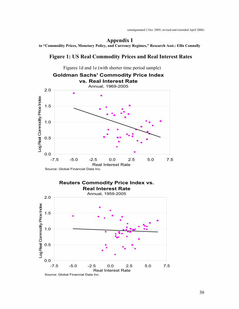
Appendix I to “Commodity Prices, Monetary Policy, and Currency Regimes,” Research Asst.: Ellis Connolly

Figure 1: US Real Commodity Prices and Real Interest Rates

Figures 1d and 1e (with shorter time period sample) Goldman Sachs' Commodity Price Index

vs. Real Interest RateAnnual, 1969-2005

0.0

0.5

1.0

1.5

2.0

-7.5 -5.0 -2.5 0.0 2.5 5.0 7.5Real Interest Rate

Log

Rea

l Com

mod

ity P

rice

Inde

x

Source: Global Financial Data Inc.

Reuters Commodity Price Index vs. Real Interest Rate

Annual, 1959-2005

0.0

0.5

1.0

1.5

2.0

-7.5 -5.0 -2.5 0.0 2.5 5.0 7.5Real Interest Rate

Log

Rea

l Com

mod

ity P

rice

Inde

x

Source: Global Financial Data Inc.

30

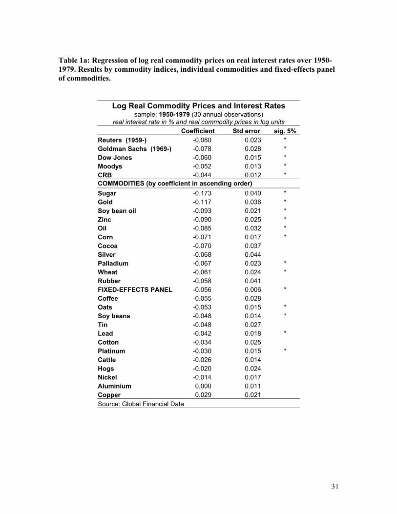
Table 1a: Regression of log real commodity prices on real interest rates over 1950-1979. Results by commodity indices, individual commodities and fixed-effects panel of commodities.

Log Real Commodity Prices and Interest Rates sample: 1950-1979 (30 annual observations)

real interest rate in % and real commodity prices in log units Coefficient Std error sig. 5% Reuters (1959-) -0.080 0.023 * Goldman Sachs (1969-) -0.078 0.028 * Dow Jones -0.060 0.015 * Moodys -0.052 0.013 * CRB -0.044 0.012 * COMMODITIES (by coefficient in ascending order) Sugar -0.173 0.040 * Gold -0.117 0.036 * Soy bean oil -0.093 0.021 * Zinc -0.090 0.025 * Oil -0.085 0.032 * Corn -0.071 0.017 * Cocoa -0.070 0.037 Silver -0.068 0.044 Palladium -0.067 0.023 * Wheat -0.061 0.024 * Rubber -0.058 0.041 FIXED-EFFECTS PANEL -0.056 0.006 * Coffee -0.055 0.028 Oats -0.053 0.015 * Soy beans -0.048 0.014 * Tin -0.048 0.027 Lead -0.042 0.018 * Cotton -0.034 0.025 Platinum -0.030 0.015 * Cattle -0.026 0.014 Hogs -0.020 0.024 Nickel -0.014 0.017 Aluminium 0.000 0.011 Copper 0.029 0.021 Source: Global Financial Data

31

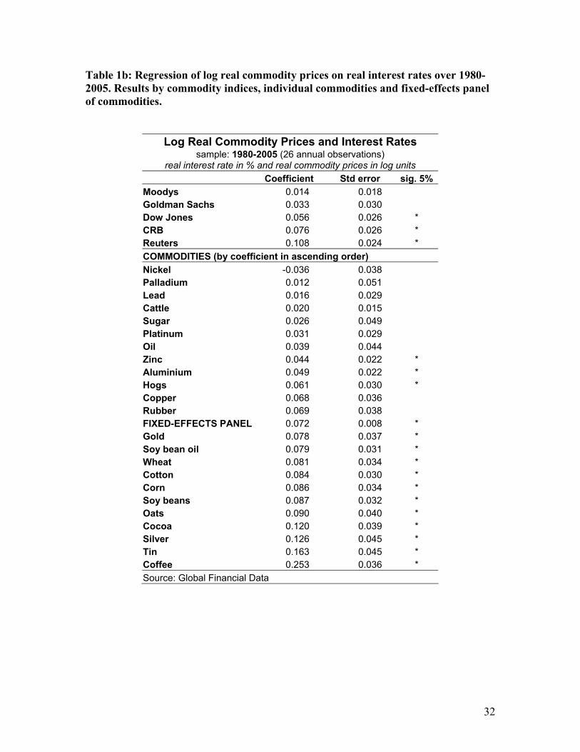
Table 1b: Regression of log real commodity prices on real interest rates over 1980-2005. Results by commodity indices, individual commodities and fixed-effects panel of commodities.

Log Real Commodity Prices and Interest Rates sample: 1980-2005 (26 annual observations)

real interest rate in % and real commodity prices in log units Coefficient Std error sig. 5% Moodys 0.014 0.018 Goldman Sachs 0.033 0.030 Dow Jones 0.056 0.026 * CRB 0.076 0.026 * Reuters 0.108 0.024 * COMMODITIES (by coefficient in ascending order) Nickel -0.036 0.038 Palladium 0.012 0.051 Lead 0.016 0.029 Cattle 0.020 0.015 Sugar 0.026 0.049 Platinum 0.031 0.029 Oil 0.039 0.044 Zinc 0.044 0.022 * Aluminium 0.049 0.022 * Hogs 0.061 0.030 * Copper 0.068 0.036 Rubber 0.069 0.038 FIXED-EFFECTS PANEL 0.072 0.008 * Gold 0.078 0.037 * Soy bean oil 0.079 0.031 * Wheat 0.081 0.034 * Cotton 0.084 0.030 * Corn 0.086 0.034 * Soy beans 0.087 0.032 * Oats 0.090 0.040 * Cocoa 0.120 0.039 * Silver 0.126 0.045 * Tin 0.163 0.045 * Coffee 0.253 0.036 * Source: Global Financial Data

32

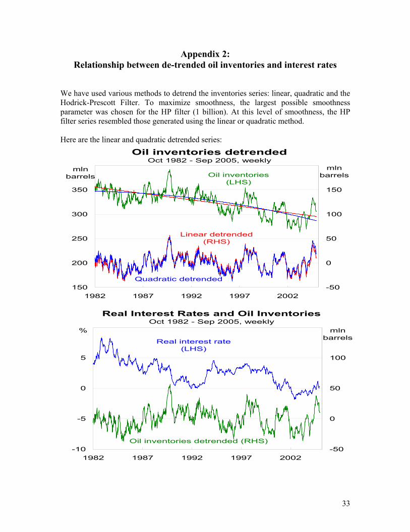
Appendix 2: Relationship between de-trended oil inventories and interest rates

We have used various methods to detrend the inventories series: linear, quadratic and the Hodrick-Prescott Filter. To maximize smoothness, the largest possible smoothness parameter was chosen for the HP filter (1 billion). At this level of smoothness, the HP filter series resembled those generated using the linear or quadratic method. Here are the linear and quadratic detrended series:

Oil inventories detrendedOct 1982 - Sep 2005, weekly

150

200

250

300

350

1982 1987 1992 1997 2002-50

0

50

100

150

Quadratic detrended

mln barrels

mln barrels

Real Interest Rates and Oil InventoriesOct 1982 - Sep 2005, weekly

-10

-5

0

5

1982 1987 1992 1997 2002-50

0

50

100

Real interest rate(LHS)

% mbarrels

Linear detrended (RHS)

Oil inventories (LHS)

Oil inventories detrended (RHS)

ln

33

Regressions Six regressions have been estimated to explore this relationship.

In regression 1, there is no detrending. In regressions 2 & 3, linear (αt) or quadratic trends (αt + βt2) are included as

extra regressors. In regressions 4 - 6, I use a two step procedure, first detrending the inventories

series and then estimating the relationship. When the linear detrending method is used, there is a significant negative relationship between the real rate and inventories. However, this result is not robust to the use of alternative detrending methods, if one fails to control for other important influences on inventory demand.

Table 4: Relationship between oil inventories and interest rates

Regressand Regressors Real rate coefficient

Standard error

Sig. at 10%

1. Inventories Real rate 5.96 0.29 *

2. Inventories Real rate & linear trend -0.69 0.35 *

3. Inventories Real rate & quadratic trend -0.36 0.35

4. Linear detrended inventories Real rate -0.31 0.23

5. Quadratic detrended inventories Real rate -0.17 0.23

6. HP detrended inventories Real rate 0.04 0.22

Appendix 3: Relationship between Inventories and Real Interest Rates

using Detrended Inventories: Controlling for Additional Regressors This appendix presents the results of a model of oil inventories, using the following regressors:

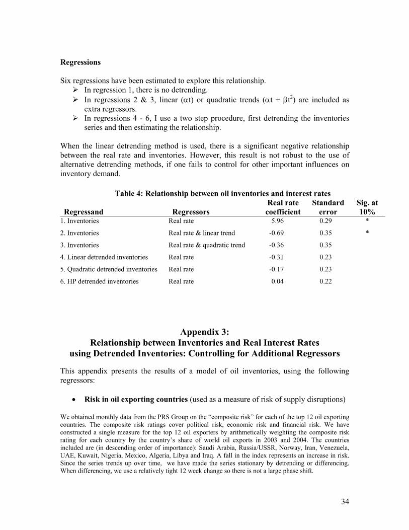
• Risk in oil exporting countries (used as a measure of risk of supply disruptions) We obtained monthly data from the PRS Group on the “composite risk” for each of the top 12 oil exporting countries. The composite risk ratings cover political risk, economic risk and financial risk. We have constructed a single measure for the top 12 oil exporters by arithmetically weighting the composite risk rating for each country by the country’s share of world oil exports in 2003 and 2004. The countries included are (in descending order of importance): Saudi Arabia, Russia/USSR, Norway, Iran, Venezuela, UAE, Kuwait, Nigeria, Mexico, Algeria, Libya and Iraq. A fall in the index represents an increase in risk. Since the series trends up over time, we have made the series stationary by detrending or differencing. When differencing, we use a relatively tight 12 week change so there is not a large phase shift.

34

Risk in top 12 Oil ExportersMonthly, weighted by 2003-04 oil exports

-4

0

4

8

12

1981 1986 1991 1996 2001-30

-20

-10

0

10Quadratic detrended (RHS)

logunits units

12 week change (LHS)

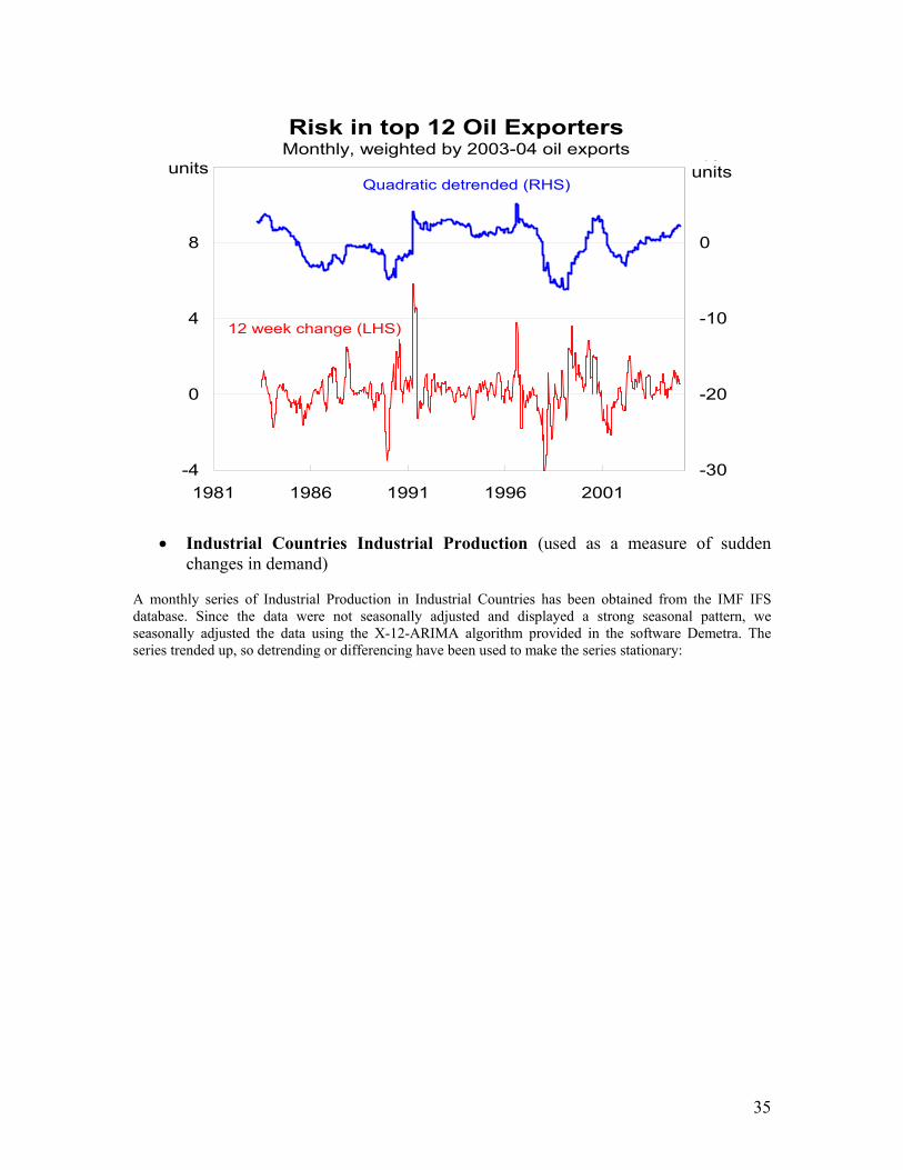
• Industrial Countries Industrial Production (used as a measure of sudden changes in demand)

A monthly series of Industrial Production in Industrial Countries has been obtained from the IMF IFS database. Since the data were not seasonally adjusted and displayed a strong seasonal pattern, we seasonally adjusted the data using the X-12-ARIMA algorithm provided in the software Demetra. The series trended up, so detrending or differencing have been used to make the series stationary:

35

Log Industrial Countries IPMonthly

-0.04

-0.02

0.00

0.02

0.04

0.06

1981 1986 1991 1996 2001-0.4

-0.3

-0.2

-0.1

0.0

0.1Quadratic detrended (RHS)

loglog

12 week change (LHS)

Quadratic detrended inventories (LHS)

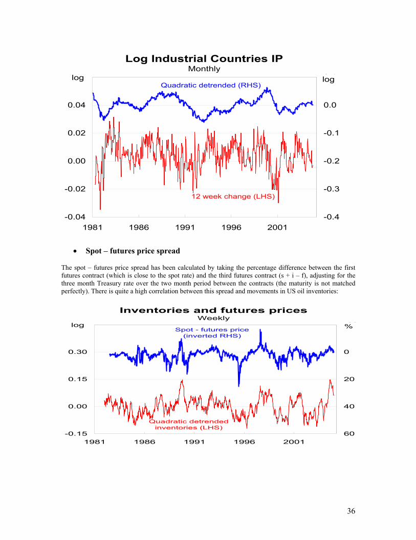
• Spot – futures price spread The spot – futures price spread has been calculated by taking the percentage difference between the first futures contract (which is close to the spot rate) and the third futures contract (s + i – f), adjusting for the three month Treasury rate over the two month period between the contracts (the maturity is not matched perfectly). There is quite a high correlation between this spread and movements in US oil inventories:

Inventories and futures pricesWeekly

-0.15

0.00

0.15

0.30

0.45

1981 1986 1991 1996 2001

-20

0

20

40

60

Spot - futures price (inverted RHS)

%log

36

Regression results

The relationship between weekly oil inventories and real interest rates is estimated controlling for the three regressors described above. When included individually, the spot-futures price spread is significant with the expected sign (when the spot price rises relative to the futures price, oil inventories fall). The 12-week change in oil exporter risk is also significant with the expected sign (a negative change in the risk rating leads to an increase in oil inventories). However, Industrial production is not significant. The real interest rate coefficient is negative in all these regressions, but is not significant.

When all the regressors are included simultaneously (either in levels OR in changes), the spot-futures spread and risk are both significant with the expected sign. The real rate coefficient is negative and significant. When lagged inventories are added, the real rate coefficient is no longer significant. When the spot-futures spread is assumed to be endogenous and IP and risk are used as instruments, the real rate coefficient is not significant.

Table 5a: Relationship between inventories and interest rates -- Weekly data (1114-1190 observations depending on data availability)

Non-stationary variables detrended by including quadratic terms in each regression

Real rate Spot-

futures IP ∆ IP Risk ∆ risk Inventories

(t-1) -0.064 Real rate only

0.097 -0.093 -0.760*

Spot-futures spread 0.077 0.039

-0.057 0.008 IP

0.101 0.059 -0.014 -0.178 12 week ∆ IP

0.103 0.136 -0.095 0.000

oil exporter risk 0.103 0.001

-0.192 -0.009* 12 week ∆ oil exporter risk 0.100 0.001

-0.394* -0.821* 0.397* -0.002* Spot-futures, IP, risk

0.089 0.041 0.062 0.001 -0.056 -0.079* 0.052* 0.000 0.931* Spot-futures, IP, risk and lagged

inventories 0.032 0.013 0.020 0.000 0.009 -0.211* -0.727* 0.131 -0.005* Spot-futures, ∆ IP, ∆ risk

0.085 0.040 0.126 0.001 -0.017 -0.071* 0.009 0.000 0.937* Spot-futures, ∆ IP, ∆ risk and

lagged inventories 0.032 0.012 0.045 0.000 0.009 Instrumental Variables

-0.068 0.343 Spot-futures; instruments: IP and risk 0.124 0.178

-0.159 -1.313* Spot-futures; instruments: ∆ IP and ∆ risk 0.102 0.212 Asterisks indicate significance at the 5% level of significance.

37

38

The results are reasonably similar when the data are detrended by including quadratic terms in each regression or through a first stage regression of each non-stationary regressor on a quadratic trend, with the residuals used in the second stage regression where inventories is the regressand.

Table 5b: Relationship between inventories and interest rates -- Weekly data Inventories, IP and oil exporter risk detrended using first stage regressions with quadratic trends

Real rate Spot-

futures IP ∆ IP Risk ∆ risk Inventories

(t-1) -0.031 Real rate only

0.065 0.021 -0.754*

Spot-futures spread 0.053 0.039 0.011 -0.003

IP 0.065 0.058 0.043 -0.200 12 week ∆ IP 0.070 0.133

-0.154* 0.000 oil exporter risk

0.076 0.001 -0.226* -0.009* 12 week ∆ oil exporter risk

0.077 0.001 -0.131* -0.806* 0.304* -0.002*

Spot-futures, IP, risk 0.067 0.042 0.062 0.001

-0.027 -0.076* 0.044* 0.000 0.933* Spot-futures, IP, risk and lagged inventories 0.023 0.013 0.019 0.000 0.009

-0.066 -0.723* 0.089 -0.005* Spot-futures, ∆ IP, ∆ risk 0.065 0.041 0.127 0.001

-0.003 -0.070* 0.006 0.000 0.937* Spot-futures, ∆ IP, ∆ risk and lagged inventories 0.024 0.012 0.044 0.000 0.009 Instrumental Variables

-0.145 0.282 Spot-futures; instruments: IP and risk 0.086 0.179

0.076 -1.368* Spot-futures; instruments: ∆ IP and ∆ risk 0.072 0.231 Asterisks indicate significance at the 5% level of significance.

Appendix 4 Relationship between Agricultural Inventories and Real

Interest Rates, using Detrended Inventories

Annual inventories data were obtained from the US Department of Agriculture for 12 agricultural commodities. For comparative purposes, we also include results using a series for petroleum inventories from the Energy Department. To make the results easier to compare across commodities, we logged the inventories series, so the coefficients are semi-elasticities. Quarterly inventories data are available for some commodities, but the seasonal patterns are extremely strong, so we converted all the commodities to a common annual frequency.

39

Five regressions have been estimated to explore this relationship for each commodity:

In regression 1, there is no detrending. In regressions 2 & 3, linear (αt) or quadratic trends (αt + βt2) are included as

extra regressors. Regressions 4 & 5 use a two step procedure, first detrending the inventories series

and then estimating the relationship. The data suggest no systematic negative relationship between real interest rates and

agricultural inventories. The different specifications do not appear to have a significant effect on the results. The relationship has also been estimated for the fixed effects panel of the nine commodities with data available from 1950-2004. This sample is broken in 1982 to test for any effect from the change in monetary policy regime. The results suggest there is a spurious positive relationship between interest rates and inventories. The results for agricultural inventories should not be taken too seriously as we were unable to control for risk or other important variables.

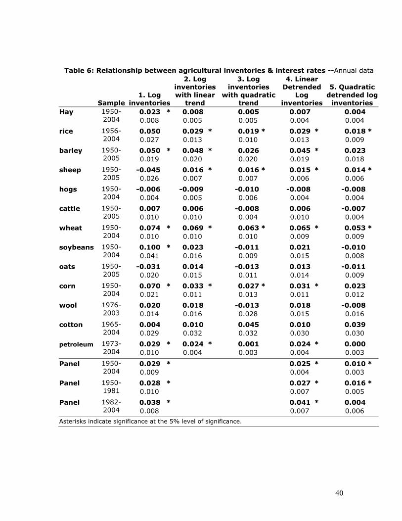
40

Table 6: Relationship between agricultural inventories & interest rates --Annual data

Sample 1. Log

inventories

2. Log inventories with linear

trend

3. Log inventories

with quadratic trend

4. Linear Detrended

Log inventories

5. Quadratic detrended log

inventories Hay 0.023 * 0.008 0.005 0.007 0.004

1950-2004 0.008 0.005 0.005 0.004 0.004

rice 0.050 0.029 * 0.019 * 0.029 * 0.018 *

1956-2004 0.027 0.013 0.010 0.013 0.009

barley 0.050 * 0.048 * 0.026 0.045 * 0.023

1950-2005 0.019 0.020 0.020 0.019 0.018

sheep -0.045 0.016 * 0.016 * 0.015 * 0.014 *

1950-2005 0.026 0.007 0.007 0.006 0.006

hogs -0.006 -0.009 -0.010 -0.008 -0.008

1950-2004 0.004 0.005 0.006 0.004 0.004

cattle 0.007 0.006 -0.008 0.006 -0.007

1950-2005 0.010 0.010 0.004 0.010 0.004

wheat 0.074 * 0.069 * 0.063 * 0.065 * 0.053 *

1950-2004 0.010 0.010 0.010 0.009 0.009

soybeans 0.100 * 0.023 -0.011 0.021 -0.010

1950-2004 0.041 0.016 0.009 0.015 0.008

oats -0.031 0.014 -0.013 0.013 -0.011

1950-2005 0.020 0.015 0.011 0.014 0.009

corn 0.070 * 0.033 * 0.027 * 0.031 * 0.023

1950-2004 0.021 0.011 0.013 0.011 0.012

wool 0.020 0.018 -0.013 0.018 -0.008

1976-2003 0.014 0.016 0.028 0.015 0.016

cotton 0.004 0.010 0.045 0.010 0.039

1965-2004 0.029 0.032 0.032 0.030 0.030

petroleum 0.029 * 0.024 * 0.001 0.024 * 0.000

1973-2004 0.010 0.004 0.003 0.004 0.003

Panel 0.029 * 0.025 * 0.010 *

1950-2004 0.009 0.004 0.003

Panel 0.028 * 0.027 * 0.016 *

1950-1981 0.010 0.007 0.005

Panel 0.038 * 0.041 * 0.004

1982-2004 0.008 0.007 0.006

Asterisks indicate significance at the 5% level of significance.