Embed Size (px)
Citation preview
350
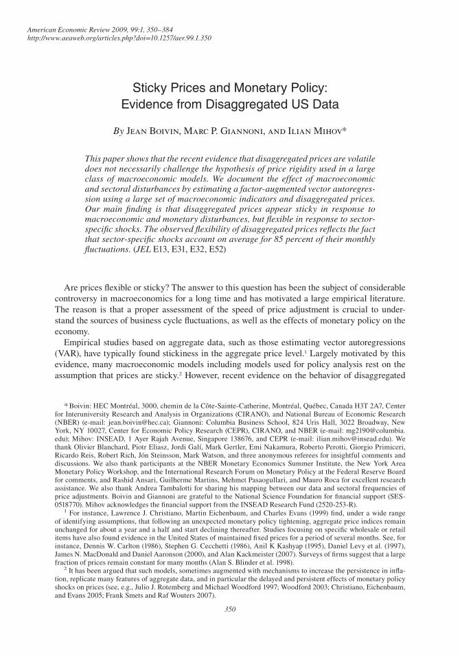
American Economic Review 2009, 99:1, 350–384http://www.aeaweb.org/articles.php?doi=10.1257/aer.99.1.350
Are prices flexible or sticky? The answer to this question has been the subject of considerable controversy in macroeconomics for a long time and has motivated a large empirical literature. The reason is that a proper assessment of the speed of price adjustment is crucial to under-stand the sources of business cycle fluctuations, as well as the effects of monetary policy on the economy.
Empirical studies based on aggregate data, such as those estimating vector autoregressions (VAR), have typically found stickiness in the aggregate price level.1 Largely motivated by this evidence, many macroeconomic models including models used for policy analysis rest on the assumption that prices are sticky.2 However, recent evidence on the behavior of disaggregated
1 For instance, Lawrence J. Christiano, Martin Eichenbaum, and Charles Evans (1999) find, under a wide range of identifying assumptions, that following an unexpected monetary policy tightening, aggregate price indices remain unchanged for about a year and a half and start declining thereafter. Studies focusing on specific wholesale or retail items have also found evidence in the United States of maintained fixed prices for a period of several months. See, for instance, Dennis W. Carlton (1986), Stephen G. Cecchetti (1986), Anil K Kashyap (1995), Daniel Levy et al. (1997), James N. MacDonald and Daniel Aaronson (2000), and Alan Kackmeister (2007). Surveys of firms suggest that a large fraction of prices remain constant for many months (Alan S. Blinder et al. 1998).
2 It has been argued that such models, sometimes augmented with mechanisms to increase the persistence in infla-tion, replicate many features of aggregate data, and in particular the delayed and persistent effects of monetary policy shocks on prices (see, e.g., Julio J. Rotemberg and Michael Woodford 1997; Woodford 2003; Christiano, Eichenbaum, and Evans 2005; Frank Smets and Raf Wouters 2007).
Sticky Prices and Monetary Policy: Evidence from Disaggregated US Data
By Jean Boivin, Marc P. Giannoni, and Ilian Mihov*
This paper shows that the recent evidence that disaggregated prices are volatile does not necessarily challenge the hypothesis of price rigidity used in a large class of macroeconomic models. We document the effect of macroeconomic and sectoral disturbances by estimating a factor-augmented vector autoregres-sion using a large set of macroeconomic indicators and disaggregated prices. Our main finding is that disaggregated prices appear sticky in response to macroeconomic and monetary disturbances, but flexible in response to sector-specific shocks. The observed flexibility of disaggregated prices reflects the fact that sector-specific shocks account on average for 85 percent of their monthly fluctuations. (JEL E13, E31, E32, E52)
* Boivin: HEC Montréal, 3000, chemin de la Côte-Sainte-Catherine, Montréal, Québec, Canada H3T 2A7, Center for Interuniversity Research and Analysis in Organizations (CIRANO), and National Bureau of Economic Research (NBER) (e-mail: [email protected]); Giannoni: Columbia Business School, 824 Uris Hall, 3022 Broadway, New York, NY 10027, Center for Economic Policy Research (CEPR), CIRANO, and NBER (e-mail: [email protected]); Mihov: INSEAD, 1 Ayer Rajah Avenue, Singapore 138676, and CEPR (e-mail: [email protected]). We thank Olivier Blanchard, Piotr Eliasz, Jordi Galí, Mark Gertler, Emi Nakamura, Roberto Perotti, Giorgio Primiceri, Ricardo Reis, Robert Rich, Jón Steinsson, Mark Watson, and three anonymous referees for insightful comments and discussions. We also thank participants at the NBER Monetary Economics Summer Institute, the New York Area Monetary Policy Workshop, and the International Research Forum on Monetary Policy at the Federal Reserve Board for comments, and Rashid Ansari, Guilherme Martins, Mehmet Pasaogullari, and Mauro Roca for excellent research assistance. We also thank Andrea Tambalotti for sharing his mapping between our data and sectoral frequencies of price adjustments. Boivin and Giannoni are grateful to the National Science Foundation for financial support (SES-0518770). Mihov acknowledges the financial support from the INSEAD Research Fund (2520-253-R).
VOL. 99 NO. 1 351BOiViN ET AL.: STicky PRicES ANd MONETARy POLicy
prices suggests that prices are much more volatile than conventionally assumed in studies based on aggregate data. For instance, Mark Bils and Peter J. Klenow (2004), looking at 350 categories of consumer goods and services that cover about 70 percent of US consumer expenditures, esti-mate that the median time between price changes is 4.3 months.3 They argue that sectoral infla-tion rates are much more volatile and short-lived than implied by sticky-price models, thereby casting doubts on the validity of such models. Klenow and Kryvtsov (2008) document that when prices change, they change by about 14 percent on average.4
The goal of this paper is to show empirically that once we distinguish between macroeco-nomic and sector-specific fluctuations, the fact that prices change frequently at the disaggregate level does not imply that prices are flexible in the face of macroeconomic shocks. In fact, we argue that the flexibility of disaggregated prices is perfectly compatible with stickiness of aggre-gate price indices.
One limitation of the existing evidence, such as that of Bils and Klenow (2004) or Klenow and Kryvtsov (2008), is that while they provide a careful description of individual prices move-ments, they do not distinguish between sector-specific and aggregate sources of fluctuations. It is thus not possible to infer from these studies whether sectoral prices respond rapidly or slowly, or strongly or moderately, to macroeconomic shocks. To reconcile the evidence on disaggregated and aggregate prices, it is crucial to properly assess the relative importance of the sector-specific and macroeconomic fluctuations in prices series.
In addition, while aggregate inflation is often argued to be persistent over long samples,5 dis-aggregated series reveal much more transient fluctuations. The apparent persistence of aggregate inflation may reflect heterogeneity across sectors or a structural break in the mean inflation dur-ing the sample.6 Yet, the differences in inflation persistence at the aggregate and disaggregate level may also be due to different responses to macroeconomic and sector-specific shocks.
In this paper, we disentangle the fluctuations in disaggregated US consumer and producer prices that are due to aggregate macroeconomic factors from those due to sectoral conditions. We do so by estimating a factor-augmented vector autoregression (FAVAR) that relates a large panel of monthly economic indicators and individual price series to a relatively small number of estimated common factors summarizing macroeconomic forces. This framework allows us to assess the relative importance of macroeconomic and sectoral factors in explaining disaggre-gated price fluctuations and inflation persistence. Using this, we can analyze the typical response of disaggregated prices to macroeconomic shocks and to sector-specific shocks.
We also estimate the effects of US monetary policy on disaggregated prices after identifying monetary policy shocks using the information from the entire dataset. We study the magnitude of
3 The median duration remains less than five months when they account for temporary sales. More recently, how-ever, Emi Nakamura and Jón Steinsson (2008), analyzing CPI microdata, argue that the median duration is between 8 and 11 months when they exclude sales and price changes due to product substitutions. Klenow and Oleksiy Kryvtsov (2008) also find longer median duration between price changes of about 7.2 months when sale prices are excluded.
The duration between price changes varies, considerably however, across sectors. According to Bils and Klenow (2004), it ranges from less than a month (for gasoline prices) to more than 80 months (coin-operated apparel laundry and dry cleaning).
4 They estimate this change to be 11.3 percent when adjusting for temporary sales. Mikhail Golosov and Robert E. Lucas Jr. (2007), in turn, calibrate a menu-cost model with both aggregate and idiosyncratic shocks to match these facts, and find that monetary policy shocks have large and rapid effects on aggregated prices but only very little effect on economic activity.
5 See, e.g., Jeffrey C. Fuhrer and George R. Moore 1995; Jordi Galí and Mark Gertler 1999; Timothy Cogley and Thomas J. Sargent 2002, 2005; Christopher A. Sims 2002; James H. Stock 2002; Andrew T. Levin and Jeremy Piger 2003; Todd E. Clark 2006; Frederic Pivetta and Ricardo Reis 2007.
6 Clive Granger (1980), Hashem M. Pesaran and Ron Smith (1995), and Jean Imbs et al. (2005) point out that the persistence of aggregate series should not be interpreted as the average persistence of individual series in the presence of heterogenous dynamics. Cogley and Sargent (2002, 2005), Levin and Piger (2003), and Clark (2006) find that infla-tion persistence drops when they allow for changes in mean inflation over time.
MARch 2009352 ThE AMERicAN EcONOMic REViEW
the price responses to monetary policy shocks, and whether monetary policy has delayed effects on prices. While extensive research has attempted to characterize the effects of monetary policy on macroeconomic indicators, little research has analyzed its effects on disaggregated prices. Two exceptions are Bils, Klenow, and Kryvtsov (2003) and Nathan S. Balke and Mark A. Wynne (2007). These authors estimate the responses of individual prices to a monetary policy shock by appending individual price series to a separately estimated VAR. However, their estimated price responses display a considerable “price puzzle,” i.e., a price increase following an unex-pected monetary policy tightening, which stands in sharp contrast to predictions of conventional models. As argued in Sims (1992) and Ben S. Bernanke, Boivin, and Piotr Eliasz (2005), such evidence of a price puzzle may be indicative of VAR misspecification due, e.g., to the lack of information considered in the VAR estimation. In the context of our data-rich FAVAR, this risk of misspecification is reduced, as we make an attempt to use all of the available information in the estimation.
Our main finding is that disaggregated prices appear sticky in response to macroeconomic fluctuations, and to monetary policy in particular, but flexible in response to sector-specific shocks. Importantly, we show that, although the implications for macroeconomic modeling are drastically different, these findings are consistent with the evidence reported in Bils and Klenow (2004). The reason is that macroeconomic fluctuations explain on average only 15 percent of the variation in monthly individual prices. So most of the fluctuations in disaggregated prices reflect sector-specific shocks to which prices are adjusting quickly, and possibly (in part) sampling error in measured disaggregated prices. Consistent with the evidence on disaggregated price series, we also find considerable disparities in the magnitude of price changes and in the persistence of inflation across price categories, both for consumer and producer prices. These disparities are due, to a large extent, to differences in the volatility of sector-specific components, and only little to different responses to macroeconomic factors.
The picture that emerges is thus one in which many prices fluctuate considerably in response to sector-specific shocks, but they respond only sluggishly to aggregate macroeconomic shocks such as monetary policy shocks. The relative importance of sector-specific shocks can explain why, at the disaggregated level, individual prices are found to adjust relatively frequently, while estimates of the degree of price rigidity are much higher when based on aggregate data. The sluggishness in price responses to macroeconomic shocks explains why models that assume considerable price stickiness have often been successful at replicating the effects of monetary policy shocks.
After documenting the responses of prices to a monetary policy shock, we attempt to provide an explanation for the cross-sectional dispersion of price responses. To this end, we collect data on industry characteristics that are related to various theories of price stickiness. We find that the observed dispersion in the reaction of producer prices is explained in large measure by the degree of market power; that prices in sectors with volatile idiosyncratic shocks react relatively more rapidly to aggregate monetary policy shocks; and that consumption categories in which prices fall the most following a monetary policy shock tend to be those in which quantities con-sumed fall the least. Finally, we find that the idiosyncratic components of prices and quantities move mostly in opposite directions, suggesting that idiosyncratic shocks may be largely supply-type shocks.
The rest of the paper is organized as follows. Section I reviews the econometric framework, by discussing the formulation and estimation of the FAVAR. In Section II, we discuss various datasets used in our estimation. Section III presents empirical results about the sources of fluc-tuations in disaggregated prices. It includes a description of the price responses to sector-spe-cific shocks and to macroeconomic fluctuations. Section IV investigates the effects of monetary policy shocks and relates the responses of producer prices in various sectors to industry
VOL. 99 NO. 1 353BOiViN ET AL.: STicky PRicES ANd MONETARy POLicy
characteristics. Section V reports some robustness results, including results for the post-1984 period. Section VI concludes by discussing various potential avenues to reconcile these results with existing theories.
I. Econometric Framework: FAVAR
The empirical framework that we consider is based on the FAVAR model described in Bernanke, Boivin, and Eliasz (2005) (BBE). One of its key features is to provide estimates of macroeconomic factors that affect the data of interest by systematically and consistently exploit-ing all information from a large set of economic indicators. In our application, we estimate the empirical model by exploiting information from a large number of macroeconomic indicators, as well as from disaggregated data. This framework is particularly well suited to decompose the fluctuations of each series into a common and a series-specific component. It also allows us to characterize the response of all data series to macroeconomic disturbances, such as monetary policy shocks. As BBE argue, this framework should lead to a better identification of the policy shock than standard VARs, because it explicitly recognizes the large information set that the Federal Reserve and financial market participants exploit in practice, and also because it does not require taking a stand on the appropriate measures of prices and real activity which can simply be treated as latent common components. A natural by-product of the estimation is to obtain impulse response functions for any variables included in the dataset. In particular, this allows us to document the effect of monetary policy on disaggregated prices.
We provide only a general description of our implementation of the empirical framework and refer the interested reader to BBE for additional details. We assume that the economy is affected by a vector Ct of common components to all variables entering the dataset. Since we will be interested in characterizing the effects of monetary policy, this vector of common components includes a measure of the stance of monetary policy. As in most related VAR applications, we assume that the federal funds rate, Rt, is the policy instrument. It will be allowed to have per-vasive effect throughout the economy and will thus be considered a common component of all variables entering the dataset. The rest of the common dynamics are captured by a k × 1 vector of unobserved factors Ft, where k is relatively small. These unobserved factors may reflect gen-eral economic conditions such as “economic activity,” the “general level of prices,” and the level of “productivity,” which are not easily captured by a few time series, but rather by a wide range of economic variables. We assume that the joint dynamics of Ft and Rt are given by
(1) Ct = Φ(L)Ct−1 + vt
where
Ft Ct = c d ,
Rt
and Φ(L) is a conformable lag polynomial of finite order which may contain a priori restrictions, as in standard structural VARs. The error term vt is i.i.d. with mean zero.
The system (1) is a VAR in Ct. The additional difficulty, with respect to standard VARs, however, is that the factors Ft are unobservable. We assume that the factors summarize the infor-mation contained in a large number of economic variables. We denote by X t this N × 1 vector of “informational” variables, where N is assumed to be “large,” i.e., N >> k + 1. We assume,
MARch 2009354 ThE AMERicAN EcONOMic REViEW
furthermore, that the large set of observable “informational” series Xt is related to the common factors according to
(2) Xt = ΛCt + et,
where Λ is an N × (k + 1) matrix of factor loadings, and the N × 1 vector et contains series-specific components that are uncorrelated with the common components Ct. These series-spe-cific components are allowed to be serially correlated and weakly correlated across indicators. Equation (2) reflects the fact that the elements of Ct, which in general are correlated, represent pervasive forces that drive the common dynamics of Xt. Conditional on the observed federal funds rate Rt, the variables in Xt are thus noisy measures of the underlying unobserved factors Ft. Note that it is in principle not restrictive to assume that Xt depends only on the current values of the factors, as Ft can always capture arbitrary lags of some fundamental factors.7
As in BBE, we estimate our empirical model using a variant of a two-step principal com-ponent approach. In the first step, we extract principal components from the large dataset Xt to obtain consistent estimates of the common factors. Stock and Watson (2002) show that the principal components consistently recover the space spanned by the factors when N is large and the number of principal components used is at least as large as the true number of factors. In the second step, we add the federal funds rate to the estimated factors, and estimate the structural VAR (1). Our implementation differs slightly from that of BBE as we impose the constraint that the federal funds rate is one of the factors in the first-step estimation.8 This guarantees that the estimated latent factors recover dimensions of the common dynamics not captured by the federal funds rate.9
This procedure has the advantages of being computationally simple and easy to implement. As discussed by Stock and Watson (2002), it also imposes few distributional assumptions and allows for some degree of cross-correlation in the idiosyncratic error term et. Boivin and Serena Ng (2005) document the good forecasting performance of this estimation approach compared to some alternatives.10
II. Data
The dataset used in the estimation of our FAVAR is a balanced panel of 653 monthly series, for the period running from 1976:1 to 2005:6. The choice of the starting date reflects our desire to maximize the sample length while considering as large a number of disaggregated price series as possible. Indeed, a significant number of the disaggregated producer price indices start in
7 This is why Stock and Mark W. Watson (1999) refer to (2) as a dynamic factor model.8 We thank Olivier Blanchard for pointing us in this direction. In contrast to the approach adopted here, BBE do not
impose the constraint that the federal funds rate is one of the common components in the first step. They instead remove the federal funds rate from the space covered by the principal components, by performing a transformation of the prin-cipal components exploiting the different behavior of what they call “slow-moving” and “fast-moving” variables, in the second step. Our approach and that of BBE provide, however, very similar results (see the working paper version of this paper, Boivin, Giannoni and Mihov (2007), for an application of the BBE estimation approach).
9 More specifically, we adopt the following procedure in the first step of the estimation. Starting from an initial estimate of Ft, denoted by Ft
(0) and obtained as the first k principal components of Xt, we iterate through the follow-ing steps: (i) we regress Xt on Ft
(0) and Rt to obtain the coefficient on Rt, which we denote by λR(0); (ii) we compute X
~t(0)
= Xt − λR(0)Rt; (iii) we estimate Ft
(1) as the first k principal components of X~
t(0); and (iv) we repeat steps (i)–(iii) multiple
times.10 Note that this two-step approach implies the presence of “generated regressors” in the second step. According to
the results of Jushan Bai (2003), the uncertainty in the factor estimates should be negligible when N is large relative to the sample length T. Still, the confidence intervals on the impulse response functions used below are based on a boot-strap procedure that accounts for the uncertainty in the factor estimation. As in BBE, the bootstrap procedure is such that (i) the factors can be resampled based on the observation equation, and (ii) conditional on the estimated factors, the VAR coefficients in the transition equation are bootstrapped as in Lutz Kilian (1998).
VOL. 99 NO. 1 355BOiViN ET AL.: STicky PRicES ANd MONETARy POLicy
1976:1. All data have been transformed to induce stationarity. The details regarding our data as well as the transformations applied to each particular series are indicated in online Appendix B (available at http://www.aeaweb.org/articles.php?doi=10.1257/aer.99.1.350).
The dataset includes 111 updated macroeconomic indicators used by BBE, which involve sev-eral measures of industrial production, various price indices, interest rates, and employment, as well as other key macroeconomic and financial variables. These indicators have been found to collectively contain useful information about the state of the economy for the appropriate identi-fication of monetary policy shocks. We expanded the dataset of BBE in two directions.
First, we appended disaggregated data published by the Bureau of Economic Analysis (BEA) on personal consumption expenditure (PCE). Specifically, we collected 335 series on PCE prices and an equal number of series on real consumption. Among these series, 35 price series and 35 real consumption series were removed because of missing observations. In order to capture data for all expenditures reported, we removed the other series in the same categories and retained the series at the immediately higher level of aggregation. However, we removed from our data-set aggregate price and real consumption series (except for overall aggregates), so as to count only once each category in the disaggregated data. We thus ended up with 190 disaggregated PCE price series and the 190 corresponding consumption series. At the level of disaggregation considered, we have, for instance, data on new domestic autos, bicycles, shoes, cereals, fresh fruit, taxicabs, and so on. In addition, we also included four price indices and four consumption aggregates (overall PCE, durable goods, nondurable goods, and services), so that we can report some results for these aggregates.11
Second, in order to obtain a more detailed picture of the characteristics of price responses, we also collected over 600 series for producer prices at the six-digit level of North American Industry Classification System (NAICS) codes (corresponding to four-digit Standard Industrial Classification (SIC) codes). Because of changes in definitions and data coverage, we managed to obtain only 154 series for the period starting in January 1976 and ending in June 2005. The number of disaggregated producer price series available diminishes markedly if we start the sample prior to 1976.
Besides the series just mentioned and used to estimate the FAVAR, we also collected data on industry characteristics, which could help us validate or reject assumptions underlying models of price determination. The C4 ratio, provided by the US Census Bureau, reports the percent-age of total sales attributable to the four largest firms in the industry. As an alternative measure of competition, we use data on gross profit rates calculated from data published in the Annual Survey of Manufactures (ASM).12
III. Fluctuations in Disaggregated Prices: Macroeconomic Factors and Sector-Specific Shocks
The estimated system (1)–(2) allows us to analyze the sources of fluctuations in sectoral infla-tion rates. Note that for all of the price series considered, (2) implies that
(3) πit = λ′iCt + eit,
11 The inclusion of these aggregates has no noticeable impact on the estimated factors, given the large number of data series used in the estimation.
12 The calculation follows procedures of National Income and Product Accounts (NIPA) for deriving gross profit rates by subtracting employees’ compensation, cost of materials, and cost of fuels from the value of total shipments and adjusting for changes in inventories of final goods. The ASM survey provides data at the four-digit SIC level (six-digit NAICS) for the years 1997, 1998, 1999, 2000, and 2001. In the cross section, we use the time-average of the profit rates over these five years.
MARch 2009356 ThE AMERicAN EcONOMic REViEW
where πit contains the monthly log change in the respective price series. This formulation allows us to disentangle the fluctuations in sectoral inflation rates due to the macroeconomic factors—represented here by the common components Ct which have a diffuse effect on all data series—from those due to sector-specific conditions represented by the term eit. It also allows us to study to what extent the persistence in sectoral inflation rates is due to macroeconomic or sectoral shocks. Note that since Ct is a vector which may contain elements with very different dynamics and the vectors of loadings λi may differ across sectors, each sector-specific inflation rate may reveal different dynamics in response to macroeconomic disturbances.13 Recall also that the sec-tor-specific terms eit are allowed to be serially correlated and weakly correlated across sectors.
We estimated the system (1)–(2) for the period 1976:1-2005:6, using the data described above, and assuming five latent factors in the vector Ft. We experimented with more factors but none of our conclusions was affected. We used 13 lags in estimating (1).
A. Sources of Fluctuations and Persistence
In this subsection we discuss some summary statistics about the volatility and the persistence of aggregated and disaggregated monthly inflation series. The next subsection proceeds with a discussion of the effects of sector-specific and macroeconomic shocks.
1. inflation Volatility.—As is indicated in the first column of Table 1, the standard deviation of monthly aggregate inflation amounts to 0.24 percent for the overall PCE series, and ranges between 0.24 percent and 0.42 percent for the inflation rates of durable goods, nondurable goods, and services. Most of the volatility in aggregate inflation is due to fluctuations in common macro-economic factors. In fact, the R2 statistic, which measures the fraction of the variance in inflation explained by the common component λ′iCt, lies above 0.5 for all of the aggregate measures.
The picture is, however, quite different for more disaggregated inflation series which are much more volatile than aggregate series with a standard deviation of 1.15 percent on average (across sectors).14 Most of this volatility is due to sector-specific disturbances. In fact, as the lower panel of Table 1 reveals, while the mean volatility of the common component of inflation lies at 0.33 percent, the volatility of the sector-specific component is more than three times as large. In addi-tion, the R2 statistic amounts to 0.15 on average for these series, suggesting that 85 percent of the monthly disaggregated inflation fluctuations are attributable to sector-specific disturbances. The results are roughly similar for PCE and producer price index (PPI) inflation rates.
Table 1 also reveals considerable heterogeneity across sectors in inflation volatility. This is mainly due to differences in the volatility of sector-specific conditions, and much less so to dif-ferences in the response to macroeconomic fluctuations. As the sector-specific components tend to cancel each other out, inflation in the aggregate price indices ends up being less volatile than most sector-specific inflation rates.
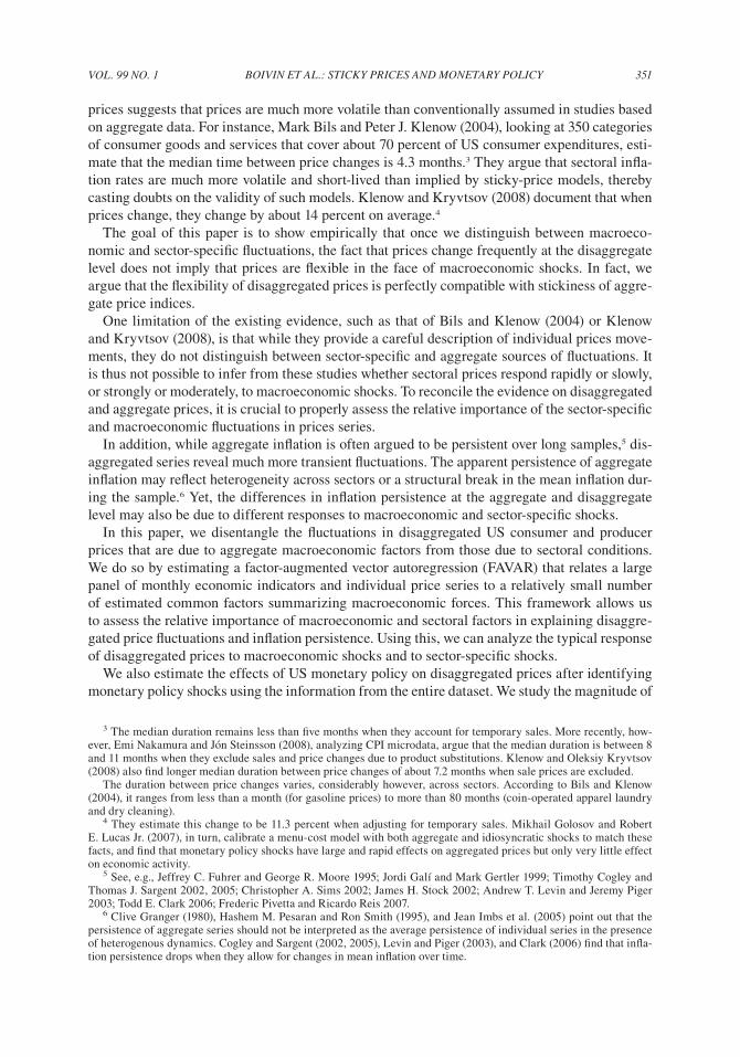
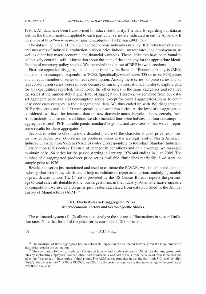
Interestingly, the volatility of the common and the sector-specific components of inflation are strongly positively correlated across sectors, as indicated in Figure 1. The correlation between the volatility of idiosyncratic shocks (Sd (ei)) and the volatility of the common component
13 In a recent paper, Reis and Watson (2007) estimate an equation of the form (3) using only disaggregate consumer price data, and decompose the term due to macroeconomic conditions, λ′iCt , into a component that involves a common change in all price categories and a component that involves relative price changes.
14 The average volatility of disaggregated PCE inflation series, weighted with expenditure shares, is somewhat lower than the unweighted average, but the overall picture remains the same for the volatility as well as for other statistics described below.
VOL. 99 NO. 1 357BOiViN ET AL.: STicky PRicES ANd MONETARy POLicy
(Sd (λ′iCt )) is high both for PCE deflators (0.74) and for PPI data (0.81) (see Table 2).15 Note that the inflation variance explained by the macroeconomic factors depends on the loadings repre-sented by the matrix Λ. One interpretation is that these loadings reflect the price-setting behavior of firms in various industries. Under this interpretation, Figure 1 reveals that firms in industries with volatile idiosyncratic shocks also respond strongly to macroeconomic shocks. This may be the case if frequent price adjustments necessitated by idiosyncratic volatility are also used as an opportunity to adjust to changes in the macroeconomic environment. That would be consistent, for instance, with a sticky price model à la Guillermo Calvo with heterogeneity in the frequency of price adjustment across sectors, as in Carlos Carvalho (2006).
The sector-specific fluctuations eit should, however, be interpreted with care as they may reflect not only structural disturbances but also measurement error in sectoral price indices. As Owen J. Shoemaker (2006) and Christian Broda and David E. Weinstein (2007) point out, the components of the consumer price index (which underlie most disaggregated PCE indices) may involve a relatively large amount of sampling error due to the fact that each month the Bureau of Labor Statistics (BLS) collects prices from a subsample of all retail prices, and not from all retail
15 From a statistical point of view, there is no reason a priori to expect that the portion of inflation volatility explained by the regression (common component) and the portion of inflation volatility explained by the error terms should be correlated across industries (or samples). Therefore, Figure 1 presents an interesting result that requires structural interpretation.
Table 1—Volatility and Persistence of Monthly Inflation Series
Standard deviation (in percent) Persistence
Common Sector- Common Sector-Inflation components specific R2 Inflation components specific
Aggregated series PCE Total 0.24 0.21 0.11 0.80 0.93 0.96 0.23 Durables 0.33 0.25 0.21 0.58 0.92 0.98 0.52 Nondurables 0.42 0.31 0.29 0.53 0.76 0.92 0.28 Services 0.24 0.19 0.14 0.64 0.94 0.98 −0.65
disaggregated series All Average 1.15 0.33 1.09 0.15 0.49 0.92 −0.07 Median 0.75 0.27 0.71 0.12 0.59 0.94 −0.01 Minimum 0.23 0.06 0.13 0.01 −3.57 0.22 −2.21 Maximum 11.68 1.86 11.61 0.73 0.96 0.99 0.85 Standard deviation 1.14 0.23 1.13 0.12 0.42 0.08 0.49
PCE Average 0.98 0.30 0.92 0.17 0.50 0.93 −0.10 Average (weighted) 0.88 0.31 0.80 0.27 0.60 0.94 0.08 Median 0.65 0.24 0.61 0.12 0.60 0.95 −0.01 Minimum 0.23 0.08 0.13 0.01 −3.57 0.22 −2.21 Maximum 11.68 1.86 11.61 0.73 0.96 0.99 0.85 Standard deviation 1.10 0.23 1.09 0.15 0.50 0.08 0.55
PPI Average 1.36 0.38 1.30 0.12 0.48 0.91 −0.04 Median 0.92 0.31 0.88 0.11 0.56 0.93 0.00 Minimum 0.35 0.06 0.30 0.01 −0.58 0.29 −1.36 Maximum 7.75 1.13 7.69 0.42 0.91 0.98 0.78 Standard deviation 1.16 0.21 1.15 0.08 0.29 0.07 0.40
Notes: Sample is 1976:1–2005:6. Inflation is measured as πit = pit − pit−1, where pit is the log of the price series i. Common components are λ′iCt. Sector-specific components are eit. R
2 statistics measure the fraction of the variance of πit explained by λ′iCt. Persistence is based on estimated AR processes with 13 lags. Weighted average of statistics for disaggregated PCE series is obtained using expenditure shares in year 2005 as weights.
MARch 2009358 ThE AMERicAN EcONOMic REViEW
prices. It is important to note, though, that the empirical framework adopted here is particularly well suited to characterize the effects of aggregate disturbances on disaggregated price series in the presence of measurement error, to the extent that such errors are series-specific. In this case, measurement error does generally not distort the estimates of the common components and the estimated effects of aggregate disturbances, even in the extreme situation in which the sector-specific components of inflation are entirely driven by measurement error.
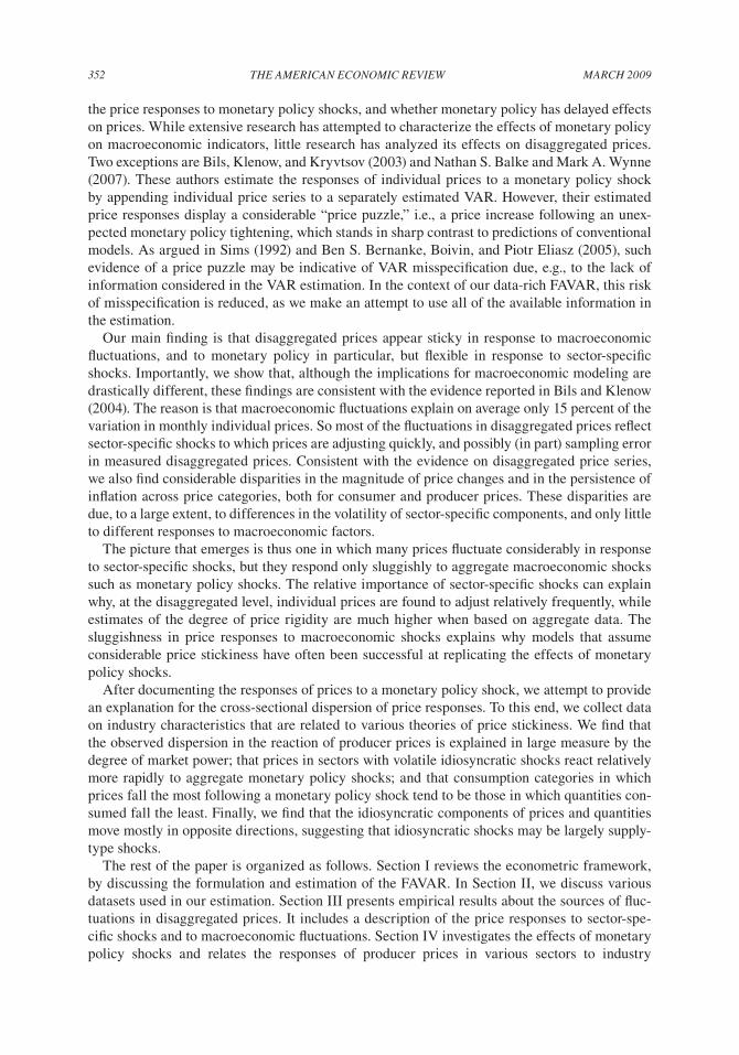
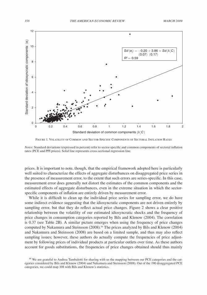
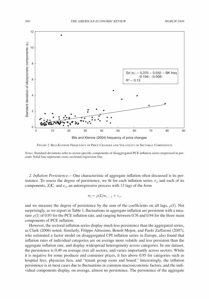
While it is difficult to clean up the individual price series for sampling error, we do have some indirect evidence suggesting that the idiosyncratic components are not driven entirely by sampling error, but that they do reflect actual price changes. Figure 2 shows a clear positive relationhip between the volatility of our estimated idiosyncratic shocks and the frequency of price changes in consumption categories reported by Bils and Klenow (2004). The correlation is 0.37 (see Table 2B). A similar picture emerges when using the frequency of price changes computed by Nakamura and Steinsson (2008).16 The prices analyzed by Bils and Klenow (2004) and Nakamura and Steinsson (2008) are based on a limited sample, and thus may also reflect sampling issues; however, these authors do actually compute the frequencies of price adjust-ment by following prices of individual products at particular outlets over time. As these authors account for goods substitutions, the frequencies of price changes obtained should thus mainly
16 We are grateful to Andrea Tambalotti for sharing with us the mapping between our PCE categories and the cat-egories considered by Bils and Klenow (2004) and Nakamura and Steinsson (2008). Out of the 190 disaggregated PCE categories, we could map 108 with Bils and Klenow’s statistics.
0
2
4
6
8
10
12
0 0.2 0.4 0.6 0.8 1 1.2 1.4 1.6 1.8 2
Standard deviation of common components (λ′i C)
Sta
ndar
d de
viat
ion
of id
iosy
ncra
tic c
ompo
nent
s (e
i)
Sd (ei) = −0.20 + 3.86 × Sd(λ′i C) (0.07) (0.17)R2 = 0.59
Figure 1. Volatility of Common and Sector-Specific Components of Sectoral Inflation Rates
Notes: Standard deviations (expressed in percent) refer to sector-specific and common components of sectoral inflation rates (PCE and PPI prices). Solid line represents cross-sectional regression line.
VOL. 99 NO. 1 359BOiViN ET AL.: STicky PRicES ANd MONETARy POLicy
reflect actual price changes, and not changes in the basket of goods considered. The positive cor-relation between the volatility of our sector-specific components and their statistics indicates that we do capture some of the actual price changes in these categories, rather than only substitution. In addition, if the sector-specific components of inflation were mostly reflecting sampling error, it would be difficult to see why their volatility is so strongly correlated with the volatility of the common component of inflation across sectors, as shown in Figure 1.
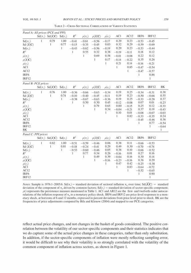
Table 2—Cross-Sectional Correlations of Various Statistics
Panel A: All prices (PcE and PPi)Sd(πi) Sd(λ′iC) Sd(ei) R2 ρ(πi) ρ(λ′iC) ρ(ei) AC1 AC12 IRF6 IRF12
Sd(πi) 1 0.79 1.00 −0.41 −0.61 −0.56 −0.17 0.29 0.23 −0.53 −0.45Sd (λ′iC) 1 0.77 −0.15 −0.35 −0.45 0.03 0.32 0.29 −0.59 −0.69Sd(ei) 1 −0.43 −0.62 −0.56 −0.19 0.29 0.23 −0.53 −0.44R2 1 0.55 0.32 0.38 −0.19 −0.11 0.18 0.12ρ(πi) 1 0.69 0.58 −0.01 −0.08 0.22 0.12ρ(λ′iC) 1 0.17 −0.14 −0.22 0.35 0.26ρ(ei) 1 0.21 0.14 −0.16 −0.21AC1 1 0.85 −0.47 −0.54AC12 1 −0.47 −0.57IRF6 1 0.86IRF12 1
Panel B: PcE pricesSd(πi) Sd(λ′iC) Sd(ei) R2 ρ(πi) ρ(λ′iC) ρ(ei) AC1 AC12 IRF6 IRF12 BK
Sd(πi) 1 0.76 1.00 −0.36 −0.66 −0.63 −0.34 0.19 0.25 −0.34 −0.31 0.38Sd (λ′iC) 1 0.74 −0.10 −0.40 −0.45 −0.11 0.19 0.23 −0.50 −0.66 0.55Sd(ei) 1 −0.38 −0.67 −0.63 −0.36 0.19 0.25 −0.33 −0.28 0.37R2 1 0.50 0.30 0.45 −0.12 −0.08 0.07 0.01 −0.23ρ(πi) 1 0.79 0.65 0.00 −0.15 0.25 0.12 −0.33ρ(λ′iC) 1 0.34 −0.04 −0.21 0.37 0.19 −0.43ρ(ei) 1 0.10 0.01 −0.08 −0.07 −0.03AC1 1 0.82 −0.33 −0.35 0.24AC12 1 −0.45 −0.46 0.36IRF6 1 0.77 −0.54IRF12 1 −0.64BK 1
Panel c: PPi pricesSd(πi) Sd(λ′iC) Sd(ei) R2 ρ(πi) ρ(λ′iC) ρ(ei) AC1 AC12 IRF6 IRF12
Sd(πi) 1 0.82 1.00 −0.51 −0.59 −0.46 0.06 0.38 0.11 −0.66 −0.53Sd (λ′iC) 1 0.81 −0.18 −0.24 −0.41 0.29 0.49 0.30 −0.70 −0.74Sd(ei) 1 −0.53 −0.60 −0.46 0.05 0.38 0.10 −0.66 −0.52R2 1 0.77 0.34 0.26 −0.16 0.01 0.27 0.16ρ(πi) 1 0.49 0.39 −0.04 0.16 0.30 0.14ρ(λ′iC) 1 −0.16 −0.23 −0.16 0.36 0.29ρ(ei) 1 0.47 0.42 −0.25 −0.38AC1 1 0.83 −0.64 −0.72AC12 1 −0.52 −0.65IRF6 1 0.90IRF12 1
Notes: Sample is 1976:1–2005:6. Sd(πi ) = standard deviation of sectoral inflation πit over time; Sd(λ′iC) = standard deviation of the component of πit driven by common factors; Sd(ei) = standard deviation of sector-specific component; ρ() represents the persistence measure mentioned in Table 1. AC1 and AR12 are the first- and twelveth-order autocor-relations of the inflation response of πit to a monetary policy shock. IRF6 and IRF12 are price-level responses to a mon-etary shock, at horizons of 6 and 12 months, expressed in percent deviations from price level prior to shock. BK are the frequencies of price adjustments computed by Bils and Klenow (2004) and mapped to our PCE categories.
MARch 2009360 ThE AMERicAN EcONOMic REViEW
2. inflation Persistence.—One characteristic of aggregate inflation often discussed is its per-sistence. To assess the degree of persistence, we fit for each inflation series πit and each of its components, λ′iCt and eit, an autoregressive process with 13 lags of the form
wt = ρ(L)wt − 1 + εt,
and we measure the degree of persistence by the sum of the coefficients on all lags, ρ(1). Not surprisingly, as we report in Table 1, fluctuations in aggregate inflation are persistent with a mea-sure ρ(1) of 0.93 for the PCE inflation rate, and ranging between 0.76 and 0.94 for the three main components of PCE inflation.
However, the sectoral inflation series display much less persistence than the aggregated series, as Clark (2006) noted. Similarly, Filippo Altissimo, Benoît Mojon, and Paolo Zaffaroni (2007), who estimated a factor model on disaggregated CPI inflation series in Europe, also found that inflation rates of individual categories are on average more volatile and less persistent than the aggregate inflation rate, and display widespread heterogeneity across categories. In our dataset, the persistence is 0.49 on average over all sectors, and varies importantly across sectors. While it is negative for some producer and consumer prices, it lies above 0.95 for categories such as hospital fees, physician fees, and “tenant group room and board.” Interestingly, the inflation persistence is in most cases due to fluctuations in common macroeconomic factors, and the indi-vidual components display, on average, almost no persistence. The persistence of the aggregate
0
2
4
6
8
10
12
0 10 20 30 40 50 60 70 80 90
Bils and Klenow (2004) frequency of price changes
Sta
ndar
d de
viat
ion
of id
iosy
ncra
tic c
ompo
nent
s (e
i)
Sd (ei) = 0.370 + 0.032 × BK freq (0.194) (0.008)R2 = 0.13
Figure 2. Bils-Klenow Frequency of Price Changes and Volatility of Sectoral Components
Notes: Standard deviations refer to sector-specific components of disaggregated PCE inflation series (expressed in per-cent). Solid line represents cross-sectional regression line.
VOL. 99 NO. 1 361BOiViN ET AL.: STicky PRicES ANd MONETARy POLicy
inflation rates thus inherits the persistence of the common component in disaggregated inflation, as the idiosyncratic components tend to average out across sectors.
3. Persistence and Volatility.—Bils and Klenow (2004) emphasize that, for a particular process for marginal costs, the Calvo model predicts that a higher degree of price stickiness reduces the impact of exogenous shocks on current inflation, but that it increases the inflation persistence.17 Thus, everything else equal, in sectors with high price stickiness, the inflation rate should display a relatively low volatility and a relatively high persistence. Bils and Klenow (2004) argue that models such as the Calvo model are rejected by the data, as they predict a strong negative cor-relation across sectors between the frequency of price adjustment and the persistence in sectoral inflation, while this correlation is positive in their data covering 123 consumer goods over the period 1995–2000, and only mildly negative in their longer dataset.
Looking at all PCE and PPI prices, we find, in line with the results of Bils and Klenow (2004), a relatively weak negative correlation (−0.19) between volatility and persistence in the sector-specific component of inflation, as Table 2A indicates. However, once we look at the common component of inflation, the persistence and the volatility of inflation are much more negatively correlated (−0.45). Focusing on the PCE prices, which we can map with the Bils and Klenow (2004) statistics, we also note from Table 2B that the persistence in the sector-specific component of inflation and the frequency of price adjustments are almost uncorrelated across categories, in contrast to the implications of the Calvo model. However, this correlation is −0.43 for the compo-nent of inflation driven by common macroeconomic shocks. This explains in part why the Calvo model is more successful in describing the volatility and persistence of inflation fluctuations generated by macroeconomic disturbances, than those generated by sector-specific shocks.
B. Effects of Macroeconomic Shocks and Sector-Specific Shocks
Prices may change for all sorts of reasons, including changes in costs, productivity, or demand for goods. While Bils and Klenow (2004) and Klenow and Kryvtsov (2008) provide very valu-able evidence that most prices are changed relatively frequently, and on average by large amounts, they do not identify the source of these changes. It is therefore not clear from these studies whether prices that tend to change frequently and by large amounts—e.g., due to large and fre-quent changes in sector-specific conditions—also change readily as a result of macroeconomic shocks. Clarifying this issue is particularly relevant to understanding the effects of monetary policy. In fact, if prices were adjusting rapidly to monetary shocks, monetary policy would have minor and only short-lived effects on economic activity, as in the model of Golosov and Lucas (2007). Our paper thus complements Bils and Klenow’s (2004) study by documenting how prices respond to sector-specific shocks and macroeconomic disturbances.
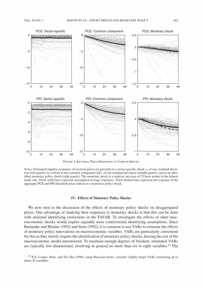
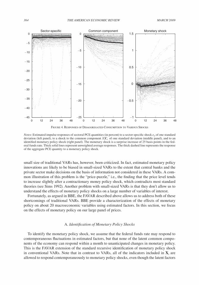
The left panels of Figure 3 report the response of each of the sectoral (log) price levels to an adverse shock to its own sector-specific component. It is the response to a drop in eit by one standard deviation. The solid lines represent the (unweighted) average responses. These prices typically respond sharply and very promptly to sector-specific disturbances, and tend to reach their new equilibrium level shortly after the shock. inflation rates show thus no persistence in response to the sector-specific shock. For PCE categories, we report in Figure 4 the responses of the corresponding quantities to an adverse sector-specific shock in consumption. Similar to
17 As they mention, under the simplifying assumption that nominal marginal costs follow a random walk for each good, the Calvo model implies an inflation process for the good i of the form πit= (1 − δi )πit−1 + δiεit, where πit is the change in the log price of good i, δi is the frequency of price adjustment or the probability that the price of good i changes in any given period, and εit is the i.i.d. growth rate of the good i’s marginal cost.
MARch 2009362 ThE AMERicAN EcONOMic REViEW
prices, quantities fall once and for all in response to such a shock. They don’t seem to revert to the initial value.
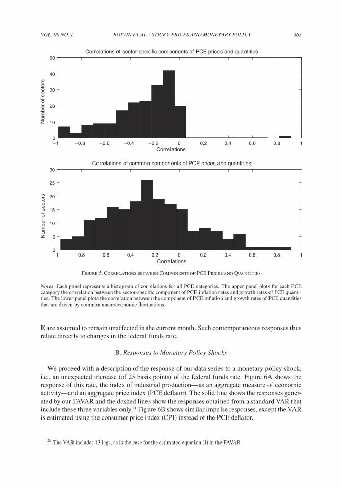
To understand better the shocks that underlie sector-specific disturbances, in Figure 5 we plot the correlation between the sector-specific component of PCE inflation rates and the cor-responding sector-specific component of PCE quantities (in growth rates). The figure reports the histogram of the correlations over all sectors, and as it demonstrates clearly, all correlations except one are negative.18 One possible explanation is that sector-specific shocks are overwhelm-ingly supply-type disturbances. This finding is consistent with Francesco Franco and Thomas Philippon (2007), who, by looking at a large panel of firms, find that permanent shocks to pro-ductivity, largely uncorrelated across firms, explain a large fraction of the firms’ dynamics. Another possibility is that disaggregated prices contain significant sampling errors, which, for given estimates of nominal expenditures, lead mechanically to inversely related estimates of real PCE. As argued earlier, however, while sampling errors are likely to affect the disaggregated PCE price indices, they are not likely to explain most of the fluctuations, given the magnitude of the sector-specific price fluctuations.
While sector-specific shocks tend to shift prices and quantities permanently to a new level, the responses to macroeconomic disturbances are very different. The middle panels of Figure 3 show the responses of each sectoral price to an innovation (of minus one standard deviation) to its common component λ′iCt .19 We do the same for the PCE quantities in Figure 4. Prices and quan-tities fall by a relatively moderate amount in the first few months after the shock, but then con-tinue to fall over the subsequent months. This reveals important sluggishness in the responses of prices to macroeconomic disturbances, and persistence in inflation rates. This contrasts sharply with the responses to sector-specific shocks.
Of course, since we don’t identify any structural macroeconomic shock in this exercise, we are describing the response to a combination of macroeconomic shocks. These figures do not allow us to exclude the possibility that there exist macroeconomic disturbances that cause a rapid and permanent change in prices. To address this shortcoming, in the next section we identify a particular macroeconomic shock, i.e., a monetary policy shock. To get a sense of the kind of macroeconomic shocks we are considering here, we note that they do have a permanent effect on both prices and quantities, and that for PCE categories, the correlation between the common component of prices and of the corresponding quantities is widely distributed over the −1 to + 1 interval (Figure 5). This suggests that the disturbances that are common to our large dataset involve both supply- and demand-type shocks.
Overall, the results of this section suggest that changes in sector-specific conditions are the most important determinants of sectoral inflation rates. Fluctuations in the common components, however, are responsible for a significant fraction of the volatility of sectoral inflation rates, and generate most of the fluctuations in aggregate inflation. In addition, sectoral prices respond very differently to sector-specific shocks and to macroeconomic shocks. While sector-specific shocks may cause large fluctuations in sectoral inflation, these fluctuations are typically short lived so that prices tend to move immediately to their new permanent level. Aggregate macroeconomic shocks instead tend to have more persistent and sluggish effects on a wide range of sectoral infla-tion rates.
18 The positive correlation refers to the category “insurance premiums for user-operated transportation.”19 The responses are computed for an innovation to the AR processes estimated on each of the components, and
discussed in Section IIIA.2.
VOL. 99 NO. 1 363BOiViN ET AL.: STicky PRicES ANd MONETARy POLicy
IV. Effects of Monetary Policy Shocks
We now turn to the discussion of the effects of monetary policy shocks on disaggregated prices. One advantage of studying their responses to monetary shocks is that this can be done with minimal identifying restrictions in the FAVAR. To investigate the effects of other mac-roeconomic shocks would require arguably more controversial identifying assumptions. Since Bernanke and Blinder (1992) and Sims (1992), it is common to use VARs to estimate the effects of monetary policy innovations on macroeconomic variables. VARs are particularly convenient for this as they merely require the identification of monetary policy shocks, leaving the rest of the macroeconomic model unrestricted. To maintain enough degrees of freedom, estimated VARs are typically low-dimensional, involving in general no more than six to eight variables.20 The
20 Eric Leeper, Sims, and Tao Zha (1996), using Bayesian priors, consider slightly larger VARs containing up to about 20 variables.
Figure 3. Sectoral Price Responses to Various Shocks
Notes: Estimated impulse responses of sectoral prices (in percent) to a sector-specific shock eit of one standard devia-tion (left panels), to a shock to the common component λ′iCt of one standard deviation (middle panels), and to an iden-tified monetary policy shock (right panels). The monetary shock is a surprise increase of 25 basis points in the federal funds rate. Thick solid lines represent unweighted average responses. Thick dashed lines represent the response of the aggregate PCE and PPI (finished) price indices to a monetary policy shock.
0 12 24 36 48−15
−10
−5
0PCE: Sector-specific
0 12 24 36 48−10
−8
−6
−4
−2
0PPI: Sector-specific
0 12 24 36 48−15
−10
−5
0PCE: Common component
0 12 24 36 48−15
−10
−5
0PPI: Common component
0 12 24 36 48−1.5
−1
−0.5
0
0.5PCE: Monetary shock
0 12 24 36 48−1
−0.5
0
0.5PPI: Monetary shock
MARch 2009364 ThE AMERicAN EcONOMic REViEW
small size of traditional VARs has, however, been criticized. In fact, estimated monetary policy innovations are likely to be biased in small-sized VARs to the extent that central banks and the private sector make decisions on the basis of information not considered in these VARs. A com-mon illustration of this problem is the “price-puzzle,” i.e., the finding that the price level tends to increase slightly after a contractionary money policy shock, which contradicts most standard theories (see Sims 1992). Another problem with small-sized VARs is that they don’t allow us to understand the effects of monetary policy shocks on a large number of variables of interest.
Fortunately, as argued in BBE, the FAVAR described above allows us to address both of these shortcomings of traditional VARs. BBE provide a characterization of the effects of monetary policy on about 20 macroeconomic variables using estimated factors. In this section, we focus on the effects of monetary policy on our large panel of prices.
A. identification of Monetary Policy Shocks
To identify the monetary policy shock, we assume that the federal funds rate may respond to contemporaneous fluctuations in estimated factors, but that none of the latent common compo-nents of the economy can respond within a month to unanticipated changes in monetary policy. This is the FAVAR extension of the standard recursive identification of monetary policy shock in conventional VARs. Note that in contrast to VARs, all of the indicators included in Xt are allowed to respond contemporaneously to monetary policy shocks, even though the latent factors
Figure 4. Responses of Disaggregated Consumption to Various Shocks
Notes: Estimated impulse responses of sectoral PCE quantities (in percent) to a sector-specific shock eit of one standard deviation (left panel), to a shock to the common component λ′iCt of one standard deviation (middle panel), and to an identified monetary policy shock (right panel). The monetary shock is a surprise increase of 25 basis points in the fed-eral funds rate. Thick solid lines represent unweighted average responses. The thick dashed line represents the response of the aggregate PCE quantity to a monetary policy shock.
0 12 24 36 48−45
−40
−35
−30
−25
−20
−15
−10
−5
0Sector-specific
0 12 24 36 48−25
−20
−15
−10
−5
0Common component
0 12 24 36 48−1
−0.5
0
0.5
1
1.5Monetary shock
VOL. 99 NO. 1 365BOiViN ET AL.: STicky PRicES ANd MONETARy POLicy
Ft are assumed to remain unaffected in the current month. Such contemporaneous responses thus relate directly to changes in the federal funds rate.
B. Responses to Monetary Policy Shocks
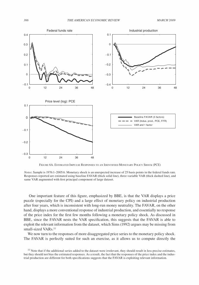
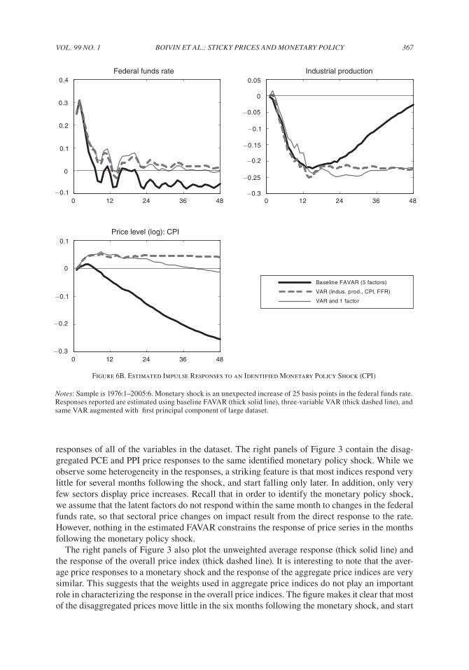
We proceed with a description of the response of our data series to a monetary policy shock, i.e., an unexpected increase (of 25 basis points) of the federal funds rate. Figure 6A shows the response of this rate, the index of industrial production—as an aggregate measure of economic activity—and an aggregate price index (PCE deflator). The solid line shows the responses gener-ated by our FAVAR and the dashed lines show the responses obtained from a standard VAR that include these three variables only.21 Figure 6B shows similar impulse responses, except the VAR is estimated using the consumer price index (CPI) instead of the PCE deflator.
21 The VAR includes 13 lags, as is the case for the estimated equation (1) in the FAVAR.
−1 −0.8 −0.6 −0.4 −0.2 0 0.2 0.4 0.6 0.8 10
10
20
30
40
50Correlations of sector-specific components of PCE prices and quantities
Correlations
−1 −0.8 −0.6 −0.4 −0.2 0 0.2 0.4 0.6 0.8 10
5
10
15
20
25
30Correlations of common components of PCE prices and quantities
Correlations
Num
ber
of s
ecto
rsN
umbe
r of
sec
tors
Figure 5. Correlations between Components of PCE Prices and Quantities
Notes: Each panel represents a histogram of correlations for all PCE categories. The upper panel plots for each PCE category the correlation between the sector-specific component of PCE inflation rates and growth rates of PCE quanti-ties. The lower panel plots the correlation between the component of PCE inflation and growth rates of PCE quantities that are driven by common macroeconomic fluctuations.
MARch 2009366 ThE AMERicAN EcONOMic REViEW
One important feature of this figure, emphasized by BBE, is that the VAR displays a price puzzle (especially for the CPI) and a large effect of monetary policy on industrial production after four years, which is inconsistent with long-run money neutrality. The FAVAR, on the other hand, displays a more conventional response of industrial production, and essentially no response of the price index for the first few months following a monetary policy shock. As discussed in BBE, since the FAVAR nests the VAR specification, this suggests that the FAVAR is able to exploit the relevant information from the dataset, which Sims (1992) argues may be missing from small-sized VARs.22
We now turn to the responses of more disaggregated price series to the monetary policy shock. The FAVAR is perfectly suited for such an exercise, as it allows us to compute directly the
22 Note that if the additional series added to the dataset were irrelevant, they should result in less precise estimates, but they should not bias the estimated responses. As a result, the fact that the responses of the price index and the indus-trial production are different for both specifications suggests that the FAVAR is exploiting relevant information.
Figure 6A. Estimated Impulse Responses to an Identified Monetary Policy Shock (PCE)
Notes: Sample is 1976:1–2005:6. Monetary shock is an unexpected increase of 25 basis points in the federal funds rate. Responses reported are estimated using baseline FAVAR (thick solid line), three-variable VAR (thick dashed line), and same VAR augmented with first principal component of large dataset.
Baseline FAVAR (5 factors)
VAR (Indus. prod., PCE, FFR)
VAR and 1 factor
0 12 24 36 48−0.1
0
0.1
0.2
0.3
0.4
Federal funds rate
0 12 24 36 48−0.4
−0.3
−0.2
−0.1
0
0.1Industrial production
0 12 24 36 48−0.3
−0.2
−0.1
0
0.1Price level (log): PCE
VOL. 99 NO. 1 367BOiViN ET AL.: STicky PRicES ANd MONETARy POLicy
responses of all of the variables in the dataset. The right panels of Figure 3 contain the disag-gregated PCE and PPI price responses to the same identified monetary policy shock. While we observe some heterogeneity in the responses, a striking feature is that most indices respond very little for several months following the shock, and start falling only later. In addition, only very few sectors display price increases. Recall that in order to identify the monetary policy shock, we assume that the latent factors do not respond within the same month to changes in the federal funds rate, so that sectoral price changes on impact result from the direct response to the rate. However, nothing in the estimated FAVAR constrains the response of price series in the months following the monetary policy shock.
The right panels of Figure 3 also plot the unweighted average response (thick solid line) and the response of the overall price index (thick dashed line). It is interesting to note that the aver-age price responses to a monetary shock and the response of the aggregate price indices are very similar. This suggests that the weights used in aggregate price indices do not play an important role in characterizing the response in the overall price indices. The figure makes it clear that most of the disaggregated prices move little in the six months following the monetary shock, and start
Figure 6B. Estimated Impulse Responses to an Identified Monetary Policy Shock (CPI)
Notes: Sample is 1976:1–2005:6. Monetary shock is an unexpected increase of 25 basis points in the federal funds rate. Responses reported are estimated using baseline FAVAR (thick solid line), three-variable VAR (thick dashed line), and same VAR augmented with first principal component of large dataset.
0 12 24 36 48−0.1
0
0.1
0.2
0.3
0.4Federal funds rate
0 12 24 36 48−0.3
−0.25
−0.2
−0.15
−0.1
−0.05
0
0.05Industrial production
0 12 24 36 48−0.3
−0.2
−0.1
0
0.1Price level (log): CPI
Baseline FAVAR (5 factors)
VAR (Indus. prod., CPI, FFR)
VAR and 1 factor
MARch 2009368 ThE AMERicAN EcONOMic REViEW
decreasing thereafter. As reported in Table 3, prices fall on average (across sectors) by only 0.03 percent after 6 months, and by 0.07 percent after the first 12 months. The drop in prices is more pronounced for producer prices than for consumer prices.
In addition, when prices start to fall following a monetary shock, they tend to decline fairly steadily for a couple of years. As reported in Table 3, the autocorrelation coefficients of inflation conditional on a monetary shock are all very high. These responses result in relatively persis-tent sectoral inflation movements, which contrast sharply with the responses to sector-specific shocks.
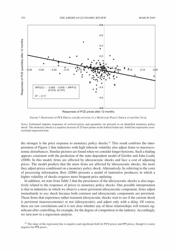
The right panel of Figure 4 represents the impulse responses of the PCE quantities to the same monetary policy shock. While on average the real consumption responses tend to fall subsequent to the monetary shock, before reverting to the initial level, there is considerable variation across sectors. As for the price responses, the average real consumption responses display some persis-tence. Interestingly, sectors in which prices fall the most following a monetary shock tend to be sectors in which quantities fall the least, as indicated in Figure 7. This figure displays the scatter plot across PCE categories of the responses of prices and quantities 12 months after the monetary shock, and the regression line reveals a significant and negative slope.
To the extent that one is interested in characterizing the behavior of the economy in response to monetary policy actions, our results provide empirical support for features such as price rigidi-ties and inflation persistence often embedded in monetary models. Our findings, however, con-trast sharply with those of Bils, Klenow, and Kryvtsov (2003) and Balke and Wynne (2007), which call for a rejection of conventional sticky-price models. These authors found the opposite conclusion, mainly because they estimate an important price puzzle.
Bils, Klenow, and Kryvtsov (2003) estimate responses of 123 components of the CPI to fed-eral funds rate innovations, where the innovations are extracted from a seven-variable monthly VAR. As the VAR is estimated independently from the disaggregated price data, the responses obtained constitute only rough estimates of the price responses. Based on frequencies of price adjustments reported in Bils and Klenow (2004), they consider two categories of price respons-es—the flexible price and sticky price categories—and they report the responses of the prices in both categories as well as their ratio. They argue that the movements in relative prices are incon-sistent with a popular sticky-price model. Following an expansionary monetary policy shock, their estimated relative price (of flexible prices relative to sticky prices) declines initially and then increases, while in the model, the relative price increases temporarily before reverting back to zero. However, the main reason for their finding of an unconventional relative price response in the data is related to the fact that their estimates of flexible-price responses display a price puzzle: flexible prices fall initially in response to a monetary policy expansion, and increase only later. In contrast, sticky prices do not show significant dynamics in the first 20 months.
Balke and Wynne (2007) focus instead on components of the PPI. After estimating a small-sized VAR and the response of components of the PPI to an identified monetary policy shock, they also find a substantial price puzzle in individual series, and thus conclude, as do Bils, Klenow, and Kryvtsov (2003), that the estimated evolution of relative prices is inconsistent with the evolution predicted by sticky-price models.
These studies make two key assumptions about the behavior of the macroeconomy: (i) that the macroeconomic dynamics can be properly uncovered from a small set of macroeconomic indicators, and (ii) that macroeconomic dynamics can be modeled separately from the disag-gregated prices. Based on the results of BBE, and as argued above, the first assumption does not seem to be empirically valid and could be responsible for finding a price puzzle. The second assumption implies that disaggregated prices have an effect on the macroeconomy only through an observed aggregate index. The FAVAR framework that we consider in this paper relaxes these two assumptions, as it allows us to incorporate more information in the estimation of the
VOL. 99 NO. 1 369BOiViN ET AL.: STicky PRicES ANd MONETARy POLicy
macroeconomic dynamics, and to model the disaggregated dynamics in a more flexible fash-ion. Interestingly, in contrast to these studies, we don’t find any evidence of price puzzle in our estimated FAVAR. This implies that the ratio of flexible to sticky prices behaves as predicted by standard monetary models (including sticky-price models), with flexible prices falling after a contractionary monetary policy shock.
C. cross-Sectional Variation in Price Responses
Having estimated impulse responses of sectoral prices to monetary policy shocks, we now attempt to explain differences in price responses with sectoral characteristics.
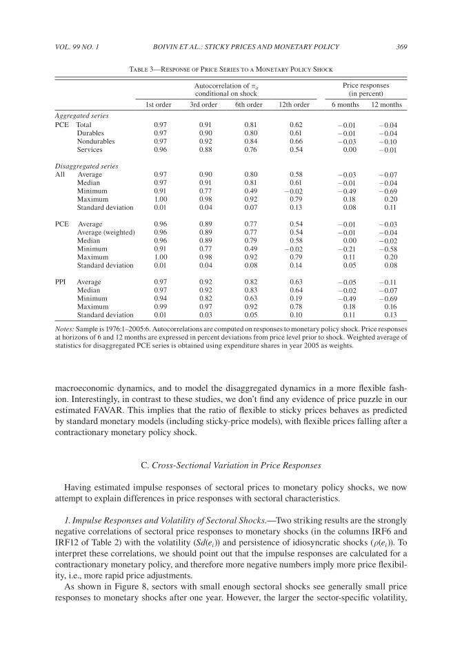
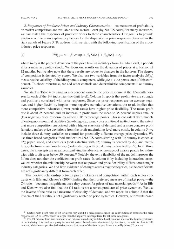
1. impulse Responses and Volatility of Sectoral Shocks.—Two striking results are the strongly negative correlations of sectoral price responses to monetary shocks (in the columns IRF6 and IRF12 of Table 2) with the volatility (Sd(ei )) and persistence of idiosyncratic shocks (ρ(ei )). To interpret these correlations, we should point out that the impulse responses are calculated for a contractionary monetary policy, and therefore more negative numbers imply more price flexibil-ity, i.e., more rapid price adjustments.
As shown in Figure 8, sectors with small enough sectoral shocks see generally small price responses to monetary shocks after one year. However, the larger the sector-specific volatility,
Table 3—Response of Price Series to a Monetary Policy Shock
Autocorrelation of πit Price responsesconditional on shock (in percent)
1st order 3rd order 6th order 12th order 6 months 12 months
Aggregated seriesPCE Total 0.97 0.91 0.81 0.62 −0.01 −0.04 Durables 0.97 0.90 0.80 0.61 −0.01 −0.04 Nondurables 0.97 0.92 0.84 0.66 −0.03 −0.10 Services 0.96 0.88 0.76 0.54 0.00 −0.01
disaggregated seriesAll Average 0.97 0.90 0.80 0.58 −0.03 −0.07 Median 0.97 0.91 0.81 0.61 −0.01 −0.04 Minimum 0.91 0.77 0.49 −0.02 −0.49 −0.69 Maximum 1.00 0.98 0.92 0.79 0.18 0.20 Standard deviation 0.01 0.04 0.07 0.13 0.08 0.11
PCE Average 0.96 0.89 0.77 0.54 −0.01 −0.03 Average (weighted) 0.96 0.89 0.77 0.54 −0.01 −0.04 Median 0.96 0.89 0.79 0.58 0.00 −0.02 Minimum 0.91 0.77 0.49 −0.02 −0.21 −0.58 Maximum 1.00 0.98 0.92 0.79 0.11 0.20 Standard deviation 0.01 0.04 0.08 0.14 0.05 0.08
PPI Average 0.97 0.92 0.82 0.63 −0.05 −0.11 Median 0.97 0.92 0.83 0.64 −0.02 −0.07 Minimum 0.94 0.82 0.63 0.19 −0.49 −0.69 Maximum 0.99 0.97 0.92 0.78 0.18 0.16 Standard deviation 0.01 0.03 0.05 0.10 0.11 0.13
Notes: Sample is 1976:1–2005:6. Autocorrelations are computed on responses to monetary policy shock. Price responses at horizons of 6 and 12 months are expressed in percent deviations from price level prior to shock. Weighted average of statistics for disaggregated PCE series is obtained using expenditure shares in year 2005 as weights.
MARch 2009370 ThE AMERicAN EcONOMic REViEW
the stronger is the price response to monetary policy shocks.23 This result confirms the inter-pretation of Figure 1 that industries with high inherent volatility also adjust faster to macroeco-nomic disturbances. Similar pictures are found when we consider longer horizons. Such a finding appears consistent with the prediction of the state-dependent model of Gertler and John Leahy (2008). In this model, firms are affected by idiosyncratic shocks and face a cost of adjusting prices. The model predicts that the more firms are affected by idiosyncratic shocks, the more they adjust prices conditional on a monetary policy shock. Alternatively, by referring to the costs of processing information, Reis (2006) presents a model of inattentive producers in which a higher volatility of shocks requires more frequent price updating.
In addition, we note from Table 2 that the persistence of the idiosyncratic shocks is also nega-tively related to the responses of prices to monetary policy shocks. One possible interpretation is that in industries in which we observe a more persistent idiosyncratic component, firms adjust immediately to any shock because both common and idiosyncratic components are persistent. Those firms that experience rather transient idiosyncratic shocks wait to see if the current shock is persistent (macroeconomic) or not (idiosyncratic), and adjust only with a delay. Of course, these are raw correlations and it is not clear whether any of these relationships will remain sig-nificant after controlling, for example, for the degree of competition in the industry. Accordingly, we turn now to a regression analysis.
23 The slope of the regression line is negative and significant both for PCE prices and PPI prices, though it is more negative for PPI prices.
Figure 7. Responses of PCE Prices and Quantities to a Monetary Policy Shock after One Year
Notes: Estimated impulse responses of sectoral prices and quantities (in percent) to an identified monetary policy shock. The monetary shock is a surprise increase of 25 basis points in the federal funds rate. Solid line represents cross-sectional regression line.
−0.8
−0.6
−0.4
−0.2
0
0.2
0.4
0.6
−0.30 −0.25 −0.20 −0.15 −0.10 −0.05 0.00 0.05 0.10 0.15 0.20
Responses of PCE prices after 12 months
Res
pons
es o
f PC
E q
uant
ities
afte
r 12
mon
ths
0.8
IRFQ12 = −0.083 − 0.678 × IRFP12 (0.010) (0.107)
R2 = 0.17
VOL. 99 NO. 1 371BOiViN ET AL.: STicky PRicES ANd MONETARy POLicy
2. Responses of Producer Prices and industry characteristics.—As measures of profitability or market competition are available at the sectoral level (by NAICS codes) for many industries, we can match the responses of producer prices to these characteristics. Our goal is to provide evidence on the main explanatory factors for the dispersion in price responses observed in the right panels of Figure 3. To address this, we start with the following specification of the cross-industry price responses:
(4) iRFi,h = a + β1 compi + β2 Sd(ei ) + β3 ρ(ei ) + εi,
where iRFi,h is the percent deviation of the price level in industry i from its initial level, h periods after a monetary policy shock. We focus our results on the deviation of prices at a horizon of 12 months, but we also note that these results are robust to changes in the horizon. The degree of competition is denoted by compi. We also use two variables from the factor analysis: Sd(ei) measures the volatility of the idiosyncratic component, while ρ(ei) is the persistence of this com-ponent. To check robustness, we add other controls and deterministic components like dummy variables.
We start in Table 4 by using as a dependent variable the price response at the 12-month hori-zon for each of the 149 industries (six-digit level). Column 1 reports that profit rates are strongly and positively correlated with price responses. Since our price responses are on average nega-tive, and higher flexibility implies more negative cumulative deviations, the result implies that more competitive industries (lower profit rates) have higher price flexibility. The mean profit rate is about 25 percent, and an increase in profit from the mean to 35 percent implies smaller (less negative) price response by almost 0.05 percentage points. This is consistent with models of endogenous nominal rigidities (involving, e.g., menu costs or rational inattention) to the extent that more competition, associated with a higher elasticity of demand and a more concave profit function, makes price deviations from the profit-maximizing level more costly. In column 5, we include three dummy variables to control for potentially different average price dynamics. We use three broad categories: food and textiles (NAICS codes starting with 31; dummy is coded as d1); paper, wood, and chemicals (codes starting with 32; dummy is denoted by d2); and metal-lurgy, electronics, and machinery (codes starting with 33; dummy is denoted by d3). In all three cases, the intercepts are negative, signifying the absence, on average, of a price puzzle for indus-tries with profit rates below 50 percent.24 Notably, the extra flexibility of the model improves the fit but does not alter the coefficient on profit rates. In column 6, by including interaction terms, we test whether the relationship between market power and price flexibility differs across major industry categories. We find little evidence of changes across major categories, as the coefficients are not significantly different from each other.
This positive relationship between price stickiness and competition within each sector con-trasts with Bils and Klenow’s (2004) finding that their preferred measure of market power—the C4 ratio—becomes insignificant once they control for prices of raw material goods.25 As in Bils and Klenow, we also find that the C4 ratio is not a robust predictor of price dynamics. We use the inverse of the ratio as a measure of elasticity of demand, and we report in column 2 that the inverse of the C4 ratio is not significantly related to price dynamics. However, our results based
24 Sectors with profit rates of 0.5 or larger may exhibit a price puzzle, since the contribution of profits to the price responses is 0.5 × 0.493, which is larger than the negative intercept term for all three categories.
25 The C4 ratio (or four-firm concentration ratio) of an industry is defined as the market share of the four largest firms in the industry. It is used as a proxy for market power. In industries dominated by few firms, the ratio is close to 100 percent, while in competitive industries the market share of the four largest firms is usually below 20 percent.
MARch 2009372 ThE AMERicAN EcONOMic REViEW
on mean profit rates imply that for producer prices, market power is robustly related to price dynamics in response to monetary shocks.
Columns 3 and 4 confirm the observations from the correlation matrix (Table 2): both idiosyn-cratic volatility and persistence are negatively related to price impulse responses. This implies that firms in industries with persistent and volatile idiosyncratic shocks adjust rapidly to changes in the macroeconomic environment. Interestingly, the result survives once we include as controls profit rates (column 7). We will treat the specification in column 7 as our baseline in order to explore the robustness of our findings. The last column of Table 4 shows that gross profit rates and idiosyncratic volatility are also significant predictors of price flexibility at the six-month horizon.
To sum up, our sectoral analysis indicates that as predicted by models based on monopolistic competition, prices adjust more sluggishly in industries in which market power is higher. In addi-tion, we uncovered two other important determinants of price responses: idiosyncratic volatility and the persistence of industry-specific shocks.
D. Evidence of Relative-Price changes
One characteristic of the sectoral price and quantity responses reported in Figures 3 and 4 is that they seem to imply important degrees of long-run monetary nonneutrality. In fact, following a monetary shock, the price responses do not all converge to the same level, at least in the first
−0.6
−0.5
−0.4
−0.3
−0.2
−0.1
0
0.1
0.2
0.3
0 2 4 6 8 10 12
Standard deviation of idiosyncratic components (ei)
Pric
e re
spon
ses
afte
r 12
mon
ths
PPI
PCE
IRF12 = −0.022 − 0.043 × Sd(ei) (0.008) (0.005) R2 = 0.19
Figure 8. Price Responses to Monetary Shocks after One Year and Volatility of Sector-Specific Components
Notes: Estimated impulse responses of sectoral prices to identified monetary policy shock are expressed in percent. The monetary shock is a surprise increase of 25 basis points in the federal funds rate. Solid line represents cross-sec-tional regression line.
VOL. 99 NO. 1 373BOiViN ET AL.: STicky PRicES ANd MONETARy POLicy
four years following the shock.26 It is important to realize, however, that the long-run responses to a monetary policy shock obtained from such analysis tend to be quite imprecisely estimated. We thus investigate whether there is in fact evidence of long-run relative price changes follow-ing monetary shocks, once the uncertainty surrounding the estimated responses is taken into account.
To account explicitly for the uncertainty surrounding the responses of relative prices, we use the empirical distribution of each sector’s impulse response functions to a monetary shock, under the null hypothesis that at a given (long-run) horizon all price responses reach the same level. More precisely, for each of the sectoral price series, we impose the restriction that the response must be equal to the aggregate price response at the horizon of four years or ten years after the shock. Such restrictions involve only the factor loadings Λ in the observation equation (2), and for each price series, the coefficients in the observation equation are estimated via restricted OLS. Appendix A contains technical details about this estimation and presents the least-squares estimator of the factor loadings.27 The empirical distribution is obtained through the bootstrap procedure described in footnote 10.28 For any given sector, we test for the long-run equality of sectoral price responses by determining whether the unrestricted impulse response function falls into the confidence region of the constrained response. Under the null hypothesis that there are no long-run relative price changes, we would expect that 10 percent of the sectors would display significant relative price changes at the 10 percent confidence level. In fact, less than 1 percent of the PCE and PPI sectors reveal relative price changes at that confidence level, four years or ten years following the monetary shock. Thus, we cannot reject the hypothesis that the long-run sectoral price responses are the same as the response of the aggregate price index.
It is certainly possible that this test fails to reject the long-run homogeneity of the price re- sponses because of the imprecision of our estimates. One might, thus, still be concerned that the cross-sectional regression results reported in the previous section may be affected by the dispar-ity of long-run price responses. In particular, while we interpreted the results of Table 4 as sug-gesting that prices in sectors with more volatile idiosyncratic shocks respond faster to monetary shocks, an alternative interpretation is that sectors with volatile idiosyncratic shocks respond more to monetary policy shocks in the long run.
To determine which explanation is more likely, and to assess the effect of the apparent long-run relative price changes on these results, we repeat our cross-sectional regressions imposing the restriction that all price indices have a response to the monetary policy shock that is equal to the response of the aggregate price index in the long run. This ensures that there are no long-run effects of monetary policy on relative prices. We report results using our FAVAR estimated with long-run restrictions at a horizon of four and ten years. Figure 9 plots the responses of PCE and PPI prices to a monetary shock when these long-run restrictions are imposed. Table 5 provides the statistics reported in Table 3 when the restrictions are imposed. Apart from the fact that the price responses are by construction all equal to the response of the aggregate price index at some given horizon in the future, these results reveal no important difference with respect to the case discussed above. Table 6 provides further evidence that gross profit rates and idiosyncratic vola-tility are significant predictors of price flexibility. The results reported in columns 1–4 suggest
26 William D. Lastrapes (2006), using VARs, finds that productivity and money supply shocks have long-run effects on the distribution of relative commodity prices.
27 These restrictions are different from the long-run restrictions used to identify structural shocks (e.g., Olivier J. Blanchard and Danny Quah 1989). We chose to impose the constraints on the loading matrix Λ, as it is more likely that the dispersion in long-run responses reflects sample uncertainty related to factor loadings than to the identification of policy shocks. Nonetheless, it will be interesting, in future work, to study the effects of structural shocks identified through long-run restrictions in FAVAR models.
28 The bootstrapped impulse responses involve 10,000 iterations.
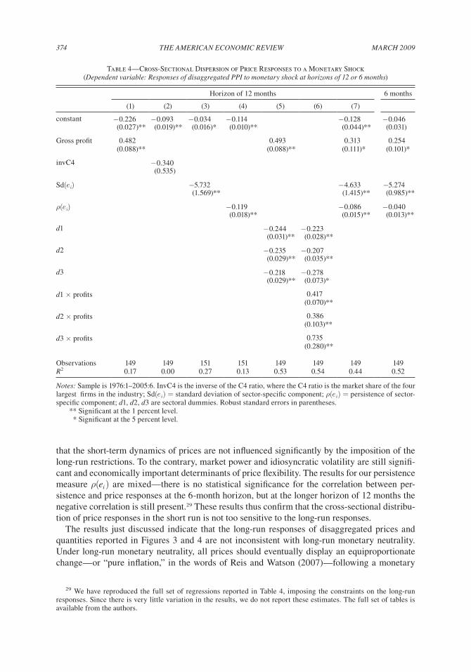
MARch 2009374 ThE AMERicAN EcONOMic REViEW
that the short-term dynamics of prices are not influenced significantly by the imposition of the long-run restrictions. To the contrary, market power and idiosyncratic volatility are still signifi-cant and economically important determinants of price flexibility. The results for our persistence measure ρ(ei ) are mixed—there is no statistical significance for the correlation between per-sistence and price responses at the 6-month horizon, but at the longer horizon of 12 months the negative correlation is still present.29 These results thus confirm that the cross-sectional distribu-tion of price responses in the short run is not too sensitive to the long-run responses.
The results just discussed indicate that the long-run responses of disaggregated prices and quantities reported in Figures 3 and 4 are not inconsistent with long-run monetary neutrality. Under long-run monetary neutrality, all prices should eventually display an equiproportionate change—or “pure inflation,” in the words of Reis and Watson (2007)—following a monetary
29 We have reproduced the full set of regressions reported in Table 4, imposing the constraints on the long-run responses. Since there is very little variation in the results, we do not report these estimates. The full set of tables is available from the authors.
Table 4—Cross-Sectional Dispersion of Price Responses to a Monetary Shock (dependent variable: Responses of disaggregated PPi to monetary shock at horizons of 12 or 6 months)
Horizon of 12 months 6 months
(1) (2) (3) (4) (5) (6) (7)
constant −0.226 −0.093 −0.034 −0.114 −0.128 −0.046(0.027)** (0.019)** (0.016)* (0.010)** (0.044)** (0.031)
Gross profit 0.482 0.493 0.313 0.254(0.088)** (0.088)** (0.111)* (0.101)*
invC4 −0.340(0.535)
Sd(ei) −5.732 −4.633 −5.274(1.569)** (1.415)** (0.985)**
ρ(ei) −0.119 −0.086 −0.040(0.018)** (0.015)** (0.013)**
d1 −0.244 −0.223(0.031)** (0.028)**
d2 −0.235 −0.207(0.029)** (0.035)**
d3 −0.218 −0.278(0.029)** (0.073)*
d1 × profits 0.417(0.070)**
d2 × profits 0.386(0.103)**
d3 × profits 0.735(0.280)**
Observations 149 149 151 151 149 149 149 149R2 0.17 0.00 0.27 0.13 0.53 0.54 0.44 0.52
Notes: Sample is 1976:1–2005:6. InvC4 is the inverse of the C4 ratio, where the C4 ratio is the market share of the four largest firms in the industry; Sd(ei) = standard deviation of sector-specific component; ρ(ei) = persistence of sector-specific component; d1, d2, d3 are sectoral dummies. Robust standard errors in parentheses.
** Significant at the 1 percent level. * Significant at the 5 percent level.
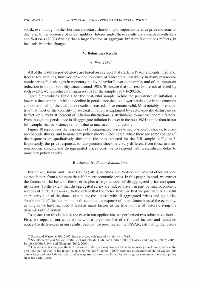
VOL. 99 NO. 1 375BOiViN ET AL.: STicky PRicES ANd MONETARy POLicy
shock, even though in the short run monetary shocks imply important relative price movements due, e.g., to the presence of price rigidities. Interestingly, these results are consistent with Reis and Watson’s (2007) finding that a large fraction of aggregate inflation fluctuations reflects, in fact, relative price changes.
V. Robustness Results
A. Post-1984
All of the results reported above are based on a sample that starts in 1976:1 and ends in 2005:6. Recent research has, however, provided evidence of widespread instability in many macroeco-nomic series,30 of changes in monetary policy behavior 31 over our sample, and of an important reduction in output volatility since around 1984. To ensure that our results are not affected by such events, we reproduce our main results for the sample 1984:1–2005:6.
Table 7 reproduces Table 1 for the post-1984 sample. While the persistence in inflation is lower in that sample—with the decline in persistence due to a lower persistence in the common component—all of the qualitative results discussed above remain valid. Most notably, it remains true that most of the volatility in sectoral inflation is explained by sector-specific disturbances. In fact, only about 10 percent of inflation fluctuations is attributable to macroeconomic factors. Even though the persistence in disaggregate inflation is lower in the post-1984 sample than in our full sample, that persistence remains due to macroeconomic factors.
Figure 10 reproduces the responses of disaggregated prices to sector-specific shocks, to mac-roeconomic shocks, and to monetary policy shocks. Once again, while there are some changes,32 the responses are qualitatively similar to the ones reported for the full sample in Figure 3. Importantly, the price responses to idiosyncratic shocks are very different from those to mac-roeconomic shocks, and disaggregated prices continue to respond with a significant delay to monetary policy shocks.
B. Alternative Factor Estimations
Bernanke, Boivin, and Eliasz (2005) (BBE), as Stock and Watson and several other authors, extract factors from a bit more than 100 macroeconomic series. In this paper, instead, we extract the factors on the basis of these series plus a large number of disaggregated price and quan-tity series. To the extent that disaggregated series are indeed driven in part by macroeconomic sources of fluctuations—i.e., to the extent that the factor structure that we postulate is a useful characterization of the data—expanding the dataset with disaggregated prices and quantities should not “tilt” the factors in one direction at the expense of other dimensions of the economy, as long as we have included at least as many factors as the true number of factors driving the dynamics of the system.
To ensure that this is indeed the case in our application, we performed two robustness checks. First, we repeated our calculations with a larger number of estimated factors, and found no noticeable differences in our results. Second, we reestimated the FAVAR, estimating the factors
30 Stock and Watson (1996, 2002) have provided evidence of instability in VARs.31 See Bernanke and Mihov (1998); Richard Clarida, Galí, and Gertler (2000); Cogley and Sargent (2002, 2005);
Boivin (2006); Boivin and Giannoni (2002, 2006).32 One noticeable change is the fact that overall, the price responses to the same monetary shock are smaller in the
post-1984 period than in the larger sample. Boivin and Giannoni (2006) estimate a structural model to explain this observation and conclude that the smaller responses are well explained by a change in systematic monetary policy since the early 1980s.
MARch 2009376 ThE AMERicAN EcONOMic REViEW
in the first stage only on the basis of the 111 series that were identified by Stock and Watson as the most informative series for extracting common factors. The extracted factors correspond to those used in BBE. We find that none of our conclusions is sensitive to this change in the infor-mation set.33
33 Table B.1 in online Appendix B repeats the calculations underlying Tables 1 and 3, this time estimating the latent factors on the smaller dataset. Overall, the results are almost identical for both sets of latent factors. One noticeable
0 12 24 36 48−1.5
−1
−0.5
0
0.5
PCE (restrictions: 4 years)
0 12 24 36 48−1
−0.5
0
0.5
PPI (restrictions: 4 years)
0 12 24 36 48−1.5
−1
−0.5
0
0.5
PCE (restrictions: 10 years)
0 12 24 36 48−1
−0.5
0
0.5
PPI (restrictions: 10 years)
Figure 9. Sectoral Price Responses to Monetary Shocks with Long-Run Restrictions at Horizon of Four and Ten Years
Notes: Estimated impulse responses of sectoral prices (in percent) to an identified monetary policy shock. The mon-etary shock is a surprise increase of 25 basis points in the federal funds rate. Thick solid lines represent unweighted average responses. Thick dashed lines represent the response of the aggregate PCE and PPI (finished) price indices to a monetary policy shock. In left panels, all price responses are constrained to be equal to the aggregate price response at the horizon of four years. In right panels, the constraints apply at the horizon of ten years.
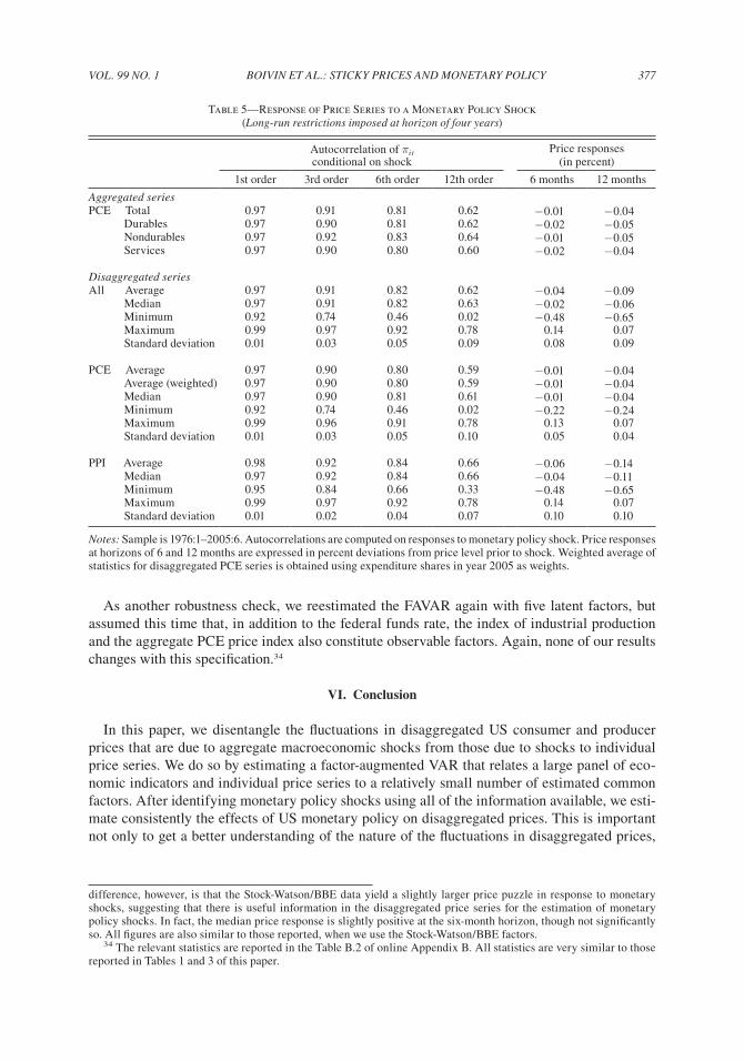
VOL. 99 NO. 1 377BOiViN ET AL.: STicky PRicES ANd MONETARy POLicy
As another robustness check, we reestimated the FAVAR again with five latent factors, but assumed this time that, in addition to the federal funds rate, the index of industrial production and the aggregate PCE price index also constitute observable factors. Again, none of our results changes with this specification.34
VI. Conclusion
In this paper, we disentangle the fluctuations in disaggregated US consumer and producer prices that are due to aggregate macroeconomic shocks from those due to shocks to individual price series. We do so by estimating a factor-augmented VAR that relates a large panel of eco-nomic indicators and individual price series to a relatively small number of estimated common factors. After identifying monetary policy shocks using all of the information available, we esti-mate consistently the effects of US monetary policy on disaggregated prices. This is important not only to get a better understanding of the nature of the fluctuations in disaggregated prices,
difference, however, is that the Stock-Watson/BBE data yield a slightly larger price puzzle in response to monetary shocks, suggesting that there is useful information in the disaggregated price series for the estimation of monetary policy shocks. In fact, the median price response is slightly positive at the six-month horizon, though not significantly so. All figures are also similar to those reported, when we use the Stock-Watson/BBE factors.
34 The relevant statistics are reported in the Table B.2 of online Appendix B. All statistics are very similar to those reported in Tables 1 and 3 of this paper.
Table 5—Response of Price Series to a Monetary Policy Shock (Long-run restrictions imposed at horizon of four years)
Autocorrelation of πi t Price responsesconditional on shock (in percent)
1st order 3rd order 6th order 12th order 6 months 12 months
Aggregated seriesPCE Total 0.97 0.91 0.81 0.62 −0.01 −0.04 Durables 0.97 0.90 0.81 0.62 −0.02 −0.05 Nondurables 0.97 0.92 0.83 0.64 −0.01 −0.05 Services 0.97 0.90 0.80 0.60 −0.02 −0.04
disaggregated seriesAll Average 0.97 0.91 0.82 0.62 −0.04 −0.09 Median 0.97 0.91 0.82 0.63 −0.02 −0.06 Minimum 0.92 0.74 0.46 0.02 −0.48 −0.65 Maximum 0.99 0.97 0.92 0.78 0.14 0.07 Standard deviation 0.01 0.03 0.05 0.09 0.08 0.09
PCE Average 0.97 0.90 0.80 0.59 −0.01 −0.04 Average (weighted) 0.97 0.90 0.80 0.59 −0.01 −0.04 Median 0.97 0.90 0.81 0.61 −0.01 −0.04 Minimum 0.92 0.74 0.46 0.02 −0.22 −0.24 Maximum 0.99 0.96 0.91 0.78 0.13 0.07 Standard deviation 0.01 0.03 0.05 0.10 0.05 0.04
PPI Average 0.98 0.92 0.84 0.66 −0.06 −0.14 Median 0.97 0.92 0.84 0.66 −0.04 −0.11 Minimum 0.95 0.84 0.66 0.33 −0.48 −0.65 Maximum 0.99 0.97 0.92 0.78 0.14 0.07 Standard deviation 0.01 0.02 0.04 0.07 0.10 0.10
Notes: Sample is 1976:1–2005:6. Autocorrelations are computed on responses to monetary policy shock. Price responses at horizons of 6 and 12 months are expressed in percent deviations from price level prior to shock. Weighted average of statistics for disaggregated PCE series is obtained using expenditure shares in year 2005 as weights.
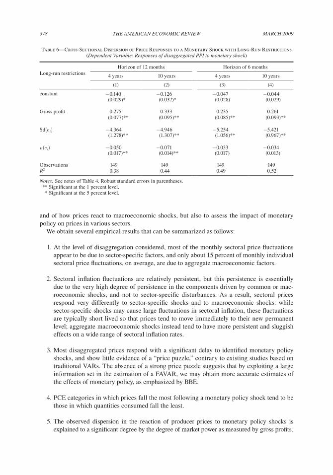
MARch 2009378 ThE AMERicAN EcONOMic REViEW
and of how prices react to macroeconomic shocks, but also to assess the impact of monetary policy on prices in various sectors.
We obtain several empirical results that can be summarized as follows:
1. At the level of disaggregation considered, most of the monthly sectoral price fluctuations appear to be due to sector-specific factors, and only about 15 percent of monthly individual sectoral price fluctuations, on average, are due to aggregate macroeconomic factors.
2. Sectoral inflation fluctuations are relatively persistent, but this persistence is essentially due to the very high degree of persistence in the components driven by common or mac-roeconomic shocks, and not to sector-specific disturbances. As a result, sectoral prices respond very differently to sector-specific shocks and to macroeconomic shocks: while sector-specific shocks may cause large fluctuations in sectoral inflation, these fluctuations are typically short lived so that prices tend to move immediately to their new permanent level; aggregate macroeconomic shocks instead tend to have more persistent and sluggish effects on a wide range of sectoral inflation rates.
3. Most disaggregated prices respond with a significant delay to identified monetary policy shocks, and show little evidence of a “price puzzle,” contrary to existing studies based on traditional VARs. The absence of a strong price puzzle suggests that by exploiting a large information set in the estimation of a FAVAR, we may obtain more accurate estimates of the effects of monetary policy, as emphasized by BBE.
4. PCE categories in which prices fall the most following a monetary policy shock tend to be those in which quantities consumed fall the least.
5. The observed dispersion in the reaction of producer prices to monetary policy shocks is explained to a significant degree by the degree of market power as measured by gross profits.
Table 6—Cross-Sectional Dispersion of Price Responses to a Monetary Shock with Long-Run Restrictions (dependent Variable: Responses of disaggregated PPi to monetary shock)
Horizon of 12 months Horizon of 6 monthsLong-run restrictions 4 years 10 years 4 years 10 years
(1) (2) (3) (4)
constant −0.140 −0.126 −0.047 −0.044(0.029)* (0.032)* (0.028) (0.029)
Gross profit 0.275 0.333 0.235 0.261(0.077)** (0.095)** (0.085)** (0.093)**
Sd(ei) −4.364 −4.946 −5.254 −5.421(1.278)** (1.307)** (1.056)** (0.967)**
ρ(ei) −0.050 −0.071 −0.033 −0.034(0.017)** (0.014)** (0.017) (0.013)
Observations 149 149 149 149R2 0.38 0.44 0.49 0.52
Notes: See notes of Table 4. Robust standard errors in parentheses. ** Significant at the 1 percent level. * Significant at the 5 percent level.
VOL. 99 NO. 1 379BOiViN ET AL.: STicky PRicES ANd MONETARy POLicy
6. Prices react more rapidly to monetary policy shocks in sectors with volatile idiosyncratic and persistent idiosyncratic shocks.
7. The correlations between the idiosyncratic components of prices and quantities tend to be negative, suggesting that sector-specific shocks may be driven by supply-type shocks, and/or may reflect sampling error in measured disaggregated prices.
This collection of stylized facts regarding the response of disaggregated US prices to various shocks presents challenges to current models of price determination. An evaluation of various models on the basis of these stylized facts is beyond the scope of this paper. Nevertheless, it is worth pointing out that our finding number 2—namely that sectoral prices respond differently to macroeconomic and sector-specific shocks—may explain why sticky-price models such as the Calvo model have been so popular in characterizing the effects of monetary policy actions on aggregate variables, while they have been sharply criticized at the same time by authors focused on disaggregated price series.
Clearly, it would be desirable to have models that can fully account for the responses of aggre-gate and disaggregated prices to both macroeconomic and sector-specific disturbances. Some recent papers are very promising in this respect. Among models in which price setting is time dependent, Carvalho (2006) generalizes the Calvo model to allow for heterogeneity in price stickiness across sectors. He finds that, in the presence of strategic complementarities, firms that
Table 7—Volatility and Persistence of Monthly Inflation Series, Post-1984 sample
Standard deviation (in percent) Persistence
Common Sector- Common Sector-Inflation components specific R2 Inflation components specific
Aggregated seriesPCE Total 0.16 0.13 0.09 0.70 0.74 0.83 0.34 Durables 0.26 0.16 0.20 0.39 0.83 0.95 0.41 Nondurables 0.40 0.33 0.22 0.71 0.28 0.70 0.49 Services 0.16 0.09 0.13 0.30 0.73 0.96 −0.51
disaggregated seriesAll Average 0.97 0.25 0.93 0.10 0.23 0.86 −0.16 Median 0.64 0.16 0.62 0.07 0.30 0.88 −0.10 Minimum 0.11 0.02 0.10 0.00 −4.33 0.34 −2.35 Maximum 7.32 2.85 7.15 0.75 1.22 0.97 0.77 Standard deviation 0.98 0.30 0.94 0.11 0.49 0.08 0.49
PCE Average 0.86 0.24 0.81 0.13 0.19 0.87 −0.22 Average (weighted) 0.75 0.28 0.68 0.20 0.37 0.89 −0.08 Median 0.57 0.15 0.55 0.08 0.27 0.90 −0.21 Minimum 0.11 0.04 0.10 0.01 −4.33 0.49 −2.35 Maximum 7.32 2.85 7.15 0.75 0.95 0.97 0.77 Standard deviation 0.93 0.34 0.88 0.14 0.57 0.08 0.51
PPI Average 1.11 0.27 1.07 0.08 0.27 0.85 −0.10 Median 0.75 0.17 0.72 0.06 0.34 0.87 −0.02 Minimum 0.24 0.02 0.23 0.00 −1.32 0.34 −1.64 Maximum 6.34 1.49 6.29 0.33 1.22 0.96 0.77 Standard deviation 1.01 0.24 0.99 0.06 0.37 0.08 0.44
Notes: Sample is 1984:1–2005:6. Inflation is measured as πit = pit − pit − 1, where pit is the log of the price series i. Common components are λ′iCt; sector-specific components are eit. R
2 statistics measure the fraction of the variance of πit explained by λ′iCt; persistence is based on estimated AR processes with 13 lags. Weighted average of statistics for disaggregated PCE series is obtained using expenditure shares in year 2005 as weights.
MARch 2009380 ThE AMERicAN EcONOMic REViEW
adjust prices infrequently have a disproportionately large effect on the decisions of other firms, and thus on the aggregate price level. It would be interesting to study an extension of the multi-sector model in Carvalho (2006) with sectoral shocks. It may be the case that in this model prices respond quickly to sectoral shocks and slowly to monetary policy shocks.
Among state-dependent models, the menu-cost model of Golosov and Lucas (2007), which includes idiosyncratic productivity shocks but abstracts from strategic complementarities, gen-erates rapid and strong price responses following a monetary policy shock. Virgiliu Midrigan (2006), however, extends the model of Golosov and Lucas (2007) to a multiproduct setting and calibrates the distribution of idiosyncratic shocks in a way that mitigates the price responses to monetary shocks menu-cost models. Gertler and Leahy (2008) propose a state-dependent pricing model that involves volatile prices due to large idiosyncratic shocks, but that predicts sluggish price responses to a monetary shock, as reported here, due to real rigidities. Given that firms are assumed to consider price adjustments only when they are hit with sector-specific shocks, that model also predicts that a high volatility of idiosyncratic shocks should be associated with more volatile prices and a more volatile response to monetary shocks, as we find in the data.
0 12 24 36 48−15
−10
−5
0PCE: Sector-specific
0 12 24 36 48−10
−8
−6
−4
−2
0PPI: Sector-specific
0 12 24 36 48−15
−10
−5
0PCE: Common component
0 12 24 36 48−15
−10
−5
0PPI: Common component
0 12 24 36 48−3
−2
−1
0
1
2PCE: Monetary shock
0 12 24 36 48−3
−2
−1
0
1
2PPI: Monetary shock
Figure 10. Sectoral Price Responses to Various Shocks in Post-1984 Sample
Notes: Estimated impulse responses of sectoral prices (in %) to a sector-specific shock eit of one standard deviation (left panels), to a shock to the common component λ′iCt of one standard deviation (middle panels), and to an identified mon-etary policy shock (right panels). The monetary shock is a surprise increase of 25 basis points in the federal funds rate. Thick solid lines represent unweighted average responses. Thick dashed lines represent the response of the aggregate PCE and PPI (finished) price indices to a monetary policy shock.
VOL. 99 NO. 1 381BOiViN ET AL.: STicky PRicES ANd MONETARy POLicy
In yet another direction, Bartosz Mackowiak and Mirko Wiederholt (2007) present a model of rational inattention inspired by Sims (2003), which is also able to generate different responses of sectoral prices to sector-specific shocks and aggregate shocks. In such a model, prices may respond slowly to aggregate shocks but quickly to sector-specific shocks, as firms choose to pay relatively little attention to macroeconomic conditions and more attention to firm-specific conditions.35
Assessing the empirical success of each of these theories along the many dimensions docu-mented in this paper is not a trivial task. Even though a strict and literal interpretation of any of these models may always be rejected on some dimension, a fair assessment requires moving beyond the strict interpretation and determining whether some enriched version of existing theo-ries can be successful. In our view, this is an important avenue for future research.
Appendix A: Restrictions on Long-Run Responses to Monetary Shocks
Impulse responses for the price series are calculated by using the dynamics of the common factors and the following equation:
(5) Xit = λ′iCt + eit,
where Xit contains the monthly log change in the respective price series. The response of Xit after h periods is given by
Xi,h = λ′i Ch ,
where Ch is the vector of responses of the common factors after h periods. We want to impose the restriction that after h periods the response of the log price level in sector i is equal to a certain value denoted by a. We choose a to correspond to the response of the relevant aggregate price index. Since the price data are expressed in first differences, we cumulate the responses over the first h periods to obtain the log price level h periods after the shock. We thus impose the desired restrictions of the following form on the estimation of λi:
λ i ′ ∑
h=0
h
Ch = a.
Thus, we can estimate equation (5) by OLS subject to the restriction above.If we denote by λ i
u the unrestricted OLS estimate of the loadings, then the restricted least squares estimate of the loadings, λ i
r , can be calculated from the standard textbook formula (see, e.g., William H. Greene 2003, chap. 6, sect. 6.3.2):
λ i r = λ i
u − ( C t ′ Ct ) −1 a ∑ h=0
h
Ch b c a ∑ h=0
h
Ch b′ ( C t ′ Ct ) −1 a ∑
h=0
h
Ch b d −1
a λ i u′ ∑
h=0
h
Ch − ab .
Appendix B is available at http://www.aeaweb.org/articles.php?doi=10.1257/aer.99.1.350.
35 In the model of Reis (2006), firms rationally choose to be inattentive to news and occasionally update their infor-mation. This model predicts that (i) stickiness is higher in industries with low price elasticity of demand; (ii) costs of processing information are positively related with inattentiveness; and (iii) volatility of shocks requires more frequent updating. While this model does not distinguish between aggregate and sector-specific conditions, one can imagine an extension that would generate different responses to such shocks.
MARch 2009382 ThE AMERicAN EcONOMic REViEW
REFERENCES
Altissimo, Filippo, Benoît Mojon, and Paolo Zaffaroni. 2007. “Fast Micro and Slow Macro: Can Aggrega-tion Explain the Persistence of Inflation?” European Central Bank Working Paper 729.
Bai, Jushan. 2003. “Inferential Theory for Factor Models of Large Dimensions.” Econometrica, 71(1): 135–71.
Balke, Nathan S., and Mark A. Wynne. 2007. “The Relative Price Effects of Monetary Shocks.” Journal of Macroeconomics, 29(1): 19–36.
Bernanke, Ben S., and Alan S. Blinder. 1992. “The Federal Funds Rate and the Channels of Monetary Transmission.” American Economic Review, 82(4): 901–21.
Bernanke, Ben S., Jean Boivin, and Piotr Eliasz. 2005. “Measuring the Effects of Monetary Policy: A Fac-tor-Augmented Vector Autoregressive (FAVAR) Approach.” Quarterly Journal of Economics, 120(1): 387–422.
Bernanke, Ben S., and Ilian Mihov. 1998. “Measuring Monetary Policy.” Quarterly Journal of Econom-ics, 113(3): 869–902.
Bils, Mark, and Peter J. Klenow. 2004. “Some Evidence on the Importance of Sticky Prices.” Journal of Political Economy, 112(5): 947–85.
Bils, Mark, Peter J. Klenow, and Oleksiy Kryvtsov. 2003. “Sticky Prices and Monetary Policy Shocks.” Federal Reserve Bank of Minneapolis Quarterly Review, 27(1): 2–9.
Blanchard, Olivier J., and Danny Quah. 1989. “The Dynamic Effects of Aggregate Demand and Supply Disturbances.” American Economic Review, 79(4): 655–73.
Blinder, Alan S., Elie R. D. Canetti, David E. Lebow, and Jeremy B. Rudd. 1998. Asking about Prices: A New Approach to Understanding Price Stickiness. New York: Russell Sage Foundation.
Boivin, Jean. 2006. “Has U.S. Monetary Policy Changed? Evidence from Drifting Coefficients and Real-Time Data.” Journal of Money, credit, and Banking, 38(5): 1149–73.
Boivin, Jean, and Marc P. Giannoni. 2002. “Assessing Changes in the Monetary Transmission Mecha-nism: A VAR Approach.” Federal Reserve Bank of New york Economic Policy Review, 8(1): 97–11.
Boivin, Jean, and Marc P. Giannoni. 2006. “Has Monetary Policy Become More Effective?” Review of Economics and Statistics, 88(3): 445–62.
Boivin, Jean, Marc P. Giannoni, and Ilian Mihov. 2007. “Sticky Prices and Monetary Policy: Evidence from Disaggregated U.S. Data.” National Bureau of Economic Research Working Paper 12824.
Boivin, Jean, and Serena Ng. 2005. “Understanding and Comparing Factor-Based Forecasts.” interna-tional Journal of central Banking, 1(3): 117–51.
Broda, Christian, and David E. Weinstein. 2007. “Product Creation and Destruction: Evidence and Price Implications.” National Bureau of Economic Research Working Paper 13041.
Carlton, Dennis W. 1986. “The Rigidity of Prices.” American Economic Review, 76(4): 637–58.Carvalho, Carlos. 2006. “Heterogeneity in Price Stickiness and the Real Effects of Monetary Shocks.”
B E Journals in Macroeconomics: Frontiers of Macroeconomics, 2(1): 1–56.Cecchetti, Stephen G. 1986. “The Frequency of Price Adjustment: A Study of the Newsstand Prices of
Magazines.” Journal of Econometrics, 31(3): 255–74.Christiano, Lawrence J., Martin Eichenbaum, and Charles Evans. 1999. “Monetary Policy Shocks: What
Have We Learned and to What End?” In handbook of Macroeconomics, Volume 1A, ed. John B. Taylor and Michael Woodford, 65–148. New York: Elsevier Science.
Christiano, Lawrence J., Martin Eichenbaum, and Charles Evans. 2005. “Nominal Rigidities and the Dynamic Effects of a Shock to Monetary Policy.” Journal of Political Economy, 113(1): 1–45.
Clarida, Richard, Jordi Galí, and Mark Gertler. 2000. “Monetary Policy Rules and Macroeconomic Sta-bility: Evidence and Some Theory.” Quarterly Journal of Economics, 115(1): 147–80.
Clark, Todd E. 2006. “Disaggregate Evidence on the Persistence of Consumer Price Inflation.” Journal of Applied Econometrics, 21(5): 563–87.
Cogley, Timothy, and Thomas J. Sargent. 2002. “Evolving Post–World War II U.S. Inflation Dynamics.” In NBER Macroeconomics Annual 2001, ed. Ben S. Bernanke and Kenneth S. Rogoff, 331–73. Cam-bridge, MA: MIT Press.
Cogley, Timothy, and Thomas J. Sargent. 2005. “Drifts and Volatilities: Monetary Policies and Outcomes in the Post WWII US.” Review of Economic dynamics, 8(2): 262–302.
Franco, Francesco, and Thomas Philippon. 2007. “Firms and Aggregate Dynamics.” Review of Econom-ics and Statistics, 89(4): 587–600.
Fuhrer, Jeffrey C., and George R. Moore. 1995. “Inflation Persistence.” Quarterly Journal of Economics, 110(1): 127–59.
VOL. 99 NO. 1 383BOiViN ET AL.: STicky PRicES ANd MONETARy POLicy
Galí, Jordi, and Mark Gertler. 1999. “Inflation Dynamics: A Structural Econometric Analysis.” Journal of Monetary Economics, 44(2): 195–222.
Gertler, Mark, and John Leahy. 2008. “A Phillips Curve with an Ss Foundation.” Journal of Political Economy, 116(3): 533–72.
Golosov, Mikhail, and Robert E. Lucas, Jr. 2007. “Menu Costs and Phillips Curves.” Journal of Political Economy, 115(2): 171–99.
Granger, Clive. 1980. “Long Memory Relationships and the Aggregation of Dynamic Models.” Journal of Econometrics, 14(2): 227–38.
Greene, William H. 2003. Econometric Analysis. Upper Saddle River, NJ: Prentice Hall.Imbs, Jean, Haroon Mumtaz, Morten O. Ravn, and Hélène Rey. 2005. “PPP Strikes Back: Aggregation
and the Real Exchange Rate.” Quarterly Journal of Economics, 120(1): 1–43.Kackmeister, Alan. 2007. “Yesterday’s Bad Times Are Today’s Good Old Times: Retail Price Changes Are
More Frequent Today Than in the 1890s.” Journal of Money, credit, and Banking, 39(8): 1987–2020.Kashyap, Anil K. 1995. “Sticky Prices: New Evidence from Retail Catalogs.” Quarterly Journal of Eco-
nomics, 110(1): 245–74.Kilian, Lutz. 1998. “Small-Sample Confidence Intervals for Impulse Response Functions.” Review of Eco-
nomics and Statistics, 80(2): 218–30.Klenow, Peter J., and Oleksiy Kryvtsov. 2008. “State-Dependent or Time-Dependent Pricing: Does It Mat-
ter for Recent U.S. Inflation?” Quarterly Journal of Economics, 123(3): 863–904.Lastrapes, William D. 2006. “Inflation and the Distribution of Relative Prices: The Role of Productivity
and Money Supply Shocks.” Journal of Money, credit, and Banking, 38(8): 2159–98.Leeper, Eric, Christopher A. Sims, and Tao Zha. 1996. “What Does Monetary Policy Do?” Brookings
Papers on Economic Activity, 2: 1–63.Levin, Andrew T., and Jeremy Piger. 2003. “Is Inflation Persistence Intrinsic in Industrial Economies?”
Federal Reserve Bank of St. Louis Working Paper 2002–023.Levy, Daniel, Mark Bergen, Shantanu Dutta, and Robert Venable. 1997. “The Magnitude of Menu Costs:
Direct Evidence from Large U.S. Supermarket Chains.” Quarterly Journal of Economics, 112(3): 791–825.MacDonald, James M., and Daniel Aaronson. 2000. “How Do Retail Prices React to Minimum Wage
Increases?” Federal Reserve Bank of Chicago Working Paper WP–00–20.Ma�ckowiak, Bartosz A., and Mirko Wiederholt. 2007. “Optimal Sticky Prices under Rational Inattention.”
CEPR Discussion Paper 6243.Midrigan, Virgiliu. 2006. “Menu Costs, Multi-Product Firms, and Aggregate Fluctuations.” http://homep-
ages.nyu.edu/~vm50/multiproductfirms.pdf.Nakamura, Emi, and Jón Steinsson. 2008. “Five Facts About Prices: A Reevaluation of Menu Cost Mod-
els.” Quarterly Journal of Economics, 123(4): 1415–64.Pesaran, M. Hashem, and Ron Smith. 1995. “Estimating Long-Run Relationships from Dynamic Hetero-
geneous Panels.” Journal of Econometrics, 68(1): 79–113.Pivetta, Frederic, and Ricardo Reis. 2007. “The Persistence of Inflation in the United States.” Journal of
Economic dynamics and control, 31(4): 1326–58.Reis, Ricardo. 2006. “Inattentive Producers.” Review of Economic Studies, 73(3): 793–821.Reis, Ricardo, and Mark W. Watson. 2007. “Relative Goods’ Prices and Pure Inflation.” National Bureau
of Economic Research Working Paper 13615.Rotemberg, Julio J., and Michael Woodford. 1997. “An Optimization-Based Econometric Framework for
the Evaluation of Monetary Policy.” In NBER Macroeconomics Annual 1997, ed. Ben S. Bernanke and Julio J. Rotemberg, 297–346. Cambridge, MA: MIT Press.
Shoemaker, Owen J. 2006. “Variance Estimates for Price Changes in the Consumer Price Index, January 2006–December 2006.” http://www.bls.gov/cpi/cpivar2006.pdf.
Sims, Christopher A. 1992. “Interpreting the Macroeconomic Time Series Facts: The Effects of Monetary Policy.” European Economic Review, 36(5): 975–1000.
Sims, Christopher A. 2002. “Comment: Evolving Post–World War II U.S. Inflation Dynamics.” In NBER Macroeconomics Annual 2001, ed. Ben S. Bernanke and Kenneth Rogoff, 373–79. Cambridge, MA: MIT Press.
Sims, Christopher A. 2003. “Implications of Rational Inattention.” Journal of Monetary Economics, 50(3): 665–90.
Smets, Frank, and Raf Wouters. 2007. “Shocks and Frictions in US Business Cycles: A Bayesian DSGE Approach.” American Economic Review, 97(3): 586–606.
Stock, James H. 2002. “Comment: Evolving Post–World War II U.S. Inflation Dynamics.” In NBER Mac-roeconomics Annual 2001, ed. Ben S. Bernanke and Kenneth S. Rogoff, 379–387. Cambridge, MA: MIT Press.

MARch 2009384 ThE AMERicAN EcONOMic REViEW
Stock, James H., and Mark W. Watson. 1996. “Evidence on Structural Instability in Macroeconomic Time Series Relations.” Journal of Business and Economic Statistics, 14(1): 11–30.
Stock, James H., and Mark W. Watson. 1999. “Forecasting Inflation.” Journal of Monetary Economics, 44(2): 293–335.
Stock, James H., and Mark W. Watson. 2002. “Macroeconomic Forecasting Using Diffusion Indexes.” Journal of Business and Economic Statistics, 20(2): 147–62.
Woodford, Michael. 2003. interest and Prices; Foundations of a Theory of Monetary Policy. Princeton, NJ: Princeton University Press.