The key role of the western boundary in linking the AMOC1

strength to the north-south pressure gradient.2

Willem P. Sijp∗, Jonathan M. Gregory∗∗, Remi Tailleux∗∗∗ and Paul3

Spence*.4

Climate Change Research Centre (CCRC), University of New South Wales, Sydney, New South5

Wales, Australia6

December 8, 20117

Journal of Physical Oceanography8

Accepted December 6, 20119

∗Corresponding author address: Willem P. Sijp, Climate Change Research Centre (CCRC), University of10

New South Wales, Sydney, NSW 2052, Australia. E-mail: w.sijp@unsw.edu.au11

∗∗ Department of Meteorology of the University of Reading and Met Office Hadley Centre.12

∗∗∗ Department of Meteorology of the University of Reading.13

2

Abstract14

A key idea in the study of the Atlantic meridional overturning circulation15

(AMOC) is that its strength is proportional to the meridional density gradient, or16

more precisely, to the strength of the meridional pressure gradient. A physical17

basis that would tell us how to estimate the relevant meridional pressure gradi-18

ent locally from the density distribution in numerical ocean models to test such19

an idea, has been lacking however. Recently, studies of ocean energetics have20

suggested that the AMOC is driven by the release of availablepotential energy21

(APE) into kinetic energy (KE), and that such a conversion takes place primarily22

in the deep western boundary currents. In this paper, we develop an analytical23

description linking the western boundary current circulation below the interface24

separating the North Atlantic Deep Water (NADW) and Antarctic Intermediate25

Water (AAIW) to the shape of this interface. The simple analytical model also26

shows how available potential energy is converted into kinetic energy at each lo-27

cation, and that the strength of the transport within the western boundary current28

is proportional to the local meridional pressure gradient at low latitudes. The29

present results suggest, therefore, that the conversion rate of potential energy30

may provide the necessary physical basis for linking the strength of the AMOC31

to the meridional pressure gradient, and that this could be achieved by a detailed32

study of the APE to KE conversion in the western boundary current.33

1

1. Introduction34

The Atlantic Meridional Overturning Circulation (AMOC) transports heat poleward, and so35

has a significant role in high-latitude climate (e.g. Manabeand Stouffer 1988, 1999; Vel-36

linga and Wood 2002). It is increasingly recognised that understanding its variability and37

propensity to change requires understanding the links between the sinking rate, the surface38

density distribution and the thermal structure of the oceans. (Gnanadesikan et al. 2007). Of39

particular interest is the relationship between some measure of the Atlantic meridional den-40

sity gradient and the AMOC strength, which many studies haveassumed to be linear (e.g.41

Robinson and Stommel 1959; Rahmstorf 1996). This generallyinvolves the use of an un-42

constrained scaling constant, or “fudge factor”. A centralobjective of this paper is to seek a43

more physical basis for this constant.44

Classical scaling (Robinson and Stommel 1959; Robinson 1960) uses the geostrophic ther-45

mal wind equation to give a relationshipV = gf

∆xρρ0

HLx

, whereV is a scale for the meridional46

velocity, f the Coriolis parameter,∆xρ the zonal density gradient across the basin,Lx a47

zonal length scale,H a characteristic depth of the meridional velocities in the upper flow48

andρ0 an average ocean density. This approach relates to the upperflow of the AMOC,49

with V located there. To arrive at a relationship involving∆yρ, Robinson (1960) links∆yρ50

to ∆xρ via an ad-hoc assumed proportionalityV ∝ U . Marotzke (1997) lists plausible51

assumptions to justify this type of link. Wright and Stocker(1991) introduce an ad-hoc pa-52

rameterisation of the zonal pressure gradients in terms of the meridional pressure gradient in53

their two dimensional latitude-depth ocean model, while Wright et al. (1995) solve this issue54

2

with zonally averaged models by using a dynamical link between vorticity dissipation in the55

western boundary layer and the meridional overturning circulation.56

Classical scalingM ∝ gH2∆yρ for the overturning strengthM = HV yields a linear scaling57

in ∆yρ whenH remains constant. This is found in simulations with ocean general circulation58

models (OGCMs) where surface fresh water fluxes change by Rahmstorf (1996) and others59

(e.g. Hughes and Weaver 1994; Thorpe et al. 2001; Levermann and Griesel 2004; Griesel60

and Morales-Maqueda 2006; Dijkstra 2008). In theories where the return flow is linked61

to H by diffusion (Bryan 1987) or by SO eddies (Gnanadesikan 1999), a different scaling62

is found. In particular, Gnanadesikan (1999) keeps∆yρ fixed, and a cubic equation inH63

is found by closing the mass balance. Levermann and Fuerst (2010) conduct an extensive64

range of OGCM simulations, and find that bothH and∆yρ are free to change, depending on65

the nature of the applied perturbation. Park and Whitehead (1999) show a quadratic scaling66

between flow and an idealised density difference in laboratory experiments, extending the67

evidence for scaling laws beyond the realm of numerical models.68

Instead of using geostrophy, Gnanadesikan (1999) based hisscaling law on the balance69

AH∂2v∂2x

= 1ρ

∂p∂y

in the (upper) western boundary current (WBC). Note that he chooses∆yρ to70

remain fixed for his purposes, and leavesH free to evolve. Here,AH is the horizontal vis-71

cosity, gradients in pressurep arise from sea surface height gradients andρ is density. This72

procedure avoids the need to link the zonal and meridional pressure gradients, but a free73

constant representing the effects of geometry and boundarylayer structure now enters the74

scaling. This factor is chosen to obtain the overturning rate of his numerical ocean model.75

3

Schewe and Levermann (2010) use essentially this scaling toarrive at a linear scaling for the76

relationship between the meridional density gradient at 1100m depth and the North Atlantic77

Deep Water (NADW) outflow rate. This viscous western boundary current approach appears78

distinct from the approach based on geostrophy, and the relationship between the various79

approaches is unclear.80

Appropriate to their stated purposes, scaling studies makegeneral statements about power-81

laws between diagnostics, and so tend to involve an undetermined scaling constant. This82

“fudge factor” can be chosen relatively arbitrarily to arrive at the desired overturning rate. In83

the present study, we wish to obtain its value explicitly from density properties that appear84

in the local momentum balance in the numerical model. Here, the meridional slope of the85

Antarctic Intermediate Water (AAIW)-NADW interface at thewestern Atlantic boundary86

turns out to be key.87

In addition to examining the nature of the scaling constant,further insight into the rela-88

tionship between the meridional (frictional) argument (e.g. Gnanadesikan 1999; Schewe and89

Levermann 2010) and the geostrophic argument (e.g. Robinson 1960; Marotzke 1997) is90

given via the shape of the interface between the NADW and AAIWwater masses. Our ap-91

proach is related to the scaling study of Schewe and Levermann (2010), and we build on92

their approach by relating the meridional pressure gradient at the NADW depth range to the93

overlying interfacial surfaceh between NADW and AAIW locally. Furthermore, we find94

a formula for the overturning rate in terms of basic model parameters (e.g. viscosity), the95

depth of the flow and the meridional slope of the AAIW-NADW interfacial isopycnal in the96

4

western boundary (WB) and the meridional density gradient.97

2. The Model and Experimental Design98

We use Version 2.8 of the intermediate complexity global climate model described in detail99

in Weaver et al. (2001). This consists of an ocean general circulation model (GFDL MOM100

Version 2.2 Pacanowski 1995) coupled to a simplified one-layer energy-moisture balance101

model for the atmosphere and a dynamic-thermodynamic sea-ice model of global domain102

and horizontal resolution 1.8◦ longitude by 1.8◦ latitude (note that the zonal resolution is103

greater than in the standard configuration). The number of vertical levels has been increased104

from the standard 19 levels to 51 levels, with enhanced resolution in the upper 200m. This105

is to better resolve isopycnal slopes, a quantity discussedin this paper. We implemented106

the turbulent kinetic energy scheme of Blanke and Delecluse(1993) based on Gaspar et al.107

(1990) to achieve vertical mixing due to wind and vertical velocity shear. A rigid lid approx-108

imation is used. The bathymetry consists of a flat bottom at 5500m deep with a 2500m deep109

sill at “Drake Passage”, and incorporates two idealised basins and a circumpolar “Southern110

Ocean”, as shown in Figure 3. Heat and moisture transport takes place via advection and111

Fickian diffusion. We employ a latitudinally varying atmospheric moisture diffusivity, as112

described in Saenko and Weaver (2003). Air-sea heat and freshwater fluxes evolve freely113

in the model, yet a non-interactive wind field is employed. The wind forcing consists of114

zonal averages of the NCEP/NCAR reanalysis fields (Kalnay etal. 1996), averaged over the115

period 1958-1997 to form a seasonal cycle from the monthly fields. Oceanic vertical mix-116

5

ing in the control case is represented using a diffusivity that increases with depth, taking a117

value of 0.1cm2/s at the surface and increasing to 0.4cm2/s at the bottom. The effect of118

sub-grid scale ocean eddies on tracer transport is modelledby the parameterizations of Gent119

and McWilliams (1990), using identical thickness and isopycnal diffusivity of 500m2/s.120

Neutral physics in regions of steeply sloping isopycnals ishandled by quadratic tapering as121

described by Gerdes et al. (1991), using a maximum slope of one in a hundred. We will122

refer to this model as “the numerical model” or the “General Circulation Model” (GCM) to123

distinguish it from our analytical model. The model has beenintegrated for 5500 years.124

3. Results125

GCM circulation and water masses.126

Figure 1 shows the Atlantic meridional streamfunction. A northern sinking cell overlies an127

Antarctic Bottom Water (AABW) cell of about 3 Sv, separated around 2500m depth. The128

NADW outflow of 10.5 Sv and deep sinking of 18 Sv is similar to that found for instance129

in the realistic bathymetry configuration of the UVic model discussed in Sijp and England130

(2004). Most of the NADW recirculation occurs at high northern latitudes (north of 45◦N),131

and equatorial upwelling is limited. The lower limb of the AMOC consists of a narrow deep132

WB current at low latitudes, as shown for 2160m depth in Fig. 2. No significant horizontal133

recirculation occurs inside the basin interior, and flow is confined to the WB.134

The NADW and AAIW water masses in the Atlantic are moving in opposite directions (see135

6

Fig. 1), and it is of interest to examine an interfacial isopycnalh between the two, shown136

in Figure 3. Along the western boundary,h exhibits shoaling north of the equator, and137

deepening to the south. The low-latitude interior ofh is relatively horizontal, whileh deepens138

and then shoals at higher latitude as one moves to the northern boundary. These features are139

absent in the Pacific basin, where deep sinking is absent, andtherefore are likely to be a140

signature of deep water formation in the Atlantic. The meridional slope in the interior ofh141

away from the Equator is associated with significant zonal flow fed by deep sinking along the142

northern boundary and the Antarctic Circumpolar Current (ACC) at the southern boundary,143

as can be seen for the northern hemisphere in Figure 2. Here, we will limit discussion to144

the low latitudes, where the slope ofh in the interior is relatively weak, and deep flow is145

generally meridional along the WB.146

Conceptual model and relationship between the interface depth and the circulation147

Figure 4 shows a schematic side-on view of the AMOC lower limb(here the southward148

flow of NADW) and the overlying AAIW in the Atlantic at low latitudes, where the fluid149

is divided into two homogenous layers. The idealised flow is imagined to take place in the150

central (narrowest) basin shown in Fig. 3, where the formation of NADW is located, and this151

basin is referred to as the Atlantic. We take a two dimensional scalarh such thatz = h(x, y)152

coincides with an isopycnal on the water mass interface, also denoted byh. Note that we153

choosez to increase upwards withz = 0 at the surface. In the ocean interior away from154

the WB, the surfaceh has negligible zonal slope∂h∂x

and meridional slope∂h∂y

(dashed line),155

whereash has a positive meridional slope∂h∂y

at the WB (solid line). Note that this implies156

7

that the surface has a finite∂h∂x

there.157

We will see that∂h∂y

has an approximately constant valuesy along the western boundary,158

where we definesy ≡ ∆h∆y

∣

∣

∣

WBwith the change∆ taken between 10◦S and 10◦N. For159

convenience, we takex = 0 at the WB, so thath|WB = h(0, y). The general flatness ofh160

away from the WB at low latitudes in the Atlantic (Fig. 3) means thath remains very close161

to its average valueh (at low Atlantic latitudes) almost everywhere except in theWBC. We162

see from Fig. 3 thath(0, 0) ≈ h (that ish attains its low latitude (e.g. between 20◦S and 20163

◦N) basin-average valueh ≈ 1250m at the equator). Namely,h(0, y) is shallower than this164

average north of the equator and deeper to the south (this will be more clearly visible in Fig. 7165

and Fig. 8). This will be a feature of our analytical solutions below, and is presently indicated166

by the intersection of the dashed and solid lines at the Equator in the diagram (Fig. 4). As a167

result, we can determineh from the GCM either viah = h(0, 0), or as the low latitude basin168

average ofh (e.g. between 10◦S and 10◦N).169

We assume that the interfaceh resides inside a vertical range of no motion and vanish-170

ing pressure gradients. It separates the northward-flowingAAIW and southward-flowing171

NADW layers. On the interface, ocean surface pressure gradients are balanced by baroclinic172

gradients (assumption 1 below). However,h(0, y) > h (i.e. is more shallow thanh) for173

y > 0, and vice versa fory < 0. As a result, below the interface, horizontal pressure gra-174

dients arise, where a taller (where the top is ath) than average column of water at the WB175

north of the Equator leads to a westward pressure gradient there and a lighter column south176

of the Equator leads to an eastward pressure gradient, as indicated by the arrows going into177

8

and out of the page. The AMOC lower limb, indicated by a homogenous field of identical178

southward velocities, is subject to a Coriolis force that isbalanced by the zonal pressure179

gradient. The bulk of the AMOC lower limb takes place over a depth rangeD, defined as180

the vertical thickness of the AMOC lower limb.181

Assumptions and approximations182

We use the following assumptions and approximations for theAtlantic at low latitudes:183

1. Pressure gradients and velocities become small on the interfaceh, as explained above.184

2. The AMOC lower limb is contained within a zonally narrow strip along the WB, and185

u << v so thatu ≈ 0. As a result, viscous effects are only due to gradients inv: we neglect186

the second order spatial derivatives ofu. We also neglect∂2v

∂y2 .187

3. We approximate the weakly stratified NADW between 1200-2400m depth by a homoge-188

neous water mass.189

4. Vertical NADW recirculation inside the Atlantic basin issmall relative to AMOC lower190

limb.191

5. Variations inh are small compared to the total outflow depthD.192

6. Finally, this is not an assumption but a definition, we limit our focus to the AMOC lower193

limb. This depth range is located above the zero-streamlinedelineating the AABW and the194

NADW in the meridional stream function (Fig. 1). Velocitiesbelow the zero contour are195

9

considered 0 in the analytical model, as they are not countedas NADW flow.196

Assumption 1 is trivial in the ocean interior away from the WB, where pressure gradients and197

velocities are generally small. Assumption 3 implies a rapid density transition of negligible198

thickness across the level of no motion between the AAIW and NADW flows. The veracity199

of assumption 2 can also be judged from Fig. 2, assumption 4 from Fig. 1 and assumption 6200

from Fig. 3.201

Solutions to the equations of motion202

The opposite moving Atlantic NADW and AAIW water masses (Fig. 1) are separated by a203

surface of no motion and negligible horizontal pressure gradients (assumption 1). Neglecting204

stratification inside the NADW column (Assumption 3) and assuming cancellation of the205

ocean surface gradients by the intervening baroclinic gradients ath (Assumption 1), we can206

express the horizontal pressure gradient∇Hpρ0

= g∆ρ∇Hhρ0

≡ g′∇Hh, whereg′ ≡ g∆ρρ0

is the207

reduced gravity, and∆ρ the density difference between the NADW and AAIW andρ0 is208

an average ocean density. The gradient∇H denotes the horizontal gradient( ∂∂x

, ∂∂y

, 0). In209

our experimentsρ0 = 1035kg/m3 and in our standard experiment∆ρ = 0.33kg/m3. A210

more complete discussion can be found in Appendix 1, where the underlying assumptions211

are specified and a mathematical derivation is given.212

We now seek to relate the flow in the deep western boundary current below the interface to the213

horizontal gradient ofh. The southward NADW flow is contained within a WBC of relatively214

small width, in which the meridional velocityv dominates the zonal velocity (Assumption 2)215

10

and the meridional velocity has only weak meridional variations. Neglecting the stratification216

inside the NADW column underneathh (Assumption 3) leads to an approximation of the217

flow by a vertically constant velocity there. Our focus is on the low latitudes, so we make218

the beta plane approximation. Omitting momentum advectionand assuming a steady state,219

the equations of motion for the horizontal velocities at each depth in the NADW depth range220

are then:221

(1) 0 = ∂u∂t

= βyv − g′ ∂h∂x

222

(2) 0 = ∂v∂t

= AH∂2v∂x2 − βyu − g′ ∂h

∂y223

whereβ denotes the value of∂f∂y

at the equator, andf is the Coriolis parameter, now approx-224

imated byβy. Note that we assumeu = 0, so that the viscous term balances the meridional225

pressure gradient in Eq. 2.226

A detailed derivation of solutions for(u, v) andh to the equations of motion (Eqs. 1, 2) are227

given in Appendix 2. The equations of motion suggest a close correspondence betweenv228

andh, and trying a separable solution forh gives:229

(3) h(x, y) =h +y sye−αx(

√3

3sin(

√3αx) + cos(

√3αx))230

(4) v(x, y) = − 4√3syα

g′

βe−αxsin(

√3αx)231

(5) M = gDρ0β

sy∆ρ232

whereα = 3

√

β8AH

(see Appendix 2) andM denotes the NADW outflow. Note that this233

11

solution requiresu = 0. If AH is known, the surfaceh is fully determined by specifying the234

average depthh andsy. Note thath is linear iny whenx is held constant, assy is a constant.235

Note also thatM is also expressed in terms of quantities that can be easily determined from236

the GCM. We will later determine how well these equations approximate our numerical237

model. The damped oscillation inx in Eq. 3 is reminiscent of thex-dependence of pressure238

in the analytical solution for a zonal section of the Pacific deep western boundary current239

of Warren (1976). However, he examined only one latitude so that the meridional density240

structure and the role of the meridional pressure gradient could not be incorporated in that241

study.242

Comparison of analytical solutions with the GCM243

To give a general impression of the approximations we used inthe analytic model, Figure 5a244

shows a vertical profile of velocity at 8.1◦N for the western-most Atlanticv in the GCM. This245

idealised profile, taking the form of a rectangular (step) function, arises from the idealisation246

of the density field at the western boundary (Fig. 5b) shown inFig. 5c (Assumption 3).247

The density contours are more tightly packed around the interfaceh than inside the NADW248

water mass (Fig. 5b). Note that we omit density contours in the upper (light) part of Fig. 5b,249

as they are too tightly packed to be legible. The non-zero velocities below the rectangular250

function generally belong to the AABW cell underlying the AMOC lower limb (Fig. 1),251

and are subject to different dynamics than those described in this paper (e.g. Kamenkovich252

and Goodman 2000). In model configurations where AABW is absent, the space below the253

rectangular function could be regarded as the ocean floor. Falling outside the scope of our254

12

analysis, no density is assigned to it in Fig. 5c (Assumption6).255

In the analytic model, we calculatev from Equation 4, taking from the numerical model256

sy = ∆h∆y

∣

∣

∣

WBwith the change∆ taken between 10◦S and 10◦N andh = h(0, 0). Equation257

1 implies that, in the y-direction, the velocity equals the geostrophic velocity;v = vgeos. To258

examine how wellv = vgeos holds in the numerical model, Figure 6a shows the quotient259

vgeos/v at the Atlantic western-most Atlantic grid cell (where the strongest deviation from260

geostrophy might be expected, as viscous interaction with the WB is strongest here). This261

quotient is mostly very close to 1, indicating an excellent agreement. However, there is262

some discrepancy betweenvgeos andv immediately south of the equator, although also there263

the discrepancy is smallest at the core of the AMOC lower limb(with a maximal value264

around 10-15 percent). This could be related tof being small near the Equator, leading to265

an inaccurate calculation. Note that the discrepancies aregenerally smallest in the NADW266

core, where most of the kinetic energy is dissipated (Fig. 6b, c; see below). In conclusion,267

v = vgeos holds well in the GCM at the WB. As a result, only the longitudinal variations of268

v can significantly contribute to viscous dissipation (Eq. 2).269

The solution forv shown in Equation 4 is independent ofy, with v constant along the WBC270

and small in the interior. For this to be the case in the GCM, asanticipated by the analytic271

model, the dashed curve in Fig. 7, representingh along a latitudinal section away from the272

WB (5 ◦to the east in this case), is horizontally flat, whileh at the WBh(0, y) is approxi-273

mately linear with positive slope (solid curve). The interfaceh lies inside a vertical interval274

of low velocities (Fig. 7a) and pressure gradients (Fig. 7b), in accordance with Assumption275

13

1.276

The twisted interfaceh is associated with a relatively homogeneous southward flow below it277

(Fig. 7a). The Coriolis force on this flow is balanced by the pressure gradient belowh shown278

in Fig. 7b. Importantly, the western boundary sectionh(0, y) of h crosses the average depth279

value (approximated by the shown isopycnal at 5◦E of the western boundary) at the Equator280

y = 0, leading to a zonal pressure gradient reversal underneath (Fig. 7b). These elements are281

also indicated in the cartoon diagram in Fig. 4.282

To examine whether∇Hpρ0

= g′∇Hh is an appropriate approximation to the GCM, Figure 8283

shows the interfacial isopycnal depthh in the GCM, zonal pressure gradient obtained directly284

from the GCM and the zonal pressure gradient calculated fromh. As said, here we use∆ρ =285

0.33kg/m3, diagnosed by taking the density difference between 2000m depth (NADW) and286

1000m depth (AAIW) at the Equator. There is a good agreement between the GCM pressure287

gradient (Fig. 8c) and that calculated via1ρ0

∂p∂x

= g′ ∂h∂x

(Fig. 8d).288

The analytical interfaceh obtained from Eq. 3 shown in Fig. 8a compares favourably with289

h obtained from the GCM (Fig. 8b). In both cases,h shoals north of the Equator in the290

WBC region, and deepens to the south, and values close toh are attained near the Equator.291

The interior away from the WB remains relatively horizontalcompared to the WBC region292

in both cases, with smaller undulations. Deepening ofh associated with zonal flow further293

away from the Equator is present in the GCM, especially in thenorth-east corner, but absent294

in the analytical solution, indicating the limited validity of our approach there.295

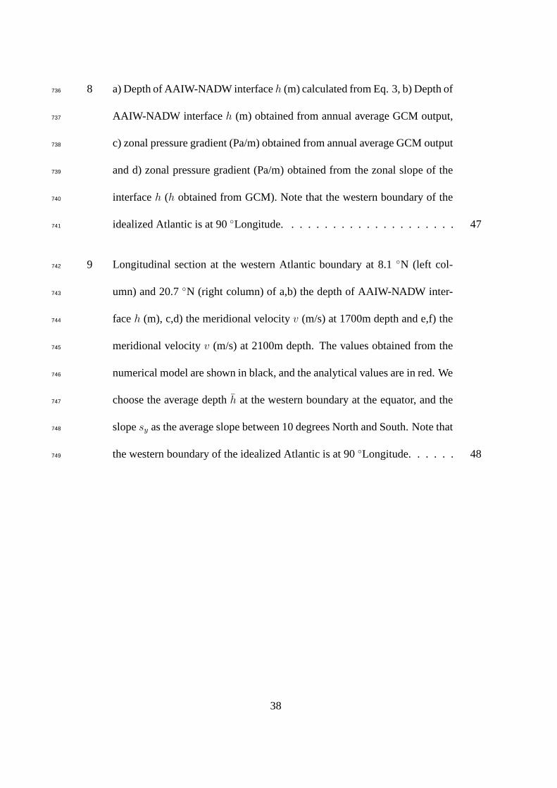
14

To further compare the analytically determinedh and the underlyingv with the GCM, Fig-296

ures 9 and 10 show zonal profiles near the WBC ofh andv at 3 different latitudes and 2297

depths. Again, the analytical solutions do not yieldh, so this value has to be specified. As298

done above,h has been taken as the value ofh at the western boundary at the Equator. We299

checked that similar results to those shown here are obtained for alternative definitions ofh300

, where we choseh inside the ocean interior away from the WB at the latitude of the zonal301

profile (figure not shown), ash is close to its average value also there. Also as above, the302

value ofsy has been determined assy = ∆h∆y

, where the change in quantities∆(y, h) is taken303

between 10◦S and 10◦N in latitude. Again, similar results are obtained for variations of this304

latitudinal domain, provided it remains contained inside the low latitudes. There is a very305

good agreement between the numerical model and the analytical model for the zonal profile306

of h andv at 8.1◦N (Fig. 9 left column) and 8.1◦S (Fig. 10a,b,c), although velocity agrees307

somewhat less at the deeper levelz = −2100m in the southern case (Fig. 10b). Reasonable308

yet reduced agreement is found further away from the Equatorat 20.7◦N (Fig. 9b,d,f), indi-309

cating that the approximation works best near the Equator. The very good agreement of the310

width of the profile near the Equator lends credence to the formulaα = 3

√

( β8AH

) there. The311

overshoot to positive values inv (GCM) away from the western boundary is also present in312

both the numerical model and the analytical solution (e.g. Fig. 9c). The slope∂h∂x

becomes0313

at the western boundary in the analytical solution to allowv = 0 there. This feature is absent314

in the numerical result, as it falls below the model resolution. Nonetheless, the western-most315

v attains a similar value to they-component of the geostrophic velocity in the numerical316

model (see above).317

15

AMOC under varying forcing.318

Figure 11 shows the NADW outflow (at 32◦S), M , for eight other experiments with the319

GCM where we have changed the atmospheric moisture diffusivity (see Section 2) so as to320

achieve different overturning rates in response to alteredbuoyancy fluxes, in order to test321

the general applicability of the analytic description. In each experiment, the model was322

integrated for more than 6000 years in order to attain a steady state. The hydrological cycle323

is meridionally asymmetric in our model, and enhancing moisture diffusivity leads to greater324

freshwater transport to the Southern Ocean (see Saenko and Weaver 2003; Sijp and England325

2008). Increases in the productsy∆ρ (via increasing moisture diffusivity) leads to increased326

NADW outflow M in the numerical model (Fig. 11b), and a generally good agreement is327

maintained between the numerical model andM calculated from Equation (5). In each328

instance the same procedure was followed to obtainsy. We usedD=1200m for the NADW329

outflow depth, instead of the full 1500m, to account for the vertical ramping ofv at the330

water mass boundary. This procedure may need to be more flexible under extreme changes331

in the model asM depends on both∆ρ andsy. Both factors contribute to the increase in332

M (Fig. 11a). Included in the eight experiments are two where the moisture diffusivity field333

has been replaced by a spatially constant field (as in Sijp andEngland 2008). These are334

the two experiments with lowest ratesM (the two left-most points in Fig. 11b), where a335

spatially constant moisture diffusivity of106m2/s leads toM = 7.8Sv and a diffusivity336

of 0.8 × 106m2/s to M = 6.8Sv. Interestingly, the difference inM between these two337

experiments arises almost solely from a difference in slopesy.338

16

Energetics339

The equations of motion yield the time evolution of kinetic energy densityekin via multipli-340

cation byv, giving ∂ekin

∂t= ρ0v

∂v∂t

= ρ0v κ∂2v∂x2−ρ0g

′v ∂h∂y

= ρ0AH∂∂x

(v ∂v∂x

) − ρ0AH(∂v∂x

)2 −341

ρ0g′v ∂h

∂y. The first term of the last expression is a divergence and can be recognised as the342

zonal transport of kinetic energy by viscous forces. The viscous KE transmission is mostly343

zonal and confined inside the western boundary (and so vanishes in the zonal integral), and344

the advection of KE is negligible (as in Gregory and Tailleux2011). The second term,345

−ρ0AH(∂v∂x

)2 = −4ρ0AHv20α

2e−2αxsin2(√

3αx + 23π), is the rate of viscous dissipation of346

energy per unit volume. The third term is the rate of potential energy conversion derived347

from the sloped overlying surfaceh. This term is the rate of work done by the pressure gra-348

dient inside the NADW water column. In steady state∂ekin

∂t= 0, yielding a budget for the349

conversion of potential energy into kinetic energy and theninto heat by viscous dissipation.350

Zonal integration over the WBC domain leaves only the integrals of the viscous dissipation351

rate termρ0AH(∂v∂x

)2 and the potential energy conversion rate−ρ0g′v ∂h

∂y, as the transport352

term vanishes. This means that although the componentv (but not the vector (u,v)) satisfies353

the geostrophic equation, the strong zonal gradient inv near the western boundary allows for354

the conversion of potential energy derived from the meridionally sloped surfaceh into heat355

via viscous dissipation. Locally, the two processes are linked via zonal viscous energy trans-356

port. This situation is shown in Figure 10d, where the energyrate terms are shown. Potential357

energy is converted into kinetic energy near the core of the current, while viscous zonal en-358

ergy transport allows this energy to be dissipated viscously close to the western boundary,359

17

where the gradient inv is the largest. A small amount of this energy is also transported to360

the opposite shoulder away from the western boundary, wherethe gradient inv is also large.361

Gregory and Tailleux (2011) describe the conversion of workdone by the pressure gradient362

into kinetic energy and then heat via viscous dissipation inthe HADCM3 and FAMOUS363

models. Their Figure 4 shows that work done by the pressure gradient is balanced by vis-364

cous dissipation, and that dissipation via horizontal diffusion dominates wherever pressure365

gradient work is positive. This is in agreement with our results. As in Gregory and Tailleux366

(2011), the pressure gradient is allowed to do work as it is not entirely perpendicular to the367

velocity due to vanishingu. In the present analytical model, deviation from geostrophy is368

only due to viscous effects allowingu = 0, a small effect. Gregory and Tailleux (2011) argue369

that even though departure from geostrophy is usually small, it is nevertheless essential for370

the energy budget of the oceans, as it is the term responsiblefor the conversion of potential371

energy into kinetic energy all the way along the western boundary.372

Interestingly, the potential energy is converted from the meridional slope. Although one373

can determinev from the zonal slope∂h∂x

, this tells us little about what physical processes374

determine or limitv. In contrast, the fact that potential energy is converted from the merid-375

ional slope ofh (and due to the∆ρ across it) allows a statement about what global factors376

determinev, namely a portion of the rate of potential energy generationacross the basin.377

Although this is consistent with the view recently advocated by Tailleux (2009) and Hughes378

et al. (2009), it is difficult to infer overturning strength from global energy budgets here. We379

make no attempt to determine this portion from the global energy budgets, and only state380

that once available,sy and∆ρ are such that the rate is proportional to(sy∆ρ)2, and therefore381

18

always positive. Interestingly, the latter quantity is similar to the expression for the available382

potential energy in a two-layer model separated by a horizontally sloping interface, yielding383

a further connection to APE theory. We therefore find that themeridional gradient ofh and384

the density difference across it is a more fundamental determinant ofv than the zonal gradi-385

ent, while the zonal pressure gradient adjusts in response and so yields no information about386

what setsv.387

We can express the zonally integrated energy dissipation rate density (“energy dissipation”388

for short) in terms of the velocity. Recall from Appendix 2 that V (y, z) ≡∫ ∞0

v dx =389

v0

√3

4α(where we takex = 0 at the western basin margin). Then, the energy dissipation is390

W (y, z) ≡∫ ∞0

ρ0AH(∂v∂x

)2 dx = 4ρ0AHα2v20

∫ ∞0

e−2αxsin2(√

3αx + 23π) dx = 3

4ρ0AHαv2

0.391

Here, we have used∫ ∞0

e−2αxsin2(√

3αx + 23π) dx = 3

16α.392

Substitutingv0 and recalling (Appendix 2)α3 = β8AH

, we obtain:393

(6) W = 12ρ0βV 2 = 3

2g2

ρ0β∆ρ2s2

y394

The energy dissipation calculated from model data using (6)is shown in Figure 6c, and395

compares reasonably well with the energy dissipation calculated via the rate of work done396

by the pressure gradient,−∇p · v (Fig. 6b). This lends support to our energy analysis.397

The energy dissipation is confined to the low latitudes whereour approximation works best,398

rendering our framework a good tool for calculating the total energy dissipation associated399

with the lower limb of the AMOC. Equation 6 also suggests thatW ∝ M2. Note thatW400

depends onβ, suggesting that energy dissipation depends on the rotation rate, and its local401

19

rate of change with latitude.402

Undulations inh are associated with available potential energy that could be released by403

pressure work arising from the ensuing pressure gradients.Unlike a non-rotating case, the404

meridional slope ofh near the WB is the only slope from which the available potential energy405

can be released in this manner. This work is done in the lower limb of the AMOC mostly406

at the latitudes where our approximation is most valid, yielding an estimate of the energy407

dissipation rate associated with this flow. The creation of the available potential energy is408

associated with diapycnal mixing, wind stress and surface buoyancy forcing (Hughes et al.409

2009). The precise energy pathways leading to the potentialenergy tied up in the merid-410

ional slope ofh at the WB are diverse and beyond the scope of this study, although we can411

already say that buoyancy forcing changes that increase∆ρ would also increase the work412

done by the meridional pressure gradient field, and so the energy dissipation rate. This is413

then associated with a stronger AMOC. Also, a deeperh would likely yield a largersy, ash414

remains constrained by its outcrop region in the north, leading to a higher energy dissipation415

rate and stronger flow. The available potential energy related toh in the Atlantic is related416

to its average depthh, which in turn is strongly related to the depth ofh at 32◦S, a value417

that is influenced by the SH westerlies. Local wind stress also constrains the shapeh at the418

northern outcrop regions by steepening isopycnals there, suggesting an role for both basin-419

scale wind stress and buoyancy forcing in determiningsy. Also, the steepening ofh near420

its outcrop region suggests that the average depthh determines an upper boundsmaxy to sy,421

namelySmaxy = h/Ly, whereLy is the distance between the equator and the latitude of the422

North Atlantic outcrop region ofh. This also yields an upper bound forM and the potential423

20

energy that can be converted fromh (via pressure work), provided∆ρ remains constant.424

Finally, eddies remove potential energy by flatteningh via the GM parameterisation. This425

effect is strongest in the SO, and less important inside the basin (Kamenkovich and Sarachik426

2004).427

4. Summary and Conclusions428

We have proposed a new analytical description of the AAIW-NADW interfaceh and the429

underlying DWBC at low latitudes. This has allowed us to understand the processes limiting430

the NADW outflow rate, and the mechanisms that make the flow locally dependent on the431

AAIW-NADW density difference. Our approach works best nearthe Equator (e.g. between432

10◦S and 10◦N), and becomes somewhat less accurate at high northern latitudes and around433

30 ◦S. Nonetheless, the low latitude validity of the description allows us to obtain a more434

general scaling for the NADW outflow rateM , as the flow must pass the low latitudes to exit435

the basin. Our approximation to the vertical profile ofv is a Heaviside function, whereas the436

GCM exhibits a more gradual profile sculpted by further subtle density transitions inside the437

NADW column. Despite the simplicity of this approximation,a function forM in terms of438

sy∆ρ is obtained that compares very favourably to the GCM. We offer no precise description439

of how buoyancy forcing affects the density field, although this will be needed in a future440

study to link the overturning to surface forcing. Finally, our approach does not capture the441

underlying AABW cell and does not yield an expression for theNADW column thickness442

D. Instead, this must be estimated from the GCM output. Furthermore, no description is443

21

offered of the upper branch of the AMOC.444

A brief energy analysis shows that potential energy arisingfrom the meridional slope ofh is445

converted into kinetic energy and then viscously dissipated. This yields a constraint on the446

flow, namely the rate of basin-wide potential energy production via this slope. In contrast,447

the zonal slope is a passive response arising from a geostrophic adjustment mechanism,448

perhaps similar in essence to that described in Johnson and Marshall (2002). Indeed, the449

deep meridional velocity can be derived from the zonal pressure gradient via a thermal wind450

balance, but this procedure yields no information about thedriving mechanisms maintaining451

this dissipative flow. Gregory and Tailleux (2011) also emphasise the role of this energy452

conversion process in limiting the NADW overturning rate. The analytical expression forh453

(Eq. 3) provides a relationship between the zonal and meridional pressure gradient.454

Scaling of the upper limb of the AMOC generally involves linking zonal to meridional pres-455

sure gradients and velocities, and employ basin-wide zonalscales (see De Boer et al. 2010,456

for a discussion). In contrast, we show here that the zonal scales of these quantities are the457

WBC width for the AMOC lower limb. Here, the AMOC is describedas a dissipative system458

largely confined to the western boundary region, where available potential energy associated459

with local density structure is converted into kinetic energy, yielding a constant velocity sub-460

ject to viscous drag at each latitude. This suggests the importance of future investigation461

of the relationship between this study and the studies by Hughes et al. (2009) and Tailleux462

(2009), who stress the importance of available potential energy in facilitating the transfer of463

kinetic energy to the background potential energy in maintaining the AMOC, and that the464

22

rate of transfer between different energy reservoirs is more important than the total available465

potential energy.466

Our deep circulation differs from that proposed by Stommel and Arons (1960), who assume467

a uniform abyssal upwelling across the Atlantic thermocline base. In contrast, we assume468

little or no low-latitude Atlantic upwelling, as in observations (Talley et al. 2003) and our469

numerical model (see Section 2). Also, the horizontal abyssal recirculation characteristic of470

the Stommel and Arons (1960) model is absent in our numericalmodel (Fig. 2) and analytical471

model. The Stommel and Arons (1960) approach regards the DWBC as a passive response472

to the introduction of a mass source (deep sinking) in the deep layer located in the North473

Atlantic. In contrast, in our approach the DWBC is coupled tothe overlying interfacial474

surfaceh, and both interact to evolve to a steady state.475

Our experiments take place in a flat bottom idealised numerical model below eddy permitting476

resolution, yielding a relatively quiescent deep circulation away from the western boundary.477

In contrast, several recent observational studies find thatsubsurface floats injected within478

the DWBC of the Labrador Sea are commonly advected into the North Atlantic deep in-479

terior, in apparent contrast to the view that the deep water formed in the North Atlantic480

predominantly follows the DWBC (e.g. Bower et al. 2009; Lozier 2010). Indeed, in the481

ocean eddy-permitting model of Spence et al. (2011), a portion of NADW separates from the482

western boundary and enters the low-latitude Atlantic via interior pathways distinct from the483

DWBC, with a the total southward transport off shore of the DWBC of about 5Sv at 35◦N.484

However, unlike the model used in the present study, that study employs also a detailed ocean485

23

bathymetry while the present study seeks to isolate the AMOCscaling factors in a simple486

setting. Furthermore, the NADW recirculation described inSpence et al. (2011) takes place487

at or to the north of our domain of interest while, as in our study, southward flow is the norm488

within most of the low latitudes also in their model. Also, our approach assumes a dominant489

role for the viscous dissipation of momentum in the horizontal direction, whereas in the real490

system bottom pressure torques may play a significant role (Hughes and de Cuevas 2001).491

However, the results discussed here apply to non-eddy resolving models, and provide a better492

understanding of their behaviour. Furthermore, the details of the energy dissipation can be493

adjusted in our framework.494

De Boer et al. (2010) find that the AMOC scale depth is set by thedepth of the maximal495

AMOC streamfunction, instead of the pycnocline depth, and emphasise that these depths496

differ. This is in agreement with our experiments, ash represents this scale depth. However,497

although the meridional slopesy of h at the western boundary is related toh becauseh must498

outcrop near the northern boundary, we find no direct or simple way to linksy to h. This499

is because the slope∂h∂y

is only constant along the boundary at low latitudes, and increases500

sharply north of 50◦N. There is an indirect link, as deepening ofh would yield greater501

isopycnal slopes near the northern boundary, and thereforemore available potential energy.502

The availability of this extra potential energy to the AMOC then determines howsy increases503

with h. Processes influencingh take place in the Southern Ocean (e.g. Gnanadesikan 1999)504

as well as via diapycnal mixing and the horizontal distribution of buoyancy at the ocean505

surface, thus supplying energy to the deep WBC and determining outflow rates. Furthermore,506

AABW constrains the vertical extentD of the AMOC lower limb as well as influencingh,507

24

providing a further constraint.508

We determine the constants needed in ourM scaling more directly from our numerical model509

so that we can verify our formula against numerical model results without tuning the result510

to fit the overturning rate or deep velocities, yielding a good validation of our analytical511

model. Nonetheless, our basin-geometry is rectangular, and our approach may require the512

introduction of further geometrical factors in models witha more realistic and irregular ge-513

ometry. Furthermore, geometrical factors enter our considerations via the choice of location514

where we conduct our analysis (low latitudes) and the depth-rangeD of the NADW outflow.515

Nonetheless, we provide further insight into the origins ofgeometrical constants and pro-516

vide a scaling where factors can be obtained from GCM output (Eq. 6). We link this to the517

local mechanisms at play in driving the NADW outflow. The depth of the NADW outflow,518

the density difference between the stacked water masses andthe meridional slope of their519

interface at the western boundary need to be determined to yield the NADW outflow rate.520

Appendix 1. Vanishing pressure gradient on interfaceh521

We examine an isopycnal surfaceh of densityρh situated between the tongues of AAIW522

and NADW moving in opposite directions. These flows are essentially pressure-driven (see523

also Gnanadesikan 1999), andh resides inside a depth range where velocities and pressure524

gradients are small (see Fig. 7b). We assume the ocean is in hydrostatic balance i.e.∂p∂z

=525

−gρ for z increasing in the upward direction and zero at the sea surface, wherep is pressure,526

25

g gravity andρ ocean density. Therefore,∂∇Hp∂z

= −g∇Hρ, yielding∇Hp(z) = ∇Hp0 +527

g∫ 0

z∇Hρ(z) dz, where∇Hp0 is the rigid lid pressure gradient at the lid surfacez = 0. The528

gradient∇H denotes the horizontal gradient( ∂∂x

, ∂∂y

, 0). We will only be concerned with529

horizontal pressure gradients and velocities, as isopycnal slopes are very small in our region530

of interest, and the horizontal velocity scale generally exceeds the vertical velocity scale by531

a factor of104. The interface depthh is simply such that∇Hp = 0 atz = h (Assumption 1),532

so for anyz < h, ∇Hp(z) = ∇Hp0 + g∫ 0

h∇Hρ(z) dz + g

∫ h

z∇Hρ(z) dz = g

∫ h

z∇Hρ(z) dz.533

Hence the geostrophic velocityv(z) = 1/fρ0 ∂p/∂x = g/fρ0

∫ h

z∂ρ/∂x dz, and similarly534

for u(z).535

Now, along an isopycnal surfacezρ of densityρ, we have: ∂ρ∂x

dx + ∂ρ∂y

dy + ∂ρ∂z

dz = 0, so536

∂ρ∂x

= −∂ρ∂z

∂zρ

∂x, wherezρ denotes the depth of the isopycnal of densityρ. Then537

v(z) = − gρ0f

∫ h

z∂ρ(z)

∂z∂zρ

∂xdz538

We now approximate the density distribution overz ∈ [−∞, h] as ρ(z) = ρNADW −539

(ρNADW − ρAAIW )H(z − h), whereH is the Heaviside function. Note that we gener-540

ally takeρNADW to be the density at the western boundary, the Equator and 1800m depth541

(the core of the outflow).ρAAIW is defined at the same horizontal location at 1000m depth.542

This crude approximation to the density field amounts to assigning a single uniform density543

to the NADW water massρNADW , and assuming a relatively rapid density transition from544

ρAAIW to ρNADW acrossh (Assumption 3). Then,∂ρ∂z

= −(ρNADW − ρAAIW )δ(z − h),545

whereδ is the Dirac delta function, and substituting this in the z-integral givesv(z) =546

gρ0f

(ρNADW − ρAAIW )∂h∂x

= g′

f∂h∂x

for z < h, whereg′ = g∆ρρ0

is the reduced gravity. We547

26

generally assume the beta plane approximationf ≈ βy. We estimate an effective thick-548

nessD of about 1200m for the NADW outflow, leading to a maximal NADW outflow depth549

h+1200 ≈ 2400m. This choice can be regarded as a “geometrical factor” (see Introduction),550

and visual inspection of Fig. 1 suggests it is a reasonable choice. We ignore the contribution551

to the NADW outflow below this depth, as by definition the NADW flow resides above the552

zero contour (Fig. 1). We definev = 0 there for our purposes. In reality, further density553

gradients give rise to a reduction in flow below the NADW. The zonal maxima of the analyt-554

ically determined meridional velocity generally coincidewith v at the western-most Atlantic555

grid cell in the GCM (Fig. 9 and Fig. 10).556

Appendix 2. Derivation of solution to equations of motion.557

Here we derive useful solutions to the equations of motion Eqs. 1,2. We restate the equations558

in the more general form usingf , and without the beta plane approximation used in the main559

text (the approximation will be introduced below):560

(1’) 0 = ∂u∂t

= fv − g′ ∂h∂x

561

(2’) 0 = ∂v∂t

= AH∂2v∂x2 − fu − g′ ∂h

∂y562

Recall thatu ≈ 0, which will be used below. We cross differentiate the equations of motion563

to obtain the vorticity equation−AH∂3v∂3x

+ βv + f(∂u∂x

+ ∂v∂y

) = 0. Near the equator, where564

f goes to zero, the vorticity balance is well approximated by∂3v∂3x

= βvAH

. Note also that the565

27

weak NADW recirculation in our model (Fig. 1, Assumption 4) renders the horizontal flow566

largely divergence-free inside the NADW depth range, also rendering the 3rd term small.567

Interestingly, this equation can be recognised as that governing the boundary-layer solution568

in Munk (1950)’s model of wind-driven circulation. The physically acceptable solution along569

the western boundary is simply given byv = v0(y)e−αxsin(√

3αx) g′

β, wherev0(y) is an570

undetermined function ofy, andα = r1/2 = 12( β

AH)1/3. Note thatv appears separable in571

x andy. This motivates writingh = h + F (x)G(y). F represents a longitudinal profile572

while G is the latitudinal amplification of this profile to satisfy geostrophy in Eq. (1’), where573

G(0) = 0. As we are only discussing the dynamics for the low latitudes, we shall now574

assume aβ-plane approximation, and take forβ its value at the Equator. Equations (1)575

and (2) indicates a close correspondence between thex-dependence ofv andh, and trying576

h(x, y) =h +y sye−αx(

√3

3sin(

√3αx) + cos(

√3αx)) givesv0 = − g′sy

2√

3AHα2= − 4√

3syα

g′

β577

wheresy is simply the constant slope ofh at the western boundary. It is likely determined by578

non-local factors. Also,u = 0 (−βyu is the only y-dependent term in Eq. 2). The integrated579

transport in the boundary layer is therefore580

V = v0(y)∫ ∞0

e−αxsin(√

3αx) dx = v0(y)√

34α

= −g′sy

√3

β581

which is independent ofAH , as in Munk (1950). Note that here we takex = 0 at the western582

basin margin.583

Multiplying V by the vertical extent of the NADW columnD yields the NADW outflow. We584

thus assume that the variations inh are small compared toD. This yields Equations 3, 4 and585

5.586

28

Acknowledgements. We thank the University of Victoria staff for support in usage of their587

coupled climate model. This research was supported by the Australian Research Council588

and the Australian Antarctic Science Program. This research was undertaken on the NCI589

National Facility in Canberra, Australia, which is supported by the Australian Common-590

wealth Government. We thank Andreas Oschlies for hosting a visit to IFM-GEOMAR and591

supplying code and advice to allow W. P. Sijp to implement theturbulent kinetic energy592

scheme of Blanke and Delecluse (1993) based on Gaspar et al. (1990) into the model.593

29

References594

Blanke, B. and P. Delecluse, 1993: Variability of the tropical Atlantic ocean simulated by a595

general circulation model with two different mixed-layer physics.J. Phys. Oceanogr., 23,596

13631388.597

Bower, A., M. Lozier, S. Gary, and C. Boning, 2009: Interior pathways of the North Atlantic598

meridional overturning circulation.Nature, 459, 243–248.599

Bryan, F., 1987: Parameter sensitivity of primitive equation ocean general circulation mod-600

els.Journal of Physical Oceanography, 17, 970–985.601

De Boer, A. M., A. Gnanadesikan, N. R. Edwards, and A. J. Watson, 2010: Meridional602

density gradients do not control the Atlantic overturning circulation.Journal of Physical603

Oceanography, 40, 368–380.604

Dijkstra, H. A., 2008: Scaling of the Atlantic meridional overturning in a global ocean605

model.Tellus, 60a, 749–760.606

Gaspar, P., Y. Gregoris, and J. M. Lefevre, 1990: A simple eddy kinetic energy model for607

simulations of the oceanic vertical mixing: Tests at station papa and long-term upper ocean608

study site.J. Geophys. Res., 95, 1617916193.609

Gent, P. R. and J. C. McWilliams, 1990: Isopycnal mixing in ocean general circulation610

models.Journal of Physical Oceanography, 20, 150–155.611

Gerdes, R., C. Koberle, and J. Willebrand, 1991: The influence of numerical advection612

30

schemes on the results of ocean general circulation models.Climate Dynamics, 5, 211–613

226.614

Gnanadesikan, A., 1999: A simple predictive model for the structure of the oceanic pycno-615

cline.Science, 283, 2077–2079.616

Gnanadesikan, A., A. M. de Boer, and B. K. Mignone, 2007: A simple theory of the pycno-617

cline and overturning revisited.Geophysical Monograph American, 173, 19–32.618

Gregory, J. M. and R. Tailleux, 2011: Kinetic energy analysis of the response of the Atlantic619

meridional overturning to CO2-forced climate change.Climate Dynamics (In Press), -,620

DOI 10.1007/s00382–010–847–6.621

Griesel, A. and M. A. Morales-Maqueda, 2006: The relation ofmeridional pressure gradients622

to North Atlantic deep water volume transport in an ocean general circulation model.623

Climate Dynamics, 26, 781–799.624

Hughes, C. and B. de Cuevas, 2001: Why western boundary currents in realistic oceans625

are inviscid: a link between form stress and bottom pressuretorques.Journal of Physical626

Oceanography, 31, 2871–2885.627

Hughes, G. O., A. M. C. Hogg, and R. W. Griffiths, 2009: Available potential energy and ir-628

reversible mixing in the meridional overturning circulation.Journal of Physical Oceanog-629

raphy, 39, 3130–3146.630

Hughes, T. M. C. and A. J. Weaver, 1994: Multiple equilibria of an asymmetric two-basin631

ocean model.Journal of Physical Oceanography, 24, 619–637.632

31

Johnson, H. and D. P. Marshall, 2002: A theory for the surfaceAtlantic response to thermo-633

haline variability.Journal of Physical Oceanography, 32, 1121–1132.634

Kalnay, E., M. Kanamitsu, R. Kistler, W. Collins, D. Deaven,L. Gandin, M. Iredell, S. Saha,635

G. White, J. Woollen, Y. Zhu, A. Leetmaa, and R. Reynolds., 1996: The NCEP/NCAR636

40-year re-analysis project.Bull. Amer. Meteor. Soc., 77, 437–471.637

Kamenkovich, I. V. and P. J. Goodman, 2000: The dependence ofAABW transport in the638

Atlantic on vertical diffusivity.Geophysical Research Letters, 27, 3739–3742.639

Kamenkovich, I. V. and E. S. Sarachik, 2004: Mecahnisms controlling the sensitivity of640

the Atlantic ThermohalineCirculation to the parameterization of eddy transports in ocean641

GCM. Journal of Physical Oceanography, 34, 1628–1647.642

Levermann, A. and J. J. Fuerst, 2010: Atlantic pycnocline theory scrutinized using a coupled643

climate model.Geophysical Research Letters, 37, doi:10.1029/2010GL044180.644

Levermann, A. and A. Griesel, 2004: Solution of a model for the oceanic pycnocline depth:645

Scaling of overturning strength and meridional pressure difference.Geophysical Research646

Letters, 31, doi:10.1029/2004GL020678.647

Lozier, M., 2010: Deconstructing the conveyor belt.Science, 328, 1507–1511.648

Manabe, S. and R. J. Stouffer, 1988: Two stable equilibria ofa coupled ocean-atmosphere649

model.Journal of Climate, 1, 841–866.650

— 1999: Are two modes of thermohaline circulation stable?Tellus, 51A, 400–411.651

32

Marotzke, J., 1997: Boundary mixing and the dynamics of three-dimensional thermohaline652

circulations.Journal of Physical Oceanography, 27, 1713–1728.653

Munk, W. H., 1950: on the wind-driven ocean circulation.Journal of Meteorology, 7, 3–29.654

Pacanowski, R., 1995:MOM2 Documentation User’s Guide and Reference Manual: GFDL655

Ocean Group Technical Report 3. NOAA, GFDL. Princeton, 3 edition, 232pp.656

Park, Y. G. and J. A. Whitehead, 1999: Rotating convection driven by differential bottom657

heating.Journal of Physical Oceanography, 29, 1208–1220.658

Rahmstorf, S., 1996: On the freshwater forcing and transport of the Atlantic thermohaline659

circultion.Climate Dynamics, 12, 799–811.660

Robinson, A. R., 1960: The general thermal circulation in equatorial regions.Deep-Sea661

Research, 6, 311–317.662

Robinson, A. R. and H. Stommel, 1959: The oceanic thermocline and the associated ther-663

mohaline circulation.Tellus, 11, 295–308.664

Saenko, O. A. and A. J. Weaver, 2003: Atlantic deep circulation controlled by freshening in665

the Southern Ocean.Geophysical Research Letters, 30, doi:10.1029/2003GL017681.666

Schewe, J. and A. Levermann, 2010: The role of meridional density differences for a wind-667

driven overturning circulation.Climate Dynamics, 34, 547–556.668

Sijp, W. P. and M. H. England, 2004: Effect of the Drake Passage throughflow on global669

climate.Journal of Physical Oceanography, 34, 1254–1266.670

33

— 2008: Atmospheric moisture transport determines climaticresponse to the opening of671

drake passage.Journal of Climate (submitted), 0, 0.672

Spence, P., O. Saenko, W. P. Sijp, and M. England, 2011: The role of bottom pressure torque673

on the interior pathways of NADW.Journal of Physical Oceanography (accepted), –, –.674

Stommel, H. and A. B. Arons, 1960: On the abyssal circulationof the world ocean, I. an675

idealized model of the circulation pattern and amplitude inoceanic basins.Deep-Sea Res.,676

6, 217–233.677

Tailleux, R., 2009: On the energetics of stratified turbulent mixing, irreversible thermo-678

dynamics, boussinesq models, and the ocean heat engine controversy.Journal of Fluid679

Mechanics, 639, 339–382.680

Talley, L. D., J. L. Reid, and P. E. Robbins, 2003: Data-basedmeridional overturning stream-681

functions for the global ocean.Journal of Climate, 16, 3213–3226.682

Thorpe, R. B., J. M. Gregory, T. C. Johns, R. A. Wood, and J. F. B. Mitchell, 2001: Mecha-683

nisms determining the Atlantic thermohaline circulation response to greenhouse gas forc-684

ing in a non-flux-adjusted coupled climate model.Journal of Climate, 14, 3102–3116.685

Vellinga, M. and R. A. Wood, 2002: Global climatic impacts ofa collapse of the Atlantic686

thermohaline circulation.Climate Change, 54, 251–267.687

Warren, B. A., 1976: Structure of deep western boundary currents.Deep-Sea Research, 23,688

129–142.689

34

Weaver, A. J., M. Eby, E. C. Wiebe, and co authors, 2001: The UVic Earth System Cli-690

mate Model: model description, climatology, and applications to past, present and future691

climates.Atmosphere-Ocean, 39, 1067–1109.692

Wright, D. G. and T. F. Stocker, 1991: zonally averaged oceanmodel for thermohaline circu-693

lation. part i. model development and flow dynamics.Journal of Physical Oceanography,694

21, 1713–1724.695

Wright, D. G., C. B. Vreugdenhil, and T. M. C. Hughes, 1995: Vorticity dynamics and696

zonally averaged ocean circulation models.Journal of Physical Oceanography, 25, 2141–697

2154.698

35

List of Figures699

1 Atlantic meridional overturning streamfunction, 10 yearaverage. Obtained700

via vertical integration of the basin-wide zonal integral of v. Positive values701

indicate clockwise flow. Values are given in Sv (1 Sv = 106 m3 sec−1). . . . 40702

2 Direction of NADW flow at 2160m depth in the Atlantic. A typical velocity703

in the WBC is 3 cm/s. Taken from 10 year average. . . . . . . . . . . . .. 41704

3 Depth of isopycnalh that lies between the AAIW and NADW tongues in705

the Atlantic (depth in m). The narrow basin displayed near the centre of the706

figure is identified with the Atlantic basin. We generally take x = 0 at the707

western boundary of this basin. Taken from 10 year average. .. . . . . . . 42708

4 Schematic representation of AMOC lower limb and the AAIW-NADW in-709

terface h. The interface h assumes its average depth and has avery small lat-710

itudinal (y) slope in the interior away from the western boundary (dashed),711

and has a constantant positive latitudinal slope at the boundary (solid), where712

it attains its average value only at the equator (where the solid and dashed713

lines intersect). The vertical displacement of h from its average depth at the714

western boundary leads to a zonal pressure gradient and a meridional flow v,715

where the direction into the page is indicated by a cross inside a circle (x, on716

the right) and out of the page by a very small + inside a circle (on the left). 43717

36

5 Values at the Atlantic western boundary grid cell of a) the meridional veloc-718

ity v (m/s) at 8.1◦N where values from the numerical model are black and719

values from the analytical theory are red, b)σ (kg/m3) with ρ referenced to720

1200m depth and c) an idealization of the density at the western boundary.721

The interfaceh is indicated by a bold contour in (b). The idealization in722

(c) approximatesσ in the NADW depth range byσNADW andσ aboveh by723

σAAIW . Taken from 10 year average. . . . . . . . . . . . . . . . . . . . . . 44724

6 a) Atlantic western boundary grid cell values of geostrophic meridional ve-725

locity vgeos divided by the actual meridional velocityv in the model,vgeos

v.726

b) The zonal total of the energy dissipation rate density (W/m2) calculated727

over the western boundary layer via work done by the pressuregradient, and728

calculated as the zonal integral of∇p · v. c) Same as (b), but calculated via729

12ρ0βV 2, whereV =

∫ ∞0

v(x) dx. Note that we omit equatorial values of730

vgeos/v in (a), asf vanishes there. . . . . . . . . . . . . . . . . . . . . . . 45731

7 Values at western Atlantic boundary of a) meridional velocity v (m/s) and b)732

zonal pressure gradient (Pa/m). Overlaid are the depth of the AAIW-NADW733

interfacial isopycnal at the western boundary (solid) and 5◦longitude east of734

the western boundary (dashed). . . . . . . . . . . . . . . . . . . . . . . . .46735

37

8 a) Depth of AAIW-NADW interfaceh (m) calculated from Eq. 3, b) Depth of736

AAIW-NADW interface h (m) obtained from annual average GCM output,737

c) zonal pressure gradient (Pa/m) obtained from annual average GCM output738

and d) zonal pressure gradient (Pa/m) obtained from the zonal slope of the739

interfaceh (h obtained from GCM). Note that the western boundary of the740

idealized Atlantic is at 90◦Longitude. . . . . . . . . . . . . . . . . . . . . 47741

9 Longitudinal section at the western Atlantic boundary at 8.1 ◦N (left col-742

umn) and 20.7◦N (right column) of a,b) the depth of AAIW-NADW inter-743

faceh (m), c,d) the meridional velocityv (m/s) at 1700m depth and e,f) the744

meridional velocityv (m/s) at 2100m depth. The values obtained from the745

numerical model are shown in black, and the analytical values are in red. We746

choose the average depthh at the western boundary at the equator, and the747

slopesy as the average slope between 10 degrees North and South. Notethat748

the western boundary of the idealized Atlantic is at 90◦Longitude. . . . . . 48749

38

10 Longitudinal section at the western Atlantic boundary at8.1 ◦S (not to be750

confused with previous Figure showing 8.1◦N) of a) the depth of AAIW-751

NADW interfaceh (m), b) the meridional velocityv (m/s) at 2100m depth,752

c) the meridional velocityv (m/s) at 1700m depth and d) the rate of energy753

conversion terms (10−6W/m3): potential energy (blue), viscous dissipation754

(black) and viscous transfer (red). The values obtained from the numerical755

model in (a), (b) and (c) are shown in black, and the analytical values are in756

red. h andsy are chosen as in the previous figure. . . . . . . . . . . . . . . 49757

11 Experiments where atmospheric moisture diffusivity is varied to accomplish758

oceanic surface buoyancy flux changes. a) NADW outflow rateM (Sv) as a759

function of the meridional slopesy = ∂h∂y

of h and the AAIW-NADW density760

difference∆ρ (kg/m3). Numerical experiment values are marked by a *. b)761

NADW outflow rateM (Sv) vs. the productsy∆ρ (kg/m3) for the numerical762

model (red) and analytical model (black). . . . . . . . . . . . . . . .. . . 50763

39

−20 0 20 40 60 80−5500

−5000

−4500

−4000

−3500

−3000

−2500

−2000

−1500

−1000

−500

0

LATITUDE

DE

PT

H (

m)

−9−8 −7−6−5−4−3

−3

−3

−2

−2

−2

−1

−1

−1

0 0

0

0

0

2

2 2

24

4

4

46

6

6

66

8

8

88

10

10

10

12

12

12

14

14

1618

Atlantic Meridional Stream Function (Sv)

Figure 1: Atlantic meridional overturning streamfunction, 10 year average. Obtained via

vertical integration of the basin-wide zonal integral ofv. Positive values indicate clockwise

flow. Values are given in Sv (1 Sv = 106 m3 sec−1).

40

100oE 120

oE 140oE 160oE 180oW

20oS

0o

20oN

40oN

60oN

80oN

Velocity at 2160m depth

LONGITUDE

LAT

ITU

DE

Figure 2: Direction of NADW flow at 2160m depth in the Atlantic. A typical velocity in the

WBC is 3 cm/s. Taken from 10 year average.

41

50 100 150 200 250 300 350

−80

−60

−40

−20

0

20

40

60

80

LONGITUDE

LAT

ITU

DE

200100

1600160015001400

1300

1300

18002300

1200

1400 15001500

1500

15001500

1500

15001600

15001100700400400

500 600300200100100100

8001200

1500

Depth of AAIW−NADW interface h

0

200

400

600

800

1000

1200

1400

1600

1800

2000

Figure 3: Depth of isopycnalh that lies between the AAIW and NADW tongues in the

Atlantic (depth in m). The narrow basin displayed near the centre of the figure is identified

with the Atlantic basin. We generally takex = 0 at the western boundary of this basin.

Taken from 10 year average.

42

Figure 4: Schematic representation of AMOC lower limb and the AAIW-NADW interface

h. The interface h assumes its average depth and has a very small latitudinal (y) slope in the

interior away from the western boundary (dashed), and has a constantant positive latitudinal

slope at the boundary (solid), where it attains its average value only at the equator (where

the solid and dashed lines intersect). The vertical displacement of h from its average depth at

the western boundary leads to a zonal pressure gradient and ameridional flow v, where the

direction into the page is indicated by a cross inside a circle (x, on the right) and out of the

page by a very small + inside a circle (on the left).

43

Figure 5: Values at the Atlantic western boundary grid cell of a) the meridional velocityv

(m/s) at 8.1◦N where values from the numerical model are black and values from the ana-

lytical theory are red, b)σ (kg/m3) with ρ referenced to 1200m depth and c) an idealization

of the density at the western boundary. The interfaceh is indicated by a bold contour in (b).

The idealization in (c) approximatesσ in the NADW depth range byσNADW andσ aboveh

by σAAIW . Taken from 10 year average.

44

−2800

−2600

−2400

−2200

−2000

−1800

−1600

−1400

−1200

0.8

0.80.85 0.85

0.9

0.9

0.95

0.95

1 1

1

1

DE

PT

H

(a) Quotient geostr. v/ v at west. boundary

−2800

−2600

−2400

−2200

−2000

−1800

−1600

−1400

−1200 0.2

0.2

0.4

0.4 0.4

0.4

0.6

0.6

0.6

0.8

0.8

0.8

1

1

DE

PT

H

(b) Rate of work done by ∇ P (W/m3) at west. boundary

−20 −10 0 10 20 30 40

−2800

−2600

−2400

−2200

−2000

−1800

−1600

−1400

−1200 0.2

0.2

0.40.4

0.4

0.4 0.6

0.6

0.6

0.8

0.8

0.8

1

1

1.2

1.2

1.4

DE

PT

H

LATITUDE

(c) Energy dissipation rate (W/m3) calculated as 1/2ρ0β V2

Figure 6: a) Atlantic western boundary grid cell values of geostrophic meridional velocity

vgeos divided by the actual meridional velocityv in the model,vgeos

v. b) The zonal total of the

energy dissipation rate density (W/m2) calculated over the western boundary layer via work

done by the pressure gradient, and calculated as the zonal integral of∇p · v. c) Same as (b),

but calculated via12ρ0βV 2, whereV =

∫ ∞0

v(x) dx. Note that we omit equatorial values of

vgeos/v in (a), asf vanishes there.

45

Figure 7: Values at western Atlantic boundary of a) meridional velocityv (m/s) and b) zonal

pressure gradient (Pa/m). Overlaid are the depth of the AAIW-NADW interfacial isopycnal

at the western boundary (solid) and 5◦longitude east of the western boundary (dashed).

46

Figure 8: a) Depth of AAIW-NADW interfaceh (m) calculated from Eq. 3, b) Depth of

AAIW-NADW interfaceh (m) obtained from annual average GCM output, c) zonal pressure

gradient (Pa/m) obtained from annual average GCM output andd) zonal pressure gradient

(Pa/m) obtained from the zonal slope of the interfaceh (h obtained from GCM). Note that

the western boundary of the idealized Atlantic is at 90◦Longitude.

47

−1230

−1190

−1150

−1110

−1070

−1030

m

(a) AAIW−NADW interface depth h at 8.1 ° N

−1230

−1190

−1150

−1110

−1070

−1030

m

(b) AAIW−NADW interface depth h at 20.7 ° N

−0.04

−0.03

−0.02

−0.01

0

0.01

m/s

(c) meridional velocity v at z=1700m at 8.1 ° N

GCMAnalytical

−0.04

−0.03

−0.02

−0.01

0

0.01

m/s

(d) meridional velocity v at z=1700m at 20.7 ° N

GCMAnalytical

90 100 110 120 130−0.04

−0.03

−0.02

−0.01

0

0.01

m/s

LONGITUDE

(e) meridional velocity v at z=2100m at 8.1 ° N

GCMAnalytical

90 100 110 120 130−0.04

−0.03

−0.02

−0.01

0

0.01

m/s

LONGITUDE

(f) meridional velocity v at z=2100m at 20.7 ° N

GCMAnalytical

Figure 9: Longitudinal section at the western Atlantic boundary at 8.1◦N (left column)

and 20.7◦N (right column) of a,b) the depth of AAIW-NADW interfaceh (m), c,d) the

meridional velocityv (m/s) at 1700m depth and e,f) the meridional velocityv (m/s) at 2100m

depth. The values obtained from the numerical model are shown in black, and the analytical

values are in red. We choose the average depthh at the western boundary at the equator, and

the slopesy as the average slope between 10 degrees North and South. Notethat the western

boundary of the idealized Atlantic is at 90◦Longitude.

48

−1280

−1250

−1220

−1190

m

(a) AAIW−NADW interface depth h

−0.04

−0.03

−0.02

−0.01

0

0.01

m/s

(b) meridional velocity v at 2100m depth

GCMAnalytical

90 100 110 120 130−0.04

−0.03

−0.02

−0.01

0

0.01

m/s

LONGITUDE

(c) meridional velocity v at 1700m depth

GCMAnalytical

90 100 110 120 130 140−6

−3

0

3

6

9

12

15

10−

6 W/m

3

LONGITUDE

(d) Energy terms rate of change.

Pot. En.Visc. Diss.Visc. Transf.

Figure 10: Longitudinal section at the western Atlantic boundary at 8.1◦S (not to be con-

fused with previous Figure showing 8.1◦N) of a) the depth of AAIW-NADW interfaceh

(m), b) the meridional velocityv (m/s) at 2100m depth, c) the meridional velocityv (m/s)

at 1700m depth and d) the rate of energy conversion terms (10−6W/m3): potential energy

(blue), viscous dissipation (black) and viscous transfer (red). The values obtained from the

numerical model in (a), (b) and (c) are shown in black, and theanalytical values are in red.

h andsy are chosen as in the previous figure.

49

2.6 2.8 3 3.2 3.4 3.6 3.8 4 4.2 4.4

x 10−5

0.25

0.3

0.35

0.4

67

88

9

9

10

10

11

11

12

12

13

14

15

∆ρy (

kg/m

3 )

Slope sy = dh/dy

(a) ∆ρy vs. y−slope h with NADW outflow contours

0.6 0.8 1 1.2 1.4 1.6 1.8 2

x 10−5

0

2

4

6

8

10

12

14

16

18

sy∆ρ

y (kg/m3)

NA

DW

out

fl (S

v)

(b) NADW outflow vs product s

y∆ρ

y

AnalyticalGCM

Figure 11: Experiments where atmospheric moisture diffusivity is varied to accomplish

oceanic surface buoyancy flux changes. a) NADW outflow rateM (Sv) as a function of

the meridional slopesy = ∂h∂y

of h and the AAIW-NADW density difference∆ρ (kg/m3).

Numerical experiment values are marked by a *. b) NADW outflowrateM (Sv) vs. the

productsy∆ρ (kg/m3) for the numerical model (red) and analytical model (black).

50