.

The information loss during black holeevaporation: A novel approach to diffusing

the ”paradox”

Daniel Sudarsky, ICN-UNAM.Collaboration with: E. Okon, S. Modak, L. Ortız, & I. Pena“Benefits of Objective Collapse Models for Cosmology and

Quantum Gravity” Found. of Phys. 44, 114 (2014);“The Black Hole Information Paradox and the Collapse of

the Wave Function” Found. of Phys. 45, 461 (2015).“ Non-Paradoxical Loss of Information in Black Hole

Evaporation in Collapse Theories” Phys. Rev. D 91, 124009(2015);

“Black Holes: Information Loss But No Paradox ” Gen. Rel.& Gravitation 47 , 120 (2015); arXiv:1406.4898 [gr-qc]

January 29, 2016

End point of massive star’s evolution .. stationary are blackholes (BH) . Characterized M,Q,&J.

Formation of (BH), ...large amount of information loss.

Refers only to that available to the exterior observers .

The complete space-time, and matter fields can be recoveredusing data located both outside and inside the black holeregion. Nothing is really puzzling.

QT changes things: S. Hawking QFT effects cause BH toradiate. It should loose mass & eventually disappear ( unless...).

Distant observers ”see” the BH mass going to 0 in a finite time.After the evaporation is completed, we would have justMinkowski space-time.

What about the loss of information issue now?People’s postures depend on what they assume about thesingularity, and their ideas regarding what physical theoriesshould be about.

A possible way out : consider the singularity (or, more precisely,a region arbitrarily close to it) as the boundary of space-time.Then, one might argue that information “ends up” at, or,“escapes through” the singularity.

Not satisfactory for workers on QG. They think QG shouldresolve the singularity (say, as proposed Ashtekar andBojowald in CQG 22, 3349 (2005). ).

The inclusion of an extra boundary, is uncalled for, and removesfrom consideration the regime for which TQG are devised!.

On the other hand QG might lead to strong deviations from GRonly “close” to the singularity.

The only trace of QG that could outlast the evaporation issomething like a stable Planck mass remnant.

Its information content is related to the No of its internal DoF,which is expected to be small , given the size and energy of theremnant. It is not believed to play an important role regardingthe amount of ultimately retrievable information .

We will not contemplate this option any further.

The puzzle: if QG removes the singularity, and the need toincorporate an extra boundary, then the quantum state, at latetimes, should be unitarily related to the quantum state at earlytimes.

RECONCILING this, with GR and QFT expectations, in regimesthat the two theories ought to be valid, has proven extremelydifficult.

See for instance M. Bojowald, ”Information loss, made worse byquantum gravity,” [arXiv:1409.3157 [gr-qc]], perhaps there is away out... or ”Firewals ”, etc.

Our approach : Contemplate addressing the issue based onmodified versions of quantum theory.

Q.M. , THE MEASUREMENT PROBLEM & Q.G.i) Normally, the evolution law i d |ξ〉

dt = H|ξ〉. which is unitaryand deterministic.ii) Upon a measurement of the observable O the system passesto a state |on〉 (corresponding to the eigenvalue on) : |ξ〉 → |on〉Such evolution is stochastic (probability P(on) = |〈ξ|on〉|2 ).

What is a measurement ? When, according to the theory,should the evolution be i) (U Process) and when ii) (RProcess)?

Instead of a long discussion lets consider a couple of quotes:

“Either the wave function as given by Schrodinger equation isnot everything, or it is not right” Bell, J. S. , in “ Are therequantum jumps?”, in Speakable and unspeakable in quantummechanics. Cambridge: Cambridge University Press, 201-212(1987)

“I think our best hope is to find some successor theory, to whichquantum mechanics as we now know it is only a goodapproximation.” S. Weinberg , in reply to an interview by J.Horgan about a “Final Theory of Everything”, March 1, 2015.

R. Penrose joining QM and GR, we might have to modify both (not a quote). Also that, “dynamical reduction” might be requiredfor self consistency in a theory involving Black Holes.

Of course there are other views and approaches to theseissues but discussing them is the object of this talk.

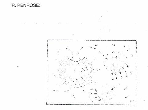
R. PENROSE:

Dynamical Collapse Theories : P. Pearle, Ghirardi -Rimini-Weber (GRW), L. Diosi, R. Penrose & recently S. Weinberg. (Rel Versions Bedingham , Tumulka, Pearle)Example, CSL: i) A modified Schrodinger equation, whosesolution is:

|ψ, t〉w = T e−∫ t

0 dt ′[

iH+ 14λ [w(t ′)−2λA]2

]|ψ,0〉. (1)

( T is the time-ordering operator). w(t) is a random classicalfunction of time, of white noise type, whose probability is givenby the second equation, ii) the Probability Rule:

PDw(t) ≡ w 〈ψ, t |ψ, t〉wt∏

ti =0

dw(ti)√2πλ/dt

. (2)

The processes U and R (corresponding to the observable A)are unified. For non-relativistic QM the proposal assumes :

A = ~X . Here λ must be small (no conflict with tests of QM) andbig enough ( rapid localization of “macroscopic objects”). GRWsuggested : λ ∼ 10−16sec−1

(Exp. bounds suggest λ(i) = λ(m(i)/mN)2).

We adapt the approach to situations involving both QuantumFields and Gravitation.

Dynamical reduction in uses the notion of “ time” ( the collapsetakes place in time).QG has a problem with time. Its resolution must involve passingto a sort of semiclassical regime. Our analysis assumes we canrely on a semiclassical framework.

Even if at the deepest levels gravitation must be quantummechanical in nature at the meso/macro scales, it correspondsto an emergent phenomena. Some traces of the quantumregime could survive in the form of an effective dynamical statereduction for matter fields.

Assume that if R << 1/l2Planck the description of gravitation interms of classical geometric notions would be justified,however, matter fields in general, might still require a quantumtreatment.

A word about pure, mixed, proper and improper states.

Take the view that individual isolated systems that are notentangled with others systems are represented by pure states.Mixed states occur when we consider either:a) “proper” An ensemble of (identical) systems each in a 6= purestate. (terminology borrowed from B. d’Espagnat)b) “improper” The state of a subsystem of a larger system(which is in a pure state), after we ” trace over” the rest of thesystem.An “proper ” (quantum) thermal state, (in statistical mechanics)represents an ensemble, with weights simple functions,characterized by temperature, and chemical potentials, etc .An ” improper” thermal state is a mixed state of type b) wherethe weights happen to be thermal.Resolving the BH information paradox requires explaining howa pure state becomes an proper (quantum) thermal state(rather than a ”improper ” one) : the inside region will simplydisappear!

To deal with all these issues, we make our analysis using a toymodel based on :

i) The CGHS black hole,

ii) A toy version of CSL adapted to QFT on CS,

iii) Some simple, and simplifying, assumptions about whathappens when QG cures a singularity, and

iv) An assumption that the CSL collapse parameter is not fixedbut depends (increases) with the local curvature.

Review of The Callan-Giddings-Harvey-Strominger (CGHS)model. The action :

S =1

2π

∫d2x√−g[e−2φ

[R + 4(∇φ)2 + 4Λ2

]− 1

2(∇f )2

],

(3)φ is the dilaton field, Λ2 a cosmological constant, and f is ascalar field (matter) .In the conformal gauge, using null coordinates:

ds2 = −e2ρdx+dx− (4)

The field f decouples and the general solution (KG Eq.) is

f (x+, x−) = f+(x+) + f−(x−). (5)

The solution corresponding to a left moving pulse of the field fis

ds2 = − dx+dx−

−Λ2x+x− − (M/Λx+0 )(x+ − x+

0 )Θ(x+ − x+0 ),

(0 ≤ x+ ≤ ∞,−∞ ≤ x− ≤ 0). (6)

Before the pulse, the solution corresponds to the, so called,linear dilaton vacuum solution and after x+

0 it turns into a blackhole solution.

It is useful to write the metric for the black hole region as

ds2 = − dx+dx−MΛ − Λ2x+(x− + ∆)

, (x+0 ≤ x+ ≤ ∞,−∞ ≤ x− ≤ 0)

(7)where ∆ = M/Λ3x+

0 .The Ricci curvature scalar has the form

R =4MΛ

M/Λ− Λ2x+(x− + ∆). (8)

The singularity corresponds to R =∞ (the locus of the zero inthe denominator).

The position of the event horizon ( D− (the singularity)) is givenby x− = −∆ = −M/Λ3x+

0 .

Besides these global coordinates, there are other usefulcoordinates in various regions.In the dilation vacuum region:

ds2 = −dy+dy−; −∞ < y− <∞; −∞ < y+ < 0 (9)

while in the BH exterior region one can use Schwarzschild likecoordinates (t , r ) so that,

ds2 =(−dt2 + dr2)

1 + (M/Λ)e−2rΛ(10)

Another set of Schwarzschild like coordinates to cover theinside horizon region

Field quantization Quantum Field Theory (QFT) constructionsfor f : uses the I−L and I−R as in region, and the black hole(exterior and interior) region as out region.In the in region the field operator can be expanded as

f (x) =∑ω

(aRωuR

ω + aR†ω uR∗

ω + aLωuL

ω + aL†ω uL∗

ω ). (11)

The mode- functions are positive energy ones ω > 0 for theregion . R and L mean right and left moving modes. Thatdefines an ”in vacuum R”(|0in〉R) and ”in-vacuum L” (|0in〉L)Then (|0in〉R ⊗ |0in〉L) is the ” in ” vacuum.

Instead of the usual plane wave modes we use a completeorthonormal set of localized wave packets modes uL/R

jn labeledby the integers j ≥ 0, n.

Expand the field in the out region in terms of the complete setof modes both outside (exterior) and inside (interior) the eventhorizon. The field operator has the form:

f (x) =∑ω

(bRω vR

ω + bR†ω vR∗

ω + bLωvL

ω + bL†ω vL∗

ω )+ (12)

∑ω

(ˆbRω vR

ω +ˆbR†ω vR∗

ω +ˆbLωvL

ω +ˆbL†ω vL∗

ω ) (13)

Tildes refer to the inside the horizon.

The relevant Bogolubov transformations are those in the rightmoving sector.

The transformation from in to exterior modes, which accountsfor the Hawking flux.

The point is that the initial state can be written ‘ ‘ at late times”as

|Ψin〉 = |0in〉R ⊗ |Pulse〉L = N∑Fnj

CFnj

∣∣Fnj⟩ext ⊗

∣∣Fnj⟩int ⊗ |Pulse〉L

(14)where a particle state Fnj consists of arbitrary but finite numberof particles.

If we traced over the interior DOF, we would end up with athermal state of type b) ( i.e. an improper one) correspondingto the Hawking flux.

limτ→τs

ρ(τ) = N2∑

F

e−2πΛ

EF |F 〉out ⊗ 〈F |out (15)

To apply the CSL theory, ( a modified time evolution of quantumstates of f ) we need a foliation of our space-time ( a “globaltime parameter”)

Use interaction-type picture: the free part of the evolutionencoded in the field operators, the interaction, ( the new CSLpart), in the evolution of the states.

In a relativistic context, based in a truly covariant version ofCSL, one would be using a Tomonaga-Schwinger typeinteraction picture evolution:

iδ |Ψ(Σ)〉 = HI(x)δ4x |Ψ(Σ)〉 (16)

change in the state tied to an infinitesimal deformation of thehypersurface with four volume δ4x around x in Σ.

The foliation we use ( has R = const. in the inside) and takesthe following form :

SINGULARITY

SINGULARITY

X

T

t = const.

r = const.

T = const.

Intersection Curves

I

II

III

The CSL collapse operator

The CSL equations can be generalized to drive collapse into astate of a joint eigen-basis of a set of commuting operators Aα

, [Aα,Aβ] = 0. For each Aα there will be one wα(t). In thiscase,we have

|ψ, t〉w = T e−∫ t

0 dt ′[

iH+ 14λ

∑α[wα(t ′)−2λAα]2

]|ψ,0〉. (17)

We call {Aα} the set of collapse operators. In this work wemake simplifying choices

i) States will collapse to a state of definite number of particles inthe inside region.

ii) We are working in the interaction picture which requires thereplacement H → 0 in the above equation.

The curvature dependent coupling λ in modified CSL

we assume that the CSL collapse mechanism will be amplifiedby the curvature of space-time: i .e. that the rate of collapse λ,will depend, in this case, of the Ricci scalar:

λ(R) = λ0

[1 +

(Rµ

)α](18)

where R is the Ricci scalar of the CGHS space-time and α > 1is a constant, µ provides an appropriate scale.In the region of interest we will have λ = λ(τ).

This evolution achieves, in the finite time to the singularity, whatordinary CSL achieves in infinite time, i.e. drives the state toone of the eigenstates of the collapse operators.

Thus the effect of CSL on the initial state:

|Ψin〉 = |0in〉R ⊗ |Pulse〉L = N∑Fnj

CFnj

∣∣Fnj⟩ext ⊗

∣∣Fnj⟩int ⊗ |Pulse〉L

(19)is to drive it to one of the eigenstates of joint the numberoperators. Thus at the hypersurfaces τ = Constant very closeto the singularity the state will be∣∣Ψin,τ

⟩= NCFnj

∣∣Fnj⟩ext ⊗

∣∣Fnj⟩int ⊗ |Pulse〉L (20)

No summation. Is a pure state. We do not know which one!

A role for quantum gravity: Assume that QG :a) : resolves the singularity and leads, on the other side, to areasonable space-time.b) : does not lead to large violations of the basic space-timeconservation laws.

Considering the “energetics” in the region just before thesingularity:

i) The Incoming positive energy flux corresponding to the leftmoving pulse that formed the BH.

ii) The incoming flux of the left moving vacuum state for the restof the modes which is known to be negative and essentiallyequal to the total Hawking Radiation flux.

iii) The flux associated with the right moving modes thatcrossed the collapsing matter but fell directly into the singularity.We know that the only thing missing here is the Hawkingradiation flux.

If energy is to be essentially conserved the post singularityregion must have a very small value of the energy. It might beassociated with some remnant radiation or perhaps a Plankmass remnant.

We ignore that, and replace it by the simplest thing: A zeroenergy momentum state corresponding to a trivial region ofspace-time.We denote it by

∣∣0post−singularity⟩.Thus, the evolution by assuming that the effects of QG can berepresented by the curing of the singularity and thetransformation:∣∣Ψin,τ

⟩= NCFnj

∣∣Fnj⟩ext ⊗

∣∣Fnj⟩int ⊗ |Pulse〉L

→ NCFnj

∣∣Fnj⟩ext ⊗

∣∣∣0post−singularity⟩

(21)

ENSEMBLES

We ended with a pure quantum state, but do not know whichone. That depends on the particular realization of the functionswα.Consider now an ensemble of systems prepared in the sameinitial state:

|Ψin〉 = |0in〉R ⊗ |Pulse〉L (22)

We describe this ensemble, by the pure density matrix:

ρ(τ0) = |Ψin〉 〈Ψin| (23)

Consider the CSL evolution of this density matrix up to thehypersurface just before the singularity.

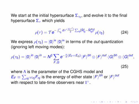
We start at the initial hypersurface Στ0 , and evolve it to the finalhypersurface Στ which yields

ρ(τ) = T e−∫ ττ0

dτ ′ λ(τ ′)2

∑nj [N

Lnj−NR

nj ]2ρ(τ0) (24)

We express ρ(τ0) = |0〉in 〈0|in in terms of the out quantization(ignoring left moving modes):

ρ(τ0) = |0〉in 〈0|in = N2∑F ,G

e−πΛ

(EF +EG) |F 〉bh ⊗ |F 〉out 〈G|bh ⊗ 〈G|out ,

(25)where Λ is the parameter of the CGHS model andEF ≡

∑nj ωnjFnj is the energy of either state |F 〉bh or |F 〉out

with respect to late-time observers near I+.

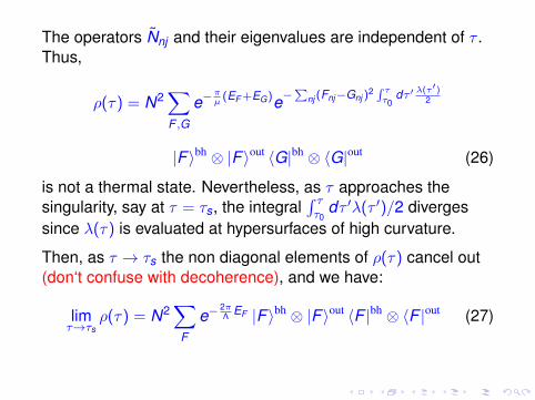
The operators Nnj and their eigenvalues are independent of τ .Thus,

ρ(τ) = N2∑F ,G

e−πµ

(EF +EG)e−∑

nj (Fnj−Gnj )2 ∫ τ

τ0dτ ′ λ(τ ′)

2

|F 〉bh ⊗ |F 〉out 〈G|bh ⊗ 〈G|out (26)

is not a thermal state. Nevertheless, as τ approaches thesingularity, say at τ = τs, the integral

∫ ττ0

dτ ′λ(τ ′)/2 divergessince λ(τ) is evaluated at hypersurfaces of high curvature.

Then, as τ → τs the non diagonal elements of ρ(τ) cancel out(don‘t confuse with decoherence), and we have:

limτ→τs

ρ(τ) = N2∑

F

e−2πΛ

EF |F 〉bh ⊗ |F 〉out 〈F |bh ⊗ 〈F |out (27)

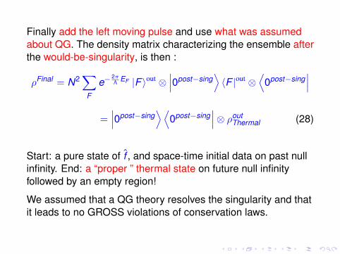
Finally add the left moving pulse and use what was assumedabout QG. The density matrix characterizing the ensemble afterthe would-be-singularity, is then :

ρFinal = N2∑

F

e−2πΛ

EF |F 〉out ⊗∣∣∣0post−sing

⟩〈F |out ⊗

⟨0post−sing

∣∣∣=∣∣∣0post−sing

⟩⟨0post−sing

∣∣∣⊗ ρoutThermal (28)

Start: a pure state of f , and space-time initial data on past nullinfinity. End: a “proper ” thermal state on future null infinityfollowed by an empty region!

We assumed that a QG theory resolves the singularity and thatit leads to no GROSS violations of conservation laws.

A this point, this is only a toy model, but we believe thatreasonable models with the same basic features would giveessentially the same picture, and thus represent an interestingpath to resolving the long standing conundrum known as the “Black Hole Information Loss Paradox”.

Singularity

Matter

Horizon

L R

RL

- -

++

Finally .. thinking of QG and virtual BH’s we obtain an attractive”boot-strap” picture... .... THANK YOU