Introduction to Black Hole Evaporation

PoS(Modave 2013)001

Introduction to Black Hole Evaporation

Pierre-Henry Lambert∗

Physique Théorique et MathématiqueUniversité Libre de Bruxelles and International Solvay InstitutesCampus Plaine C.P. 231, B-1050 Bruxelles, BelgiumE-mail: [email protected]

These lecture notes are an elementary and pedagogical introduction to the black hole evaporation,based on a lecture given by the author at the Ninth Modave Summer School in MathematicalPhysics and are intended for PhD students.First, quantum field theory in curved spacetime is studied and tools needed for the remaining ofthe course are introduced. Then quantum field theory in Rindler spacetime in 1+1 dimensions andin the spacetime of a spherically collapsing star are considered, leading to Unruh and Hawkingeffects, respectively. Finally some consequences such as thermodynamics of black holes andinformation loss paradox are discussed.

Ninth Modave Summer School in Mathematical Physics,1-7 September, 2013Modave, Belgium

∗Speaker.

c© Copyright owned by the author(s) under the terms of the Creative Commons Attribution-NonCommercial-ShareAlike Licence. http://pos.sissa.it/

mailto:[email protected]

PoS(Modave 2013)001

Introduction to Black Hole Evaporation Pierre-Henry Lambert

Contents

Introduction 3

1. Quantum Field Theory in curved spacetime 41.1 Quick review of QFT in flat spacetime 41.2 QFT in curved spacetime 6

1.2.1 Global hyperbolicity 61.2.2 QFT in globally hyperbolic spacetime 81.2.3 Stationary spacetime 9

1.3 Sandwhich spacetime 111.3.1 Bogoliubov gymnastics 121.3.2 Particle number 13

2. Quantum Field Theory in Rindler spacetime in 1+1 dimensions – Unruh effect 142.1 Rindler spacetime in 1+1 dimensions 142.2 Quantization 162.3 Unruh effect 16

2.3.1 Fun with integrals 182.3.2 Thermal bath 19

3. Quantum Field Theory in spacetime of spherically collapsing star – Hawking effect 203.1 The set-up 203.2 Wave equation 213.3 Geometric optics approximation 233.4 Hawking’s computation 23

4. Some consequences of Hawking radiation 264.1 Thermodynamics of black holes 26

4.1.1 Surface gravity 264.1.2 Some properties of κ 274.1.3 The laws 29

4.2 Information loss paradox and black hole complementarity 29

Acknowledgments 30

2

PoS(Modave 2013)001


Introduction

There are several reasons for which the general relativity theory cannot be the final theory inorder to describe the gravitational interaction. From one side the theory predicts the existence ofsingularities but does not resolve them, this is clearly an internal evidence that general relativitytheory is incomplete. On the other side, general relativity is a classical theory but Nature is funda-mentally quantum (in a certain sense) and at present a quantum theory of gravity is still missing.This is an external evidence that general relativity cannot be the final theory concerning gravity.

Even though a theory of quantum gravity is not available, one can nevertheless try to gain someinformation about the quantum properties of gravity by using an approximation scheme. A schemeone can consider is the semi-classical theory in which the gravity is treated classically but on whichquantum fields can propagate. In this approximation scheme, the quantum fields satisfy their usualequations of motion but with the usual Minkowski constant metric replaced by the classical metricof the curved spacetime under consideration.

The main aim of this lecture notes is to present, in a very basic and (hopefully) pedagogicalway, the surprising result discovered by Hawking [1] in which black holes are shown to create andemit particles in the semi-classical approach when quantum effects are taken into account, contraryto the prediction of the classical theory. These notes are based on a lecture that was given by theauthor at the Ninth Modave Summer School in Mathematical Physics and was intended for PhDstudents that are not necessarily familiar with quantum field theory in curved spacetimes. Emphasisis put in such a way of providing a very pedestrian and elementary introduction about this topicwith no other ambition than being as self-contained as possible. Some standard notions of generalrelativity are supposed to be known, in particular the notions of black holes and Carter-Penrosediagrams. These lecture notes are so pitched that graduate students familiar with these notionsshould have essentially no difficulty in following it.

In practice, these notes are mainly based on the original paper of Hawking [1], on the generalrelativity book of Carroll [4] and on the notes on black holes of Townsend [5] and Dowker [6].Interested readers are warmly invited to consult some other references such as the book of Birrelland Davies [2] from the eighties, or the one of Wald [3] from the nineties or the more recent one ofMukhanov and Winitski [13].

These lecture notes are organized as follow. In the first section, general properties of quantumfield theory in curved spacetime are studied and differences with respect to flat space are pointedout. Then applications of the formalism are considered. First in the case of a sandwhich spacetimebefore considering the more physically interesting case of Rindler space in 1+1 dimensions andalso the spacetime of a spherically collapsing star. This will lead to Unruh and Hawking effects,respectively. Finally some consequences of the result of Hawking are discussed, namely the ther-modynamics of black holes and the information loss paradox. Several figures are included, in orderto make the presentation of the topic more pedagogical.

Any comments about these lecture notes are welcome.

3

PoS(Modave 2013)001


1. Quantum Field Theory in curved spacetime

1.1 Quick review of QFT in flat spacetime

The signature is taken to be (−,+,+,+) throughout the lecture. Consider the following action[4][6]

S =∫

d4x L , with L =−12

∂µφ∂µ

φ − 12

m2φ

2. (1.1)

The equation of motion, obtained by requiring the action to be stationary, read

δS = 0 ⇒ φ −m2φ = 0, (1.2)

where = ∂µ∂ µ . Equation (1.2) is the familiar Klein-Gordon equation. The conjugate momentumis defined by π = ∂L

∂∂0φ= φ , where φ = ∂tφ .

A set of solutions to the Klein-Gordon equation of motion is given by plane waves,

f = f0eikµ xµ

, (1.3)

with kµ = (ω,ki),kµ = (−ω,ki) where ω is the frequency and ki the wave vector. In the rest ofthe lecture, the wave vector ki will be denoted by k, except when explicitely stated. The dispersionrelation is obtained by replacing the plane wave solution (1.3) into the Klein-Gordon equation (1.2),

ω2 = k2 +m2, (1.4)

with k2 = kiki. This relation means that the wave vector k completely determines the frequency ω ,up to a sign. The frequency ω is chosen to be a positive number and so the set of solutions (1.3)becomes parameterized by the wave vector k:

fk = f0eikµ xµ

. (1.5)

By definition, modes fk such that

∂t fk =−iω fk, with ω > 0, (1.6)

are called positive frequency modes. Similarly, modes f ∗k such that

∂t f ∗k = iω f ∗k , with ω > 0, (1.7)

are called negative frequency modes (even though ω is positive). One can ask why the positivemodes are written like this and the answer is that it will be easier to generalize this notion later onwhen quantum field theory will be considered in curved spacetime.

In order to have a complete and orthonormal set of modes, an inner product must be definedon the space of solutions of the Klein-Gordon equation of motion. The inner product between twosolutions f an g is defined by

( f ,g) =−i∫

d3x ( f ∂tg∗−g∗∂t f ). (1.8)

4

PoS(Modave 2013)001


The normalization of the set of modes is obtained by considering the inner product between twoplane waves fk1 = e−iω1t+ik1x and fk2 = e−iω2t+ik2x,

( fk1 , fk2) =−i∫

d3x i(ω1 +ω2)e−i(ω1−ω2)tei(k1−k2)x,

= (ω1 +ω2) δ3(k1− k2)(2π)3e−i(ω1−ω2)t , (1.9)

where the definition of the delta distribution was used, i.e. δ 3(k1− k2) =∫ d3x

(2π)3 ei(k1−k2)x. From(1.9) one can see that the inner product between two different sets of modes vanishes unless thetwo wave vectors k1,k2 (and thus the corresponding frequency, by the dispersion relation) are equal.The set of modes (1.5) can then be normalized as

fk =1

(2π)3/2

1√2ω

eikµ xµ

. (1.10)

This normalization implies the relations

( fk, fk′) = δ (k− k′), ( fk, f ∗k′) = 0, ( f ∗k , f ∗k′) =−δ (k− k′). (1.11)

Any classical field configuration φ(x) that is solution to the Klein-Gordon equation can be ex-panded in terms of the basis modes f , f ∗,

φ(x) =∫

d3k (ak fk +a∗k f ∗k ), (1.12)

where ak and a∗k are some coefficients with respect to the basis modes in the expansion of the fieldconfiguration.

The scalar field can be canonically quantized, by replacing the classical fields by operatorsacting on Hilbert space and by imposing the canonical commutation relation

[φ(t,x),π(t,x)] = δ (x− x′). (1.13)

After quantization, the classical field φ expanded in terms of modes becomes the following operator

φ =∫

d3k (ak fk +a†k f ∗k ). (1.14)

Note that the operator ak in the expansion of the quantum field φ was defined at the classical levelto be the coefficient of the positive frequency mode. This fact seems anecdotic right now but willhowever play an important role later on when quantum field theory will be considered in curvedspacetime. From the commutation relation (1.13) and the field expansion (1.14) one can easilycheck that the operators ak,a

†k satisfy

[ak,a†k′ ] = δ (k− k′). (1.15)

Relation (1.15) is exactly the same relation as for the creation/annihilation operators of the familiarquantum harmonic oscillator, except that there is one oscillator for each mode k. As for the har-monic oscillator, the vacuum is defined to be the state |0〉 such that ak|0〉= 0, ∀k, and the numberof particles of momentum k is defined by operator Nk = a†

kak, with no k summation in the righthand side.

5

PoS(Modave 2013)001


1.2 QFT in curved spacetime

Let us move to curved spacetime by choosing some background (M,g). Suppose that (M,g)is globally hyperbolic. What does that mean?

1.2.1 Global hyperbolicity

In this section, based on [5], [6], [7], [8], [9] and [10] the notion of global hyperbolicity isconsidered. First some definitions are needed.

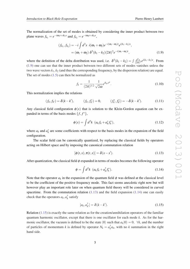
DEFINITION 1The future domain of dependence of a hypersurface Σ, denoted by D+(Σ), is the set of points p∈Mfor which every past (inextendable) causal curves through p intersect Σ.

This definition is illustrated by figures 1 and 2.

Figure 1: Past causal curve throught point p. Figure 2: The future domain of dependence of Σ.

In the case of partial differential equation, the meaning of this notion is that the behavior of thesolution of the partial differential equation outside D+(Σ) is not determined by initial data on Σ.

DEFINITION 2The past domain of dependence of a hypersurface Σ, denoted by D−(Σ), is the set of points p ∈Mfor which every future (inextendable) causal curves through p intersect Σ.

DEFINITION 3Σ is said to be a Cauchy surface for (M,g) if D+(Σ)

⋃D−(Σ) = M.

DEFINITION 4(M,g) is globally hyperbolic if there exists (at least) one Cauchy surface Σ for (M,g).

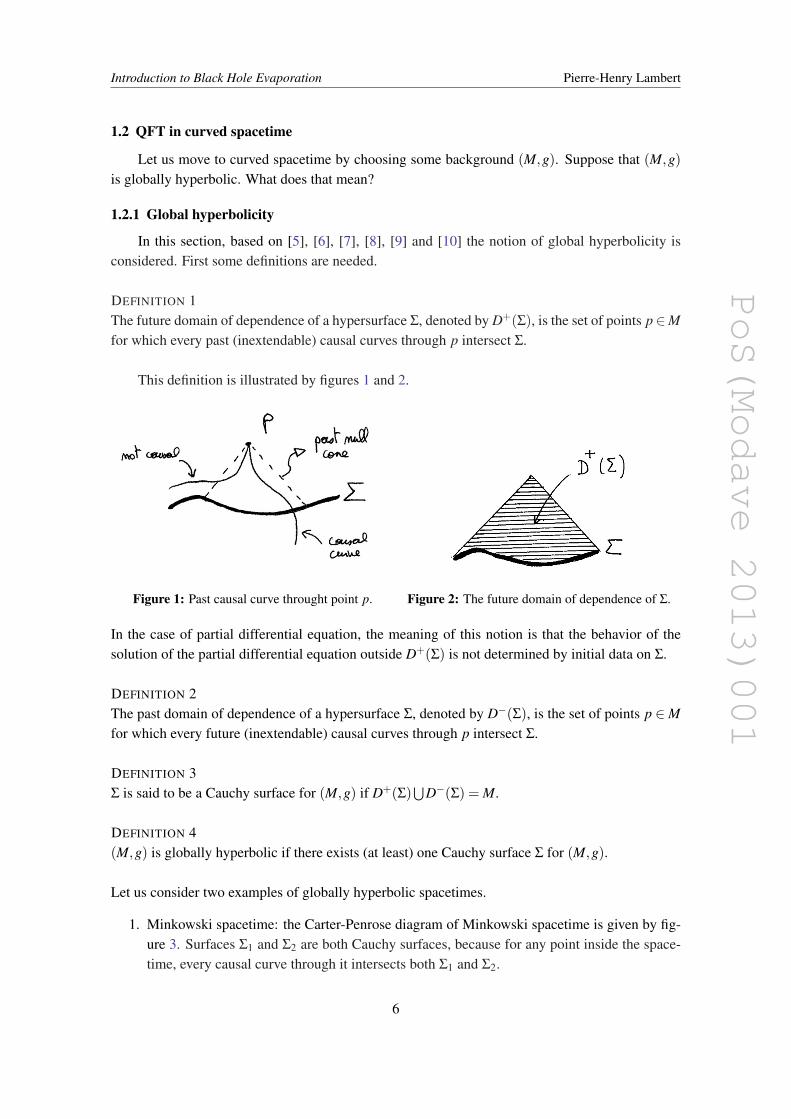
Let us consider two examples of globally hyperbolic spacetimes.

1. Minkowski spacetime: the Carter-Penrose diagram of Minkowski spacetime is given by fig-ure 3. Surfaces Σ1 and Σ2 are both Cauchy surfaces, because for any point inside the space-time, every causal curve through it intersects both Σ1 and Σ2.

6

PoS(Modave 2013)001


Figure 3: Carter-Penrose diagram for Minkowski. Figure 4: Carter-Penrose diagram for Kruskal.

2. Kruskal spacetime (the maximal analytic extension of Schwarzschild): The Carter-Penrosediagram of Kruskal spacetime is given by figure 4. Again Σ1 and Σ2 are Cauchy surfaces.

In the case where the spacetime (M,g) is not globally hyperbolic, then either D+(Σ) or D−(Σ) hasa boundary on M.

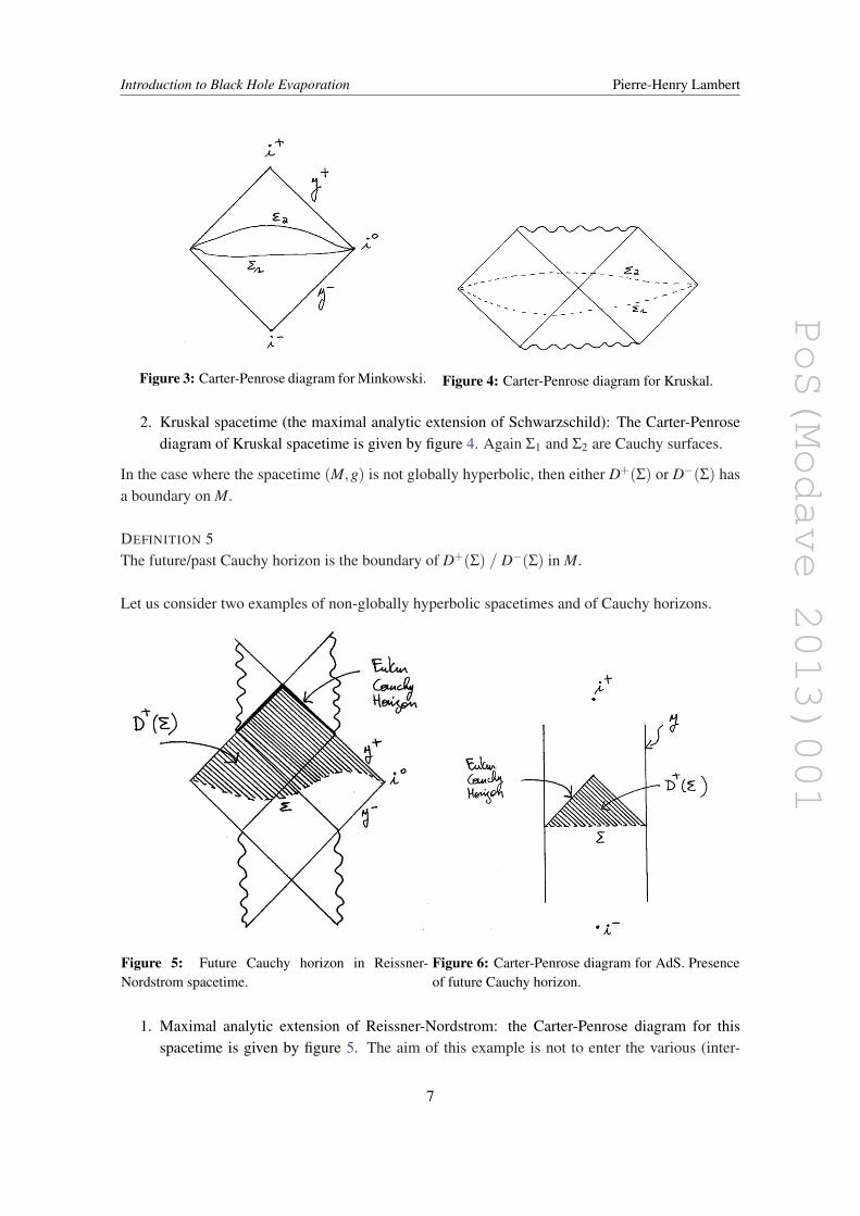
DEFINITION 5The future/past Cauchy horizon is the boundary of D+(Σ) / D−(Σ) in M.

Let us consider two examples of non-globally hyperbolic spacetimes and of Cauchy horizons.

Figure 5: Future Cauchy horizon in Reissner-Nordstrom spacetime.

Figure 6: Carter-Penrose diagram for AdS. Presenceof future Cauchy horizon.

1. Maximal analytic extension of Reissner-Nordstrom: the Carter-Penrose diagram for thisspacetime is given by figure 5. The aim of this example is not to enter the various (inter-

7

PoS(Modave 2013)001


esting) details of this spacetime, but instead to illustrate the notion of Cauchy horizon fornon-globally hyperbolic spacetime.

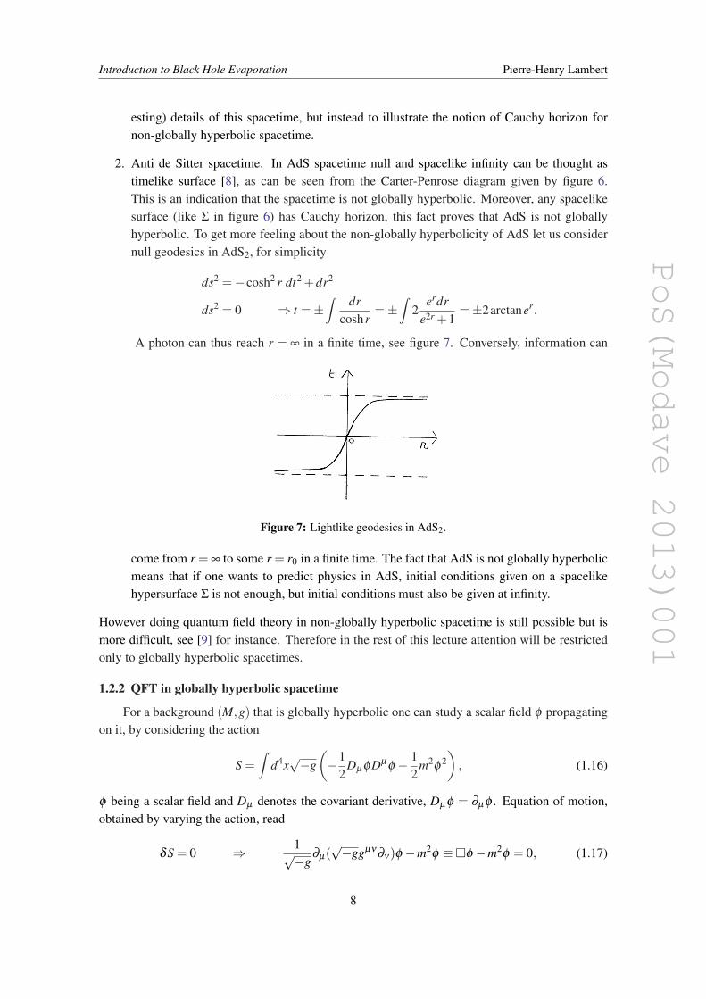
2. Anti de Sitter spacetime. In AdS spacetime null and spacelike infinity can be thought astimelike surface [8], as can be seen from the Carter-Penrose diagram given by figure 6.This is an indication that the spacetime is not globally hyperbolic. Moreover, any spacelikesurface (like Σ in figure 6) has Cauchy horizon, this fact proves that AdS is not globallyhyperbolic. To get more feeling about the non-globally hyperbolicity of AdS let us considernull geodesics in AdS2, for simplicity

ds2 =−cosh2 r dt2 +dr2

ds2 = 0 ⇒ t =±∫ dr

coshr=±

∫2

erdre2r +1

=±2arctaner.

A photon can thus reach r = ∞ in a finite time, see figure 7. Conversely, information can

Figure 7: Lightlike geodesics in AdS2.

come from r = ∞ to some r = r0 in a finite time. The fact that AdS is not globally hyperbolicmeans that if one wants to predict physics in AdS, initial conditions given on a spacelikehypersurface Σ is not enough, but initial conditions must also be given at infinity.

However doing quantum field theory in non-globally hyperbolic spacetime is still possible but ismore difficult, see [9] for instance. Therefore in the rest of this lecture attention will be restrictedonly to globally hyperbolic spacetimes.

1.2.2 QFT in globally hyperbolic spacetime

For a background (M,g) that is globally hyperbolic one can study a scalar field φ propagatingon it, by considering the action

S =∫

d4x√−g(−1

2DµφDµ

φ − 12

m2φ

2), (1.16)

φ being a scalar field and Dµ denotes the covariant derivative, Dµφ = ∂µφ . Equation of motion,obtained by varying the action, read

δS = 0 ⇒ 1√−g

∂µ(√−ggµν

∂ν)φ −m2φ ≡φ −m2

φ = 0, (1.17)

8

PoS(Modave 2013)001


where φ is defined to be the first term in the left hand side of (1.17). This is the usual Klein-Gordon equation.The inner product on solutions space of the Klein-Gordon equation is defined by

(φ1,φ2) =−i∫

Σ

d3x√

γ nµ (φ1Dµφ∗2 −φ

∗2 Dµφ1), (1.18)

where Σ is a Cauchy surface1, with normal vector nµ and induced metric γ . This inner productis natural, i.e. is independent of the choice of the Cauchy surface Σ. Indeed, by considering twodifferent Cauchy surfaces Σ1 and Σ2, we have

(φ1,φ2)|Σ1− (φ1,φ2)|Σ2 =−i∫

Ω=Σ1−Σ2

d3x√

γ nµ (φ1Dµφ∗2 −φ

∗2 Dµφ1),

=−i∫

∂Ω

d4x√−g Dµ(φ1Dµφ

∗2 −φ

∗2 Dµφ1),

=−i∫

∂Ω

d4x√−g (φ1m2

φ∗2 −φ

∗2 m2

φ1) = 0,

where Stokes theorem and the equation of motion were used to get the second and third lines, re-spectively. This inner product allows to have an (a priori non-unique) orthonormal basis satisfying

( fi, f j) = δi j, ( f ∗i , f ∗j ) =−δi j, (1.19)

where indices i, j, . . . can be discrete or continuous. In order to make things as easy as possible, thenotation for the discrete case is adopted. This inner product allows to define an orthonormal basis,but this basis is non-unique and after canonical quantization of the theory there will be differentnotions of vacuum, according to each different orthonormal basis. This is because there is nopreferred time coordinate in curved spacetime, except if another assumption is made.

1.2.3 Stationary spacetime

The assumption that is made on the spacetime (M,g) is stationary symmetry.

DEFINITION 6A spacetime (M,g) is stationary if there exists a timelike killing vector field K = Kµ∂µ for themetric g, i.e. LKg = 0.

This definition implies that there exists a coordinate system xµ such that the metric is timeindependent, i.e. ∂tgµν = 0. Indeed, in an arbitrary coordinate system the Killing equation is

0 = LKgµν ≡ Kσ∂σ gµν +gσν∂µKσ +gµσ ∂νKσ , (1.20)

and choosing a coordinate system xµ in which Kµ = (1,0,0,0) reduces (1.20) to ∂tgµν = 0,hence the result. Roughly speaking, or at least intuitively, stationary means time independent.

So far so good. The globally hyperbolic background (M,g) is stationary, with a Killing vectorfield K. This Killing vector field enjoys two properties.

1This is the place where global hyperbolicity hypothesis is important.

9

PoS(Modave 2013)001


1. First of all, it commutes with the Klein-Gordon operator −m2. Indeed, from one side wehave

∂tφ = ∂t(Dµgµν∂νφ) = gµν

∂t(∂µ∂νφ −Γσµν∂σ φ) = gµν(∂t∂µ∂νφ −Γ

σµν∂t∂σ φ),

because of stationary symmetry the metric (and hence the Christoffel symbols) are timeindependent. On the other side, we have

∂tφ = Dµgµν∂ν(∂tφ) = gµν(∂µ∂ν∂tφ −Γ

σµν∂σ (∂tφ)),

which shows the result. Note that the action of a vector field on a function is still a function,i.e. LKφ = Kµ∂µφ , and in the coordinate system in which Kµ = (1,0,0,0) this actionreduces to LKφ = ∂tφ but the result remains a function and not a vector field.

2. The second property of the Killing vector field K = ∂µ is antihermiticity. Indeed,

( f ,Kg) =−i∫

Σ

d3x√

γ nµ( f Dµ(∂tg∗)− (∂tg∗)Dµ f ),

=−i∫

Σ

d3x√

γ nµ((−∂t f )Dµg∗−g∗Dµ(−∂t f )),

= (−K f ,g),

where integration by parts was used in the second line. Since the operator K is antihermitian,its eigenvalues are purely imaginary, i.e. K f j =−iω f j, for some real ω .

This property of having purely imaginary eigenvalues is used to define the notion of positive fre-quency modes in the case of curved spacetime. If

LK f j ≡ ∂t f j =−iω f j, ω > 0, (1.21)

then the modes f j are called positive frequency modes. In the same way for modes f ∗j , i.e. if

LK f ∗j ≡ ∂t f ∗j = iω f ∗j , ω > 0, (1.22)

then the modes f ∗j are called negative frequency modes.The theory can be quantized, exactly in the same way as in flat space, namely by replacing

classical fields by operators acting on Hilbert space, and by imposing canonical commutation re-lations between the operators. Any field configuration φ(x) that is solution to the Klein-Gordonequation can be expanded with respect to the basis

φ(x) = ∑i

ai fi +a†i f ∗i . (1.23)

To make things as simple as possible, the discrete notation is chosen. Again, the operators infront of positive and negative frequency modes in the field expansion are the creation/annihilationoperators satisfying the commutation relation [ak,a

†k′ ] = δ (k− k′). The vacuum state is defined to

be the state |0〉 such that ak|0〉 = 0, ∀k. In conclusion, stationary symmetry alows to pick up apreferred time coordinate, given by the timelike Killing vector field.

This is the end of the general formalism of quantum field theory in curved spacetime. In therest of the lecture, applications of it will be considered.

10

PoS(Modave 2013)001


1.3 Sandwhich spacetime

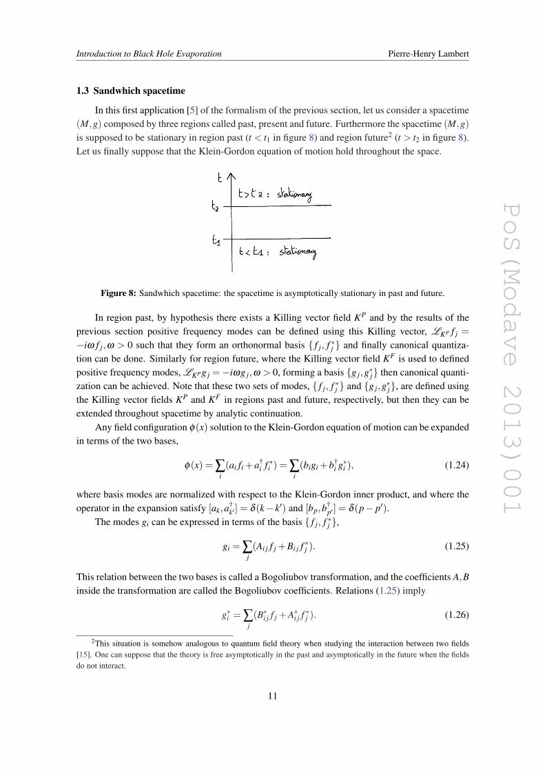
In this first application [5] of the formalism of the previous section, let us consider a spacetime(M,g) composed by three regions called past, present and future. Furthermore the spacetime (M,g)is supposed to be stationary in region past (t < t1 in figure 8) and region future2 (t > t2 in figure 8).Let us finally suppose that the Klein-Gordon equation of motion hold throughout the space.

Figure 8: Sandwhich spacetime: the spacetime is asymptotically stationary in past and future.

In region past, by hypothesis there exists a Killing vector field KP and by the results of theprevious section positive frequency modes can be defined using this Killing vector, LKP f j =

−iω f j,ω > 0 such that they form an orthonormal basis f j, f ∗j and finally canonical quantiza-tion can be done. Similarly for region future, where the Killing vector field KF is used to definedpositive frequency modes, LKPg j =−iωg j,ω > 0, forming a basis g j,g∗j then canonical quanti-zation can be achieved. Note that these two sets of modes, f j, f ∗j and g j,g∗j, are defined usingthe Killing vector fields KP and KF in regions past and future, respectively, but then they can beextended throughout spacetime by analytic continuation.

Any field configuration φ(x) solution to the Klein-Gordon equation of motion can be expandedin terms of the two bases,

φ(x) = ∑i(ai fi +a†

i f ∗i ) = ∑i(bigi +b†

i g∗i ), (1.24)

where basis modes are normalized with respect to the Klein-Gordon inner product, and where theoperator in the expansion satisfy [ak,a

†k′ ] = δ (k− k′) and [bp,b

†p′ ] = δ (p− p′).

The modes gi can be expressed in terms of the basis f j, f ∗j ,

gi = ∑j(Ai j f j +Bi j f ∗j ). (1.25)

This relation between the two bases is called a Bogoliubov transformation, and the coefficients A,Binside the transformation are called the Bogoliubov coefficients. Relations (1.25) imply

g∗i = ∑j(B∗i j f j +A∗i j f ∗j ). (1.26)

2This situation is somehow analogous to quantum field theory when studying the interaction between two fields[15]. One can suppose that the theory is free asymptotically in the past and asymptotically in the future when the fieldsdo not interact.

11

PoS(Modave 2013)001


These Bogoliubov transformations can be written in a matrix form,(gg∗

)=

(A BB∗ A∗

)(ff ∗

). (1.27)

1.3.1 Bogoliubov gymnastics

In order to invert relation (1.27) easily, some relations between the Bogoliubov coefficients areneeded. Let us make some gymnastics with them.The basis is normalized in such a way that (α f ,βg) = αβ ∗( f ,g) see (1.18), so we have

(gi,g j) = δi j

= (Aip fp +Bip f ∗p ,A jq fq +B jq f ∗q )

= AipA∗jp +BiqB∗jq(−1) = AipA†p j−BipB†

p j.

Hence the relation

AA†−BB† = 1. (1.28)

From the basis orthonormalization, we also have

(gi,g∗j) = 0

= (Aip fp +Bip f ∗p ,B∗jq fq +A∗jq f ∗q )

= AipB jp +BiqA jq(−1) = AipAtp j−BipAt

p j.

Thus,

ABt −BAt = 0. (1.29)

Relation (1.28)(1.29) between Bogoliubov coefficients allow to invert the matrix M =

(A BB∗ A∗

)present in (1.27) easily. The inverse is given by

M−1 =

(A BB∗ A∗

)−1

=

(A† −Bt

−B† At

). (1.30)

Indeed, we have

M−1M =

(AA†−BB† −ABt +BAt

B∗A†−A∗B† −B∗Bt +A∗At

)=

(1 00 1

).

The field expansion (1.24) can be written in a matrix form,

φ =(

b b†)( g

g∗

)=(

a a†)( f

f ∗

), (1.31)

12

PoS(Modave 2013)001


and using the Bogoliubov transformations (1.25) and (1.30) we have(gg∗

)=

(A BB∗ A∗

)(ff ∗

),

(ff ∗

)=

(A† −Bt

−B† At

)(gg∗

). (1.32)

So the field expansion (1.31) becomes

(b b†

)( gg∗

)=(

a a†)( A† −Bt

−B† At

)(gg∗

), (1.33)

which gives the relation (bb†

)=

(A∗ −B∗

−B A

)(aa†

). (1.34)

This relation between the creation/annihilation operators with respect to the two different basesends the Bogoliubov gymnastics part. Let us go back to physics.

1.3.2 Particle number

The vacuum associated to modes fi, f ∗i , called the in vacuum, |in〉, is defined such thatai|in〉 = 0,∀i. Now the following question can be considered: what is the expected number ofparticles of species i present in the state |in〉when evaluated by stationary observer in region future?Let us compute this number.

Ni = 〈in|FNi|in〉= 〈in|b†i bi|in〉,

= 〈in|(−Bipap +Aipa†p)(A

∗iqaq−B∗iqa†

q)|in〉,= 〈in|BiqB∗ipδpq|in〉= BipB†

pi.

The number of particles is given by

Ni = (BB†)ii , (1.35)

where there is no i summation. So at the end one can see that the number of particles is just givenby the Bogoliubov coefficient. And, in general, this coefficient is non-zero3. The total number ofparticles of all species is obtained by summing over all the species, i.e. N = ∑i Ni = Tr(BB†).

3This number is always zero in the case of unitary Bogoliubov transformation (1.25) as can be seen from (1.28), i.e.B = 0⇒ AA† = 1.

13

PoS(Modave 2013)001


2. Quantum Field Theory in Rindler spacetime in 1+1 dimensions – Unruh effect

In this part, quantum field theory in Rindler space [4] is studied. Many aspects will be relevantfor the discussion of Hawking radiation later on. Quantum field theory in Rindler space meansquantization carried out by an accelerating observer in Minkowski space. This will lead to theUnruh effect4. To evoid all possible complications, the quantum field theory is considered assimple as it can be, without becoming completely trivial, i.e. we consider a massless scalar field intwo dimensions. The action is

S =∫

d2x − 12

∂µφ∂µ

φ (2.1)

from which the equations of motion read δS = 0⇒ φ = 0. Before quantizing the theory, let usspend some time studying Minkowski spacetime in two dimensions from the point of view of anaccelerating observer.

2.1 Rindler spacetime in 1+1 dimensions

By definition, Rindler spacetime is a sub-region of Minkowski spacetime (ds2 =−dt2 +dx2)associated with an observer that is eternally accelerating at constant rate. The parametric motion(i.e. the trajectory) of such an observer is given by

x(τ) =1α

cosh(ατ), (2.2)

t(τ) =1α

sinh(ατ), (2.3)

where α is a constant parameter. The acceleration is given by

aµ =D2xµ

dτ2 =d2xµ

dτ2 = (α sinh(ατ),α cosh(ατ)),

a2 = aµaνgµν = α2, (2.4)

and one can see that the acceleration is constant, a = ±α , as it should. The world line of the ob-server xµxµ satisfies −t2 + x2 = 1

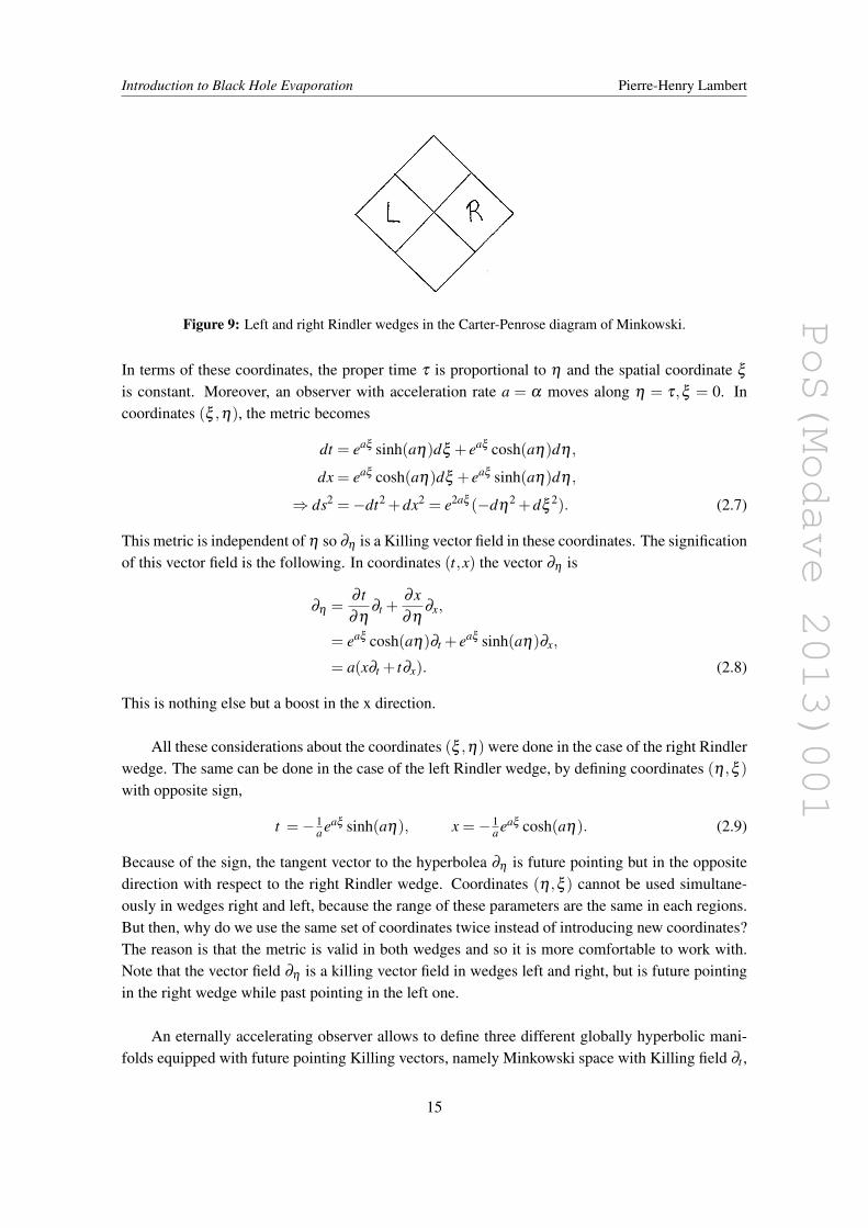
α2 . This is an hyperbolic motion and lines x = t are the horizonsfor this observer because region x≤ t is forever forbidden to a Rindler observer.In terms of the Carter-Penrose diagram of Minkowski space, the observer only covers two parts ofit, called the Rindler wedges, the left one and right one, see figure 9.

Instead of using coordinates (t,x), let us introduce some new coordinates (η ,ξ ) more fitted tothe description of the accelerated motion in the right Rindler wedge,

t =1a

eaξ sinh(aη), x =1a

eaξ cosh(aη), (2.5)

η =α

aτ, ξ =

1a

lnα

a. (2.6)

4Historically Unruh effect was discovered after Hawking radiation in order to better understand it. But as this lectureis not a lecture about history of physics, Unruh effect will be considered first, before Hawking effect.

14

PoS(Modave 2013)001


Figure 9: Left and right Rindler wedges in the Carter-Penrose diagram of Minkowski.

In terms of these coordinates, the proper time τ is proportional to η and the spatial coordinate ξ

is constant. Moreover, an observer with acceleration rate a = α moves along η = τ,ξ = 0. Incoordinates (ξ ,η), the metric becomes

dt = eaξ sinh(aη)dξ + eaξ cosh(aη)dη ,

dx = eaξ cosh(aη)dξ + eaξ sinh(aη)dη ,

⇒ ds2 =−dt2 +dx2 = e2aξ (−dη2 +dξ

2). (2.7)

This metric is independent of η so ∂η is a Killing vector field in these coordinates. The significationof this vector field is the following. In coordinates (t,x) the vector ∂η is

∂η =∂ t∂η

∂t +∂x∂η

∂x,

= eaξ cosh(aη)∂t + eaξ sinh(aη)∂x,

= a(x∂t + t∂x). (2.8)

This is nothing else but a boost in the x direction.

All these considerations about the coordinates (ξ ,η) were done in the case of the right Rindlerwedge. The same can be done in the case of the left Rindler wedge, by defining coordinates (η ,ξ )

with opposite sign,

t =−1a eaξ sinh(aη), x =−1

a eaξ cosh(aη). (2.9)

Because of the sign, the tangent vector to the hyperbolea ∂η is future pointing but in the oppositedirection with respect to the right Rindler wedge. Coordinates (η ,ξ ) cannot be used simultane-ously in wedges right and left, because the range of these parameters are the same in each regions.But then, why do we use the same set of coordinates twice instead of introducing new coordinates?The reason is that the metric is valid in both wedges and so it is more comfortable to work with.Note that the vector field ∂η is a killing vector field in wedges left and right, but is future pointingin the right wedge while past pointing in the left one.

An eternally accelerating observer allows to define three different globally hyperbolic mani-folds equipped with future pointing Killing vectors, namely Minkowski space with Killing field ∂t ,

15

PoS(Modave 2013)001


right Rindler wedge with Killing field ∂η and left Rindler wedge with future pointing Killing field−∂η . Let us proceed to canonical quantization of the scalar field in Minkowski space and then inthe right Rindler wedge.

2.2 Quantization

• In Minkowski spacetime, the equation of motion read φ = (−∂ 2t + ∂ 2

x )φ = 0 and admitsplane waves solutions,

fk =1√

4πωeikµ xµ

, kµ = (ω,k). (2.10)

Positive frequency modes are defined with respect to Killing vector field ∂t , i.e. by the con-dition ∂t fk =−iω fk,ω > 0. After canonical quantization, any field configuration φ solutionto the equation of motion can be expanded in terms of fk, f ∗k ,

φ = ∑k(ak fk +a†

k f ∗k ). (2.11)

The vacuum is defined by state |0〉 such that ak|0〉= 0,∀k.

• In the right Rindler wedge, the equation of motion read φ = e−2aξ (−∂ 2η + ∂ 2

ξ)φ = 0 and

admits plane wave solutions,

gRk =

1√4πω

eikµ xµ

, xµ = (η ,ξ ). (2.12)

Positive frequency modes are defined with respect the the Killing vector field ∂η , i.e. by thecondition ∂ηgR

k = −iωgRk ,ω > 0. After canonical quantization, any field φ solution to the

field equation can be expanded in terms of gRk ,g

R∗k ,

φ = ∑k(bkgR

k +b†kbR∗

k ), (2.13)

and the vacuum is defined by state |R0〉 such that bk|R0〉= 0,∀k.

2.3 Unruh effect

Now the physically interesting question arrives: what does an observer in the right Rindlerwedge see in the Minkowski vacuum?

Some care must be taken because the Rindler modes gRk are not defined on a Cauchy surface

for the whole Minkowski space. These modes are only defined on a Cauchy surface for the caseof manifold being the right Rindler wedge, and so these modes are not complete with respect toMinkowski spacetime. This is not really a problem because global modes can be defined,

gRk =

1√

4πωeikµ xµ

in right Rindler wedge

0 in left Rindler wedge(2.14)

These modes are defined on an entire Cauchy surface (η = 0 for instance), but they are not com-plete. Positive frequency modes need to be introduced in the left wedge, and are defined by

gLk =

0 in right Rindler wedge

1√4πω

eikµ xµ

in left Rindler wedge(2.15)

16

PoS(Modave 2013)001


These modes are positive frequency modes with respect to Killing vector field −∂η .

Taken together, gRk ,g

R∗k and gL

k ,gL∗k form a complete set of modes for the Minkowski

space, and thus there are two possible modes expansions for any field configuration solution to theequation of motion,

φ = ∑k(bkgR

k + ckgLk +h.c.), (2.16)

φ = ∑k(ak fk +h.c.). (2.17)

Now one can wonder how many right particules are expected to be seen in Minkowski vacuum,or equivalently what does the eternally accelerating observer see in the Minkowski vacuum whilebeing in the right Rindler wedge. Mathematically the question is

〈0Mink|RNk|0Mink〉= ?

There is a relation between modes gRk and fk, given by the Bogoliubov transformation5,

gRk (u) =

∫dω′(Aωω ′ fω ′+Bωω ′ f ∗ω ′). (2.18)

Recall that fω ′ =1√

4πω ′eikµ xµ

and ikµxµ = −iω ′t + ikx = −iω ′(t− x) = −iω ′u with u = t− x. Sothe Bogoliubov transformation relating the bases (2.18) becomes

gRk (u) =

∫dω′(

Aωω ′1

2π

√π

ω ′e−iω ′u +Bωω ′

12π

√π

ω ′eiωu

). (2.19)

This expression for gRk (u) looks like the inverse Fourier transform of gR

k (u). Indeed,

gRk (u) =

12π

∫ +∞

−∞

dω′e−iω ′ugω(ω

′), (2.20)

where gω(ω′) is the Fourier transform of gR

k (u), i.e. gω(ω′) =

∫ +∞

−∞dueiω ′ugR

k (u). Equation (2.20)can also be re-written as

gRk (u) =

12π

∫ +∞

0dω′e−iω ′ugω(ω

′)+1

2π

∫ +∞

0dω′eiω ′ugω(−ω

′), (2.21)

where the values of integration and also the variable of integration were changed in the second term.By comparing this expression (2.21), i.e. the expression for the inverse Fourier transform of thefunction gR

k (u), with the expression (2.18), i.e. the expression for the Bogoliubov transformationof the function gR

k (u), one can get an expression for the Bogoliubov coefficient,

Aωω ′ =

√ω ′

πgω(ω

′), Bωω ′ =

√ω ′

πgω(−ω

′). (2.22)

Recall the relation AA†−BB† = 1 from the Bogoliubov gymnastics (1.28), which is equivalent to|A|2−|B|2 = 1. So if there exists also a relation between g(−ω ′) and g(ω ′) then the Bogoliubovcoefficient |B|2 will be immediately known without other computation.

The desired relation between functions g(−ω ′) and g(ω ′) is given by

g(−ω′) =−e−πω/ag(ω ′). (2.23)

5Here the Bogoliubov transformation is written in continuous notation, for convenience.

17

PoS(Modave 2013)001


2.3.1 Fun with integrals

In this section the relation (2.23) is proved,

g(−ω′) =−e−πω/ag(ω ′). (2.24)

The Fourier transform of gRω(u) is

gω(ω′) =

∫ +∞

−∞

du eiω ′ugRω(u), (2.25)

with gRω(u) =

1√4πω

eikµ xµ

defined in the right Rindler wedge, i.e. for u < 0. The right Rindlerwedge is equipped with coordinates (η ,ξ ), so that ikµxµ = −iω(η − ξ ). Now a relation must befound between coordinates (t,x) and the difference (η−ξ ). From the definition (2.5) we get

t− x =1a

eaξ (−e−aη) ⇒ u =−1a

e−a(η−ξ )

η−ξ =−1a

ln(−au). (2.26)

Taking (2.26) into account, the Fourier transform of gRω(u), (2.25), becomes

gω(ω′) =

∫ 0

−∞

du eiω ′u 1√4πω

e(iω/a) ln(−au),

=1√

4πω

∫ 0

−∞

du eiω ′u (−au)iω/a,

=1√

4πωaiω/a

∫ +∞

0du e−iω ′uuiω/a,

=1√

4πωaiω/a 1

aω

ω ′

∫ +∞

0e−iω ′uuiω/a−1. (2.27)

Where a change of variable occurred in the third line and an integration by parts took place in(2.27). Before continuing further with gR

ω(u), let us consider for a while the following integral [13]∫∞

0dx e−bxxs−1, (2.28)

defined for positive real part of parameters b and s. This integral (2.28) can be rewritten as∫∞

0

d(bx)b

e−bx (bx)s−1

bs−1 = b−s ∫ ∞

0 dy e−yys−1 = e−s lnbΓ(s), (2.29)

where the definition of the gamma function was used in the last equality, i.e. Γ(s) =∫

∞

0 dy e−yys−1.In this integral, parameter b is a complex number and consequently lnb is a multivalued function6.The definition adopted here for this function is the following. For a complex number b thereexists some cartesian reals numbers (A,B) and corresponding polar coordinates (r,θ) such thatb = A+ iB = reiθ . Therefore lnb is defined to be

lnb = ln(A+ iB) = ln(reiθ ) = lnr+ iθ = ln√

A2 +B2 + iarctan(

BA

),

= ln√

A2 +B2 + iarctan∣∣∣∣BA∣∣∣∣ sign

(BA

). (2.30)

6Indeed: lnb = ln(rei(θ+kπ)) = lnr+ i(θ + kπ),∀k ∈Z .

18

PoS(Modave 2013)001


This is the definition adopted for lnb with a complex number b.

This result for the integral (2.28) can be used to solve the initial integral (2.27), with parametersb and s given by b = iω ′ and s = iω/a. But in order to use the result (2.29), the real part ofparameters b and s must be positive. This condition is satisfied by introducing a small real positiveparameter ε ,

b = iω ′+ ε, s = iω/a+ ε, (2.31)

and then taking limε→0+ . Now lnb can be computed, using (2.30) with b given by (2.31),

lnb = ln√(ω ′)2 + ε2 + iarctan

∣∣∣∣ω ′ε

∣∣∣∣sign(

ω ′

ε

)lim

ε→0+b = ln |ω ′|+ i

π

2sign(ω ′). (2.32)

The final result for the Fourier transform of gRω(u), valid for all ω ′, is thus

gω(ω′) =

1√4πω

aiω/a(

1a

ω

|ω ′|sign(ω ′)

)e−iω/a ln |ω ′| eωπ/(2a)sign(ω ′)

Γ

(iωa

). (2.33)

For ω ′ > 0 the two different functions gω(ω′) and gω(−ω ′) can be computed using the result of

(2.33),

gω(ω′) =

1√4πω

aiω/a(

1a

ω

|ω ′|

)e−iω/a ln |ω ′| eωπ/(2a)

Γ

(iωa

), (2.34)

gω(−ω′) =

1√4πω

aiω/a(−1

aω

|ω ′|

)e−iω/a ln |ω ′| e−ωπ/(2a)

Γ

(iωa

). (2.35)

Comparison between (2.34) and (2.35) implies the result

gω(−ω′) =−e−ωπ/agω(ω

′),

which is exactly the relation (2.23).

2.3.2 Thermal bath

The Bogoliubov coefficients (2.22), together with the relation (2.23), yield a simple relationbetween them,

Aωω ′ =

√ω ′

πgω(ω

′) =−√

ω ′

πgω(−ω

′)eπω/a =−eπω/aBωω ′. (2.36)

This result, with the relation |A|2−|B|2 = 1 derived in (1.28), implies

|B|2 = 1e2πω/a−1

. (2.37)

This Bogoliubov coefficient is exactly the number of particles seen by a right Rindler observerin the Minkowski vacuum, cfr. equation (1.35) in the general case. Relation (2.37) is a Planckspectrum with temperature T = a/2π . But . This result shows that a Rindler observer is immersedin a thermal bath of particles, and it is called the Unruh effect.

19

PoS(Modave 2013)001


3. Quantum Field Theory in spacetime of spherically collapsing star – Hawkingeffect

3.1 The set-up

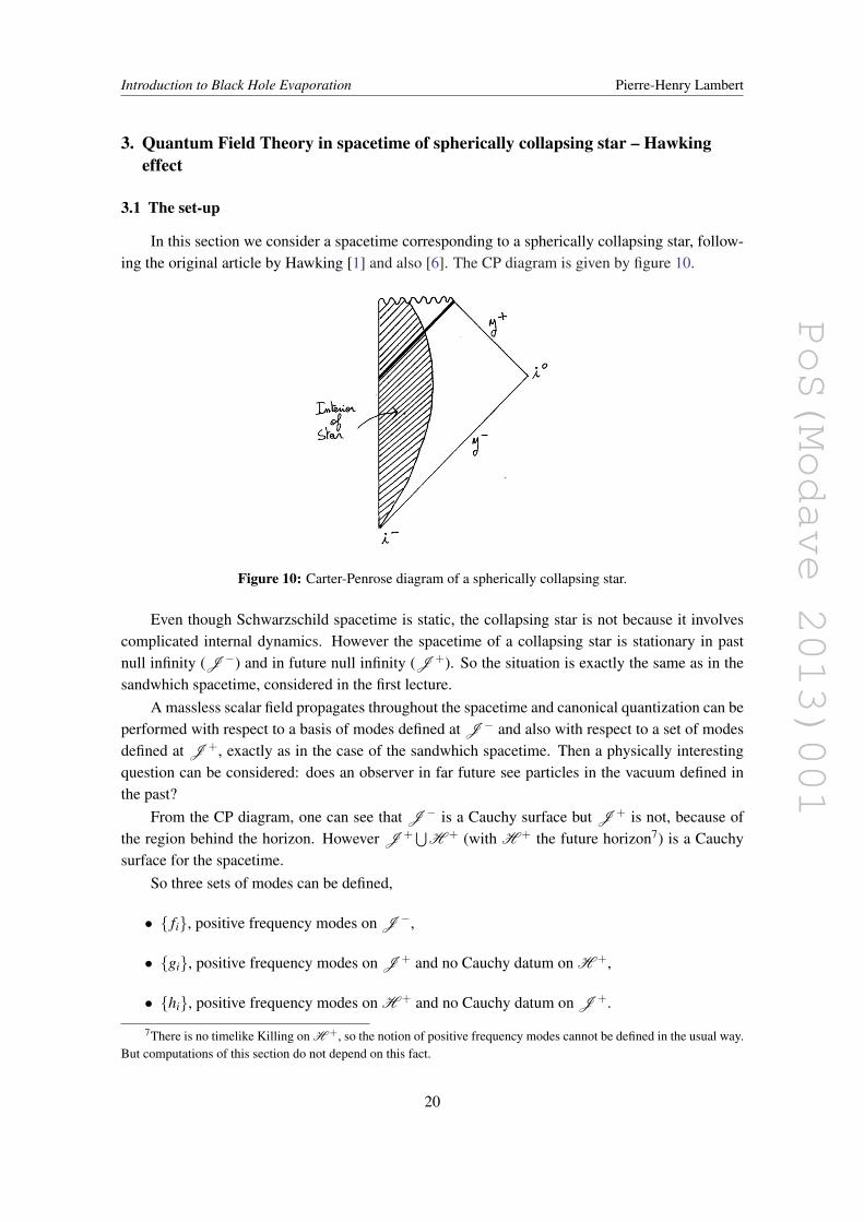
In this section we consider a spacetime corresponding to a spherically collapsing star, follow-ing the original article by Hawking [1] and also [6]. The CP diagram is given by figure 10.

Figure 10: Carter-Penrose diagram of a spherically collapsing star.

Even though Schwarzschild spacetime is static, the collapsing star is not because it involvescomplicated internal dynamics. However the spacetime of a collapsing star is stationary in pastnull infinity (J −) and in future null infinity (J +). So the situation is exactly the same as in thesandwhich spacetime, considered in the first lecture.

A massless scalar field propagates throughout the spacetime and canonical quantization can beperformed with respect to a basis of modes defined at J − and also with respect to a set of modesdefined at J +, exactly as in the case of the sandwhich spacetime. Then a physically interestingquestion can be considered: does an observer in far future see particles in the vacuum defined inthe past?

From the CP diagram, one can see that J − is a Cauchy surface but J + is not, because ofthe region behind the horizon. However J +⋃H + (with H + the future horizon7) is a Cauchysurface for the spacetime.

So three sets of modes can be defined,

• fi, positive frequency modes on J −,

• gi, positive frequency modes on J + and no Cauchy datum on H +,

• hi, positive frequency modes on H + and no Cauchy datum on J +.

7There is no timelike Killing on H +, so the notion of positive frequency modes cannot be defined in the usual way.But computations of this section do not depend on this fact.

20

PoS(Modave 2013)001


Modes fi, f ∗i form a complete set, and gi,g∗i ⋃hi,h∗i , when taken together also form a com-

plete set.The next stage is to expand any field configuration φ solution to the equation of motion in

terms of the two different complete sets of modes,

φ = ∑i(ai fi +h.c.) = ∑

i(bigi + cihi +h.c.). (3.1)

The vacuum with respect to the basis fi, f ∗i is defined to be the state |in〉 such that ai|in〉= 0,∀i,and the number of particles seen by an observer in far future in the |in〉 vacuum is given by Ni =

(BB†)ii. The Bogoliubov coefficient of the expansion gi =∑ j(Ai j f j+Bi j f ∗j ) is thus needed in orderto compute the particles number we are looking for. A natural way of computing this Bogoliubovcoefficient is first to find a solution to the equation of motion in the Schwarzschild background andthen to go to Fourier space doing the same analysis as in the case of the Rindler space.

The problem of this straightforward approach is that there is no easy solution of the equationof motion in the Schwarzschild background, as will be seen in the next section.

3.2 Wave equation

The schwarzschild metric is

ds2 =−(

1− 2Mr

)dt2 +

(1− 2M

r

)−1

dr2 + r2dΩ2, (3.2)

with dΩ2 = dθ 2 + sin2θdφ 2. We have

√−g = r2 sinθ and the wave equation ϕ = 0 read

ϕ =1√−g

∂µ

(gµν√−g∂νϕ

),

= ∂t

(−(

1− 2Mr

)−1

∂tϕ

)+

1r2 ∂r

((1− 2M

r

)r2

∂rϕ

)+

1r2S2ϕ, (3.3)

with S2ϕ =(

1sinθ

∂θ (sinθ∂θ )+1

sin2θ

∂ 2φ

)ϕ . The ansatz ϕ = f (r,t)

r Y ml (θ ,φ) reduces the wave equa-

tion (3.3) to

−(

1− 2Mr

)−1

∂2t f +

2Mr2

(∂r f − 1

rf)+

(1− 2M

r

)∂

2r f − l(l +1)

r2 f = 0. (3.4)

The last term comes from the property of the spherical harmonics, S2Y ml = −l(l + 1)Y m

l . Let usintroduce the tortoise coordinate r∗ by

dr∗ =dr

1− 2Mr

(3.5)

∂r =∂r∗

∂r∂r∗ =

(1− 2M

r

)−1

∂r∗

∂2r =−

(1− 2M

r

)−2 2Mr2 ∂r∗+

(1− 2M

r

)−2

∂2r∗ .

21

PoS(Modave 2013)001


In terms of the tortoise coordinate the wave equation (3.4) takes the form

(−∂2t +∂

2r∗) f −

(1− 2M

r

)(l(l +1)

r2 +2Mr3

)f = 0. (3.6)

Let us call the potential V =(1− 2M

r

)( l(l+1)r2 + 2M

r3

). Then the wave equation becomes

(−∂2t +∂

2r∗) f =V f . (3.7)

The tortoise coordinate r∗ defined by (3.5) is given explicitly in terms of the coordinate r by

r∗ =∫

drr−2M+2M

r−2M= r+2M ln(r−2M)+C = r+2M ln

( r2M−1),

where the integration constant C was chosen to be C = −2M ln(2M). The name tortoise comesfrom the derivative

drdr∗

= 1− 2Mr

, limr→2M

drdr∗

= 0,

which means that the function r = r(r∗) becomes more and more constant as one approaches thehorizon, hence the name.

Let us look at the form of the potential V ,

• r→ 2M (⇔ r∗ =−∞) : V = 0,

• r→ ∞ (⇔ r∗ =+∞) : V = 0,

and between these two values of r, the precise form of the potential V depends on l, and representsa potential barrier, so that any solution coming from infinity is expected to be partially reflectedand partially emitted. At J + the potential is zero and the wave equation reduces to

(−∂2t +∂

2r∗) f = 0, (3.8)

solutions of which are plane waves8.Later on outgoing plane wave solution to (3.8) will be considered,

f = eikµ xµ

, kµ = (−ω,k),xµ = (t,r∗)

= e−iωu (3.9)

Now an approximation9 is made, the geometric optics approximation.

8Note that plane waves are delocalized (i.e. they have a support everywhere on J +) but wave packets (i.e. a linearcombination of planes waves) can be constructed on J + around some momentum ω0 [6] by using the superpositionprinciple .

9Cfr. the original paper by Hawking [1].

22

PoS(Modave 2013)001


3.3 Geometric optics approximation

A general wave f given by f = aeiS is such that a is constant with respect to the phase S, thisis the geometric optics approximation [16]. The wave equation f = 0 implies

0 = DµDµ(aeiS) = Dµ(i(DµS) f ) = i(DµDµS) f − (DµS)(DµS) f

= iSDµDµ f − (DµS)(DµS) f , (3.10)

where double integration by parts were done to get the first term of (3.10). But then equation ofmotion f = 0 implies that (3.10) reduces to

DµSDµS = 0. (3.11)

Suppose moreover that S(x) is a family of surfaces of constant phase. The normal vector to S(x) iskµ = ∂µS and condition (3.11) is equivalent to the condition that the normal vector is null,

kµkµ = 0. (3.12)

Due to its light-like nature, the vector kµ is also normal to some tangent vector kµ for a certaincurve xµ(λ ) lying in the surface S(x), i.e. kµ = dxµ

dλ.

A special property of kµ is that it is the tangent vector of a very specific class of curves, namelykµ is the tangent vector field of null geodesic curves. Indeed, by taking the covariant derivative of(3.12)

0 = kµkµ ⇒ 0 = 2kµDσ kµ = 2(kµDσ (∂µS)) = 2(kµDµ(∂σ S))

0 = kµDµkσ . (3.13)

Equation (3.13) is the geodesic equation. Indeed,

0 = kµDµkσ = kµ∂µkσ + kµ

Γσµνkν =

d2xσ

dλ 2 +Γσµν

dxµ

dλ

dxν

dλ,

where the fact that kµ is the tangent vector to a certain curve was used, kµ = dxµ

dλ.

In conclusion, the geometric optics approximation implies that the surface of constant phase ofany wave f = aeiS can be traced back in time by following null geodesics. That is the approximationthat Hawking did in his original paper, and that is the approximation that is done in the next section.

3.4 Hawking’s computation

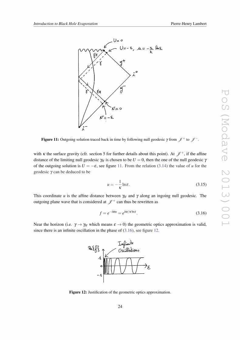
At J + an outgoing solution to the wave equation was found to be f = e−iωu, cfr. (3.9). Thegeometric optics approximation is used10 to trace back in time the outgoing solution by followingnull geodesics, see figure 11.

Let γH denote the limiting null geodesic staying at the horizon, and suppose that the nullgeodesic γ associated with the outgoing solution (3.9) is close to γH . The affine distance at J + isU (the Kruskal coordinate), and is related to u = t− r∗ by the relation

U =−e−uκ , (3.14)

10This approximation will be justified later.

23

PoS(Modave 2013)001


Figure 11: Outgoing solution traced back in time by following null geodesic γ from J + to J −.

with κ the surface gravity (cfr. section 5 for further details about this point). At J +, if the affinedistance of the limiting null geodesic γH is chosen to be U = 0, then the one of the null geodesic γ

of the outgoing solution is U = −ε , see figure 11. From the relation (3.14) the value of u for thegeodesic γ can be deduced to be

u =− 1κ

lnε. (3.15)

This coordinate u is the affine distance between γH and γ along an ingoing null geodesic. Theoutgoing plane wave that is considered at J + can thus be rewritten as

f = e−iωu = eiω/κ lnε . (3.16)

Near the horizon (i.e. γ → γH which means ε → 0) the geometric optics approximation is valid,since there is an infinite oscillation in the phase of (3.16), see figure 12.

Figure 12: Justification of the geometric optics approximation.

24

PoS(Modave 2013)001


According to the geometric optics approximation, surfaces of constant phase of the solution(3.16) can be traced back in time by following the null geodesic γ . When tracing back in time, γ

will reach J − at an affine distance v =−ε with respect to the limiting null geodesic γH . So

• at J +, the outgoing solution is f = eiω/κ lnε ,

• at J −, the outgoing solution is f = eiω/κ ln−v.

This solution at J − has exactly the same form as the one for the Rindler space case, but now withκ instead of a. The same business as for Rindler space can be done, i.e. going into Fourier space,comparing with Bogoliubov expansion and using funny integrals to conclude that the number ofparticles is given by

|B|2 = 1e2πω/κ −1

, T = κ/2π. (3.17)

This is a Planck spectrum with temperature T = κ/2π; this is the Hawking radiation: a black holehas a temperature and his thermal emission leads to a decrease in the mass of the black hole andpossibly to its evaporation.

An important remark is that during this presentation, the potential barrier of the potential V wasnot taken into account. This is the backreaction problem and when it is considered the spectrum ismodified in the following way

|B|2 = 1e2πω/κ −1

Γω , (3.18)

where Γω is the greybody factor, depending on the spin and angular part of the potential V . Theimportant point to observe here in this case is that the spectrum is no longer thermal when thebackraction is taken into account. On the other side, if the backreaction problem is not consideredthen the precise form of the potential V in −∂ 2

t + ∂ 2r∗ f = V f is totally irrelevant in the geometric

optics approximationIn the next section some consequences of Hawking radiation are studied.

25

PoS(Modave 2013)001


4. Some consequences of Hawking radiation

4.1 Thermodynamics of black holes

Before Hawking discovered that black holes radiates at temperature T = κ/2π there was ananalogy between the laws of thermodynamics and the laws of black holes. Then Hawking provedthat black holes are actually thermal objects, so the initial analogy is more than just an analogy.

The zeroth law of thermodynamics states that the temperature T of a body in thermal equilib-rium is constant. One can wonder what is the analogous for the black hole but of course from theresult presented in the previous section, the answer is already known. In this section κ is shown tobe constant on the black hole horizon.

4.1.1 Surface gravity

In this part, let us consider [5] an hypersurface S(x), the normal of which is lµ = gµν∂νS andis null, lµ lµ = 0. From (3.13) it is already known that lµ is the tangent vector field to null geodesicscurves.

DEFINITION 7A null hypersurface Σ is called Killing horizon of a Killing vector field ξ if the Killing vector fieldξ is proportional to l, namely ξ µ = f lµ , for some smooth function f .

Let us compute ξ µDµξ σ , remembering the geodesic equation (3.13),

ξµDµξ

σ = ( f lµ)(Dµ f )lσ +( f lµ) f Dµ lσ = ( f lµ)(∂µ f )lσ = (ξ µ∂µ ln f )ξ σ . (4.1)

The surface gravity κ is defined by κ = ξ µ∂µ ln f , then (4.1) becomes

ξ µDµξ σ = κξ σ . (4.2)

This relation allows to compute the surface gravity more easily than using his definition. Forinstance, for the Schwarzschild black hole in ingoing Eddington-Finkelstein coordinates11, themetric reads

ds2 =−(

1− 2Mr

)dv2 +2dvdr+ r2dΩ

2,

with ∂v a (timelike) Killing vector, K = Kµ∂µ with Kµ = (1,0,0,0). The computation of (4.2) withσ = v gives an expression for the surface gravity,

ξσ Dσ ξ

v = ξσ

∂σ ξv +ξ

σΓ

vσκξ

κ = Γvvv =−

12

gvrgvv,r =Mr2 .

This result should be evaluated at the horizon, by taking r = 2M, and so the surface gravity for theSchwarzschild black hole is given by

κ = 14M . (4.3)

11The computation is easier in this coordinates system.

26

PoS(Modave 2013)001


4.1.2 Some properties of κ

One can wonder why κ is called the surface gravity, this is the purpose of this sub-section. Inorder to do this, the fact that κ is constant on the horizon is required, for which two other propertiesof κ are needed.

1. First, the Killing vector of a Killing horizon is by definition orthogonal to a hypersurface.Frobenius theorem can then be used to say that

ξ[µDνξσ ] = 0, (4.4)

where brackets denote antisymmetrization. The fact that ξ is a Killing vector, hence Dµξν +

Dνξµ = 0, reduces relation (4.4) to

0 = ξµDνξσ +ξνDσ ξµ +ξσ Dµξν = ξµDνξσ −ξνDµξσ +ξσ Dµξν ,

ξσ (Dµξν) =−(ξµDνξσ −ξνDµξσ ). (4.5)

Contracting equation (4.5) with (Dµξ ν) yields

(Dµξ

ν)ξσ (Dµξν) =−2(Dµξ

ν)(ξµDνξσ ),

=−2κξνDνξσ ,

=−2κ2ξσ , (4.6)

where (4.2) was used. The first property of κ is obtained,

κ2 =−12(D

µξ ν)(Dµξν) . (4.7)

2. To prove the second property of κ , the definition of the Riemann tensor is used, i.e. thecommutator of two covariant derivative acting on a vector field,

[Dµ ,Dν ]vσ = R κ

µνσ vκ , ∀vσ . (4.8)

If the vector field is a Killing vector, i.e. vσ = ξσ , then (4.8) becomes

DµDνξσ +DνDσ ξµ = R κ

µνσ ξκ . (4.9)

Writing (4.9) three times by permuting the indices yields the relation

2DµDνξσ = (R κ

µνσ −R κ

νσ µ +R κ

σ µν )ξκ . (4.10)

Finally the Bianchi identity R κ

[µνσ ] = 0 allows to write

R κ

µνσ +R κ

σ µν =−R κ

νσ µ ,

and this relation simplifies (4.10) to DµDνξσ =−R κ

νσ µ ξκ . Equivalently,

DµDνξσ = R κ

σνµ ξκ . (4.11)

27

PoS(Modave 2013)001


3. The first two properties are needed to prove that the surface gravity κ is constant on thehorizon, or more precisely on the orbits of the vector field ξ [5].

The proof goes as follow. Let us consider t, a tangent vector field to some null hypersurfaceN . From the first property (4.7), we have

tσ Dσ κ2 =−(Dµ

ξν)tσ Dσ (Dµξν). (4.12)

By hypothesis ξ is a null Killing vector, so it is both normal and tangent to the hypersurfaceN , so tσ can be chosen as tσ = ξ σ and equation (4.12) reduces to

ξσ Dσ κ

2 =−(Dµξ

ν)ξ σ Dσ Dµξν =−(Dµξ

ν)ξ σ Rµνσκξκ = 0. (4.13)

Where the second property (4.11) was used and also the fact that the sum over indices σ ,κ

that are symmetric in the ξ ’s while antisymmetric in the Riemann is zero. The surface gravityis thus constant on the orbits of ξ . This is the zeroth law of black holes dynamics.

4. To explain the name of κ , let us consider a particle on a timelike orbit of a Killing field ξ .The worldline of the particle is xµ = xµ(λ ). Because the particle is moving along an orbit ofa Killing field, the four-velocity uµ is proportional to ξ µ and the factor of proportionality isfixed by requiring the normalization u2 = uµuµ =−1,

uµ = Aξµ ⇒ u2 =−1 = A2

ξµ

ξνgµν ⇒ A2 =

−1ξ 2 .

The four-velocity is thus given by uµ = ξ µ√−ξ 2

. The four-acceleration of the particle along

the orbit is

aµ =Duµ

dλ= uσ Dσ uµ =

ξ σ√−ξ 2

Dσ

ξ µ√−ξ 2

,

but ξ σ Dσ ξ 2 = 2ξ σ ξ νDσ ξν = 0, because of the antisymmetry of the indices in the two lastfactors, and the symmetry of them in the to first factors so that the total sum is zero. Theacceleration is thus given by

aµ = ξ σ Dσ ξ µ

−ξ 2 . (4.14)

On the horizon −ξ 2 is nothing else but the square of the red-shift factor. For instance in thecase of the Schwarzschild black hole in ingoing Eddigton-Finkelstein coordinates,

ds2 =−(

1− 2Mr

)dv2 +2dvdr+ r2dΩ

2, (4.15)

∂v is a (timelike) Killing vector and we have −ξ 2 =−gvv =(1− 2M

r

).

The relation (4.2) allows to rewrite the acceleration (4.14) as aµ = κξ µ

−ξ 2 , so we have

κ = limH Va , (4.16)

with V =√−ξ 2,a =

√−aµaµ . This result means that κ is the limiting acceleration when

the particle approaches the horizon, hence the name of surface gravity.

28

PoS(Modave 2013)001


5. Finally, the relation (3.15) between the affine distance and the surface gravity is established asfollow. Consider the Killing vector ξ of a Killing horizon, ξ = ∂

∂αfor some curve α = α(λ )

with affine parameter λ . Thus,

ξ = ∂λ

∂α

∂

∂λ≡ f l with f = ∂λ

∂α, l = ∂

∂λ.

The surface gravity is defined by κ = ∂ ln f∂α

and is constant on the horizon. From the definitionwe get ln f = κα + lnκ where the integration constant is chosen to be lnκ , so that f = κeκα .But f is defined by f = ∂λ

∂α, hence the relation between the affine distance λ and the surface

gravity κ is

λ = eκα . (4.17)

In (3.15) the affine parameter was defined to be λ = ε and moreover α =−u.

4.1.3 The laws

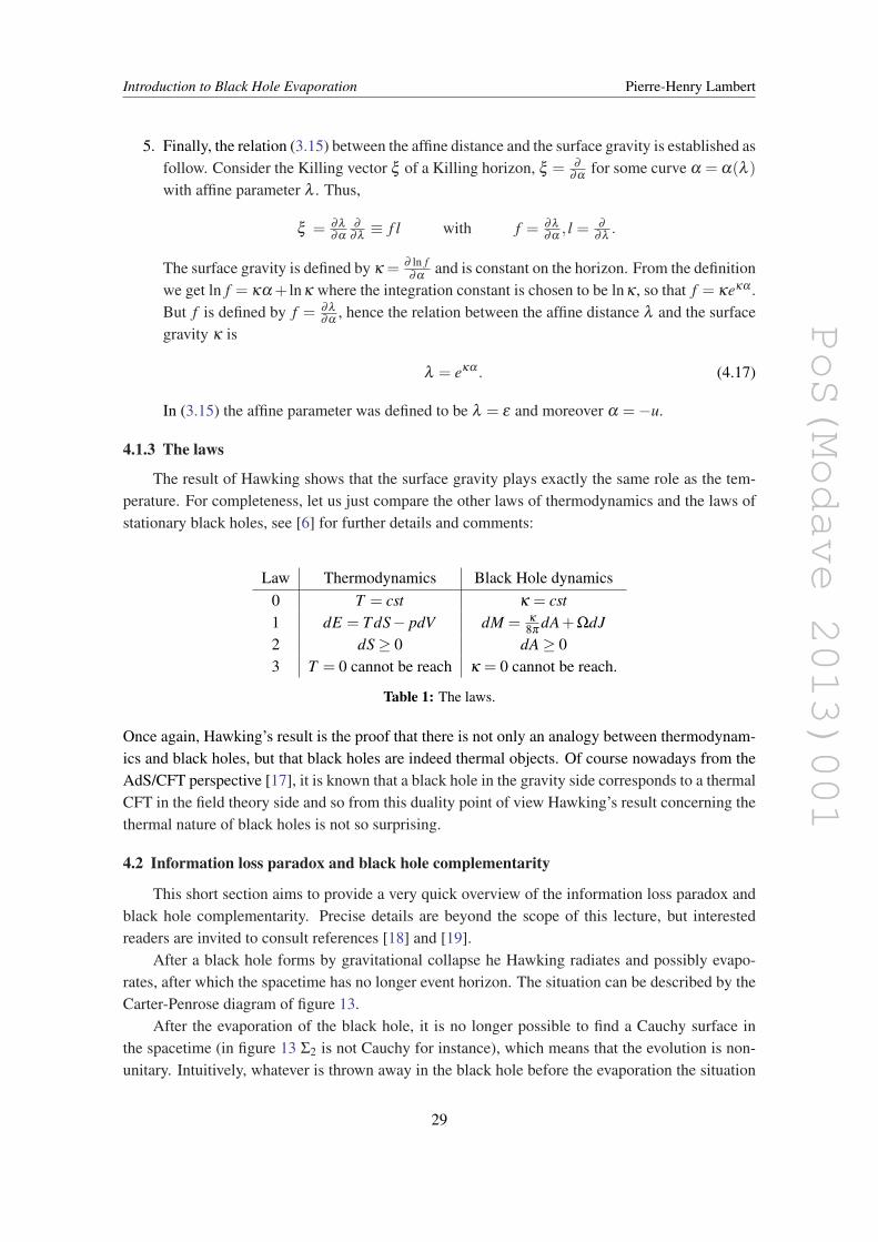
The result of Hawking shows that the surface gravity plays exactly the same role as the tem-perature. For completeness, let us just compare the other laws of thermodynamics and the laws ofstationary black holes, see [6] for further details and comments:

Law Thermodynamics Black Hole dynamics0 T = cst κ = cst1 dE = T dS− pdV dM = κ

8πdA+ΩdJ

2 dS≥ 0 dA≥ 03 T = 0 cannot be reach κ = 0 cannot be reach.

Table 1: The laws.

Once again, Hawking’s result is the proof that there is not only an analogy between thermodynam-ics and black holes, but that black holes are indeed thermal objects. Of course nowadays from theAdS/CFT perspective [17], it is known that a black hole in the gravity side corresponds to a thermalCFT in the field theory side and so from this duality point of view Hawking’s result concerning thethermal nature of black holes is not so surprising.

4.2 Information loss paradox and black hole complementarity

This short section aims to provide a very quick overview of the information loss paradox andblack hole complementarity. Precise details are beyond the scope of this lecture, but interestedreaders are invited to consult references [18] and [19].

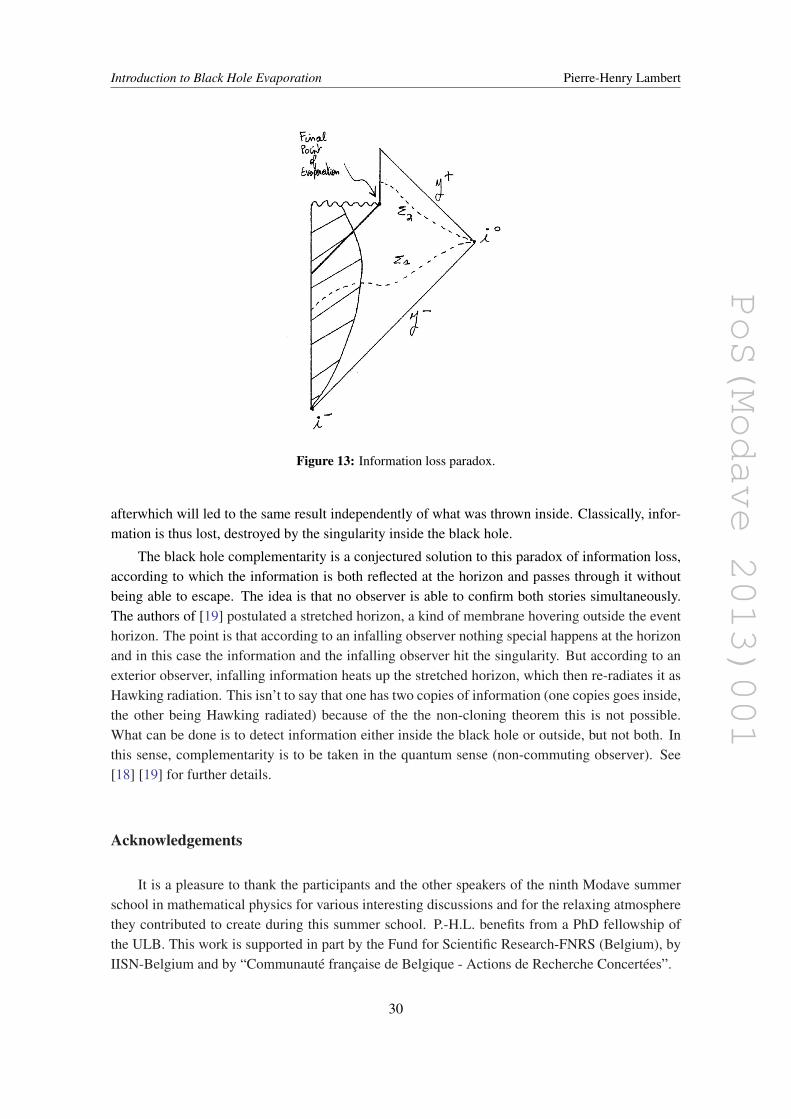
After a black hole forms by gravitational collapse he Hawking radiates and possibly evapo-rates, after which the spacetime has no longer event horizon. The situation can be described by theCarter-Penrose diagram of figure 13.

After the evaporation of the black hole, it is no longer possible to find a Cauchy surface inthe spacetime (in figure 13 Σ2 is not Cauchy for instance), which means that the evolution is non-unitary. Intuitively, whatever is thrown away in the black hole before the evaporation the situation

29

PoS(Modave 2013)001


Figure 13: Information loss paradox.

afterwhich will led to the same result independently of what was thrown inside. Classically, infor-mation is thus lost, destroyed by the singularity inside the black hole.

The black hole complementarity is a conjectured solution to this paradox of information loss,according to which the information is both reflected at the horizon and passes through it withoutbeing able to escape. The idea is that no observer is able to confirm both stories simultaneously.The authors of [19] postulated a stretched horizon, a kind of membrane hovering outside the eventhorizon. The point is that according to an infalling observer nothing special happens at the horizonand in this case the information and the infalling observer hit the singularity. But according to anexterior observer, infalling information heats up the stretched horizon, which then re-radiates it asHawking radiation. This isn’t to say that one has two copies of information (one copies goes inside,the other being Hawking radiated) because of the the non-cloning theorem this is not possible.What can be done is to detect information either inside the black hole or outside, but not both. Inthis sense, complementarity is to be taken in the quantum sense (non-commuting observer). See[18] [19] for further details.

Acknowledgements

It is a pleasure to thank the participants and the other speakers of the ninth Modave summerschool in mathematical physics for various interesting discussions and for the relaxing atmospherethey contributed to create during this summer school. P.-H.L. benefits from a PhD fellowship ofthe ULB. This work is supported in part by the Fund for Scientific Research-FNRS (Belgium), byIISN-Belgium and by “Communauté française de Belgique - Actions de Recherche Concertées”.

30

PoS(Modave 2013)001


References

[1] S. Hawking, Particle Creation by Black Hole, Commun. Math. Phys. 43, 199-220 (1975).

[2] N. Birrell, P. Davies, Quantum fields in curved space, Cambridge University Press, Cambridge (1984)

[3] R. Wald, Quantum Field Theory in Curved Spacetime and Black Hole Thermodynamics, TheUniversity of Chicago Press, Chicago (1994).

[4] S. Carroll, Spacetime and Geometry: An Introduction to General Relativity, Addison Wesley (2004).

[5] P. Townsend, Black Holes, Preprint gr-qc/9707012.

[6] F. Dowker, Black Holes, Lectures notes, Imperial College London, available athttps://dl.dropboxusercontent.com/u/9717190/bh.pdf.

[7] M. Henneaux, Relativité Générale, Lectures notes, Université Libre de Bruxelles, unpublished.

[8] S. Hawking and G. Ellis, The large scale structure of space-time, Cambridge University Press,Cambridge (1973).

[9] S. Avis, C. Isham and D. Storey, Quantum field theory in anti-de Sitter space-time, Phys. Rev D 18,3565-3576 (1978).

[10] R. Geroch, Domain of dependence, J. Math. Phys 11, 437-449 (1970).

[11] C. Kiefer, Thermodynamics of black holes and Hawking radiation, in Classical and Quantum BlackHoles, IOP (2002).

[12] A. Wipf, Quantum fields near Black Holes, in Black Holes: Theory and Observation, lectures notes inPhysics 514, 385-415 (1998), Preprint hep-th 9801025.

[13] V. Mukhanov and S. Winitzki, Introduction to Quantum Effects in Gravity, Cambridge UniversityPress, Cambridge (2007).

[14] J. Traschen, An Introduction to Black Hole Evaporation, Preprint qc/0010055.

[15] G. Barnich, Théorie quantique des champs, Lectures notes, Université Libre de Bruxelles, available athttp://homepages.ulb.ac.be/~gbarnich/TQC.pdf.

[16] L. Landau and E. Lifshitz, The Classical Theory of Field, Butterworth Heinemann.

[17] O. Aharony, S. S. Gubser, J. Maldacena, H. Ooguri, and Y. Oz, Large N field theories, string theoryand gravity, Phys. Rept. 323 (2000) 183–386, Preprint hep-th/9905111.

[18] S. Hawking, Breakdown of predicability in gravitational collapse, Phys. Rev. D 14, 2460-2473(1976).

[19] L. Susskind, L. Thorlacius and J. Uglum, The stretched horizon and black hole complementarity,Phys. Rev D 48, 3743-3761 (1993).

31

http://arxiv.org/abs/gr-qc/9707012

http://arxiv.org/abs/hep-th/9801025

http://arxiv.org/abs/gr-qc/0010055

http://arXiv.org/abs/hep-th/9905111

Documents

Introduction to Black Hole Evaporation