The importance of the financial system for the real economy

Empir Econ (2017) 53:1553–1586DOI 10.1007/s00181-016-1175-4

The importance of the financial system for the realeconomy

Sebastian Ankargren1 · Mårten Bjellerup2 ·Hovick Shahnazarian3

Received: 19 February 2015 / Accepted: 12 August 2016 / Published online: 27 September 2016© The Author(s) 2016. This article is published with open access at Springerlink.com

Abstract This paper first describes financial variables that have been constructedto correspond to various channels in the transmission mechanism. Next, a BayesianVARmodel for the macroeconomy, with priors on the steady states, is augmented withthese financial variables and estimated using Swedish data for 1989–2015. The resultssupport three conclusions. First, the financial system is important and the strength ofthe results is dependent on identification, with the financial variables accounting for10–25% of the forecast error variance of Swedish GDP growth. Second, the suggestedmodel produces an earlier signal regarding the probability of recession, compared to amodel without financial variables. Third, the model’s forecasts for the deep downturnin 2008 and 2009, conditional on the development of the financial variables, outper-form a macro-model that lacks financial variables. Furthermore, this improvementin modelling Swedish GDP growth during the financial crisis does not come at theexpense of unconditional predictive power. Taken together, the results suggest thatthe proposed model presents an accessible possibility to analyse the macro-financiallinkages and the GDP developments, especially during a financial crisis.

Keywords Transmission channels · Financial indicators · Macroeconomy · Businesscycle · Credit cycle · Bayesian VAR

JEL Classification E37 · E44

B Sebastian [email protected]

1 Department of Statistics, Uppsala University, Box 513, 751 20 Uppsala, Sweden

2 Swedish National Debt Office, 103 74 Stockholm, Sweden

3 Ministry of Finance, 103 33 Stockholm, Sweden

123

http://crossmark.crossref.org/dialog/?doi=10.1007/s00181-016-1175-4&domain=pdf

1554 S. Ankargren et al.

1 Introduction

In late 2008, during the peak of the financial crisis, several markets at the heart of thefinancial system more or less stopped functioning. Liquidity in the interbank marketdried up as banks refrained from lending money, even at short maturities. The price ofmany assets fell quickly and deeply, central banks cut their policy rates drastically, andthe situation was characterized by great uncertainty. The crisis deepened the incipientrecession sharply, and most economists and policy makers were, at the time, surprisedby the dramatic effects on the real economy. But the close link between the financialsystem and the real economy is not only there in times of crisis; it is also in placeunder more normal economic circumstances. The effects are just less drastic.

In the wake of the financial crisis, researchers and policy makers have directedmuchmore attention to the linkage between the financial system and the real economy,known as the transmissionmechanism.1 Great theoretical and empirical effort has beendevoted to better understand the way financial shocks affect the real economy (see,for example, Bloom 2009; Bloom et al. 2012; Christiano et al. 2014). An importantpart of the increased attention is that several governments are now considering morefar-reaching changes in supervisory and regulatory structures in order to protect thereal economy from the recurrent malfunctioning of the financial sector.2

However, if regulation is to be successful, at least two conditions have to be fulfilled.First, policy makers need to have a qualitative knowledge of how the financial marketsaffect the real economy through the transmission mechanism. Second, policy makersneed to have quantitative knowledge of the transmission mechanism in order to makea balanced choice of the magnitude of a specific regulative measure.

Early efforts on modelling the transmission mechanism have largely focused onmodelling individual channels within the transmission mechanism, while later efforts,not least within the dynamic stochastic general equilibrium (DSGE) literature, havea richer modelling of the transmission mechanism.3 It should be pointed out thatthere are many studies that examine what effect individual transmission channels haveon the real economy. There are to our knowledge no empirical papers that estimatethe impact of all transmission channels.4 The idea of this paper is to fill this gap bysuggesting a description of the transmission mechanism that fits into a small-scaleBayesian VAR (BVAR) model. Despite being limited in terms of variables, the modeloffers a number of possibilities in analysing various developments in financialmarkets.The reason is that the financial variables used in the model are composites of severalfinancial variables, which in turn stem from the detailed underlying description of thetransmission mechanism. BVAR models resembling the one used in this paper have

1 See, for instance, Basel Committee (2011).2 See, for instance, Basel Committee (2012a).3 See the survey from Basel Committee (2012b) and Brunnermeier et al. (2012). Jermann and Quadrini(2012) and Christiano et al. (2014) are examples of two structural DSGE models that include financialfrictions in their models.4 However, there are general equilibrium models with a much more detailed modelling of the economythat take account of several transmission channels at the same time. See, for example, Brunnermeier et al.(2012).

123

The importance of the financial system for the real economy 1555

been successfully used in related applied work (see, for example, Österholm 2010;Jarocinski and Smets 2008 among others).

The model is essentially used to answer two questions: (i) Is the financial systemimportant for the development in the real economy? (ii) If it is, what are the charac-teristics?

The paper has the following structure. In Sect. 2, we construct four compositefinancial variables that act as indicators for the transmissions channels using datafrom Sweden. In Sect. 3, the details of the statistical model of our choice, a BVARmodel with a prior on the steady state, are given. In Sect. 4, the model is used to answerthe two questions we have posed. Moreover, Sect. 4 investigates the robustness of theresults by conducting a sensitivity analysis. Section 5 concludes.

2 Choice and construction of the financial variables

The financial system mainly affects the real economy through the following transmis-sion channels: the balance sheet channel, the interest rate channel, the bank capitalchannel and the uncertainty channel. “Appendix” describes negative external effectsthat cause the accumulation and liquidation of financial imbalances and the way theidentified negative externalities affect the real economy through the different trans-mission channels. The purpose of this section is to describe the variables that weuse to quantify and isolate the impact of different transmissions channels on the realeconomy.

2.1 Asset price gap and credit gap: the balance sheet channel

The balance sheet channel describes how falling asset prices affect households andfirms’ balance sheet, solvency and creditworthiness, and the impact that this may haveon consumption and investment. The prices of financial and real assets are importantfor the solvency of firms and households. In order to capture the variations in bothfinancial and real asset prices, a summary index is therefore created based on howthe share and property prices change in relation to their historical trends. A gap isgenerated for each of the stock and property markets as a first step towards creatinga summary variable. The stock price gap and the house price gap are defined as thedeviation of the stock market index and the property price index from their trenddivided by the trend.5 In the second step, the share price gap (20%) and the propertyprice gap (80%) are combined in an asset price gap that summarizes the developmentof house and stock prices.6

5 The trend is calculated through a one-sided HP filter using a value of the weighting parameter equal to400 000 (see, for example, Drehmann et al. 2010). The Basel Committee suggests using this method tocalculate the credit gap which is the deviation of the credit-to-GDP ratio from its long-term trend. The studyby Drehmann et al. (2010) indicates that the credit gap has been useful in signalling financial crises in thepast.6 Although the weighting is subjective, the aim has been to find weights that create a clear linkage betweenthe wealth gap and the GDP growth. The size of the weights also corresponds to the relative size of thevariance of the share price and property price gaps. We have also estimated the model with individual series

123


Economic shocks lead to a fall in the value of borrowers’ assets at the same time asthe value of their loans is unchanged. In such cases, the borrowers’ balance sheets lookmuch worse than they had expected, with the result that they amortize part of theirliabilities (consolidate their balance sheets). So, asset prices and credit can reinforceeach other through the “financial accelerator effect”. To be able to control for thismechanism, we include a credit gap to the set of variables. Technically, the credit gapis constructed in the same way as the share price gap. As a first step the credit ratio isgenerated (total lending in relation to GDP at current prices). The credit gap is definedas the deviation of the credit ratio from its trend, divided by the trend.

2.2 The interest on three months treasury bills: the interest rate channel

The interest rate channel describes how the real economy is affected when the centralbank increases the repo rate. Monetary policy affects the interest on three monthstreasury bills by changing the repo rate which is equivalent to changing the so-calledovernight rate.7

Monetary policy also affects the value of the currency (exchange rate channel).Normally, an increase in the repo rate leads to a strengthening of the krona. Astronger exchange rate—an appreciation—makes foreign goods cheaper comparedwith domestically produced goods which lead to a rise in imports, a decline in exportsand a dampening of inflationary pressure. Moreover, a stronger krona tends to lowerthe inflation rate, since imported goods and import-competing goods become cheaper.This reinforces the dampening effect on inflation of falling demand. To be able tocontrol for exchange rate channel, we also include the real exchange rate.

2.3 The lending rate: the bank capital channel

The bank capital channel describes the impact that various risks have on bank balancesheets and income statements and ultimately on their pricing behaviour and lending.As in Karlsson et al. (2009), it is assumed that banks in Sweden operate on a marketcharacterized by monopolistic competition in which the banks’ lending rate is set asa markup on their marginal costs.8 The lending rate is therefore influenced by boththe interest rate that banks themselves have to pay to borrow funds and the interestrate supplement added by banks when lending on to their customers. The study byKarlsson et al. (2009) indicates that what the macroeconomic literature calls creditspread contains many different components that are affected in one way or another by

Footnote 6 continuedfor the house price gap and the share price gap and the results indicate that the conclusions of this paperremain intact.7 A treasury bill is a short-term debt instrument issued by the Swedish National Debt Office. The maturityof these instruments is usually up to one year. Treasury bills are used to finance the government’s short-termborrowing requirement.8 For amore detailed description of themarket structure and loan pricing equation, see Arregui et al. (2013),Box 2.

123


various risks associated with bank operations. Using lending rates together with policyrates in macroeconomic models makes it possible to analyse the effects these riskshave on the real economy, besides those stemming frommonetary policy. The lendingrate that is used as an indicator is a combination of the interest rate that householdsand firms actually pay on their existing loans.9

2.4 The financial stress index: the uncertainty channel

The uncertainty channel describes how more uncertainty in financial markets leads tohigher precautionary savings and lowers consumption. The degree of uncertainty onfinancial markets is measured by a “stress index”. In line with the arguments presentedin Forss Sandahl et al. (2011) and Holmfeldt et al. (2009), an index is constructed thatis a composite of developments on fourmarkets: the stockmarket, the currencymarket,the money market and the bond market.10

2.4.1 Uncertainty in the stock and currency markets

There are several ways of measuring disturbances and uncertainty in the stock andcurrency markets. One of the most important measures is volatility. There is a group ofvolatility measures that are forward-looking since they are based on option prices (e.g.VIX in the USA). But, from a practical econometric perspective, it is a disadvantagethat long time series are not available for these volatility measures. This is why thispaper uses the actual volatility in the OMX index, measured as the standard deviationfor the OMX index for the previous 30days. Moreover, the actual volatility of the SEKexchange rate against the euro, measured as the standard deviation for the prices notedfor the previous 30 days, is used as a stress indicator for the currency market.

2.4.2 Uncertainty on the money market

In the money market, banks extend loans to one another at short maturities to manageday-to-day liquidity needs. The interest rate on this interbank market is called LIBOR(STIBOR in Sweden) and is often compared with the interest rate on treasury billswith corresponding maturities. This interest rate difference, which is called the TEDspread, is used as a stress indicator for the money market.

2.4.3 Uncertainty in the bond market

The spread in interest rates between mortgage and government bonds, which is calledthe mortgage spread, says something about how sellers assess the risks associatedwith each bond. This makes this spread a good indicator of developments on these

9 The lending rate is the weighted average of the interest rates for households (2/3) and the interest rate forfirms (1/3).10 Johansson (2013) develop a more complex financial stress index and compare the development of thisnew financial stress index with a simpler. See also Österholm (2010).

123


two markets. The mortgage spread is therefore used as a stress indicator for the bondmarket.

2.4.4 Financial stress index

The four indicators are first standardized so that they can be weighted to a compositefinancial stress index. The weighting is done by giving each indicator the sameweight.The resulting index is also standardized whichmeans that the summary financial stressindex has a mean of 0 and a standard deviation of 1 by construction, which facilitatesinterpretation of the index. When the series has a value of zero, it is equal to itshistorical mean and the stress level should therefore be considered normal. With thisstandardization, a value of 1 alsomeans that the level of stress is one standard deviationhigher than normal.

3 Methodology and data

In this section, we present the empirical model that we use to model the interactionbetween the financial variables described in the previous section and the macroecon-omy.

3.1 The empirical models

In a prototypical VAR model, the number of parameters is common to be large rela-tive to the number of available observations. Inevitably, this leads to large estimationuncertainty and a risk of overfitting. BVAR models, which combine the data withthe researcher’s prior beliefs, have proved to be successful tools as informative priordistributions reduce estimation uncertainty while often generating only small biases(Giannone et al. 2015). This approach is often also associated with improved fore-casting performance (see, for example, Karlsson 2013 for a review), which makes theBVAR an attractive choice and a standard tool in applied macroeconomics (Banburaet al. 2010).

The prior distribution in a Bayesian VAR model can be specified in a number ofdifferent ways. In this paper, we use the steady-state prior (Villani 2009) as we believeit offers a natural way of incorporating prior beliefs. Additionally, from a forecastingperspective it is appealing to formulate the prior on the unconditionalmean (the “steadystate”) directly, since for increasing forecast horizons the forecasts will converge tothe model’s estimate of the unconditional mean. Furthermore, the steady-state priorhas successfully been used in similar applied research in recent years, e.g. Jarocinskiand Smets (2008); Österholm (2010); Clark (2011).

The VAR model can be written on mean-adjusted form as:

Π(L)(xt − Ψ dt ) = εt , (1)

where Π(L) = (I − Π1L − · · · − ΠmLm) is a lag polynomial of order m, xt is ann × 1 vector of stationary variables, dt is a k × 1 vector of deterministic variables, Ψ

123


is an n × k coefficient matrix and εt is an n × 1 vector of multivariate normal errorterms with mean zero and covariance matrix Σ . Note that Ψ dt is the unconditionalmean of the process, meaning that priors on Ψ reflect views about the steady states ofthe variables.

The set of unknownparameters in themodel inEq. (1) isΘ = {Ψ ,Σ,Π1, . . . ,Πm},for which priorsmust be formulated. As suggested byVillani (2009), the unconditionalmeans in Ψ are assumed to be independent and normally distributed. The specifics ofthe prior distribution of Ψ in our application are discussed in more detail in Sect. 3.4.For the remaining parameters, Σ and Π1, . . . ,Πm , several different priors could inprinciple be used since xt − Ψ dt is a standard VAR given Ψ , for which a number ofalternatives exist. In this work, we follow common practice among previous studiesemploying the steady-state prior and use a non-informative prior for the error covari-

ance matrix, p(Ψ ) ∝ |Σ |− n+12 , and a Minnesota prior for the dynamic coefficients in

Π1, . . . ,Πm .The Minnesota prior (Litterman 1979) rests upon the stylized fact that many eco-

nomic variables behave approximately as random walks. Moreover, coefficients onmore distant lags as well as coefficients on variables in equations other than theirown are a priori believed to be less important than recent lags and lags of a vari-able itself. These prior beliefs are incorporated through the use of hyperparameters,which determine the degree of certainty of the beliefs. The dynamic coefficients inΠ1, . . . ,Πm are a priori assumed to be independent and normally distributed withmeans and standard deviations given by:

E[(

Π p)i, j

]=

{δi , if i = j and p = 1,

0, otherwise(2)

√V

[(Π p

)i, j

]=

⎧⎨⎩

λ1pλ3

, if i = j,λ1λ2sipλ3 s j

, otherwise(3)

Most commonly, the prior mean δi in Eq. (2) is set to δi = 1 for all i . However, ifvariable i is believed to be stationary or mean-reverting, δi may instead be set to, e.g.0 or 0.9, as noted by Banbura et al. (2010) and Karlsson (2013). Equation (3) containsthree hyperparameters: λ1 > 0 controls the overall tightness, 0 < λ2 ≤ 1 determinesthe cross-equation shrinkage in the VAR and λ3 > 0 governs the lag decay. Largervalues of λ1 will make the prior less informative by increasing the prior variances,whereas smaller values will shrink the coefficients towards the prior means. For thecross-equation tightness λ2, the upper bound means that lags of other variables in anequation are not subject to additional shrinkage compared to own lags, while smallervalues will shrink the VARmodel to a collection of AR models. Lastly, high values ofλ3 will reduce the impact of higher-order lags, as opposed to low values which pushthe model towards making no distinction between recent and distant lags. Togetherwith si , the residual standard deviation from univariate AR(4) models used to scale

123


the coefficients, these hyperparameters parametrize the entire prior distribution for thedynamic coefficients.

There are many alternative prior distributions that may be used and for surveys ofsome of thesewe refer the reader toKarlsson (2013); Koop andKorobilis (2010).Morerecently, advances have also been made on important topics such as variable selec-tion and large BVARs. George et al. (2008) developed a stochastic search to selectingrestrictions in the BVAR, and Korobilis (2013) proposed an automatic variable selec-tion approach, which Louzis (2015) subsequently applied in conjunction with thesteady-state prior. For models of larger dimension, Banbura et al. (2010) showed thata standard BVAR with a Minnesota-style prior performs well if the overall tightnesshyperparameter λ1 is set in relation to model size.

The hyperparameters parametrizing the Minnesota prior are set in accordance withthe literature. Previous studies (e.g. Adolfson et al. 2007; Villani 2009; Österholm2010) have used an overall tightness of λ1 = 0.2, a cross-equation tightness of λ2 =0.5 and a lag decay parameter of λ3 = 1.11 As discussed by Villani (2009), therandom walk prior of δi = 1 for all i is not consistent with the notion of a steady state.Instead we set δi = 0.9 for variables in levels and δi = 0 for differenced or growthvariables. We investigate the sensitivity of the hyperparameters and the prior for Ψ inthe sensitivity analysis in Sect. 4.5.

3.2 Data

Specification of the model is subject to a trade-off between including all possiblevariables and, on the other hand, parsimony. Since the degrees of freedom are quicklyexhausted when the number of variables and lags increases, a relatively small numberof variables is advisable. Too few variables and lags, however, will create problemswith omitted variable bias.

Our approach is to start with a small VAR model containing the most importantmacroeconomic variables. This type ofmodel is often used to analyse different types ofshocks (see, for example, Sims 1992; Gerlach and Smets 1995 for early contributions).The original models typically included three variables: a short-term interest rate, theinflation rate and GDP growth. This paper expands on the three-variable model byalso including unemployment so as to be able to take account of developments on thelabour market. Since Sweden is a small, open economy, the currency rate and foreignGDP growth are also included in the set of variables.12 Inflation is calculated basedon the core consumer price index (CPIX), which is CPI with households’ mortgagecosts and direct effects of indirect taxes excluded. Foreign GDP growth is calculatedas a KIX13 weighted GDP growth using the 16 most important countries for Sweden.

11 Despite the chosen values being standard choices, they are nonetheless arbitrary. An alternative is ahierarchical approach, which is discussed in detail by Giannone et al. (2015). By integrating out the modelparameters,we canobtain the likelihoodof the data given the hyperparameters, called themarginal likelihood(ML). Maximization of the ML as a function of the hyperparameters is an empirical Bayes strategy withgood performance, as demonstrated by the authors.12 The exchange rate is also included to handle the exchange rate channel.13 KIX is a weighted effective exchange rate index calculated by the Riksbank.

123


Table 1 Variables and steady-state priors

Short name Series Macro-model Financial model Steady-state prior intervalsa

1992Q4 and earlier 1993Q1 and later

GDPF KIXb weightedforeign realGDP growth

x x (0, 1) (0.25, 0.75)

SI Financial stressindex

x (−3, 3) (−1, 1)

GDP Swedish realGDP growth

x x (0.25, 0.875) (0.5, 0.625)

CPIX Core consumerprice indexinflation

x x (0.375, 0.9375) (0.25, 0.5625)

U Unemploymentrate

x x (4, 6) (5.7, 6.7)

ITB Interest on threemonthtreasury bills

x x (5.5, 8) (3, 4.5)

IL Lending rate x (6.5, 9) (4, 5.5)

AGAP Asset price gap x (−4, 4) (−2, 2)

CGAP Credit gap x (−4, 4) (−2, 2)

ER KIXb (firstdifference)

x x (−3.1, 3.1) (−3, 3)

a The steady-state priors are presented as 95% prior probability intervals for the unconditional means. Theunderlying distributions are independent normalsb KIX is a weighted effective exchange rate index calculated by the Riksbank

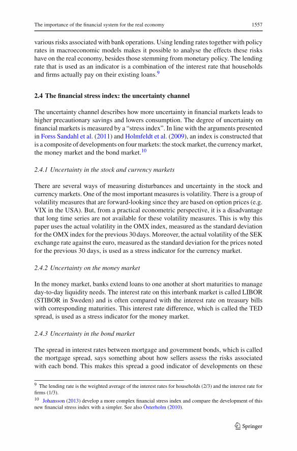
In a second step, we augment the six-variable macroeconomic model with the fourfinancial variables discussed in the previous section, which we assume summarizethe relevant information in the financial sector. For comparative purposes, we willuse the model both with and without the financial variables in what we will refer toas the macro- and financial models, respectively. The full list of variables and whichvariables are included in the models is given in Table 1. The data are quarterly, rangingfrom 1989Q1 to 2015Q2, and figures of all variables are shown in Fig. 1. In additionto the macroeconomic and financial variables, the models include a dummy variablefor the period 1989Q1–1992Q4 to control for the shift in the Swedish exchange rateregime. In effect, the steady states (unconditional means) of the variables are allowedto shift following 1992Q4.

3.3 Identification

Conditional expectations and variance decompositions both make use of orthogo-nalization of shocks. The orthogonalization is achieved by means of a Choleskydecomposition, which is equivalent to a recursive identification scheme. As a con-sequence, the ordering of the variables will matter for the final results. Thus, we here

123


1990

1994

1998

2002

2006

2010

2014

20

1990

1994

1998

2002

2006

2010

2014

024

1990

1994

1998

2002

2006

2010

2014

4202

1990

1994

1998

2002

2006

2010

2014

10123

1990

1994

1998

2002

2006

2010

2014

5

10

1990

1994

1998

2002

2006

2010

2014

05

1015

1990

1994

1998

2002

2006

2010

2014

5

101520

1990

1994

1998

2002

2006

2010

2014

0

20

1990

1994

1998

2002

2006

2010

2014

0

20

1990

1994

1998

2002

2006

2010

2014

505

10

Dat

aPosterior

Med

ianof

Steady

State

95%

Inte

rval

sof

Stea

dySt

ate

IS

FP

DG

GDP

CPIX

UIT

BLR

AGAP

CGAP

ER

Fig.1

Posteriormedians

ofsteady

states

123


present some motivation for the selected order of variables. While sound, theoreticalarguments for the ordering of all of our ten variables are lacking, some guidance canbe found in the literature. Hubrich et al. (2013) place foreign variables first followedby output, inflation and interest rates, which is standard practice following Christianoet al. (1999). These macroeconomic variables are followed by financial variables.Christiano et al. (1996) place unemployment after production and inflation but beforethe federal funds rate. Similarly, EichenbaumandEvans (1995) place the real exchangerate subsequent to production, inflation and a foreign short-term interest rate spread.Motivated by this, for the macroeconomic variables we select the internal ordering(GDPF, GDP, CPIX, U, ITB, ER).14

For the financial variables, there is no clear guidance how to order them. Abild-gren (2012), Adalid and Detken (2007) and Hubrich et al. (2013) all agree that themacroeconomic variables, with the exception of the exchange rate, should precede thefinancial variables. Abildgren (2012) place credit in between share and house prices;in our case, share and house prices are lumped together in the asset price gap andcredit is included in the form of the credit gap. Adalid and Detken (2007) place prop-erty and equity prices prior to private credit growth, which is only succeeded by thereal exchange rate. Moreover, Adalid and Detken (2007) argue that the exchange rateshould be placed last. Goodhart and Hofmann (2008) similarly put house prices beforecredit andHubrich et al. (2013) estimate all 120 combinations of orderings within theirfive-variable financial block and conclude that the effect on the results is only minor.This taken together leads us into placing AGAP and CGAP in between ITB and ER.

Holló et al. (2012) and Roye (2014) make the argument that output should comeafter the financial stress index due to the delay in publication of data, which makes itunreasonable to believe that the financial stress index would react contemporaneouslyto GDP growth shocks. This argument is made in the context of monthly data, butthe issue still remains in quarterly data, albeit in alleviated form. Based on this, ourmain results are based on an ordering in which SI is placed first among the domesticvariables. Finally, the lending rate is placed between ITB and AGAP in order for thelending rate to react contemporaneously to shocks to ITB. This also allows for assetprices and credit to react immediately to lending rate shocks.

To assess the sensitivity to the ordering, alternatives are considered in the sensitivityanalysis in Sect. 4.5 as follows: 1) all financial variables, which are regarded as fastmoving, are placed after slow-moving macro-variables, 2) all macro-variables areplaced after the financial variables and 3) some of the financial variables are placedbefore the macro-variables and some after.

3.4 Steady-state intervals

The priors on the unconditional means, or steady states, are given in Table 1 and arepresented as 95% probability intervals for the variable in question. These choicesare similar to the previous literature (see, for example, Österholm 2010; Adolfsonet al. 2007) and deviations therefrom are only cosmetic. The Swedish GDP growth is

14 See Table 1 for a key to the abbreviations.

123


assumed to have a steady-state value centred on 0.5625%,which corresponds to a year-on-year (YoY) growth rate of 2.25%.The foreignGDPgrowth is given awider interval,with its centre being 0.5%. The prior probability interval for inflation is centred ona YoY rate of 1.625%, which is justified by the Riksbank’s inflation target of 2%implying a somewhat lower rate for the CPIX measure. The short-term interest ratehas a prior unconditional mean of 3.75% and the lending rate is given prior intervalswhich are identical to the short-term interest rates’, but one percentage point higher.This roughly constitutes the historical spread between the two. The unemployment iscentred on 6.2% because of the fact that unemployment in Sweden has historicallybeen low but did increase during the global financial crises. The prior for the exchangerate is centred on 0, with quite wide intervals.

For the stress index, we centre the prior on 0 seeing that this is the mean of theseries by construction. The credit gap and the asset price gap are both centred on 0%as they are both gaps, which in the steady state should be closed. The upper bound isset to 2%, which is motivated by the credit gap being a key indicator for the decisionto activate the countercyclical capital buffer and also to decide the level of this buffer.According to the rules the counter cyclical capital buffer will be activated when thecredit gap is equal to or higher than 2%. With this in mind, we therefore select 2% asthe upper limit of the prior interval for both credit gap and asset price gap.

As is evident from Fig. 1, there is a mixture of persistent as well as impersistentvariables in themodel. Theoretically, the persistent variables should bemean-revertingand not drifting off, which goes hand in hand with the idea of steady states. If thesevariables were truly non-stationary, the steady state may not exist. In the simulationof the posterior distribution, it is, however, possible to obtain draws which imply anon-stationary VAR process, but we enforce the VAR to be stationary by discardingthese.

In order to accommodate a belief that the Swedish economy does not affect foreignGDP growth, the latter is treated as block exogenous. This is achieved by using ahyperparameter set to 0.001 that further shrinks the prior variances around zero forparameters relating Swedish variables to the foreign GDP growth.

As a first glance at the results, in Figs. 1 and 2 the medians of the posterior steady-state distributions and the within sample fits, respectively, are plotted. Figure 1 showsthe importance of the dummy variable for some of the variables. In Fig. 2, a tendencyof better fit for themore persistent variables can be seen. However, it shows that overallthe within sample predictions follow the outcomes closely.

4 Empirical analysis

This section tries to answer two main questions: (i) Is the financial system importantfor the development in the real economy? (ii) If it is, what are the characteristics?Section 4.1 presents an evaluation of unconditional forecasts to gauge the generalforecasting ability. Section 4.2 addresses the question whether there is any interactionby means of a forecast error variance decomposition. Sections 4.3 and 4.4 discussrecession probabilities and conditional forecasts, respectively, in order to describe the

123


1990

1994

1998

2002

2006

2010

2014

20

1990

1994

1998

2002

2006

2010

2014

024

1990

1994

1998

2002

2006

2010

2014

4202

1990

1994

1998

2002

2006

2010

2014

10123

1990

1994

1998

2002

2006

2010

2014

5

10

1990

1994

1998

2002

2006

2010

2014

05

1015

1990

1994

1998

2002

2006

2010

2014

5

101520

1990

1994

1998

2002

2006

2010

2014

0

20

1990

1994

1998

2002

2006

2010

2014

0

20

1990

1994

1998

2002

2006

2010

2014

505

10

Dat

aW

ithi

nsa

mpl

efit

IS

FP

DG

GDP

CPIX

UIT

BLR

AGAP

CGAP

ER

Fig.2

With

insamplefit

123


characteristics of the interaction. Finally, a sensitivity analysis of the robustness of theresults is presented in Sect. 4.5.

4.1 Forecast evaluation

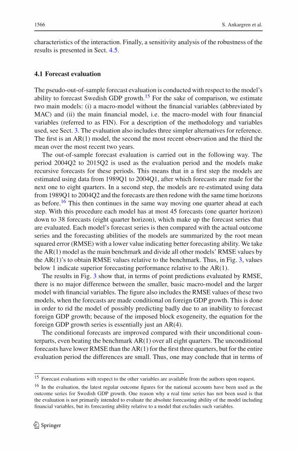
The pseudo-out-of-sample forecast evaluation is conductedwith respect to themodel’sability to forecast Swedish GDP growth.15 For the sake of comparison, we estimatetwo main models: (i) a macro-model without the financial variables (abbreviated byMAC) and (ii) the main financial model, i.e. the macro-model with four financialvariables (referred to as FIN). For a description of the methodology and variablesused, see Sect. 3. The evaluation also includes three simpler alternatives for reference.The first is an AR(1) model, the second the most recent observation and the third themean over the most recent two years.

The out-of-sample forecast evaluation is carried out in the following way. Theperiod 2004Q2 to 2015Q2 is used as the evaluation period and the models makerecursive forecasts for these periods. This means that in a first step the models areestimated using data from 1989Q1 to 2004Q1, after which forecasts are made for thenext one to eight quarters. In a second step, the models are re-estimated using datafrom 1989Q1 to 2004Q2 and the forecasts are then redone with the same time horizonsas before.16 This then continues in the same way moving one quarter ahead at eachstep. With this procedure each model has at most 45 forecasts (one quarter horizon)down to 38 forecasts (eight quarter horizon), which make up the forecast series thatare evaluated. Each model’s forecast series is then compared with the actual outcomeseries and the forecasting abilities of the models are summarized by the root meansquared error (RMSE) with a lower value indicating better forecasting ability. We takethe AR(1) model as the main benchmark and divide all other models’ RMSE values bythe AR(1)’s to obtain RMSE values relative to the benchmark. Thus, in Fig. 3, valuesbelow 1 indicate superior forecasting performance relative to the AR(1).

The results in Fig. 3 show that, in terms of point predictions evaluated by RMSE,there is no major difference between the smaller, basic macro-model and the largermodel with financial variables. The figure also includes the RMSE values of these twomodels, when the forecasts are made conditional on foreign GDP growth. This is donein order to rid the model of possibly predicting badly due to an inability to forecastforeign GDP growth; because of the imposed block exogeneity, the equation for theforeign GDP growth series is essentially just an AR(4).

The conditional forecasts are improved compared with their unconditional coun-terparts, even beating the benchmark AR(1) over all eight quarters. The unconditionalforecasts have lower RMSE than the AR(1) for the first three quarters, but for the entireevaluation period the differences are small. Thus, one may conclude that in terms of

15 Forecast evaluations with respect to the other variables are available from the authors upon request.16 In the evaluation, the latest regular outcome figures for the national accounts have been used as theoutcome series for Swedish GDP growth. One reason why a real time series has not been used is thatthe evaluation is not primarily intended to evaluate the absolute forecasting ability of the model includingfinancial variables, but its forecasting ability relative to a model that excludes such variables.

123


0 1 2 3 4 5 6 7 8 90

0.5

1

1.5

2

Forecast horizon

Rel

ativ

eR

MSE

FIN mod FIN mod, cond MAC modMAC mod, cond Recent mean No change

Fig. 3 Root mean squared errors (RMSE) for predictions of Swedish GDP growth relative to AR(1)

forecasting accuracy, there is in essence no difference between the macro-model andthe financially augmented model.17

The finding in this paper is partly in line with Espinoza et al. (2012). They usedifferent time series models to estimate the importance of financial variables for thereal economy and conclude that financial variables contribute to a better prediction ofeuro areaGDP, especially in 1999 and between 2001 and 2003, when using conditionalpredictive ability tests and a rolling RMSE metric. However, when out-of-sampleforecasts are judged under a static RMSE metric, as is done here, they conclude thatfinancial variables do not help in forecasting real activity in the euro area. This is partlybecause of the assumed identification, in which they isolate the responses of slow-moving variables (the real ones) from that of the fast-moving variables (the financialones) so that the impulse response associated with shocks to financial variables can beseen as marginal impacts beyond what is already accounted for by the real variables.

4.2 Variance decomposition—is there any interaction?

In order to answer our first question, if there is an interaction, we perform a forecasterror variance decomposition. Such a procedure estimates how much of the forecasterror variance of each of the variables can be explained by exogenous shocks to theother variables. The decomposition is presented in Fig. 4. In order to more clearlysee what part can be attributed to the traditional macro-variables and to the financialvariables, the variables are combined into three groups: macro-variables, financialvariables and Swedish GDP growth. The decomposition of the forecast error varianceof Swedish GDP growth, with respect to these groups, is presented in Fig. 5.

17 The forecasts have also been evaluated bymean absolute error and bias, which are available upon request.The results and conclusion from these measures are in line with what is presented here. All models have aminor negative bias, but the size, around −0.2 to −0.4, is similar in size to the AR(1) model’s. However,due to the small sample, one or two larger misses have a quite large effect on the bias calculation.

123


510

1520

0

0. 51

510

1520

0

0.51

510

1520

0

0. 51

510

1520

0

0.51

510

1520

0

0.51

510

1520

0

0.51

510

1520

0

0.51

510

1520

0

0.51

510

1520

0

0.5

0.51

510

1520

0

0.51

510

1520

0

0.51

510

1520

0

0.51

510

1520

0

0.51

510

1520

0

0. 51

510

1520

0

0.51

510

1520

0

0.51

510

1520

0

0.51

510

1520

0

0.51

510

1520

01

510

1520

0

0.51

510

1520

0

0. 51

510

1520

0

0.51

510

1520

0

0.51

510

1520

0

0.51

510

1520

0

0.51

510

1520

0

0.51

510

1520

0

0.51

510

1520

0

0.51

510

1520

0

0.51

510

1520

0

0.51

510

1520

0

0.51

510

1520

0

0.51

510

1520

0

0.51

510

1520

0

0.51

510

1520

0

0.51

510

1520

0

0.51

510

1520

0

0.51

510

1520

0

0.51

510

1520

0

0.51

510

1520

0

0.51

510

1520

0

0.51

510

1520

0

0.51

510

1520

0

0.51

510

1520

0

0.51

510

1520

0

0.51

510

1520

0

0.51

510

1520

0

0.51

510

1520

0

0.51

510

1520

0

0.51

510

1520

0

0.51

510

1520

0

0.51

510

1520

0

0.51

510

1520

0

0. 51

510

1520

0

0. 51

510

1520

0

0.51

510

1520

0

0.51

510

1520

0

0.51

510

1520

0

0.51

510

1520

0

0.51

510

1520

0

0.51

510

1520

0

0.51

510

1520

0

0. 51

510

1520

0

0. 51

510

1520

0

0.51

510

1520

0

0.51

510

1520

0

0.51

510

1520

0

0.51

510

1520

0

0.51

510

1520

0

0.51

510

1520

0

0. 51

510

1520

0

0. 51

510

1520

0

0.51

510

1520

0

0. 51

510

1520

0

0.51

510

1520

0

0.51

510

1520

0

0.51

510

1520

0

0.51

510

1520

0

0.51

510

1520

0

0.51

510

1520

0

0.51

510

1520

0

0.51

510

1520

0

0.51

510

1520

0

0.51

510

1520

0

0. 51

510

1520

0

0.51

510

1520

0

0.51

510

1520

0

0.51

510

1520

0

0.51

510

1520

0

0.51

510

1520

0

0. 51

510

1520

0

0.51

510

1520

0

0. 51

510

1520

0

0.51

510

1520

0

0.51

510

1520

0

0.51

510

1520

0

0.51

510

1520

0

0.51

510

1520

0

0.51

510

1520

0

0.51

510

1520

0

0.51

GDPF

shoc

kSI

shoc

kGDP

shoc

kCPIX

shoc

kU

shoc

kIT

Bsh

ock

LR

shoc

kAGAP

shoc

kCGAP

shoc

kER

shoc

k

GDPF SI GDP CPIX U ITB LR AGAP CGAP ER

Fig.4

Variancedecompo

sitio

n.NoteSh

ocks

have

been

orthog

onalized

usingaCho

leskydecompo

sitio

n,in

which

theordering

istheorderin

which

thevariablesappear

inthefig

ure

123


0

0.25

0.5

0.75

1

Pro

port

ion

Financial variables

0

0.25

0.5

0.75

1Macro variables

Median 68 % 95 %

0 5 10 15 20 0 5 10 15 20 0 5 10 15 200

0.25

0.5

0.75

1Swedish GDP growth

Fig. 5 Median forecast error variance decomposition of GDP with respect to macroeconomic variables,financial indicators and GDP itself

Figure 5 shows that the financial variables are responsible for a non-negligiblepart of the forecast error variance of Swedish GDP growth: in total, they account forapproximately 10%.At around6%, the stress index accounts for the largest share of theforecast error variance of Swedish GDP growth among the financial variables. Thus,the results suggest that financial variables are important for the real economy, but notimmensely so. It shows that it can be important to account for many different aspectsof the transmission channels to get a deeper understanding of the macro-financiallinkages.

This finding is in line with, but smaller than, the findings of the structural DSGEmodels such as Christiano et al. (2014) and Jermann and Quadrini (2012). Chris-tiano et al. (2014) study US macroeconomic data over the period 1985–2010 andconclude that the risk shock (the cross-sectional standard deviation of an idiosyncraticproductivity shock) accounts for a large share of the fluctuations in GDP and othermacroeconomic variables. Jermann andQuadrini (2012) find that financial shocks con-tributed significantly to the observed dynamics of real and financial variables. Morespecifically, they find that changes in credit conditions contributed to the downturns in1990–1991 and 2001 as well as the 2008–2009 recession. Compared to Hubrich et al.(2013), who find a combined effect of five financial shocks on different measures ofoutput to be around 5–45%, the proportion due to financial variables found here islower. Similarly, Adolfson et al. (2013) found, using a DSGE model for Sweden, thatthe shock related to the financial block, which is the entrepreneurial wealth shock intheir model, explains about 3% of the variation in output growth.

As for the reverse relationship, rows 2, 7, 8 and 9 in the third column in Fig. 4display the share of the forecast error variance of the respective row variables that canbe attributed to exogenous shocks to Swedish GDP growth. For the stress index, thelending rate and the asset price gap, Swedish GDP growth appears to be of modestimportance. For the credit gap, however, the share attributable to Swedish GDP growthshocks is around 10–15%. Thus, it seems as if the interaction is two-sided. However,it should be emphasized that the model has been constructed with a certain theoreticalsetting in mind, namely the literature on negative financial externalities and the trans-mission mechanism. The paper thus sets out to answer a one-sided question, namely

123


how the financial system affects the real economy. Although the model seems to indi-cate that Swedish GDP growth affects the credit gap, the model is not constructed toanalyse the determinants of the credit gap or any of the other financial variables for thatmatter. It should of course not be ruled out that the model could be useful in this sense,but any results in this respect should be interpreted with caution. In the sensitivityanalysis in Sect. 4.5, the alternative ordering produces a clear one-sided interaction,which is more in line with the findings in the DSGE literature such as Rabanal andTaheri Sanjani (2015). They show that financial frictions amplified economic fluc-tuations and the measure of the output gap in all euro countries except France andGermany. On the contrary, in France and Germany financial frictions played a minorrole in output gapmeasures. Financial frictionsmatteredmuchmore precisely becausefinancial and housing demand shocks are the ones that set the financial accelerator inmotion, and those shocks were more important in all euro countries except France andGermany.

To conclude this section, an interaction appears to exist as we find that financialshocks are responsible for approximately 10% of the forecast error variance decom-position of Swedish GDP growth. The results indicate that a financial stress shockis of particular importance to the real economy. In the opposite direction, a SwedishGDP growth shock appears to be of more importance to the forecast error varianceof credit gap than to the forecast error variance of the other financial variables, withan attributable proportion of around 15%. It should again be noted that the orderingof the variables affects the result. The sensitivity analysis in Sect. 4.5 reveals that analternative ordering alters the conclusion somewhat, although the main conclusionof the existence of a linkage remains intact. Indeed, it is in fact strengthened by thealternative ordering.

4.3 Recession probabilities—can the interaction help us make betterpredictions?

In this subsection, we study the models’ implied probabilities of recession. Österholm(2012) performs an alternative forecasting exercise with a steady-state BVAR for theUSA. Standing in 2008Q2, the focus of the paper is the model’s estimated probabilityof a coming crisis, with a crisis defined as two consecutive quarters of negative GDPgrowth. We take the same approach and let the recession probability at time t bedefined as the probability of negative Swedish GDP growth at both time t + 1 andt + 2. The probability is estimated by computing the proportion of draws in thenumerical simulation of the model in which the unconditional forecasts of SwedishGDP growth in t +1 and t +2 are negative. We calculate the probability over the timeperiod 2004Q1 and 2015Q1 for both the macro- and the financial models.18

Before commenting on the results in Fig. 6, it is important to stress that the exerciseshould not be interpreted as intended to compete with the large literature on early

18 We have also generated the model’s predicted probability of a coming crisis between 2004Q1 and2015Q1, with a crisis defined as one quarter of negative growth. The estimated probability is even betterwhen the model only needs to estimate one quarter. These estimates are available upon request.

123


2004 2006 2008 2010 2012 20140

0.1

0.2

0.3

0.4

0.5

0.6

0.7

Year

Pro

babi

lity

of r

eces

sion

Negative growth Financial modelMacro model

Fig. 6 Future recession probabilities. NoteA future recession is defined as negative growth in the next twoquarters

warning indicators.19 Furthermore, such indicators are usually economic or financialvariables or the product of a relatively simple model. Rather, the measure of recessionprobability in this paper comes from a model trying to incorporate the transmissionmechanism within a macro-model. The probability measure is the product of macro-and financial developments, interpreted in a reduced formmodel of the economy. Thus,the relevant benchmark is whether or not the financial model is better at signallingshort-term recession risk than is the traditional macro-model.

Beginning in 2007 and ending right before the crisis unfolded in 2008Q3, bothmodels’ probabilities of recession steadily increase. The financial model shows amore rapid increase, but up through 2008Q1, the two models’ estimated probabilitiesare more or less the same. However, standing in 2008Q2—right before Sweden startedexperiencing negative growth—the financial model’s probability of negative growthin both 2008Q3 and 2008Q4 is 16%, whereas the corresponding estimate from themacro-model is 7%. One could argue that given the lag in response, this indicatorwould not be an informative leading indicator. However, as mentioned earlier, thisindicator produced a clear signal one to two quarters before the global financial crisishit the Swedish economy.

Beginning in late 2010, the probability of a recession is again slowly increasingfollowing the events leading up to the intensification of the Eurozone crisis, with theEuropean Central Bank reactivating its Securities Markets Program in August 2011.This is directly reflected in the financial model’s estimated recession probability, butis at the same time barely visible in the macro-model’s because of its lack of financialvariables. This indicates that the more complete picture given by the inclusion offinancial variables is important, as it provides information about the developments inthe financial markets, which are likely to eventually transmit into the real sector.

19 A recent example is López-Salido et al. (2016).

123


These findings are also in line with Fornari and Lemke (2010). The authors use aprobit regression model linked to a VAR model, a so-called ProbVAR model, to gen-erate conditional recession probabilities and conclude that forecasts can be markedlyimproved by adding financial variables to this model. It is encouraging that our resultsagree with Fornari and Lemke (2010) in the sense that financial variables appear tobe highly useful and informative. One conclusion from the finding in this paper aswell as previous findings is that accounting for financial variables in the episode ofa financial crisis enhances model fit and statistical indicators such as probability ofrecession, compared to the model that does not have a way to systematically accountfor the financial variables.

One way to complete the recession probability analysis in this paper is to make acareful analysis of the financial variables included in the model. López-Salido et al.(2016) argue that elevated credit market sentiment at year t − 2 (proxied by thepredicted year-t change in the credit spread) is associated with a decline in economicactivity in years t through t + 2.20 That is, when their sentiment proxies indicate thatcredit risk is aggressively priced, this tends to be followed by a subsequent wideningof credit spreads, and the timing of this widening is, in turn, closely tied to the onsetof a contraction in economic activity. One way to further develop the model in thispaper is to include the credit market sentiment in financial stress index instead of TEDspread and mortgage bond spread.21 This is left as a suggestion for future research.

4.4 Conditional forecasts—can the interaction improve our estimates of crisiseffects?

Another way of analysing whether there is any potential gain of including financialvariables in the model is by conditioning on them to investigate how the forecastschange had we known their developments. In particular, it is illustrative to make fore-casts before the crisis fully developed and compare the predictions from the financialmodel, conditional upon the financial variables, with the macro-model’s predictions.If the model is reasonably constructed, it should to some degree signal that times areworsening if we condition upon the financial development during the crisis. The con-ditional forecasts in this subsection are reminiscent of the conditional predictions inBanbura et al. (2015) and Espinoza et al. (2012). As also pointed out by these authors,in the current setup conditional forecasts are created by shocking the system in sucha way that the conditioning path is satisfied, which imposes restrictions on the errors.Contrary to Banbura et al. (2015), shocks are produced in a structural representationof the model and then transformed to the reduced form.22 For this reason, the ordering

20 The credit spread is measured by the spread between yields on seasoned long-term Baa-rated industrialbond and yields on comparable-maturity Treasury securities.21 Another way to do this is to divide the financial stress index to two different stress indices: one thatcapture the volatility at the stock and currency markets and one that captures the spreads in the money andbond market. In that case, the spread for the bond market can be replaced by the credit market sentiment.22 The method is similar to that used by Adolfson et al. (2005). More specifically, the procedure at forecasthorizon h is as follows: 1) shocks for the macroeconomic variables are drawn from their estimated distri-

123


2008 2009

4

2

0

2

Ann

ualG

DP

grow

th

Outcome Forecast at 2007Q4 Forecast at 2008Q1 Forecast at 2008Q2

Fig. 7 Financial model’s forecasts of annual GDP growth in 2008 and 2009. Note The forecasts are madeconditional upon the financial indicators and foreign GDP growth during 2008 and 2009

of the variables will affect the results as the transformations are based on a recursiveidentification scheme.

This hypothetical exercise is carried out as follows. The two models are estimatedusing data up to and including 2007Q4. Both models make out-of-sample conditionalforecasts of Swedish GDP growth in 2008 and 2009 by transforming the quarterlyforecasts to annual growth. The financial model’s forecasts are conditional on the out-comes of foreign GDP growth and the four financial variables in 2008Q1–2009Q4 andthe macro-model’s forecasts are conditional on the outcome of foreign GDP growththroughout the same period. Next, data for 2008Q1 are added to the estimation sam-ple and the out-of-sample conditional forecasting repeated (conditional on outcomesin 2008Q2–2009Q4). Lastly, the same task is repeated a third time using also datafor 2008Q2 in the estimation (with forecasts conditional on outcomes in 2008Q3–2009Q4). Thus, the exercise results in three forecasts for 2008 and three forecasts for2009 for each model, with each forecast triple containing forecasts using increasingamounts of information in the estimation.

Figures 7 and 8 display the financial and macro-models’ predictions for annualgrowth in 2008 and 2009, respectively. As expected, the financial model providesforecasts that are more in line with the outcomes. In Fig. 7, for the model estimatedat 2007Q4 the negative growth in 2008 is not anticipated, but a downturn in 2009is predicted, although not the full size of it. Estimating the model at 2008Q1 and2008Q2 gives more pessimistic forecasts that are closer to the outcome. This should becontrasted to Fig. 8 and themacro-model’s predictions. The pattern ofmore pessimisticpredictions as the estimation sample is increased persists, but they are markedly moreoptimistic at around −1.5% than the financial model’s at around −3%. A differenceof 1.5 percentage points might at a first glance seem small, but could be viewed inlight of the small differences in unconditional forecasts (see Table 2). Another way of

butions, 2) a shock to foreign GDP growth is injected such that it satisfies its condition and 3) given theprevious shocks, financial shocks are drawn to make the financial variables meet their conditions.

123


2008 2009

4

2

0

2

Ann

ualG

DP

grow

th


Fig. 8 Macro-model’s forecasts of annual GDP growth in 2008 and 2009. Note The forecasts are madeconditional upon foreign GDP growth during 2008 and 2009

describing the 1.5% point difference is to relate it to the long-run average of SwedishGDP growth, which stands at approximately 2% for the sample used in this paper(1989Q1 to 2015Q2). Yet another is to relate the 1.5 percentage point difference tothe standard deviation of the series, which is 0.93. Summing up, the financial model’sprediction of Swedish GDP growth in this exercise seems to be better compared to themacro-model’s forecast.23

These forecasts illustrate what is perhaps the greatest advantage of augmentinga traditional macro-model with financial variables. With the financial model, it ispossible to carry out forecasts that are conditional on developments in the financialsystem, an exercise that is of particular interest when these exhibit increased volatility.

As discussed in the identification section (Sect. 3.3), these forecasts are dependentupon the ordering of the variables. For this reason, in the sensitivity analysis (seeSect. 4.5) we consider an alternative ordering and redo the preceding forecastingexercise.

The conditional forecast exercise in this subsection is generally in line with thefindings in IMF (2015), Banbura et al. (2015) and Espinoza et al. (2012). IMF (2015)analyse how balance sheets of households and non-financial corporations affect theeconomic outlook using a BVAR model. They find that using balance sheet informa-tion improves the forecast of aggregate activity when applied to the USA. In addition,shocks to balance sheets are also found to have a significant and differentiated eco-nomic impact, suggesting that balance sheets carry additional information. Banburaet al. (2015) also use a BVAR model, as well as a large dynamic factor model, toestimate the interaction between 26 euro area macroeconomic and financial variables.They find that the two approaches generally deliver similar forecasts and scenario

23 While the median forecast may be close to the realization, it may be associated with large uncertainties.For this reason, we have also compared prediction intervals from the models. The financial model’s predic-tion intervals are generally wider, but only by 5–15%. The complete results are available from the authorsupon request.

123


assessments. Their conditional forecast exercise is similar to ours, but instead theycondition on real GDP, consumer prices and short-term interest rates. Interestingly,the forecasts are generally in line with the outcomes, with the exception of loans tohouseholds and firms where the major downturn is not fully anticipated. In our case,the situation is the opposite since we condition upon the financial variables to makeimproved forecasts of the growth of GDP. Espinoza et al. (2012) find similar, improvedresults when forecasting ability is assessed as if in real time. In their base line model,however, financial variables does not provide any extra information to their modelwhere euro area GDP growth is explained by the USA and Rest of the World GDPgrowth. In short, the literature on conditional forecasts seems to find some evidence ofa two-way macro-financial linkage, although the amount of research still is too limitedto allow for any strong conclusions in this respect.

4.5 Sensitivity analysis

We investigate the robustness of the results by conducting a sensitivity analysis. Thisis done in two parts. In the first part, the specifications in the prior are changed oneby one, changing the ordering of the variables and also considering the Minnesotaprior (i.e. without an informative prior on the steady state). We check the robustnessby studying how future forecasts and the forecast error variance decompositions after20 periods change. In the second part, we select one alternative ordering and rerun theanalysis in full with the alternative ordering to investigate the sensitivity of the resultsto our particular choice.

The first part includes changing the hyperparameters λ1, λ2 and λ3, relocating thecentre of the prior probability intervals for the steady states and also extending thewidth of the prior intervals for the steady states. All changes are done one by one.Finally, we elaborate with alternative identification assumptions, where the financialvariables are added after the macro-variables, to see how important the identificationassumption is for the results.

The first two hyperparameters λ1 and λ2 are increased so as to relax the informa-tiveness of the prior. The lag decay parameter, λ3, is also increased, but this has theopposite effect of a tighter prior. For the steady-state priors, we consider two typesof changes. First, we let all prior probability intervals keep their length, but shifttheir centre upwards by one standard deviation. Second, the prior probability intervalsremain centred on the same values, but the length of the intervals is doubled. Thesetwo changes will give us some idea of how the results are affected by the locationand the tightness of the steady-state priors. We also investigate sensitivity with respectto the ordering of the variables. Three alternative orderings are considered, in which1) the financial stress index is moved to the second-to-last position, 2) most of thefinancial variables come first and Swedish GDP growth is last and 3) asset price gapand credit gap are moved to come prior to the stress index. By doing this, the hopeis to gain an understanding of how important the ordering actually is. The results aredisplayed in Table 2.

Table 2 suggests that with respect to the choices for the prior, the results seem tobe insensitive. The future forecasts and the forecast error variance decompositions

123


Table 2 Sensitivity analysis

Prior changed Forecasts of annual GDP growth FEVD of GDP, 20 periods

2015 2016 2017 2018 2019 Macro Financial GDP

Baseline 2.97 3.34 2.90 2.59 2.33 0.37 0.10 0.53

λ1 3.06 3.46 2.82 2.53 2.33 0.45 0.14 0.41

λ2 3.03 3.38 2.84 2.57 2.35 0.43 0.13 0.44

λ3 2.94 3.30 2.94 2.63 2.37 0.35 0.08 0.57

GDPF Mean 2.98 3.33 2.87 2.62 2.36 0.37 0.10 0.53

CGAP Mean 2.96 3.32 2.91 2.62 2.39 0.37 0.10 0.53

AGAP Mean 2.98 3.32 2.87 2.56 2.33 0.37 0.10 0.53

LR Mean 2.98 3.33 2.87 2.61 2.35 0.37 0.10 0.53

SI Mean 2.97 3.31 2.83 2.51 2.26 0.38 0.10 0.53

ITB Mean 2.98 3.30 2.84 2.56 2.32 0.37 0.10 0.53

ER Mean 2.99 3.37 2.92 2.61 2.33 0.37 0.10 0.53

CPIX Mean 2.97 3.36 2.90 2.61 2.35 0.37 0.10 0.53

UNEMP Mean 2.98 3.36 2.91 2.61 2.36 0.37 0.10 0.53

GDP Mean 2.97 3.33 2.88 2.58 2.33 0.37 0.10 0.53

GDPF SD 2.98 3.38 2.95 2.61 2.35 0.38 0.10 0.52

CGAP SD 3.01 3.41 2.87 2.56 2.32 0.38 0.10 0.53

AGAP SD 3.01 3.52 3.11 2.84 2.59 0.37 0.10 0.53

LR SD 2.97 3.37 2.93 2.61 2.34 0.37 0.10 0.53

SI SD 2.97 3.27 2.78 2.47 2.24 0.37 0.10 0.53

ITB SD 2.98 3.42 2.98 2.66 2.34 0.38 0.10 0.52

ER SD 2.99 3.38 2.92 2.61 2.35 0.37 0.10 0.53

CPIX SD 2.97 3.34 2.93 2.62 2.40 0.37 0.10 0.53

UNEMP SD 2.98 3.36 2.93 2.60 2.32 0.37 0.10 0.53

GDP SD 2.98 3.32 2.85 2.55 2.32 0.37 0.10 0.53

Order 1 2.98 3.35 2.87 2.61 2.36 0.39 0.07 0.54

Order 2 2.98 3.34 2.86 2.58 2.33 0.38 0.25 0.37

Order 3 2.98 3.37 2.88 2.57 2.30 0.36 0.22 0.42

Minnesota 2.90 3.00 2.65 2.56 2.55 0.36 0.10 0.54

The hyperparameters λ1, λ2 and λ3 are changed to 0.5, 1 and 2, respectively. The “Mean” row entires aresubject to a one standard deviation upward shift of the mean of the prior. The “SD” row entries are subjectto a doubling of the prior 95% probability interval. At the end of the table, the ordering of the variables isreshuffled. Order 1 is (GDPF, GDP, CPIX, U, ITB, IL, AGAP, CGAP, SI, ER), Order 2 is (GDPF, CGAP,AGAP, IL, ITB, SI, ER, CPIX, U, GDP) and Order 3 is (GDPF, AGAP, CGAP, SI, GDP, CPIX, U, ITB, IL,ER). Lastly, the model is estimated with theMinnesota prior instead of the steady-state prior. The first blockof columns displays the annual forecasts of GDP growth of the coming years. The second block displaysthe proportion of the forecast error variance decomposition of GDP 20 periods ahead, which is attributableto the macroeconomic variables, the financial variables and Swedish GDP growth itself, respectively

123


are all similar when we change the hyperparameters and the centre and lengths ofthe prior probability intervals. Using the alternative orderings does not affect thefuture forecasts, as expected. When using the first alternative ordering of variables,i.e. when the stress index is moved, also the forecast error variance decompositionsremain close to the main results. However, when considering the second or thirdalternative ordering, the contribution to the forecast error variances which is due tofinancial shocks increases from 10 to 22 and 25%, respectively. By the nature ofthe new orderings, this is hardly surprising; both of them place financial variables(other than just the stress index) prior to Swedish GDP growth. As discussed in, forexample, Eichenbaum and Evans (1995), this means that we are implicitly assumingthat the preceding financial variables are causally prior to it. In our main ordering,only the stress index is assumed to be causally prior to Swedish GDP growth. Forthis reason, the second and third orderings illustrate the fact that as more financialvariables are assumed to be causally prior to it, the share of forecast error variancesattributable to these variables increases. Using the Minnesota prior leaves the forecasterror variance decompositions virtually unchanged, but the trajectory of the futureforecast is somewhat flatter.

In the second part of our sensitivity analysis, we redo the entire statistical analysiswith a new ordering. However, since most of the results are not dependent on theordering, only the parts which change, i.e. the conditional forecast exercise and theforecast error variance decompositions, are presented here.

The alternative ordering considered is based on moving the asset price and creditgaps from positions 8 and 9 to positions 2 and 3, i.e. placing them first among thedomestic variables. There are two main reasons for doing so. The results are mostsensitive to moving variables in the conditioning to positions before Swedish GDPgrowth. Thus, if the results change, the induced change will likely be among thelarger changes that can occur by simply reordering the variables. Additionally, theconsequence of this reordering in a recursive setting is that the two gap series willonly react to all other domestic variables with a lag. Given their persistent nature, sucha slow reaction is sensible.

Since the internal ordering of the macro-variables is unchanged, the macro-model’sforecasts are also unchanged and therefore not displayed here (instead, see Fig. 8).The results of the conditional forecasts with the alternative ordering are displayed inFig. 9.

As seen in Fig. 9, the effect of changing the order of the variables is substantial.The forecast of annual Swedish GDP growth in 2009 made in 2007Q4 is almost 2percentage points lower than with the main ordering (see Fig. 7). Overall, the modelseems to be more responsive to the signals in the financial variables. This result hasa number of implications. First, it means that the ordering is a non-trivial task, whichaffects the end result. Second, it implies that not only the choice of included variables isimportant for the model’s performance, but also the (explicitly or implicitly) assumedinteractions, which hardly is surprising. However, it does not necessarily constitute aproblem. With a more elaborate and careful identification strategy, with identificationbeing a main focus rather than a necessary by-product of the analysis, one couldpossibly obtain an even better performance of the model. This is also the case for thesteady-state priors. From time to time, structural changes may change the steady-state

123


2008 2009

4

2

0

2

Ann

ualG

DP

grow

th


Fig. 9 Financial model’s forecasts of annual GDP growth in 2008 and 2009. Note The forecasts are madeconditional upon the financial indicators and foreign GDP growth during 2008 and 2009, but with a differentordering than in Fig. 4

assumptions given as priors in Table 1.With more elaborate and carefully chosen priorbeliefs, one could possibly obtain even better performance of the model because of thestructural changes.24 Furthermore, it would be highly interesting to incorporate non-linearities in this context as well. It is plausible that the relationships are not constantover time, as implicitly assumed here, but change. For example, if the conditioningpaths in some sense suggest crisis times, the model itself may need to change. To someextent, this is achieved here by changing the ordering of the variables. This could thensuggest that different identifications may be useful at different times. Such nonlinearmacro-financial linkages are discussed in detail by Hubrich et al. (2013).25 However,Fornari and Stracca (2013) provide some evidence of the non-linearities being absentby estimating their model with and without crisis times and noting that the results arefairly stable.

5 Conclusion and comments

The purpose of this paper has been to answer two main questions: (i) Is the financialsystem important for the development in the real economy? (ii) If it is, what are thecharacteristics? After estimating a BVAR model for the macroeconomy, augmentedwith financial variables representing the transmission mechanism, a decomposition ofthe forecast error variance of Swedish GDP growth reveals that the financial shocksexplain 10–25% of the variance, depending on the chosen identification. As mightbe expected, an ordering where the financial variables come first generates the higherforecast error variance.

24 Fornari and Stracca (2013), for example, consider sign restrictions as in Rubio-Ramírez et al. (2010).A similar approach could be taken here.25 In addition, such an identification pursuit and steady-state prior choices could also possibly mitigate therelevance of the Lucas’ critique.

123


To see the characteristics of the financial-to-real interaction, two differentapproaches were used. First, financial variables were included to see whether thisimproved the model’s ability to estimate recession probabilities and second, condi-tional forecasts were used to quantify the effects on SwedishGDP growth of a financialcrisis. The results indicate that the financialmodel, to a larger extent than themacroeco-nomic model, acknowledges the increasing distress preceding the crisis. The financialmodel’s estimated probability of a recession is stronger at an earlier date than themacroeconomic model’s, thus connecting the financial turmoil to greater uncertaintysurrounding the growth of the economy. Second, and more importantly, the financialmodel produces a more accurate forecast of the depth of the 2008–2009 crisis in Swe-den, when comparing forecasts made in the quarters just before the outbreak of thecrisis. Conditional on the financial variables, the model’s forecast of Swedish GDPgrowth over the coming two years is clearly lower—and thus more accurate—thanthe macro-model’s forecast. In the alternative ordering of variables tried in the sen-sitivity analysis, the advantage of conditioning on the financial variables is furtheraccentuated.

Furthermore, this increase in explanatory power does not come at the expenseof lower predictive power. There is no loss to point predictions, in terms of rootmean squared error (RMSE), by expanding a traditional macroeconomic model withfinancial variables. Compared with the traditional macroeconomic model, there is nodifference as to their unconditional forecasting performances.

Concluding, the proposed macro-financial model fills a gap in the literature byproviding an empirical model that can be used to analyse and forecast the impact thatdevelopment of the financial sector may have on the real economy.

For future research, there are many interesting extensions one could make. Theinclusion of stochastic volatility in the steady-state prior, as proposed by Clark (2011),appears to be a promising alternative. Similarly, allowing the model to have time-varying or regime-switching parameters could be interesting ways of incorporatingnon-linearities, which might improve the model even further.

Acknowledgements Wewould like to thank Thomas Bergman, Per Englund, Torbjörn Halldin andMartinSolberger and the seminar participants at theMinistry of Finance and theDepartment of Statistics at UppsalaUniversity, three anonymous referees, and two editors for useful suggestions and discussions. A specialthanks to John Hassler, Pehr Wissén, Lars E O Svensson, Peter Englund, Mats Kinnwall, Lars Hörngren,Johan Lyhagen, Fredrik Bystedt, Albin Kainelainen and Robert Boije for valuable comments on an earlierdraft of the paper and to Mattias Villani for allowing us to use his code. The views expressed in this paperare solely the responsibility of the authors and should not necessarily be taken to reflect the views of theSwedish National Debt Office and the Ministry of Finance.

Open Access This article is distributed under the terms of the Creative Commons Attribution 4.0 Interna-tional License (http://creativecommons.org/licenses/by/4.0/), which permits unrestricted use, distribution,and reproduction in any medium, provided you give appropriate credit to the original author(s) and thesource, provide a link to the Creative Commons license, and indicate if changes were made.

123

http://creativecommons.org/licenses/by/4.0/


Appendix: The theoretical effects of the financial system on the realeconomy

We start by giving a detailed description of the way negative external effects causethe accumulation and liquidation of financial imbalances. Next, we present a com-prehensive but tractable description of the transmission mechanism and its channels.Finally, we describe the way the identified negative externalities affect the real econ-omy through the different transmission channels

Negative externalities and financial imbalances

The importance of the financial shocks and financial frictions is well summarized inBrunnermeier et al. (2012). They point out that external funding is typically moreexpensive than internal funding through retained earnings. This implies that agentsto a large extent issue claims in the form of debt which comes with some severedrawbacks: an adverse shock wipes out large fraction of the levered borrowers networth, limiting his risk bearing capacity in the future. Hence, a temporary adverseshock is very persistent since it can take a long time until agents can rebuild their networth through retained earnings. Besides persistence, an initial shock is amplified ifagents are forced to resell their capital. Since resales depress the price of capital, thenet worth of agents suffers even further (loss spiral). In addition, margins and haircutsmight rise (loan-to-value ratios might fall) forcing agents to lower their leverage ratio(margin spiral).

The persistence of a temporary shock lowers future asset prices, which in turn feedback to lower contemporaneous asset prices, eroding productive agents’ net wortheven further and leading to more resales which can lead to rich volatility dynamicsand explain the inherent stability of the financial system.Because of thesemechanisms,credit risk can be dwarfed by liquidity risk and cause a large discontinuous drop inthe price level and a dry-up of funding.

The role of financial institutions is to mitigate some of these financial frictions.However, by investing in long-term projects and by issuing short-term debt claims,financial institutions expose themselves to a liquidity mismatch, which can result infragility. Banks can also ensure that the borrower of funds exerts enough effort suchthat loans can be repaid. Moreover, Banks can also create securities and offer depositcontracts. However, by doing so, they expose themselves to bank runs. Financialintermediaries are thus key in understanding the interaction between financial systemand real economy. Brunnermeier et al. (2012), Shin (2010) and Hanson et al. (2011),among others, argue that financial institutions do not take adequate account of thecontagion effects of their behaviour on the financial system and the real economy.

Predatory pricing of risk, herd behaviour and the moral hazard in combination withthe implicit safety netmay over time lead to financial imbalances. A correction of theseimbalances propagates rapidly through thefinancial systembecause of the linkages thatexist between the various financial institutions. Fire sale is another negative externalitythat leads to asset prices fall even more and affect other institutions with similarassets (e.g. Kashyap et al. 2011). In addition, financial institutions have much more

123


Credit/GDP

Time Phase 1 Phase 2 Phase 3

Asset price and leverage spiral

Interconnectedness

Fire sale

Credit crunch

Balance sheet consolidation

Strategic complementarities

Pure informational contagion

Agents: Banks, households and compnies Banks Households and companies

Fig. 10 Most important negative external effects in a stylized credit cycle

difficulties to roll over their short-term interbank funding (Perotti and Suarez 2009).What matters in the end is perhaps not the boom or the asset price bubble in itself,but rather whether the boom is financed by credit from leveraged institutions (Croweet al. 2011).

For the purpose in this paper, we use the framing of externalities presented anddiscussed inDeNicolò et al. (2012). The negative externalities are illustrated in Fig. 10in a stylized credit cycle.26

In phase 1 of the credit cycle, GDP growth is usually high and the situation ischaracterized by rapidly rising credit volumes and asset prices, for both real andfinancial assets. This phase involves banks, households and firms taking on increasingamounts of debt, an increase in the risk associated with over-borrowing and in increasein risk correlation. Phase 2 originates when a financial crisis is triggered. On the backof falling asset prices, the banks experience capital adequacy problems, which must beremedied. Phase 2 means that banks liquidate large parts of the financial imbalancesthat were built up during phase 1. In phase 3, the mechanisms behind the problem arevery similar to those driving the banks in phase 2, i.e. balance sheet restructuring byfirms and households. It should be emphasized that the above description is schematic.Phase 2 need not be preceded by phase 1, and phase 3 need not be preceded by phases1–2, which constitute another argument for a broad approach.

26 The choice of three phases is made mainly on pedagogical grounds and should not be seen as in contrastor as an alternative to earlier corner stones in the literature, e.g. Minsky (1992) and Kindleberger (2000).Footnote 26 continuedThus, this paper’s naming and numbering of the phases is not the main issue, rather the stylized credit cycleshould be viewed as a link between the negative externalities and the transmission channels.

123


The transmission channels

The financial system mainly affects the real economy through the following transmis-sion channels: the balance sheet channel, the interest rate channel, the bank capitalchannel and the uncertainty channel.27

The balance sheet channel describes how falling asset prices, e.g. house pricesand stock prices, reduce the value of assets held by households and businesses.28

If the value of assets used as security for loans falls, lenders can tighten collateralrequirements at the same time as the loan terms get worse, e.g. because the lendingrate is higher or because the borrower is not allowed to borrow as much as they maywant to. Next, this weighs even further on asset prices, leading to a financial acceleratoreffect and ultimately to a slowdown in consumption and investment.

The interest rate channel describes how the real economy is affected when marketinterest rates rise, for example because the central bank increases the repo rate. Risingmarket interest rates lead to higher financing costs for banks and consequently tohigher lending rates.29 This, in turn, leads to a slowdown in consumption/investmentsby households/businesses.30 can have a negative effect on the price of financial andreal assets because the present value of future returns from these assets decreases.Consumption also decreases as a result of this wealth effect.

The bank capital channel describes how different types of risk associated with theoperations of banks (e.g. market risk, credit risk and financing risk) worsen bankbalance sheets by, for example, reducing the value of the bank’s assets and equity.31

However, banksmustmeet certain requirements concerning capital adequacy, solvencyand liquidity. Banks can choose to either raise their lending rates (thereby increasingtheir profit and equity) and/or reduce their lending to be able to fulfil these requirementswhich lead to lower consumption and less investment.

The uncertainty channel describes howmore uncertainty in the form of price fluctu-ations in financial markets, i.e. greater volatility, leads to higher precautionary savingsand lowers consumption as well as less investment.32

27 The interested reader is referred toBaselCommittee (2011, 2012a, b);Antony andBroer (2010);Ministryof Finance (2013); Gerke et al. (2012) for summaries of the latest research in this area.28 Along with the interest rate channel, it is also called the credit channel. See, for example, Bernanke andGertler (1989); Bernanke et al. (1998); Kiyotaki and Moore (1997); Holmström and Tirole (1997).29 In principle, the policy rate is assumed to have an immediate effect on short-termmarket rates and laggedeffect on long-term rates.30 Monetary policy can also affect the economy via the “exchange rate channel”. An increase in the policyinterest rate normally leads to exchange rate appreciation. A stronger exchange rate means lower importprices, with the result that some domestic demand moves from domestic to imported goods. This moderatesthe inflationary pressure and also leads to a weaker balance of trade. Moreover, monetary policy also affectsthe economy through other channels via expectations.31 See, for example, Stein (1998) and Heuvel (2002, 2004).32 See, for example, Antony and Broer (2010).

123


Weaker balance sheets

Loans more expensive

Weaker balance sheets and worsening cash flow

(Households and companies)

Weaker consumption/investment

Falling asset prices,

rising interest rates

BAN

KS

FIN

AN

CIA

L

MARK

ETS

REAL

ECO

NO

MY

Increasing

market, liquidity

and credit risk

BORR

OW

ERS

Higher

volatilityA

A

B

C

D

A

A

B

B

B

BC

C

D

D

Balance sheet channel

Uncertainty channel

Interest rate channel

Bank capital channel

C

Fig. 11 Transmission mechanism flow chart, including the three main areas of the credit cycle’s negativeexternal effects

The linkages between negative externalities and transmission channels

The negative external effects can also be described in terms of their effect on threemainareas of the economy: (i) market liquidity, (ii) the supply of credit and (iii) the demandfor credit. Depending on the channel, the effects go via the financial markets, the banksand/or households and firms before finally affecting the real economy. Dividing thenegative externalities into these three main areas allows us to illustrate how they affectthe real economy through various transmission channels as illustrated in Fig. 11. Thedifferent transmission channels in the economy have been marked by letters A to D inthe figure; (A) the interest rate channel; (B) the bank capital channel; (C) the balancesheet channel; and (D) the uncertainty channel.33

Information contagion and fire sales are typical externalities affecting market liq-uidity during phase 2, characterized by major volatility and rapid general declines in

33 Figure 8 is schematic and should not be interpreted as saying that the four transmission channels areindependent of one another.

123


financial markets. Heightened volatility leads to increased uncertainty and is followedby greater caution, thus curbing demand in the economy (the uncertainty channel).

The effects on the supply of credit occur in both phase 1 and phase 2, and intensifythe upturn or downturn. In phase 2, a higher degree of interconnectedness betweenfinancial institutions intensifies the shocks, which exacerbates the credit contractionor results in higher lending rates. This, in turn, leads to a fall in demand in the realeconomy (bank capital channel).

The effects on the demand of credit occur in both phase 1 and phase 3 but isperhaps most tangible in phase 3 when households and firms react to the decline inasset prices. In order to reduce their debt ratio, households increase their precautionarysaving, which reduces aggregated demand in the economy (the balance sheet channel).

References

Abildgren K (2012) Business cycles and shocks to financial stability: empirical evidence from a new set ofDanish quarterly national accounts 1948–2010. Scand Econ Hist Rev 60:50–78

Adalid R, Detken C (2007) Liquidity shocks and asset price boom/bust cycles. Working Paper No. 732,European Central Bank

Adolfson M, Laséen S, Lindé J, Villani M (2005) Are constant interest rate forecasts modest policy inter-ventions? Evidence from a dynamic open-economy model. Int Finance 8:509–544

Adolfson M, Andersson M, Lindé J, Villani M, Vredin A (2007) Modern forecasting methods in action:improving macroeconomic analyses at central banks. Int J Cent Bank 3:111–144

Adolfson M, Laséen S, Christiano L, Trabandt M, Walentin K (2013) Ramses II—Model description.Occasional Paper No. 12, Sveriges Riksbank

Antony J, Broer P (2010) Linkages between the financial and the real sector of the economy: a criticalsurvey. CPB Document No. 216, CPB Netherlands Bureau for Economic Policy Analysis

Arregui N, Benes J, Krznar I, Mitra S, Santos AO (2013) Evaluating the net benefits of macroprudentialpolicy: a cookbook. Working Paper No. 13/167, International Monetary Fund

BanburaM, Giannone D, Reichlin L (2010) Large Bayesian vector auto regressions. J Appl Econom 25:71–92

Banbura M, Giannone D, Lenza M (2015) Conditional forecasts and scenario analysis with vector autore-gressions for large cross-sections. Int J Forecast 31:739–756

Basel Committee on Banking Supervision (2011) The transmission channels between the financial andreal sectors: a critical survey of the literature. BCBS Working Paper No. 18, Bank for InternationalSettlements

BaselCommittee onBankingSupervision (2012a)Thepolicy implications of transmission channels betweenthe financial and the real economy. BCBS Working Paper No. 20, Bank for International Settlements

Basel Committee on Banking Supervision (2012b) Models and tools for macroprudential analysis. BCBSWorking Paper No. 21, Bank for International Settlements

Bernanke B, Gertler M (1989) Agency costs, net worth and business fluctuations. Am Econ Rev 79:14–31Bernanke B, Gertler M, Gilchrist S (1998) The financial accelerator in a quantitative business cycle frame-

work. Working Paper No. 6455, National Bureau of Economic ResearchBloom N (2009) The impact of uncertainty shocks. Econometrica 77:623–685Bloom N, Floetotto M, Jaimovich N, Saporta-Eksten I, Terry S J (2012) Really uncertain business cycles.

Working Paper No. 18245, National Bureau of Economic ResearchBrunnermeier K, Eisenbach M T, Sannikov Y (2012) Macroeconomics with financial frictions: a survey.

Working Paper No. 18102, National Bureau of Economic ResearchChristiano LJ, Eichenbaum M, Evans CL (1996) The effects of monetary policy shocks: evidence from the

flow of funds. Rev Econ Stat 78:16–34Christiano LJ, Eichenbaum M, Evans CL (1999) Monetary policy shocks: What have we learned and to

what end? In: Taylor JB, Woodford M (eds) Handbook of macroeconomics, vol I. North-Holland,Amsterdam, pp 65–148

Christiano LJ, Motto R, Rostagno M (2014) Risk shocks. Am Econ Rev 104:27–65

123


Clark T (2011) Real-time density forecasts from Bayesian vector autoregressions with stochastic volatility.J Bus Econ Stat 29:327–341

Crowe C, Dell’Ariccia G, Igan D, Rabanal P (2011) Policies for macrofinancial stability: options to dealwith real estate booms. Staff Discussion Notes No. 11/2, International Monetary Fund

De Nicolò G, Favara G, Ratnovski L (2012) Externalities and macroprudential policy. Staff DiscussionNotes No. 12/5, International Monetary Fund

Drehmann M, Borio C, Gambacorta L, Trucharte C (2010) Countercyclical capital buffers: exploringoptions. Working Paper No. 317, Bank for International Settlements

Eichenbaum M, Evans CL (1995) Some empirical evidence on the effects of shocks to monetary policy onexchange rates. Q J Econ 110:975–1009

Espinoza R, Fornari F, Lombardi MJ (2012) The role of financial variables in predicting economic activity.J Forecast 31:15–46

Fornari F, LemkeW(2010) Predicting recession probabilitieswith financial variables overmultiple horizons.Working Paper No. 1255, European Central Bank

Fornari F, Stracca L (2013) What does a financial shock do? First international evidence. Working PaperNo. 1522, European Central Bank

Forss Sandahl J, Holmfeldt M, Rydén A, Strömqvist M (2011) An index of financial stress for Sweden.Sver Riksbank Econ Rev 2011(2):49–66

George EI, Sun D, Ni S (2008) Bayesian stochastic search for VAR model restrictions. J Econom 142:553–580

Gerke R, Jonsson M, Kliem M, Kolasa M, Lafourcade P, Locarno A, Makarski K, McAdam P (2012)Assessing macro-financial linkages: a model comparison exercise. Discussion Paper No. 02/2012,Deutsche Bundesbank

Gerlach S, Smets F (1995) The monetary transmission mechanism: evidence from G7 countries. BCBSWorking Paper No. 26, Bank for International Settlements

Giannone D, Lenza M, Primiceri GE (2015) Prior selection for vector autoregressions. Rev Econ Stat97:436–451

Goodhart C, Hofmann B (2008) House prices, money, credit and the macroeconomy. Working Paper No.888, European Central Bank

Hanson SG, Kashyap AK, Stein JC (2011) A macroprudential approach to financial regulation. J EconPerspect 25:3–28

Holló D, Kremer M, Lo Duca M (2012) CISS—A composite indicator of systemic stress in the financialsystem. Working Paper No. 1426, European Central Bank

Holmfeldt M, Rydén A, Strömberg L, Strömqvist M (2009) How has stress on financial markets developed?Discussion based on index. Economic Commentary No. 13, Sveriges Riksbank

Holmström B, Tirole J (1997) Financial intermediation, loanable funds and the real sector. Q J Econ112:663–691

Hubrich K, D’Agostino A, Cervená M, Ciccarelli M, Guarda P, Haavio M, Jeanls P, Mendicino C, OrtegaE, Valderrama MT, Endrész MV (2013) Financial shocks and the macroeconomy: heterogeneity andnon-linearities. Occasional Paper No. 143, European Central Bank

IMF (2015) Balance sheet analysis in fund surveillance. Policy Paper June 2015, International MonetaryFund

Jarocinski M, Smets F (2008) House prices and the stance of monetary policy. Fed Reserve Bank St LouisRev 90:339–365

Jermann U, Quadrini V (2012) Macroeconomic effects of financial shocks. Am Econ Rev 102:238–271Johansson T (2013) Bonthron F (2013) Further development of the index for financial stress for Sweden.

Sver Riksbank Econ Rev 1:46–65Karlsson S (2013) Forecasting with Bayesian vector autoregression. In: Elliot G, Timmermann A (eds)

Handbook of economic forecasting, vol 2, Part B. North-Holland, Amsterdam, pp 791–897KarlssonM, Shahnazarian H,Walentin K (2009) Vad bestämmer bankernas utlåningsräntor? (What decides

bank lending rates?). Ekon debatt 37:11–22Kashyap AK, Berner R, Goodhart C (2011) The macroprudential toolkit. IMF Econ Rev 59:145–161Kindleberger CP (2000) Manias, panics and crashes: a history of financial crises, 4th edn. Wiley, New YorkKiyotaki N, Moore J (1997) Credit cycles. J Polit Econ 105:211–248Koop G, Korobilis D (2010) Bayesian multivariate time series methods for empirical macroeconomics.

Found Trends Econom 3:267–358Korobilis D (2013) VAR forecasting using Bayesian variable selection. J Appl Econom 28:204–230

123


LittermanR (1979) Techniques of forecasting using vector autoregressions.Working Paper No. 115, FederalReserve Bank of Minneapolis

López-Salido D, Stein CJ, Zakrajšek E (2016) Credit-market sentiment and the business cycle. WorkingPaper No. 21879, National Bureau of Economic Research

Louzis D (2015) Steady-state priors and Bayesian variable selection in VAR forecasting. Stud NonlinearDyn Econom. doi:10.1515/snde-2015-0048

Ministry of Finance (2013) The interaction between the financial system and the real economy. Report fromthe Economic Affairs Department at the Ministry of Finance, Stockholm

Minsky HP (1992) The financial instability hypothesis. Working Paper No. 74, Jerome Levy EconomicsInstitute

Österholm P (2010) The effect on the Swedish real economy of the financial crisis. Appl Financ Econ20:265–274

Österholm P (2012) The limited usefulness of macroeconomic Bayesian VARs when estimating the prob-ability of a US recession. J Macroecon 34:76–86

Perotti EC, Suarez J (2009) Liquidity insurance for systemic crises. Policy Insight No. 31, Centre forEconomic Policy Research

Rabanal P, Taheri Sanjani M (2015) Financial factors: implications for output gaps. Working Paper No.15/153, International Monetary Fund

Rubio-Ramírez JF, Waggoner DF, Zha T (2010) Structural vector autoregressions: theory or identificationand algorithms for inference. Rev Econ Stud 77:665–696

Shin H (2010) Macroprudential policies beyond Basel III. Policy MemoSims C (1992) Interpreting the macroeconomic time series facts: the effects of monetary policy. Eur Econ

Rev 36:975–1000Stein JC (1998) An adverse selection model of bank asset and liability management with implications for

the transmission of monetary policy. RAND J Econ 29:466–486van den Heuvel SJ (2002) Does bank capital matter for monetary transmission? Fed Reserve Bank N Y

Econo Policy Rev 8:259–265van den Heuvel SJ (2004) The bank capital channel of monetary policy.Mimeo, University of Pennsylvania,

Philadelphiavan Roye B (2014) Financial stress and economic activity in Germany. Empirica 41:101–126Villani M (2009) Steady state priors for vector autoregressions. J Appl Econom 24:630–650

123

http://dx.doi.org/10.1515/snde-2015-0048

Documents

The importance of the financial system for the real economy