Embed Size (px)
Citation preview

Bank of Canada Banque du Canada
Working Paper 2004-37 / Document de travail 2004-37
The Implications of Transmission andInformation Lags for the Stabilization Bias
and Optimal Delegation
by
Jean-Paul Lam and Florian Pelgrin

ISSN 1192-5434
Printed in Canada on recycled paper

Bank of Canada Working Paper 2004-37
September 2004
The Implications of Transmission andInformation Lags for the Stabilization Bias
and Optimal Delegation
by
Jean-Paul Lam and Florian Pelgrin
Monetary and Financial Analysis DepartmentBank of Canada
Ottawa, Ontario, Canada K1A [email protected]
The views expressed in this paper are those of the authors.No responsibility for them should be attributed to the Bank of Canada.

iii
Contents
Acknowledgements. . . . . . . . . . . . . . . . . . . . . . . . . . . . . . . . . . . . . . . . . . . . . . . . . . . . . . . . . . . . ivAbstract/Résumé. . . . . . . . . . . . . . . . . . . . . . . . . . . . . . . . . . . . . . . . . . . . . . . . . . . . . . . . . . . . . . . v
1 Introduction . . . . . . . . . . . . . . . . . . . . . . . . . . . . . . . . . . . . . . . . . . . . . . . . . . . . . . . . . . . . . . 1
2 The Macro Models. . . . . . . . . . . . . . . . . . . . . . . . . . . . . . . . . . . . . . . . . . . . . . . . . . . . . . . . . 4
2.1 Baseline New Keynesian model . . . . . . . . . . . . . . . . . . . . . . . . . . . . . . . . . . . . . . . . . . 4
2.2 Model with transmission and information lags. . . . . . . . . . . . . . . . . . . . . . . . . . . . . . . 5
2.3 Model parameters . . . . . . . . . . . . . . . . . . . . . . . . . . . . . . . . . . . . . . . . . . . . . . . . . . . . . 7
3 Alternative Targeting Regimes . . . . . . . . . . . . . . . . . . . . . . . . . . . . . . . . . . . . . . . . . . . . . . . 7
4 Results . . . . . . . . . . . . . . . . . . . . . . . . . . . . . . . . . . . . . . . . . . . . . . . . . . . . . . . . . . . . . . . . . 10
4.1 The stabilization bias in a model with and without transmission andinformation lags . . . . . . . . . . . . . . . . . . . . . . . . . . . . . . . . . . . . . . . . . . . . . . . . . . . . . 10
4.2 The importance ofØ for the stabilization bias . . . . . . . . . . . . . . . . . . . . . . . . . . . . . . 12
4.3 Evaluating targeting regimes . . . . . . . . . . . . . . . . . . . . . . . . . . . . . . . . . . . . . . . . . . . 13
5 Concluding Remarks . . . . . . . . . . . . . . . . . . . . . . . . . . . . . . . . . . . . . . . . . . . . . . . . . . . . . .18
Bibliography . . . . . . . . . . . . . . . . . . . . . . . . . . . . . . . . . . . . . . . . . . . . . . . . . . . . . . . . . . . . . . . . . 19
Appendix A: Sensitivity Test Results . . . . . . . . . . . . . . . . . . . . . . . . . . . . . . . . . . . . . . . . . . . . . .21

iv
Acknowledgements
Without implication, we thank the participants at the CEA meeting (May 2004, Toronto) and at
the Bank of Canada seminar. All errors are our own.

v
el,
utput
the
egime
g. In
mine
hors
e two
t
s the
, dans
u
vec
gimes
des
ent le
t de
s
ations.
e que
t de
ns, aux
Abstract
In two recent papers, Jensen (2002) and Walsh (2003), using a hybrid New Keynesian mod
demonstrate that a regime that targets either nominal income growth or the change in the o
gap can effectively replicate the outcome under commitment and hence reduce the size of
stabilization bias. Moreover, these two targeting regimes have been shown to outperform a r
that targets inflation, except when inflation expectations are predominantly backward lookin
this paper, the authors modify an otherwise conventional New Keynesian model to include
transmission and information lags, two key problems faced by policy-makers, and they exa
whether the results from the baseline model are robust to these two modifications. The aut
find that the gains from commitment are considerably reduced when the model includes thes
features, which implies that optimal delegation is less important. Furthermore, a regime tha
targets CPI inflation in a conservative manner is found to perform well and even outperform
targeting regimes advocated by Jensen and Walsh under certain conditions.
JEL classification: E52, E58, E62Bank classification: Transmission of monetary policy; Inflation targets
Résumé
À l’aide d’un nouveau modèle keynésien hybride, Jensen (2002) et Walsh (2003) montrent
deux études récentes, qu’un régime prenant pour cible soit le taux de croissance du reven
nominal soit la variation de l’écart de production permet de reproduire la solution obtenue a
une règle d’engagement et de réduire ainsi le biais de stabilisation. Par ailleurs, ces deux ré
se comportent mieux qu’un régime fondé sur la poursuite d’une cible d’inflation, à l’exception
cas où les anticipations d’inflation sont essentiellement rétrospectives. Lam et Pelgrin modifi
cadre standard du nouveau modèle keynésien pour y introduire des retards d’information e
transmission — deux caractéristiques clés pour les décideurs de la politique monétaire. Le
auteurs cherchent à déterminer si les résultats de la littérature résistent à ces deux modific
Ils constatent que les gains découlant de l’engagement des autorités monétaires sont
considérablement réduits lorsque le modèle inclut ces deux caractéristiques, ce qui impliqu
le caractère optimal de la délégation de la politique monétaire revêt moins d’importance.
Finalement, un régime qui prend pour cibles l’inflation des prix à la consommation et l’écar
production se comporte relativement bien et est parfois préférable, sous certaines conditio
régimes de politique monétaire décrits par Jensen et Walsh.
Classification JEL : E52, E58, E62Classification de la Banque : Transmission de la politique monétaire; Cibles en matièred’inflation

1 Introduction
Even in the absence of an over-ambitious output target and an in ation bias, discre-
tionary policy in models with forward-looking agents remains ineÆcient, since it leads to a
stabilization bias.1 This bias arises because of insuÆcient inertia in the policy actions of
the central bank; it is usually created by greater in ation variability and excessive output
stabilization. As Woodford (2003) shows in models in which expectations are important
for determining in ation, optimal monetary policy under commitment exhibits considerable
inertia, whereas policy under discretion does not.
An inertial response on the part of the central bank is desirable in models with forward-
looking agents because it helps condition the expectations of agents, resulting in a more
favourable trade-o� between in ation and the output gap. The reason for this is intuitive:
with forward-looking agents, the expected path of policy and expected in ation become
more important. As a result, by making the policy response history-dependent, the current
actions of the central bank can appropriately a�ect the expectations of the private sector
regarding future in ation. This, in turn, improves the performance of monetary policy and
the trade-o� that the central bank faces. Although optimal, policy under commitment may
not be time-consistent. If commitment to an optimal rule is not feasible and the stabilization
bias can be large, how can discretion equilibrium be improved?
In two recent papers that employ a hybrid version of the New Keynesian model featuring
no uncertainty, such as transmission lags, information lags, or measurement errors, Jensen
(2002) and Walsh (2003) show numerically that a purely discretionary targeting regime and
one that targets in ation in a exible manner usually result in a large stabilization bias.
Moreover, they show that the ineÆciency that arises from a purely discretionary outcome
and from a central bank that implements in ation targeting can be reduced if the central
bank targets either nominal income growth or the change in the output gap. The latter,
labelled as speed limit targeting by Walsh (2003), can replicate closely the precommitment
outcome, particularly when expectations are predominantly forward looking.
Walsh (2003) argues that a central bank concerned with stabilizing the change in the
output gap and in ation is optimal, since it introduces the same kind of inertia found under
precommitment. In fact, the �rst-order condition under the timeless commitment outcome
1Dennis and S�oderstr�om (2002), using various calibrated and estimated closed-economy models, �nd thatthe stabilization bias can be large and depends on many factors, notably on the lag structure of the model.
1
is very similar to a policy of speed limit targeting. Nominal income growth targeting also
imparts persistence in the policy actions of the central bank, a behaviour that results in
more stable in ation than under pure discretion or in ation targeting.2
An obvious shortcoming of the conventional New Keynesian framework is the absence of
realistic lags in the transmission from policy actions to macroeconomic variables. Embodied
in the model is the assumption that policy actions a�ect macroeconomic variables immedi-
ately. It is conventional wisdom among central bankers that monetary policy a�ects output
and in ation with long lags.3 The typical view held among central banks is that changes in
the policy rate a�ect in ation and output after 4 to 6 quarters. This view is widely supported
by numerous vector autoregressive (VAR) studies (see Christiano, Eichenbaum, and Evans
2004, for example).
The main objective of this paper is to re-examine the nature of the stabilization bias and
optimal monetary policy delegation by augmenting an otherwise conventional hybrid New
Keynesian framework with transmission and information lags, two uncertainties commonly
faced by central banks.4 The introduction of transmission and information lags into the
baseline model has important implications for optimal monetary policy delegation and the
stabilization bias. When expectations are predetermined with respect to policy, this implies
that current expenditures can be a�ected only to the extent that private agents can incorpo-
rate the central bank's most recent policy decisions in their decision-making process. This
is possible only if the actions of the central bank are forecastable in advance. This is impor-
tant, because one of the main advantages of commitment is its ability to appropriately a�ect
private agents' expectations and hence their current expenditure decisions. If expectations
are predetermined and the actions of the central bank are not forecastable in advance, then
the ability of the central bank to in uence the decisions of private agents is limited, which
mitigates the gains from commitment and the size of the stabilization bias.
The introduction of a transmission lag into the basic framework also has important
implications for the conduct of monetary policy. Because the actions of the central bank
have a delayed response on the pricing and spending decisions of �rms and households, it is
conceivable that, even if the promises of the central bank are credible, it could be diÆcult
2Others have proposed interest rate smoothing (Woodford 2003), price-level targeting (Vestin 2000), andmoney-growth targeting (S�oderstr�om 2001) as a way of improving the pure discretionary outcome.
3See Friedman's (1968) well-known description of such \long and variable lags."4When the baseline model is modi�ed to include both lags, our model resembles the Rudebusch and
Svensson (1999) framework.
2
for it to introduce e�ective o�setting and to pre-empt shocks.5 As a result, precommitment
would become less attractive and important, thereby reducing the size of the stabilization
bias and the need for optimal monetary policy delegation.
Moreover, in a framework that has transmission and information lags, the central bank
can no longer perfectly insulate the economy from demand shocks. Targeting regimes such as
speed limit and nominal income growth are particularly eÆcient in improving the trade-o� for
society between in ation and the output gap during shocks such as a cost-push disturbance.
On the other hand, when shocks such as demand and technology|which pose no trade-o�|
become increasingly important, there is less need to delegate monetary policy to a central
bank that targets nominal income growth or the change in the output gap.6
Using a similar framework as Jensen (2002) and Walsh (2003), but augmented with a
transmission and/or information lag and using the same calibration values, we numerically
quantify the stabilization bias and compare the performance of various targeting regimes.
Our study is similar in spirit to that by Dennis and S�oderstr�om (2002), who compute the
stabilization bias using various calibrated and estimated closed-economy models. They do
not, however, compare the performance of di�erent regimes.
Our numerical results con�rm our priors. When either lag is present in the model, we
�nd that the gains from precommitment|the size of the stabilization bias|are greatly
reduced. The gains from precommitting are especially small when the model features both
lags. Moreover, we �nd that a central bank that targets in ation in a conservative manner
can e�ectively replicate the commitment outcome and even, in many cases, dominates (in
terms of welfare measured by a widely used loss function) the targeting regimes advocated
by Jensen (2002) and Walsh (2003). CPI in ation targeting performs especially well when
the baseline model includes both transmission and information lags. More importantly,
the resulting model, which is essentially a simpli�ed version of the Rudebusch and Svensson
(1999) framework, implies that a central bank that acts under discretion and targets in ation
in a conservative manner is optimal even in versions of the model that feature a very forward-
looking aggregate supply.7
5When transmission lags are present, it is optimal for the central bank to be forward looking and o�setdisturbances that are expected to a�ect output and in ation.
6Jensen (2002) also obtains this result. Nominal income growth targeting yields poor results when thevolatility of technology shocks is high.
7Dennis and S�oderstr�om (2002) show that the gains from commitment in the Rudebusch and Svensson(1999) framework can be very small.
3

The paper is organized as follows. In section 2, we specify the main equations of our
models and the values used to calibrate the models. Section 3 compares the impulse-response
function of output, in ation, and the nominal interest rate in the baseline New Keynesian
model and in the model augmented with the transmission and information lag. Section 4
describes our results. Section 5 concludes.
2 The Macro Models
In this section, we describe our four models. The models that include a transmission and/or
information lag are a direct generalization of the common New Keynesian model with sticky
prices. Each model consists of two equations that describe output and in ation and involve
both forward- and backward-looking behaviour.
2.1 Baseline New Keynesian model
Our baseline model is similar to the framework employed by Jensen (2002) and Walsh (2003).
For any variables, z, zt+�jt denotes expectations of zt+� conditional on the information available
at time t. All variables (except the nominal interest rate) are log deviations from their long-
run average, and all parameters are assumed to be positive.
Aggregate demand is represented by a hybrid IS equation:
yt = �yt�1 + (1� �)Etyt+1 � � [it � Et�t+1] + ut; (1)
where y denotes output, i the nominal interest rate, � in ation, and � the intertemporal
elasticity of substitution in consumption.
This equation is a dynamic generalization of an IS function derived from consumer op-
timization in the presence of habit formation. When � = 0, this equation collapses to an
\intertemporal IS" function; that is, it represents the standard log-linear approximation of
the Euler equation that arises from the representative agent's consumption choice. In the
baseline framework, expectations are formed at time t and the policy actions of the central
bank have a direct and immediate impact on output and in ation. The variable ut represents
a demand shock, and it is assumed to follow a stationary univariate autoregressive process,
ut+1 = uut + �t+1; (2)
4

where �t+1 has a mean of zero with a standard deviation of �� and j uj < 1.
The model has an aggregate supply function that takes the following form:
�t = (1� �)�Et�t+1 + ��t�1 + �(yt � �yt) + et: (3)
In equation (3), xt � (yt � �yt) is the output gap de�ned as the di�erence between actual
output and potential output. Potential output is assumed to follow an AR(1) process and
is given by:
�yt+1 = � �yt + �t+1 (4)
where �t+1 has a mean of zero and a variance of �2� and j� j < 1.
The parameter 0 � �� � 1 denotes the degree of forward-looking behaviour in price-
setting and � denotes the slope of the Phillips curve. In its purely forward-looking form, this
equation can be derived from a model with staggered price-setting, as in the discrete-time
variant of the model proposed by Calvo (1983). In this model, a fraction of goods prices
remains unchanged each period, whereas new prices are chosen for the other fraction of
goods. In ation inertia in the standard Calvo model can be introduced by assuming that
the fraction of producers who do not set their prices optimally are allowed to index their
prices to the most recent in ation measure. A number of authors, including Christiano,
Eichenbaum, and Evans (2004) and Smets and Wouters (2003), argue that this kind of
partial or full indexation of the price level results in a more realistic speci�cation of the
in ation process and improves the empirical �t of their model.
The term et is a cost-push shock. As with the demand shock, the cost-push shock is
assumed to follow a stationary univariate autoregressive process (j ej < 1). It captures any
factors a�ecting in ation that alter the relationship between the real marginal cost and the
output gap:
et+1 = eet + �t+1: (5)
The innovations to all these shocks are assumed to be white noise and have zero mean
processes, with zero o�-diagonal elements of the covariance matrix of shocks.
2.2 Model with transmission and information lags
In this section, we modify the baseline New Keynesian framework to introduce transmission
and information lags into the model, two key features that may explain the delayed e�ects
5

of monetary policy. Following Rotemberg and Woodford (1999) and Woodford (2003), we
model the information lag by assuming that aggregate consumption embodies planning lags
and is thus predetermined. Although simple, this mechanism nevertheless captures an im-
portant feature of expenditure decisions: the fact that consumption and investment decisions
may be predetermined to a signi�cant degree.
When a lag in the information set is introduced into the model, the baseline model is
modi�ed as follows:
yt = �yt�1 + (1� �)Et�1yt+1 � �[Et�1it � Et�1�t+1] + ut; (6)
�t = (1� �)�Et�1�t+1 + ��t�1 + �Et�1(yt � �yt) + et: (7)
The model with the information lag is very similar to the baseline model, except that ex-
pectations at time t-1 govern the decisions of private agents. In addition, contrary to the
baseline model, the central bank cannot perfectly insulate the economy from demand and
potential output shocks.
The second modi�cation to the baseline New Keynesian model is to introduce a trans-
mission lag. A transmission lag leads to the following speci�cation:
yt = �yt�1 + (1� �)Etyt+1 � �[it�1 � Et�1�t] + ut; (8)
�t = (1� �)�Et�t+1 + ��t�1 + �(yt�1 � �yt�1) + et: (9)
Although our IS equation allows for lags in the transmission mechanism, monetary policy
may nevertheless have immediate e�ects on output through expectations.
When the baseline framework is modi�ed to incorporate both transmission and informa-
tion lags, we obtain a model similar to the Rudebusch and Svensson (1999) framework.8 Our
modi�ed framework with transmission and information lags amounts to:
yt = �yt�1 + (1� �)Et�1yt+1 � �[it�1 � Et�1�t] + ut; (10)
�t = (1� �)�Et�1�t+1 + ��t�1 + �(yt�1 � �yt�1) + et: (11)
8The Rudebusch and Svensson (1999) framework is, however, more backward looking; its only forward-looking source is the term structure of interest rates.
6

2.3 Model parameters
To evaluate the size of the stabilization bias and the di�erent targeting regimes, we use
numerical simulations. The baseline parameters of the model (Table 1) are similar to those
selected by Walsh (2003).
Table 1: Baseline Parameter ValuesIn ation Output gap Stochastic shocks� = 0:99 � = 1:5 �� = 0:015, �� = 0:015, �� = 0:005� = 0:5 � = 0:5 u = 0:3, e = 0, � = 0:97� = 0:05
With respect to the aggregate supply function, the parameter that governs the degree of
persistence in prices, �, is set to 0.5 (as in Fuhrer and Moore 1995). Since this parameter is
crucial in determining the size of the stabilization bias and the choice of optimal policy (and
is subject to much controversy), we perform many sensitivity tests with values ranging from
0 to 1. The slope of the Phillips curve, �, which captures both the impact of a change in real
marginal cost on in ation and the co-movement of real marginal cost and the output gap, is
calibrated at 0:05, midway between the estimate of 0.025 by Rotemberg and Woodford (1999)
and the estimate of 0.075 by Roberts (1995). The discount factor, �, is set to 0.99, which
is appropriate for interpreting the time interval as one-quarter. In the aggregate demand
equation, �, the degree of backward-looking behaviour is set to 0.5, and the intertemporal
elasticity of substitution, �, is set to 1.5. The stochastic shocks for demand, cost-push,
and potential output are set, respectively, to 0.015, 0.015, and 0.005. We set the AR(1)
coeÆcient that governs the shocks to demand and potential output, respectively, to 0.3 and
0.97, and do not allow for any serial correlation for the cost-push shock in the baseline case.
We perform numerous sensitivity tests on some of these parameters.
3 Alternative Targeting Regimes
The policy regimes we consider are all evaluated according to a loss function. This function
is given by:
LT = E0
1Xt=1
�t�1��2t + �(yt � yt)
2�; (12)
7
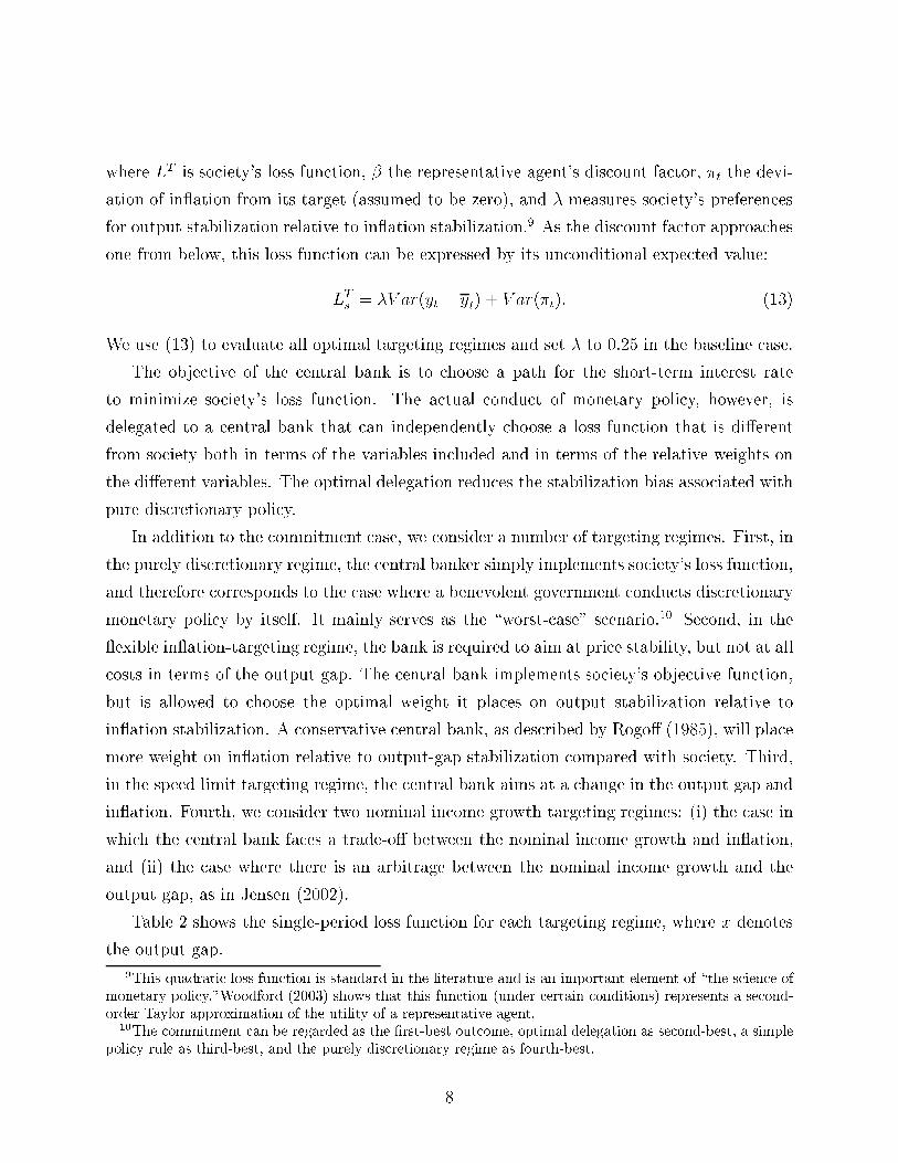
where LT is society's loss function, � the representative agent's discount factor, �t the devi-
ation of in ation from its target (assumed to be zero), and � measures society's preferences
for output stabilization relative to in ation stabilization.9 As the discount factor approaches
one from below, this loss function can be expressed by its unconditional expected value:
LTs = �V ar(yt � yt) + V ar(�t): (13)
We use (13) to evaluate all optimal targeting regimes and set � to 0.25 in the baseline case.
The objective of the central bank is to choose a path for the short-term interest rate
to minimize society's loss function. The actual conduct of monetary policy, however, is
delegated to a central bank that can independently choose a loss function that is di�erent
from society both in terms of the variables included and in terms of the relative weights on
the di�erent variables. The optimal delegation reduces the stabilization bias associated with
pure discretionary policy.
In addition to the commitment case, we consider a number of targeting regimes. First, in
the purely discretionary regime, the central banker simply implements society's loss function,
and therefore corresponds to the case where a benevolent government conducts discretionary
monetary policy by itself. It mainly serves as the \worst-case" scenario.10 Second, in the
exible in ation-targeting regime, the bank is required to aim at price stability, but not at all
costs in terms of the output gap. The central bank implements society's objective function,
but is allowed to choose the optimal weight it places on output stabilization relative to
in ation stabilization. A conservative central bank, as described by Rogo� (1985), will place
more weight on in ation relative to output-gap stabilization compared with society. Third,
in the speed limit targeting regime, the central bank aims at a change in the output gap and
in ation. Fourth, we consider two nominal income growth targeting regimes: (i) the case in
which the central bank faces a trade-o� between the nominal income growth and in ation,
and (ii) the case where there is an arbitrage between the nominal income growth and the
output gap, as in Jensen (2002).
Table 2 shows the single-period loss function for each targeting regime, where x denotes
the output gap.
9This quadratic loss function is standard in the literature and is an important element of \the science ofmonetary policy."Woodford (2003) shows that this function (under certain conditions) represents a second-order Taylor approximation of the utility of a representative agent.
10The commitment can be regarded as the �rst-best outcome, optimal delegation as second-best, a simplepolicy rule as third-best, and the purely discretionary regime as fourth-best.
8

Table 2: Alternative Targeting Regimes
Targeting Regimes Loss functionPrecommitment �2t + �x2tPure discretion �2t + �x2tIn ation targeting (IT) �2t +
b�IT x2tSpeed limit targeting (SLT) �2t +
b�SLT�x2tNominal income growth targeting (NIT1) �2t +
b�NIT1(�t +�yt)2
Nominal income growth targeting (NIT2) �x2t +b�NIT2(�t +�yt)
2
For each and independently of the targeting regime, a grid search is performed to �nd the
optimal value of b�. For example, in ation targeting involves the central bank choosing the
optimal relative weight on x2t . In the case of in ation targeting, depending on its preferences,
the central bank may attach a higher or lower value to in ation compared with society. We
proceed in the same fashion for all the other targeting regimes, each time �nding the optimal
(relative) weight the central bank assigns to its targeting variables.
To evaluate the welfare di�erential between precommitment and the di�erent targeting
regimes, we use two alternative measures as, in Dennis and S�oderstr�om (2002) and Lam
(2003). The �rst measure is the percentage deviation of the optimal targeting regimes from
the precommitment outcome. It is calculated as:
Ldiff = 100[LTR
LC
� 1]; (14)
where LTR and LC are, respectively, the loss-function value under the optimal targeting
regime and precommitment.
Because this measure does not have a direct economic interpretation, we follow Jensen
(2002) and calculate the permanent deviation of in ation from target (the in ation equiva-
lent) when the central bank moves from precommitment to an optimal discretionary regime.
This measure is calculated as:
�diff =p(LTR � LC): (15)
This measure has a more direct economic interpretation, because it indicates how in ation
is a�ected if the central bank chooses to renege on its promises.
9

4 Results
Before evaluating the di�erent targeting regimes, we formally investigate the importance of
lags and the parameter, �; that governs the degree of forward-looking price-setting behaviour
for the size of the stabilization bias.
4.1 The stabilization bias in a model with and without transmis-
sion and information lags
In this section, we compare the dynamic response of the economy following a one-unit cost-
push shock under precommitment and discretion using a model with and without transmis-
sion and information lags. We use the baseline parameters provided in Table 1 to generate
our impulse-response functions.
Figure 1: Impulse-Response Function in the Baseline Hybrid New Keynesian Model
0 10 20 30−20
−15
−10
−5
0
5x 10
−3 (i) Output gap
0 10 20 30−0.005
0
0.005
0.01
0.015
0.02
0.025(ii) CPI
0 10 20 30−0.005
0
0.005
0.01
0.015
0.02
0.025(iii) Nominal interest rate
commitmentdiscretion
Figure 1 shows the response of the economy to a one-period cost-push shock. The unit
cost-push shock leads to an increase in in ation and to a negative output gap under both
discretion and precommitment. To dampen the in ationary pressures, the central bank
10

raises interest rates under both precommitment and discretion. The policy response under
the commitment is, however, less aggressive and more inertial. Under precommitment, the
central bank promises to let the period of in ation be followed by a period of de ation by
creating a more persistent output gap. Since in ation is forward looking, the promise of
a future de ation has a stabilizing role on actual in ation. Consequently, this results in a
more favourable trade-o� between in ation and the output gap.
Under discretion, however, the central bank has no incentive to let the contraction persist
once in ation is back at its target, since the ensuing period of de ation is costly in terms
of welfare. This results in a larger and less inertial policy response and hence in a less
favourable trade-o� between in ation and the output gap.
Figure 2: Impulse-Response Function in the Model with Both Lags
0 10 20 30−12
−10
−8
−6
−4
−2
0
2x 10
−3 (i) Output gap
0 10 20 30−5
0
5
10
15x 10
−3 (ii) CPI
0 10 20 30−5
0
5
10
15
20x 10
−3 (iii) Nominal interest rate
commitmentdiscretion
When the model features transmission and information lags (Figure 2), one striking fea-
ture is that the dynamics of the model under precommitment and discretion are closer, espe-
cially for the output gap. Although the response of the central bank under precommitment
is still more inertial, the interest rate di�erential between precommitment and discretion is
smaller in the model that features lags. Consistent with these smaller di�erences in impulse-
response functions, we �nd that the di�erence between precommitment and discretion|the
stabilization bias|is smaller in the model that features transmission and information lags
11

than in the baseline closed-economy model. Our numerical results con�rm the fact that the
gains from precommitment are e�ectively smaller in the model that includes transmission
and information lags.
4.2 The importance of � for the stabilization bias
Since the size of the stabilization bias depends heavily on the degree of persistence in in-
ation, in this section we show how important the parameter � is for determining the size
of this ineÆciency. We allow for various degrees of forward-looking price-setting behaviour
by varying � between 0 and 1. We expect the stabilization bias to gradually disappear as
� tends to one|as the aggregate supply becomes completely backward-looking|and to be
large when the aggregate supply is forward looking. Figure 3 shows the implications of in-
creasing the importance of backward-looking expectations (the value of �) on the size of the
stabilization bias in all four models. The �rst panel shows the stabilization bias in terms of
percentage deviation, and the second panel displays the permanent increase in in ation.
Figure 3: Size of Stabilization Bias
0 0.1 0.2 0.3 0.4 0.5 0.6 0.7 0.8 0.9 10
5
10
15
20
25
30
35
Coefficient on lagged inflation (φ)
SB
− p
erce
ntag
e de
viat
ion Baseline model
information lagtransmission lagtran and info lag
0 0.1 0.2 0.3 0.4 0.5 0.6 0.7 0.8 0.9 10
0.5
1
1.5
2
Coefficient on lagged inflation (φ)
SB
− in
flatio
n eq
uiva
lent
In all four models, the size of the stabilization bias becomes increasingly smaller as the
12
dynamics becomes increasingly backward looking. In a case where in ation is predomi-
nantly backward looking and expected in ation plays an in�nitesimal role, it should not be
surprising if the stabilization bias disappears.
As expected, the size of the stabilization bias is considerably reduced when the baseline
model is modi�ed to include either a transmission or an information lag. Interestingly, in the
model that features an information lag or both lags, even with forward-looking expectations
in the Phillips curve the gains from commitment remain minuscule. Since the gains from
precommitment are small in the model that features both lags, a targeting regime such as
in ation should perform well, and the need to delegate monetary policy to a central bank
that targets either the change in the output gap or nominal income growth decreases.
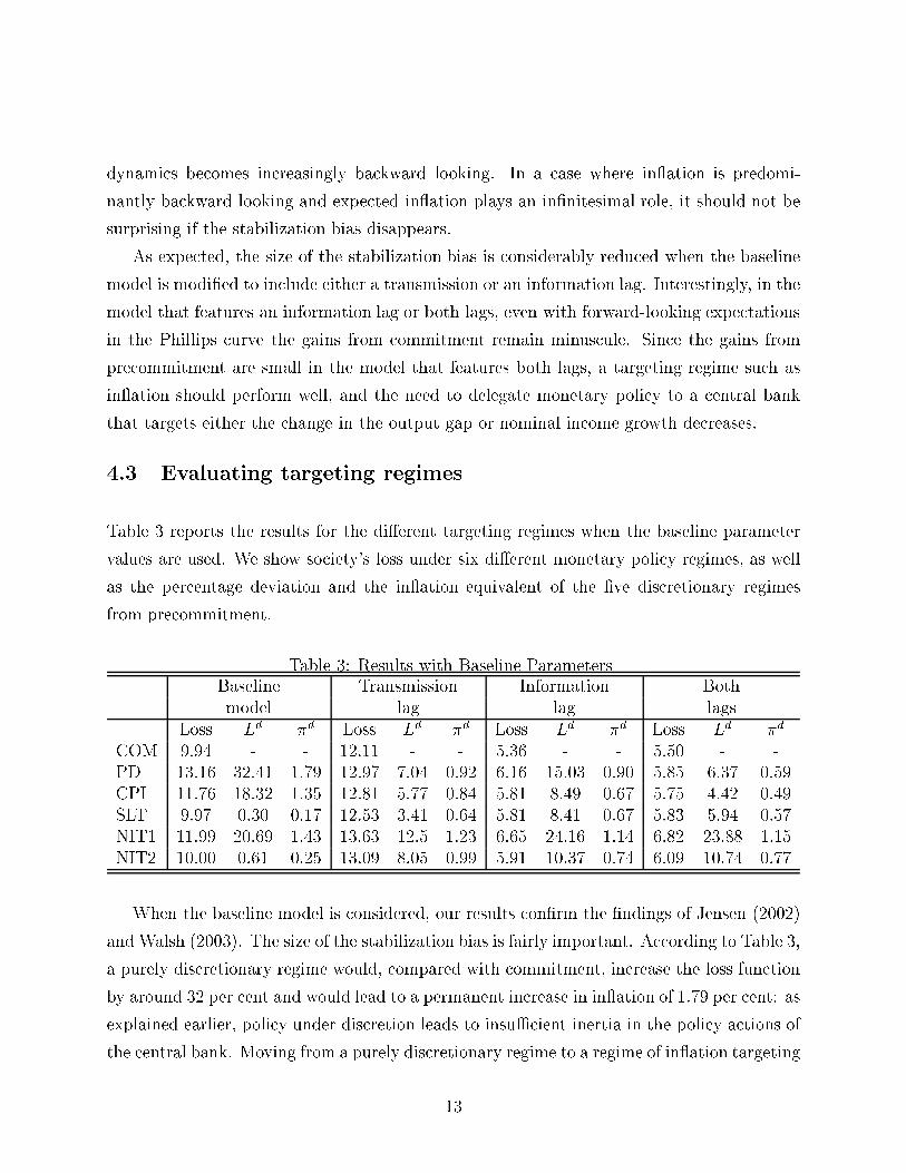
4.3 Evaluating targeting regimes
Table 3 reports the results for the di�erent targeting regimes when the baseline parameter
values are used. We show society's loss under six di�erent monetary policy regimes, as well
as the percentage deviation and the in ation equivalent of the �ve discretionary regimes
from precommitment.
Table 3: Results with Baseline ParametersBaseline Transmission Information Bothmodel lag lag lags
Loss Ld �d Loss Ld �d Loss Ld �d Loss Ld �d
COM 9.94 - - 12.11 - - 5.36 - - 5.50 - -PD 13.16 32.41 1.79 12.97 7.04 0.92 6.16 15.03 0.90 5.85 6.37 0.59CPI 11.76 18.32 1.35 12.81 5.77 0.84 5.81 8.49 0.67 5.75 4.42 0.49SLT 9.97 0.30 0.17 12.53 3.41 0.64 5.81 8.41 0.67 5.83 5.94 0.57NIT1 11.99 20.69 1.43 13.63 12.5 1.23 6.65 24.16 1.14 6.82 23.88 1.15NIT2 10.00 0.61 0.25 13.09 8.05 0.99 5.91 10.37 0.74 6.09 10.74 0.77
When the baseline model is considered, our results con�rm the �ndings of Jensen (2002)
and Walsh (2003). The size of the stabilization bias is fairly important. According to Table 3,
a purely discretionary regime would, compared with commitment, increase the loss function
by around 32 per cent and would lead to a permanent increase in in ation of 1.79 per cent: as
explained earlier, policy under discretion leads to insuÆcient inertia in the policy actions of
the central bank. Moving from a purely discretionary regime to a regime of in ation targeting
13

(with a conservative manner) improves the outcome.11 The welfare gain of adopting in ation
targeting is fairly limited, however, since the deviation from commitment in terms of welfare
remains important.
On the other hand, delegating monetary policy to a central bank that targets the change
in the output gap (SLT) or nominal income growth (NIT2), as in Jensen (2002), results
in large reductions in the loss function. Both targeting regimes, particularly SLT, are able
to replicate the precommitment outcome and are clearly superior to a regime that targets
in ation: as explained in the introduction, they are able to induce inertia in the policy
response of the central bank, thereby acting more in accordance with the outcome under
commitment.
Our results are very di�erent when the baseline model is extended to include transmission
lags and/or information lags. The introduction of a transmission lag into the basic frame-
work considerably reduces the stabilization bias, and thus the need for optimal delegation.
The quantitative gain from commitment in terms of percentage deviation is around 7 per
cent, compared with 32 per cent in the baseline case. Going from pure discretion to in ation
targeting leads to a further reduction in the loss function. The percentage gain from pre-
commitment falls to 5.8 per cent. In this case also, it is optimal to appoint a conservative
central bank.
SLT continues to perform well, but the gains from adopting such a framework relative to
in ation targeting are nevertheless greatly reduced. When we perform a sensitivity test on
the parameter �|which governs the degree of forward-looking behaviour in the aggregate
supply|we �nd that in ation targeting, except for values of � close to the baseline assump-
tion of 0.5, outperforms SLT. There is a marked di�erence between these two regimes as the
aggregate supply function becomes predominantly backward looking (see Table A1 in the
appendix).
The introduction of a transmission lag reduces the bene�ts of precommitment: when
monetary policy a�ects the economy with a lag, policy-makers are less able to make promises
to o�set shocks, thereby reducing the eÆcacy of credible commitments. Moreover, in a
framework that has transmission (and information) lags, the central bank can no longer
perfectly insulate the economy from demand shocks. Since precommitment is especially
valuable in improving the trade-o� between in ation and the output gap when the economy
11The optimal � is 0.15, lower than the value that society assigns to output stabilization.
14

is hit with shocks that create a trade-o� for society, such as a cost-push shock. On the other
hand, when shocks such as demand and technology|that pose no trade-o� for society|
become increasingly important, as in the framework with transmission lags, the need for
precommitment is greatly reduced.
This also explains why delegating monetary policy to a central bank that targets nominal
income growth (or the change in the output gap) becomes less attractive. A downside of
NIT2 is that it is not very eÆcient in dealing with shocks that pose no trade-o� to society.
Since the central bank cannot perfectly insulate the economy from demand shocks when a
transmission lag is introduced, this makes a regime of NIT growth less attractive. In Tables
A1 and A2 in the appendix, we �nd that in ation targeting outperforms NIT2 even for very
forward-looking speci�cations of the aggregate supply.
When an information lag is introduced into the baseline model, it leads to a reduction in
the welfare gain from precommitment. In this variant of the baseline model, SLT continues to
perform well. However, the di�erence between this regime and a regime that targets in ation
is minuscule. For example, the quantitative di�erence between the two regimes in terms of
loss function is less than 0.1 per cent. As in the framework that features a transmission lag
only, this result is not robust when we allow for di�erent degrees of forward-lookingness in
the aggregate supply function. As we show in Table A2 of the appendix, in ation targeting
is more eÆcient than SLT for various parameter con�gurations.
One of the main advantages of commitment is its ability to appropriately a�ect private
agents' expectations and hence their current expenditure decisions. However, if expectations
are predetermined and the actions of the central bank are not forecastable in advance, then
this limits the ability of the central bank to in uence the decisions and expectations of private
agents, since agents cannot incorporate the latest policy decisions of the central bank in their
decision-making process. As a result, the need for credible promises becomes less important.
The model that combines transmission and information lags further reduces the welfare
gain from precommitment. This result is not surprising, because the e�ects of a transmis-
sion lag and an information lag reinforce each other, for reasons described earlier. The
impulse-response function (Figure 2), which we discussed in section 4.1, con�rms that the
optimal response under precommitment and discretion is not very di�erent. It is interesting
that, in this model, the purely discretionary case is very close to a regime that targets the
change in the output gap, and it does better than both nominal income targeting regimes.
Dennis and S�oderstr�om (2002) obtain a similar result when they use the model of Rude-
15

busch (2002), which is structurally similar to our simple model. In fact, they obtain an
even stronger result|there is practically no di�erence between precommitment and discre-
tion in the Rudebusch (2002) framework|since the Rudebusch model embodies even more
backward-looking pricing behaviour.
Even more interesting is the performance of in ation targeting relative to SLT and NIT2
in this model.12 Our �ndings reveal that in ation targeting performs particularly well under
various parameter con�gurations (see Tables A1 and A2 in the appendix). The only case
in which in ation targeting does not perform well is when more persistence is introduced
into the process for the cost-push shock. Although in ation targeting requires an even more
conservative central banker, the case for SLT and NIT2 relative to in ation targeting is
reinforced when the parameter e is increased to 0.7. This result is not surprising, since the
importance of precommitment to future contractions is enhanced when the shock to in ation
becomes persistent.13
Apart from this parameter con�guration, in ation targeting as a delegation scheme would
be optimal. This result is robust and is very di�erent from results obtained using the baseline
model. In the baseline model, in ation targeting, except when in ation expectations are
predominantly backward looking, is inferior to SLT and NIT2 under di�erent parameter
speci�cations (see Table A2). Figures 4 and 5 show the performance of SLT and NIT2
relative to in ation targeting. As stated earlier, except when in ation is predominantly
backward looking, SLT and NIT2 are superior to in ation targeting in the baseline model.
On the other hand, in the model with transmission and information lags, in ation targeting,
irrespective of the degree of forward-looking pricing behaviour, outperforms both SLT and
NIT2.
12When baseline parameter values are used, we �nd that targeting in ation amounts to appointing aconservative central bank, since the optimal value of � is 0.15.
13This result is very robust across all models. It is somewhat of a paradox that in ation targeting becomesincreasingly inferior the more persistent the e�ects of the shocks to in ation.
16

Figure 4: Loss Relative to In ation Targeting in the Baseline Model
0 0.1 0.2 0.3 0.4 0.5 0.6 0.7 0.8 0.9 1−20
−15
−10
−5
0
5
10
15
20
Coefficient on lagged inflation (φ)
Per
cent
age
devi
atio
n fr
om lo
ss fu
nctio
n un
der
CP
ISLTNIT2
Figure 5: Loss Relative to In ation Targeting in Models with Both Lags
0 0.1 0.2 0.3 0.4 0.5 0.6 0.7 0.8 0.9 10
5
10
15
20
25
Coefficient on lagged inflation (φ)
Per
cent
age
devi
atio
n fr
om lo
ss fu
nctio
n un
der
CP
I
SLTNIT2
17

5 Concluding Remarks
Using an otherwise conventional New Keynesian framework augmented with transmission
and information lags, we have shown that the stabilization bias and optimal monetary policy
delegation can be quite di�erent. We have found that, in a model with predetermined
expenditure and lags in the transmission mechanism, the size of the stabilization bias|the
ineÆciency inherent in discretionary policy-making|is greatly reduced. The common belief
among central bankers is that monetary policy a�ects the economy with a lag. Moreover,
if agents' consumption and investment decisions are largely predetermined, the stabilization
bias may not be very severe after all. Obviously, this issue deserves further research.
Moreover, optimal delegation in such a framework amounts to targeting in ation in a
conservative manner. This result is very di�erent from those obtained using a conventional
New Keynesian sticky-price model. In such a framework, in ation targeting is inferior to a
regime that targets either the change in the output gap or nominal income growth.
With transmission and information lags added to the model, precommitting to a given
policy becomes less important, because policy-makers are less able to credibly o�set and pre-
empt shocks, even if their promises are fully credible. On the other hand, with information
lags added to the model, private agents cannot incorporate the most recent decisions by
policy-makers and hence its likely impact on future economic outcomes. Under both cases,
the expectations channel and hence precommitment becomes less important.
18

Bibliography
Barro, R.J. and D.B. Gordon. 1983. \Rules, Discretion and Reputation in a Model of
Monetary Policy." Journal of Monetary Economics 12(1): 101{22.
Blinder, A.S. 1998. Central Banking in Theory and Practice. Cambridge: MIT Press.
Calvo, G. 1983. \Staggered Prices in a Utility-Maximizing Framework." Journal of Mone-
tary Economics 12: 383{98.
Christiano, L.J., M.S. Eichenbaum, and C.L. Evans. 2004. \Nominal Rigidities and the
Dynamic E�ects of a Shock to Monetary Policy." Journal of Political Economy. Forth-
coming.
Clarida, R., J. Gal��, and M. Gertler. 1999. \The Science of Monetary Policy: A New
Keynesian Perspective." Journal of Economic Literature 37: 1661{1707.
Dennis, R. and U. S�oderstr�om. 2002. \How Important is Precommitment for Monetary
Policy?" Sveriges Riksbank Working Paper No. 139.
Friedman, M. 1968. \The Lag in E�ect of Monetary Policy." Journal of Political Economy
69: 447{66.
Fuhrer, J. and G. Moore. 1995. \In ation Persistence." Quarterly Journal of Economics
CX: 127{60.
Jensen, H. 2002. \Targeting Nominal Income Growth or In ation?" American Economic
Review 4: 928{56.
Kydland, F.E. and E.C. Prescott. 1977. \Rules Rather Than Discretion: The Inconsistency
of Optimal Plans." Journal of Political Economy 85: 473{91.
Lam, J-P. 2003. \Alternative Targeting Regimes, Transmission Lags, and the Exchange
Rate Channel." Bank of Canada Working Paper No. 2003-39.
Roberts, J. 1995. \New Keynesian Economics and the Phillips Curve." Journal of Money,
Credit and Banking 27(4): 975{84.
19
Rogo�, K. 1985. \The Optimal Degree of Commitment to an Intermediate Monetary
Target." Quarterly Journal of Economics 100: 1169{89.
Rotemberg, J.J. and M. Woodford. 1999. \Interest Rate Rules in an Estimated Sticky
Price Model." In Monetary Policy Rules, edited by J. Taylor. Chicago: University of
Chicago Press.
Rudebusch, G. 2002. \Assessing Nominal Income Rules for Monetary Policy with Model
and Data Uncertainty." Economic Journal 112: 402{32.
Rudebusch, G. and L.E.O. Svensson. 1999. \Policy Rules for In ation Targeting." In
Monetary Policy Rules, edited by J. Taylor. Chicago: University of Chicago Press.
Smets, F. and R. Wouters. 2003. \An Estimated Stochastic Dynamic General Equilibrium
Model of the Euro Area." Journal of European Economic Association 1(5): 1123-75.
S�oderlind, P. 1999. \Solution and Estimation of RE Macromodels with Optimal Policy."
European Economic Review 41: 1111{46.
S�oderstr�om, U. 2001. \Targeting In ation with a Prominent Role for Money." Sveriges
Riksbank Working Paper No. 123.
Vestin, D. 2000. \Price-Level Targeting vs. In ation Targeting in a Forward-Looking
Model." IIES Stockholm University Working Paper.
Walsh, C.E. 1985. \Optimal Contracts for Independent Central Bankers." American Eco-
nomic Review 85(1): 150{67.
|||. 2003. \Speed Limit Policies: The Output Gap and Optimal Monetary Policy."
American Economic Review 93(1): 265{78.
Woodford, M. 2003. Interest & Prices. Princeton: Princeton University Press.
20

Appendix A: Sensitivity Test Results
Table A1: Results with � = [0:01; 0:1; :::; 0:99]
� Disc CPI SLT NIT1 NIT2Ldiff �diff Ldiff �diff Ldiff �diff Ldiff �diff Ldiff �diff
0.01 8.55 0.42 8.55 0.42 2.86 0.25 34.70 0.85 7.99 0.410.1 10.35 0.51 10.35 0.51 3.07 0.28 33.37 0.91 8.85 0.470.2 13.66 0.66 13.48 0.65 3.30 0.32 31.47 1.00 8.97 0.530.3 19.76 0.92 18.53 0.89 3.31 0.38 28.56 1.11 7.29 0.560.4 30.05 1.38 24.01 1.24 2.42 0.39 24.11 1.24 3.58 0.480.5 32.41 1.80 18.32 1.35 0.30 0.1712 20.69 1.43 0.61 0.250.6 19.32 1.67 8.49 1.11 1.23 0.42 29.17 2.04 2.93 0.650.7 8.83 1.26 2.83 0.71 6.51 1.08 49.82 2.98 5.65 1.000.8 3.43 0.83 0.08 0.40 12.28 1.56 73.03 3.81 6.52 1.140.9 0.94 0.44 0.06 0.11 16.65 1.87 94.43 4.45 6.62 1.180.99 0.05 0.11 0.05 0.11 19.38 2.04 111.51 4.89 6.46 1.18
Baseline Model
Table A1: Results with � = [0:01; :::; 0:99]
� Disc CPI SLT NIT1 NIT2Ldiff �diff Ldiff �diff Ldiff �diff Ldiff �diff Ldiff �diff
0.01 5.29 0.38 5.29 0.38 18.29 0.71 27.10 0.86 6.61 0.430.1 6.30 0.45 6.30 0.45 15.78 0.71 21.74 0.83 8.03 0.510.2 7.86 0.56 7.82 0.55 13.06 0.72 16.64 0.81 10.86 0.650.3 9.82 0.71 9.54 0.70 10.13 0.72 12.60 0.81 12.11 0.790.4 10.74 0.90 9.90 0.86 6.70 0.71 10.00 0.87 9.01 0.830.5 7.04 0.92 5.77 0.84 3.41 0.64 12.50 1.23 8.05 0.990.6 2.01 0.61 1.18 0.46 5.35 0.99 29.34 2.31 10.99 1.410.7 0.30 0.27 0.14 0.18 11.33 1.61 53.45 3.50 10.77 1.570.8 0.05 0.11 0.05 0.11 15.84 2.01 73.24 4.32 9.07 1.520.9 0.00 0.04 0.00 0.04 18.79 2.23 89.53 4.87 7.67 1.430.99 0.00 0.01 0.00 0.01 20.93 2.36 102.84 5.23 6.79 1.34
Transmission Lag
21
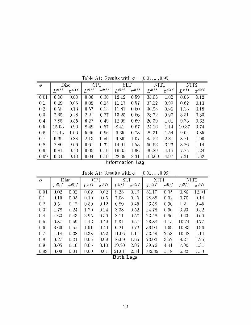
Table A1: Results with � = [0:01; :::; 0:99]
� Disc CPI SLT NIT1 NIT2Ldiff �diff Ldiff �diff Ldiff �diff Ldiff �diff Ldiff �diff
0.01 0.00 0.00 0.00 0.00 12.12 0.59 35.93 1.02 0.05 0.120.1 0.09 0.05 0.09 0.05 11.17 0.57 33.52 0.99 0.62 0.130.2 0.58 0.13 0.57 0.13 11.81 0.60 30.98 0.96 1.13 0.180.3 2.35 0.28 2.21 0.27 13.25 0.66 28.72 0.97 3.31 0.330.4 7.85 0.55 6.27 0.49 12.09 0.69 26.39 1.01 9.73 0.620.5 15.03 0.90 8.49 0.67 8.41 0.67 24.16 1.14 10.37 0.740.6 12.42 1.00 5.46 0.66 6.65 0.73 29.31 1.54 9.04 0.850.7 6.65 0.88 2.13 0.50 9.86 1.07 45.82 2.31 8.71 1.000.8 2.80 0.66 0.67 0.32 14.91 1.53 66.63 3.23 8.26 1.140.9 0.81 0.40 0.05 0.10 19.35 1.96 86.89 4.15 7.75 1.240.99 0.04 0.10 0.04 0.10 22.39 2.31 103.60 4.97 7.31 1.32
Information Lag
Table A1: Results with � = [0:01; :::; 0:99]
� Disc CPI SLT NIT1 NIT2Ldiff �diff Ldiff �diff Ldiff �diff Ldiff �diff Ldiff �diff
0.01 0.02 0.02 0.02 0.02 8.23 0.49 31.17 0.95 0.60 12.940.1 0.10 0.05 0.10 0.05 7.08 0.45 28.88 0.92 0.70 0.140.2 0.51 0.12 0.50 0.12 6.80 0.45 26.58 0.90 1.21 0.450.3 1.78 0.24 1.70 0.24 8.38 0.52 24.78 0.90 3.23 0.320.4 4.63 0.43 3.95 0.39 8.11 0.57 23.48 0.96 9.23 0.600.5 6.37 0.59 4.42 0.49 5.94 0.57 23.88 1.15 10.74 0.770.6 3.60 0.55 1.91 0.40 6.21 0.72 33.90 1.69 10.83 0.960.7 1.14 0.38 0.38 0.22 11.06 1.17 53.49 2.58 10.48 1.140.8 0.27 0.21 0.05 0.09 16.09 1.65 73.02 3.52 9.27 1.250.9 0.05 0.10 0.05 0.10 19.30 2.05 89.76 4.41 7.90 1.310.99 0.00 0.01 0.00 0.01 21.01 2.34 102.89 5.18 6.82 1.33
Both Lags
22

Table A2: Results with Di�erent Values for ��y, � and e
Regimes ��y = 0:01 � = 0:01 � = 0:2 e = 0:3 e = 0:7Ldiff �diff Ldiff �diff Ldiff �diff Ldiff �diff Ldiff �diff
Disc 32.41 1.79 33.79 2.88 17.64 0.77 44.04 3.37 78.97 11.56CPI 18.32 1.35 14.58 1.89 14.85 0.71 21.16 2.34 21.52 6.03SLT 0.30 0.17 0.25 0.14 0.40 0.11 0.40 0.31 0.26 0.67NIT1 23.10 1.51 103.62 5.05 5.77 0.44 17.52 2.13 9.57 4.02NIT2 2.44 0.49 2.94 0.85 10.48 0.59 0.62 0.40 2.72 2.14
Baseline Model
Regimes ��y = 0:01 � = 0:01 � = 0:2 e = 0:3 e = 0:7Ldiff �diff Ldiff �diff Ldiff �diff Ldiff �diff Ldiff �diff
Disc 6.94 0.92 12.38 1.78 3.75 0.52 9.26 1.69 14.42 5.28CPI 5.69 0.84 7.16 1.36 3.75 0.52 7.27 1.50 8.38 4.03SLT 4.01 0.70 5.56 1.20 2.32 0.41 2.57 0.89 13.09 5.03NIT1 13.83 1.31 64.36 4.07 10.12 0.85 13.42 2.03 8.94 4.16NIT2 9.60 1.09 3.02 0.88 21.48 1.24 6.13 1.37 2.72 2.14
Transmission Lag
Regimes ��y = 0:01 � = 0:01 � = 0:2 e = 0:3 e = 0:7Ldiff �diff Ldiff �diff Ldiff �diff Ldiff �diff Ldiff �diff
Disc 14.52 0.90 23.05 1.44 3.98 0.38 23.81 1.35 75.09 8.14CPI 8.20 0.67 9.94 0.95 3.35 0.35 12.33 0.97 21.19 4.32SLT 10.23 0.75 15.34 1.18 3.70 0.37 6.48 0.71 0.97 0.92NIT1 27.39 1.23 85.96 2.79 16.47 0.78 22.06 1.30 10.41 3.03NIT2 12.34 0.83 7.77 0.84 17.77 0.81 8.41 0.80 3.54 1.77
Information Lag
Regimes ��y = 0:01 � = 0:01 � = 0:2 e = 0:3 e = 0:7Ldiff �diff Ldiff �diff Ldiff �diff Ldiff �diff Ldiff �diff
Disc 6.17 0.59 13.51 1.11 1.92 0.288 9.80 0.88 27.60 5.01CPI 4.28 0.49 6.53 0.77 1.82 0.27 6.54 0.72 12.20 3.33SLT 7.12 0.64 13.70 1.11 1.60 0.26 4.91 0.62 1.23 1.06NIT1 26.66 1.24 82.40 2.73 16.61 0.83 23.28 1.36 15.79 3.79NIT2 12.76 0.85 6.60 0.77 21.45 0.95 9.38 0.86 8.69 2.81
Both Lags
23


Bank of Canada Working PapersDocuments de travail de la Banque du Canada
Working papers are generally published in the language of the author, with an abstract in both officiallanguages.Les documents de travail sont publiés généralement dans la langue utilisée par les auteurs; ils sontcependant précédés d’un résumé bilingue.
Copies and a complete list of working papers are available from:Pour obtenir des exemplaires et une liste complète des documents de travail, prière de s’adresser à:
Publications Distribution, Bank of Canada Diffusion des publications, Banque du Canada234 Wellington Street, Ottawa, Ontario K1A 0G9 234, rue Wellington, Ottawa (Ontario) K1A 0G9E-mail: [email protected] Adresse électronique : [email protected] site: http://www.bankofcanada.ca Site Web : http://www.banqueducanada.ca
20042004-36 Optimal Taylor Rules in an Estimated Model of
a Small Open Economy S. Ambler, A. Dib, and N. Rebei
2004-35 The U.S. New Keynesian Phillips Curve: AnEmpirical Assessment A. Guay and F. Pelgrin
2004-34 Market Valuation and Risk Assessment ofCanadian Banks Y. Liu, E. Papakirykos, and M. Yuan
2004-33 Counterfeiting: A Canadian Perspective J. Chant
2004-32 Investment, Private Information, and Social Learning: ACase Study of the Semiconductor Industry R. Cunningham
2004-31 The New Keynesian Hybrid Phillips Curve: An Assessmentof Competing Specifications for the United States D. Dupuis
2004-30 The New Basel Capital Accord and the CyclicalBehaviour of Bank Capital M. Illing and G. Paulin
2004-29 Uninsurable Investment Risks C. Meh and V. Quadrini
2004-28 Monetary and Fiscal Policies in Canada: Some InterestingPrinciples for EMU? V. Traclet
2004-27 Financial Market Imperfection, Overinvestment,and Speculative Precaution C. Calmès
2004-26 Regulatory Changes and Financial Structure: TheCase of Canada C. Calmès
2004-25 Money Demand and Economic Uncertainty J. Atta-Mensah
2004-24 Competition in Banking: A Review of the Literature C.A. Northcott
2004-23 Convergence of Government Bond Yields in the Euro Zone:The Role of Policy Harmonization D. Côté and C. Graham
2004-22 Financial Conditions Indexes for Canada C. Gauthier, C. Graham, and Y. Liu
2004-21 Exchange Rate Pass-Through and the Inflation Environmentin Industrialized Countries: An Empirical Investigation J. Bailliu and E. Fujii