The implementation of clean production and the use of ... · PDF fileThe implementation of clean production and the use of neural networks in forecasting waste management ... 2. the

The implementation of clean production and the use of neural networks in forecasting waste management

VALERIU LUPU1, CATALIN LUPU2, NICOLAE MORARIU3

Faculty of Economics and Public Administration “Stefan cel Mare” University of Suceava

13, Universitatii str., Suceava ROMANIA

[email protected] ,[email protected], [email protected] http://www.multibiometrics.ro/

Abstract: In this article we present: the implementation of "clean production" which means production based on careful

evaluation of the product since its design phase to ensure that both the product and processes related to it at all stages of its life cycle (ranging the extraction of raw materials, manufacturing, packaging, consumer / use, waste collection and treatment) promotes the interests of the community, in particular as regards the environment.

Clean production has four main elements: - Caution, which involves taking measures insurers even in the case of yet unconfirmed suspicions concerning a potential nocivitate to human health or the environment; - Prevention, as expression of conscience that is cheaper and more efficient to prevent environmental degradation than to provide remedies; - Democratic participation in decision-making of all stakeholders - An integrated and holistic approach.

a new concept taking in consideration the sweepings administration and which consist in:

1. the employment of neuronal network for predict serial time representing sweepings amount which are collected from population in time. The problems of prediction the serial time can be associated with neuronal network call “feed-forward”. Number of entrances unities are equal than number of emergences unities. The number of emergences unities represents the target of prediction. The prediction “one step before” can be realized with an emergences unities network, and the prediction with “K steps before” can be associate to a network with K emergences unities.

Examples: 1. A model of a neuronal network “one step before”, which use six terms of

serial time to predict the next term of series ( 6 neurons at entrance, 15 in hide tier and one in emergence tier, entering ==(xt-1, xt-2, xt-3, xt-4, xt-5, xt-6, ), emergence = xt );

2. A model of a neuronal network in to 8 terms of serial time are using for predict the next 2 terms;

3. A model of neuronal network in to 6+2(t-1) terms of serial time are using for predict the next “t” terms.

the employment of a new index BPL for the prognosis of sweepings administration consulting of:

1. population (the index of variety of population); 2.“the habitat” of sanitation services; 3. economic development:

the economic development with α% / year represents an increase of assimilated sweepings amount emanated from shop keeping (Pce – the economic development percent );

the grows with β% / year of purchase represent an increase of sweepings (Pv –

WSEAS TRANSACTIONS on SYSTEMS and CONTROL

VALERIU LUPU,CATALIN LUPU,NICOLAE MORARIU

ISSN: 1991-8763 722 Issue 9, Volume 3, September 2008

the purchase grows percent) 4. the amount of sweepings collected from population and economics agents; 5. the amount of sweeping from gardens, plaza and streets; 6. the amount of mud from service station, from buildings and knockings. For prognosis of sweepings administration development for a certain region and for a certain period of time, are used the scripts. For certain period are constituted the purposes and aims for short , medium and long time. Each script must have the same base which includes the historical evolution of generation system of sweepings for a period between 5 and 7 years. Inside of scripts are constituted the alternatives. Each alternative describe an integrated system of management of sweepings which includes the available and practical operating method of recycle, treatment and elimination of sweepings.

The main criterions of selection for the best script have to accomplish the principles of permanent development:

- to have minimal negative effects about environment;

- to be permissible in socially; - to be doable in economically.

Key-Words: neural network, sweeping administration, prognosis, economic development, serial time.

1. Brainy prognosis systems used for sweepings administration 1.1. The importance of prognosis systems

used for sweepings administration. Prognosis systems of sweepings administration are able to stock real information, about some events and evolutions that can appearance in the future. The problem of sweepings administration is at present and each country must have a solution as regards number and proportion of cesspits. Sweepings administration, an important composition of an environment strategy, is relegating at collecting, transportation, treatment and elimination sweepings activities. In last decades more and more efforts are pointed in looking the best solution for stopping global pollution. For that were created the commissions for preventing pollution, governmental and non-governmental organisms for solving this problem partially at least, as regards variety and continuity of technologies [1]. The information technology and superficial brainy can play a very important role in getting over some impediments which appearance in tentative to prevent and stop pollution. Thus, in case of preventing or decreasing pollution we can find some IT actions steps:

2. the realization of some coherent informational substructure, intended to stock up the information (e.g. database of pollution premonition measures);

3. the realization of some applications which can find the real answer at some problems which can’t be solved without IT programs

help(e.g. furnaces used for the cremation of sweepings);

4. other types of applications, such as: *communication modules between different organisms interested in premonition pollution;

*children games whom subject is pollution in this way we can assure a good education of young people;

5. the employment of neuronal networks for prognosis of

sweepings administration using time serial;

The “pollution premonition” is a term used in USA and in Europe is used the term of “Cleaner Production” (PC). PC is a preventive onset of environment management. This concept is called also eco-efficacy, pollution premonition or green outputs [2]. PC is referring on modality of proprietary and services production without impact about environment, using the present technology and economy. PC doesn’t limit the development, this one insists in order that development must be ecological. PC must not be looked only like an environment strategy, because it takes in consideration also the economic aspect. In PC context, the sweepings are treaty like an “output” which has negative economic value. Whatever activities which intend to reduce the input of raw materials and energy, or intend to prevent or to reduce the sweepings can make the productivity

WSEAS TRANSACTIONS on SYSTEMS and CONTROL VALERIU LUPU,CATALIN LUPU,NICOLAE MORARIU


to grow up and can bring financial profit. Like “win-win” strategy, PC protects the environment, consumer and worker in the same time with increase of industrial efficacies, profitability and competitive. 1.2. The application of clean output PC can be applying in many ways: 1.2.1 Overheads measures: the taking of measures at managerial and operational level for preventing: - drippings - trickles 1.2.2 The substitute of raw materials

• raw materials which are not so toxic (the substitute of whitening factors with chlorine)

• recycling materials (are : Sun, water, air, wood, the animals, etc.)

• materials which has a long existence. 1.2.3. The efficacy control of process: the check of

process for making this efficient by reduction of sweepings and transmitter , the modification of :

• operation processes ; • working instruction ;

1.2.4. The optimize of installations : the modification of installation for :

• the efficiency increase of production process;

• the decreasing of sweepings and pollution transmitters production;

1.2.5. The change of technology: for reduction of sweepings and transmitters production during process:

• the change of technology; • the change of some technologic sequences.

1.2.6. The recycling on-site: • the definition of sweepings; • the decreasing of blocking demand and of

treatment and storage price. 1.2.7. The production of secondary outputs: the

conversion of sweepings in secondary outputs, which can be used as raw materials .

1.2.8. The output modification: the modification of output characteristics for:

• the decrease of medium impacts of output during its life;

• the decrease of medium impacts of production process.

1.3. The enterprise strategy The strategy of an enterprise is the outline which defines:

• the enterprise purpose; • the strategies which one the enterprise

will follow it; • the necessary resorts; • the responsibilities;

The strategy is an ensemble of analytic methods used for understanding and increasing of enterprise position as regards the free trade zone. It makes the relationship between internal capability of enterprise and external condition of it [3]. The "liniation" of strategy will follow the mains tree levels:

1. operational strategy – which forecast the implementation methods of capital goods used by enterprise.

2. deal strategy – the methods of competitively maintenance and the win of new free trade zone ring;

3. enterprise strategy – ensemble of internal and external measures.

The competitively requests are; • technique capacities; • financial capacity.

The advantage of competitively win are; 1. tangibles elements : licensees, monopoly,

etc 2. intangibles elements: the best managers,

teamwork, etc. PC is a world movement at par acceded a lot of trusts. The Pc method implementation makes good technical and financial enterprise performances. Actually techniques and concepts stand up of a new scientifique strategy, representing a big contribution at reach of objectives and resolving the environment protection problem. As strategy of environment performances increase, PC is situated successfully in competitive enterprise strategy. 1.4 The implement of “cleaner poduction” PC means any which activity reduces the amont of losse produced in a commercial his enterprise.PC an administration a residues, not being his dismission doctor it a residues after these were already in a generate enterprise the loss can be:

• Boat sauf aze wagons flowed unobserved from his pipelines vessels;

• The used useless energy to the of a remaking excessive amounts of his steams warm water, necessary the technological his process of the needs of the enterprise;

• The used-up unadvisable waters in a the system of defecation overachiever;

• Rows materials, materials and produced finite or which semifinite depreciated pursuant using , manipulation, storage.

PC or the minimization of loss is achieved through the of a development the systematic



program of missed bare the possible solutions of the adhibition the best one maul solution [4]. Because the project of PC comprises the determination and the of a pursuit big number of loss and which emissions comes from an important number of sources , the program of implementation is complex. He is due to enjoied the support of management ,except than how much commitment and as the support continuously. A good program prompts, also the how much implication the much maul peoples and the systematic gave the informations and the evaluation expeditures.

Therebefore PC prompts: • Employ the manager; • The implication of the camera – mans; • The onset organized.

The requirements for a team of PC are: • Equip is able to identify the timeliness, to develop solutions and implement them; • The size and his components is thus choosed that to present functions different interests.

A successful program needs an which chiefs has the authority took in a decisions good organized programs, each person from firm gambles really a role in put in practices a solutions, identifying the loss and developing solutions foe their minimization, the program becoming an usual activity the motivated popularly the wage earner enterprises[5]. Figure 1 is represented the strategy continue PC:

Fig. 1 The strategy of continue PC A program of PC difficult when is good organized, the tasks are rigorous delivered and followed. Specify as the minimization of the loss isn't equivalent to the auditing programs of pollution, such as the treatment of residual his waters of the removal of the residues [6]. The clean production is achieved through three logical steps:

1. the inventory of the sources – waves are

generated the residues and the emissions? 2. the evaluation of the causa – why are

generated the residues and emissions? 3. the generation of the opinion – how can be

eliminated these causes? The evaluation of clean production is achieved the next in steps: Start Phase 1. Peparation 1.1 Constitute equip PC 1.2 Print phases process

• Is specified all the process, inclusively production handle and the material transport, utilities;

• Heeded special the occasional operations(wash the ablution, etc)

• Is identified – the most important – the entrances and come out: materials, energy, water, residues, emissions;

1.3 Objectives selection for estimate PC. • Economic considerations – loss of money

and composition of the fluxes of residues; • Considerations of average – the volume and

the composition of the fluxes of residues; • Technical considerations – the potentials of

improvement AnalysesPhase 2. Analyse the phases of process 1. preparation diagram flux

• "material balance- sheet the power (on basis of binds the preservation of table: materials entered + materials produced = materials comed + spent materials);

Arrogation costs: • the produced intermediaries, operatic

costs, costs of collection handle the residues;

• External costs: taxes for avacuations; • Panality costs for settlement. Analyse the causes which produce sweepings

• The impact of features produced; • The impact of technical facors –

process, equipments, mountings the equipments, pipelines, systems of monitorising;

• The impact of practices operatic – planning production, procedures operatic, programs of enterprise, instruct the personnel;

• The impact of handle, transports residues.

Phase 3. Generation timeliness PC • Develop the timeliness PC

i. the encouragement of the through innovative , solicit of ideation outwardy the



team (the encouragement all ones employee participation of the enterprise).

ii. Examination of manual databases, pervious reports PC, bench markinr of technologists;

iii. Is verified all the preventive practices: modification of produced , the change of raw materials, the change of the technology , the modification of the equipments, the improvement check of the process, local recovery , good management, generation of useful products.

Selection timeliness employable PC: iv. the implementation of obvious feasible

options; v. the rejection of insubstantial options.

The improvement Phase 4. Selection timeliness PC The evaluation of remained options:

I. the technical evaluation: the availability and the confidence equipment; requirements for upkeep; technical necessary capacity(camera-mans, technicians);

II. the financial evaluation: investments(equipments, buildings, operate), costs and benefits operatic; economic calculi (miss of amortization);

III. evaluation from the viewpoint of appearances of average: reduce the amount of pollutions; reduce the toxicity of pollutions; reduce the consumption of material, reduce the consumption of energy, reduce the solution of implantation combination of the results, technical evaluation, economic evaluation of average.

Phase 5. Implementation of PC solutions 1. the preparation of the plan of the

implementation; 2. execution implement PC 3. monitorizaring and evaluation results,

comparison the results obtained with one preconisating

Integrate Phase 6. Support solutions PC 4. the definiteness of organizational structure

for PC; 5. the implication of all employees through

training and benefits; 6. the elaboration of politics and the strategy

long term PC; 7. the integration PC in the technical

development the integration of the concept of the resa

8. earch of technological development, in curricula the schoolboy.

An important role a material to a these objective solution of PC constitute the bookkeeping for the manangement environment (environment

management accounting= EMA). EMA is can defined as : the identification , the collection , the estimation , the material use of the informations concerning the costs of average, and other informations of costs, incite for the taking of how much decisions of the average from the frame organizations. Utilizations and advantages of EMA(from site). 2. Modern systems of used-up forecast for the administration residues The system of flag and warning have a special case of the general informational systems and communicational system from a firm. Their role is those to delivered informations on strength of gived existences about an events and what evolutions can appear in the future, as for example the ecologic hollows for the sockage residues next in years. Of a such importance systems, follows when in the current activity of the firm appear negative events which effects are can counteracted through which measures taken the in temporally useful. Is can said as the systems of warming and forecast am which systems generates "for acts" and which I improve the performances of the managers through which I improve the performances of the managers through cognition and anticipation [7]. These systems of forecast some closed systems, which in nobody can't realize what is going on, on the contrary, they open systems, transparencies, waves are can see all the relations and the structural connections between the which elements underline the forecasts elaborate. Therefore, the systems of forecast don't help merely earlier warning about what events can appear, they represent an instrument of proper thing, what which the engaged firms works the determination and the pursuit of the relations respective cause of the consequences of the activity and the decisions on which take them. Still from these implementation systems the users are accustomed to the intimation of structural relations of causal si among undertake and average her external and the internal. This is the kind and their shares shall become transparencies as apprehended the elements of average which influences the activity of the firm [8]. A system of forecast and warning can be described in a form simplify as follows:



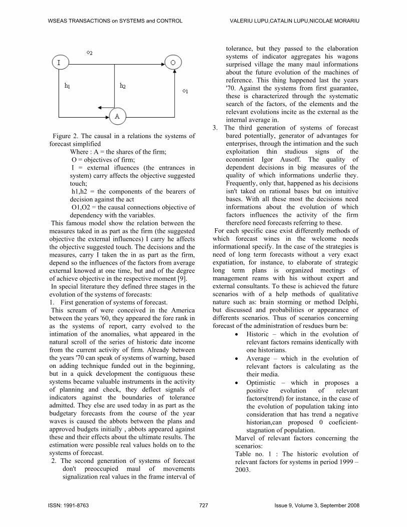
Figure 2. The causal in a relations the systems of forecast simplified

Where : A = the shares of the firm; O = objectives of firm; I = external ifluences (the entrances in system) carry affects the objective suggested touch; h1,h2 = the components of the bearers of decision against the act O1,O2 = the causal connections objective of dependency with the variables.

This famous model show the relation between the measures taked in as part as the firm (the suggested objective the external influences) I carry he affects the objective suggested touch. The decisions and the measures, carry I taken the in as part as the firm, depend so the influences of the factors from average external knowed at one time, but and of the degree of achieve objective in the respective moment [9]. In special literature they defined three stages in the evolution of the systems of forecasts: 1. First generation of systems of forecast. This scream of were conceived in the America between the years '60, they appeared the fore rank in as the systems of report, carry evolved to the intimation of the anomalies, what appeared in the natural scroll of the series of historic date income from the current activity of firm. Already between the years '70 can speak of systems of warning, based on adding technique funded out in the beginning, but in a quick development the contiguous these systems became valuable instruments in the activity of planning and check, they deflect signals of indicators against the boundaries of tolerance admitted. They else are used today in as part as the budgetary forecasts from the course of the year waves is caused the abbots between the plans and approved budgets initially , abbots appeared against these and their effects about the ultimate results. The estimation were possible real values holds on to the systems of forecast. 2. The second generation of systems of forecast

don't preoccupied maul of movements signalization real values in the frame interval of

tolerance, but they passed to the elaboration systems of indicator aggregates his wagons surprised village the many maul informations about the future evolution of the machines of reference. This thing happened last the years '70. Against the systems from first guarantee, these is characterized through the systematic search of the factors, of the elements and the relevant evolutions incite as the external as the internal average in.

3. The third generation of systems of forecast bared potentially, generator of advantages for enterprises, through the intimation and the such exploitation thin studious signs of the economist Igor Ausoff. The quality of dependent decisions in big measures of the quality of which informations underlie they. Frequently, only that, happened as his decisions isn't taked on rational bases but on intuitive bases. With all these most the decisions need informations about the evolution of which factors influences the activity of the firm therefore need forecasts referring to these.

For each specific case exist differently methods of which forecast wines in the welcome needs informational specify. In the case of the strategies is need of long term forecasts without a very exact expatiation, for instance, to elaborate of strategic long term plans is organized meetings of management reams with his without expert and external consultants. To these is achieved the future scenarios with of a help methods of qualitative nature such as: brain storming or method Delphi, but discussed and probabilities or appearance of differents scenarios. Thus of scenarios concerning forecast of the administration of resdues burn be:

• Historic – which in the evolution of relevant factors remains identically with one historians.

• Average – which in the evolution of relevant factors is calculating as the their media.

• Optimistic – which in proposes a positive evolution of relevant factors(trend) for instance, in the case of the evolution of population taking into consideration that has trend a negative historian,can proposed 0 coeficient- stagnation of population.

Marvel of relevant factors concerning the scenarios: Table no. 1 : The historic evolution of relevant factors for systems in period 1999 – 2003.



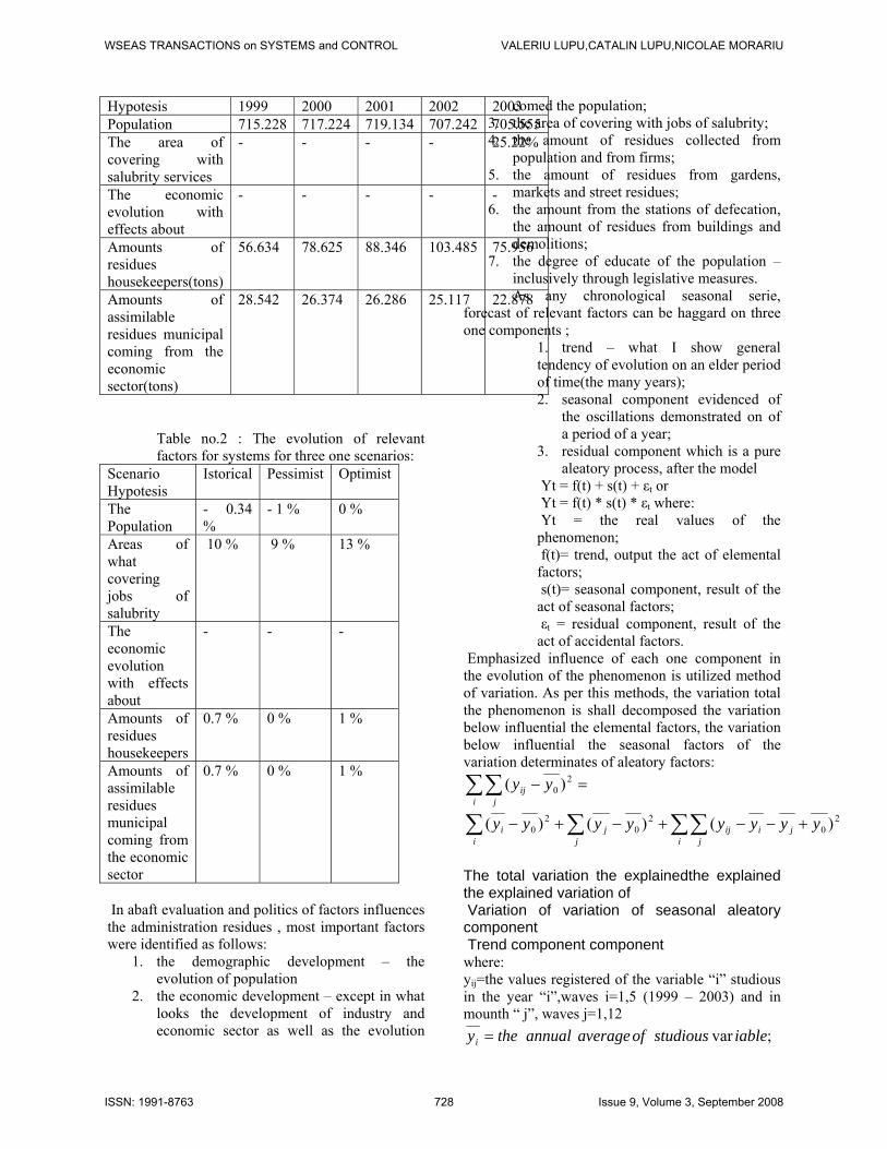
Hypotesis 1999 2000 2001 2002 2003 Population 715.228 717.224 719.134 707.242 705.555The area of covering with salubrity services

- - - - 25.22%

The economic evolution with effects about

- - - - -

Amounts of residues housekeepers(tons)

56.634 78.625 88.346 103.485 75.956

Amounts of assimilable residues municipal coming from the economic sector(tons)

28.542 26.374 26.286 25.117 22.878

Table no.2 : The evolution of relevant factors for systems for three one scenarios:

Scenario Hypotesis

Istorical Pessimist Optimist

The Population

- 0.34 %

- 1 % 0 %

Areas of what covering jobs of salubrity

10 % 9 % 13 %

The economic evolution with effects about

- - -

Amounts of residues housekeepers

0.7 % 0 % 1 %

Amounts of assimilable residues municipal coming from the economic sector

0.7 % 0 % 1 %

In abaft evaluation and politics of factors influences the administration residues , most important factors were identified as follows:

1. the demographic development – the evolution of population

2. the economic development – except in what looks the development of industry and economic sector as well as the evolution

comed the population; 3. the area of covering with jobs of salubrity; 4. the amount of residues collected from

population and from firms; 5. the amount of residues from gardens,

markets and street residues; 6. the amount from the stations of defecation,

the amount of residues from buildings and demolitions;

7. the degree of educate of the population – inclusively through legislative measures. As any chronological seasonal serie,

forecast of relevant factors can be haggard on three one components ;

1. trend – what I show general tendency of evolution on an elder period of time(the many years); 2. seasonal component evidenced of

the oscillations demonstrated on of a period of a year;

3. residual component which is a pure aleatory process, after the model

Yt = f(t) + s(t) + εt or Yt = f(t) * s(t) * εt where: Yt = the real values of the phenomenon; f(t)= trend, output the act of elemental factors; s(t)= seasonal component, result of the act of seasonal factors; εt = residual component, result of the act of accidental factors.

Emphasized influence of each one component in the evolution of the phenomenon is utilized method of variation. As per this methods, the variation total the phenomenon is shall decomposed the variation below influential the elemental factors, the variation below influential the seasonal factors of the variation determinates of aleatory factors:

∑∑ =−i j

ij yy 20 )(

∑∑∑∑ +−−+−+−i j

jiijj

ji

i yyyyyyyy 20

20

20 )()()(

The total variation the explainedthe explained the explained variation of Variation of variation of seasonal aleatory component Trend component component where: yij=the values registered of the variable “i” studious in the year “i”,waves i=1,5 (1999 – 2003) and in mounth “ j”, waves j=1,12

;var iablestudiousofaverageannualtheyi =



;var iablestudiousofaveragemonthlythey j =

.var0 iablestudiousofaveragegeneralthey = 3. Using the neural network to prevent waste material pollution 3.1. Introduction into the domain Modelling a neural network means to take into account some aspects of major importance in the functioning of the dynamic system, some parameters the selecting of which determining the success or failure of the network. At present, no solid theory at the basis for a functional or structural implementation of a neural web (network) in order to solve a certain problem as in fact, this process is reduced to a procedure of the type attempt-errors such being closer to art than to science. Here are some aspects to be considered for the implementation[1]:

Data processing o Frequency date (daily, weekly, monthly,

etc.); o Data type; o Scalar method.

Learning process o Starting ratio; o Moment term; o Tolerated learning error; o Maximum network rolling number; o Number of aleatory initialization of the

associated connection weights; o Dimension of the training, validation

and testing. Topology of the neural network

o Number of neurons belonging to the in/out strata;

o Number of hidden strata; o Number of neurons in cache hidden

stratum; o Type of activation functions; o Type of error function.

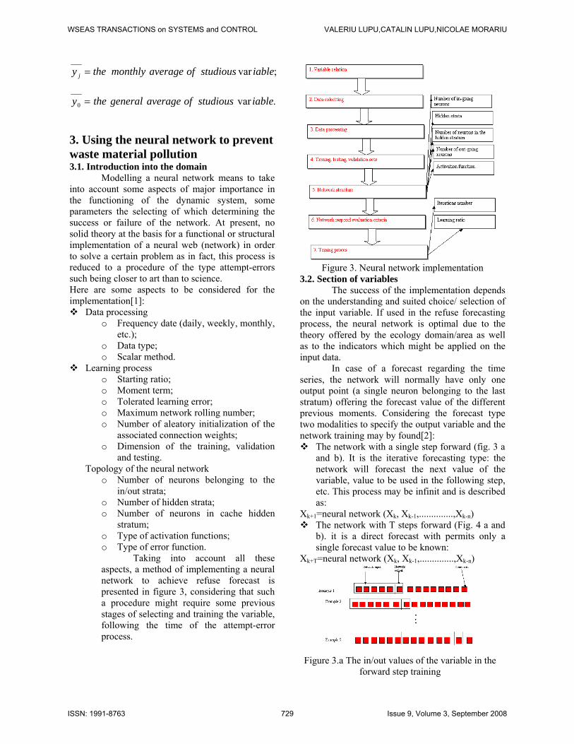
Taking into account all these aspects, a method of implementing a neural network to achieve refuse forecast is presented in figure 3, considering that such a procedure might require some previous stages of selecting and training the variable, following the time of the attempt-error process.

Figure 3. Neural network implementation

3.2. Section of variables The success of the implementation depends on the understanding and suited choice/ selection of the input variable. If used in the refuse forecasting process, the neural network is optimal due to the theory offered by the ecology domain/area as well as to the indicators which might be applied on the input data. In case of a forecast regarding the time series, the network will normally have only one output point (a single neuron belonging to the last stratum) offering the forecast value of the different previous moments. Considering the forecast type two modalities to specify the output variable and the network training may by found[2]:

The network with a single step forward (fig. 3 a and b). It is the iterative forecasting type: the network will forecast the next value of the variable, value to be used in the following step, etc. This process may be infinit and is described as:

Xk+1=neural network (Xk, Xk-1,..............,Xk-n) The network with T steps forward (Fig. 4 a and

b). it is a direct forecast with permits only a single forecast value to be known:

Xk+T=neural network (Xk, Xk-1,..............,Xk-n)

Figure 3.a The in/out values of the variable in the

forward step training



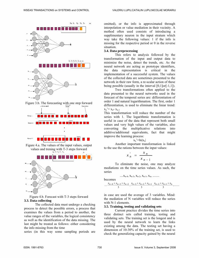
Figure 3.b. The forecasting with one step forward

Figure 4.a. The values of the input values, output

values and trening with T-3 steps forward

Figure 4.b. Forecast with T-3 steps forward

3.3. Data collecting The collected data must undergo a checking process to detect the possible errors, a process that examines the values from a period to another, the value ranges of the variables, the logical consistency as well as the identification of the data missing. The last might be treated as follows: either considering the info missing from the time series (in this way some sampling periods are

omitted), or the info is approximated through interpolation or value mediation in their vecinity. A method often used consists of introducing a supplimentary neuron in the input stratum which way take the following values: 1 if the info is missing for the respective period or 0 in the reverse situation. 3.4. Data preprocessing This refers to analysis followed by the transformation of the input and output data to minimize the noise, detect the trends, etc. As the neural network are acting as prototype identifiers, the data representation is critical in the implementation of a successful system. The values of the collected data are sometimes presented to the network in their raw form, a re-scalar action of these being possible (usually in the interval [0,1]or[-1,1]). Two transformations often applied to the data presented to the neural networks used in the forecast of the temporal series are: differentiation of order 1 and natural logarithmation. The first, order 1 differentiation, is used to eliminate the liniar trend: xn’= xn- xn-1 This transformation will reduce the number of the series with 1. The logarithmic transformation is useful in case of the data that represent both small values and very high values of the variables, also converting the multiplicative relations into additive/additional equivalents, fact that might improve the learning process:

xn’=ln|xn| Another important transformation is linked to the use the rations between the input values:

1

'

−=

n

nn x

xx

To eliminate the noise, one may analyze mediations on the time series values. As such, the series

....xn-4, xn-3, xn-2, xn-1, xn, ........ becomes

,........3

,3

,3

.... 12123234 nnnnnnnnn xxxxxxxxx ++++++ −−−−−−−−

in case are used the average of 3 variables. Mind: the mediation of N variables will reduce the series with N-1 elements. 3.5. Training, testing and validating sets Current practice divides the time series into three distinct sets called training, testing and validating sets. The training set is the longest and is used by the neural network to learn the links existing among the data. The testing set having a dimension of 10-30% of the training set, is used to check the generalizing capacity gained by the neural



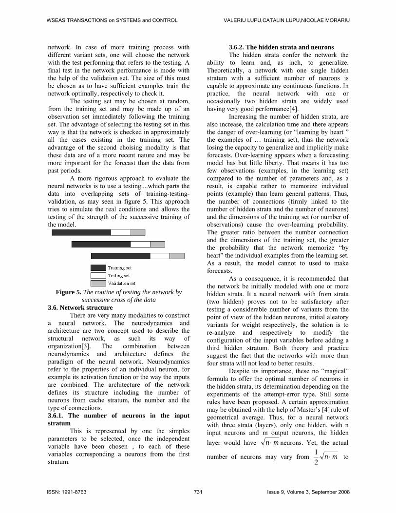
network. In case of more training process with different variant sets, one will choose the network with the test performing that refers to the testing. A final test in the network performance is mode with the help of the validation set. The size of this must be chosen as to have sufficient examples train the network optimally, respectively to check it. The testing set may be chosen at random, from the training set and may be made up of an observation set immediately following the training set. The advantage of selecting the testing set in this way is that the network is checked in approximately all the cases existing in the training set. The advantage of the second choising modality is that these data are of a more recent nature and may be more important for the forecast than the data from past periods. A more rigorous approach to evaluate the neural networks is to use a testing....which parts the data into overlapping sets of training-testing-validation, as may seen in figure 5. This approach tries to simulate the real conditions and allows the testing of the strength of the successive training of the model.

Figure 5. The routine of testing the network by

successive cross of the data 3.6. Network structure There are very many modalities to construct a neural network. The neurodynamics and architecture are two concept used to describe the structural network, as such its way of organization[3]. The combination between neurodynamics and architecture defines the paradigm of the neural network. Neurodynamics refer to the properties of an individual neuron, for example its activation function or the way the inputs are combined. The architecture of the network defines its structure including the number of neurons from cache stratum, the number and the type of connections. 3.6.1. The number of neurons in the input stratum This is represented by one the simples parameters to be selected, once the independent variable have been chosen , to each of these variables corresponding a neurons from the first stratum.

3.6.2. The hidden strata and neurons The hidden strata confer the network the ability to learn and, as inch, to generalize. Theoretically, a network with one single hidden stratum with a sufficient number of neurons is capable to approximate any continuous functions. In practice, the neural network with one or occasionally two hidden strata are widely used having very good performance[4]. Increasing the number of hidden strata, are also increase, the calculation time and there appears the danger of over-learning (or “learning by heart ” the examples of … training set), thus the network losing the capacity to generalize and implicitly make forecasts. Over-learning appears when a forecasting model has but little liberty. That means it has too few observations (examples, in the learning set) compared to the number of parameters and, as a result, is capable rather to memorize individual points (example) than learn general patterns. Thus, the number of connections (firmly linked to the number of hidden strata and the number of neurons) and the dimensions of the training set (or number of observations) cause the over-learning probability. The greater ratio between the number connection and the dimensions of the training set, the greater the probability that the network memorize “by heart” the individual examples from the learning set. As a result, the model cannot to used to make forecasts. As a consequence, it is recommended that the network be initially modeled with one or more hidden strata. It a neural network with from strata (two hidden) proves not to be satisfactory after testing a considerable number of variants from the point of view of the hidden neurons, initial aleatory variants for weight respectively, the solution is to re-analyze and respectively to modify the configuration of the input variables before adding a third hidden stratum. Both theory and practice suggest the fact that the networks with more than four strata will not lead to better results. Despite its importance, these no “magical” formula to offer the optimal number of neurons in the hidden strata, its determination depending on the experiments of the attempt-error type. Still some rules have been proposed. A certain approximation may be obtained with the help of Master’s [4] rule of geometrical average. Thus, for a neural network with three strata (layers), only one hidden, with n input neurons and m output neurons, the hidden layer would have mn ⋅ neurons. Yet, the actual

number of neurons may vary from mn ⋅21

to



2 mn ⋅ , depending on the complexity of the problem. Baily and Thompson suggested the fact that the number of neurons from the hidden stratum should be equal to 75% of the number of input neurons. Katz [6] shows that the optimum number

of neurons is generally between 21

n and 3n. Ersoy

proposes the doubling of the neuron number till the moment the performance of the network in the testing let is deteriorated. Klimasauskas [7] suggests the fact that there should be 5 times more examples in the training set than the number of connection, fact that determines a superior limited for the number of input neurons and of the hidden ones. It is important to observe the rules to calculate the number of hidden neurons as a multiple of the number of input neurons, these rules imply that the training set is at least two times greater than the number of connections and preferably 4-5 times greater. If the condition is not fulfilled, then these rules casily lead to over-learning cases as the number of the hidden neurons (and implicitly the number of connections). The solution is either to increase the training set (if possible) or to establish a superior limit regarding the input neurons so as the number of connections be at least halt of the dimension of the learning set. In this case, the selection of the input variables become critical. Selecting the optimum number of hidden neurons asks for experimentation. Three methods often used are: the fixed method, the constructive methods the distructive methods. In the first approach, a group of neural networks, cache group with a different number of hidden neurons and trained and cache is evaluated on the testing set initialized aleatory weights. The increment (increase) regarding the number of hidden neurons may be 1, 2 or more depending on the computational resources at hand. Considering the evaluation criteria (sum of the quarter errors afferent to cache testing set) as a function of the number of hidden neurons for cache network taken into consideration, one may obtain a graph the minimum of which will indicate the network most capable to generate. This approach is greatly time consuming but generally offer very good results The constructive and distructive methods change the number of hidden neurons in the learning time instead of creating some separate networks as in the previous approach. The constructive approach refers to adding up the hidden neurons till the performance of the network deteriorates. The distructive approach is similar, the hidden neurons being eliminated successively in the training period.

Irrispective of the chosen method to select the number of hidden neurons, the rule is to always select the testing set with the smallest number of neurons.

3.6.3. The number of neurons in the output lager (stratum) The neural networks with multiple outputs, especially when they are disposed, will produce result inferior to those that use a single final neuron. A network trains it self by modifying the weight of the connections so that the average error of final neurons output be minimal. For example, a network that makes forecasts both for a month and for six month (having, as such, two neurons in the output layer) will ask efforts to minimize the errors introduced most probably by the output of those 6 month in advance. As a result, there will not be many improvements of the forecast with a month in advance, the solution in this case being to train two separate networks of cache forecasting type. This specialization determins the attempt-error procedure to become simpler or every network is much simpler existing as result, fewer parameters to be adjusted to obtain the final model. 3.6.4. Activation functions The transfer or activation function represent mathematical functions that determine the output of a processing element namely, the neuron. They are also reffered to as transformations activation and limit functions. The majority of the neural network use o sigmoid function but many others have been proposed. The motif of the transfer function is to prevent the output to attain very high values that could “paralize” the network and, as a result, to act inhibitively on learning[5]. The non-liniar transfer functions are not used in case of the non-liniar mappings and classifications. The sigmoid function is often used in case of the time series due to its non-liniarity, continuity and derivation capacity, properties that are good to learn the network. Klimasauskas asserts that if the network must learn a medium behaviour, a sigmoid function should be used, while when learning proposes deviations from the average (medium), the hyperbolic tangent function be haves the test. The limit and the grade function are recommended for binary variables as the sigmoid function come close to 0 and 1 asymptotic. In a standard neural network the uses the learning algorithm with error retropropagation, the neurons of the input layer normaly use liniar transfer functions while all the neurons use the sigmoid function. The input data are usually scaled in the interval [0,1] or [-1,1] for be in agreement with the



type of the used activation function. The liniar scalation or that with the help of the average/error are two of the most used methods. In case of the liniar scalation, all the observations are liniary placed between the maximum and the minimum value as in the formula:

VS=FTmin+(FTmax–FTmin)minmax

min

DDDD−−

⋅

where VS = scalated value FTmin şi FTmax – minimum and maximum values and current of the transfer function Dmin, Dmax, D – minimum and maximum values and current of the scalated data (observation). The simple liniar scalation does not change the uniformity of the distribution, it simply re-scale the data in the field corresponding the transfer function. Thus, in some situation are adequate learning cannot be achieved because of the form in witch the input data are presented. In case of scalation using the average value and derivation, all the value, all plus or minus values taken several times, the derivations from the average mapped to 1 or 0. All the other value are liniary scaled between 0 or 1. This type of scalation created a rather uniform distribution. 3.7. Training the neural network Training a neural network to learn the patterns existing in input data means successive example with connect, knows answers. The aim is to find a set of weights afferent to the connections between the neurons to correspond to a minimum of the error function. Except the case when the model is over-learned, this set will offer a good generalization. The multilayer perceptron uses a learning algorithm based on the decrease of the gradient and the edges adjustment to be directed towards a minimum of the error surface. Finding the global minimum is not guaranteed as the error surface may present a series of local minimum values in which the network may block it self. A term of moment and 5 to 10 aleatory sets of initial weights, with which the learning algorithm starts, may improve the chances to attain the global minimum. There are two great concepts regarding the moment learning should be stopped. The first stresses the danger to fall to a local minimum and on the difficulty to obtain the global minimum. The algorithm should, as such, be stopped when there is no improvement of the error function value, considering a sufficient number of aleatory initializations of the network weights. The point where the network no longer shows improvements

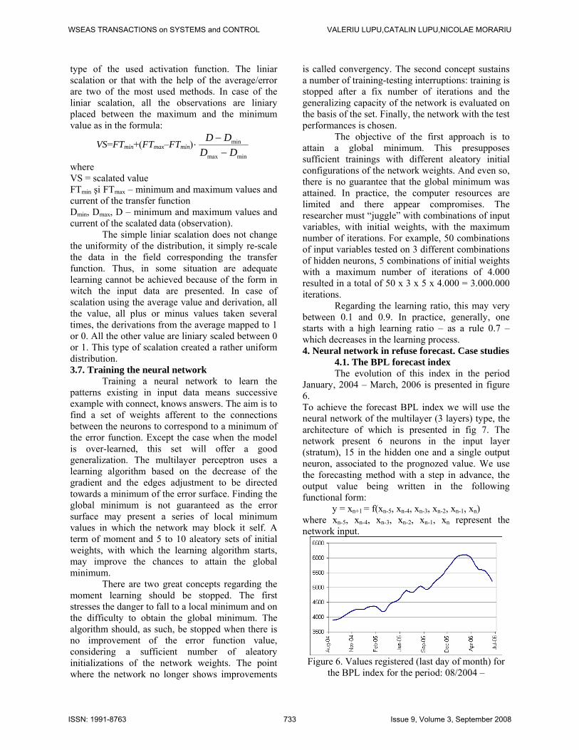
is called convergency. The second concept sustains a number of training-testing interruptions: training is stopped after a fix number of iterations and the generalizing capacity of the network is evaluated on the basis of the set. Finally, the network with the test performances is chosen. The objective of the first approach is to attain a global minimum. This presupposes sufficient trainings with different aleatory initial configurations of the network weights. And even so, there is no guarantee that the global minimum was attained. In practice, the computer resources are limited and there appear compromises. The researcher must “juggle” with combinations of input variables, with initial weights, with the maximum number of iterations. For example, 50 combinations of input variables tested on 3 different combinations of hidden neurons, 5 combinations of initial weights with a maximum number of iterations of 4.000 resulted in a total of 50 x 3 x 5 x 4.000 = 3.000.000 iterations. Regarding the learning ratio, this may very between 0.1 and 0.9. In practice, generally, one starts with a high learning ratio – as a rule 0.7 – which decreases in the learning process. 4. Neural network in refuse forecast. Case studies 4.1. The BPL forecast index The evolution of this index in the period January, 2004 – March, 2006 is presented in figure 6. To achieve the forecast BPL index we will use the neural network of the multilayer (3 layers) type, the architecture of which is presented in fig 7. The network present 6 neurons in the input layer (stratum), 15 in the hidden one and a single output neuron, associated to the prognozed value. We use the forecasting method with a step in advance, the output value being written in the following functional form:

y = xn+1 = f(xn-5, xn-4, xn-3, xn-2, xn-1, xn) where xn-5, xn-4, xn-3, xn-2, xn-1, xn represent the network input.

Figure 6. Values registered (last day of month) for

the BPL index for the period: 08/2004 –



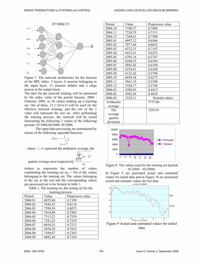
07/2006[17]

Figure 7. The network architecture for the forecast of the BPL index. 3 layers, 6 neurons belonging to the input layer, 15 neurons hidden and a singe neuron in the output layer. The date for the network training will be presented by the index value of the period January, 2004 - February 2006, so 26 values making up a learning set. Out of these, 15 (=26-6-5) will be used for the effective network training, and the rest of the 5 value will represent the test set. After performing the training process, the network will be tested forecasting the following 3 values of the following periods: 03/2006,04/2006, 05/2006. The input data processing are norminated by means of the following signoidal function:

σxx

e

xf−

+

=

1

1)(

where: x , σ represent the arithmetic average, the

quarter average error respectively k

n

ii

n

xxk

∑=

−1

2)(

(where nk represents the number of values constituting the learning set (nk = 34) of the values belonging to the training set. The values belonging to the set, to the test and the corresponding values pre-processed are to be formed in table 1.

Table 1. The training set, the testing set for the learning process

Period Value Preprocess value 2004.01 6835,60 0,7199 2004.02 7644,55 0,8118 2004.03 7599,39 0,8073 2004.04 7414,68 0,7883 2004.05 7313,21 0,7539 2004.06 7241,23 0,7259 2004.07 6854,25 0,7213 2004.08 3654,29 0,7633 2004.08 7109,67 0,7363 2004.09 6882,44 0,7336

Period Value Preprocess value 2004.10 7190,37 0,7696 2004.11 7224,79 0,7151 2004.12 7344,61 0,7500 2005.01 6897,12 0,6566 2005.02 7077,44 0,6653 2005.03 6372,33 0,7147 2005.04 6433,61 0,6235 2005.05 6795,14 0,5747 2005.06 6208,35 0,6394 2005.07 5892,42 0,6198 2005.08 6254,41 0,6100 2005.09 6123,26 0,5796 2005.10 6058,38 0,4272 2005.11 5861,19 0,3380 2005.12 5188,17 0,3748 2006.01 4308,83 0,4413 2006.02 4382,56 0,4628 2006.03 3320,11 Periods/values Arithmetic

average 5737,06

The average quarter

deviation

1293,91

0

2000

4000

6000

8000

10000

1 5 9 13 17 21 25

PerioadaValoare

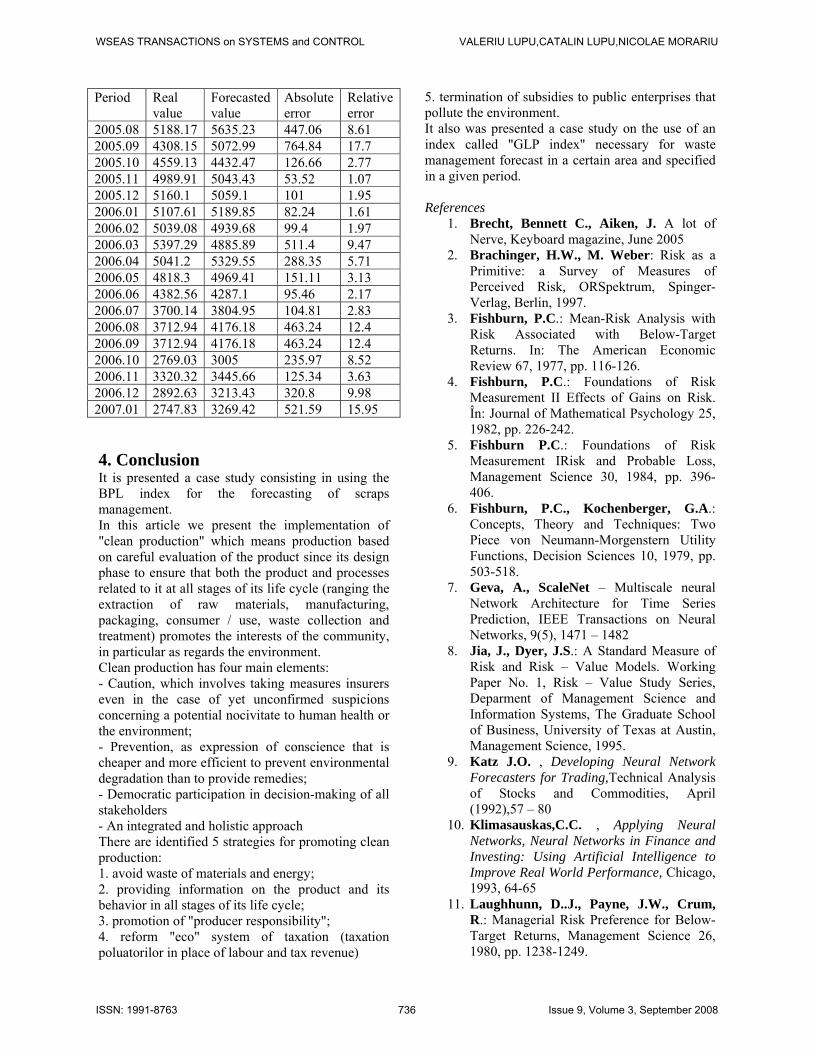
Figure 8. The values used for the training set (period

01/2004 – 02/2006) In Figure 9 are presented actual and estimated values for initial data and in Figure 10 are presented actual and estimate values for test data.

Figure 9 Actual and estimated values for initial

data



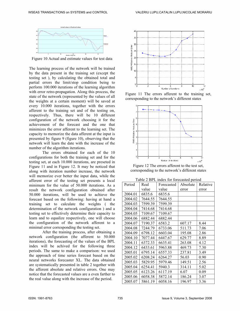
Figure 10 Actual and estimate values for test data

The learning process of the network will be trained by the data present in the training set (except the testing set ), by calculating the obtained total and partial errors the limit/stop condition being to perform 100.000 iterations of the learning algorithm with error retro-propagation. Along this process, the state of the network (represented by the values of all the weights at a certain moment) will be saved at every 10.000 iterations, together with the errors afferent to the training set and of the testing on, respectively. Thus, there will be 10 different configuration of the network choosing it for the achievement of the forecast and the one that minimizes the error afferent to the learning set. The capacity to memorize the data afferent at the input is presented by figure 9 (figure 10), observing that the network will learn the date with the increase of the number of the algorithm iterations. The errors obtained for each of the 10 configurations for both the training set and for the testing set, at each 10.000 iterations, are preseted in Figure 11 and in Figure 12. It may be noticed that along with iteration number increase, the network will memorize ever better the input data, while the afferent error of the testing set presents a local minimum for the value of 50.000 iterations. As a result the network configuration obtained after 50.000 iterations, will be used to achieve the forecast based on the following: having at hand a training set to calculate the weights ( the determination of the network configuration ) and a testing set to effectively determine their capacity to learn and to equalize respectively, one will choose the configuration of the network afferent to a minimal error corresponding the testing set. After the training process, after obtaining a network configuration (the afferent to 50.000 iterations), the forecasting of the values of the BPL index will be achived for the following three periods. The same to make a comparison: we used the approach of time series forecast based on the neural networks forecaster XL. The data obtained are systematically presented in table 2 together with the afferent absolute and relative errors. One may notice that the forecasted values are a even farther to the real value along with the increase of the period.

Figure 11 The errors afferent to the training set, corresponding to the network’s different states

Figure 12 The errors afferent to the test set,

corresponding to the network’s different states

Table 2 BPL index for forecasted period Period Real

value Forecasted value

Absolute error

Relative error

2004.01 6835.6 6835.6 2004.02 7644.55 7644.55 2004.03 7599.39 7599.39 2004.04 7414.68 7414.68 2004.05 7109.67 7109.67 2004.06 6882.44 6882.44 2004.07 7190.37 6583.2 607.17 8.44 2004.08 7244.79 6733.06 511.73 7.06 2004.09 6798.12 6603.04 195.08 2.86 2004.10 7077.44 6447.67 629.77 8.89 2004.11 6372.33 6635.41 263.08 4.12 2004.12 6433.61 5963.88 469.73 7.30 2005.01 6795.14 6557.33 237.81 3.49 2005.02 6208.24 6264.27 56.03 0.90 2005.03 5829.95 5979.46 149.51 2.56 2005.04 6254.41 5940.3 314.11 5.02 2005.05 6123.26 6117.19 6.07 0.09 2005.06 6058.38 5872.14 186.24 3.07 2005.07 5861.19 6058.16 196.97 3.36



Period Real value

Forecasted value

Absolute error

Relative error

2005.08 5188.17 5635.23 447.06 8.61 2005.09 4308.15 5072.99 764.84 17.7 2005.10 4559.13 4432.47 126.66 2.77 2005.11 4989.91 5043.43 53.52 1.07 2005.12 5160.1 5059.1 101 1.95 2006.01 5107.61 5189.85 82.24 1.61 2006.02 5039.08 4939.68 99.4 1.97 2006.03 5397.29 4885.89 511.4 9.47 2006.04 5041.2 5329.55 288.35 5.71 2006.05 4818.3 4969.41 151.11 3.13 2006.06 4382.56 4287.1 95.46 2.17 2006.07 3700.14 3804.95 104.81 2.83 2006.08 3712.94 4176.18 463.24 12.4 2006.09 3712.94 4176.18 463.24 12.4 2006.10 2769.03 3005 235.97 8.52 2006.11 3320.32 3445.66 125.34 3.63 2006.12 2892.63 3213.43 320.8 9.98 2007.01 2747.83 3269.42 521.59 15.95 4. Conclusion It is presented a case study consisting in using the BPL index for the forecasting of scraps management. In this article we present the implementation of "clean production" which means production based on careful evaluation of the product since its design phase to ensure that both the product and processes related to it at all stages of its life cycle (ranging the extraction of raw materials, manufacturing, packaging, consumer / use, waste collection and treatment) promotes the interests of the community, in particular as regards the environment. Clean production has four main elements: - Caution, which involves taking measures insurers even in the case of yet unconfirmed suspicions concerning a potential nocivitate to human health or the environment; - Prevention, as expression of conscience that is cheaper and more efficient to prevent environmental degradation than to provide remedies; - Democratic participation in decision-making of all stakeholders - An integrated and holistic approach There are identified 5 strategies for promoting clean production: 1. avoid waste of materials and energy; 2. providing information on the product and its behavior in all stages of its life cycle; 3. promotion of "producer responsibility"; 4. reform "eco" system of taxation (taxation poluatorilor in place of labour and tax revenue)

5. termination of subsidies to public enterprises that pollute the environment. It also was presented a case study on the use of an index called "GLP index" necessary for waste management forecast in a certain area and specified in a given period. References

1. Brecht, Bennett C., Aiken, J. A lot of Nerve, Keyboard magazine, June 2005

2. Brachinger, H.W., M. Weber: Risk as a Primitive: a Survey of Measures of Perceived Risk, ORSpektrum, Spinger-Verlag, Berlin, 1997.

3. Fishburn, P.C.: Mean-Risk Analysis with Risk Associated with Below-Target Returns. In: The American Economic Review 67, 1977, pp. 116-126.

4. Fishburn, P.C.: Foundations of Risk Measurement II Effects of Gains on Risk. În: Journal of Mathematical Psychology 25, 1982, pp. 226-242.

5. Fishburn P.C.: Foundations of Risk Measurement IRisk and Probable Loss, Management Science 30, 1984, pp. 396-406.

6. Fishburn, P.C., Kochenberger, G.A.: Concepts, Theory and Techniques: Two Piece von Neumann-Morgenstern Utility Functions, Decision Sciences 10, 1979, pp. 503-518.

7. Geva, A., ScaleNet – Multiscale neural Network Architecture for Time Series Prediction, IEEE Transactions on Neural Networks, 9(5), 1471 – 1482

8. Jia, J., Dyer, J.S.: A Standard Measure of Risk and Risk – Value Models. Working Paper No. 1, Risk – Value Study Series, Deparment of Management Science and Information Systems, The Graduate School of Business, University of Texas at Austin, Management Science, 1995.

9. Katz J.O. , Developing Neural Network Forecasters for Trading,Technical Analysis of Stocks and Commodities, April (1992),57 – 80

10. Klimasauskas,C.C. , Applying Neural Networks, Neural Networks in Finance and Investing: Using Artificial Intelligence to Improve Real World Performance, Chicago, 1993, 64-65

11. Laughhunn, D..J., Payne, J.W., Crum, R.: Managerial Risk Preference for Below-Target Returns, Management Science 26, 1980, pp. 1238-1249.



Documents

The implementation of clean production and the use of ... · PDF fileThe implementation of clean production and the use of neural networks in forecasting waste management ... 2. the