Embed Size (px)
Citation preview
The Impact of Pessimistic Expectations on the Effects of COVID-19-Induced Uncertainty in the Euro Area
Giovanni Pellegrino [email protected]
UNIVERSITY OF AARHUS
Gabriel Züllig [email protected]
DANMARKS NATIONALBANK AND UNIVERSITY OF COPENHAGEN
Federico Ravenna [email protected]
DANMARKS NATIONALBANK
The Working Papers of Danmarks Nationalbank describe research
and development, often still ongoing, as a contribution to the
professional debate.
The viewpoints and conclusions stated are the responsibility of the individual contributors, and do not necessarily reflect the views of Danmarks Nationalbank.
2 6 O C T O B E R 2 0 2 0 — N O . 1 6 2
WORK ING PAPE R — DANMARK S NAT IONA LBANK
2 6 O C T O B E R 2 0 2 0 — N O . 1 6 2
Abstract We estimate a monthly Interacted-VAR model for
euro area macroeconomic aggregates allowing for
the impact of uncertainty shocks to depend on the
average outlook of the economy measured by
survey data. We find that, in response to an
uncertainty shock, the peak decrease in industrial
production and inflation is around three and a half
times larger during pessimistic times. We build
scenarios for a path of innovations consistent with
the increase in the observed VSTOXX measure of
uncertainty at the outset of the COVID-19 epidemics
in February and March 2020. Industrial production
is predicted to experience a year-over-year peak
loss of between 15.1% and 19% in the fourth
quarter of 2020, and subsequently to recover with a
rebound to pre-crisis levels between May and
August 2021. The large impact is the result of an
extreme shock to uncertainty occurring at a time of
very negative expectations for the economic
outlook.
Resume Vi estimerer en månedlig interaktiv VAR-model for
makroøkonomiske variable i euroområdet.
Modellen tillader, at effekten af usikkerhedsstød
afhænger af de gennemsnitlige økonomiske
udsigter målt ved spørgeskemaundersøgelser. Vi
finder, at maksimalfaldet i industriproduktionen og
inflationen efter et stød til usikkerheden er 3,5
gange større, når de økonomiske udsigter er
pessimistiske. Vi konstruerer scenarier for en
stødrække, som er i overensstemmelse med
stigningen observeret i VSTOXX-usikkerhedsmålet i
begyndelsen af COVID-19-pandemien i februar og
marts 2020. Modellen forudsiger, at det maksimale
fald i industriproduktionen er på mellem 15,1 og 19
% målt år-til-år og indtræffer i fjerde kvartal af 2020.
Herefter forudsiger modellen, at
industriproduktionen begynder at genoprettes til
niveauet før krisen mellem maj og august 2021. Den
store effekt skyldes et ekstremt stød til
usikkerheden, som rammer økonomien på et
tidspunkt, hvor de økonomiske udsigter er meget
negative.
The Impact of Pessimistic Expectations on the Effects of COVID-19-Induced Uncertainty in the Euro Area
Acknowledgements The authors wish to thank Henrik Yde Andersen,
Efrem Castelnuovo, Menzie Chinn, Alessia
Paccagnini, Michele Piffer, and Carl Walsh for
providing comments, and Roberta Friz for
providing the granular data on the basis of the
European Commission’s consumer and business
surveys. The authors alone are responsible for any
remaining errors.
Key words Current economic and monetary trends, Economic
activity and employment, Models
JEL classification C32; E32
The Impact of Pessimistic Expectations on the Effects of
COVID-19-Induced Uncertainty in the Euro Area∗
Giovanni Pellegrino Federico Ravenna Gabriel Züllig
Aarhus University
Danmarks NationalbankUniversity of CopenhagenHEC Montreal, CEPR
Danmarks NationalbankUniversity of Copenhagen
July 2020
Abstract
We estimate a monthly Interacted-VAR model for euro area macroeconomic aggregates al-
lowing for the impact of uncertainty shocks to depend on the average outlook of the economy
measured by survey data. We find that, in response to an uncertainty shock, the peak decrease
in industrial production and inflation is around three and a half times larger during pessimistic
times. We build scenarios for a path of innovations consistent with the increase in the observed
VSTOXX measure of uncertainty at the outset of the COVID-19 epidemics in February and
March 2020. Industrial production is predicted to experience a year-over-year peak loss of be-
tween 15.1% and 19% in the fourth quarter of 2020, and subsequently to recover with a rebound
to pre-crisis levels between May and August 2021. The large impact is the result of an extreme
shock to uncertainty occurring at a time of very negative expectations for the economic outlook.
Keywords: COVID-19, Uncertainty Shocks, Non-Linear Structural Vector AutoRegressions,
Consumer Confidence. JEL codes: C32, E32.
∗ We thank Henrik Yde Andersen, Efrem Castelnuovo, Menzie Chinn, Alessia Paccagnini, Michele Piffer, CarlWalsh for providing comments, and Roberta Friz for providing the granular data at the basis of the EuropeanCommission consumer and business surveys. Contacts: Giovanni Pellegrino: [email protected] ; GabrielZüllig: [email protected] ; Federico Ravenna: [email protected]. The viewpoints and conclu-sions stated are the responsibility of the individual contributors, and do not necessarily reflect the views of DanmarksNationalbank. The authors alone are responsible for any remaining errors.
1 Introduction
The social distancing measures imposed worldwide in response to the COVID-19 epidemic have
resulted in the partial shutdown of economic activity, and immediate losses in output.1 As countries
started planning a gradual reopening of the economy in April 2020, expectations for the future
were at their lowest, reflecting a pessimistic outlook for the future.2 At the same time, measures of
uncertainty were still very high, after having experienced levels comparable to those of the global
financial crisis.3
Using a nonlinear Interacted VAR specification, we assess the effects of heightened uncertainty
in the presence of pessimistic expectations for the future economic outlook in the euro area, and
estimate the macroeconomic impact of the COVID-19-induced uncertainty spike.
The observed increase in uncertainty measures during the COVID-19 pandemic can be inter-
preted as a perceived increase in the probability of very negative outcomes - for example, future
pandemic waves leading to protracted economic lockdowns — as well as very positive outcomes,
such as the rapid procurement of a vaccine or effective antiviral drugs, and a fast rebound of eco-
nomic activity. It is well known that unexpected surges or "shocks" in uncertainty have a negative
effect on real activity (see, e.g., Bloom (2009), Mumtaz and Zanetti (2013), Bachmann, Elstner,
and Sims (2013), Jurado, Ludvigson, and Ng (2015), Fernández-Villaverde, Guerrón-Quintana,
Kuester, and Rubio-Ramírez (2015), Leduc and Liu (2016), Baker, Bloom, and Davis (2016), Basu
and Bundick (2017), Piffer and Podstawski (2018), Ludvigson, Ma, and Ng (2019)). This outcome
can be explained by risk-averse consumers increasing precautionary savings against a rise in the
risk of possible negative future outcomes, or by firms postponing partially-irreversible investment
to the future and adopting a "wait and see" behavior (see, e.g., Caballero (1990) and Bernanke
(1983), respectively).
Given the recent COVID-19-induced uncertainty shock, similar incentives to modify households’
and firms’optimal choices would be at work during this pandemic, with negative effects on output
that will add to those given by the lockdowns, and may potentially last longer than the lockdowns.
1By the second half of April 2020, the euro zone-wide composite Purchasing Manager Index (PMI) hit an all-timelow of 13.5, implying the eurozone economy had suffered the steepest ever fall in manufacturing and services activity(European Commission, 2020).
2The German ZEW sentiment index, and the consumer confidence indicator released by the European Commissionin April 2020 signaled a confidence level approaching the number reached during the 2008-2009 financial crisis.
3Baker, Bloom, Davis, and Terry (2020) document the recent enormous increase in economic uncertainty asmeasured by several US indicators: the VIX index; the U.S. Economic Policy Uncertainty Index; several survey-based measures reporting uncertainty about the outlook among firms.
2
This is confirmed by recent Structural Vector AutoRegression (VAR) studies on the impact of
COVID-19 uncertainty by Baker, Bloom, Davis, and Terry (2020) —estimating a peak impact on
year-over-year United States GDP growth of about 5.5% —and Leduc and Liu (2020), estimating
an impact on United States unemployment peaking at one percentage points after 12 months.
As regards the global effects of the COVID-19 uncertainty shock, Caggiano, Castelnuovo, and
Kima (2020) predict the cumulative loss in world output one year after the shock to be about
14%. However, these studies employ linear VAR models and hence cannot account for the unusual
circumstances the economy is facing in terms of both uncertainty and pessimistic outlook during the
current COVID-19 pandemic. Further, none of the aforementioned papers study the consequences
of the COVID-19 uncertainty shock for the euro area economy, the economy most hit at the time
of writing.4
We provide two novel sets of results by estimating a nonlinear Interacted VAR model. First,
we empirically study the role of pessimistic expectations for future outcomes for the historical
propagation of uncertainty shocks in the euro area. Second, we make use of this novel finding to
predict the expected propagation of the COVID-19-induced uncertainty shock.
We measure expectations for the economic outlook with consumer confidence and interpret
plummeting consumer confidence as capturing pessimism about the future.5 In principle, pessimism
- i.e., a negative outlook about the future of the economy - may influence the impact of uncertainty
shocks. Given an average outlook, higher uncertainty increases the risks in the outlook: it implies
a higher chance of more extreme outcomes, or an increased probability of large upside or downside
risks. The impact of heightened risk on optimal choices may change depending on the state of the
economy, since in some states a change in the distribution of future shocks may have a larger impact
on the distribution of economic outcomes, or agents may engage in robust-control optimal behaviour
overweighing worst-case scenarios. Several economists, including contributions by Fajgelbaum,
Schaal, and Taschereau-Dumouchel (2014) and Cacciatore and Ravenna (2020) have suggested
models able to explain the time-varying impact of uncertainty shocks.
We empirically test whether pessimism amplifies the impact of uncertainty shocks by modeling
4As of 7 July 2020, Europe reported 194,515 deaths —with the most hit countries being, in order, United King-dom (44,236), Italy (34,869), France (29,920), and Spain (28,388) — and the United States 130,306 deaths (seethe global COVID-19 situation update of the European Centre for Disease Prevention and Control, available athttps://www.ecdc.europa.eu/en/geographical-distribution-2019-ncov-cases).
5Autonomous shifts in confidence have been documented to have powerful predictive implications for income andconsumption. These shifts may operate through two possible channels: they may reflect changes in ‘animal spirits’,having a direct effect on the economy, or they may reflect fundamental information, or ‘news’, about the future stateof the economy, available to consumers and not summarized by other measurable variables (Barsky and Sims (2012)).
3
a vector of euro area macroeconomic data with an Interacted VAR (IVAR) model for the period
1999m1-2020m1. The IVAR is a parsimonious nonlinear VAR model which augments a standard
linear VAR model with an interaction term to determine how the effects of a shock on one variable
depend on the level of another variable. We interact an uncertainty measure with a measure
of consumer confidence to estimate the impact of an uncertainty shock at times when consumer
confidence is in the bottom quintile of its historical distribution. Armed with this model, we
build scenarios for a path of innovations in uncertainty consistent with the COVID-19-induced
shock. In building the hypothetical response of the economy to the uncertainty shocks, we compute
Generalized IRFs (GIRFs) à la Koop, Pesaran, and Potter (1996) to account for the endogenous
evolution of the state of the economy —including its impact on uncertainty itself.6
Following the seminal work by Bloom (2009) we focus on financial uncertainty, which we measure
by the VSTOXX index, a high-frequency measure of the implied volatility of the euro STOXX 50
stock market index (the european-analogue of the VIX index for the United States). This is
important since - as shown in Ludvigson, Ma, and Ng (2019) and Angelini, Bacchiocchi, Caggiano,
and Fanelli (2019) - indicators proxying this type of uncertainty are likely to capture movements
in uncertainty which are relevant to explain the evolution of output at business cycle frequencies.
Our main results can be summarized as follows. First, we find that historically, uncertainty
shocks in the euro area have had a significant impact on the economy only during pessimistic times.
Industrial production and inflation decrease in both states of the economy, but their decrease
is much larger and more persistent during pessimistic times. The peak response of industrial
production (inflation) to a typical uncertainty shock is −1.28% (−0.11%) in pessimistic times
and −0.36% (−0.04%) in normal times. Consistently with these findings, uncertainty shocks are
found to be about three times more important in explaining business cycle fluctuations in industrial
production and inflation during pessimistic times than during normal times, respectively explaining
the 42% and 27% of the fluctuations in the two series. We also assess several alternative economic
and econometric hypotheses about the state-dependent impact of uncertainty shocks, including
global uncertainty spillovers, the role of financial factors and households mood swings, the impact
of firms’ pessimism about the outlook, the information contained in survey measures of cross-
sectional dispersion, and a Proxy SVAR specification.
Second, our estimates imply that the COVID-19 shock via its uncertainty channel alone will
6See Caggiano, Castelnuovo, and Pellegrino (2017), Pellegrino (2017) and Pellegrino (2018) for details on theestimation methodology for the IVAR model.
4
induce a long and deep recession in the euro area. In our first scenario, we hit the pessimistic-times
state of our estimated IVAR with a ten-standard deviations uncertainty shock —corresponding to
the unexpected rise in the level of the VSTOXX measure of uncertainty from February 2020 to
March 2020. Industrial production is predicted to experience a year-over-year peak loss of 15.14%
peaking after 7 months from the shock, in September 2020, and subsequently to recover with a
rebound to pre-crisis levels in May 2021. In terms of GDP, a back-of-the-envelope calculation
suggests a corresponding fall in year-over-year GDP of roughly 4.3% at peak.
We also consider two alternative scenarios where either uncertainty goes back to normal levels
much more slowly in the current situation than in the past —given that the persisting uncertainty in
delivering a vaccine could span several months —, or where a second unexpected spike in uncertainty
occurs following a possible new wave of the pandemic in the coming fall. Both scenarios would
delay the recovery and would prolong the recessionary impact by several months, yielding a larger
total loss in industrial production. In the case of a new fall-2020 wave, our simulations predict the
trough to happen in December 2020 and the rebound to start in July 2021.
Our findings lend support to the unprecedented policy responses to the pandemic, many of which
can be interpreted as providing catastrophic insurance against worst-case outcomes. Provided that
the sole impact of the COVID-19 shock via its uncertainty channel will imply large losses as well
as a slow and painful return to normality, policymakers are required to enact clear policies aimed
not only at boosting confidence in the outlook, but aimed specifically at resolving the uncertainty.
Our study is connected with the empirical literature investigating whether uncertainty shocks
have state-dependent effects according to the economic phase when a shock hits. Caggiano, Castel-
nuovo, and Groshenny (2014), Chatterjee (2018), and Caggiano, Castelnuovo, and Figueres (2020),
among others, employ non-linear Structural VAR techniques to enquire whether contractionary
vs. expansionary phases are important in determining the impact of uncertainty shocks, whereas
Alessandri and Mumtaz (2019), Angelini, Bacchiocchi, Caggiano, and Fanelli (2019), and Lhuissier
and Tripier (2019) investigate whether financial or volatility regimes are important for the real
effects of uncertainty shocks. This study focuses on the role of consumer confidence. Its forward-
lookingness allows us to pin down the role of agents expectations for the transmission of uncertainty
shocks.
The paper is structured as follows. Section 2 presents the empirical model and the data, while
section 3 documents our empirical findings. Section 4 concludes the paper.
5
2 Econometric setting
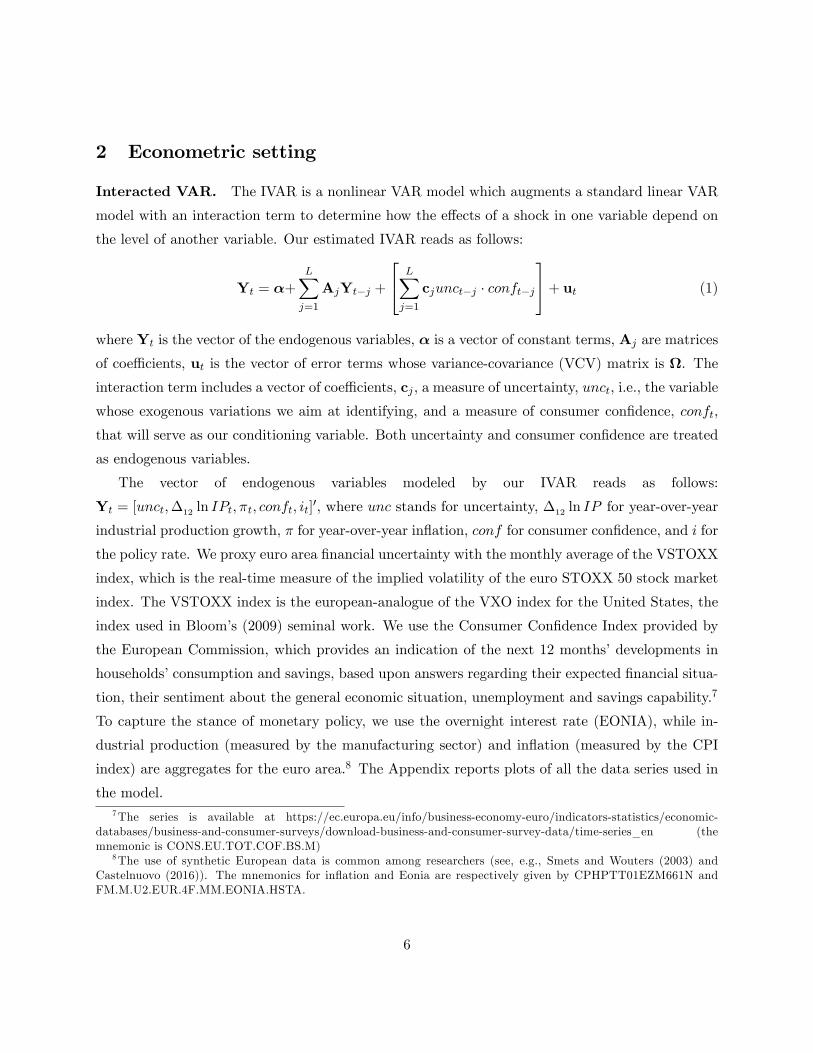
Interacted VAR. The IVAR is a nonlinear VAR model which augments a standard linear VAR
model with an interaction term to determine how the effects of a shock in one variable depend on
the level of another variable. Our estimated IVAR reads as follows:
Yt = α+
L∑j=1
AjYt−j +
L∑j=1
cjunct−j · conft−j
+ ut (1)
where Yt is the vector of the endogenous variables, α is a vector of constant terms, Aj are matrices
of coeffi cients, ut is the vector of error terms whose variance-covariance (VCV) matrix is Ω. The
interaction term includes a vector of coeffi cients, cj , a measure of uncertainty, unct, i.e., the variable
whose exogenous variations we aim at identifying, and a measure of consumer confidence, conft,
that will serve as our conditioning variable. Both uncertainty and consumer confidence are treated
as endogenous variables.
The vector of endogenous variables modeled by our IVAR reads as follows:
Yt = [unct,∆12 ln IPt, πt, conft, it]′, where unc stands for uncertainty, ∆12 ln IP for year-over-year
industrial production growth, π for year-over-year inflation, conf for consumer confidence, and i for
the policy rate. We proxy euro area financial uncertainty with the monthly average of the VSTOXX
index, which is the real-time measure of the implied volatility of the euro STOXX 50 stock market
index. The VSTOXX index is the european-analogue of the VXO index for the United States, the
index used in Bloom’s (2009) seminal work. We use the Consumer Confidence Index provided by
the European Commission, which provides an indication of the next 12 months’developments in
households’consumption and savings, based upon answers regarding their expected financial situa-
tion, their sentiment about the general economic situation, unemployment and savings capability.7
To capture the stance of monetary policy, we use the overnight interest rate (EONIA), while in-
dustrial production (measured by the manufacturing sector) and inflation (measured by the CPI
index) are aggregates for the euro area.8 The Appendix reports plots of all the data series used in
the model.7The series is available at https://ec.europa.eu/info/business-economy-euro/indicators-statistics/economic-
databases/business-and-consumer-surveys/download-business-and-consumer-survey-data/time-series_en (themnemonic is CONS.EU.TOT.COF.BS.M)
8The use of synthetic European data is common among researchers (see, e.g., Smets and Wouters (2003) andCastelnuovo (2016)). The mnemonics for inflation and Eonia are respectively given by CPHPTT01EZM661N andFM.M.U2.EUR.4F.MM.EONIA.HSTA.
6
Relative to alternative nonlinear VARs like Smooth-Transition VARs and Threshold VARs,
the IVAR is particularly appealing in addressing our research question. It enables us to model
the interaction between uncertainty and consumer confidence in a parsimonious manner — as it
does not require parametric choices for any threshold or transition function in the estimation
procedure —, and, at the same time, the IVAR can estimate the economy’s response conditional
on very low consumer confidence since the definition of a pessimistic regime is only used when
simulating generalized impulse response functions conditional on a given initial state, hence making
the responses less sensitive to outliers in a particular regime.
The IVAR methodology has been shown through Monte Carlo simulations to be able to recover
the true state-dependent impulse responses to an uncertainty shock as implied by a state-of-the-art
nonlinear DSGE framework solved via a third-order approximation around its stochastic steady
state (Andreasen, Caggiano, Castelnuovo, and Pellegrino (2020)). See Caggiano, Castelnuovo, and
Pellegrino (2017), Pellegrino (2017) and Pellegrino (2018) for details on the estimation methodology
for the IVAR model. The Appendix provides additional information on the estimation and the
GIRF algorithm.
We estimate the IVARmodel based on the 1999m1-2020m1 sample. The starting date is dictated
by the availability of the VSTOXX index and coincides with the establishment of the euro area.
The model is estimated by OLS. We use four lags as suggested by the AIC statistic. A multivariate
LR test rejects the null of linearity against our IVAR model (p− value = 0.00).
GIRFs for normal and pessimistic times. We compute GIRFs à la Koop, Pesaran, and
Potter (1996) to account for the endogenous response of consumer confidence to an uncertainty
shock and the feedbacks this can have on the dynamics of the economy. GIRFs acknowledge the
fact that, in a fully nonlinear model, responses depend on the sign of the shock, the size of the
shock, and initial conditions. Theoretically, the GIRF at horizon h of the vector Y to a shock in
date t, δt, computed conditional on an initial condition, $t−1 = Yt−1, ...,Yt−L, is given by thefollowing difference of conditional expectations:
GIRFY,t(h, δt,$t−1) = E [Yt+h | δt,$t−1]− E [Yt+h |$t−1] , h = 0, 1, . . . ,H. (2)
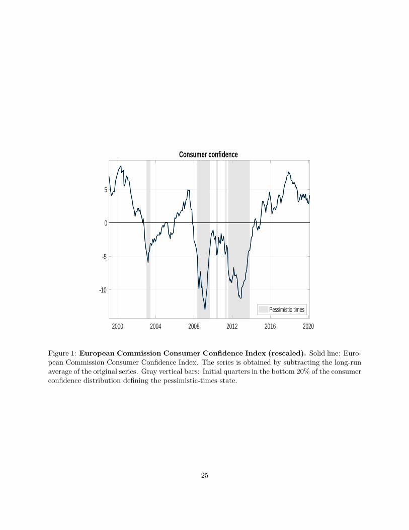
We are interested in computing the GIRFs to an uncertainty shock for normal and pessimistic
times. We define the "pessimistic times" state to be characterized by the initial months correspond-
ing to the bottom 20% of the consumer confidence distribution, while the "normal times" state is
7
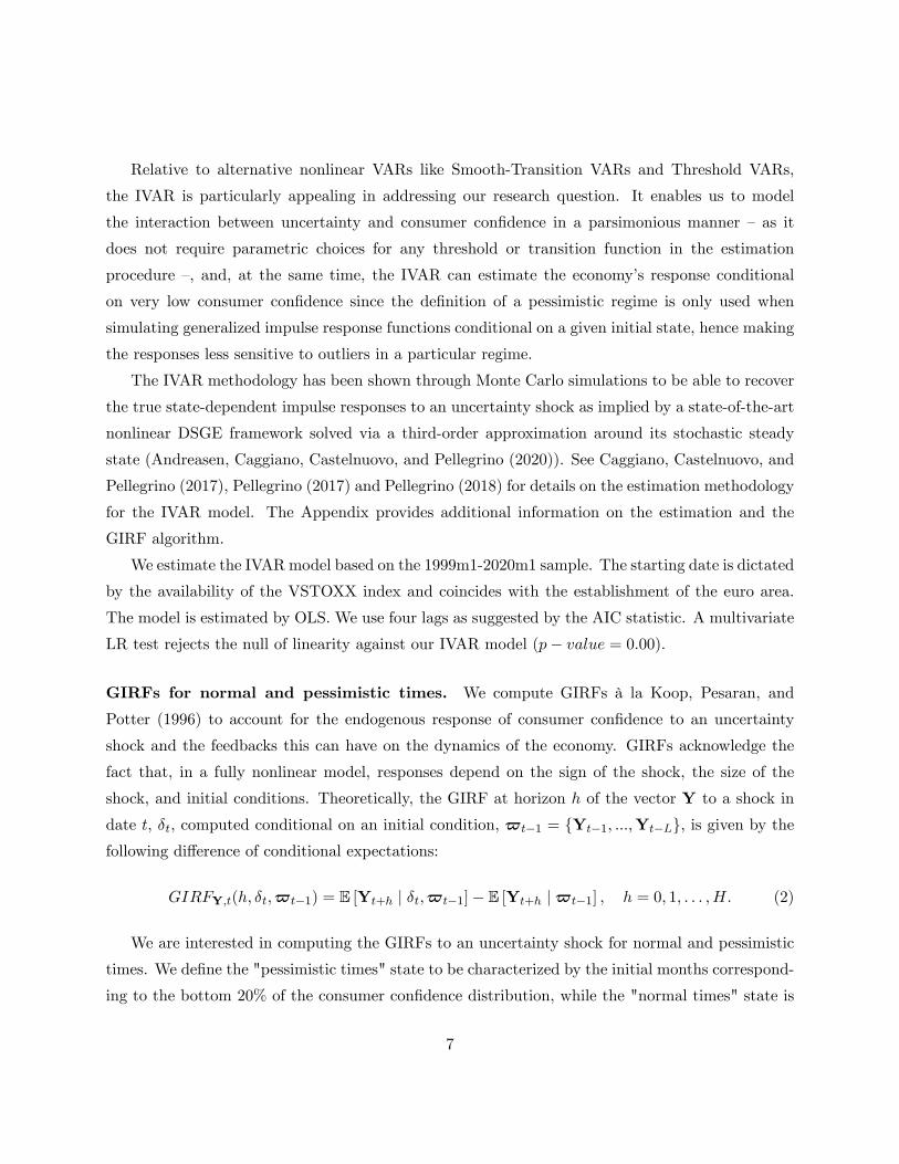
defined by all other initial months in the sample. Figure 1 plots consumer confidence for the euro
area and provides a visual representation of the two states. Pessimistic times mostly capture the
period of the great financial crisis of 2008-2009 and the sovereign debt crisis of 2011-2013 but also
capture the setback in confidence in 2003.
Uncertainty shocks are identified by means of a Cholesky decomposition with recursive structure
given by the ordering of the variables in the vector Y above, i.e., [unc,∆12 ln IP, π, conf, i]′. Order-
ing the uncertainty proxy before macroeconomic aggregates in the vector allows real and nominal
variables to react on impact, and it is a common choice in the literature (see, among others, Bloom
(2009), Caggiano, Castelnuovo, and Groshenny (2014), Fernández-Villaverde, Guerrón-Quintana,
Kuester, and Rubio-Ramírez (2015), Leduc and Liu (2016)). Moreover, it is justified by the theo-
retical model developed by Basu and Bundick (2017), who show that first-moment shocks in their
framework exert a negligible effect on the expected volatility of stock market returns. This is in
line with the findings in Ludvigson, Ma, and Ng (2019) and Angelini, Bacchiocchi, Caggiano, and
Fanelli (2019) according to which uncertainty about financial markets is a likely source of output
fluctuations, rather than a consequence. The implications of alternative identification choices are
included in the next section.
3 Empirical results
3.1 The effects of uncertainty shocks in the euro area: The role of pessimism
3.1.1 Baseline results
We start by documenting the impact of uncertainty shocks in the euro area during pessimistic and
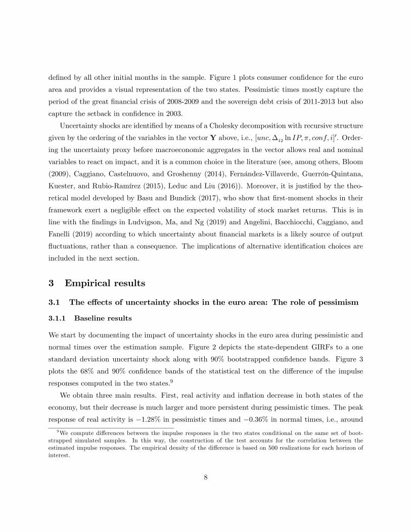
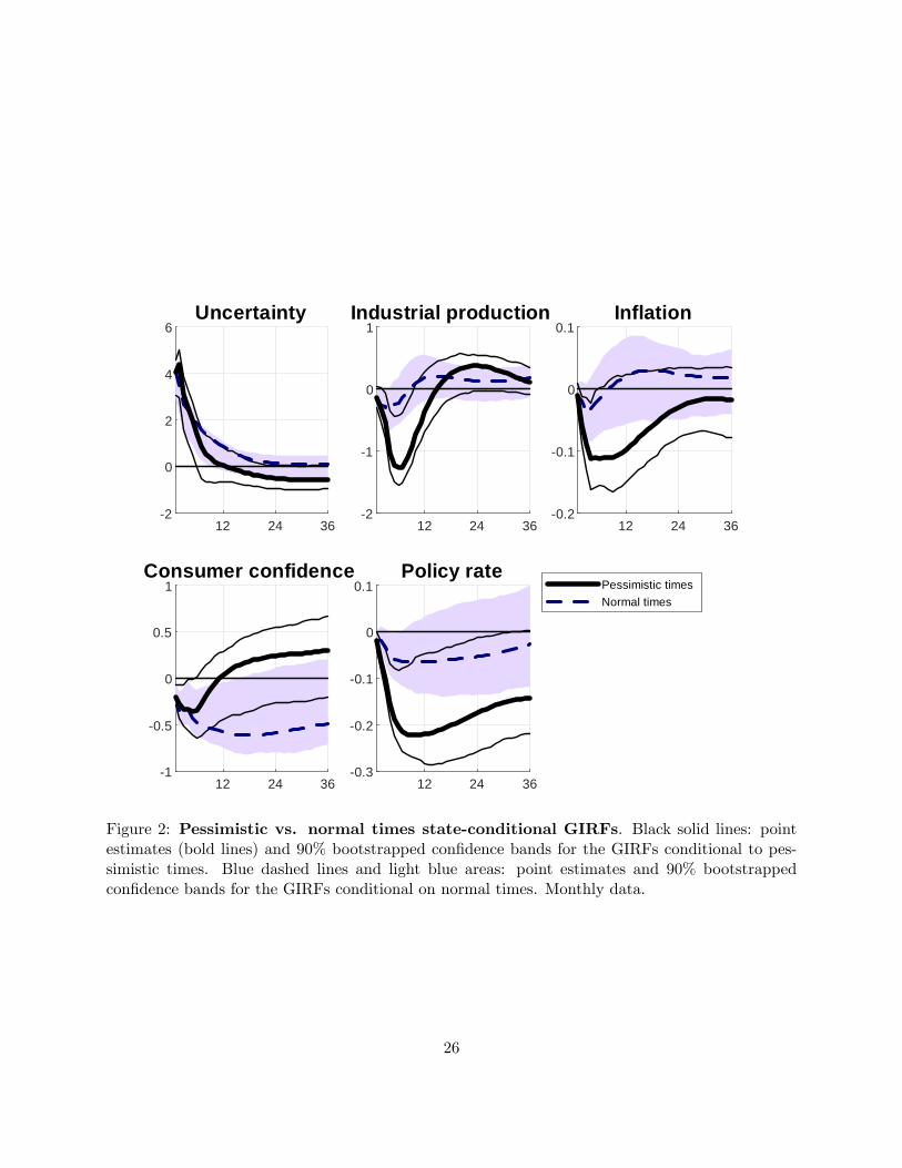
normal times over the estimation sample. Figure 2 depicts the state-dependent GIRFs to a one
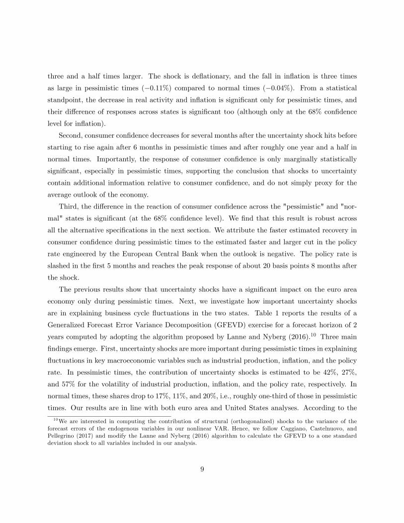
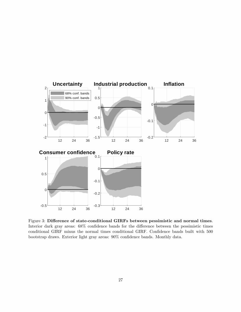
standard deviation uncertainty shock along with 90% bootstrapped confidence bands. Figure 3
plots the 68% and 90% confidence bands of the statistical test on the difference of the impulse
responses computed in the two states.9
We obtain three main results. First, real activity and inflation decrease in both states of the
economy, but their decrease is much larger and more persistent during pessimistic times. The peak
response of real activity is −1.28% in pessimistic times and −0.36% in normal times, i.e., around
9We compute differences between the impulse responses in the two states conditional on the same set of boot-strapped simulated samples. In this way, the construction of the test accounts for the correlation between theestimated impulse responses. The empirical density of the difference is based on 500 realizations for each horizon ofinterest.
8
three and a half times larger. The shock is deflationary, and the fall in inflation is three times
as large in pessimistic times (−0.11%) compared to normal times (−0.04%). From a statistical
standpoint, the decrease in real activity and inflation is significant only for pessimistic times, and
their difference of responses across states is significant too (although only at the 68% confidence
level for inflation).
Second, consumer confidence decreases for several months after the uncertainty shock hits before
starting to rise again after 6 months in pessimistic times and after roughly one year and a half in
normal times. Importantly, the response of consumer confidence is only marginally statistically
significant, especially in pessimistic times, supporting the conclusion that shocks to uncertainty
contain additional information relative to consumer confidence, and do not simply proxy for the
average outlook of the economy.
Third, the difference in the reaction of consumer confidence across the "pessimistic" and "nor-
mal" states is significant (at the 68% confidence level). We find that this result is robust across
all the alternative specifications in the next section. We attribute the faster estimated recovery in
consumer confidence during pessimistic times to the estimated faster and larger cut in the policy
rate engineered by the European Central Bank when the outlook is negative. The policy rate is
slashed in the first 5 months and reaches the peak response of about 20 basis points 8 months after
the shock.
The previous results show that uncertainty shocks have a significant impact on the euro area
economy only during pessimistic times. Next, we investigate how important uncertainty shocks
are in explaining business cycle fluctuations in the two states. Table 1 reports the results of a
Generalized Forecast Error Variance Decomposition (GFEVD) exercise for a forecast horizon of 2
years computed by adopting the algorithm proposed by Lanne and Nyberg (2016).10 Three main
findings emerge. First, uncertainty shocks are more important during pessimistic times in explaining
fluctuations in key macroeconomic variables such as industrial production, inflation, and the policy
rate. In pessimistic times, the contribution of uncertainty shocks is estimated to be 42%, 27%,
and 57% for the volatility of industrial production, inflation, and the policy rate, respectively. In
normal times, these shares drop to 17%, 11%, and 20%, i.e., roughly one-third of those in pessimistic
times. Our results are in line with both euro area and United States analyses. According to the
10We are interested in computing the contribution of structural (orthogonalized) shocks to the variance of theforecast errors of the endogenous variables in our nonlinear VAR. Hence, we follow Caggiano, Castelnuovo, andPellegrino (2017) and modify the Lanne and Nyberg (2016) algorithm to calculate the GFEVD to a one standarddeviation shock to all variables included in our analysis.
9
ECB Economic Bulletin (2016), uncertainty on average explains 20% of real GDP fluctuations in
the euro area. Jurado, Ludvigson, and Ng (2015) find that uncertainty shocks account for up to 29%
of the variation in United States industrial production at business cycle frequencies, and Caldara,
Fuentes-Albero, Gilchrist, and Zakrajšek (2016) find that uncertainty shocks explain between 20%
to 40% of the same. All these studies adopt linear VAR models. Our results imply that most of
the forecast error variance in economic aggregates that linear econometric methodologies attribute
to identified uncertainty shocks arise from the impact of these shocks during pessimistic times.
Second, the forecast error variance of the VSTOXX index is mainly explained by its own shock
in both states (89% in normal times and 92% in pessimistic times). This is consistent with the
findings by Ludvigson, Ma, and Ng (2019) and Angelini, Bacchiocchi, Caggiano, and Fanelli (2019)
according to which financial uncertainty is mostly an exogenous source of business cycle fluctuations.
Third, consumer confidence fluctuations are partially explained by uncertainty shocks, although
they explain only 10% of the volatility of consumer confidence during pessimistic times. This is
interesting as it suggests that during pessimistic times a larger part of the fluctuations in consumer
confidence reflects either autonomous shifts —which may be due to both ‘animal spirits’or funda-
mental information, or ‘news’, about the future state of the economy available to consumers and
not summarized by other measurable variables (Barsky and Sims (2012)) —or a reaction to other
shocks. Consistently with this interpretation, we find that consumer confidence (monetary policy)
shocks explain 33% (3.5%) of the business cycle fluctuations in confidence in pessimistic times, and
27% (2.2%) in normal times.
What explains the result of a severe impact of an uncertainty shock conditional on a pessimistic
outlook? Heightened uncertainty translates, from the point of view of consumers and businesses,
into a higher chance of more extreme outcomes, i.e., a higher chance of large upside or downside
risk, for a given average outlook. Consumers are risk-averse: they would prefer a lower income with
certainty, compared to an environment with a chance of very negative outcomes - such as becoming
unemployed - even if they were guaranteed that their expected lifetime income would be identical
in the two environments. Businesses, when faced with more uncertainty about future demand, may
find optimal to postpone investments.
At times of low prospects for future economic activity, an increase in the dispersion of future
outcomes may have a larger impact on the economy: many more consumers, for example, may be
closer to a worst-case scenario where they lose any income stream completely, and may optimally
choose to change their behavior because of the increase in risk —even if there is an equally likely
10
probability that the economy will rebound fast and demand growth will raise incomes. The same
may be true for firms: with a very negative outlook, the same increase in uncertainty can — for
example —dramatically raise the probability of bankruptcy for many firms, leading to a sharper
change in behavior than what would be observed in normal times with a less extreme outlook (this
intuition is formalized in Fajgelbaum, Schaal, and Taschereau-Dumouchel (2014) and Cacciatore
and Ravenna (2020), among others).
3.1.2 Alternative Hypotheses on the Impact of Uncertainty Shocks
In this section we study alternative specifications to discuss further findings on the role of pessimism
in the transmission mechanism of uncertainty shocks. We explore the transmission of global un-
certainty shocks, the relevance of survey-derived measures of expectations dispersion, the specific
importance of consumer confidence, and the implications of an alternative interpretation of pes-
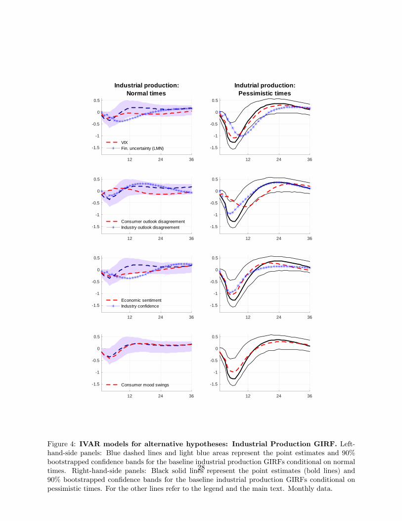
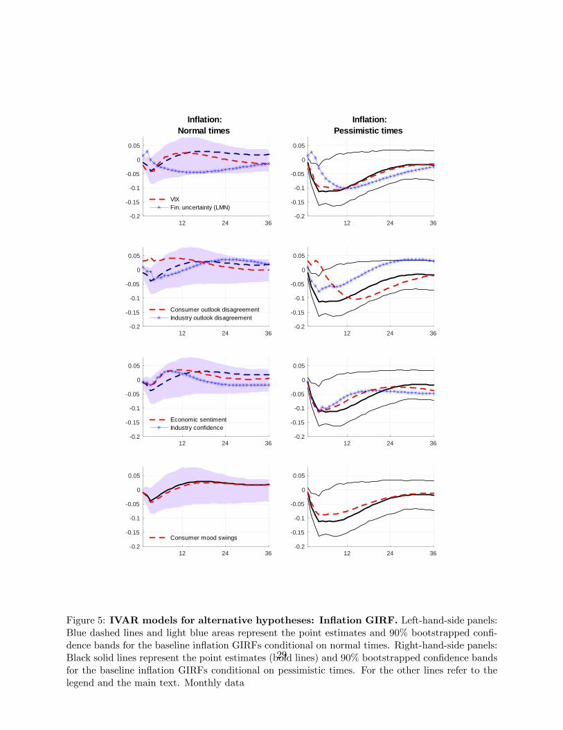
simism based on mood swings. The findings are shown in Figures 4 and 5, for real activity and
inflation, respectively.
Non-European financial uncertainty indicators. In our baseline analysis, we use the
VSTOXX volatility index, as an index of European financial uncertainty. However, most of its
spikes coincide with global, or non-European, events, such as Worldcom and Enron United States
financial scandals in 2002, Gulf War II in 2003, and the Global Financial Crisis (see the first panel
of Figure A1 in the Appendix). We assess whether the spillover effects of global uncertainty shocks
to the euro area depend on the local, euro area level of confidence. To this end, we re-estimate the
IVAR employing the United States VIX index in place of our european uncertainty indicator.
As an alternative indicator, we also use the Ludvigson, Ma, and Ng’s (LMN, 2019) United States
financial uncertainty index in place of the VIX. The index is a computed by adopting the same
data-rich methodology proposed in Jurado, Ludvigson, and Ng (2015), i.e., it is the average of the
conditional volatilities of the unforecastable components of a large dataset of financial variables.
The findings in the top panels of Figures 4 and 5 document that global financial uncertainty shocks
have spillover effects in the euro area that also depend on the european confidence level. The results
are very similar to the baseline ones. The key difference is that the LMN financial uncertainty index
implies larger and more persistent real effects in both states. Large co-movements across the main
global trading areas level of output may explain this result, although the correlation of the VSTOXX
with the VIX and the LMN measure is respectively 0.86 and 0.69.
European uncertainty indicators based on survey-derived measures of expectations
11

dispersion. Provided that our IVAR makes use of a survey-based measure of consumer confidence,
it is interesting to verify whether shocks to survey-based indicators of expectations dispersion, or
"disagreement", also affect real activity and inflation in a state-dependent manner according to the
level of consumer confidence. We hence use measures of survey-based disagreement in place of our
baseline uncertainty indicator. This is close in spirit to Bachmann, Elstner, and Sims (2013) who
use survey expectations data from both Germany and the United States to construct empirical
proxies for time-varying business-level uncertainty.11
To construct a consumer disagreement index, we exploit the dispersion of responses to the
following forward-looking survey question12:
How do you expect the financial position of your household to change over the next 12
months?
++ "get a lot better"; + "get a little better"; = "stay the same"; − "get a little worse";−− ’get a lot worse’; NA "don’t know".
In accordance with the construction of the consumer confidence level index, we assign the
values 1, 0.5, 0, −0.5 and −1 to each of those categories (see european Commission’s (2020) survey
user guide, p. 14). Let, without loss of generality, the weighted fraction of consumers with a
very positive outlook at time t be Frac++t . We compute the consumer disagreement index as the
standard deviation of response values weighted with the respective fractions, i.e.:
EDISPcons. =
√√√√ Frac++t · (1−mean)2 + Frac+t · (0.5−mean)2
+Frac−t · (−0.5−mean)2 + Frac−−t · (−1−mean)2,
where:
mean = 1 · Frac++t + 0.5 · Frac+
t − 0.5 · Frac−t − 1 · Frac−−t
For the equivalent index of industrial firm responses, we consider the following four questions
in the industry subsector of the european Commission’s business survey:
1. Do you consider your current overall order books to be:/
11Bomberger (1996) validates the use of survey-based measures of dispersion across forecasters as proxies for theuncertainty surrounding the mean forecast. Specifically, he shows that the conditional variance of forecast errors froman ARCH model is positively related to the disagreement among forecasters at the time of the forecast.12The following is question 2 of the European Commission (2020) Consumer Survey, one of the questions at the
basis of the Consumer Confidence Index we adopt.
12
2. Do you consider your current export order books to be:/
3. Do you consider your current stock of finished products to be:
+ "more than suffi cient/above normal”; = “suffi cient/normal for the season”; − “not suffi -cient/below normal”; NA “refused/not applicable”?
4. How do you expect your production to develop over the next 3 months?
+ “increase”; = “remain unchanged”; − “decrease".
Letting again Frac+t (Frac
−t ) denote the weighted fraction of firms in the cross-section with
“increase”(“decrease”) responses at time t, the EDISP dispersion indicators are then computed
for each question as in Meinen and Röhe (2017):
EDISPind.,i =
√Frac+
t + Frac−t −(Frac+
t + Frac−t)2
; i = 1, 2, 3, 4.
We compute an unweighted average across the questions which we refer to as “industry outlook
disagreement”. The time series is displayed in Figure A4, together with all uncertainty indices used
throughout the paper. As the panels in the second row of Figures 4 and 5 document, disagreement
shocks also feature a confidence-dependent transmission mechanism. While shocks to industry
outlook disagreement have effects similar to our baseline ones, consumer disagreement shocks have
milder effects on real activity in both states and have mild inflationary effects in the short run.
Economic sentiment and industry confidence. In our baseline, we use the Consumer
Confidence Index provided by the european Commission as an indicator of expectations for the
economic outlook. We now ask how confidence affects the impact of uncertainty shocks when
broadening the measure of confidence to include producers’ expectations. We introduce in the
IVAR the Economic Sentiment Indicator, which is a composite of indices across consumers and
producers in 5 sectors. We also consider its industry component alone. The latter covers firms in
the manufacturing sector (2-digit NACE codes 10 to 33), which allows us to have a direct forward-
looking equivalent to the industrial production series used in the VAR. The Appendix reports all
the economic outlooks series we use and the third row of panels of Figures 4 and 5 reports novel
findings. The IVAR results are similar to the baseline ones, with two key differences. First, industry
confidence now implies a more persistent drop in real activity in normal times with the peak drop
reached after a year. Second, both economic sentiments and industry confidence are only mildly
deflationary in the short run.
13
Definition of pessimistic times related to mood swings. In our baseline analysis, we
use the level of consumer confidence to define our pessimistic-times state. The idea behind this
choice is that a low value in the index reflects pessimism, i.e., a negative outlook for the future
of the economy. However, one can argue that pessimism can also be reflected by sudden negative
changes in consumer confidence that are unrelated to the level of the series. In fact, as Figure 1
documents, our pessimistic-times state includes both phases with plummeting consumer confidence
and recovering phases. In order to investigate this alternative interpretation of pessimism based on
mood swings, we classify an initial month to the pessimistic times state whenever the cumulative
change in the last six months of the Consumer Confidence Index is in its bottom 20%. The Appen-
dix reports the visual representation of this alternative pessimistic-times state. Now, pessimistic
times only include phases of negative mood swings and more episodes (also outside recessions) are
classified into this state. The results —documented in the fourth row of panels of Figures 4 and
5 —are very similar to baseline ones, the only difference being that now uncertainty shocks have
milder effects under this alternative interpretation of pessimistic times.
Overall, we interpret the findings in Figures 4 and 5 as strongly supporting our baseline result,
also when exploring alternative connected hypotheses and data measures.
3.1.3 Alternative Econometric Specifications
Before using our baseline results to predict the impact of the COVID-19 induced uncertainty shock,
we check that they are robust to perturbations regarding both the control for financial variables, the
identification approach adopted, and the definition of pessimistic times. Results for both industrial
production and inflation are summarized in Figure 6.
Control for financial variables. Our baseline VAR does not model any financial variable.
However, financial stress indicators —such as credit spreads —can be relevant to the econometric
specification for at least three reasons. First, it is well known that credit spreads have large
predictive power for both United States and euro area real activity (see Gilchrist and Zakrajšek
(2012) and Gilchrist and Mojon (2018), respectively). Second, as advocated by recent studies,
financial frictions and credit spreads are important for the transmission of uncertainty shocks
(Alfaro, Bloom, and Lin (2018), Gilchrist, Sim, and Zakrajšek (2014) and Arellano, Bai, and Kehoe
(2019)). A recent paper by Görtz, Tsoukalas, and Zanetti (2016) shows that movements in credit
spreads are also relevant for the propagation of news shocks. Third, thanks to the consideration of
credit spreads we can capture the effects of unconventional monetary policy in the euro area since
14

it operated at the long-term of the yield curve.
We alternatively add two bond spread indicators to our baseline IVAR and order them just after
the VSTOXX uncertainty measure.13 First, we use a high yield spread that tracks the performance
of euro-denominated below-investment-grade corporate debt publicly issued in the euro markets
with respect to a portfolio of Treasury bonds.14 Second, we use the Gilchrist and Mojon’s (2018)
credit spread of euro area non-financial corporations. The authors follow the methodology of
Gilchrist and Zakrajšek (2012) and use individual bond level data to construct bond-specific credit
spreads, which are then averaged to obtain credit spread indices at the country level. These credit
spread indices are defined as the difference between the corporate bond yield and the country-
specific sovereign bond yield. By aggregating this information across countries, they construct credit
spreads for the euro area as a whole.15 As Figure 6 documents, controlling for financial variables
does not affect our main results: the impulse responses under these alternative specifications of our
IVAR are within the baseline results confidence bands.
Identification via external instrument: A Proxy Strucural IVAR. In our baseline,
we use a recursive (Cholesky) strategy to identify uncertainty shocks. Our recursive identification
allows for an immediate impact of uncertainty shocks but treats financial uncertainty as exogenous
to the business cycle. To document the robustness of our main results, we adopt an alternative
identification scheme, via external instruments, adopted in Proxy Structural VARs (see Stock and
Watson (2012), Mertens and Ravn (2013), Mertens and Ravn (2014), Gertler and Karadi (2015),
Piffer and Podstawski (2018)). We follow Piffer and Podstawski (2018), who propose an instrument
to identify uncertainty shocks within proxy SVARs. Their instrument equals the percentage varia-
tions in the price of gold —which is perceived as a safe haven asset —around events associated with
unexpected changes in uncertainty. The Appendix shows how to apply the external instrument
identification to IVAR models. The gold instrument is used in an IVAR that features the VXO
13The use of a Cholesky decomposition does not allow us to easily disentangle uncertainty from financial shocksprovided that both variables are fast-moving and are contemporaneously correlated (see Caldara, Fuentes-Albero,Gilchrist, and Zakrajšek (2016)). We order the credit spread as the second variable so as to allow it to contempora-neously react to uncertainty shocks. In this way, we can account for both their influence on real activity and theircrucial role in the transmission of uncertainty shocks.14Our credit spread measure is the ICE/BofA Euro High Yield Index Spread (source: Federal Reserve Bank of St.
Louis).15The credit spread indicators proposed by Gilchrist and Mojon (2018) are monthly updated and available
at the link https://publications.banque-france.fr/en/economic-and-financial-publications-working-papers/credit-risk-euro-area. We use the variable spr_nfc_dom_ea, which refers to the euro area credit spread for non-financialcorporations.
15

as the uncertainty measure, as in Piffer and Podstawski (2018).16 Figure 6 shows that our main
results are robust to the use of this alternative external instrument identification scheme. Impulse
responses overall lie within the baseline estimation confidence bands except for the short-run re-
sponse of inflation, which increases after an uncertainty shock, and the short-run response of real
activity, which now features a bigger drop in normal times.
Alternative thresholds for the definition of pessimistic times. In our baseline, we use
the bottom quintile of the historical distribution of consumer confidence to define our pessimistic-
times state. We check that our results are not driven by this definition by alternatively using either
the bottom decile or the bottom tertile as the relevant thresholds. Figure 6 documents that results
are robust to this perturbation.
Our main results are also robust to the use of alternative lag orders (3 and 6).
3.2 The uncertainty-channel of the COVID-19 shock
We use the baseline IVAR results to predict the possible effects of the COVID-19 shock via its
uncertainty channel. COVID-19 caused enormous increases in financial uncertainty in the first half
of 2020. Uncertainty measures have been surging since late February 2020, when the first cases in
the euro area not directly related to China were detected in Italy. During March the index saw its
largest increase, in the period when the World Health Organization (WHO) declared a pandemic
emergency on March 11. In the next few days, most euro area countries closed their schools and
borders (e.g., Germany on March 13 and 15, respectively) and adopted a lockdown (Germany on
March 22, the same date when Italy implemented the strictest measures for its lockdown already
started on March 9). Only in late April 2020, did the euro area’s countries have been relax their
restrictions.
The April release of the european Commission Consumer Confidence Indicator signaled a con-
fidence level approaching the level reached during the 2008-2009 financial crisis. In the previous
Section, we computed the effects of a typical uncertainty shock occurring during pessimistic times
and found that it has stronger effects than during normal times. The peak reaction of real activity
16The instrument is available on Michele Piffer’s webpage (https://sites.google.com/site/michelepiffereconomics/).For our sample period, the instrument is associated with an F statistic equal to 8.17. Our first-stage regressioncoeffi cient is 155.82 which is close to Piffer and Podstawski’s (2018, Table 2) one of 166.40, notwithstanding thedifferent sample considered. Unlike Piffer and Podstawski (2018), we do not use a set-identified Proxy SVAR thatidentifies uncertainty and news shocks jointly, but rather use their instrument to exactly identify the impulse responsesassociated with uncertainty shocks, an approach common in the Proxy SVAR literature. Piffer and Podstawski (2018,Figure H18) shows that the two approaches produce similar results for their analysis.
16
is roughly 3.5 times stronger during pessimistic times than normal times. We now simulate the
effects of the COVID-19 related surge in uncertainty by using the pessimistic-times state of our
estimated IVAR.
The use of a nonlinear VAR is ideal to answer our COVID-19 related question because it can
account for the unusual circumstances the euro area economy is currently facing in terms of both
uncertainty and consumer confidence. Moreover, the current values of consumer confidence and
uncertainty do not represent outliers in our sample, something that reassures us of the information
carried by our IVAR for the assessment of the uncertainty-channel of the COVID-19 shock.
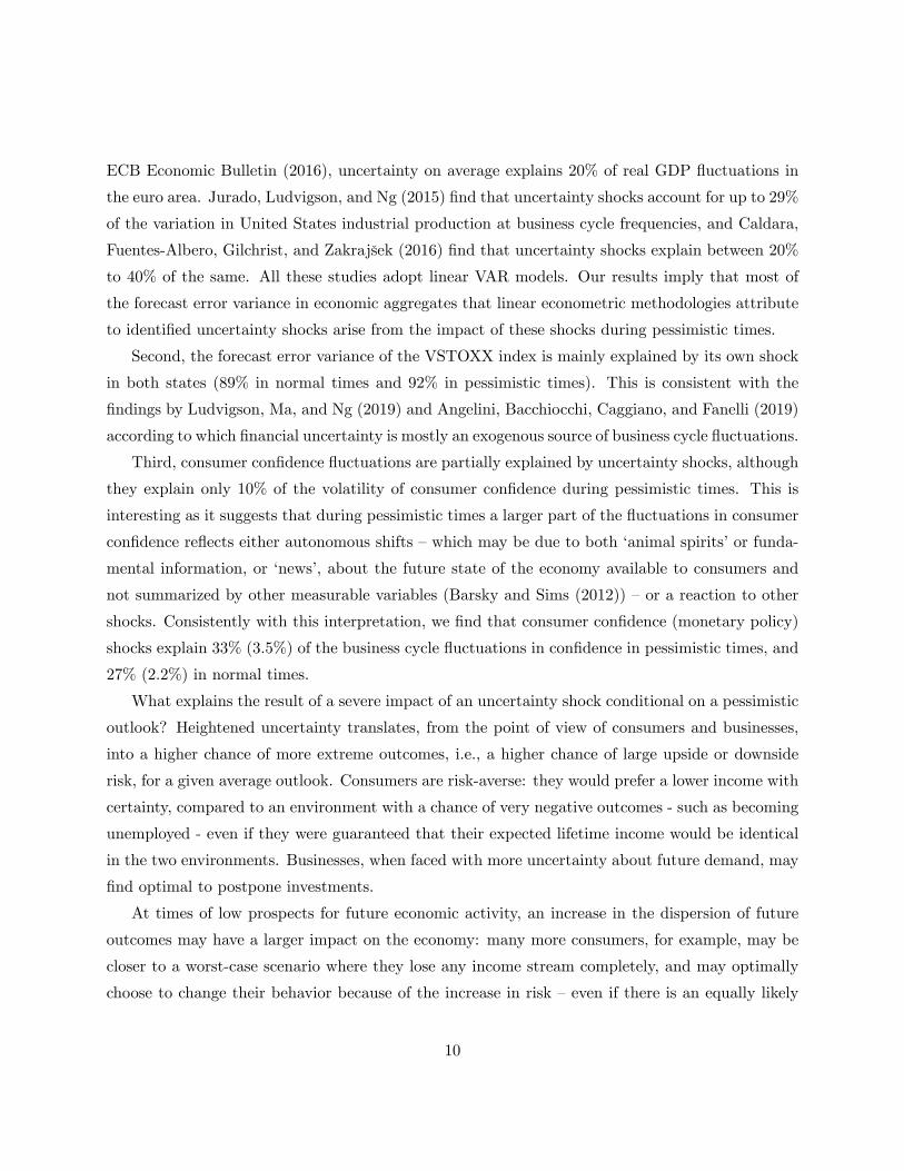
According to our estimated IVAR, the unexpected rise in the level of the VSTOXX measure of
uncertainty from February 2020 to March 2020 corresponds to roughly a ten standard deviation
shock. The black line in Figure 7 plots the effects of such an uncertainty shock during the average
pessimistic state according to our estimated IVAR.17 As Table 2 clarifies, industrial production ex-
periences a year-over-year peak loss of 15.41% peaking after 7 months from the shock, in September
2020, and subsequently it recovers with a rebound to pre-crisis levels predicted to happen in May
2021. Given that our measure of industrial production is 2.8 times more volatile than the corre-
sponding measure of GDP, a back-of-the-envelope calculation would translate the IVAR prediction
for industrial production into a year-over-year fall in GDP of roughly 4.3% at peak. Inflation’s
year-over-year peak decrease is predicted to be −1.35% in August 2020.
What if the COVID-19 related uncertainty shock propagated in a way different from the past
euro area experience? In performing the previous exercise, we considered the persistence of a typical
uncertainty shock as estimated by our IVAR on past data. Two alternative scenarios are plausible in
the COVID-19 pandemic. We first assume that uncertainty can go back to normal levels much more
slowly in the current situation than in the past, given that the persisting uncertainty in delivering
a vaccine could span several months. Alternatively, a second unexpected spike in uncertainty may
occur following a new wave of the pandemic in the coming 6 to 9 months. In order to construct
these two possible scenarios, we compute GIRFs by feeding a sequence of shocks. We generalize
the GIRF definition in equation (2) with the following:
GIRFY,t(h, δ,$t−1) = E [Yt+h | δ,$t−1]− E [Yt+h |$t−1] , h = 0, 1, . . . ,H, (3)
17 Imposing a shock as large as 10 standard deviations causes our IVAR pessimistic times’response - which is basedon an average of 50 initial quarters responses - to discard 5 particularly extreme initial histories which would lead toan explosive response. This implies that the estimated impact of the COVID-related uncertainty shock we report isconservative. However, our pessimistic times’response to a one standard deviation shock at the basis of Figure 2 didnot discard any initial quarter.
17
where now δ is a vector including several unexpected shocks hitting at different times, or δ = [δt, δt+1,..., δt+H ].
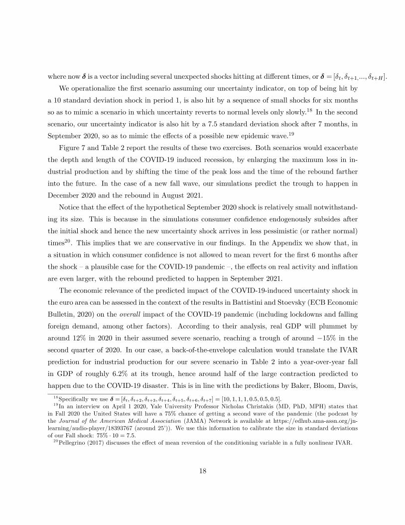
We operationalize the first scenario assuming our uncertainty indicator, on top of being hit by
a 10 standard deviation shock in period 1, is also hit by a sequence of small shocks for six months
so as to mimic a scenario in which uncertainty reverts to normal levels only slowly.18 In the second
scenario, our uncertainty indicator is also hit by a 7.5 standard deviation shock after 7 months, in
September 2020, so as to mimic the effects of a possible new epidemic wave.19
Figure 7 and Table 2 report the results of these two exercises. Both scenarios would exacerbate
the depth and length of the COVID-19 induced recession, by enlarging the maximum loss in in-
dustrial production and by shifting the time of the peak loss and the time of the rebound farther
into the future. In the case of a new fall wave, our simulations predict the trough to happen in
December 2020 and the rebound in August 2021.
Notice that the effect of the hypothetical September 2020 shock is relatively small notwithstand-
ing its size. This is because in the simulations consumer confidence endogenously subsides after
the initial shock and hence the new uncertainty shock arrives in less pessimistic (or rather normal)
times20. This implies that we are conservative in our findings. In the Appendix we show that, in
a situation in which consumer confidence is not allowed to mean revert for the first 6 months after
the shock —a plausible case for the COVID-19 pandemic —, the effects on real activity and inflation
are even larger, with the rebound predicted to happen in September 2021.
The economic relevance of the predicted impact of the COVID-19-induced uncertainty shock in
the euro area can be assessed in the context of the results in Battistini and Stoevsky (ECB Economic
Bulletin, 2020) on the overall impact of the COVID-19 pandemic (including lockdowns and falling
foreign demand, among other factors). According to their analysis, real GDP will plummet by
around 12% in 2020 in their assumed severe scenario, reaching a trough of around −15% in the
second quarter of 2020. In our case, a back-of-the-envelope calculation would translate the IVAR
prediction for industrial production for our severe scenario in Table 2 into a year-over-year fall
in GDP of roughly 6.2% at its trough, hence around half of the large contraction predicted to
happen due to the COVID-19 disaster. This is in line with the predictions by Baker, Bloom, Davis,
18Specifically we use δ = [δt, δt+2, δt+3, δt+4, δt+5, δt+6, δt+7] = [10, 1, 1, 1, 0.5, 0.5, 0.5].19 In an interview on April 1 2020, Yale University Professor Nicholas Christakis (MD, PhD, MPH) states that
in Fall 2020 the United States will have a 75% chance of getting a second wave of the pandemic (the podcast bythe Journal of the American Medical Association (JAMA) Network is available at https://edhub.ama-assn.org/jn-learning/audio-player/18393767 (around 25’)). We use this information to calibrate the size in standard deviationsof our Fall shock: 75% · 10 = 7.5.20Pellegrino (2017) discusses the effect of mean reversion of the conditioning variable in a fully nonlinear IVAR.
18
and Terry (2020) for the United States. According to their estimates, around half of the total
contraction induced by the COVID-19 disaster will be due to the COVID-19-induced uncertainty
shock.
4 Conclusion
We analyze the impact of the COVID-19 shock via its uncertainty channel using an IVAR model for
the euro area. The COVID-19 shock can be interpreted as a rare natural disaster shock that, because
of its long-term consequences, also affects economic uncertainty, as documented by Ludvigson, Ma,
and Ng (2020) and Baker, Bloom, Davis, and Terry (2020). Like the latter studies, we rely on
past historical data to predict the macroeconomic impact of the COVID-19 induced uncertainty
shock, and as such appropriate caveats apply to our analysis. However, to try mitigating them,
we considered alternative scenarios accounting for a potentially different propagation of this huge
uncertainty shock.
Our results suggest that the impact of an uncertainty shock in the euro area is highly state-
dependent, and varies according to the expectations for the economic outlook as measured by
several confidence survey-measures. Using the estimated IVAR model, we assess that the rebound
after the COVID-19 epidemics will be slow and painful - even if the impact occurred only through
the massive increase in uncertainty. This is caused by the uncertainty shock hitting the euro area
economy at a time of a severely negative economic outlook. Even when lockdowns will gradually
be relaxed, there will still be a drag on the euro area economy given by the heightened level of
uncertainty about the future.
The current experience is unique, in that measures of uncertainty registered surges in both the
United States and the euro area equal to several standard deviations, and measures of economic
sentiment simultaneously hit their record bottom. If the uncertainty-channel alone can explain
a substantial share of the overall cost of the COVID-19 disaster shock, policymakers ought to
seriously consider enacting clear policies aimed not only at boosting confidence in the outlook, but
specifically aimed at resolving the uncertainty, by providing to the public contingent scenarios and
policies ready to be adopted if the worst-case outcomes materialize.
19
References
Alessandri, P., and H. Mumtaz (2019): “Financial Regimes and Uncertainty Shocks,”Journalof Monetary Economics, 101, 31—46.
Alfaro, I., N. Bloom, and X. Lin (2018): “The Finance Uncertainty Multiplier,”NBER Work-ing Paper No 24571.
Andreasen, M., G. Caggiano, E. Castelnuovo, and G. Pellegrino (2020): “Uncertaintyshocks and Real Activity in Booms and Busts: A Structural Interpretation,”Aarhus University,Monash University, and University of Melbourne, in progress, preliminary draft available athttps://sites.google.com/site/giovannipellegrinopg/home/research.
Andreasen, M. M., J. Fernández-Villaverde, and J. F. Rubio-Ramírez (2017): “Thepruned state-space system for non-linear DSGE models: Theory and empirical applications,”The Review of Economic Studies, 85(1), 1—49.
Angelini, G., E. Bacchiocchi, G. Caggiano, and L. Fanelli (2019): “Uncertainty acrossvolatility regimes,”Journal of Applied Econometrics, 34(3), 437—455.
Arellano, C., Y. Bai, and P. J. Kehoe (2019): “Financial Frictions and Fluctuations inVolatility,”Journal of Political Economy, 127(5), 2049—2103.
Bachmann, R., S. Elstner, and E. Sims (2013): “Uncertainty and Economic Activity: Evidencefrom Business Survey Data,”American Economic Journal: Macroeconomics, 5(2), 217—249.
Baker, S., N. Bloom, and S. J. Davis (2016): “Measuring Economic Policy Uncertainty,”Quarterly Journal of Economics, 131(4), 1539—1636.
Baker, S. R., N. Bloom, S. J. Davis, and S. J. Terry (2020): “Covid-induced economicuncertainty,”Discussion paper, National Bureau of Economic Research.
Barsky, R. B., and E. R. Sims (2012): “Information, animal spirits, and the meaning of inno-vations in consumer confidence,”American Economic Review, 102(4), 1343—77.
Basu, S., and B. Bundick (2017): “Uncertainty Shocks in a Model of Effective Demand,”Econo-metrica, 85(3), 937—958.
Bernanke, B. S. (1983): “Irreversibility, Uncertainty, and Cyclical Investment,”Quarterly Jour-nal of Economics, 98(1), 85—106.
Bloom, N. (2009): “The Impact of Uncertainty Shocks,”Econometrica, 77(3), 623—685.
Bomberger, W. A. (1996): “Disagreement as a Measure of Uncertainty,” Journal of Money,Credit and Banking, 28(3), 381—392.
Caballero, R. (1990): “Consumption Puzzles and Precautionary Savings,”Journal of MonetaryEconomics, 25, 113—136.
Cacciatore, M., and F. Ravenna (2020): “Uncertainty, Wages, and the Business Cycle,”HECMontreal, mimeo.
20
Caggiano, G., E. Castelnuovo, and J. M. Figueres (2020): “Economic Policy UncertaintySpillovers in Booms and Busts,”Oxford Bulletin of Economics and Statistics, 82(1), 125—155.
Caggiano, G., E. Castelnuovo, and N. Groshenny (2014): “Uncertainty Shocks and Un-employment Dynamics: An Analysis of Post-WWII U.S. Recessions,”Journal of Monetary Eco-nomics, 67, 78—92.
Caggiano, G., E. Castelnuovo, and R. Kima (2020): “The global effects of Covid-19-induced uncertainty,” Monash University and University of Melbourne, available athttps://sites.google.com/site/efremcastelnuovo/.
Caggiano, G., E. Castelnuovo, and G. Pellegrino (2017): “Estimating the Real Effects ofUncertainty Shocks at the Zero Lower Bound,”European Economic Review, 100, 257—272.
Caldara, D., C. Fuentes-Albero, S. Gilchrist, and E. Zakrajek (2016): “The Macroeco-nomic Impact of Financial and Uncertainty Shocks,”European Economic Review, 88, 185—207.
Castelnuovo, E. (2016): “Modest Macroeconomic Effects of Monetary Policy Shocks During theGreat Moderation: An Alternative Interpretation,”Journal of Macroeconomics, 47, 300—314.
Chatterjee, P. (2018): “Asymmetric Impact of Uncertainty in Recessions - Are Emerging Coun-tries More Vulnerable?,”Studies in Nonlinear Dynamics and Econometrics, forthcoming.
Christiano, L. J., M. Eichenbaum, and C. Evans (1999): “Monetary Policy Shocks: WhatHave We Learned and to What End?,” In: J.B. Taylor and M. Woodford (eds.): Handbook ofMacroeconomics, Elsevier Science, 65—148.
ECB (2016): “The impact of uncertainty on activity in the euro area,”Economic Bulletin, Issue8.
(2020): “Alternative scenarios for the impact of the COVID-19 pandemic on economicactivity in the euro area,” Economic Bulletin, Issue 3. May 14. Study prepared by NiccolòBattistini and Grigor Stoevsky.
EuropeanCommission (2020a): “Flash Consumer Confidence Indicator for EU and Euro Area,Press Release, 23 April 2020,”Discussion paper.
(2020b): “The Joint Harmonised EU Programme of Business and ConsumerSurveys: User Guide, February 2020,” Discussion paper, Directorate-General for Eco-nomic and Financial Affairs, https://ec.europa.eu/info/files/user-guide-joint-harmonised-eu-programme-business-and-consumer-surveysen.
Fajgelbaum, P., E. Schaal, and M. Taschereau-Dumouchel (2014): “Uncertainty Traps,”Working Paper 19973, National Bureau of Economic Research.
Fernández-Villaverde, J., P. Guerrón-Quintana, K. Kuester, and J. Rubio-Ramírez(2015): “Fiscal Volatility Shocks and Economic Activity,”American Economic Review, 105(11),3352—84.
Gertler, M., and P. Karadi (2015): “Monetary Policy Surprises, Credit Costs, and EconomicActivity,”American Economic Journal: Macroeconomics, 7(1), 44—76.
21
Gilchrist, S., and B. Mojon (2018): “Credit risk in the euro area,” The Economic Journal,128(608), 118—158.
Gilchrist, S., J. W. Sim, and E. Zakrajek (2014): “Uncertainty, financial frictions, and invest-ment dynamics,”Discussion paper, National Bureau of Economic Research.
Gilchrist, S., and E. Zakrajek (2012): “Credit Spreads and Business Cycle Fluctuations,”American Economic Review, 102(4), 1692—1720.
Görtz, C., J. D. Tsoukalas, and F. Zanetti (2016): “News Shocks under Financial Frictions,”Working Paper 2016 15, Business School - Economics, University of Glasgow.
Jurado, K., S. C. Ludvigson, and S. Ng (2015): “Measuring Uncertainty,”American EconomicReview, 105(3), 1177—1216.
Kilian, L., and R. Vigfusson (2011): “Are the Responses of the U.S. Economy Asymmetric inEnergy Price Increases and Decreases?,”Quantitative Economics, 2, 419—453.
Koop, G., M. Pesaran, and S. Potter (1996): “Impulse response analysis in nonlinear multi-variate models,”Journal of Econometrics, 74(1), 119—147.
Lanne, M., and H. Nyberg (2016): “Generalised Forecast Error Variance Decomposition for Linearand Nonlinear Multivariate Models,”Oxford Bulletin of Economics and Statistics, 78, 595—603.
Leduc, S., and Z. Liu (2016): “Uncertainty Shocks are Aggregate Demand Shocks,” Journal ofMonetary Economics, 82, 20—35.
(2020): “The Uncertainty Channel of the Coronavirus,”FRBSF Economic Letter, 2020(07),1—05.
Lhuissier, S., and F. Tripier (2019): “Regime-Dependent Effects of Uncertainty Shocks: A Struc-tural Interpretation,”Banque de France Working Paper No. 714.
Ludvigson, S. C., S. Ma, and S. Ng (2019): “Uncertainty and Business Cycles: Exogenous Impulseor Endogenous Response?,”American Economic Journal: Macroeconomics, forthcoming.
Ludvigson, S. C., S. Ma, and S. Ng (2020): “Covid19 and the Macroeconomic Effects of CostlyDisasters,”Working Paper 26987, National Bureau of Economic Research.
Meinen, P., and O. Röhe (2017): “On measuring uncertainty and its impact on investment: Cross-country evidence from the euro area,”European Economic Review, 92(C), 161—179.
Mertens, K., and M. O. Ravn (2013): “The Dynamic Effecs of Personal and Corporate IncomeTax Changes in the United States,”American Economic Review, 103(4), 1212—1247.
(2014): “A Reconciliation of SVAR and Narrative Estimates of Tax Multipliers,”Journal ofMonetary Economics, 68, S1—S19.
Mumtaz, H., and F. Zanetti (2013): “The Impact of the Volatility of Monetary Policy Shocks,”Journal of Money, Credit and Banking, 45(4), 535—558.
Pellegrino, G. (2017): “Uncertainty and Monetary Policy in the US: A Journey into Non-LinearTerritory,”Melbourne Institute Working Paper No. 6/17.
22
(2018): “Uncertainty and the Real Effects of Monetary Policy Shocks in the Euro Area,”Economics Letters, 162, 177—181.
Pesaran, H. M., and Y. Shin (1998): “Generalized Impulse Response Analysis in Linear Multi-variate Models,”Economics Letters, 58, 17—29.
Piffer, M., and M. Podstawski (2018): “Identifying uncertainty shocks using the price of gold,”Economic Journal, 128(616), 3266—3284.
Smets, F., and R. Wouters (2003): “An Estimated Dynamic Stochastic General EquilibriumModel of the Euro Area,”Journal of the European Economic Association, 1, 1123—1175.
Stock, J. H., andM. W. Watson (2012): “Disentangling the Channels of the 2007-2009 Recession,”Brookings Papers on Economic Activity, Spring, 81—135.
23
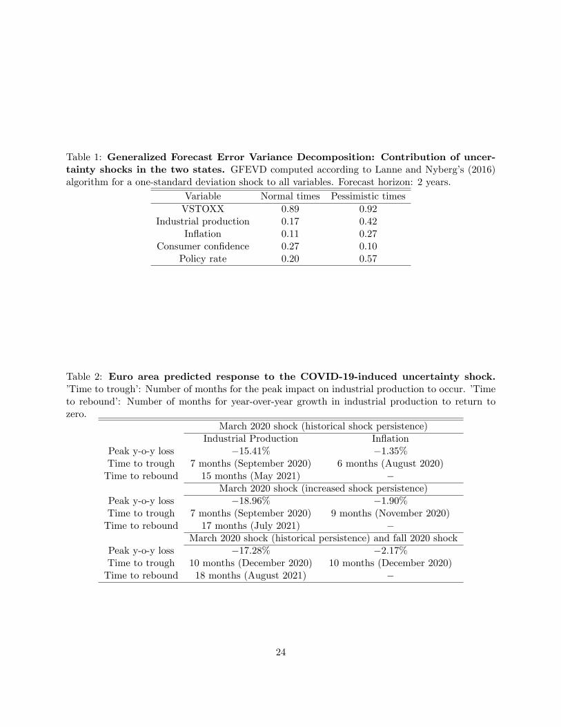
Table 1: Generalized Forecast Error Variance Decomposition: Contribution of uncer-tainty shocks in the two states. GFEVD computed according to Lanne and Nyberg’s (2016)algorithm for a one-standard deviation shock to all variables. Forecast horizon: 2 years.
Variable Normal times Pessimistic timesVSTOXX 0.89 0.92
Industrial production 0.17 0.42Inflation 0.11 0.27
Consumer confidence 0.27 0.10Policy rate 0.20 0.57
Table 2: Euro area predicted response to the COVID-19-induced uncertainty shock.’Time to trough’: Number of months for the peak impact on industrial production to occur. ’Timeto rebound’: Number of months for year-over-year growth in industrial production to return tozero.
March 2020 shock (historical shock persistence)Industrial Production Inflation
Peak y-o-y loss −15.41% −1.35%Time to trough 7 months (September 2020) 6 months (August 2020)Time to rebound 15 months (May 2021) −
March 2020 shock (increased shock persistence)Peak y-o-y loss −18.96% −1.90%Time to trough 7 months (September 2020) 9 months (November 2020)Time to rebound 17 months (July 2021) −
March 2020 shock (historical persistence) and fall 2020 shockPeak y-o-y loss −17.28% −2.17%Time to trough 10 months (December 2020) 10 months (December 2020)Time to rebound 18 months (August 2021) −
24
Consumer confidence
2000 2004 2008 2012 2016 2020
10
5
0
5
Pessimistic times
Figure 1: European Commission Consumer Confidence Index (rescaled). Solid line: Euro-pean Commission Consumer Confidence Index. The series is obtained by subtracting the long-runaverage of the original series. Gray vertical bars: Initial quarters in the bottom 20% of the consumerconfidence distribution defining the pessimistic-times state.
25
12 24 362
0
2
4
6Uncertainty
12 24 362
1
0
1Industrial production
12 24 360.2
0.1
0
0.1Inflation
12 24 361
0.5
0
0.5
1Consumer confidence
12 24 360.3
0.2
0.1
0
0.1Policy rate
Pessimistic timesNormal times
Figure 2: Pessimistic vs. normal times state-conditional GIRFs. Black solid lines: pointestimates (bold lines) and 90% bootstrapped confidence bands for the GIRFs conditional to pes-simistic times. Blue dashed lines and light blue areas: point estimates and 90% bootstrappedconfidence bands for the GIRFs conditional on normal times. Monthly data.
26
12 24 362
1
0
1
2Uncertainty
68% conf. bands90% conf. bands
12 24 361.5
1
0.5
0
0.5
1Industrial production
12 24 360.2
0.1
0
0.1Inflation
12 24 360.5
0
0.5
1Consumer confidence
12 24 360.3
0.2
0.1
0
0.1Policy rate
Figure 3: Difference of state-conditional GIRFs between pessimistic and normal times.Interior dark gray areas: 68% confidence bands for the difference between the pessimistic timesconditional GIRF minus the normal times conditional GIRF. Confidence bands built with 500bootstrap draws. Exterior light gray areas: 90% confidence bands. Monthly data.
27
12 24 36
1.5
1
0.5
0
0.5
Industrial production:Normal times
VIXFin. uncertainty (LMN)
12 24 36
1.5
1
0.5
0
0.5
Indutrial production:Pessimistic times
12 24 36
1.5
1
0.5
0
0.5
Consumer outlook disagreementIndustry outlook disagreement
12 24 36
1.5
1
0.5
0
0.5
12 24 36
1.5
1
0.5
0
0.5
Economic sentimentIndustry confidence
12 24 36
1.5
1
0.5
0
0.5
12 24 36
1.5
1
0.5
0
0.5
Consumer mood swings
12 24 36
1.5
1
0.5
0
0.5
Figure 4: IVAR models for alternative hypotheses: Industrial Production GIRF. Left-hand-side panels: Blue dashed lines and light blue areas represent the point estimates and 90%bootstrapped confidence bands for the baseline industrial production GIRFs conditional on normaltimes. Right-hand-side panels: Black solid lines represent the point estimates (bold lines) and90% bootstrapped confidence bands for the baseline industrial production GIRFs conditional onpessimistic times. For the other lines refer to the legend and the main text. Monthly data.
28
12 24 360.2
0.15
0.1
0.05
0
0.05
Inflation:Normal times
VIXFin. uncertainty (LMN)
12 24 360.2
0.15
0.1
0.05
0
0.05
Inflation:Pessimistic times
12 24 360.2
0.15
0.1
0.05
0
0.05
Consumer outlook disagreementIndustry outlook disagreement
12 24 360.2
0.15
0.1
0.05
0
0.05
12 24 360.2
0.15
0.1
0.05
0
0.05
Economic sentimentIndustry confidence
12 24 360.2
0.15
0.1
0.05
0
0.05
12 24 360.2
0.15
0.1
0.05
0
0.05
Consumer mood swings
12 24 360.2
0.15
0.1
0.05
0
0.05
Figure 5: IVAR models for alternative hypotheses: Inflation GIRF. Left-hand-side panels:Blue dashed lines and light blue areas represent the point estimates and 90% bootstrapped confi-dence bands for the baseline inflation GIRFs conditional on normal times. Right-hand-side panels:Black solid lines represent the point estimates (bold lines) and 90% bootstrapped confidence bandsfor the baseline inflation GIRFs conditional on pessimistic times. For the other lines refer to thelegend and the main text. Monthly data
29
12 24 36
1.5
1
0.5
0
0.5
Industrial production:Normal times
High yield spreadBond spreadGold price instrument
12 24 36
1.5
1
0.5
0
0.5
Industrial production:Pessimistic times
12 24 36
1.5
1
0.5
0
0.5
Cutoff: 10%Cutoff: 33%
12 24 36
1.5
1
0.5
0
0.5
12 24 360.2
0.1
0
Inflation:Normal times
High yield spreadBond spreadGold price instrument
12 24 360.2
0.1
0
Inflation:Pessimistic times
12 24 360.2
0.1
0
Cutoff: 10%Cutoff: 33%
12 24 360.2
0.1
0
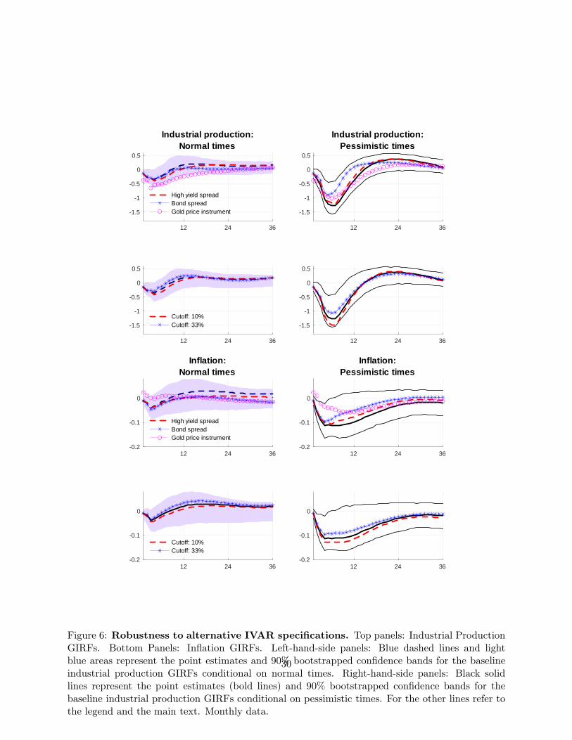
Figure 6: Robustness to alternative IVAR specifications. Top panels: Industrial ProductionGIRFs. Bottom Panels: Inflation GIRFs. Left-hand-side panels: Blue dashed lines and lightblue areas represent the point estimates and 90% bootstrapped confidence bands for the baselineindustrial production GIRFs conditional on normal times. Right-hand-side panels: Black solidlines represent the point estimates (bold lines) and 90% bootstrapped confidence bands for thebaseline industrial production GIRFs conditional on pessimistic times. For the other lines refer tothe legend and the main text. Monthly data.
30
12 24 36
0
20
40
UncertaintyCOVIDinduced unc. shock: Past persist.COVIDinduced unc. shock: Higher persist.COVIDinduced unc. shock: Past pers. & new Fall wave
12 24 36
15
10
5
0
5Industrial production
12 24 362
1
0Inflation
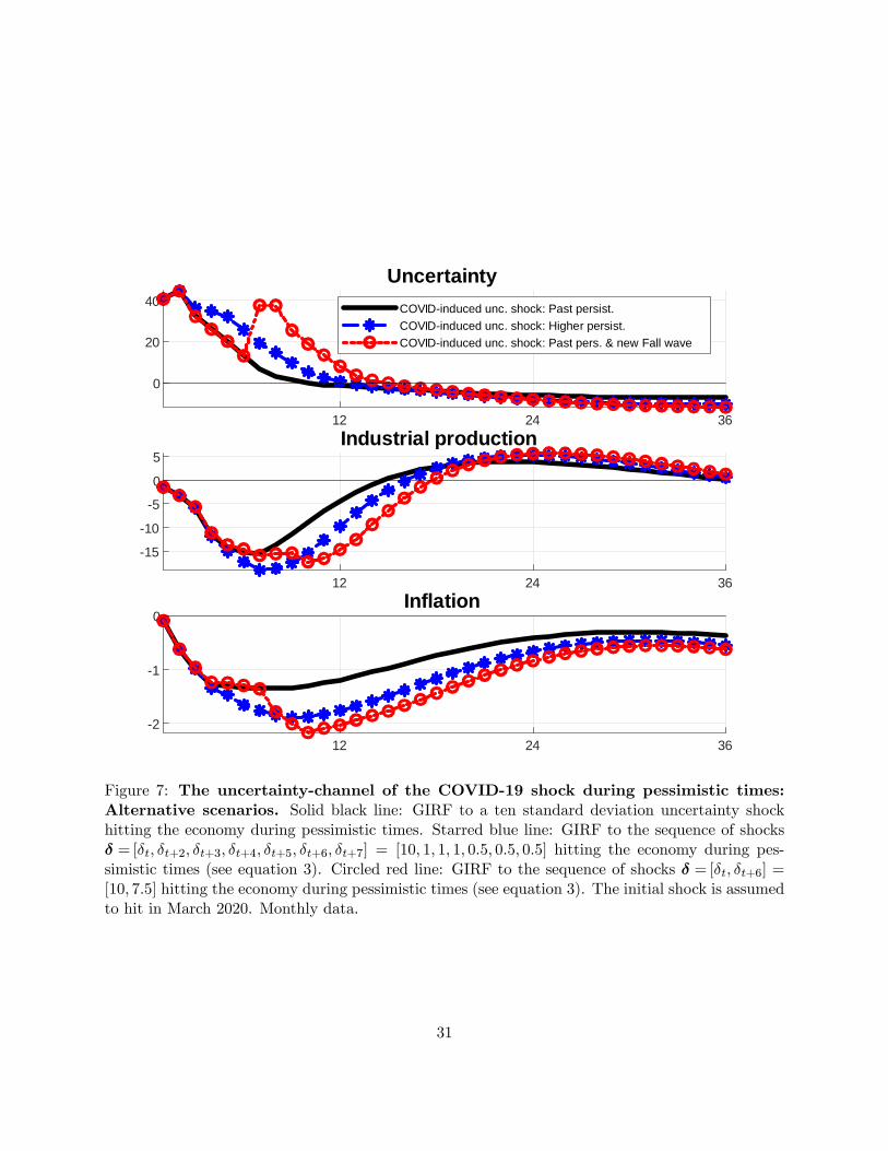
Figure 7: The uncertainty-channel of the COVID-19 shock during pessimistic times:Alternative scenarios. Solid black line: GIRF to a ten standard deviation uncertainty shockhitting the economy during pessimistic times. Starred blue line: GIRF to the sequence of shocksδ = [δt, δt+2, δt+3, δt+4, δt+5, δt+6, δt+7] = [10, 1, 1, 1, 0.5, 0.5, 0.5] hitting the economy during pes-simistic times (see equation 3). Circled red line: GIRF to the sequence of shocks δ = [δt, δt+6] =[10, 7.5] hitting the economy during pessimistic times (see equation 3). The initial shock is assumedto hit in March 2020. Monthly data.
31
Online Appendix"The Impact of Pessimistic Expectations on the Effects of COVID-19-
Induced Uncertainty in the euro Area" by Giovanni Pellegrino, FedericoRavenna and Gabriel Züllig
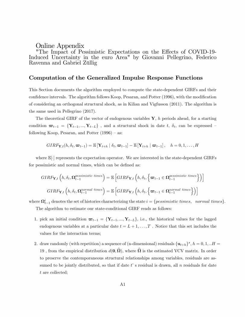
Computation of the Generalized Impulse Response Functions
This Section documents the algorithm employed to compute the state-dependent GIRFs and their
confidence intervals. The algorithm follows Koop, Pesaran, and Potter (1996), with the modification
of considering an orthogonal structural shock, as in Kilian and Vigfusson (2011). The algorithm is
the same used in Pellegrino (2017).
The theoretical GIRF of the vector of endogenous variables Y, h periods ahead, for a starting
condition $t−1 = Yt−1, ...,Yt−L , and a structural shock in date t, δt, can be expressed —following Koop, Pesaran, and Potter (1996) —as:
GIRFY,t(h, δt,$t−1) = E [Yt+h | δt,$t−1]− E [Yt+h |$t−1] , h = 0, 1, . . . ,H
where E[·] represents the expectation operator. We are interested in the state-dependent GIRFsfor pessimistic and normal times, which can be defined as:
GIRFY,t
(h, δt,Ω
pessimistic timest−1
)= E
[GIRFY,t
(h, δt,
$t−1 ∈ Ωpessimistic times
t−1
)]GIRFY,t
(h, δt,Ω
normal timest−1
)= E
[GIRFY,t
(h, δt,
$t−1 ∈ Ωnormal times
t−1
)]whereΩi
t−1 denotes the set of histories characterizing the state i = pessimistic times, normal times.The algorithm to estimate our state-conditional GIRF reads as follows:
1. pick an initial condition $t−1 = Yt−1, ...,Yt−L, i.e., the historical values for the laggedendogenous variables at a particular date t = L+ 1, . . . , T . Notice that this set includes the
values for the interaction terms;
2. draw randomly (with repetition) a sequence of (n-dimensional) residuals ut+hs, h = 0, 1, ..H =
19 , from the empirical distribution d(0, Ω), where Ω is the estimated VCV matrix. In order
to preserve the contemporaneous structural relationships among variables, residuals are as-
sumed to be jointly distributed, so that if date t’s residual is drawn, all n residuals for date
t are collected;
A1
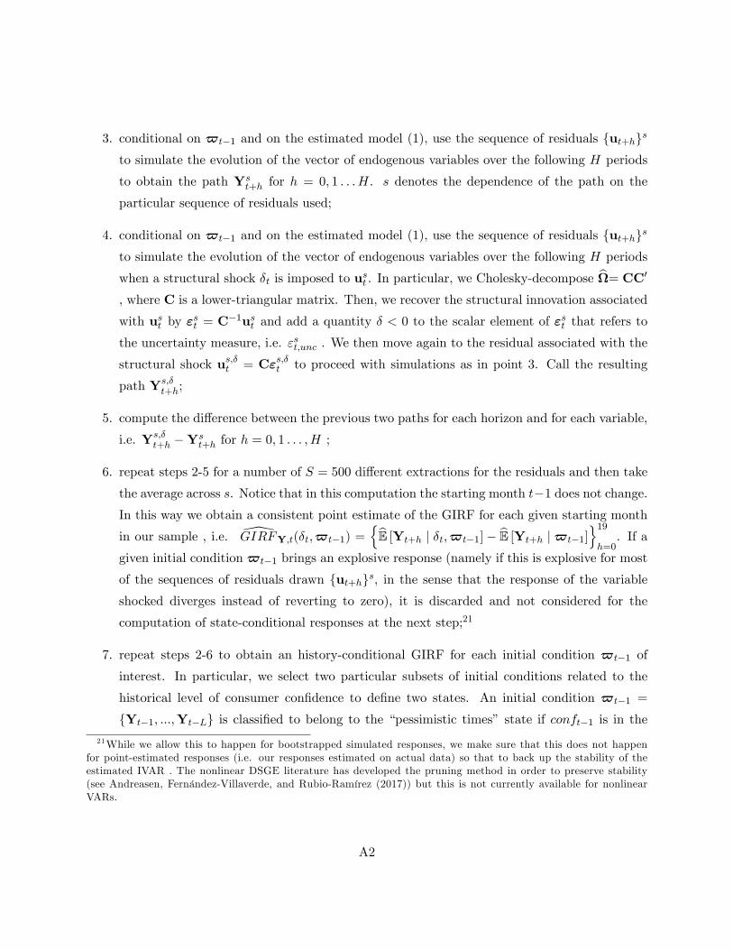
3. conditional on $t−1 and on the estimated model (1), use the sequence of residuals ut+hs
to simulate the evolution of the vector of endogenous variables over the following H periods
to obtain the path Yst+h for h = 0, 1 . . . H. s denotes the dependence of the path on the
particular sequence of residuals used;
4. conditional on $t−1 and on the estimated model (1), use the sequence of residuals ut+hs
to simulate the evolution of the vector of endogenous variables over the following H periods
when a structural shock δt is imposed to ust . In particular, we Cholesky-decompose Ω= CC′
, where C is a lower-triangular matrix. Then, we recover the structural innovation associated
with ust by εst = C−1ust and add a quantity δ < 0 to the scalar element of εst that refers to
the uncertainty measure, i.e. εst,unc . We then move again to the residual associated with the
structural shock us,δt = Cεs,δt to proceed with simulations as in point 3. Call the resulting
path Ys,δt+h;
5. compute the difference between the previous two paths for each horizon and for each variable,
i.e. Ys,δt+h −Ys
t+h for h = 0, 1 . . . , H ;
6. repeat steps 2-5 for a number of S = 500 different extractions for the residuals and then take
the average across s. Notice that in this computation the starting month t−1 does not change.
In this way we obtain a consistent point estimate of the GIRF for each given starting month
in our sample , i.e. GIRFY,t(δt,$t−1) =E [Yt+h | δt,$t−1]− E [Yt+h |$t−1]
19
h=0. If a
given initial condition $t−1 brings an explosive response (namely if this is explosive for most
of the sequences of residuals drawn ut+hs, in the sense that the response of the variableshocked diverges instead of reverting to zero), it is discarded and not considered for the
computation of state-conditional responses at the next step;21
7. repeat steps 2-6 to obtain an history-conditional GIRF for each initial condition $t−1 of
interest. In particular, we select two particular subsets of initial conditions related to the
historical level of consumer confidence to define two states. An initial condition $t−1 =
Yt−1, ...,Yt−L is classified to belong to the “pessimistic times” state if conft−1 is in the
21While we allow this to happen for bootstrapped simulated responses, we make sure that this does not happenfor point-estimated responses (i.e. our responses estimated on actual data) so that to back up the stability of theestimated IVAR . The nonlinear DSGE literature has developed the pruning method in order to preserve stability(see Andreasen, Fernández-Villaverde, and Rubio-Ramírez (2017)) but this is not currently available for nonlinearVARs.
A2
bottom 20% of the consumer confidence empirical distribution and to the “normal times”
state if conft−1 is in not in its bottom 20%;
8. history-dependent GIRFs obtained in step 7 are then averaged over the state they belong to
produce our estimate of the state-dependent GIRFs, i.e., our
GIRFY,t
(δt,Ω
pessimistic timest−1
)and GIRFY,t
(δt,Ω
normal timest−1
);
9. confidence bands around the point estimates obtained in point 8 are computed through boot-
strap22. In particular, we simulate R = 500 datasets statistically equivalent to the actual
sample and for each of them interaction terms are constructed coherently with the simulated
series. Then, for each dataset, (i) we estimate our Interacted VAR model and (ii) implement
steps 1-8. In implementing the procedure the starting conditions and the VCV matrix used in
the computation depend on the particular dataset r used, i.e. $rt−1 and Ωr. Of the resulting
distribution of state-conditional GIRFs, we take the 5th and 95th percentiles to construct the
90% confidence bands.
Computation of the Generalized Forecast Error Variance Decom-
position
The algorithm for the computation of the state-dependent Generalized Forecast Error Variance De-
composition (GFEVD) for our nonlinear VAR model follows Caggiano, Castelnuovo, and Pellegrino
(2017). In particular, the innovations to the algorithm proposed in Lanne and Nyberg (2016) are:
i) it is designed to simulate the importance of an orthogonal structural shock, and ii) it considers
a one standard deviation shock in each variable. The expression at the basis of our computation
of the GFEVD is the same proposed by Lanne and Nyberg (2016, equation 9).
In particular, conditional on a specific initial history $t−1 and a forecast horizon of interest z,
the GFEVDij that refers to a variable i and a shock j whose size is δjt is given by:
GFEVDij(z,$t−1) =
∑zh=0GIRFYi(h, δ
jt ,$t−1)2∑n
j=1
∑zh=0GIRFYi(h, δ
jt ,$t−1)2
i, j = 1, ..., n, (A1)
where h is an indicator keeping track of the forecast ahead, and n denotes the number of variables
22The bootstrap used is similar to the one used by Christiano, Eichenbaum and Evans (1999, footnote 23). Ourcode repeats the explosive artificial draws to be sure that exactly 500 draws are used.
A3
in the vector Y.23 Differently from Lanne and Nyberg (2016), in our case the object GIRFYi(·) inthe formula refers to GIRFs à la Koop, Pesaran, and Potter (1996) computed by considering an
orthogonal shock as in Kilian and Vigfusson (2011).24 In our application we are interested in the
contribution of an identified uncertainty shock to the GFEVD of all the variables in the vector Y.
Further, while formula (A1) defines the GFEVD for a given history, we are interested in computing
a state-conditional GFEVD referring to a set of histories.
Given our model (1), we compute our state-dependent GFEVD for normal times and pessimistic
times by following the steps indicated below. In particular, we:
1. consider an orthogonal shock equal to a standard deviation in each variable of the estimated
I-VAR model. This is equivalent, for a Cholesky decomposition, to taking a vector of shocks
equal to(δ1t , δ
2t , ..., δ
nt
)= (1, 1, ..., 1) in our algorithm in the previous Section;25
2. pick a history $t−1 from the set of all histories;
3. compute the GIRFY(·, ·,$t−1) for each δjt (j = 1, ..., n) and for each h ≤ z according to
points 2-6 of the algorithm in the previous Section;
4. plug the GIRFs computed in step 3 into equation (A1) to obtain GFEV Dij(z,$t−1) for the
particular forecast horizon z and history $t−1 considered;
5. repeat steps 2—4 for all the histories, distinguishing between the histories belonging to the
"normal times" state and the "pessimistic times" state (see the definition in point 7 of the
GIRFs algorithm);
6. compute the state-dependent GFEVD for the "normal times" state and the "pessimistic
times" state by computing the average of the GFEVDij(z,$t−1) across all the histories
relevant for the two states.23Expression (A1) gives a GFEVD that by construction lies between 0 and 1, and for which the contribution of all
the shocks on a given variable sum to 1.24The object GIRFYi(·) in Lanne and Nyberg’s (2016) expression refers to the GIRFs à la Pesaran and Shin (1998).
This definition of the GIRF refers to a non-orthogonalized shock and it can be applied both to linear and to nonlinearVAR models. Details can be found in Pesaran and Shin (1998) and Lanne and Nyberg (2016).25The size of the shock matters in a nonlinear model. The use of a one standard deviation shock in all variables allows
our GFEVD algorithm to return the usual Forecast Error Variance (FEV) and Forecast Error Variance Decomposition(FEVD) quantities referred to an orthogonal shock when the algorithm is applied to a standard linear VAR model.
A4

Proxy Structural Interacted VAR models
Our reduced-form Interacted VAR model can be written as:
Yt = α+
L∑j=1
AjYt−j +
L∑j=1
cjunct−j · conft−j
+ ut,
from where the corresponding Structural IVAR model can be obtained as:
Yt = α+L∑j=1
AjYt−j +
L∑j=1
cjunct−j · conft−j
+ B−10 νt,
where Yt is a vector of variables of interest, Aj and cj , j = 1, ..., L , are coeffi cient matrices and
coeffi cient vectors, respectively, and νt is a vector of economically meaningful structural shocks
that are a linear combination of the reduced-form IVAR residuals, i.e., εt = B−10 νt. Suppose we
are interested in partial identification and, in particular, in the impulse response of a shock νit ∈ νt.This means that we only need to identify the i-th column of the matrix B−1
0 , b−10,i . Call the other
columns as B−10,ı . Consequently, we can rewrite εt = B−1
0 νt as:
εt = b−10,i νit + B−1
0,ı ν ıt
A Proxy Structural IVAR model allows us to identify the impact vector b−10,i by means of an
instrument mt that satisfies the following conditions:
E [mtνit] = φ 6= 0 (Relevance condition)
E [mtν ıt] = 0 (Exogeneity condition).
The previous conditions imply:
E [mtεt] = b−10,iφ,
or: E [mtε1t]
E [mtε2t]
.
E [mtεNt]
=
b−1
0,i (1)φ
b−10,i (2)φ
.
b−10,i (N)φ
,
A5

where b−10,i (z), z = 1, ..., N , denotes z-th element of the vector b−1
0,i . Without loss of generality,
assume that we are interested in the effects of the first shock, or i = 1. Hence with E [mtεt] in hand
we can recover the normalized impact vector as:
1
E[mtε2t]E[mtε1t]
.E[mtεNt]E[mtε1t]
=
1
b−10,1(2)
b−10,1(1)
.b−1
0,1(N)
b−10,1(1)
,
which corresponds to the impact vector for an unitary shock,[1; b−1
0,1(1)/b−10,1(1)
]. An estimate of
b−10,1(1)/b−1
0,1(1) can be obtained from the two stage least square regression of ε1t on ε1t using the
instrument mt. The first stage regression:
ε1t = βmt + ξt
yields the fitted values ε1t, which are then used in the second stage regression to recover the true
normalized impact vector:
ε1t = γεit + ςt.
=b−1
0,1(1)
b−10,1(1)
εit + ςt,
where the recoverability of b−10,1(1)/b−1
0,1(1) depends on the fact that E [mtεt] = b−10,1φ.
26
The (absolute) impact vector b−10,1 can then be derived from the estimated reduced form variance-
covariance matrix, Σ = E [εtε′t], as explained, e.g., in Gertler and Karadi (2015).
27 At this point
we can compute the impulse response function to a one standard deviation shock in date t, δt = 1,
26 Indeed, we have: γ =E[ε1tεit]E[ε2it]
=E[ε1tβmt]E[β2m2
t ]=
βE[ε1tmt]β2E[m2
t ]=
E[ε1tmt]
E[m2t ]
E[ε1tmt](E[ε1tmt]
E[m2t ]
)2
·E[m2t ]=
E[ε1tmt]E[ε1tmt]
=φb−1
0,1(1)
φb−10,1(1)
.
27Specifically, to recover the absoulte impact vector we follow Piffer’s notes on the identification of VARs usingexternal instruments available at https://sites.google.com/site/michelepiffereconomics/ .
A6
to ν1t, according to the usual Generalized IRF à la Koop, Pesaran, and Potter (1996):
GIRFY,t(h, 1,$t−1) = E [Yt+h | δt = 1,$t−1]− E [Yt+h |$t−1] , for h = 0, 1, ...,H
=
b−1
0,1 , for h = 0
E[Yt+h |δt = 1,$t−1] − E[Yt+h |$t−1] , for h = 1, ...,H,
where $t−1 denotes the initial condition, or Yt−1, ...,Yt−L. In computing the GIRF we followthe same algorithm outlined earlier.
Supplementary results
Figure A1 plots the time series that enter our baseline IVAR.
Figure A2 plots the daily VSTOXX index, our proxy for euro area financial uncertainty, against
its monthly average.
Figure A3 in its upper panel plots the consumer confidence indicator released by the european
Commission in April —a leading indicator of future economic activity —, which signaled a confidence
level approaching the number reached during the 2008-2009 financial crisis. The bottom panel of
Figure A3 plots the monthly VSTOXX, our baseline measure of financial uncertainty, which in
March 2020 reached levels comparable to the global financial crisis.
Figure A4 plots all the uncertainty indicators we use in our analysis, as described in the robust-
ness checks Section of the paper.
Figure A5 plots all the indices of survey-based confidence we use in our analysis, as described
in the robustness checks Section of the paper.
Figure A6 plots the pessimistic-times state under the alternative interpretation of pessimism
based on "mood swings", i.e., sudden negative changes in the consumer confidence series. We
classify an initial month to the pessimistic-times state whenever the cumulative change in the last
six months of the Consumer Confidence Index is in its bottom 20%.28 In this way, pessimistic times
only include phases of negative mood swings.
Figure A7 and Table A1 complement the findings in Figure 7 and Table 2 of the paper. They
show that, in a situation in which consumer confidence is not allowed to mean revert for the first
6 months after the shock, the same shocks considered in Section 3.2 imply larger peak losses and
28This threshold corresponds to a cumulative change of −2.5.
A7
more time to rebound in the case of a new fall wave.29 This means that in our findings in Section
3.2 we are conservative about the possible losses implied by the COVID-19-induced uncertainty
shock.
29We compute the GIRF for a counterfactual where the consumer confidence level (for each of the shocked pathsbehind the average shocked path in equation 2 of the main paper, E [Yt+h | δt,$t−1]) is not allowed to increase ifnot after 6 months. If the consumer confidence would increase, a counterfactual shock keeps its level constant to thelast value.
A8
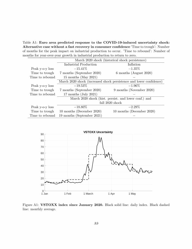
Table A1: Euro area predicted response to the COVID-19-induced uncertainty shock:Alternative case without a fast recovery in consumer confidence ’Time to trough’: Numberof months for the peak impact on industrial production to occur. ’Time to rebound’: Number ofmonths for year-over-year growth in industrial production to return to zero.
March 2020 shock (historical shock persistence)Industrial Production Inflation
Peak y-o-y loss −15.41% −1.35%Time to trough 7 months (September 2020) 6 months (August 2020)Time to rebound 15 months (May 2021) −
March 2020 shock (increased shock persistence and lower confidence)Peak y-o-y loss −19.53% −1.96%Time to trough 7 months (September 2020) 9 months (November 2020)Time to rebound 17 months (July 2021) −
March 2020 shock (hist. persist. and lower conf.) andfall 2020 shock
Peak y-o-y loss −18.80% −2.29%Time to trough 10 months (December 2020) 10 months (December 2020)Time to rebound 19 months (September 2021) −
1 Jan 1 Feb 1 March 1 Apr 1 May0
10
20
30
40
50
60
70
80
90VSTOXX Uncertainty
Figure A1: VSTOXX index since January 2020. Black solid line: daily index. Black dashedline: monthly average.
A9
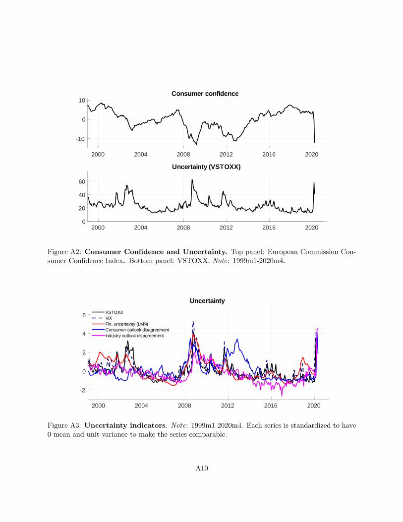
2000 2004 2008 2012 2016 2020
10
0
10Consumer confidence
2000 2004 2008 2012 2016 20200
20
40
60
Uncertainty (VSTOXX)
Figure A2: Consumer Confidence and Uncertainty. Top panel: European Commission Con-sumer Confidence Index. Bottom panel: VSTOXX. Note: 1999m1-2020m4.
2000 2004 2008 2012 2016 2020
2
0
2
4
6
UncertaintyVSTOXXVIXFin. uncertainty (LMN)Consumer outlook disagreementIndustry outlook disagreement
Figure A3: Uncertainty indicators. Note: 1999m1-2020m4. Each series is standardized to have0 mean and unit variance to make the series comparable.
A10
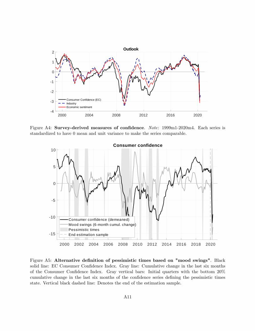
2000 2004 2008 2012 2016 20204
3
2
1
0
1
2Outlook
Consumer Confidence (EC)IndustryEconomic sentiment
Figure A4: Survey-derived measures of confidence. Note: 1999m1-2020m4. Each series isstandardized to have 0 mean and unit variance to make the series comparable.
Consumer confidence
2000 2002 2004 2006 2008 2010 2012 2014 2016 2018 2020
15
10
5
0
5
10
Consumer confidence (demeaned)Mood swings (6month cumul. change)Pessimistic timesEnd estimation sample
Figure A5: Alternative definition of pessimistic times based on "mood swings". Blacksolid line: EC Consumer Confidence Index. Gray line: Cumulative change in the last six monthsof the Consumer Confidence Index. Gray vertical bars: Initial quarters with the bottom 20%cumulative change in the last six months of the confidence series defining the pessimistic timesstate. Vertical black dashed line: Denotes the end of the estimation sample.
A11

12 24 36
0
20
40
UncertaintyCOVIDinduced unc. shock: Past persist.COVIDinduced unc. shock: Higher pers. & low conf.COVIDinduced unc. shock: Past pers., low conf. & Fall wave
12 24 36
1510
505
Industrial production
12 24 36
2
1
0Inflation
Figure A6: The uncertainty-channel of the COVID-19 shock during pessimistic times:Alternative scenarios (case without a fast recovery in consumer confidence). Solid blackline: GIRF to a ten standard deviation uncertainty shock hitting the economy during pessimistictimes. Starred blue line: GIRF to the sequence of shocks δ = [δt, δt+2, δt+3, δt+4, δt+5, δt+6, δt+7] =[10, 1, 1, 1, 0.5, 0.5, 0.5] hitting the economy during pessimistic times (see equation 3 in the mainpaper). Circled red line: GIRF to the sequence of shocks δ = [δt, δt+6] = [10, 7.5] hitting theeconomy during pessimistic times (see equation 3). Note: x -axis in months. The initial shock isassumed to hit in March 2020. The subsequent shocks are the same considered for the exercise inFigure 7 in the main paper. For the computation of the counterfactual GIRF please see foonote29.
A12

WO RK ING PAPE R — DA N MARK S NA T IO NA LB ANK
X X M O N T H 2 0 2 0 — N O . X X
As a rule, Working Papers are not translated, but are available in the original language used by the contributors. Danmarks Nationalbank’s Working Papers are published in PDF format at www.nationalbanken.dk. A free electronic subscription is also available at the website. The subscriber receives an email notification whenever a new Working Paper is published. Text may be copied from this publication provided that the source is specifically stated. Changes to or misrepresentation of the content is not permitted. Please direct any enquiries directly to the contributors or to Danmarks Nationalbank, Communications, [email protected].