Effects of Inflation and Wage Expectations on Consumer Spending: Evidence from Micro Data Yuichiro Ito* yuuichirou.itou@boj.or.jp Sohei Kaihatsu* souhei.kaihatsu@boj.or.jp

No.16-E-7 June 2016

Bank of Japan 2-1-1 Nihonbashi-Hongokucho, Chuo-ku, Tokyo 103-0021, Japan

* Monetary Affairs Department

Papers in the Bank of Japan Working Paper Series are circulated in order to stimulate discussion and comments. Views expressed are those of authors and do not necessarily reflect those of the Bank. If you have any comment or question on the working paper series, please contact each author.

When making a copy or reproduction of the content for commercial purposes, please contact the Public Relations Department (post.prd8@boj.or.jp) at the Bank in advance to request permission. When making a copy or reproduction, the source, Bank of Japan Working Paper Series, should explicitly be credited.

Bank of Japan Working Paper Series

1

Effects of Inflation and Wage Expectations on Consumer Spending: Evidence from Micro Data*

Yuichiro Ito† and Sohei Kaihatsu‡

June, 2016

Abstract

This paper employs a unique micro dataset in Japan to monitor inflation and wage expectations and investigate their effects on consumer spending. Based on our analysis, wage expectations increased moderately among wider range of employees after the introduction of Quantitative and Qualitative Monetary Easing (QQE). Real wage expectations also recovered recently, although it declined soon after the introduction of QQE, reflecting larger increases in inflation expectations compared with wage expectations. Increases in inflation expectations produced the positive effect on consumer spending on the whole since the positive effect of declines in real interest rates was larger than the negative effect of declines in real wage expectations. Wage expectations were generally influenced by wage perception and business performance outlook. This suggests that improvement in wage expectations needs to associate higher expectations about business performance outlook and realization of wage increases.

JEL classification: D12, D84, D91, E21, E52

Keywords: inflation expectations, wage expectations, Carlson–Parkin method, survey data,

Quantitative and Qualitative Monetary Easing.

* We would like to thank the staff of the Bank of Japan for their helpful comments. The data for this

analysis, “The Questionnaire Survey on Work and Life of Workers (conducted by Japanese Trade

Union Confederation Research Institute for Advancement of Living Standards),” was provided by

the Social Science Japan Data Archive, Center for Social Research and Data Archives, Institute of

Social Science, The University of Tokyo, and Japanese Trade Union Confederation Research

Institute for Advancement of Living Standards. The views expressed here, as well as any remaining

errors, are those of the authors and should not be ascribed to the Bank of Japan or the Monetary

Affairs Department.

† Monetary Affairs Department, Bank of Japan (E-mail: yuuichirou.itou@boj.or.jp) ‡ Monetary Affairs Department, Bank of Japan (E-mail: souhei.kaihatsu@boj.or.jp) 

2

1. Introduction

Households make economic decisions on the basis of the outlook for inflation and

wages as well as current economic conditions. Therefore, monitoring expectations

regarding both inflation and wages is important for considering the effects of monetary

policy on consumer spending as these reflect households’ future outlook for the

economy. Thus far, much effort has been devoted to characterizing the behavior of

inflation expectations, using survey data.1 However, only a few previous studies exist

regarding empirical analyses on wage expectations partly due to data constraints.

Most researches among the available literature focus on the impact of inflation

expectations on consumer spending. Ichiue and Nishiguchi (2015) find evidence to

support the prediction that rising inflation expectations boost current spending at the

zero lower bound on nominal interest rates; this relation appears to be stronger for asset

holders and older people according to Japanese micro data from the “Opinion Survey on

the General Public’s Views and Behavior” conducted by the Bank of Japan. In Europe,

D’Acunto et al. (2015) document a positive cross-sectional association between

households’ inflation expectations and their willingness to purchase durable

consumption goods by exploiting the German natural experiment of an increase in value

added tax. On the other hand, both Burke and Ozdagli (2013) and Bachmann et al.

(2015) perform empirical analyses using US micro data. They report contradictory

results about the effect of rising inflation expectations on current consumption of

durable goods. Thus, no consensus has been reached regarding the relation between

inflation expectations and consumer spending.

In this regard, Burke and Ozdagli (2013) report that households in their sample, on

average, did not expect wage growth to match inflation; therefore, an increase in

expected inflation would create a negative income effect that discouraged spending in

both the present and future. This result indicates that when analyzing households’

decisions about consumer spending, investigating the effect of wage expectations as

well as the effect of inflation expectations is important. The effects of rising inflation

expectations on consumer spending may vary depending on whether those expectations

reflect an increase in commodity prices or a change in expectations caused by the

monetary policy. Moreover, clarifying the impact of the relative relation between

inflation and wage expectations on the real economy is important for assessing whether 1 See Nishiguchi et al. (2014) and Kamada et al. (2015) for recent studies on households’ inflation

expectations in Japan.

3

rising inflation expectations lead to a virtuous cycle from income to spending.

The importance of measuring wage expectations has been broadly recognized.

Bernanke (2007) remarks that measuring wage expectations provides useful information

for monitoring households’ inflation expectations although he indicates that data on

wage expectations is particularly scarce.2 Bruine de Bruin et al. (2010) indicate that

wage expectations affect consumers’ decisions across different periods and are thus of

great value for understanding and forecasting economic behaviors. Moreover, Potter

(2011) remarks that discrepancies between expected wage changes and expected

inflation may affect household financial decisions. He emphasizes the importance of

monitoring the relative relation between inflation and wage expectations.

This paper aims to investigate the effect of households’ inflation expectations on their

consumer spending, considering changes in wage expectations. It uses Japanese micro

data from the “Questionnaire Survey on Work and Life of Workers” (hereafter the

Workers Survey) conducted by Japanese Trade Union Confederation (RENGO)

Research Institute for Advancement of Living Standards (hereafter RENGO-RIALS).

There are three important contributions from our analysis.

First, this paper focuses on households’ wage expectations, which have not yet been

analyzed sufficiently due to data limitations, by employing unique micro data in Japan.

We investigate the development of wage expectations and the relative relation between

inflation and wage expectations after the introduction of quantitative and qualitative

monetary easing (hereafter QQE) by the Bank of Japan. To the best of our knowledge, the

Workers Survey is the only survey to have systematically collected data on households’

forecasts for price, wage, and consumption for a long time period in Japan.

Second, this paper analyzes the effects of inflation expectations on the real economy

through households’ consumer spending, considering changes in wage expectations. The

effects of rising inflation expectations on households’ behaviors are likely to differ

between the period of rising inflation expectations against the background of the

commodity price surge in 2007–08 and the period after the introduction of QQE in 2013.

This seems attributable to differences in households’ sentiments, such as the outlook for

economic conditions and business performance between these two periods. In this paper,

we examine the conditions under which expectations of rising inflation stimulates

2 Recognizing this problem, many countries have sought to start a new survey project. See Van der

Klaauw et al. (2008) for details on the survey project in the US.

4

current consumer spending.

Third, this paper investigates how wage expectations are formed. We analyze the

relation between wage expectations and responses given to other questions in the

Workers Survey to examine the conditions under which wage expectations continue to

rise steadily.

The remainder of this paper is organized as follows. Section 2 provides an overview

of the survey data through a comparison with other household inquiries in Japan.

Section 3 describes the modified Carlson–Parkin method in a pentachotomous case,3,4

which is used as a quantification method of qualitative survey data. It investigates

developments of inflation and wage expectations and their relative relation. Section 4

analyzes the effect of inflation expectations on consumer spending, considering changes

in wage expectations. Section 5 investigates how wage expectations are formed. Section

6 presents the conclusion. The Appendix provides details of the modified Carlson–

Parkin method in this paper.

2. Overview of survey data

In this paper, we construct a novel dataset combining household wage and inflation

expectations together with the data on consumer spending based on the micro data from

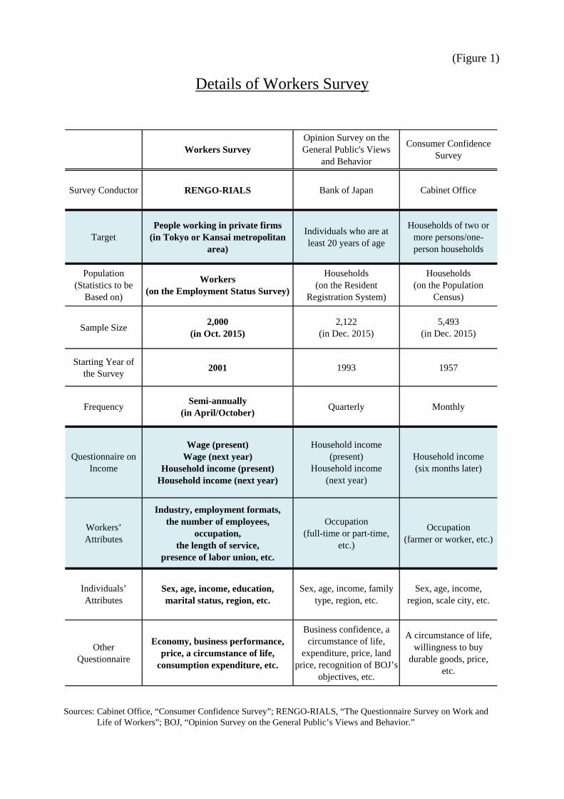
the Workers Survey conducted by RENGO-RIALS. Figure 1 illustrates an overview of

the Workers Survey and compares it with other well-known household surveys, such as

the “Opinion Survey on the General Public’s Views and Behavior” (conducted by the

Bank of Japan) and the “Consumer Confidence Survey” (conducted by the Cabinet

Office). The Workers Survey started in April 2001 and has been conducted

semiannually to investigate workers’ outlook for economic and labor conditions. Until

April 2010, responses had been obtained via the mail survey method, and since the 20th

survey in October 2010, responses have been obtained via the Internet-monitor survey

method. Since the introduction of the Internet-monitor survey method, the survey’s

sample size has been 2,000 respondents, which is comparable to the other well-known

household surveys.

The Workers Survey is conducted for individuals who work at private firms in the

3 The term pentachotomous originates from the Greek word meaning “fivefold.” 4 We extend the standard Carlson–Parkin method to deal with a questionnaire with five choices and

modify it to adjust the survey data to deal with some distortions, as explained later.

5

Tokyo or Kansai metropolitan areas.5 The survey differs from the “Opinion Survey on

the General Public’s Views and Behavior” and “Consumer Confidence Survey,” both of

which are conducted at the household level and include the retired and the unemployed.

In addition, it is characteristic that the Workers Survey collects data on wage income,

whereas the other household surveys investigate total household income. Here, careful

attention should be paid to the point that total income includes pensions, asset income,

and spousal income as well as wages. Moreover, the survey investigates a wide range of

topics, such as perceptions and outlook toward price and consumption, which are likely

to have a strong connection with wage expectations. Therefore, for example, it is

possible to analyze the effect of inflation expectations on households’ consumer

spending based on the same set of samples. To the best of our knowledge, the Workers

Survey is the only survey in Japan to systematically collect data on households’ outlook

regarding price, wages, and consumption for a long time period.6

It is also characteristic that the Workers Survey contains much information about

respondents’ attributes regarding the firms in which they are employed and their

employment formats. For example, the survey collects data on the number of employees

in the employing firm, industry, presence of labor union, type of employment, and

employment longevity. Therefore, it is possible to analyze the data by controlling for the

effects of various attributes.7 While we mainly analyze the outlook for price, wage,

economic conditions, business performance, and consumption across the whole sample,

we also perform our sub-sample analysis based on attributes, such as the number of

employees in the employing firm, industry, and type of employment.

The survey inquires about price and wage changes from the previous year in

questions. For example, the survey question about forecasts for price asks, “What is

your outlook for price one year from now?” and the respondents are required to select

from six choices: “will go up significantly,” “will go up slightly,” “will remain almost

unchanged,” “will go down slightly,” “will go down significantly,” and “unknown.” In

this paper, we remove the respondents who select “unknown” and analyze the data

based on the respondents who selected the other five choices. Furthermore, the survey

5 In the survey, respondents are randomly selected from registered private workers based on the

Employment Status Survey. 6 As a study based on the Workers Survey, Oguma and Nagumo (2011) investigate a development of anxiety about unemployment and the effect of the presence of a labor union on easing uncertainty about life. 7 For details of respondents’ attributes in the survey, see the reference figure.

6

investigates forecasts covering three years from now in the questions of price, economic

conditions, and business performance. In addition, it investigates forecasts for three and

five years from now in the question on wages in April since 2013. Therefore, we

analyze not only short-term expectations covering one year from now but also

long-term expectations for three and five years from now.

3. Measuring wage expectations

This section introduces methodology to estimate wage expectations. We then

investigate the development of wage expectations in Japan amid expectations of rising

inflation after the introduction of QQE by the Bank of Japan. For details of the

estimation method, see the attached Appendix.

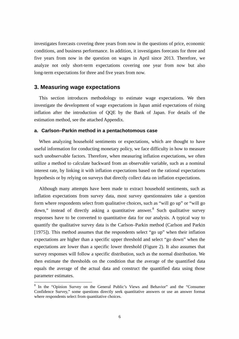
a. Carlson–Parkin method in a pentachotomous case

When analyzing household sentiments or expectations, which are thought to have

useful information for conducting monetary policy, we face difficulty in how to measure

such unobservable factors. Therefore, when measuring inflation expectations, we often

utilize a method to calculate backward from an observable variable, such as a nominal

interest rate, by linking it with inflation expectations based on the rational expectations

hypothesis or by relying on surveys that directly collect data on inflation expectations.

Although many attempts have been made to extract household sentiments, such as

inflation expectations from survey data, most survey questionnaires take a question

form where respondents select from qualitative choices, such as “will go up” or “will go

down,” instead of directly asking a quantitative answer.8 Such qualitative survey

responses have to be converted to quantitative data for our analysis. A typical way to

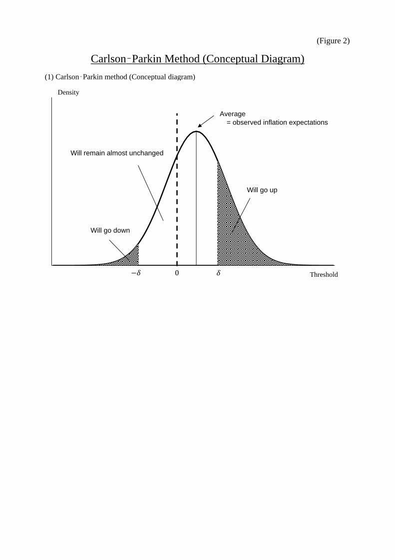
quantify the qualitative survey data is the Carlson–Parkin method (Carlson and Parkin

[1975]). This method assumes that the respondents select “go up” when their inflation

expectations are higher than a specific upper threshold and select “go down” when the

expectations are lower than a specific lower threshold (Figure 2). It also assumes that

survey responses will follow a specific distribution, such as the normal distribution. We

then estimate the thresholds on the condition that the average of the quantified data

equals the average of the actual data and construct the quantified data using those

parameter estimates. 8 In the “Opinion Survey on the General Public’s Views and Behavior” and the “Consumer Confidence Survey,” some questions directly seek quantitative answers or use an answer format where respondents select from quantitative choices.

7

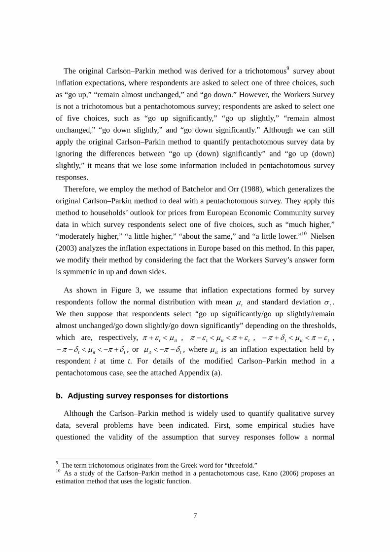
The original Carlson–Parkin method was derived for a trichotomous9 survey about

inflation expectations, where respondents are asked to select one of three choices, such

as “go up,” “remain almost unchanged,” and “go down.” However, the Workers Survey

is not a trichotomous but a pentachotomous survey; respondents are asked to select one

of five choices, such as “go up significantly,” “go up slightly,” “remain almost

unchanged,” “go down slightly,” and “go down significantly.” Although we can still

apply the original Carlson–Parkin method to quantify pentachotomous survey data by

ignoring the differences between “go up (down) significantly” and “go up (down)

slightly,” it means that we lose some information included in pentachotomous survey

responses.

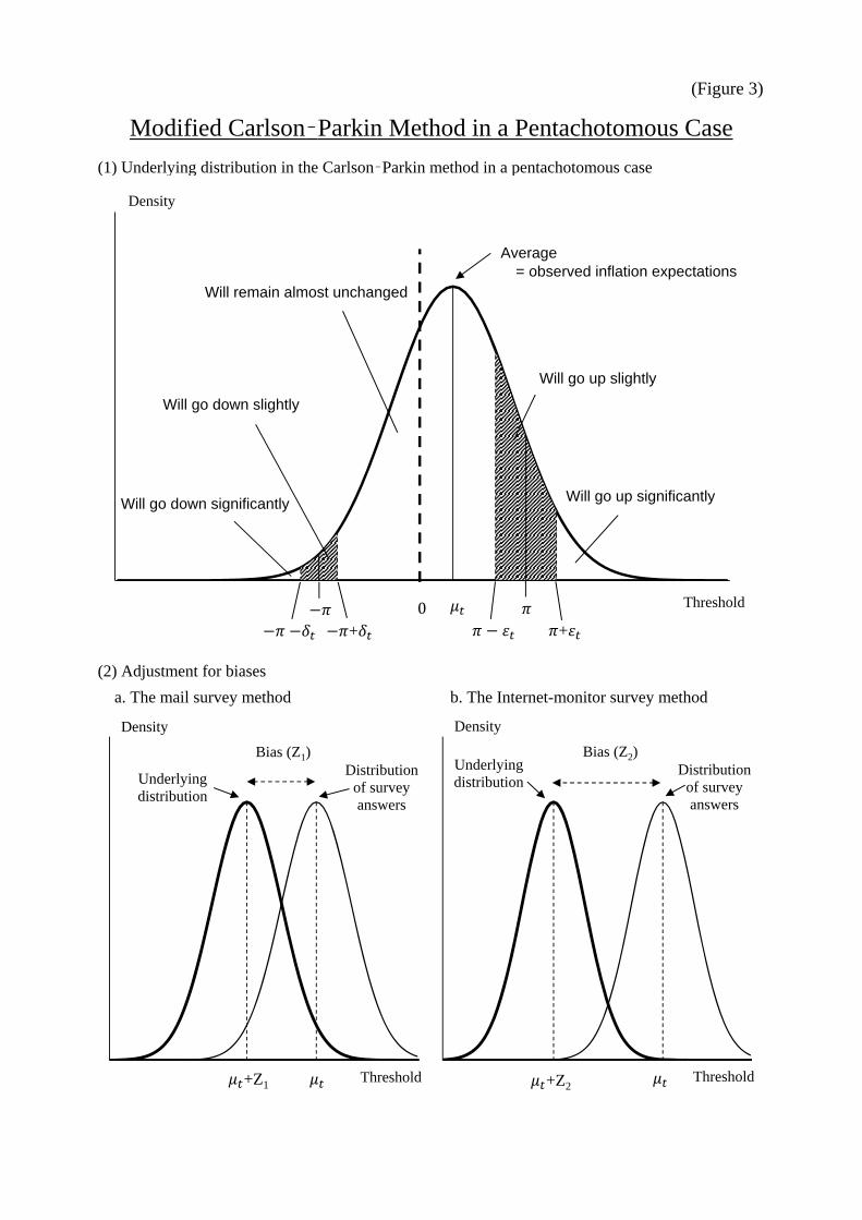
Therefore, we employ the method of Batchelor and Orr (1988), which generalizes the

original Carlson–Parkin method to deal with a pentachotomous survey. They apply this

method to households’ outlook for prices from European Economic Community survey

data in which survey respondents select one of five choices, such as “much higher,”

“moderately higher,” “a little higher,” “about the same,” and “a little lower.”10 Nielsen

(2003) analyzes the inflation expectations in Europe based on this method. In this paper,

we modify their method by considering the fact that the Workers Survey’s answer form

is symmetric in up and down sides.

As shown in Figure 3, we assume that inflation expectations formed by survey

respondents follow the normal distribution with mean t and standard deviation t .

We then suppose that respondents select “go up significantly/go up slightly/remain

almost unchanged/go down slightly/go down significantly” depending on the thresholds,

which are, respectively, itt , titt , titt ,

titt , or tit , where it is an inflation expectation held by

respondent i at time t. For details of the modified Carlson–Parkin method in a

pentachotomous case, see the attached Appendix (a).

b. Adjusting survey responses for distortions

Although the Carlson–Parkin method is widely used to quantify qualitative survey

data, several problems have been indicated. First, some empirical studies have

questioned the validity of the assumption that survey responses follow a normal

9 The term trichotomous originates from the Greek word for “threefold.” 10 As a study of the Carlson–Parkin method in a pentachotomous case, Kano (2006) proposes an estimation method that uses the logistic function.

8

distribution. In this regard, as indicated by Kano (2006), it seems reasonable to assume

the existence of a standard and tractable normal distribution in a situation where there is

little information about distribution of expectations. We thus assume the normal

distribution in this paper, but the estimates should be interpreted with some latitude.

Second, the assumption of constant and symmetric thresholds is also questioned since

it is thought that distortions exist in survey responses. Based on data from the “Opinion

Survey on the General Public’s Views and Behavior,” Kamada (2013) indicates the

following distortions in household responses in Japan: there are too many integers,

zeros, and multiples of five but too few negative values. He also reveals that the

presence of many zeros and of few negative values suggests that many households give

an answer of 0% even if they actually expect deflation, which implies that there exists

downward rigidity in households’ answers on inflation expectations. If any distortions

exist in survey responses, it is impossible to apply the original Carlson–Parkin method,

which assumes the symmetric thresholds.

To deal with these distortions, it is necessary to relax the assumption of constant and

symmetric thresholds as well as the long-term equality between perceived and expected

values. In this regard, many studies propose methods to modify the original Carlson–

Parkin method. Hori and Terai (2005) suggest an approach that allows for time variation

in and asymmetry of thresholds by assuming the rational expectations hypothesis. Kano

(2006) also proposes a method to allow for asymmetry of thresholds by supposing that

the dispersion of survey responses equals that of the actual series. Furthermore, Sekine

et al. (2008) obtain inflation expectations using the ordinary least squares method by

assuming the existence of distortions in survey answers.

In addition to the distortions peculiar to survey responses about inflation expectations,

other types of distortions exist regarding the use of mail survey or Internet-monitor

survey methods. Honda and Honkawa (2005) mention that significant differences exist

in survey responses between surveys using the mail survey and Internet-monitor survey

methods. In particular, they indicate that negative responses, such as anxiety and

complaints, tend to be observed more often in the Internet-monitor survey. These

distortions must be considered to quantify qualitative data using the Carlson–Parkin

method. In fact, the Workers Survey had been conducted via mail survey method until

April 2010 and had been conducted via Internet-monitor survey method since October

2010. Recently, the Internet-monitor survey has become more popular, considering

9

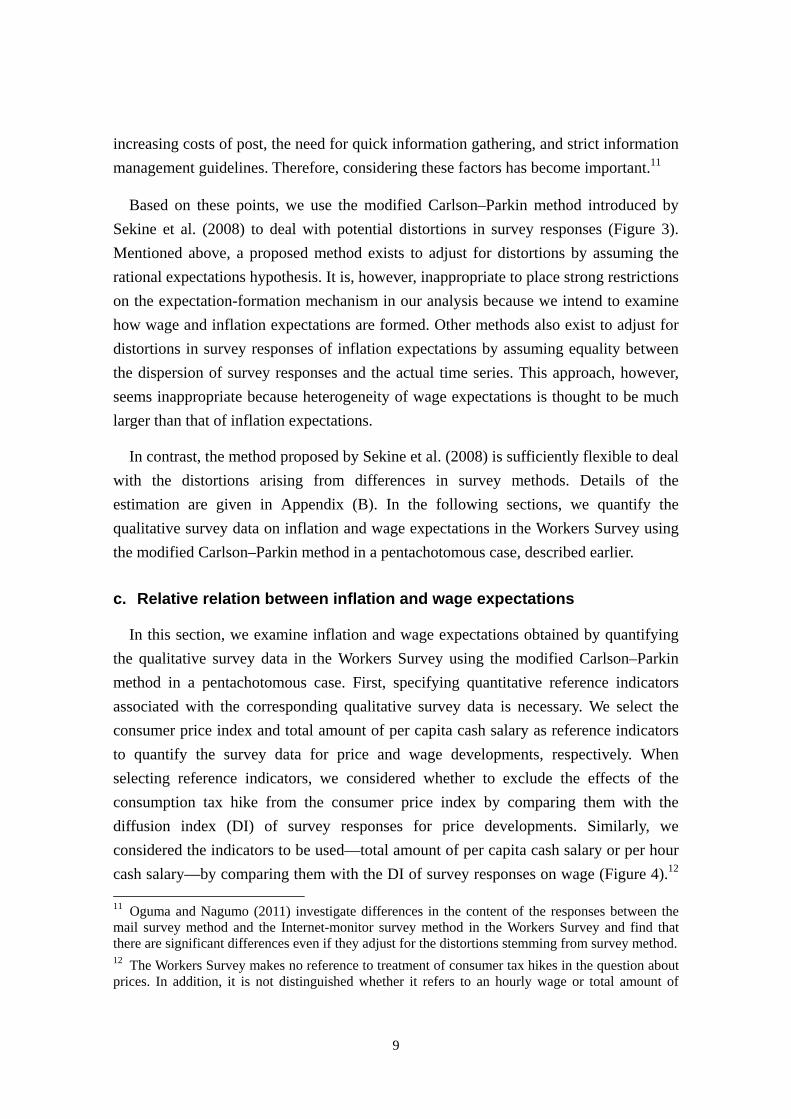
increasing costs of post, the need for quick information gathering, and strict information

management guidelines. Therefore, considering these factors has become important.11

Based on these points, we use the modified Carlson–Parkin method introduced by

Sekine et al. (2008) to deal with potential distortions in survey responses (Figure 3).

Mentioned above, a proposed method exists to adjust for distortions by assuming the

rational expectations hypothesis. It is, however, inappropriate to place strong restrictions

on the expectation-formation mechanism in our analysis because we intend to examine

how wage and inflation expectations are formed. Other methods also exist to adjust for

distortions in survey responses of inflation expectations by assuming equality between

the dispersion of survey responses and the actual time series. This approach, however,

seems inappropriate because heterogeneity of wage expectations is thought to be much

larger than that of inflation expectations.

In contrast, the method proposed by Sekine et al. (2008) is sufficiently flexible to deal

with the distortions arising from differences in survey methods. Details of the

estimation are given in Appendix (B). In the following sections, we quantify the

qualitative survey data on inflation and wage expectations in the Workers Survey using

the modified Carlson–Parkin method in a pentachotomous case, described earlier.

c. Relative relation between inflation and wage expectations

In this section, we examine inflation and wage expectations obtained by quantifying

the qualitative survey data in the Workers Survey using the modified Carlson–Parkin

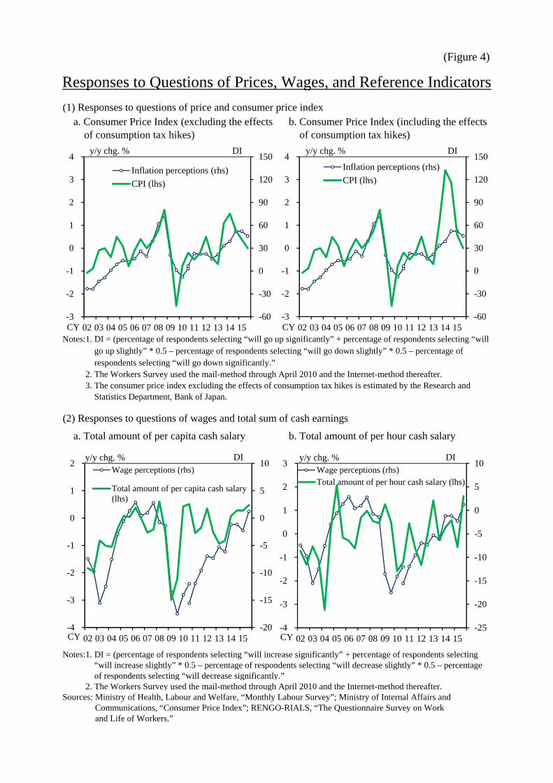
method in a pentachotomous case. First, specifying quantitative reference indicators

associated with the corresponding qualitative survey data is necessary. We select the

consumer price index and total amount of per capita cash salary as reference indicators

to quantify the survey data for price and wage developments, respectively. When

selecting reference indicators, we considered whether to exclude the effects of the

consumption tax hike from the consumer price index by comparing them with the

diffusion index (DI) of survey responses for price developments. Similarly, we

considered the indicators to be used—total amount of per capita cash salary or per hour

cash salary—by comparing them with the DI of survey responses on wage (Figure 4).12 11 Oguma and Nagumo (2011) investigate differences in the content of the responses between the mail survey method and the Internet-monitor survey method in the Workers Survey and find that there are significant differences even if they adjust for the distortions stemming from survey method. 12 The Workers Survey makes no reference to treatment of consumer tax hikes in the question about prices. In addition, it is not distinguished whether it refers to an hourly wage or total amount of

10

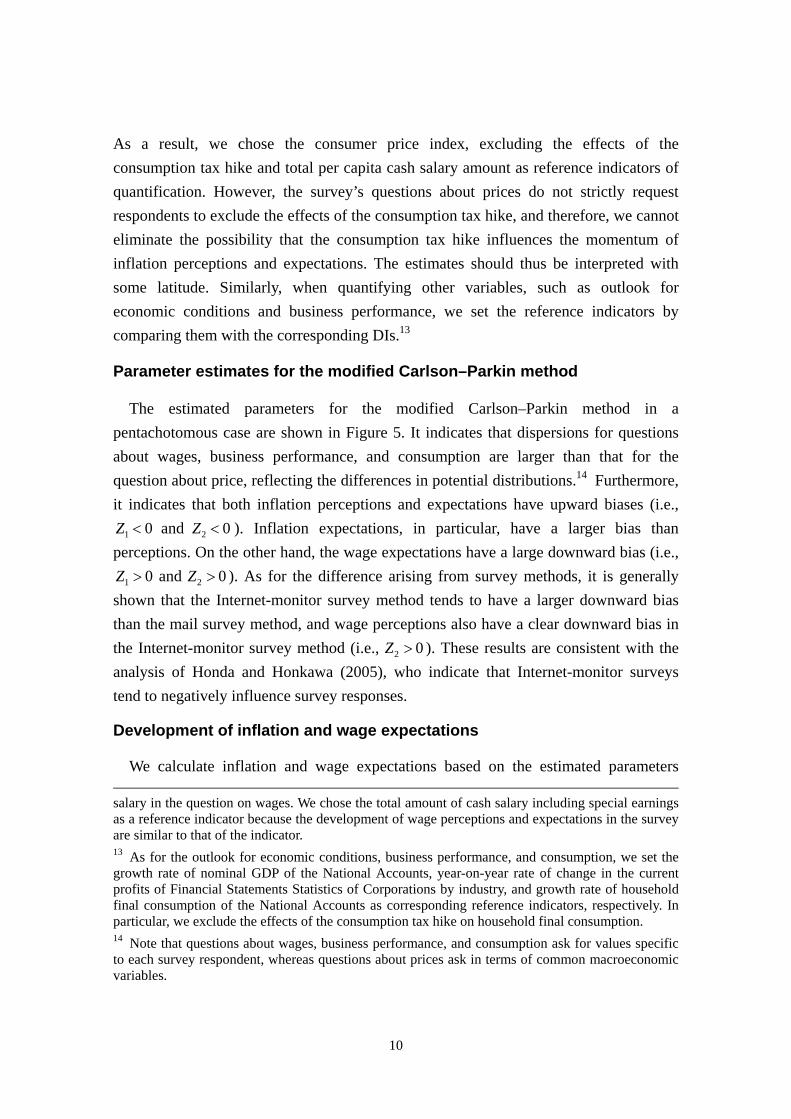
As a result, we chose the consumer price index, excluding the effects of the

consumption tax hike and total per capita cash salary amount as reference indicators of

quantification. However, the survey’s questions about prices do not strictly request

respondents to exclude the effects of the consumption tax hike, and therefore, we cannot

eliminate the possibility that the consumption tax hike influences the momentum of

inflation perceptions and expectations. The estimates should thus be interpreted with

some latitude. Similarly, when quantifying other variables, such as outlook for

economic conditions and business performance, we set the reference indicators by

comparing them with the corresponding DIs.13

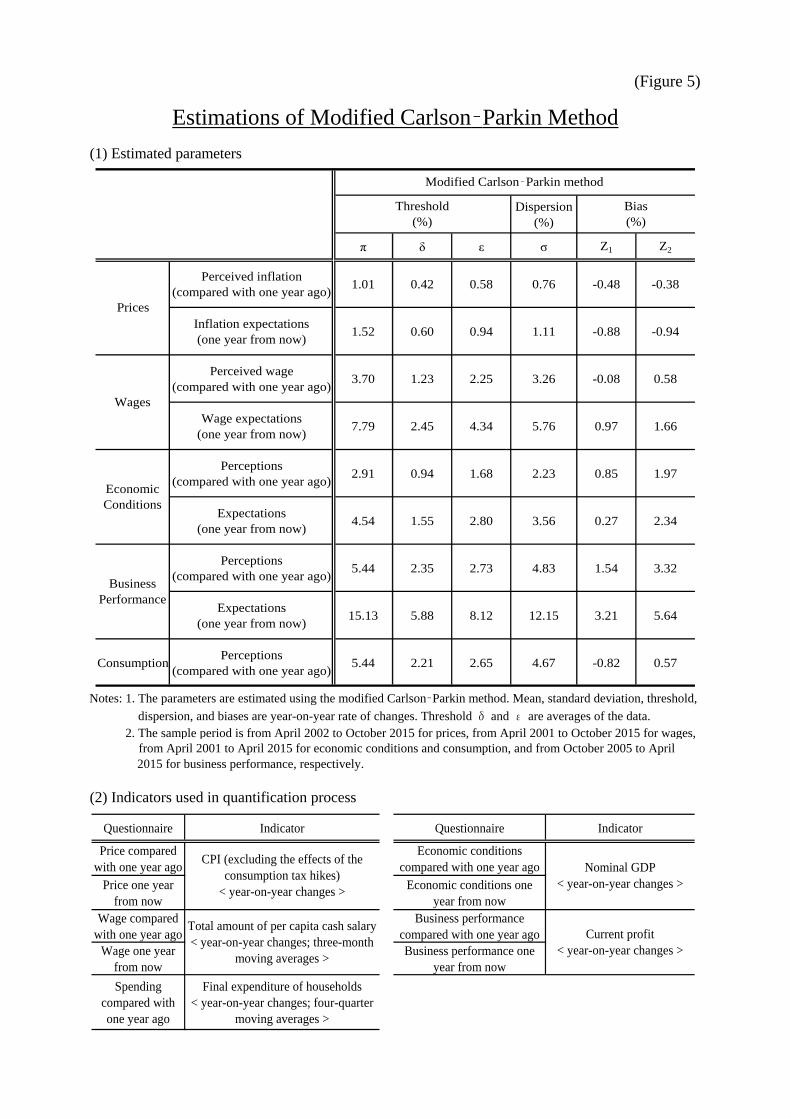
Parameter estimates for the modified Carlson–Parkin method

The estimated parameters for the modified Carlson–Parkin method in a

pentachotomous case are shown in Figure 5. It indicates that dispersions for questions

about wages, business performance, and consumption are larger than that for the

question about price, reflecting the differences in potential distributions.14 Furthermore,

it indicates that both inflation perceptions and expectations have upward biases (i.e.,

01 Z and 02 Z ). Inflation expectations, in particular, have a larger bias than

perceptions. On the other hand, the wage expectations have a large downward bias (i.e.,

01 Z and 02 Z ). As for the difference arising from survey methods, it is generally

shown that the Internet-monitor survey method tends to have a larger downward bias

than the mail survey method, and wage perceptions also have a clear downward bias in

the Internet-monitor survey method (i.e., 02 Z ). These results are consistent with the

analysis of Honda and Honkawa (2005), who indicate that Internet-monitor surveys

tend to negatively influence survey responses.

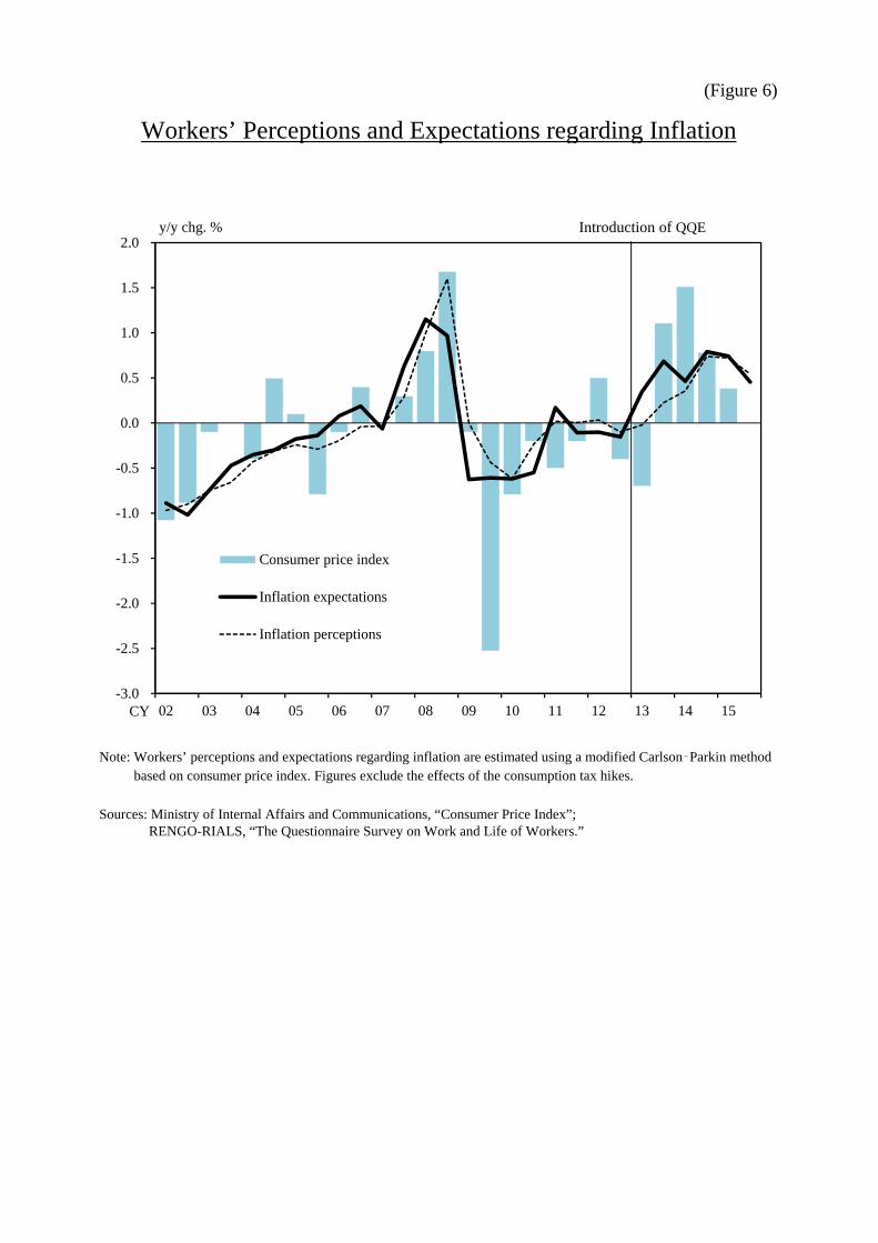
Development of inflation and wage expectations

We calculate inflation and wage expectations based on the estimated parameters salary in the question on wages. We chose the total amount of cash salary including special earnings as a reference indicator because the development of wage perceptions and expectations in the survey are similar to that of the indicator. 13 As for the outlook for economic conditions, business performance, and consumption, we set the growth rate of nominal GDP of the National Accounts, year-on-year rate of change in the current profits of Financial Statements Statistics of Corporations by industry, and growth rate of household final consumption of the National Accounts as corresponding reference indicators, respectively. In particular, we exclude the effects of the consumption tax hike on household final consumption. 14 Note that questions about wages, business performance, and consumption ask for values specific to each survey respondent, whereas questions about prices ask in terms of common macroeconomic variables.

11

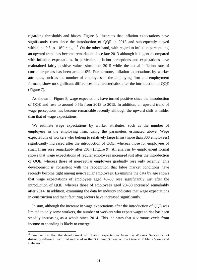
regarding thresholds and biases. Figure 6 illustrates that inflation expectations have

significantly risen since the introduction of QQE in 2013 and subsequently stayed

within the 0.5 to 1.0% range.15 On the other hand, with regard to inflation perceptions,

an upward trend has become remarkable since late 2013 although it is gentle compared

with inflation expectations. In particular, inflation perceptions and expectations have

maintained fairly positive values since late 2015 while the actual inflation rate of

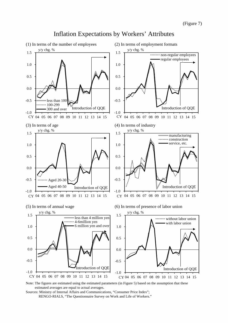
consumer prices has been around 0%. Furthermore, inflation expectations by worker

attributes, such as the number of employees in the employing firm and employment

formats, show no significant differences in characteristics after the introduction of QQE

(Figure 7).

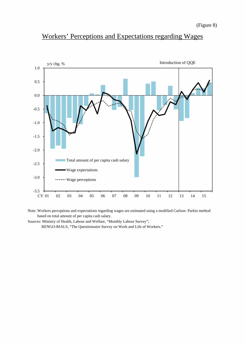
As shown in Figure 8, wage expectations have turned positive since the introduction

of QQE and rose to around 0.5% from 2013 to 2015. In addition, an upward trend of

wage perceptions has become remarkable recently although the upward shift is milder

than that of wage expectations.

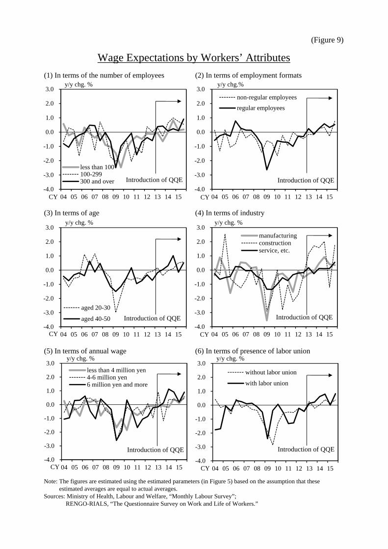
We estimate wage expectations by worker attributes, such as the number of

employees in the employing firm, using the parameters estimated above. Wage

expectations of workers who belong to relatively large firms (more than 300 employees)

significantly increased after the introduction of QQE, whereas those for employees of

small firms rose remarkably after 2014 (Figure 9). An analysis by employment format

shows that wage expectations of regular employees increased just after the introduction

of QQE, whereas those of non-regular employees gradually rose only recently. This

development is consistent with the recognition that labor market conditions have

recently become tight among non-regular employees. Examining the data by age shows

that wage expectations of employees aged 40–50 rose significantly just after the

introduction of QQE, whereas those of employees aged 20–30 increased remarkably

after 2014. In addition, examining the data by industry indicates that wage expectations

in construction and manufacturing sectors have increased significantly.

In sum, although the increase in wage expectations after the introduction of QQE was

limited to only some workers, the number of workers who expect wages to rise has been

steadily increasing as a whole since 2014. This indicates that a virtuous cycle from

income to spending is likely to emerge.

15 We confirm that the development of inflation expectations from the Workers Survey is not distinctly different from that indicated in the “Opinion Survey on the General Public’s Views and Behavior.”

12

Relative relation between inflation and wage expectations

Since the introduction of QQE, both inflation and wage expectations have increased

to some extent. What is the relative relation between those expectations? Burke and

Ozdagli (2013) reveal that consumers, on average, did not expect their wage growth to

match inflation, which would create a negative income effect that discourages spending

in both the present and future. This implies that monitoring the relative relation between

inflation and wage expectations is important.

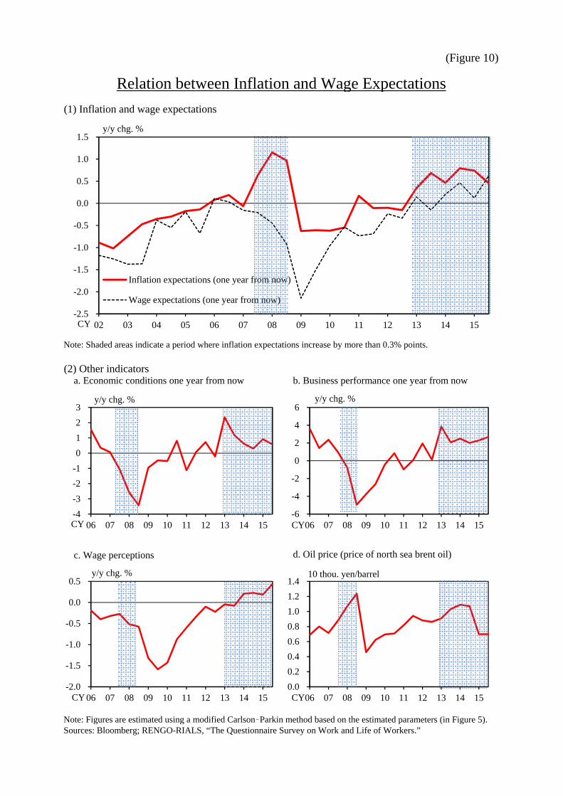
In this section, we investigate the development of inflation and wage expectations,

considering responses to other survey questions (Figure 10). First, when we compare

the rising inflation period in 2007–08 and the period after the introduction of QQE, we

found that wage expectations decreased in the former period but increased in the latter

period. To understand the background, we investigate other survey questions, such as

economic conditions, business performance, and wage perceptions in these two periods.

We then found that those survey responses also improved after the introduction of QQE,

whereas they were sluggish in the 2007–08 period. It is considered that the rise in

inflation expectations in 2007–08 was caused by a commodity price surge in the same

timeframe, with crude oil prices increasing. The effects of rising inflation expectations

in response to cost-push shocks may differ from those of rising inflation expectations

caused by a change in monetary policy, such as the introduction of QQE.

Furthermore, we analyze real wage perceptions and expectations by subtracting

inflation rates from wages in nominal terms (Figure 11). The analysis indicates that real

wage perceptions and expectations decreased to some extent just after the introduction

of QQE because employees did not expect their wage perceptions and expectations to

match inflation.16 In this regard, as Burke and Ozdagli (2013) mentioned, a difference

in the stickiness of inflation and wages may affect this result. However, because wage

expectations have gradually increased recently, real wage expectations have also started

to increase, and the deterioration of wage perceptions has eased. This development is in

stark contrast with the fact that real wage expectations had decreased significantly in

2007–08.

16 Attention should be given to the possibility that the consumption tax hike during the same period has some effects on this estimation.

13

4. Effect of inflation expectations on consumer spending

a. Theoretical background

In theory, the relation between inflation expectations and consumer spending depends

on the relative size of two effects: intertemporal substitution effect and income effect

(Figure 12). On one hand, with nominal interest rates constant, a rise in inflation

expectations decreases real interest rates, which positively impacts consumer spending

by the intertemporal substitution effect through an increase in the relative price of future

goods. In contrast, a decline in inflation expectations negatively impacts consumer

spending, which implies that people defer their consumption through the negative

intertemporal substitution effect in a deepening deflation. Thus, in the process of

overcoming deflation and rising inflation expectations, people are expected to convert

their excessively deferred demand during the deflationary period into effective demand.

On the other hand, a rise in inflation expectations lowers real wage expectations, which

reduces consumer spending by the negative income effect, because it lowers

expectations of real interest rate income through a decrease in real interest rates. In short,

the issue of which effect dominates the other is an empirical matter.

As mentioned above, previous research in Japan (Ichiue and Nishiguchi [2015])

indicates that expectations of a rise in inflation stimulates consumer spending. In

contrast, empirical studies in the US (Burke and Ozdagli [2013], Bachmann et al.

[2015]) show no significant relation between inflation expectations and consumer

spending. Interestingly, recent studies in the US indicate that households, on average,

did not expect their wage growth to match inflation. If this is the case, rising inflation

expectations negatively impact the outlook for real income, which may decrease

consumer spending through the negative income effect.

This section examines the relation between inflation expectations and consumer

spending in Japan, considering changes in wage expectations. We focus on the rising

inflation period in 2007–08 and the period after the introduction of QQE.

b. Estimation model and empirical results

To examine the relation between inflation expectations and consumer spending, we

construct a panel dataset that is age-stratified by five years and quantify qualitative

survey data on perceptions and expectations of inflation, wages, and consumption for

every age stratum, using the modified Carlson–Parkin method in a pentachotomous

14

case. 17 We obtain perceptions and expectations for both real wages and real

consumption, which are adjusted for inflation perceptions and expectations, respectively.

We then conduct a panel analysis based on the age-stratified data using perceptions of

real consumption as a dependent variable and real interest rates, real wage perceptions,

and expectations as explanatory variables. Here, real wage perceptions proxy for recent

development of actual wages. In this estimation, we consider several models with

different lag structures and control for the age groups.

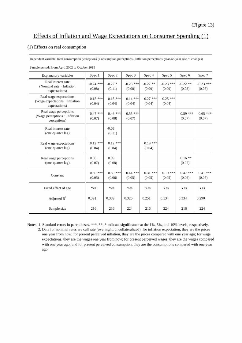
For each model, the signs of the regression coefficients are consistent with our

expectations, and the estimation result indicates that lowering real interest rates

increases perceptions of real consumption (Figure 13). This empirical result indicates

that rising inflation expectations positively impact consumer spending through a

decrease in real interest rates, with constant nominal interest rates.

As mentioned in studies for the US, however, rising inflation expectations may

negatively impact consumer spending when a rise in wage expectations does not catch

up with that of inflation expectations; as a result, real wage expectations decrease. In

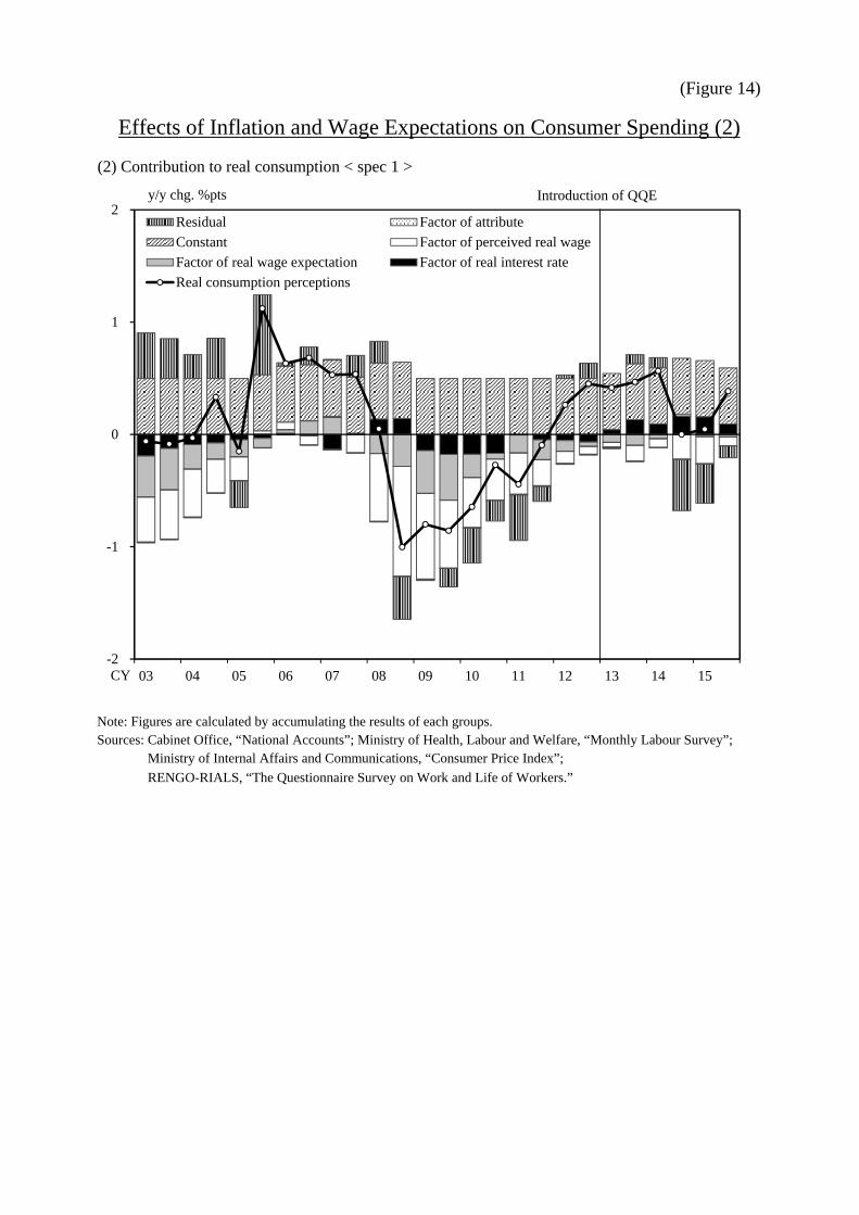
this regard, we examine the background to the development of perceptions of real

consumption in both the rising inflation period of 2007–08 and the period after the

introduction of QQE (Figure 14). As for the 2007–08 period, the negative effects of

declining real wage expectations are larger than the positive effect of falling real interest

rates; as a result, a rise in inflation expectations reduces consumer spending after all. On

the other hand, the positive effect of falling real interest rates dominates the negative

effect of lowering real wage expectations after the introduction of QQE, and as a result,

the rise in inflation expectations stimulates consumer spending on the whole.

Reflecting these results, it is thought that whether a rise in inflation expectations with

low and stable nominal interest rates will positively impact consumer spending depends

on the relative relation between inflation and wage expectations, which may vary over

time. We then examine the development of real consumption after the introduction of

QQE. The analysis reveals that a decline in real wages has been limited, reflecting a

mild increase in wage expectations even under rising inflation expectations. Therefore,

a rise in inflation expectations after the introduction of QQE positively impacts

17 It is appropriate to select the reference indicators for the corresponding age groups respectively. However, due to data limitations, we select the reference indicators which are used in the full sample estimation (i.e., consumer price index, total amount of cash salary, and household final consumption).

15

consumption on the whole. This result enables us to conjecture that households have

gradually converted their excessively deferred demand during deflation into effective

demand through the positive intertemporal substitution effect.

The analysis also shows that real wage perceptions have persistently depressed

consumption over the period of interest. In the next section, we investigate the relation

between wage perceptions and expectations.

5. Formation mechanism of wage expectations

a. Framework of analysis

As mentioned in the previous section, rising inflation expectations positively impact

consumer spending when both wage and inflation expectations increase in a balanced

way. Here, the question is what determines wage expectations? In this section, we

perform an empirical analysis using the data from the Workers Survey to answer this

question.

Specifically, we conduct a panel data analysis using wage expectations as a

dependent variable with other indexes obtained from the Workers Survey, such as

perceptions and expectations of inflation, wages, economic conditions, and business

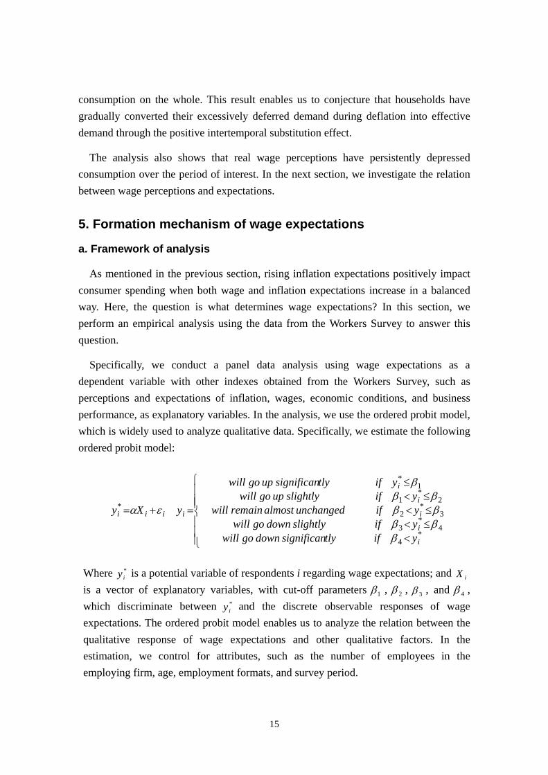
performance, as explanatory variables. In the analysis, we use the ordered probit model,

which is widely used to analyze qualitative data. Specifically, we estimate the following

ordered probit model:

　

　　　　　　　　

　　　　　　　　　　

　　　　　

　　　　　　　　　　　

　　　　　　　　

　

*4

4*

3

3*

2

2*

1

1*

*

i

i

i

i

i

iiii

yiftlysignificandowngowillyifslightlydowngowillyifunchangedalmostremainwillyifslightlyupgowill

yiftlysignificanupgowill

yXy

Where *iy

is a potential variable of respondents i regarding wage expectations; and iX

is a vector of explanatory variables, with cut-off parameters 1 , 2 , 3 , and 4 ,

which discriminate between *iy

and the discrete observable responses of wage

expectations. The ordered probit model enables us to analyze the relation between the

qualitative response of wage expectations and other qualitative factors. In the

estimation, we control for attributes, such as the number of employees in the

employing firm, age, employment formats, and survey period.

16

b. Empirical results

Mechanism through which wage expectations are formed

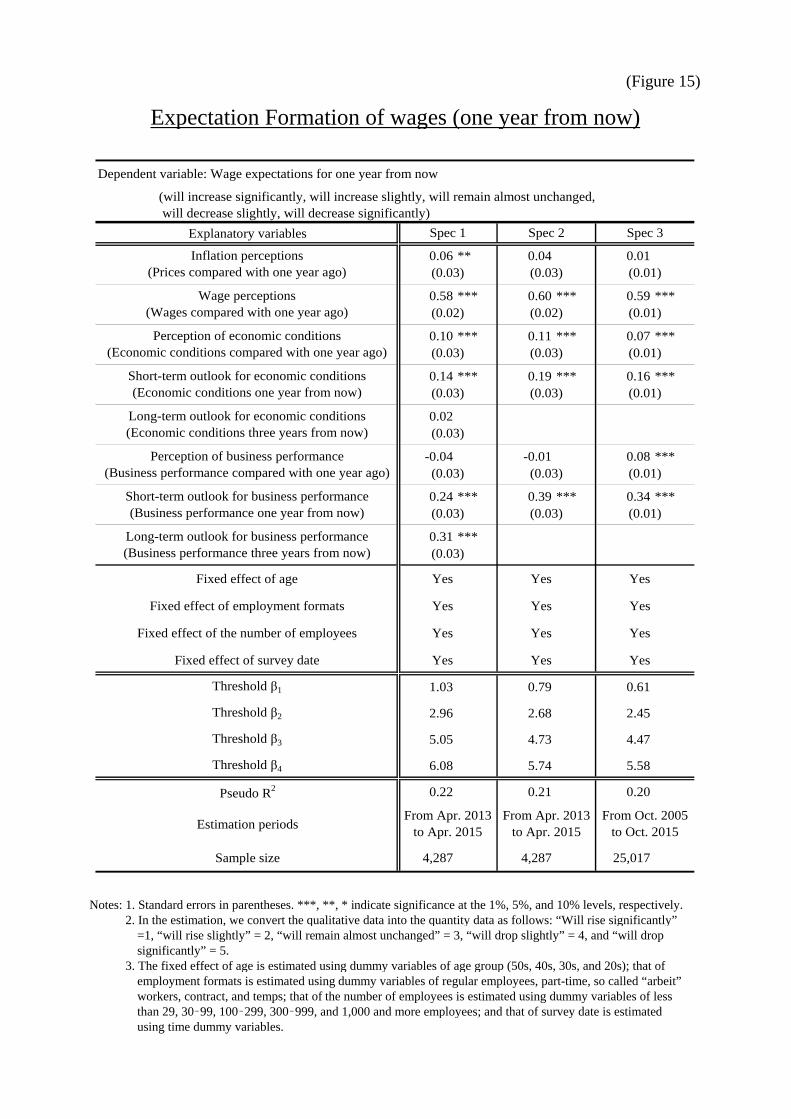
First, we estimate the ordered probit model using wage expectations for one year

from now as a dependent variable. In the estimation, we examine several specifications

as shown in Figure 15.18 The estimation results indicate that wage expectations are

significantly affected by perceptions of wages and economic conditions, outlook for

economic conditions, and business performance in all specifications.19 In particular,

coefficient size tells us that both wage perceptions and outlook for business

performance significantly impact wage expectations. This indicates that wage

expectations are formed in both a forward-looking and backward-looking manner. On

the other hand, the effect of inflation perceptions is modest in the sense that statistical

significance is obtained only for part of the specifications,20 with the coefficients

smaller than those on wage perceptions and outlook for business performance.

In summary, a rise in wage expectations necessitates an increase in actual wages and

an improvement in business performance outlook. In the face of rising inflation in

2007–08, wage expectations did not increase in circumstances where the outlook for

economic conditions and business performance failed to improve. An increase in actual

wages is important for wage expectations to rise significantly in tandem with inflation

expectations.

Next, we turn to wage expectations for three and five years from now. Figure 16

shows that they are significantly affected by outlook for economic conditions and

business performance as well as by wage perceptions, which is consistent with the

estimation result for wage expectations for one year from now. Considering the

coefficient sizes in detail, wage perceptions and economic conditions seems less

effective, whereas long-term outlooks for economic conditions and business

performance seem more effective, compared with the case of wage expectations for one

year from now. This result indicates that an improvement in forward-looking factors,

18 The Workers Survey started collecting long-term data in April 2013. This long-term data includes the three-year outlook for inflation, economic conditions, and business performance as well as three- and five-year outlook for wages. 19 In the estimation, we control for attributes such as the number of employees in the employing

firm, age, employment formats, and survey period, using dummy variables. 20 The result is consistent with the fact that the development of current inflation is taken into account in the wage-setting process between employees and employers in Japan.

17

such as wage expectations and outlook for business performance, is important for

long-term wage expectations to rise.

Characteristics observed for workers’ attributes

Do determinants of wage expectations differ according to worker attributes?

Intuitively, regular employees are thought to form wage expectations differently from

non-regular employees due to differences in their respective payroll systems.

In this section, we analyze the effects of workers’ attributes, such as employment

formats and presence of labor unions, on wage expectations by adding interaction terms

into the ordered probit model as independent variables. As for employment formats, for

example, we construct dummy variables that take the value of unity for regular

employees and zero otherwise. We then construct interaction terms by multiplying all

independent variables in the probit model by the corresponding dummy variables.

Examining the estimated coefficients on the interaction terms enables us to investigate

the effects of employment format on wage expectations.21

Figure 17 shows the interaction terms of employment formats, indicating that wage

expectations of regular employees are more significantly affected by wage perceptions

than those of non-regular employees. This result may imply that regular employees tend

to expect their wages to be stable over time, reflecting their perceptions of greater job

security than non-regular workers.

Next, we investigate the effect of the presence of labor unions on wage expectations

(Figure 18). The analysis reveals that employees who work at firms with a labor union

significantly tend to expect higher wages when they hold a good business performance

outlook. This result indicates the possibility that workers who work for firms with a

labor union have a tendency to expect their wages to increase through labor unions’

negotiating power when perceiving improvements in business performance.

6. Conclusion

This paper uses micro data from the Workers Survey conducted by RENGO-RIALS

to investigate the effects of inflation expectations on consumer spending, considering

changes in wage expectations.

21 In this section, we analyze workers working at large firms with more than 100 employees in order to control for firm size.

18

In the analysis, we use the modified Carlson–Parkin method in a pentachotomous

case to deal with five-choice questionnaires and potential distortions of survey

responses in the Workers Survey. We then quantify qualitative survey data on inflation

and wage expectations. The estimation result reveals that wage expectations have

moderately risen since the introduction of QQE. In particular, the number of workers

who expect wages to rise has been steadily increasing as a whole since 2014, which

indicates that a virtuous cycle from income to spending is likely to emerge.

Furthermore, we analyze the effect of expectations of rising inflation on consumer

spending after the introduction of QQE, considering changes in wage expectations. The

estimation result shows that the positive effect of falling real interest rates on consumer

spending is larger than the negative effect of a decline in real wage expectations after the

introduction of QQE; as a result, a rise in inflation expectations stimulates consumer

spending.

Then, we used the ordered probit model to analyze the relation between wage

expectations and other survey responses to investigate the mechanism through which

wage expectations are formed. The result indicates that wage expectations are strongly

influenced by wage perceptions and outlook for business performance, implying that an

improvement in forward-looking factors, such as wage expectations and business

performance outlook, is important for long-term wage expectations to rise.

Finally, attention should be given to the limitations of the analysis presented above.

This paper employs the Carlson–Parkin method to measure inflation and wage

expectations. The Carlson–Parkin method requires several strong assumptions regarding

the shape of the respondents’ distribution, constancy of thresholds, and long-term

equality between perceived and expected values, in addition to the selection of reference

indicators. Therefore, some errors may arise in the estimation of inflation and wage

expectations. It is also possible that we failed to control for the effects of a consumption

tax hike on the estimation due to data constraints. With these considerations, we would

like to emphasize that all the estimates given in this paper should be interpreted with

some latitude.

19

Appendix. Estimation method of inflation and wage expectations

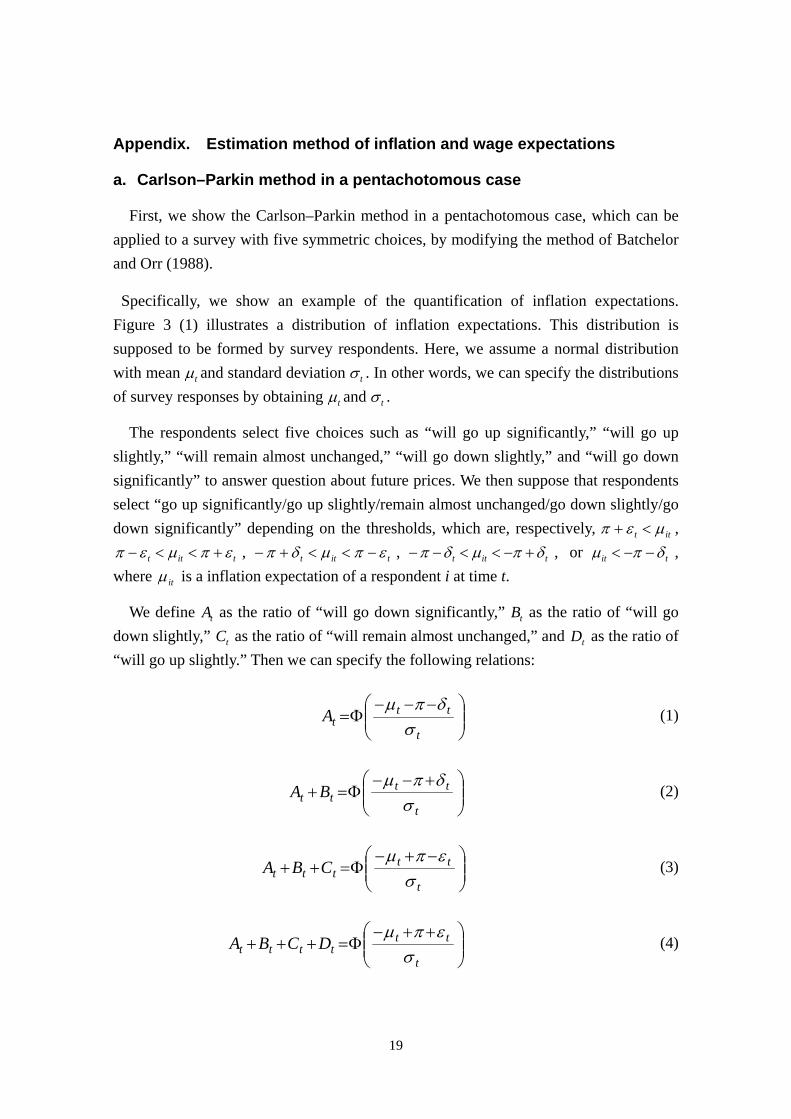
a. Carlson–Parkin method in a pentachotomous case

First, we show the Carlson–Parkin method in a pentachotomous case, which can be

applied to a survey with five symmetric choices, by modifying the method of Batchelor

and Orr (1988).

Specifically, we show an example of the quantification of inflation expectations.

Figure 3 (1) illustrates a distribution of inflation expectations. This distribution is

supposed to be formed by survey respondents. Here, we assume a normal distribution

with mean t and standard deviation t . In other words, we can specify the distributions

of survey responses by obtaining t and t .

The respondents select five choices such as “will go up significantly,” “will go up

slightly,” “will remain almost unchanged,” “will go down slightly,” and “will go down

significantly” to answer question about future prices. We then suppose that respondents

select “go up significantly/go up slightly/remain almost unchanged/go down slightly/go

down significantly” depending on the thresholds, which are, respectively, itt ,

titt , titt , titt , or tit ,

where it is a inflation expectation of a respondent i at time t.

We define tA as the ratio of “will go down significantly,” tB as the ratio of “will go

down slightly,”

tC as the ratio of “will remain almost unchanged,” and tD as the ratio of

“will go up slightly.” Then we can specify the following relations:

t

tttA

(1)

t

tttt BA

(2)

t

ttttt CBA

(3)

t

tttttt DCBA

(4)

20

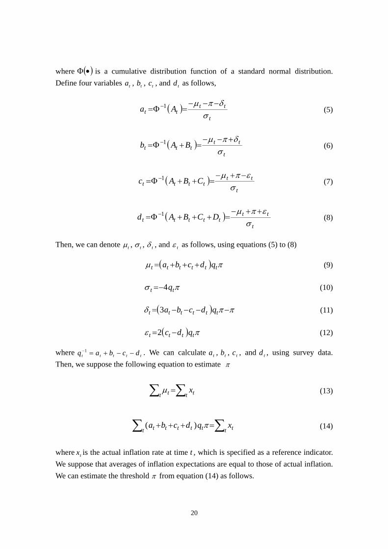
where is a cumulative distribution function of a standard normal distribution.

Define four variables ta , tb , tc , and td as follows,

t

tttt Aa

1

(5)

t

ttttt BAb

1 (6)

t

tttttt CBAc

1 (7)

t

ttttttt DCBAd

1 (8)

Then, we can denote t , t , t , and t as follows, using equations (5) to (8)

tttttt qdcba (9)

tt q4 (10)

tttttt qdcba3 (11)

tttt qdc 2 (12)

where ttttt dcbaq 1 . We can calculate ta , tb , tc , and td , using survey data.

Then, we suppose the following equation to estimate

t tt t x (13)

t tt ttttt xqdcba )( (14)

where tx is the actual inflation rate at time t , which is specified as a reference indicator.

We suppose that averages of inflation expectations are equal to those of actual inflation.

We can estimate the threshold from equation (14) as follows.

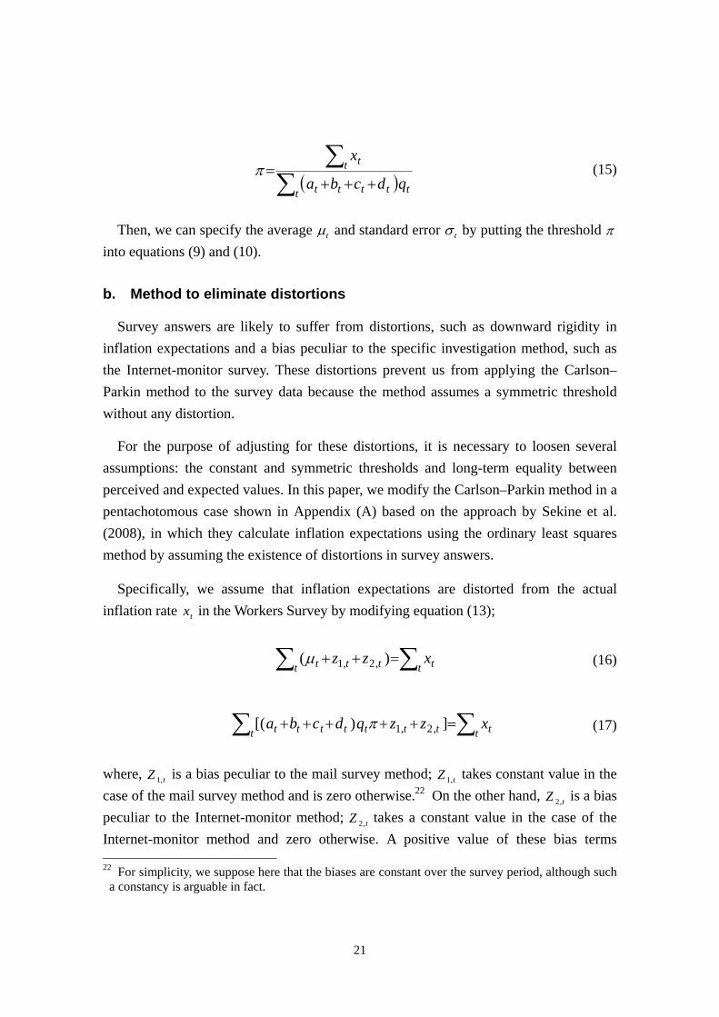
21

t ttttt

t t

qdcba

x (15)

Then, we can specify the average t and standard error

t by putting the threshold

into equations (9) and (10).

b. Method to eliminate distortions

Survey answers are likely to suffer from distortions, such as downward rigidity in

inflation expectations and a bias peculiar to the specific investigation method, such as

the Internet-monitor survey. These distortions prevent us from applying the Carlson–

Parkin method to the survey data because the method assumes a symmetric threshold

without any distortion.

For the purpose of adjusting for these distortions, it is necessary to loosen several

assumptions: the constant and symmetric thresholds and long-term equality between

perceived and expected values. In this paper, we modify the Carlson–Parkin method in a

pentachotomous case shown in Appendix (A) based on the approach by Sekine et al.

(2008), in which they calculate inflation expectations using the ordinary least squares

method by assuming the existence of distortions in survey answers.

Specifically, we assume that inflation expectations are distorted from the actual

inflation rate tx in the Workers Survey by modifying equation (13);

t tt ttt xzz )( ,2,1 (16)

t tt ttttttt xzzqdcba ])[( ,2,1 (17)

where, tZ ,1

is a bias peculiar to the mail survey method; tZ ,1 takes constant value in the

case of the mail survey method and is zero otherwise.22 On the other hand, tZ ,2

is a bias

peculiar to the Internet-monitor method; tZ ,2 takes a constant value in the case of the

Internet-monitor method and zero otherwise. A positive value of these bias terms 22 For simplicity, we suppose here that the biases are constant over the survey period, although such

a constancy is arguable in fact.

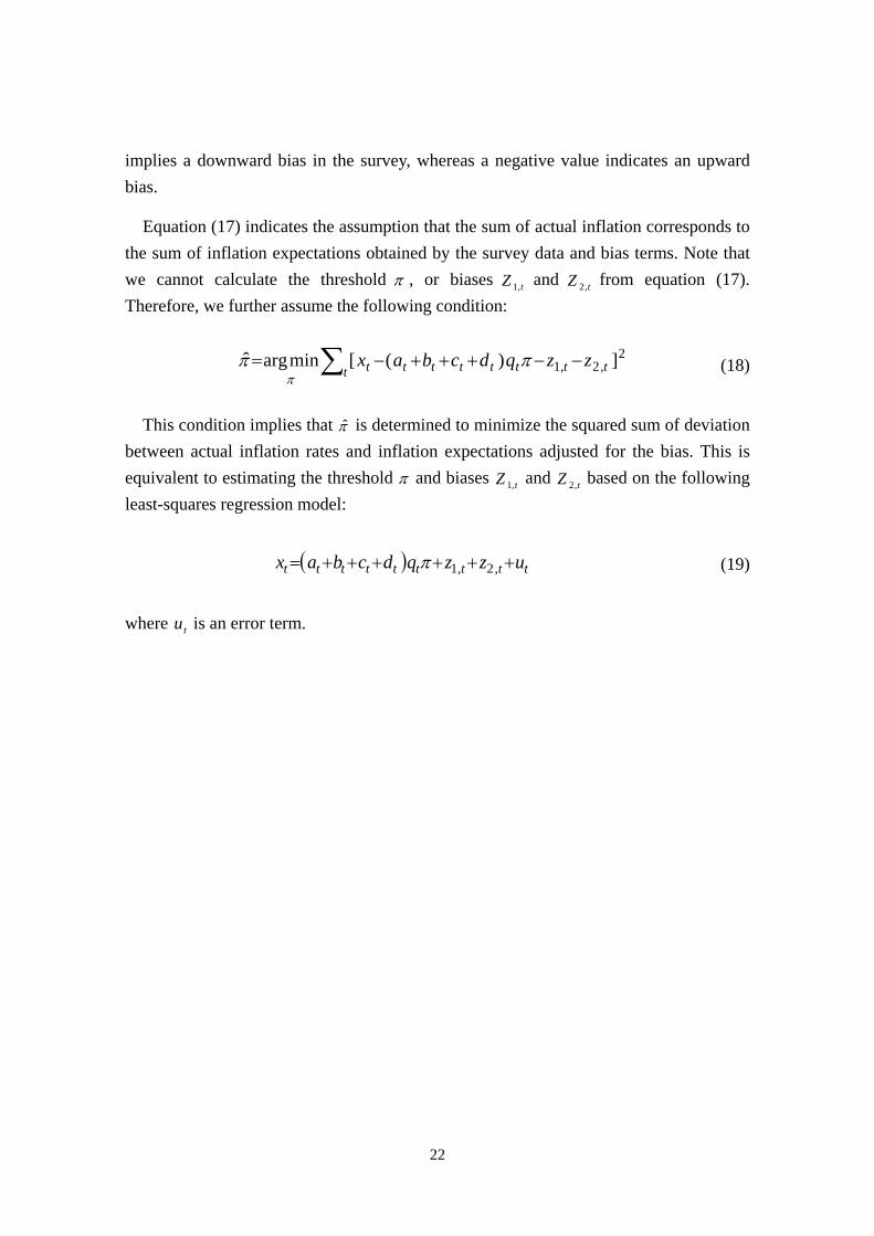
22

implies a downward bias in the survey, whereas a negative value indicates an upward

bias.

Equation (17) indicates the assumption that the sum of actual inflation corresponds to

the sum of inflation expectations obtained by the survey data and bias terms. Note that

we cannot calculate the threshold , or biases tZ ,1 and tZ ,2 from equation (17).

Therefore, we further assume the following condition:

t tttttttt zzqdcbax 2

,2,1 ])([minargˆ

(18)

This condition implies that ̂ is determined to minimize the squared sum of deviation

between actual inflation rates and inflation expectations adjusted for the bias. This is

equivalent to estimating the threshold and biases tZ ,1 and tZ ,2

based on the following

least-squares regression model:

ttttttttt uzzqdcbax ,2,1 (19)

where tu is an error term.

23

References

Bachmann, R., Tim O. Berg, and Eric R. Sims, “Inflation Expectations and Readiness to

Spend: Cross-Sectional Evidence,” Economic Policy, vol. 7 No. 1, 2015, pp. 1–35.

Batchelor, R. A. and A. B. Orr, “Inflation Expectations Revisited,” Economica, vol. 55

No. 219, 1988, pp. 317-331.

Bernanke, Ben S., “Inflation Expectations and Inflation Forecasting,” Speech at the

Monetary Economics Workshop of the National Bureau of Economic Research

Summer Institute, Cambridge, Massachusetts, July 10, 2007.

Bruine de Bruin, W., S. Potter, R. Rich, G. Topa and W. van der Klaauw, “Improving

Survey Measures of Household Inflation Expectations,” Current Issues in

Economics and Finance, Vol. 16 No. 7, Aug/Sept 2010.

Burke, M. A. and A. K. Ozdagli, “Household Inflation Expectations and Consumer

Spending: Evidence from Panel Data.” Working Paper No. 13-25, Federal Reserve

Bank of Boston, 2013.

Carlson, J. A. and M. Parkin, “Inflation Expectation,” Economica, vol. 42, 1975, pp.

123-138.

D’Acunto, F., D. Hoang, and M. Weber, “Inflation Expectations and Consumption

Expenditure,” Working paper, Chicago Booth Global Markets, 2015.

Honda, N. and A. Honkawa, “Internet chousa ha syakai chousa ni riyou dekiru ka (Can

We Use an Internet Survey in the Social Study?),” Roudouseisaku kenkyu

houkokusyo, No. 17, roudou seisaku kenkyu kenshu kikou, 2005, in Japanese.

Hori, M. and A. Terai, “Carlson-Parkin hou niyoru infure kitai no keisoku to syomondai

(Measurement of Inflation Expectations by the Carlson–Parkin Method and Its

Problems),” Keizaibunseki, No. 175, pp. 167-173, 2005, in Japanese.

Ichiue, H. and S. Nishiguchi, “Inflation Expectations and Consumer Spending at the

Zero Bound: Micro Evidence,” Economic Inquiry, Vol. 53 No. 2, 2015, pp. 1086–

1107.

Kamada, K., “Downward Rigidity in Households’ Price Expectations: An analysis

Based on the Bank of Japan’s ‘Opinion Survey on the General Public’s Views and

24

Behavior’”, Bank of Japan Working Paper Series, No. 13-E-15, 2013.

Kamada, K., J. Nakajima and S. Nishiguchi, “Are Household Inflation Expectations

Anchored in Japan?” Bank of Japan Working Paper Series, No. 15-E-8, 2015.

Kano, S., “Macro keizai bunseki to survey data (Macroeconomic Analysis Using Survey

Data)”, Iwanami shoten, 2006, in Japanese.

Nielsen, H., “Inflation Expectations in the EU: Results from Survey Data,” Discussion

papers of interdisciplinary research project 373, No. 13, 2003.

Nishiguchi, S., J. Nakajima, and K. Imakubo, “Disagreement in Households’ Inflation

Expectations and Its Evolution,” Bank of Japan Review Series, No. 14-E-1, 2014.

Oguma, S. and C. Nagumo, “Shakai-chousa ni okeru internet-monitor chousa to

yusou-monitor chousa tono hikaku (Comparison of Internet-Monitor Survey Method and

Mail Survey Method in Social Survey),” Rengo souken report No. 258, pp. 20-27, Rengo

souken, 2011, in Japanese.

Oguma, S. and C. Nagumo, “Kinrousha ga kakaeru shitsugyou to seikatsu no fuan (Fear of

Job Loss and Poverty among Workers),” Nihon roudou kenkyu zashi, No. 612, pp. 29-39,

2011, in Japanese.

Potter, S., “Improving Survey Measures of Inflation Expectations,” Speech at

Forecasters Club of New York, March 30, 2011.

Sekine, T., K. Yoshimura, and C. Wada, “Infureyosou ni tsuite (Inflation Expectations),”

Bank of Japan Review Series, No. 08-J-15, 2008, in Japanese.

Van der Klaauw, W., W. Bruine de Bruin, G. Topa, S. Potter, and M. F. Bryan,

“Rethinking the Measurement of Household Inflation Expectations: Preliminary

Findings,” Federal Reserve Bank of New York Staff Report, No. 359, 2008.

(Figure 1)

Sources: Cabinet Office, “Consumer Confidence Survey”; RENGO-RIALS, “The Questionnaire Survey on Work andSources: Life of Workers”; BOJ, “Opinion Survey on the General Public’s Views and Behavior.”

Details of Workers Survey

Survey Conductor RENGO-RIALS Bank of Japan Cabinet Office

TargetPeople working in private firms

(in Tokyo or Kansai metropolitanarea)

Individuals who are atleast 20 years of age

Households of two ormore persons/one-person households

Population(Statistics to be

Based on)

Workers(on the Employment Status Survey)

Households(on the Resident

Registration System)

Households(on the Population

Census)

Sample Size2,000

(in Oct. 2015)2,122

(in Dec. 2015)5,493

(in Dec. 2015)

Starting Year ofthe Survey

2001 1993 1957

FrequencySemi-annually

(in April/October)Quarterly Monthly

Questionnaire onIncome

Wage (present)Wage (next year)

Household income (present)Household income (next year)

Household income(present)

Household income(next year)

Household income(six months later)

Workers’Attributes

Industry, employment formats,the number of employees,

occupation,the length of service,

presence of labor union, etc.

Occupation(full-time or part-time,

etc.)

Occupation(farmer or worker, etc.)

Individuals’Attributes

Sex, age, income, education,marital status, region, etc.

Sex, age, income, familytype, region, etc.

Sex, age, income,region, scale city, etc.

OtherQuestionnaire

Economy, business performance,price, a circumstance of life,

consumption expenditure, etc.

Business confidence, acircumstance of life,

expenditure, price, landprice, recognition of BOJ’s

objectives, etc.

A circumstance of life,willingness to buy

durable goods, price,etc.

Workers SurveyOpinion Survey on theGeneral Public's Views

and Behavior

Consumer ConfidenceSurvey

(Figure 2)

(1) Carlson–Parkin method (Conceptual diagram)

Carlson–Parkin Method (Conceptual Diagram)

Density

0 Threshold

Average= observed inflation expectations

Will remain almost unchanged

Will go up

Will go down

(Figure 3)

(1) Underlying distribution in the Carlson–Parkin method in a pentachotomous case

(2) Adjustment for biases

Modified Carlson–Parkin Method in a Pentachotomous Case

a. The mail survey method b. The Internet-monitor survey method

Will go down significantly

Will go down slightly

Threshold

Density

Will remain almost unchanged

Will go up slightly

Will go up significantly

Average= observed inflation expectations

0+ +

Threshold

Density

Underlying distribution

Distribution of survey answers

Bias (Z1)

+Z1

Distribution of survey answers

Threshold

Density

+Z2

Bias (Z2)Underlying distribution

(Figure 4)

(1) Responses to questions of price and consumer price index

Notes:1. DI = (percentage of respondents selecting “will go up significantly” + percentage of respondents selecting “will Notes:1. go up slightly” * 0.5 – percentage of respondents selecting “will go down slightly” * 0.5 – percentage ofNotes:1. respondents selecting “will go down significantly.”Notes:2. The Workers Survey used the mail-method through April 2010 and the Internet-method thereafter.Notes:3. The consumer price index excluding the effects of consumption tax hikes is estimated by the Research andNotes:3. Statistics Department, Bank of Japan.

Notes:1. DI = (percentage of respondents selecting “will increase significantly” + percentage of respondents selectingNotes:1. “will increase slightly” * 0.5 – percentage of respondents selecting “will decrease slightly” * 0.5 – percentageNotes:1. of respondents selecting “will decrease significantly.”Notes:2. The Workers Survey used the mail-method through April 2010 and the Internet-method thereafter.Sources: Ministry of Health, Labour and Welfare, “Monthly Labour Survey”; Ministry of Internal Affairs and Sources: Communications, “Consumer Price Index”; RENGO-RIALS, “The Questionnaire Survey on WorkSources: and Life of Workers.”

Responses to Questions of Prices, Wages, and Reference Indicators

a. Consumer Price Index (excluding the effects of consumption tax hikes)

b. Consumer Price Index (including the effects of consumption tax hikes)

a. Total amount of per capita cash salary b. Total amount of per hour cash salary

(2) Responses to questions of wages and total sum of cash earnings

02 03 04 05 06 07 08 09 10 11 12 13 14 15-3

-2

-1

0

1

2

3

4

-60

-30

0

30

60

90

120

150

Inflation perceptions (rhs)

CPI (lhs)

y/y chg. %

CY

DI

02 03 04 05 06 07 08 09 10 11 12 13 14 15-4

-3

-2

-1

0

1

2

-20

-15

-10

-5

0

5

10Wage perceptions (rhs)

Total amount of per capita cash salary(lhs)

DI

CY

y/y chg. %

02 03 04 05 06 07 08 09 10 11 12 13 14 15-4

-3

-2

-1

0

1

2

3

-25

-20

-15

-10

-5

0

5

10Wage perceptions (rhs)Total amount of per hour cash salary (lhs)

DIy/y chg. %

CY

02 03 04 05 06 07 08 09 10 11 12 13 14 15-3

-2

-1

0

1

2

3

4

-60

-30

0

30

60

90

120

150Inflation perceptions (rhs)

CPI (lhs)

CY

DIy/y chg. %

(Figure 5)

(1) Estimated parameters

Notes: 1. The parameters are estimated using the modified Carlson–Parkin method. Mean, standard deviation, threshold,

Notes: 1 .dispersion, and biases are year-on-year rate of changes. Threshold δ and ε are averages of the data.Notes: 2. The sample period is from April 2002 to October 2015 for prices, from April 2001 to October 2015 for wages, otes: 2. from April 2001 to April 2015 for economic conditions and consumption, and from October 2005 to April 2015 for business performance, respectively.

(2) Indicators used in quantification process

Estimations of Modified Carlson–Parkin Method

Dispersion(%)

π δ ε σ Z1 Z2

Perceived inflation(compared with one year ago)

1.01 0.42 0.58 0.76 -0.48 -0.38

Inflation expectations(one year from now)

1.52 0.60 0.94 1.11 -0.88 -0.94

Perceived wage(compared with one year ago)

3.70 1.23 2.25 3.26 -0.08 0.58

Wage expectations(one year from now)

7.79 2.45 4.34 5.76 0.97 1.66

Perceptions(compared with one year ago)

2.91 0.94 1.68 2.23 0.85 1.97

Expectations(one year from now)

4.54 1.55 2.80 3.56 0.27 2.34

Perceptions(compared with one year ago)

5.44 2.35 2.73 4.83 1.54 3.32

Expectations(one year from now)

15.13 5.88 8.12 12.15 3.21 5.64

ConsumptionPerceptions

(compared with one year ago)5.44 2.21 2.65 4.67 -0.82 0.57

EconomicConditions

BusinessPerformance

Prices

Modified Carlson‐Parkin method

Wages

Threshold(%)

Bias(%)

Questionnaire Indicator Questionnaire Indicator

Price comparedwith one year ago

Economic conditionscompared with one year ago

Price one yearfrom now

Economic conditions oneyear from now

Wage comparedwith one year ago

Business performancecompared with one year ago

Wage one yearfrom now

Business performance oneyear from now

Spendingcompared withone year ago

Final expenditure of households< year-on-year changes; four-quarter

moving averages >

CPI (excluding the effects of theconsumption tax hikes)

< year-on-year changes >

Total amount of per capita cash salary< year-on-year changes; three-month

moving averages >

Current profit< year-on-year changes >

Nominal GDP< year-on-year changes >

(Figure 6)

Note: Workers’ perceptions and expectations regarding inflation are estimated using a modified Carlson–Parkin methodNote: based on consumer price index. Figures exclude the effects of the consumption tax hikes.

Sources: Ministry of Internal Affairs and Communications, “Consumer Price Index”; RENGO-RIALS, “The Questionnaire Survey on Work and Life of Workers.”

Workers’ Perceptions and Expectations regarding Inflation

-3.0

-2.5

-2.0

-1.5

-1.0

-0.5

0.0

0.5

1.0

1.5

2.0

02 03 04 05 06 07 08 09 10 11 12 13 14 15

Consumer price index

Inflation expectations

Inflation perceptions

y/y chg. %

CY

Introduction of QQE

(Figure 7)

(1) In terms of the number of employees (2) In terms of employment formats

(3) In terms of age (4) In terms of industry

(5) In terms of annual wage (6) In terms of presence of labor union

Note: The figures are estimated using the estimated parameters (in Figure 5) based on the assumption that theseNote: estimated averages are equal to actual averages.Sources: Ministry of Internal Affairs and Communications, “Consumer Price Index”; RENGO-RIALS, “The Questionnaire Survey on Work and Life of Workers.”

Inflation Expectations by Workers’ Attributes

-1.0

-0.5

0.0

0.5

1.0

1.5

04 05 06 07 08 09 10 11 12 13 14 15

less than 100100-299300 and over

CY

y/y chg. %

Introduction of QQE-1.0

-0.5

0.0

0.5

1.0

1.5

04 05 06 07 08 09 10 11 12 13 14 15

non-regular employeesregular employees

CY

y/y chg. %

Introduction of QQE

-1.0

-0.5

0.0

0.5

1.0

1.5

04 05 06 07 08 09 10 11 12 13 14 15

Aged 20-30

Aged 40-50

CY

y/y chg. %

Introduction of QQE-1.0

-0.5

0.0

0.5

1.0

1.5

04 05 06 07 08 09 10 11 12 13 14 15

manufacturingconstructionservice, etc.

y/y chg. %

CY

Introduction of QQE

-1.0

-0.5

0.0

0.5

1.0

1.5

04 05 06 07 08 09 10 11 12 13 14 15

less than 4 million yen4-6million yen6 million yen and over

y/y chg. %

Introduction of QQE

CY-1.0

-0.5

0.0

0.5

1.0

1.5

04 05 06 07 08 09 10 11 12 13 14 15

without labor unionwith labor union

y/y chg. %

Introduction of QQE

CY

(Figure 8)

Note: Workers perceptions and expectations regarding wages are estimated using a modified Carlson–Parkin methodNote: based on total amount of per capita cash salary.

Sources: Ministry of Health, Labour and Welfare, “Monthly Labour Survey”; RENGO-RIALS, “The Questionnaire Survey on Work and Life of Workers.”

Workers’ Perceptions and Expectations regarding Wages

-3.5

-3.0

-2.5

-2.0

-1.5

-1.0

-0.5

0.0

0.5

1.0

01 02 03 04 05 06 07 08 09 10 11 12 13 14 15

Total amount of per capita cash salary

Wage expectations

Wage perceptions

y/y chg. %

CY

Introduction of QQE

(Figure 9)

(1) In terms of the number of employees (2) In terms of employment formats

(3) In terms of age (4) In terms of industry

(5) In terms of annual wage (6) In terms of presence of labor union

Note: The figures are estimated using the estimated parameters (in Figure 5) based on the assumption that theseNote: estimated averages are equal to actual averages.Sources: Ministry of Health, Labour and Welfare, “Monthly Labour Survey”; RENGO-RIALS, “The Questionnaire Survey on Work and Life of Workers.”

Wage Expectations by Workers’ Attributes

-4.0

-3.0

-2.0

-1.0

0.0

1.0

2.0

3.0

04 05 06 07 08 09 10 11 12 13 14 15

less than 100100-299300 and over

CY

y/y chg. %

Introduction of QQE-4.0

-3.0

-2.0

-1.0

0.0

1.0

2.0

3.0

04 05 06 07 08 09 10 11 12 13 14 15

non-regular employees

regular employees

CY

y/y chg.%

Introduction of QQE

-4.0

-3.0

-2.0

-1.0

0.0

1.0

2.0

3.0

04 05 06 07 08 09 10 11 12 13 14 15

aged 20-30

aged 40-50

CY

y/y chg. %

Introduction of QQE-4.0

-3.0

-2.0

-1.0

0.0

1.0

2.0

3.0

04 05 06 07 08 09 10 11 12 13 14 15

manufacturingconstructionservice, etc.

CY

y/y chg. %

Introduction of QQE

-4.0

-3.0

-2.0

-1.0

0.0

1.0

2.0

3.0

04 05 06 07 08 09 10 11 12 13 14 15

less than 4 million yen4-6 million yen6 million yen and more

CY

y/y chg. %

Introduction of QQE

-4.0

-3.0

-2.0

-1.0

0.0

1.0

2.0

3.0

04 05 06 07 08 09 10 11 12 13 14 15

without labor union

with labor union

CY

y/y chg. %

Introduction of QQE

(Figure 10)

(1) Inflation and wage expectations

Note: Shaded areas indicate a period where inflation expectations increase by more than 0.3% points.

(2) Other indicators a. Economic conditions one year from now b. Business performance one year from now

c. Wage perceptions d. Oil price (price of north sea brent oil)

Note: Figures are estimated using a modified Carlson–Parkin method based on the estimated parameters (in Figure 5).Sources: Bloomberg; RENGO-RIALS, “The Questionnaire Survey on Work and Life of Workers.”

Relation between Inflation and Wage Expectations

-2.5

-2.0

-1.5

-1.0

-0.5

0.0

0.5

1.0

1.5

02 03 04 05 06 07 08 09 10 11 12 13 14 15

Inflation expectations (one year from now)

Wage expectations (one year from now)

y/y chg. %

CY

-6

-4

-2

0

2

4

6

06 07 08 09 10 11 12 13 14 15

y/y chg. %

CY-4

-3

-2

-1

0

1

2

3

06 07 08 09 10 11 12 13 14 15

y/y chg. %

CY

-2.0

-1.5

-1.0

-0.5

0.0

0.5

06 07 08 09 10 11 12 13 14 15

y/y chg. %

CY0.0

0.2

0.4

0.6

0.8

1.0

1.2

1.4

06 07 08 09 10 11 12 13 14 15

10 thou. yen/barrel

CY

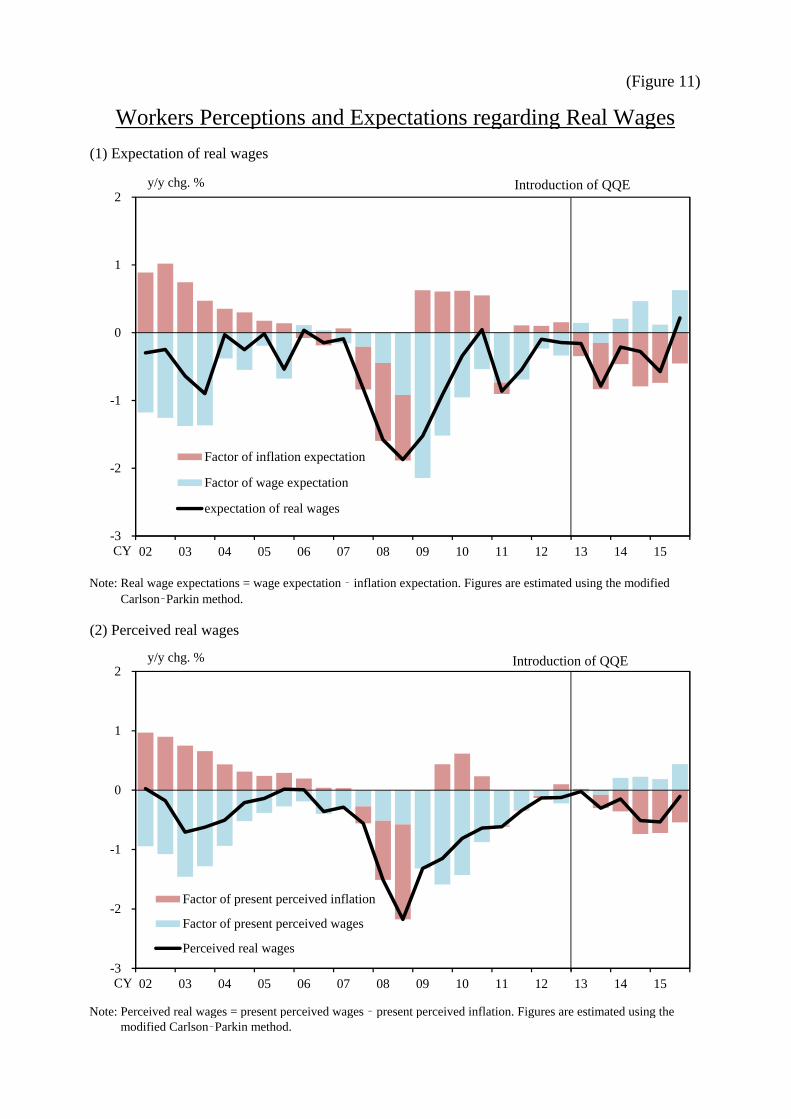
(Figure 11)

(1) Expectation of real wages

Note: Real wage expectations = wage expectation – inflation expectation. Figures are estimated using the modifiedNote: Carlson–Parkin method.

(2) Perceived real wages

Note: Perceived real wages = present perceived wages – present perceived inflation. Figures are estimated using theNote: modified Carlson–Parkin method.

Workers Perceptions and Expectations regarding Real Wages

-3

-2

-1

0

1

2

02 03 04 05 06 07 08 09 10 11 12 13 14 15

Factor of inflation expectation

Factor of wage expectation

expectation of real wages

y/y chg. %

CY

Introduction of QQE

-3

-2

-1

0

1

2

02 03 04 05 06 07 08 09 10 11 12 13 14 15

Factor of present perceived inflation

Factor of present perceived wages

Perceived real wages

y/y chg. %

CY

Introduction of QQE

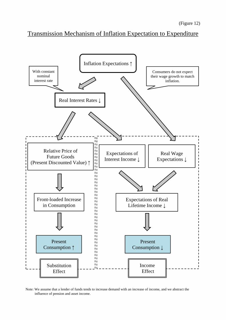
(Figure 12)

Note: We assume that a lender of funds tends to increase demand with an increase of income, and we abstract the influence of pension and asset income.

Transmission Mechanism of Inflation Expectation to Expenditure

Real Interest Rates ↓

Inflation Expectations ↑

Front-loaded Increase in Consumption

PresentConsumption ↑

Expectations of Interest Income ↓

Real Wage Expectations ↓

With constant nominal

interest rate

SubstitutionEffect

IncomeEffect

PresentConsumption ↓

Relative Price of Future Goods

(Present Discounted Value) ↑

Consumers do not expect their wage growth to match

inflation.

Expectations of Real Lifetime Income ↓

(Figure 13)

(1) Effects on real consumption

Notes: 1. Standard errors in parentheses. ***, **, * indicate significance at the 1%, 5%, and 10% levels, respectively. 2. Data for nominal rates are call rate (overnight, uncollateralized); for inflation expectation, they are the prices one year from now; for present perceived inflation, they are the prices compared with one year ago; for wage expectations, they are the wages one year from now; for present perceived wages, they are the wages compared with one year ago; and for present perceived consumption, they are the consumptions compared with one year ago.

Effects of Inflation and Wage Expectations on Consumer Spending (1)

Explanatory variables

-0.24 *** -0.22 * -0.28 *** -0.27 ** -0.23 *** -0.22 ** -0.23 ***

0.15 *** 0.15 *** 0.14 *** 0.27 *** 0.25 ***

0.47 *** 0.46 *** 0.55 *** 0.59 *** 0.65 ***

-0.03

0.12 *** 0.12 *** 0.19 ***

0.08 0.09 0.16 **

0.50 *** 0.50 *** 0.44 *** 0.31 *** 0.19 *** 0.47 *** 0.41 ***

Fixed effect of age Yes Yes Yes Yes Yes Yes Yes

Adjusted R2 0.391 0.389 0.326 0.251 0.134 0.334 0.290

Sample size 216 216 224 216 224 216 224

Spec 7

(0.08)

Real interest rate(Nominal rate ‐ Inflation

expectations)(0.08) (0.08)

Spec 1 Spec 3 Spec 4

(0.09)

Spec 5

(0.09)

Spec 6

(0.08)

Spec 2

(0.11)

Sample period: From April 2002 to October 2015

Dependent variable: Real consumption perceptions (Consumption perceptions - Inflation perceptions, year-on-year rate of changes)

Real wage perceptions(Wage perceptions ‐ Inflation

perceptions)(0.07) (0.07) (0.07)

Real wage expectations(Wage expectations ‐ Inflation

expectations)(0.04) (0.04) (0.04) (0.04)

(0.07)

Real interest rate(one-quarter lag)

Real wage perceptions(one-quarter lag) (0.07) (0.07)

Real wage expectations(one-quarter lag) (0.04) (0.04)

(0.05)Constant

(0.05) (0.05) (0.05) (0.05) (0.06)(0.06)

(0.04)

(0.08)

(0.11)

(0.04)

(0.08)

(Figure 14)

(2) Contribution to real consumption < spec 1 >

Note: Figures are calculated by accumulating the results of each groups.Sources: Cabinet Office, “National Accounts”; Ministry of Health, Labour and Welfare, “Monthly Labour Survey”;Sources: Ministry of Internal Affairs and Communications, “Consumer Price Index”;

Sources: RENGO-RIALS, “The Questionnaire Survey on Work and Life of Workers.”

Effects of Inflation and Wage Expectations on Consumer Spending (2)

03 04 05 06 07 08 09 10 11 12 13 14 15-2

-1

0

1

2Residual Factor of attribute

Constant Factor of perceived real wage

Factor of real wage expectation Factor of real interest rate

Real consumption perceptions

y/y chg. %pts

CY

Introduction of QQE

(Figure 15)

　推計結果

Notes: 1. Standard errors in parentheses. ***, **, * indicate significance at the 1%, 5%, and 10% levels, respectively.Notes: 2. In the estimation, we convert the qualitative data into the quantity data as follows: “Will rise significantly” =1, “will rise slightly” = 2, “will remain almost unchanged” = 3, “will drop slightly” = 4, and “will drop significantly” = 5.Notes: 3. The fixed effect of age is estimated using dummy variables of age group (50s, 40s, 30s, and 20s); that of employment formats is estimated using dummy variables of regular employees, part-time, so called “arbeit” workers, contract, and temps; that of the number of employees is estimated using dummy variables of less than 29, 30–99, 100–299, 300–999, and 1,000 and more employees; and that of survey date is estimated using time dummy variables.

Expectation Formation of wages (one year from now)

Explanatory variables

0.06 ** 0.04 0.01

0.58 *** 0.60 *** 0.59 ***

0.10 *** 0.11 *** 0.07 ***

0.14 *** 0.19 *** 0.16 ***

0.02

-0.04 -0.01 0.08 ***

0.24 *** 0.39 *** 0.34 ***

0.31 ***

Fixed effect of age Yes Yes Yes

Fixed effect of employment formats Yes Yes Yes

Fixed effect of the number of employees Yes Yes Yes

Fixed effect of survey date Yes Yes Yes

Threshold β1 1.03 0.79 0.61

Threshold β2 2.96 2.68 2.45

Threshold β3 5.05 4.73 4.47

Threshold β4 6.08 5.74 5.58

Pseudo R2 0.22 0.21 0.20

Estimation periods

Sample size 4,287 4,287 25,017

From Apr. 2013to Apr. 2015

From Apr. 2013to Apr. 2015

From Oct. 2005to Oct. 2015

(will increase significantly, will increase slightly, will remain almost unchanged, will decrease slightly, will decrease significantly)

Long-term outlook for economic conditions(Economic conditions three years from now) (0.03)

Spec 2

(0.03)

(0.02)

(0.03)

Long-term outlook for business performance(Business performance three years from now) (0.03)

Short-term outlook for business performance(Business performance one year from now) (0.03) (0.01)(0.03)

Perception of business performance(Business performance compared with one year ago) (0.03) (0.01)(0.03)

Short-term outlook for economic conditions(Economic conditions one year from now) (0.03) (0.01)(0.03)

Perception of economic conditions(Economic conditions compared with one year ago) (0.03) (0.01)

Wage perceptions(Wages compared with one year ago) (0.02) (0.01)

Inflation perceptions(Prices compared with one year ago) (0.03) (0.01)

Dependent variable: Wage expectations for one year from now

Spec 1 Spec 3

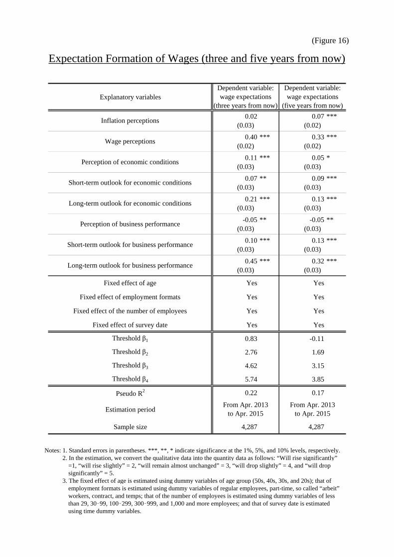
(Figure 16)

Notes: 1. Standard errors in parentheses. ***, **, * indicate significance at the 1%, 5%, and 10% levels, respectively.Notes: 2. In the estimation, we convert the qualitative data into the quantity data as follows: “Will rise significantly” =1, “will rise slightly” = 2, “will remain almost unchanged” = 3, “will drop slightly” = 4, and “will drop significantly” = 5.Notes: 3. The fixed effect of age is estimated using dummy variables of age group (50s, 40s, 30s, and 20s); that of employment formats is estimated using dummy variables of regular employees, part-time, so called “arbeit” workers, contract, and temps; that of the number of employees is estimated using dummy variables of less than 29, 30–99, 100–299, 300–999, and 1,000 and more employees; and that of survey date is estimated using time dummy variables.

Expectation Formation of Wages (three and five years from now)

Explanatory variables

0.02 0.07 ***

0.40 *** 0.33 ***

0.11 *** 0.05 *

0.07 ** 0.09 ***

0.21 *** 0.13 ***

-0.05 ** -0.05 **

0.10 *** 0.13 ***

0.45 *** 0.32 ***

Fixed effect of age Yes Yes

Fixed effect of employment formats Yes Yes

Fixed effect of the number of employees Yes Yes

Fixed effect of survey date Yes Yes

Threshold β1 0.83 -0.11

Threshold β2 2.76 1.69

Threshold β3 4.62 3.15

Threshold β4 5.74 3.85

Pseudo R2 0.22 0.17

Estimation period

Sample size 4,287 4,287

Perception of business performance(0.03) (0.03)

From Apr. 2013to Apr. 2015

From Apr. 2013to Apr. 2015

Short-term outlook for business performance(0.03) (0.03)

Long-term outlook for business performance(0.03) (0.03)

Short-term outlook for economic conditions(0.03) (0.03)

Long-term outlook for economic conditions(0.03) (0.03)

Wage perceptions(0.02) (0.02)

Perception of economic conditions(0.03) (0.03)

Dependent variable:wage expectations

(three years from now)

Dependent variable:wage expectations

(five years from now)

Inflation perceptions(0.03) (0.02)

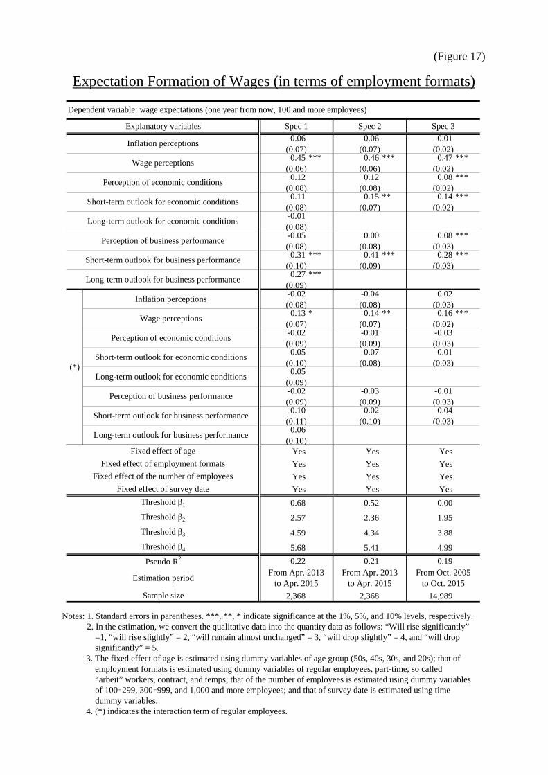
(Figure 17)

Notes: 1. Standard errors in parentheses. ***, **, * indicate significance at the 1%, 5%, and 10% levels, respectively.Notes: 2. In the estimation, we convert the qualitative data into the quantity data as follows: “Will rise significantly” =1, “will rise slightly” = 2, “will remain almost unchanged” = 3, “will drop slightly” = 4, and “will drop significantly” = 5. 3. The fixed effect of age is estimated using dummy variables of age group (50s, 40s, 30s, and 20s); that of employment formats is estimated using dummy variables of regular employees, part-time, so called “arbeit” workers, contract, and temps; that of the number of employees is estimated using dummy variables of 100–299, 300–999, and 1,000 and more employees; and that of survey date is estimated using time dummy variables. 4. (*) indicates the interaction term of regular employees.

Expectation Formation of Wages (in terms of employment formats)

0.06 0.06 -0.01

0.45 *** 0.46 *** 0.47 ***

0.12 0.12 0.08 ***

0.11 0.15 ** 0.14 ***

-0.01

-0.05 0.00 0.08 ***

0.31 *** 0.41 *** 0.28 ***

0.27 ***

-0.02 -0.04 0.02

0.13 * 0.14 ** 0.16 ***

-0.02 -0.01 -0.03

0.05 0.07 0.01

0.05

-0.02 -0.03 -0.01

-0.10 -0.02 0.04

0.06

Yes Yes Yes

Yes Yes Yes

Yes Yes Yes

Yes Yes Yes

0.68 0.52 0.00

2.57 2.36 1.95

4.59 4.34 3.88

5.68 5.41 4.99

0.22 0.21 0.19

2,368 2,368 14,989Sample size

Fixed effect of age

Fixed effect of employment formats

Fixed effect of the number of employees

Fixed effect of survey date

Threshold β2

Threshold β3

Threshold β4

Pseudo R2

Estimation period

(*)

Threshold β1

Inflation perceptions

Wage perceptions

Perception of economic conditions

Short-term outlook for economic conditions

Long-term outlook for economic conditions

Perception of business performance

Short-term outlook for business performance

Long-term outlook for business performance

Short-term outlook for business performance

Long-term outlook for business performance

Long-term outlook for economic conditions

Perception of economic conditions

Inflation perceptions

(0.10) (0.09) (0.03)

(0.09)

(0.08)

(0.08) (0.08) (0.03)

(0.02)

(0.08) (0.08) (0.02)

(0.08) (0.07) (0.02)

From Apr. 2013to Apr. 2015

From Apr. 2013to Apr. 2015

From Oct. 2005to Oct. 2015

(0.07) (0.07) (0.02)

(0.06) (0.06)

(0.11) (0.10) (0.03)

(0.10)

(0.09)

Perception of business performance(0.09) (0.09) (0.03)

(0.09) (0.09) (0.03)

Short-term outlook for economic conditions(0.10) (0.08) (0.03)

(0.08) (0.08) (0.03)

Wage perceptions(0.07) (0.07) (0.02)

Spec 1 Spec 2 Spec 3

Dependent variable: wage expectations (one year from now, 100 and more employees)

Explanatory variables

(Figure 18)

Notes: 1. Standard errors in parentheses. ***, **, * indicate significance at the 1%, 5%, and 10% levels, respectively.Notes: 2. In the estimation, we convert the qualitative data into the quantity data as follows: “Will rise significantly” =1, “will rise slightly” = 2, “will remain almost unchanged” = 3, “will drop slightly” = 4, and “will drop significantly” = 5. 3. The fixed effect of age is estimated using dummy variables of age group (50s, 40s, 30s, and 20s); that of the number of employees is estimated using dummy variables of 100–299, 300–999, and 1,000 and more employees; and that of survey date is estimated using time dummy variables. 4. (*) indicates the interaction term of a regular employees whose workplace has a labor union.

Expectation Formation of Wages (in terms of presence of labor unions)

0.07 0.04 0.02

0.57 *** 0.59 *** 0.63 ***

0.19 *** 0.20 *** 0.05 **

0.13 ** 0.21 *** 0.14 ***

0.06

-0.19 *** -0.15 *** 0.04

0.28 *** 0.42 *** 0.35 ***

0.29 ***

-0.04 -0.04 -0.01

0.00 -0.01 0.01

-0.13 -0.13 -0.01

0.03 0.00 0.02

-0.08

0.25 *** 0.24 *** 0.06 *

-0.13 -0.07 -0.06 *

0.09

Yes Yes YesYes Yes YesYes Yes Yes0.94 0.75 0.29

2.92 2.69 2.39

4.89 4.62 4.24

5.97 5.66 5.41

0.23 0.21 0.21

1,738 1,738 10,716

Threshold β1

From Oct. 2005to Oct. 2015

Sample size

Threshold β3

Threshold β4

Pseudo R2

Estimation periodFrom Apr. 2013

to Apr. 2015From Apr. 2013

to Apr. 2015

Wage perceptions(0.07)

Fixed effect of ageFixed effect of the number of employees

Fixed effect of survey date

Perception of business performance(0.08) (0.08) (0.03)

Threshold β2

Short-term outlook for business performance(0.10) (0.09) (0.03)

Long-term outlook for business performance(0.10)

(*)

Inflation perceptions(0.06)

Short-term outlook for economic conditions(0.10) (0.08) (0.03)

Long-term outlook for economic conditions(0.09)

(0.07) (0.03)

Perception of economic conditions

Short-term outlook for business performance(0.06) (0.06) (0.03)

Long-term outlook for business performance(0.06)

(0.09) (0.09) (0.03)

(0.06) (0.02)

Long-term outlook for economic conditions(0.06)

Perception of business performance(0.06) (0.06) (0.02)

Perception of economic conditions(0.06) (0.06) (0.02)

Short-term outlook for economic conditions(0.06) (0.05) (0.02)

Inflation perceptions(0.05) (0.05) (0.02)

Wage perceptions(0.05) (0.05) (0.02)

Dependent variable: wage expectation (one year from now, regular employees, 100 and more employees)

Explanatory variables Spec 1 Spec 2 Spec 3

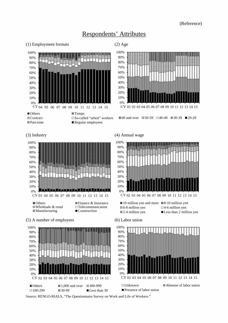
(Reference)

(1) Employment formats (2) Age

(3) Industry (4) Annual wage

(5) A number of employees (6) Labor union

Source: RENGO-RIALS, “The Questionnaire Survey on Work and Life of Workers.”

Respondents’ Attributes

0%

10%20%30%40%

50%60%70%80%90%

100%

04 05 06 07 08 09 10 11 12 13 14 15

Others TempsContract So-called “arbeit” workersPart-time Regular employees

CY

0%10%20%30%40%50%60%70%80%90%

100%

03 04 05 06 07 08 09 10 11 12 13 14 15

Others Finance & InsuranceWholesale & retail TelecommunicationManufacturing Construction

CY0%

10%20%30%40%50%60%70%80%90%

100%

02 03 04 05 06 07 08 09 10 11 12 13 14 15

10 million yen and more 8-10 million yen6-8 million yen 4-6 million yen2-4 million yen Less than 2 million yen

CY

0%10%20%30%40%50%60%70%80%90%

100%

02 03 04 05 06 07 08 09 10 11 12 13 14 15

Others 1,000 and over 300-999100-299 30-99 Less than 30

CY

0%

10%

20%

30%40%

50%

60%

70%

80%90%

100%

01 02 03 04 05 06 07 08 09 10 11 12 13 14 15

60 and over 50-59 40-49 30-39 20-29

CY

0%10%20%30%40%50%60%70%80%90%

100%

02 03 04 05 06 07 08 09 10 11 12 13 14 15

Unknown Absense of labor unionPresence of labor union

CY