Embed Size (px)
Citation preview
The Impact of Peer Ability and Heterogeneity on Student Achievement:
Evidence from a Natural Experiment
David Kiss, April 02, 2011
Abstract:
This paper estimates the impact of peer achievement and variance on math achievement
growth. It exploits exogenous variation in peer characteristics generated at the transition to
upper-secondary school in a sample of Berlin fifth-graders. Parents and schools are barely
able to condition their decisions on peer characteristics since classes are newly built up from a
large pool of elementary school pupils. I find positive peer effects on achievement growth and
no effects for peer variance. Lower-achieving pupils benefit more from abler peers. Results
from simulations suggest that pupils are slightly better off in comprehensive than in ability-
tracked school systems. JEL: I21, I28.
Keywords: peer effects in secondary school, comparison between ability-tracked and compre-
hensive school, natural experiment
University of Erlangen-Nuremberg, Lange Gasse 20, D-90403 Nuremberg, Germany, [email protected]. I
wish to thank Regina T. Riphahn, Christoph Wunder, and Michael Zibrowius for valuable comments and suggestions. Help-
ful insights by participants of the BGPE Research Workshop (Passau) are gratefully acknowledged. The data (ELEMENT)
were produced by the Humboldt University of Berlin and provided to me by the research data center (FDZ) at IQB Berlin,
whose staff I thank for their help and support. All remaining errors are mine.
1
1. Introduction
Peer group composition of classes plays an essential role for school choice decisions of par-
ents. Peer effects are also important in debates on school vouchers, desegregation, ability
tracking or antipoverty programs. This paper investigates the (causal) impact of peer ability
and heterogeneity on student achievement in math. It exploits exogenous variation in peer
group characteristics which is generated in newly built up classes at the transition of Berlin
students to upper-secondary school after the fourth grade.
All studies about peer ability and its impact on achievement growth are aware of the
existence of severe endogeneity problems. Peer characteristics and student achievement are
spuriously correlated if, for instance, children of ambitious parents (i) are more likely to be
placed into classes with high-achieving and homogenous peers, and (ii) generally get more
support, like private tuition. School principals could also tend to group pupils into classes
strategically, particularly if school accountability systems are implemented.1
There are two bodies of convincing research that investigate the impact of peer ability
on achievement growth: the first extensively makes use of fixed-effects frameworks whereas
the second aims to exploit exogenous variation generated in (quasi-) experimental settings.
Both have in common the estimation of models of educational production that account at least
for lagged student and peer achievement. These two variables are assumed to capture past
family, peer, and school inputs.2 Specifications based on cross-sectional data cannot account
for past achievement. This yields biased estimates for the impact of peer ability on student
achievement because of simultaneity: if peers have an influence on a student's achievement,
that student will also affect his/her peers' achievement.3
1 There is evidence for the existence of school gaming behavior under accountability pressure: threatened schools may reclas-
sify low-achieving students into special education, see Figlio and Getzler (2002). As shown in Jacob and Levitt (2003), some
of them even manipulate testing conditions by teacher cheating. 2 Summers and Wolfe (1977) are one of the first who estimate such models of educational production. Using data of sixth-
graders from the Philadelphia School District, they find positive peer effects on (composite) student achievement. 3 This problem is also referred to as the "reflection problem", see Manski (1993).

2
Hanushek et al. (2003) and Sund (2009) belong to the first strand of research.
Hanushek et al. (2003) analyze a large data set of Texas public elementary school pupils
(grades three through six). Controlling for fixed student, school, and school-by-grade effects
and an additional number of time-varying student, family, and school characteristics, their
results suggest that peer heterogeneity has no significant impact on math learning. Further, a
standard deviation increase in peer achievement is associated with a 0.2 increase in (standard-
ized) math achievement, which is substantial. Accounting for time, school, teacher, and indi-
vidual fixed effects, Sund (2009) also finds positive peer effects among Swedish students who
are enrolled in upper-secondary school.4 Surprisingly, students are better off in classes that are
more heterogeneous. He additionally shows that lower-achieving students benefit more from
an increase in peer ability than their higher-achieving classmates.
Alternatively, the second strand of research exploits situations where students are
(quasi-) randomly grouped into classes. Form the viewpoint of an ideal experiment, random
grouping of pupils could reveal the causal impact of peer achievement and peer heterogeneity
on achievement growth since variation in peer characteristics is exogenous in this setting.5
Such an event is analyzed in Carrell, Fullerton, and West (2009), where U.S. Air Force Acad-
emy freshmen are exogenously assigned to peer groups of approximately 30 students. In the
first year of their university study, these students have limited ability to interact with other
students outside of their assigned peer group. Thus these groups might be considered as clas-
ses. The authors find positive peer effects in math and science courses. No results are reported
for the impact of peer heterogeneity on achievement growth.6
Results presented in this study are obtained from a natural experiment in Berlin upper-
secondary schools. Each school year, classes at the fifth grade are newly built up with pupils
4 In Sweden, compulsory education is comprehensive and lasts for nine years. Subsequently, pupils have the possibility to
attend upper-secondary school. 5 Research designs that seek to mimic such situations are strongly advocated by Angrist and Pischke (2010). 6 Using the same identification strategy, Sacerdote (2001) reports similar results for the impact of peer effects on freshmen
GPA (Grade Point Average).
3
from a large number of elementary schools. This situation is similar to Carrell, Fullerton, and
West (2009), where peer groups are built up from the pool of Air Force Academy freshmen.
The identification strategy, which will be outlined in more detail, depends on two assump-
tions: (i) parents of fourth-graders are not able to condition their school choice decision on
peer characteristics because classes at the fifth grade are built up in the future. (ii) Upper-
secondary schools have limited possibilities to group fifth-graders by skill at the beginning of
a school year – to do so, schools need to monitor pupils for a time.
This study further analyses which students are better off in ability-tracked and com-
prehensive school systems. Some countries, e.g. Germany or the Netherlands, group students
by ability into different secondary school tracks at ages between 10 and 12. By contrast, the
lower-secondary school systems of Japan, Norway, the UK, and the US are comprehensive
and do not track at all.
The analysis of the data suggests that pupils benefit from an increase in peer math
achievement but higher-achieving students do so to a smaller extent. Peer heterogeneity, as
measured by peer variance and alternative measures of dispersion, seems not to affect math
achievement growth. The results also indicate that pupils with high class percentile ranks
(high-achievers within classes) learn more. Depending on the estimates, simulations show that
slightly more than the majority of pupils are better off in comprehensive than ability-tracked
school systems. The simulations also suggest that the degree of homogeneity and mean
achievement of the student body becomes somewhat higher in comprehensive school. The
major shortcoming of this study is related to the external validity of the results because they
are obtained from a sample of upper-secondary pupils. They might not be representative for
the whole student body which could result, for instance, in biased simulation results.
The remainder of the paper is as follows: section 2 briefly describes the data. The
identification strategy is outlined in section 3. Section 4 presents the main results. Using

4
simulated data, the winners and losers from a school system change towards comprehensive
school are described in section 5. Section 6 concludes.
2. Data and summary statistics
In Germany, elementary school generally lasts until the fourth grade when children are 10
years old. Thereafter students are tracked by ability into three types of secondary schools:
lower-secondary (Hauptschule), middle-secondary (Realschule), and upper-secondary school
(Gymnasium). Upper-secondary school is the most academic track and prepares students for
university study. The Berlin educational system is somewhat different since primary educa-
tion lasts six years. Some Berlin upper-secondary schools, however, allow transition after four
years of elementary school.7 In the following, these upper-secondary schools are referred to as
G5 schools. In the school year 2002/03 around 24,200 fourth-graders attended one of 402
Berlin elementary schools. 7% of them changed to one of 31 G5 schools in the following
school year.8
The data analyzed here is called ELEMENT.9 It is a longitudinal survey on reading
comprehension and math achievement of Berlin elementary and G5 pupils. In the primary
school sample, classes at the fourth grade (primary sampling units) were randomly drawn in
the school year 2002/03. To allow within-school comparisons, a second class from the same
school was additionally drawn if possible. The primary school sample contains 13% of all
elementary school fourth-graders (71 schools, 140 classes, 3293 pupils). This cohort of
fourth-graders was followed through grades four to six. Further, all fifth-graders that attended
a G5 school in the school year 2003/04 were included and followed through grades five to six
(31 schools, 59 classes, 1700 pupils).
7 In contrast, transition into lower- or middle-secondary schools is not possible after the fourth grade. 8 At that time, the number of Berlin upper-secondary schools (including G5 schools) was 111. 9 "Erhebung zum Lese- und Mathematikverständnis: Entwicklungen in den Jahrgangsstufen 4 bis 6 in Berlin", English trans-
lation: "Survey on reading comprehension and math achievement in Berlin schools, grades 4 through 6". Detailed data de-
scriptions and a codebook (both in German) are available on the homepages of the Berlin senate department for education,
science, and research (Berliner Senatsverwaltung für Bildung, Wissenschaft und Forschung).
5
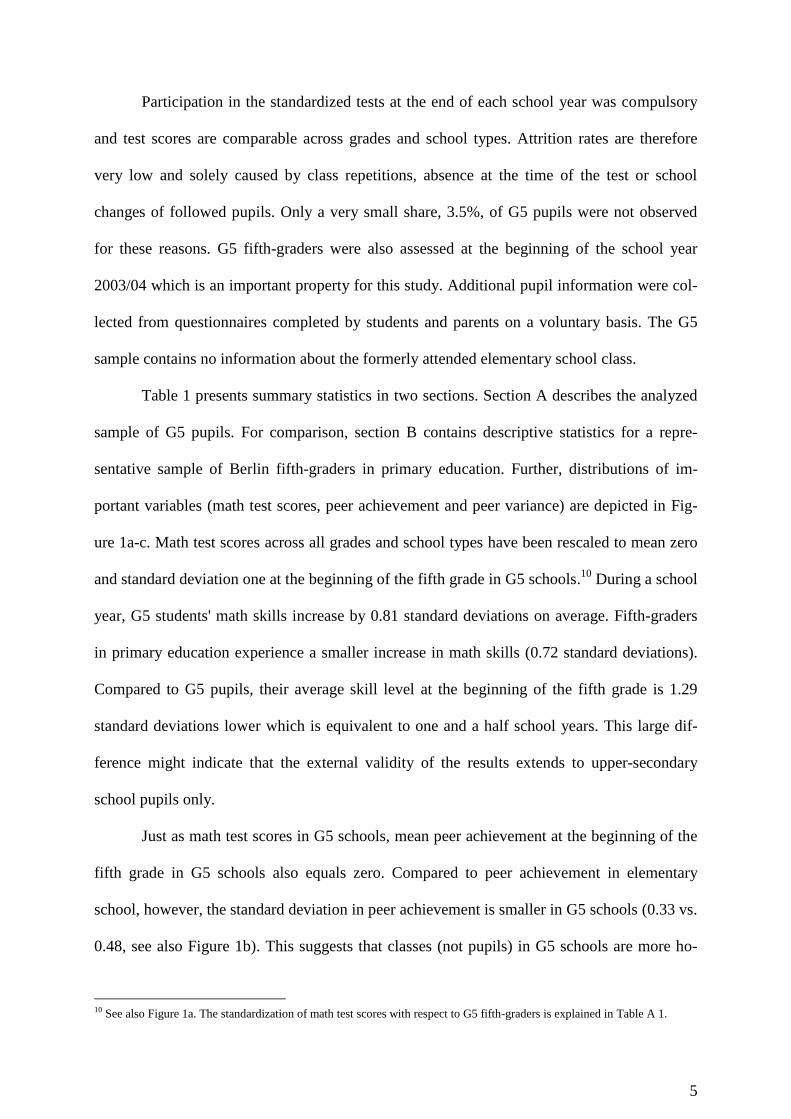
Participation in the standardized tests at the end of each school year was compulsory
and test scores are comparable across grades and school types. Attrition rates are therefore
very low and solely caused by class repetitions, absence at the time of the test or school
changes of followed pupils. Only a very small share, 3.5%, of G5 pupils were not observed
for these reasons. G5 fifth-graders were also assessed at the beginning of the school year
2003/04 which is an important property for this study. Additional pupil information were col-
lected from questionnaires completed by students and parents on a voluntary basis. The G5
sample contains no information about the formerly attended elementary school class.
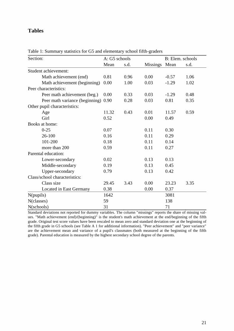
Table 1 presents summary statistics in two sections. Section A describes the analyzed
sample of G5 pupils. For comparison, section B contains descriptive statistics for a repre-
sentative sample of Berlin fifth-graders in primary education. Further, distributions of im-
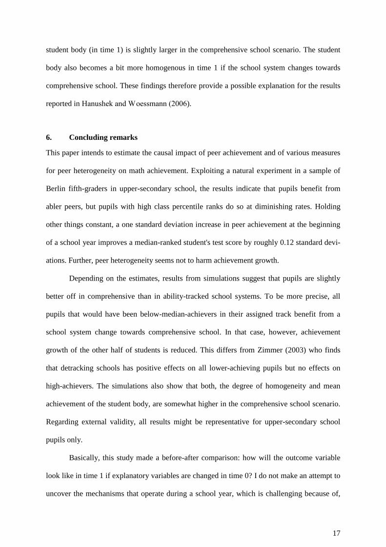
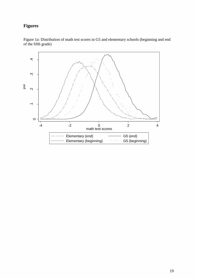
portant variables (math test scores, peer achievement and peer variance) are depicted in Fig-
ure 1a-c. Math test scores across all grades and school types have been rescaled to mean zero
and standard deviation one at the beginning of the fifth grade in G5 schools.10
During a school
year, G5 students' math skills increase by 0.81 standard deviations on average. Fifth-graders
in primary education experience a smaller increase in math skills (0.72 standard deviations).
Compared to G5 pupils, their average skill level at the beginning of the fifth grade is 1.29
standard deviations lower which is equivalent to one and a half school years. This large dif-
ference might indicate that the external validity of the results extends to upper-secondary
school pupils only.
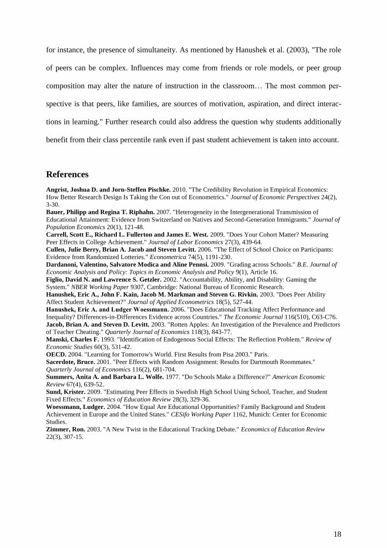
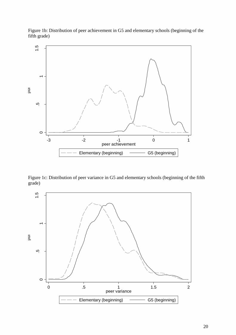
Just as math test scores in G5 schools, mean peer achievement at the beginning of the
fifth grade in G5 schools also equals zero. Compared to peer achievement in elementary
school, however, the standard deviation in peer achievement is smaller in G5 schools (0.33 vs.
0.48, see also Figure 1b). This suggests that classes (not pupils) in G5 schools are more ho-
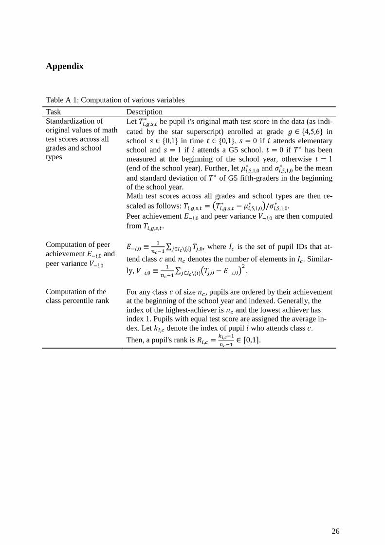
10 See also Figure 1a. The standardization of math test scores with respect to G5 fifth-graders is explained in Table A 1.
6
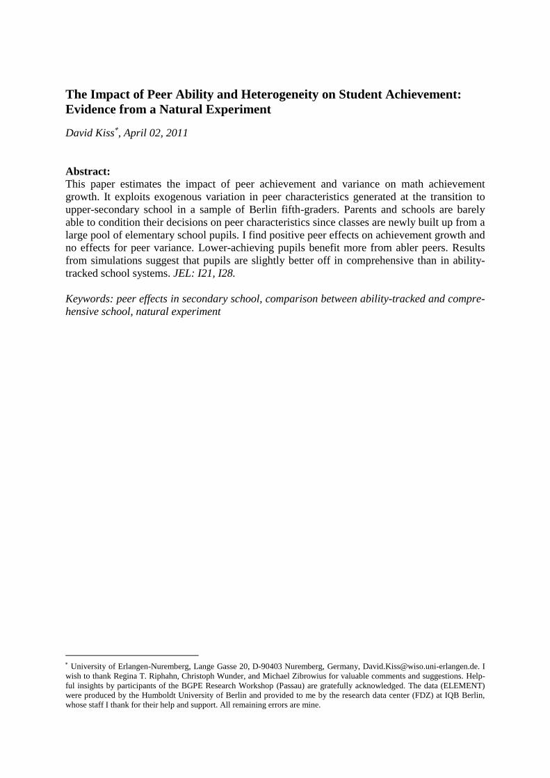
mogenous in terms of mean class achievement. Students who attend same classes, however,
are more heterogeneous in G5 schools. As the summary statistics for mean peer variance
show, the degree of within-class heterogeneity is somewhat larger in G5 schools (0.90 vs.
0.81, see also Figure 1c). This indicates that G5 schools might not primarily seek to build up
classes that are homogenous in math skills.11
Most G5 pupils have a favorable socioeconomic
background: 80% of their parents finished upper-secondary school and have at least 100
books at home.12
This could account for the large difference in mean achievement between
G5 and elementary school fifth-graders.13
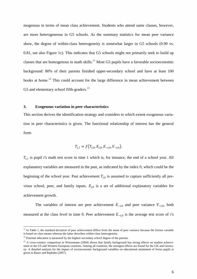
3. Exogenous variation in peer characteristics
This section derives the identification strategy and considers to which extent exogenous varia-
tion in peer characteristics is given. The functional relationship of interest has the general
form
( ).
is pupil 's math test score in time 1 which is, for instance, the end of a school year. All
explanatory variables are measured in the past, as indicated by the index 0, which could be the
beginning of the school year. Past achievement is assumed to capture sufficiently all pre-
vious school, peer, and family inputs. is a set of additional explanatory variables for
achievement growth.
The variables of interest are peer achievement and peer variance , both
measured at the class level in time 0. Peer achievement is the average test score of 's
11 In Table 1, the standard deviation of peer achievement differs from the mean of peer variance because the former variable
is based on class means whereas the latter describes within-class heterogeneity. 12 Parental education is measured by the highest secondary school degree of the parents. 13 A cross-country comparison in Woessmann (2004) shows that family background has strong effects on student achieve-
ment in the US and Western European countries. Among all countries, the strongest effects are found for the UK and Germa-
ny. A detailed analysis for the impact of socioeconomic background variables on educational attainment of Swiss pupils is
given in Bauer and Riphahn (2007).

7
classmates. The calculation of this average excludes as emphasized by the subscript .
Computing in this manner rules out the possibility that any correlation between and
is caused by .14
Peer variance is calculated in a similar way.15
The experiment that could ideally be used to capture the causal effect of peer
achievement and peer heterogeneity on student achievement would be random grouping of
pupils into classes. Pupils who enter a G5 school after four years of primary education are in a
similar situation since parents and schools have limited capabilities to condition their school-
choice decisions on peer ability and heterogeneity and G5 schools might also not be interested
in doing so.
In primary education, the mean and variance of peer achievement could be endoge-
nous for several reasons. If ambitious parents systematically keep their child away from at-
tending classes or schools with underperforming or very heterogeneous peers, and if they are
more likely to support the educational progress of their child (e.g. homework assistance, pri-
vate tuition), then achievement growth and peer characteristics might be correlated. Endoge-
neity caused by omitted variables could also arise in elementary schools if certain school
principals are interested in raising mean achievement by ability-grouping of pupils into clas-
ses. To do so, however, parents and school principals need to monitor pupils for a certain
time.
These problems do not arise or can be accounted for in G5 schools at the beginning of
the fifth grade. Parents have to apply for a G5 school six months in advance of which implies
that they cannot condition their application (and registration) at least on peer heterogeneity of
the future G5 class. However, parents can expect that peer achievement in math is higher in
14 To make this point clear, let be the mean achievement in 's class (including 's own test score) which implies
if two (different) pupils and attend the same class. Further, let be the correlation coefficient between two variables
and . Obviously, ( ) . If ( ) is also true, then and must be positively correlated. 15 The computation of peer achievement and variance is explained in more detail in Table A 1.
8
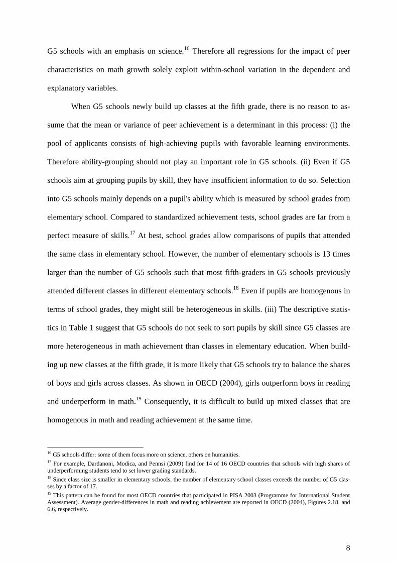
G5 schools with an emphasis on science.16
Therefore all regressions for the impact of peer
characteristics on math growth solely exploit within-school variation in the dependent and
explanatory variables.
When G5 schools newly build up classes at the fifth grade, there is no reason to as-
sume that the mean or variance of peer achievement is a determinant in this process: (i) the
pool of applicants consists of high-achieving pupils with favorable learning environments.
Therefore ability-grouping should not play an important role in G5 schools. (ii) Even if G5
schools aim at grouping pupils by skill, they have insufficient information to do so. Selection
into G5 schools mainly depends on a pupil's ability which is measured by school grades from
elementary school. Compared to standardized achievement tests, school grades are far from a
perfect measure of skills.17
At best, school grades allow comparisons of pupils that attended
the same class in elementary school. However, the number of elementary schools is 13 times
larger than the number of G5 schools such that most fifth-graders in G5 schools previously
attended different classes in different elementary schools.18
Even if pupils are homogenous in
terms of school grades, they might still be heterogeneous in skills. (iii) The descriptive statis-
tics in Table 1 suggest that G5 schools do not seek to sort pupils by skill since G5 classes are
more heterogeneous in math achievement than classes in elementary education. When build-
ing up new classes at the fifth grade, it is more likely that G5 schools try to balance the shares
of boys and girls across classes. As shown in OECD (2004), girls outperform boys in reading
and underperform in math.19
Consequently, it is difficult to build up mixed classes that are
homogenous in math and reading achievement at the same time.
16 G5 schools differ: some of them focus more on science, others on humanities. 17 For example, Dardanoni, Modica, and Pennsi (2009) find for 14 of 16 OECD countries that schools with high shares of
underperforming students tend to set lower grading standards. 18 Since class size is smaller in elementary schools, the number of elementary school classes exceeds the number of G5 clas-
ses by a factor of 17. 19 This pattern can be found for most OECD countries that participated in PISA 2003 (Programme for International Student
Assessment). Average gender-differences in math and reading achievement are reported in OECD (2004), Figures 2.18. and
6.6, respectively.
9
This reasoning motivates the identification strategy: within-school variation in the
mean and variance of peer achievement is assumed to be exogenous and estimates of their
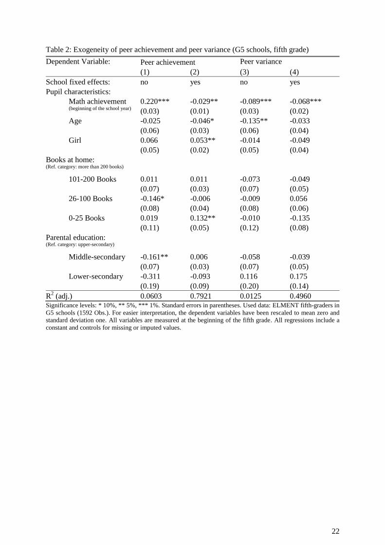
coefficients may be interpreted causally. To test the exogeneity of peer achievement and vari-
ance at the fifth grade in G5 schools, these two variables are regressed on math achievement
and other explanatory variables in Table 2. All variables are measured at the beginning of the
school year. For easier interpretation, the dependent variables have been rescaled to mean
zero and standard deviation one. Columns 1 and 3 do not account for school fixed effects –
these are controlled for in columns 2 and 4.
In the case of perfect randomization, one would expect insignificant estimates with ab-
solute values close to zero. One can infer from Table 2, column 1 that higher-achieving stu-
dents are more likely to have abler peers. The point estimate is large and highly significant.
Thus results from regressions that exclude school fixed effects might be biased because of
self-selection of high-achievers into classes with abler peers. As already mentioned, mean
math achievement could be higher in G5 schools that put an emphasis on science and lower in
G5 schools focusing more on humanities. The results from column 2 seem to confirm this
hypothesis: once school fixed effects are accounted for, the point estimate for math achieve-
ment remains significant, but turns negative with an absolute value close to zero. Similarly,
peer variance and student achievement are correlated, but point estimates in columns 3 and 4
are also close to zero.
Regarding the remaining explanatory variables, there seems to be no systematic self-
selection into classes or schools with specific levels of peer achievement or variance since
most related coefficients are either insignificant or close to zero. Further, the few significant
estimates are not robust since they are sensitive to the in- or exclusion of school fixed effects.
Summing up, endogeneity cannot be ruled out completely, but is likely to play a minor role
once school fixed effects are taken into account.
10
4. Results
The impact of peer characteristics on achievement growth is estimated with the following
baseline-model of educational production:
is pupil 's math test score at the end of the fifth grade as indicated by the subscript 1. All
variables on the RHS are indexed with 0 which stands for "beginning of fifth grade". The ex-
planatory variables are therefore predetermined which rules out simultaneity. Peer achieve-
ment is the average test score of 's classmates at the beginning of the fifth grade. By
assumption, sufficiently captures past school and family inputs of the peers. Since G5
classes are built up from a large pool of elementary school fourth-graders, the probability is
small that pupils who are grouped into a G5 class previously attended the same elementary
school classes. Therefore should not be biased because of peer-interactions in the past.
is the variance of 's peers.
is pupil 's class percentile rank in math test scores. By definition, .
Within classes, the highest-achieving pupil has rank one, the median-achiever has rank 0.5
and the lowest-achiever has been assigned rank zero. , the math test score at the beginning
of the fifth grade, is the most important control variable. It captures 's past educational inputs
and additionally accounts for the correlation between and .20
is a column-vector
which contains a constant and a set of additional controls, namely: age, a girl dummy, and the
highest educational background of parents. is a school fixed effect. Disturbances allow
for correlated residuals among students that attend same G5 classes.
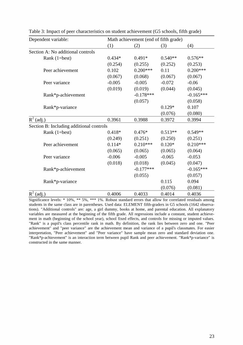
Table 3 reports estimates for the impact of peer characteristics on math achievement
growth in G5 schools. It is divided into a top and a bottom section. Section A excludes addi-
20 Pupils with high test scores are likely to have a high rank. If past achievement is left out in a regression of present
achievement on past rank , then past rank would pick up the correlation between past and present achievement. On the
other hand, two pupils with same test score may have different ranks if they attend different classes.
11
tional controls – these are taken into account in section B. Across all specifications (col-
umns 1-4) the results are not sensitive to the inclusion of but become somewhat more pre-
cise. For easier interpretation, peer achievement and peer variance have sample mean zero and
standard deviation one.
Estimates in column 1 suggest that higher ranked pupils learn more during a school
year.21
This is consistent with Cullen, Jacob, and Levitt (2006), who also find that a student's
relative position among his/her peers is an important determinant of his/her success in school.
The point estimate for peer variance is close to zero and insignificant. The impact of peer
achievement is positive and significant in section B only, the significance test yields a p-value
of 0.13 in section A.
In both sections, the effect of peer achievement is estimated with low precision since
highly ranked pupils benefit less from an increase in peer achievement (column 2). Based on
the estimates in section B, column 2, the total derivative with respect to peer achievement and
class percentile rank is:
( ) ( )
The first term indicates that students benefit from a rank increase, however, the effect
is smaller in classes with high peer achievement.22
Regarding the second term, all pupils ben-
efit from an increase in peer achievement since , but highly ranked pupils do so to
a smaller extent.23
One common explanation for this pattern is that low-ability students might
learn from better-achieving peers during a school year. Since highly ranked pupils do not have
this advantage, their returns to an increase in peer achievement decline. Further, one can infer
from these findings that placing an (average) pupil into a class with low peer achievement is
not necessarily harmful: on the one hand, that pupil's educational progress is lowered by
21 All regressions in Table 3 and Table 4 control for student achievement at the beginning of the fifth grade. 22 The effect in the first term becomes negative if , which is extremely high. 23 This relation is also found in Sund (2009) and Zimmer (2003).
12
his/her peers, on the other, that pupil is likely to benefit from an increase in his/her percentile
rank.
The third column in Table 3 checks whether pupils also respond differently to changes
in peer variance. Similar to the previous specifications (columns 1-2), peer variance does not
harm G5 fifth-graders. The fully interacted model (column 4) confirms the findings from the
second specification: pupils benefit from an increase in peer achievement or their rank and
peer variance is irrelevant. These patterns (significance levels, relations among estimates)
remain the same if controls for missing or imputed values are left out from the regressions,
but absolute values of the estimates become about 10% larger in that case.
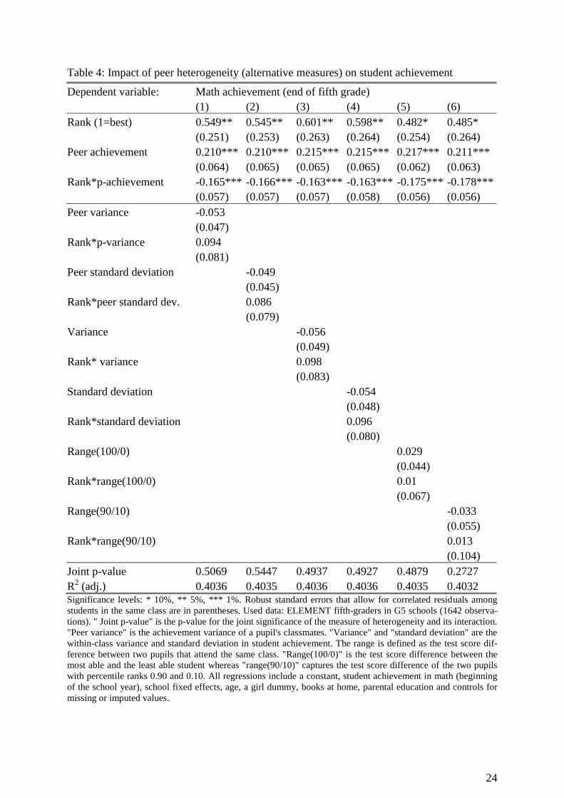
So far, the results show that peer heterogeneity does not harm student achievement. To
test this finding, Table 4 reports results for alternative measures for heterogeneity. Column 1
controls for peer variance. These estimates are therefore identical with the fourth column in
Table 3, section B. In the second column of Table 4, peer standard deviation instead of peer
variance is used to measure heterogeneity. The additional alternative measures (columns 3-6)
are constant among pupils that attend the same classes – these measures therefore only vary
across classes. Columns 3 and 4 report results for the "common" variance and standard devia-
tion (including pupil ), respectively. Columns 5 and 6 show results for two measures for the
range. The range is defined as the test score difference between two pupils that attend the
same class. Range(100/0) is the test score difference between the most able and the least able
student whereas range(90/10) captures the test score difference of the two pupils with percen-
tile ranks 0.90 and 0.10.
All estimates for the impact of peer heterogeneity and the interaction between rank
and peer heterogeneity are (jointly) insignificant in Table 4 and the main findings from Table
3 are confirmed. The results in Table 4 are virtually unaffected by the in- or exclusion of addi-
tional controls and control variables for missing or imputed values. If peer achievement and
13
various measures for peer heterogeneity are not interacted with the percentile rank, the results
become very similar to the findings reported in Table 3, column 1.
5. Are pupils better off in a comprehensive or ability-tracked school system?
This section aims to identify which groups of pupils are better off in ability-tracked compared
to comprehensive school systems. Ability-tracking implies that the heterogeneity in student
achievement within tracks is smaller than the heterogeneity of the whole student body. Fur-
ther, mean achievement of students enrolled in the highest-level track should exceed mean
achievement in the lower-level tracks. Compared to ability-tracking, classes in comprehensive
schools are similar in terms of mean achievement and tend to be more heterogeneous.
Hanushek and W oessmann ( ) provide empirical evidence that the heterogeneity of the
student body increases in countries with tracked school systems. They also find that early
tracking might reduce mean performance.
Simulations allow us to identify students that would benefit and suffer from a school-
system change from ability-tracking towards comprehensive school. Using the estimates from
the previous section, one can predict and compare each student's achievement in both school
systems. The setup of the simulation implemented here is simple: there are two points in time,
beginning and end of the school year which are referred to as time 0 and time 1. In time 0, a
pupil's initial ability is drawn from the standard normal distribution. These pupils are then
either grouped by ability into three different tracks or randomly placed into classes.24
For both
scenarios (tracked or comprehensive school), the rank and peer achievement are computed for
time 0. In time 0, the expected value of mean achievement in the middle track equals the ex-
pected value of mean achievement in any comprehensive school class. Using the estimates in
Table 3 (column 2, section B), each pupil's potential achievement growth in both school sys-
24 Without any loss in generality, the simulated data used here solely consists of 90 pupils that are grouped (by ability or
randomly) into three classes of size 30. The number of replications is 10,000 which ensures the robustness of the results. For
each replication, the random-number seed is set to the current value of the replication counter.
14
tems is predicted.25
Predictions solely depend on the rank, peer achievement and the interac-
tion between rank and peer achievement.
The winners and losers from a school system change towards comprehensive school
are described in Table 5. In columns 1 and 2, pupils are assigned to six groups (column 1)
depending on their initial achievement in time 0. Initial achievement is drawn from the stand-
ard normal distribution. Pupils are then ordered by their percentile in the achievement distri-
bution (column 2). For instance, all pupils in group 1 and 2 belong to the bottom third of the
achievement distribution.26
Columns 3 to 5 contain information about each group's situation in a scenario of per-
fect ability-tracking. One can infer from column 3, that all pupils from group 1 and 2 would
have attended lower-secondary school, and all pupils from the top third of the achievement
distribution (groups 5 and 6) would be enrolled in upper-secondary education. In an ability-
tracked system, peer achievement is heterogeneous among secondary school types (column
4). For example, average-achievers (groups 3 and 4) are expected to attend middle-secondary
school where peer achievement is expected to be zero which is the median of the standard
normal distribution. Consequently, peer achievement in lower-secondary or upper-secondary
school is expected to be smaller or greater than zero, respectively. Regarding their ranks, pu-
pils from groups 2, 4, and 6 are expected to have high ranks within their assigned secondary
school track (column 5).27
For instance, pupils from group 4 do not belong to the highest-
achievers in the whole student body (see column 2). Within middle-secondary school, howev-
er, column 5 shows that these pupils are likely to have high ranks.
25 The results presented in this section are not sensitive to the used set of estimates from column 2 (section A or B, with or
without controls for missing and imputed values). 26 The numerical values of the thresholds in column 2 are obtained from a large number (10,000) of replications. For each
replication, these thresholds somewhat differ from the values in column 2. Column 2 reports average values of thresholds
across all replications.
27 The numerical values of the thresholds in column 5 are calculated from the values in column 2: ,
, and .
15
Columns 6 to 8 display each groups' situation in the comprehensive school scenario.
Regardless of their initial ability (column 2), all pupils would have attended comprehensive
school (column 6). Peer achievement in comprehensive school is expected to be zero which is
the mean of the standard normal distribution (column 7). Since pupils are grouped randomly
into classes, each class might be considered as a representative sample of the whole student
body. Therefore each pupil's rank (column 8) and percentile in the achievement distribution
(column 2) are expected to be very similar in comprehensive school. For instance, the highest-
achievers among all students (group 6, column 2) are expected to have the highest ranks in
comprehensive school, too.
As already mentioned in the previous section, placing an (average) pupil into a class
with low peer achievement is accompanied by two adverse effects: on the one hand, that pupil
suffers from the low achievement of his/her peers, on the other, that pupil is likely to benefit
from an increase in his/her percentile rank. To identify the winners and losers from a school
system change towards comprehensive school, one first needs to predict student achievement
in time 1 for both scenarios:
Where the superscript indicates the type of school system (tracked or com-
prehensive). The coefficients are from Table 3, section B, column 2. From the viewpoint of
the simulation, a school system change simply implies a change in peer achievement and class
ranks in time 0:
Here, a change towards comprehensive school is considered. Therefore is defined
as
. The same reasoning applies for the remaining variables. The six groups of pupils
in Table 5 are differently affected by a change of the school system from ability-tracking to-
16
wards comprehensive school. Column 9 shows the expected changes in peer achievement
: for instance, all pupils that would have attended lower-secondary school (groups 1 and
2) experience higher levels of peer achievement in comprehensive school, therefore a school
system change towards comprehensive school would imply an increase in peer achievement
for these pupils. However, potential upper-secondary school pupils (groups 5 and 6) are con-
fronted with less abler peers in comprehensive school as indicated by the negative values of
.
Column 10 shows the expected change in the rank . Pupils that would have at-
tended upper-secondary school (groups 5 and 6) clearly benefit from a rank increase in the
case of school system change towards comprehensive school. On the other hand, potential
lower-secondary school pupils (groups 1 and 2) are ranked lower in comprehensive school.
Among all subgroups, pupils from the second or fifth group are expected to experience the
largest changes in their rank.
The main finding from the simulations is reported in column 11: pupils that would be
ranked around 0.50 or below in secondary school (column 5) are the winners from a change in
the school system.28
This result differs from Zimmer (2003) who suggests that that detracking
schools has positive effects on all lower-achieving students but no effects on high-achievers.
Since student achievement in time 1 can be predicted for the ability-tracked and com-
prehensive school scenario, one can quantify the shares of winners (and losers) form a change
towards comprehensive school. The expected value for the share of winners is 53% which
indicates that slightly more than the majority of students are (expected to be) better off in
comprehensive school.29
Further, all replications show that mean achievement of the whole
28 To be more precise, the winners are potential lower-secondary pupils with tracked percentile rank below 0.39 (group 1),
potential middle-secondary pupils with tracked percentile rank below 0.50 (group 3), and potential upper-secondary pupils
with tracked percentile rank below 0.64 (group 5).
29
∑
, where is the total number of replications and is the share of winners in replication .
Consequently, is the related share of losers. The simulations show that , and , , and . The three probabilities sum up to 1.
17
student body (in time 1) is slightly larger in the comprehensive school scenario. The student
body also becomes a bit more homogenous in time 1 if the school system changes towards
comprehensive school. These findings therefore provide a possible explanation for the results
reported in Hanushek and W oessmann ( ).
6. Concluding remarks
This paper intends to estimate the causal impact of peer achievement and of various measures
for peer heterogeneity on math achievement. Exploiting a natural experiment in a sample of
Berlin fifth-graders in upper-secondary school, the results indicate that pupils benefit from
abler peers, but pupils with high class percentile ranks do so at diminishing rates. Holding
other things constant, a one standard deviation increase in peer achievement at the beginning
of a school year improves a median-ranked student's test score by roughly 0.12 standard devi-
ations. Further, peer heterogeneity seems not to harm achievement growth.
Depending on the estimates, results from simulations suggest that pupils are slightly
better off in comprehensive than in ability-tracked school systems. To be more precise, all
pupils that would have been below-median-achievers in their assigned track benefit from a
school system change towards comprehensive school. In that case, however, achievement
growth of the other half of students is reduced. This differs from Zimmer (2003) who finds
that detracking schools has positive effects on all lower-achieving pupils but no effects on
high-achievers. The simulations also show that both, the degree of homogeneity and mean
achievement of the student body, are somewhat higher in the comprehensive school scenario.
Regarding external validity, all results might be representative for upper-secondary school
pupils only.
Basically, this study made a before-after comparison: how will the outcome variable
look like in time 1 if explanatory variables are changed in time 0? I do not make an attempt to
uncover the mechanisms that operate during a school year, which is challenging because of,
18
for instance, the presence of simultaneity. As mentioned by Hanushek et al. (2003), "The role
of peers can be complex. Influences may come from friends or role models, or peer group
composition may alter the nature of instruction in the classroom… The most common per-
spective is that peers, like families, are sources of motivation, aspiration, and direct interac-
tions in learning." Further research could also address the question why students additionally
benefit from their class percentile rank even if past student achievement is taken into account.
References
Angrist, Joshua D. and Jorn-Steffen Pischke. 2010. "The Credibility Revolution in Empirical Economics:
How Better Research Design Is Taking the Con out of Econometrics." Journal of Economic Perspectives 24(2),
3-30.
Bauer, Philipp and Regina T. Riphahn. 2007. "Heterogeneity in the Intergenerational Transmission of
Educational Attainment: Evidence from Switzerland on Natives and Second-Generation Immigrants." Journal of
Population Economics 20(1), 121-48.
Carrell, Scott E., Richard L. Fullerton and James E. West. 2009. "Does Your Cohort Matter? Measuring
Peer Effects in College Achievement." Journal of Labor Economics 27(3), 439-64.
Cullen, Julie Berry, Brian A. Jacob and Steven Levitt. 2006. "The Effect of School Choice on Participants:
Evidence from Randomized Lotteries." Econometrica 74(5), 1191-230.
Dardanoni, Valentino, Salvatore Modica and Aline Pennsi. 2009. "Grading across Schools." B.E. Journal of
Economic Analysis and Policy: Topics in Economic Analysis and Policy 9(1), Article 16.
Figlio, David N. and Lawrence S. Getzler. 2002. "Accountability, Ability, and Disability: Gaming the
System." NBER Working Paper 9307, Cambridge: National Bureau of Economic Research.
Hanushek, Eric A., John F. Kain, Jacob M. Markman and Steven G. Rivkin. 2003. "Does Peer Ability
Affect Student Achievement?" Journal of Applied Econometrics 18(5), 527-44.
Hanushek, Eric A. and Ludger W oessmann. 2006. "Does Educational Tracking Affect Performance and
Inequality? Differences-in-Differences Evidence across Countries." The Economic Journal 116(510), C63-C76.
Jacob, Brian A. and Steven D. Levitt. 2003. "Rotten Apples: An Investigation of the Prevalence and Predictors
of Teacher Cheating." Quarterly Journal of Economics 118(3), 843-77.
Manski, Charles F. 1993. "Identification of Endogenous Social Effects: The Reflection Problem." Review of
Economic Studies 60(3), 531-42.
OECD. 2004. "Learning for Tomorrow's World. First Results from Pisa 2003." Paris.
Sacerdote, Bruce. 2001. "Peer Effects with Random Assignment: Results for Dartmouth Roommates."
Quarterly Journal of Economics 116(2), 681-704.
Summers, Anita A. and Barbara L. Wolfe. 1977. "Do Schools Make a Difference?" American Economic
Review 67(4), 639-52.
Sund, Krister. 2009. "Estimating Peer Effects in Swedish High School Using School, Teacher, and Student
Fixed Effects." Economics of Education Review 28(3), 329-36.
Woessmann, Ludger. 2004. "How Equal Are Educational Opportunities? Family Background and Student
Achievement in Europe and the United States." CESifo Working Paper 1162, Munich: Center for Economic
Studies.
Zimmer, Ron. 2003. "A New Twist in the Educational Tracking Debate." Economics of Education Review
22(3), 307-15.
19
Figures
Figure 1a: Distribution of math test scores in G5 and elementary schools (beginning and end
of the fifth grade)
0.1
.2.3
.4
-4 -2 0 2 4math test scores
Elementary (end) G5 (end)
Elementary (beginning) G5 (beginning)
20
Figure 1b: Distribution of peer achievement in G5 and elementary schools (beginning of the
fifth grade)
Figure 1c: Distribution of peer variance in G5 and elementary schools (beginning of the fifth
grade)
0.5
11
.5
-3 -2 -1 0 1peer achievement
Elementary (beginning) G5 (beginning)
0.5
11
.5
0 .5 1 1.5 2peer variance
Elementary (beginning) G5 (beginning)
21
Tables
Table 1: Summary statistics for G5 and elementary school fifth-graders
Section: A: G5 schools B: Elem. schools
Mean s.d. Missings Mean s.d.
Student achievement:
Math achievement (end) 0.81 0.96 0.00 -0.57 1.06
Math achievement (beginning) 0.00 1.00 0.03 -1.29 1.02
Peer characteristics:
Peer math achievement (beg.) 0.00 0.33 0.03 -1.29 0.48
Peer math variance (beginning) 0.90 0.28 0.03 0.81 0.35
Other pupil characteristics:
Age 11.32 0.43 0.01 11.57 0.59
Girl 0.52 0.00 0.49
Books at home:
0-25 0.07 0.11 0.30
26-100 0.16 0.11 0.29
101-200 0.18 0.11 0.14
more than 200 0.59 0.11 0.27
Parental education:
Lower-secondary 0.02 0.13 0.13
Middle-secondary 0.19 0.13 0.45
Upper-secondary 0.79 0.13 0.42
Class/school characteristics:
Class size 29.45 3.43 0.00 23.23 3.35
Located in East Germany 0.38 0.00 0.37
N(pupils) 1642 3081
N(classes) 59 138
N(schools) 31 71 Standard deviations not reported for dummy variables. The column "missings" reports the share of missing val-
ues. "Math achievement (end)/(beginning)" is the student's math achievement at the end/beginning of the fifth
grade. Original test score values have been rescaled to mean zero and standard deviation one at the beginning of
the fifth grade in G5 schools (see Table A 1 for additional information). "Peer achievement" and "peer variance"
are the achievement mean and variance of a pupil's classmates (both measured at the beginning of the fifth
grade). Parental education is measured by the highest secondary school degree of the parents.
22
Table 2: Exogeneity of peer achievement and peer variance (G5 schools, fifth grade)
Dependent Variable: Peer achievement Peer variance
(1) (2) (3) (4)
School fixed effects: no yes no yes
Pupil characteristics:
Math achievement 0.220*** -0.029** -0.089*** -0.068***
(beginning of the school year)
(0.03) (0.01) (0.03) (0.02)
Age -0.025 -0.046* -0.135** -0.033
(0.06) (0.03) (0.06) (0.04)
Girl 0.066 0.053** -0.014 -0.049
(0.05) (0.02) (0.05) (0.04)
Books at home: (Ref. category: more than 200 books)
101-200 Books 0.011 0.011 -0.073 -0.049
(0.07) (0.03) (0.07) (0.05)
26-100 Books -0.146* -0.006 -0.009 0.056
(0.08) (0.04) (0.08) (0.06)
0-25 Books 0.019 0.132** -0.010 -0.135
(0.11) (0.05) (0.12) (0.08)
Parental education: (Ref. category: upper-secondary)
Middle-secondary -0.161** 0.006 -0.058 -0.039
(0.07) (0.03) (0.07) (0.05)
Lower-secondary -0.311 -0.093 0.116 0.175
(0.19) (0.09) (0.20) (0.14)
R2 (adj.) 0.0603 0.7921 0.0125 0.4960
Significance levels: * 10%, ** 5%, *** 1%. Standard errors in parentheses. Used data: ELMENT fifth-graders in
G5 schools (1592 Obs.). For easier interpretation, the dependent variables have been rescaled to mean zero and
standard deviation one. All variables are measured at the beginning of the fifth grade. All regressions include a
constant and controls for missing or imputed values.
23
Table 3: Impact of peer characteristics on student achievement (G5 schools, fifth grade)
Dependent variable: Math achievement (end of fifth grade)
(1) (2) (3) (4)
Section A: No additional controls
Rank (1=best) 0.434* 0.491* 0.540** 0.576**
(0.254) (0.255) (0.252) (0.253)
Peer achievement 0.102 0.200*** 0.11 0.200***
(0.067) (0.068) (0.067) (0.067)
Peer variance -0.005 -0.005 -0.072 -0.06
(0.019) (0.019) (0.044) (0.045)
Rank*p-achievement
-0.178***
-0.165***
(0.057) (0.058)
Rank*p-variance
0.129* 0.107
(0.076) (0.080)
R2 (adj.) 0.3961 0.3988 0.3972 0.3994
Section B: Including additional controls
Rank (1=best) 0.418* 0.476* 0.513** 0.549**
(0.249) (0.251) (0.250) (0.251)
Peer achievement 0.114* 0.210*** 0.120* 0.210***
(0.065) (0.065) (0.065) (0.064)
Peer variance -0.006 -0.005 -0.065 -0.053
(0.018) (0.018) (0.045) (0.047)
Rank*p-achievement
-0.177***
-0.165***
(0.055) (0.057)
Rank*p-variance
0.115 0.094
(0.076) (0.081)
R2 (adj.) 0.4006 0.4033 0.4014 0.4036
Significance levels: * 10%, ** 5%, *** 1%. Robust standard errors that allow for correlated residuals among
students in the same class are in parentheses. Used data: ELEMENT fifth-graders in G5 schools (1642 observa-
tions). "Additional controls" are: age, a girl dummy, books at home, and parental education. All explanatory
variables are measured at the beginning of the fifth grade. All regressions include a constant, student achieve-
ment in math (beginning of the school year), school fixed effects, and controls for missing or imputed values.
"Rank" is a pupil's class percentile rank in math. By definition, the rank lies between zero and one. "Peer
achievement" and "peer variance" are the achievement mean and variance of a pupil's classmates. For easier
interpretation, "Peer achievement" and "Peer variance" have sample mean zero and standard deviation one.
"Rank*p-achievement" is an interaction term between pupil Rank and peer achievement. "Rank*p-variance" is
constructed in the same manner.
24
Table 4: Impact of peer heterogeneity (alternative measures) on student achievement
Dependent variable: Math achievement (end of fifth grade)
(1) (2) (3) (4) (5) (6)
Rank (1=best) 0.549** 0.545** 0.601** 0.598** 0.482* 0.485*
(0.251) (0.253) (0.263) (0.264) (0.254) (0.264)
Peer achievement 0.210*** 0.210*** 0.215*** 0.215*** 0.217*** 0.211***
(0.064) (0.065) (0.065) (0.065) (0.062) (0.063)
Rank*p-achievement -0.165*** -0.166*** -0.163*** -0.163*** -0.175*** -0.178***
(0.057) (0.057) (0.057) (0.058) (0.056) (0.056)
Peer variance -0.053
(0.047)
Rank*p-variance 0.094
(0.081)
Peer standard deviation
-0.049
(0.045)
Rank*peer standard dev.
0.086
(0.079)
Variance
-0.056
(0.049)
Rank* variance
0.098
(0.083)
Standard deviation
-0.054
(0.048)
Rank*standard deviation
0.096
(0.080)
Range(100/0)
0.029
(0.044)
Rank*range(100/0)
0.01
(0.067)
Range(90/10)
-0.033
(0.055)
Rank*range(90/10)
0.013
(0.104)
Joint p-value 0.5069 0.5447 0.4937 0.4927 0.4879 0.2727
R2 (adj.) 0.4036 0.4035 0.4036 0.4036 0.4035 0.4032
Significance levels: * 10%, ** 5%, *** 1%. Robust standard errors that allow for correlated residuals among
students in the same class are in parentheses. Used data: ELEMENT fifth-graders in G5 schools (1642 observa-
tions). " Joint p-value" is the p-value for the joint significance of the measure of heterogeneity and its interaction.
"Peer variance" is the achievement variance of a pupil's classmates. "Variance" and "standard deviation" are the
within-class variance and standard deviation in student achievement. The range is defined as the test score dif-
ference between two pupils that attend the same class. "Range(100/0)" is the test score difference between the
most able and the least able student whereas "range(90/10)" captures the test score difference of the two pupils
with percentile ranks 0.90 and 0.10. All regressions include a constant, student achievement in math (beginning
of the school year), school fixed effects, age, a girl dummy, books at home, parental education and controls for
missing or imputed values.
25
Table 5: Expected winners and losers of a school system change from ability-tracking towards comprehensive school
Initial student achieve-
ment in time 0
Scenario A:
Ability-tracked school system
Scenario B:
Comprehensive school
Change from ability-tracking
towards comprehensive school
Gr. Achievement
percentile School type Peer
ach.
Rank School
type
Peer
ach.
Rank Change
in peer
ach.
Change
in own
rank
net effect
in time 1
(1) (2) (3) (4) (5) (6) (7) (8) (9) (10) (11)
1. lower-sec.
comp.
positive
2. lower-sec.
comp.
negative
3. middle-sec.
comp.
positive
4. middle-sec.
comp.
negative
5. upper-sec.
comp.
positive
6. upper-sec.
comp.
negative
This table displays the expected situation of the student body in two different school systems: ability-tracking (columns 3 to 5) and comprehensive school (columns 6 to 8) which
is also indicated by the superscripts and . Pupils are assigned to six groups (column 1) depending on their initial achievement in time 0. Initial achievement is drawn from the
standard normal distribution and pupils are ordered by their percentile in the achievement distribution (column 2). In both scenarios (ability-tracking or comprehensive school)
pupils from different groups are confronted with certain peers (columns 4 and 7) and have certain ranks (columns 5 and 8). The impact of a school system change from ability-
tracking towards comprehensive school for different groups is reported in columns 9 to 11. "Change in " is defined as follows:
and
. The "net
effect in time 1" indicates which groups of pupils are better off in time 1 if they would be in a comprehensive school system.
26
Appendix
Table A 1: Computation of various variables
Task Description
Standardization of
original values of math
test scores across all
grades and school
types
Let be pupil 's original math test score in the data (as indi-
cated by the star superscript) enrolled at grade in
school in time . if attends elementary
school and if attends a G5 school. if has been
measured at the beginning of the school year, otherwise
(end of the school year). Further, let and
be the mean
and standard deviation of of G5 fifth-graders in the beginning
of the school year.
Math test scores across all grades and school types are then re-
scaled as follows: (
) .
Peer achievement and peer variance are then computed
from .
Computation of peer
achievement and
peer variance
∑ , where is the set of pupil IDs that at-
tend class and denotes the number of elements in . Similar-
ly,
∑ ( )
.
Computation of the
class percentile rank For any class of size , pupils are ordered by their achievement
at the beginning of the school year and indexed. Generally, the
index of the highest-achiever is and the lowest achiever has
index 1. Pupils with equal test score are assigned the average in-
dex. Let denote the index of pupil who attends class .
Then, a pupil's rank is
.