The Impact of Information Sharing on Different Performance

1960 Technical Gazette 28, 6(2021), 1960-1974

ISSN 1330-3651 (Print), ISSN 1848-6339 (Online) https://doi.org/10.17559/TV-20200108205821 Original scientific paper

The Impact of Information Sharing on Different Performance Indicators in a Multi-Level Supply Chain

Yasemin ALTUN TÜRKER*, Tuğba TUNACAN, Orhan TORKUL

Abstract: Enterprises can use different methods/principles to obtain competitive advantages. Information sharing (IS) among supply chain (SC) partners is also one of these methods used in enterprises and it has positive effects on overall system performance like reduced inventory level, decreased cost, bullwhip effects and increased profit. In this paper, our aim is to present the impacts of IS on different costs like ordering, holding and penalty costs of each SC member and total system costs in multi SC. We want to show the effects of sharing different types of information simultaneously or separately on SC partners as cost change. Besides, this paper presents the situation of order quantity estimation according to the proximity of actual order quantity in decentralized or centralized demand sharing. A model is developed to determine IS influence on the cost of SC partners. Various IS scenarios are studied in this paper. The customer demand, warehouse order quantity and warehouse-manufacturer lead time are the shared information of scenarios. Results are tested and analysed by using analysis of variance (ANOVA).The findings of this study show that IS especially simultaneously sharing reduces system costs. Lead time sharing provides the lowest cost between other types of sharing. For every system member, holding cost reduces the most during IS. The more accurate demand forecasting is performed in centralized demand sharing compared to decentralized sharing. Keywords: information sharing; multi-level supply chain; supply chain management 1 INTRODUCTION

A supply chain is a system in which different partners such as suppliers, manufacturers, distributors, warehouses, retailers and customers are connected serially or as a network. The SC systems include various activities related to purchasing and processing raw material, adding the value of raw material, and finally sending finished goods to customers. The coordination between SC members is important. The market conditions change rapidly, and this coordination is to improve logistics processes by responding quickly to these changes [1]. This coordination has become more facilitated by the recent development of information technologies like radio frequency identification (RFID), enterprise resource planning (ERP), electronic data interchange (EDI), etc. Data collection, storage, transferring and processing has become easier by them [2]. They will respond faster to customer requests and suggestions. At this point, IS emerges as a significant component of coordination among enterprises. The most important problem is to determine how information can be managed, transferred or shared and how enterprises can achieve a competitive advantage from IS.

We can also say that the sharing of information is one main origin of the SC advantages. There are many studies related to the effects of IS on SC performance. The results show that each SC members obtain some advantages from IS such as reduced inventory level, decreased bullwhip effect and lower costs under different circumstances [3]. IS allows SC partners to develop different strategies to increase each partners' profits [4].

In our paper, an IS model under different scenarios is studied. This model includes a multi-level SC which consists of a supplier, a manufacturer, a warehouse, a retailer and customers. Types of shared information can change according to members of SC, the structure of SC and studied area. The shared information can be both vertical axis [5, 6] and horizontal axis [7, 8] or both tactical and strategic [9]. Customer demand (CD), warehouse order quantity (OQ) and lead time (LT) between manufacturer and warehouse are shared information types in this study.

The scenarios in which types of information share simultaneously or separately are studied. These scenarios are also discussed under the name of decentralized or centralized sharing. The scenarios, where demand is shared, are called centralized demand IS, the scenarios, where demand is not shared, are called decentralized IS.

Our main objective is to determine how the total system costs will change with IS under different scenarios. Another aim is to observe whether any decreasing or increasing will be seen at SC members' cost, separately, and whether IS affects the order forecast accuracy at the warehouse and manufacturer. The system total costs consist of ordering, penalty and holding costs. Different scenarios are analysed one by one and the chain members' ordering, holding and penalty costs are examined and the impacts of IS on total system cost are determined by a cost model.

Information can be shared both separately and simultaneously. Simultaneous information sharing is important, but few studies in the literature have been interested in this issue. Hence, we focus on the impacts of simultaneous sharing on total system costs and we focus on decentralized and centralized sharing impacts by using or not using real customer data in SC model. In addition, a few studies in the literature dealt with lead time and order quantity sharing impacts on SC costs. In summary, the aim of our paper is to fill some gap in the literature by investigating the following questions: How simultaneous IS affects the total system cost in SC? Are there any significant differences in order quantity estimation in decentralized or centralized sharing? Which IS type is more effective on system costs? Which individual costs of system members are most affected by IS?

The rest of this paper is organized as follows. Section 2 presents a literature review. In Section 3, SC structures are described. Section 4 describes the methodology of the study. In Section 5, our experimental studies are presented. Section 6 is conclusions.

Yasemin ALTUN TÜRKER et al.: The Impact of Information Sharing on Different Performance Indicators in a Multi-Level Supply Chain

Tehnički vjesnik 28, 6(2021), 1960-1974 1961

2 LITERATURE REVIEW

Many papers studied on IS and most of them confirmed it directly affects SC cost and performance [10]. We made an extensive literature survey and classified these papers as IS type, degree of information and impact of IS.

There are many types of IS in the literature. Demand sharing is the most studied issue in the literature. Demand forecasting and inventory level sharing are also used in some studies. But there are rare papers related to lead time and order quantity sharing. Because of this gap in the literature, we focused on these two-information types and we wanted to show the effect of lead time and order quantity sharing on SC costs.

Huang and Wang [11] focus on demand sharing and the results represented that demand sharing is profitable for both supplier and manufacturer. Barroso et al. [12] show that the total SC costs could be decreased by demand sharing. Demand correlation, seasonality and capacity constraint are important issues during IS due to the influence on the value of sharing. However, only a few researchers consider these issues during their studies.

Helper et al. [13] analyse the interaction of IS with capacity and demand correlation. According to the results, an inverse relationship between IS and capacity is observed. Lee et al. [14] point out that the benefit of IS increases with the coefficient of demand correlation. Ganesh et al. [15] and Shnaiderman and Ouardighi [16] also deal with the demand correlation.

Other factors such as uncertainty, simultaneously sharing, reliable and accurate IS can affect the value of IS. Rached et al. [17] study simultaneously customer demand and lead time sharing in multi-echelon SC. They point out the impact of sharing on total system costs. Huang et al. [18] represent that sharing of accurate demand information decreases inventory cost and increases supplier's profit.

Inventory level and/or demand forecast sharing are used in some papers. Li and Shaw [19] demonstrate that sharing inventory information enhances SC service levels under different demand variability. Dwaikata et al. [10] point out demand forecast sharing is more effective than inventory data sharing. Other information types such as order quantity, sales and capacity are rarely discussed in the literature.

Kochan et al. [20] investigate the role of order IS in multi-echelon hospital SC by two models. The results show that IS improves demand and inventory performance in healthcare SC. Sabitha et al. [21] handle order quantity sharing and demand sharing to show their impacts on demand variance and inventory level. IS scenarios to WMI scenarios in terms of inventory and demand variance are compared in their paper. Trapero et al. [22] investigate the impacts of retailer market sales IS on the supplier forecasting accuracy. According to the results, the supplier can improve its forecasting accuracy by obtaining sales information.Tao et al. [23] focus on shipment inspection information sharing between suppliers. The transportation disruption affects a supplier's decision about sharing or no sharing information with the other supplier. The results show that if the supplier shares the disruption information, the performance of the disrupted supply chain enhances.

The degree of IS varies depending on the willingness of members in SC and the structure of SC. There are three

IS degrees: no IS, partial IS and full IS. If IS is compared to the situation with no sharing, this is called full-no sharing. If more than one type of information is shared and these types are compared among themselves or if different levels of an information type are shared, it is called partial sharing. In the literature, there is a gap related to partial IS. In our study, there are three different information types and their impacts are analysed and compared both separately and together. Hence this study can be classified as full-partial-no sharing.

Shnaiderman and Ouardighi [16] focus on partial demand IS and show that various levels of IS can reduce the SC costs. Srivathsan and Kamath [24] study partial inventory IS on overall system performance. In their study, the inventory level is shared as low, medium and high. They compare SC performance under these levels of IS. They show that the system performance increases with the amount of information shared (from no IS to high IS). Dominguez et al. [25] categorize retailers according to different operational factors. They study partial IS on these retailers. According to their paper, operational factors affect positively system performance with IS. Huang and Gangopadhyay [26] analyse three scenarios: no, partial and full IS. The results showed that if the degree of IS increases, the inventory level decreases.

Yu et al. [27] study no sharing, partial sharing and full sharing. They analyse SC performance with different information-sharing scenarios. The studied information is inventory level, demand and capacity. Davis et al. [28] study the effects of full IS and no IS on several performance measures such as SC cost, inventory level, lost sale, production quantity in a two-level SC under capacity constrained. Ojha et al. [29] study full sharing and no sharing. They investigate the effects of historical demand data and lead time variance information sharing among a supplier and a manufacturer. According to the results, full sharing decreases bullwhip effect and improves order fulfilment performance.

The authors focus on various SC performance indicators in the literature. Inventory level, total cost and bullwhip effect are the common focused performance indicator. In general, IS has positive impacts such as reduced inventory level, decreased total cost and reduced bullwhip effect, improved forecasting accuracy, variance reduction. According to Fiala [30] and Tang et al. [31], sharing demand information reduces the bullwhip effect in SC.

Byrne and Heavey [32] investigate demand IS impacts on holding, replenishment and penalty costs. Chu and Lee [33] study the relationship between demand IS and sharing cost. Chen et al. [4] use demand, inventory level and production capacity in their study. They show sharing effects on SC performance consisting of holding, replenishment and penalty costs. Iida and Zipkin [34], Zhu et al. [35] determine SC's total cost by sharing demand forecast information. They show the positive effects of IS. Hall and Saygin [36] investigate the effect of IS on on-time delivery rate and total cost. According to Li et al. [37], IS increases supplier performance by reducing backorder quantity and duration.

In the literature, some papers are related with profit, wholesale price and after-sales service. Pei and Yan's paper [38] is related to the demand information sharing of online



selling between a supplier and e-tailer. The authors investigate the return policy of e-tailer impacts on the value of information sharing. According to results, when a full return policy is accepted, the willingness of both supplier and the e-tailer information sharing increases. Thus, the profit of supplier and e-tailer enhances with increasing of information sharing. Wang et. al. [39] study demand information sharing between a contract manufacturer (CM) and original equipment manufacturer (OEM) that produces substitutable products. Also, one of the firms produces the other's goods. Authors show that market demand information sharing's positive effects change according to the wholesale price of manufacturers. When the wholesale price is exogenously given, IS is beneficial for the OEM but damages the CM. Guan et al. [40] examine the impacts of demand information sharing on price and service decisions between manufacturer and retailer. According to the results, information sharing has a positive effect on wholesale prices and service levels of the supply chain.

Different authors use other performance indicators, like demand rate [41], order rate [42], business/expected benefits [7, 43, 44] the customer service level [4, 45-47], forecast accuracy [22, 48], investment effectiveness [49].

In the literature, there is another classification according to decision types (decentralized or centralized). Generally, decentralized decisions are related to increasing the individual profits of the members in the SC or related to acting according to their individual interests. In the centralized decision, the members in SC act together to increase total system profit or develop total system performance by thinking not only about themselves but also the whole system. Helper et al. [13] develop a decentralized decision process to show the benefits of IS to retailers under varying levels of supplier capacity and supply allocation mechanisms. Setak et al. [50] study with a decentralized SC and use a cooperative advertising program for IS. Dai et al. [51] investigate the relationship between IS and bullwhip effect in a decentralized SC. Other papers focusing on the decentralized decision are Venkateswaran [3], Huang [18] and Zhu et al. [35].

Li et al. [52] investigate the benefits of IS in a centralized SC. Zhang and Chen [53] focus on partial information on the demand under a single price contract and coordinative contract. There are two situations: centralized decision and decentralized decision. In the first case, the sale price is set to maximize SC's total profit. On the other hand, the SC members' aim is to maximize their own profit in the other case.

Rached et al. [54] introduce a model to show the effects of IS on SC logistics costs in the decentralized decision and centralized decision in SC. According to the results, the logistics costs in the decentralized decision are almost equal to the case of centralized decision. Xiao and Xu [55] study both decentralized and centralized decision for equilibrium price and service level decisions and they design a revenue-sharing mechanism to coordinate the SC. The results show that decentralized SC system efficiency increases with price sensitivity, market scale, the supplier's cost while it decreases with production rate. The other papers focusing on centralized system are Fiala [30], Rached et al. [56] and Ye et al. [57].

In the literature, there is a lack of study in handling simultaneously sharing of demand, order quantity and lead

time in the papers studying information sharing in the supply chain. Besides this, using real customer demand data for demand forecasting process of warehouse and manufacturer when there is information sharing is not studied in any paper either. We address these research voids in this paper. In this context, we developed a cost-based model with significantly short computation time. 3 SUPPLY CHAIN STRUCTURES

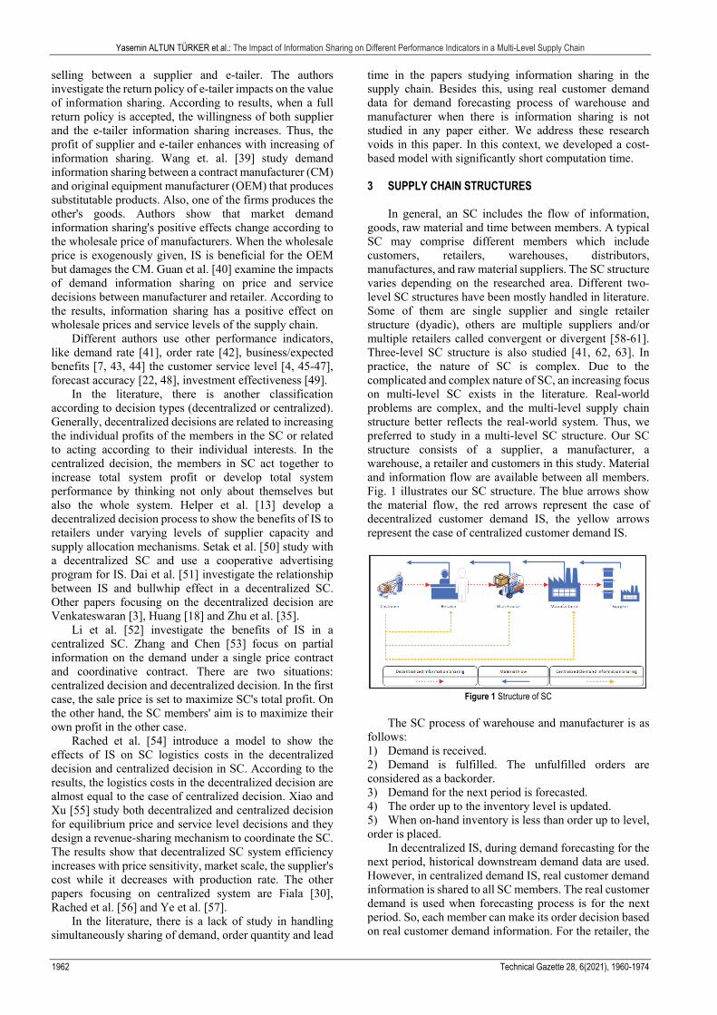
In general, an SC includes the flow of information, goods, raw material and time between members. A typical SC may comprise different members which include customers, retailers, warehouses, distributors, manufactures, and raw material suppliers. The SC structure varies depending on the researched area. Different two-level SC structures have been mostly handled in literature. Some of them are single supplier and single retailer structure (dyadic), others are multiple suppliers and/or multiple retailers called convergent or divergent [58-61]. Three-level SC structure is also studied [41, 62, 63]. In practice, the nature of SC is complex. Due to the complicated and complex nature of SC, an increasing focus on multi-level SC exists in the literature. Real-world problems are complex, and the multi-level supply chain structure better reflects the real-world system. Thus, we preferred to study in a multi-level SC structure. Our SC structure consists of a supplier, a manufacturer, a warehouse, a retailer and customers in this study. Material and information flow are available between all members. Fig. 1 illustrates our SC structure. The blue arrows show the material flow, the red arrows represent the case of decentralized customer demand IS, the yellow arrows represent the case of centralized customer demand IS.

Figure 1 Structure of SC

The SC process of warehouse and manufacturer is as

follows: 1) Demand is received. 2) Demand is fulfilled. The unfulfilled orders are considered as a backorder. 3) Demand for the next period is forecasted. 4) The order up to the inventory level is updated. 5) When on-hand inventory is less than order up to level, order is placed.

In decentralized IS, during demand forecasting for the next period, historical downstream demand data are used. However, in centralized demand IS, real customer demand information is shared to all SC members. The real customer demand is used when forecasting process is for the next period. So, each member can make its order decision based on real customer demand information. For the retailer, the



process of ordering is as follows: Retailer receives customer demand and calculates the order amount to be given to the warehouse by considering the situation in which there is sharing or no sharing. Then, the retailer places an order, updates the inventory level and waits for future customer demand for the next period. 3.1 Inventory Policy

The order up to policy is used for the inventory control system in our study. This policy is preferred by researchers because of its being easy to understand [64]. In order up to policy, the inventory level is observed periodically and checked whether the inventory is at the desired level. If the inventory is below the desired level, an order is placed to bring the inventory to the desired level. This order given at the end of each period is called the order up to inventory level (Yt). Eq. (1) represents a mathematical formula of Yt

developed by Chen et al. [65] LtX The estimate of mean

demand per period over L periods, Lt The estimate of

standard deviation of the demand over L periods, Z = A constant value to meet a desired service level):

L Ltt tY X Z (1)

Dejonckheere et al. [66] developed this formula by

inflating the lead time L by one unit and setting z = 0. Eq. (2) represents this new formula. In this study, we update the Eq. (2) and use this formula to calculate order up to inventory level for warehouse and manufacturer. We

present these equations in the formulations section tX

The estimate of the demand per period).

1 ttY L X (2)

3.2 Demand Forecasting

We prefer the exponential smoothing forecast method in this study. This method is easily understandable by the practitioners and has relatively simple mathematical expression form. The method is also one of the most preferred in the literature. Basically, the exponential smoothing method bases on adjusting the past estimation by weighting the forecast error [22]. Eq. (3) shows the used exponential smoothing formula [67]. X(t−1) denotes the actual demand for period (t − 1). α is the forecast smoothing factor and it means the weighting factor of the exponential smoothing rule where the value of α is between 0 and 1. The higher the value of α means that the greater is the weight placed on the more recent demand [42].

11 1 tt tX X X (3)

3.3 Ordering Decisions

In this study, the order quantity for warehouse and manufacturer depends on the order up to the level and actual demand for period t. At the end of period t, the

quantity of the order is given as Eq. (4). For the retailer order quantity is based on demand, inventory level and daily consumption rate. It is described in the following sections.

1 t ttOrder quantity Y Y X (4)

4 METHODOLOGY

In the literature, there are several theories about SC modelling. The selection of the modelling approach can change according to the studied problem and SC structure. Most of the papers in the literature used analytical models and simulation. SC structures have various properties and different constraints. By using analytical models including mathematical modelling and simulations under different scenarios, the complex structures of SC can be modelled and the effects of IS can be analysed [18, 34, 43, 68].

Our model is inspired by Rached et al.'s [17] model. Unlike their model, we added demand forecasting formulas and order up to level formulas under decentralized and centralized demand information shared. A new sharing type named order quantity and a new SC member named manufacturer are added into the model and the model is analysed for both decentralized and centralized situations. We represent our model as follows: Notations: t Replenishment period (t: {1, 2, 3, …, T}, P Number of days in a period, CD Customer demand, LT Lead time between manufacturer and warehouse, CDt Actual customer demand for period t(μCD, σCD), CD't Communicated demand in the case where the

demand is shared in period t, CDt Difference between the actual demand and

communicated demand in period CD CDt , ,

LTt Actual replenishment lead time between the manufacturer and warehouse in period t(μLT, σLT),

LT't Communicated replenishment lead time between the manufacturer and warehouse in period t,

LTt Difference between the actual lead time and

communicated lead time in period LT LTt , ,

μl Mean lead time between warehouse and retailer, σl Standard deviation of lead time between

warehouse and retailer, μs−m Mean lead time between supplier and

manufacturer, crt Daily consumption rate (If perfect knowledge of

demand is known), cr't Daily consumption rate (If CD is shared), crfix Daily consumption rate (If CD is not shared),

rtO Retailer order quantity in period t, wtO Warehouse order quantity in period t, mtO Manufacturer order quantity in period t,

wtO Warehouse demand forecasting in period t,

rtBO Backlogged retailer order quantity by warehouse,



mtO Manufacturer demand forecasting in period t,

wtBO Backlogged warehouse order quantity by

manufacturer, w

tY Warehouse order up to level in period t, m

tY Manufacturer order up to level in period t, rI Initial retailer inventory level, rtI Retailer inventory level at the end of period t, wI Initial warehouse inventory level, wtI Warehouse inventory level at the end of period t, mI Initial manufacturer inventory level, mtI Manufacturer inventory level at the end of period

t tsC Total system cost (manu. +ware. + retail.), trC Retailer total cost, twC Warehouse total cost, tmC Manufacturer total cost,

rtHC Retailer holding cost in period t, wtHC Warehouse holding cost in period t, mtHC Manufacturer holding cost in period t,

rtK Retailer ordering cost in period t, wtS Warehouse ordering cost in period t,

mtM Manufacturer ordering cost in period t,

rtP Retailer penalty cost in period t, w

tP Warehouse penalty cost in period t, m

tP Manufacturer penalty cost in period t, rhc Retailer holding cost per unit per day, whc Warehouse holding cost per unit per day, mhc Manufacturer holding cost per unit per day,

ro Retailer ordering cost, wo Warehouse ordering cost, mo Manufacturer ordering cost, rp Retailer penalty cost per unit per day, wp Warehouse penalty cost per unit per day, mp Manufacturer penalty cost per unit per day, rZ Retailer service level coefficient,

α Forecasting constant, CDSs Retailer safety stock if CD is shared

Ss Retailer safety stock if information is not shared, Assumptions:

This study considers a single-product, multi-stage, multi-period SC structure. The used information follows a normal distribution. LT is independent of the quantity dispatched. Suppliers can provide manufacturers with sufficient raw materials.

Formulations Order quantity in the case of sharing or no sharing:

Eq. (5) to Eq. (8) formulate the ordered amount by retailers in period t. It depends on customer demand (mean or real demand), safety stock, inventory level and daily consumption rate.

1 1r CD rt t l lt

't t l

'O CD Ss c Ir cr

(5)

1r rt CD l fox l t t l

O Ss cr cr I

(6)

CDlS P Ss

P

(7)

1rt

rlt S IO (8)

Eq. (5) determines the order quantity in only demand

sharing. Eq. (6) calculates the order quantity in only lead time between manufacturer and warehouse sharing. If there is no sharing, order up to inventory policy is adopted. Firstly, the replenishment level "S" is determined by Eq. (7), then order quantity is calculated Eq. (8). For t = 1,

1rtI is replaced by Ir.

To calculate order quantity, we need to know safety stock due to retailer inventory policies. We can calculate safety stock by Eq. (9) in the event demand sharing and by Eq. (10) in no sharing situation. The daily consumption rates change according to sharing or no sharing policies. Eq. (11) shows the daily consumption rate in period t due to real customer demand. If there is no sharing, Eq. (12) is used and if CD is shared, Eq. (13) is used for daily consumption rate. In the process of demand sharing, information may not always be accurate and reliable because of incomplete and incorrect communication between links. Therefore, a margin of error has been added to the value. Eq. (14) shows the communicated demand in demand sharing.

2

2 2CD r l CDlCD

Ss ZP P

(9)

2

2 2r l CDlCD

Ss ZP P

(10)

t tcr CD P (11)

fix CDcr P (12)

t'

t'cr CD P (13)

CD

t'

t tCD CD (14)

The manufacturer's and warehouse's order quantity are

based on their own internal customer demand (warehouse order quantity and retailer's order quantity, respectively) and order up to level. We mentioned that the order up to



level is upon the demand forecast. Hence, in decentralized or centralized sharing cases, calculated order quantities differ from each other. Eq. (15) and Eq. (16) show the calculation of order quantity of warehouse and manufacturer, respectively.

1w w w rt t ttO Y Y O (15)

1m m m wt t ttO Y Y O (16)

Demand forecasting in decentralized sharing: In decentralized sharing, when warehouse estimates

retailer's demand for the next period, historical retailer demand data are used. Likewise, while the manufacturer estimates the warehouse's demand for the next period, historical warehouse's demand data are used. We have shown the general demand forecast equation (Eq. (3)) in Section (3.2). We modified this equation as follows. Eq. (17) shows the estimation of the warehouse in period t and Eq. (18) shows the estimation of the manufacturer in period t.

1 11w r wt t tO O O (17)

1 11m w mt t tO O O (18)

Demand forecasting in centralized sharing: In centralized IS, demand is shared among all SC

members. The customer demand is used during demand forecasting for the next period. So, the manufacturer and the warehouse can make their order decision based on communicated customer demand data. Eq. (19) and Eq. (20) calculate the estimation of demand for warehouse and manufacturer, respectively.

11'w wt t tO CD O (19)

11'm mt t tO CD O (20)

Order up to level in the case of no sharing: As we mentioned above, Eq. (2) is adapted in our

model. Thus, Eq. (21) and Eq. (22) are obtained for order up to level for warehouse and manufacturer when there is no lead time or order quantity sharing.

w

w tt LT

OY P

P (21)

m

m tt s m

OY P

P (22)

Order up to level in the case of lead time sharing: If the warehouse knows the manufacturer's lead time,

it can determine order up to level according to this information. If lead time is sharing, LT't is replaced by μLT in Eq. (21) and Eq. (23) is obtained for warehouse order up

to level calculation. The LT information may not always be correct, so Eq. (24) is used for calculation.

w

w tt t

' OY P LT

P (23)

LT

t'

t tLT LT (24)

Order up to level in the case of order quantity sharing: Manufacturer updates the order up to inventory level

for the next period based on the estimate of the warehouse demand per period. In the case of sharing, the previous

period's order quantity is used for calculations. 'twO is used

instead of mtO and μs−m is replaced by μL in Eq. (22). Thus,

the Eq. (25) is obtained for calculation of manufacturer

order up to inventory level. 'twO is determined by Eq. (26)

based on error and real quantity.

w

w tt s

'

mO

Y PP

(25)

Inventory levels in the case of sharing or no sharing: Eq. (26) to Eq. (29) are the equations where the

warehouse updates the inventory level. According to the earliest delivery or lateness of delivery, the equations used can be changed. The variability in delivery dates is created by using μLT instead of LTt in the case where "LT" is not shared. In the event of sharing, the same equations are used

but t'LT is replaced instead of μLT.

1If then w w w rt LT t t ttLT I I O O (26)

1If then w w w rt LT t t ttLT Tt L

LT I I O O (27)

1If then w w wt LT t ttLTLT t

LT I I O (28)

If then w w rt LT t LTt tLTt

LT I I O (29)

The retailer updates the inventory level twice in the

replenishment period. The first update is determined by using Eq. (30) and the second update is calculated by Eq. (31). The manufacturer updates the inventory level by Eq. (32).

1 l tlr rt tI P crI (30)

1 11

rtl t t

r

l t

rtt

I I cr O

(31)

1m m w

tt ttmO OI I (32)

The calculation of total system cost:



If an order occurs in SC, the total ordering cost at retailer, warehouse and manufacturer is determined by Eq. (33), Eq. (34) and Eq. (35) respectively.

i 0 then f =0rr r rt ttK o KO (33)

i 0 then f =0ww w wt ttS o SO (34)

i 0 then f =0mm m mt ttM o MO (35)

When lead time is not shared, the holding cost of the

warehouse is calculated by Eq. (36) to Eq. (39) and Eq.

(40). If the value of lead time is shared, we used t'LT in

these equations instead of μLT. When LTtLT first the

cost incurred during LT tP LT is calculated by

Eq. (38) and then the cost incurred in the rest of period is

calculated by Eq. (39). For t = 1, 1wtI is changed by Iw.

1If then w w wt LT t tLT HC hc P I (36)

1If then w w wt LT t t LTtLT HC hc I P LT (37)

1If then w w wt LT t LT ttLT HC hc I P LT

(38)

If then w w

t LT t t

w wLT tt LTLT t

LT HC HC

hc I LT

(39)

1 w w w

t LT t t

wLT tt LTLT t

HC hc P LT I

I LT

(40)

Notice: Max , 0X X

Retailer holding cost is determined depending on inventory, holding cost (unit/day) and the consumption during period t. Eq. (41) calculates the cost incurred during P − μl. Eq. (42) calculates the cost incurred for the rest of the period. Eq. (43) calculates manufacturer holding costs.

For t = 1, 1mtI is changed by Im.

0

1 1

2

1

tr rt tP l lr rl

t

t

i

i cr i crI IHC hc

(41)

1

0

1 1

2

1r rt tt ttr r r

t t i

i crI IHC HC c

rh

i c

(42)

1 m m mt tHC hc P I (43)

When demand is not shared, a penalty cost can occur

at the retailer. Because, during the ordering process retailer determines the order quantity according to μCD and crfix. But maybe it can be less than the quantity required. In

sharing case, we μCD by CDt and crfix by 1'tcr . The retailer

penalty cost is calculated by Eq. (44) based on daily consumption during (P – μl) period. Eq. (45) determines the penalty cost during the rest of the period. There can be two penalty costs at the warehouse. One of these can be caused by backlogged orders and determined with Eq. (46). The other occurs if the lead time is greater than mean lead time and this penalty cost is calculated by Eq. (47). When

there is sharing, t'LT is used instead of μLT in the equation.

Eq. (48) represents the manufacturer penalty costs.

1r r r

l tt t ltP p P cr I

(44)

1r

lr r r

t tt t t IP P p cr

(45)

tw

t LTw rBOP p (46)

rLT

w wtt tP LT p O (47)

mm

tw

s tm OP p B (48)

Eq. (49) represents the total system cost. Eq. (50), Eq.

(51) and Eq. (52) present the total cost of the retailer, warehouse and manufacturer respectively.

t t t ts m w rC C C C (49)

1

Tt r r rr t t t

t

C HC K P

(50)

1

Tt w w ww t t t

t

C HC S P

(51)

1

Tt m m mm t t t

t

C HC M P

(52)

5 EXPERIMENTAL STUDIES

In this section, we display the model algorithm, model parameters and experimental results. The algorithm includes different stages based on IS type. 5.1 Model Algorithm and Parameters

Firstly, a data set consisting of customer demand and lead times is generated by using probability distributions in Tab. 1. For all scenarios, the same data set is used. All steps in the algorithm are continued for the specified period. The system operation is stopped when the last period is reached. All results are reported.



Table 1 Input data for model parameters Parameters Value Unit

t = {1, …, T} 30 - R 30 Days μCD 1200 - σCD 100 -

CD 0,05 -

CD 8 -

μLT 8 Days σLT 1 Day

LT 0,05 -

LT 1 -

μl 6 Days σl 1 Day

μs−m 4 Days

σs−m 0,50 Day

Zr 1,65 - α 0,05 - or 120 TL ow 150 TL om 100 TL hcr 0,03 TL/per day hcw 0,01 TL/per day hcm 0,01 TL/per day pr 0,125 TL/per day pw 0,125 TL/per day pm 0,125 TL/per day

wtO 270 -

mtO 100 -

TL: Turkish Liras

The different unit costs for each chain member,

statistical data required to generate random demand and lead times are seen in Tab. 1. Our planning horizon (T) consists of 30 periods. Every period includes 30 days. In this study, the safety stock level is accepted as 95%.

The scheme of the model algorithm is illustrated in Fig. 2. As seen in Fig. 2, firstly random values are generated by using the statistical data in Tab. 1. Then, the process proceeds as follows: Retailer receives customer demand. It is decided whether this demand will be shared between the SC members. If it is shared, we continue from the centralized demand sharing step. If it is not shared, we continue from the decentralized sharing step. In centralized demand sharing and decentralized sharing, the retailer order quantity is determined with Eq. (5) and Eq. (7) respectively. In the meantime, it is decided whether manufacturer-warehouse lead time will be shared. If it is shared, the retailer's order quantity is determined with Eq. (6). Retailer ordering cost is calculated by using Eq. (33). The retailer's inventory level is also updated by Eq. (30). Then, we calculate the retailer's holding cost with Eq. (41). The retailer's inventory level is updated again. Eq. (31) is used for this update. The holding cost of the retailer is recalculated by using Eq. (42). Then, the retailer's penalty cost is determined with Eq. (45).

After the warehouse receives the retailer's demand, the warehouse inventory level is controlled and if there is enough inventory, the desired amount is sent to the retailer. But, if it is not enough, the order becomes backlogged

order rtBO . Because of unfulfillment of retailer orders,

a penalty cost occurs at the warehouse and this cost is calculated by Eq. (46). In this equation the backlogged

order rtBO is determined according to the following

condition:

If then w r r r wt t t t tI O BO O I

If then 0w r rt t tI O BO

At this step, we query again whether there is centralized demand sharing or decentralized sharing. In centralized demand sharing, the warehouse forecasts the retailer's demand for next period by using Eq. (19). In the other case, this estimation is made with Eq. (17). In the meantime, it is decided whether manufacturer-warehouse lead time will be shared. If there is lead time sharing, we use Eq. (23) to update order up to the level for the next period. If LT is not shared, this level is updated by using Eq. (21).

Then, the warehouse's order quantity is determined with Eq. (15). Warehouse's ordering cost is calculated by using Eq. (34). Then, lead times are compared according to the studied scenario. In the sharing scenario, actual lead time (LTt) is compared with the communicated lead time (LT't). In the no sharing scenario, actual lead time (LTt) is compared with the mean lead time (μLT). Because of differences between the lead times, three different situations are handled: LTt < ( μLT or LT't): The warehouse order quantity requested from the manufacturer is received earlier than planned. Warehouse's inventory level is updated by Eq. (28). Then, we calculate the warehouse's holding cost with Eq. (38). Warehouse's inventory level is updated again with Eq. (29). The warehouse's holding cost is determined with Eq. (39). LTt = ( μLT or LT't)The warehouse order quantity arrives at the right time. Warehouse's inventory level is updated by Eq. (26). The warehouse's holding cost is calculated with Eq. (36). LTt > ( μLT or LT't): The warehouse order quantity is received later than planned. Due to this delay, a penalty cost occurs at the warehouse. This delay cost is calculated by using Eq. (47). Then, the warehouse's inventory level is updated by Eq. (27). The warehouse's holding cost is calculated with Eq. (37).

When the manufacturer receives the warehouse's demand, the inventory level is checked by the manufacturer and if there is sufficient inventory, the desired quantity is sent to the warehouse. However, if there is not sufficient inventory, the order becomes backlogged

order wtBO . A penalty cost occurs at the manufacturer

due to the unfulfillment of warehouse orders. Penalty cost is calculated by Eq. (48). In this equation, the backlogged

order wtBO is determined according to the following

condition:

If then m w w w mt t t t tI O BO O I

If then 0m w wt t tI O BO

It is queried whether there is centralized demand

sharing or decentralized sharing at this step. The manufacturer uses Eq. (20) to estimate the warehouse's demand for the next period in centralized demand sharing. Eq. (18) is also used for the estimation process if there is



decentralized sharing. Eq. (25) and Eq. (22) are used to update order up to level according to sharing or no sharing of warehouse order quantity. Then, the manufacturer's order quantity is determined with Eq. (16). Eq. (35) is used to calculate the manufacturer's ordering cost. The manufacturer's inventory level is updated with Eq. (32).

The manufacturer's holding cost is calculated with Eq. (43).

Finally, if the system reached the desired period, the total cost of the system is calculated using Eq. (49) to Eq. (52). At the end of the processes, all results are displayed.

Start

Generate a data file with random

customer’s demand and lead

time

Calculate the retailer order

quantity. (Eq. 6)

Calculate the retailer order cost

(Eq. 33)

Update the retailer inventory level

(Eq. 30)

Update the retailer inventory level

(Eq. 31)

Calculate the retailer holding

cost(Eq. 40’)

t=T?

No ( Decentralized)

Is customer’s demand share?


quantity.(Eq. 7)


quantity. (Eq. 5)

Yes (Centralized)

Is manufacture (M)-warehouse(W) lead time

share?

No

Calculate the retailer penalty

cost(Eq. 42')

Centralized demand information sharing?

Forecast retailer’s demand for next period

(Eq. 19)

Yes

Forecast retailer’s demand for next period

(Eq. 17)No ( Decentralized)

M-W lead time sharing?

Update order up to level for next period

(Eq. 23)


(Eq. 21)

Yes

No

Warehouse receives retailer’s

demand

YesIs warehouse inventory

level enough to send demand?

Fulfill retailer demand

Backlog unfulfilled retailer

demand

No

Calculate the warehouse order

quantity(Eq. 15)

Calculate the warehouse order

cost(Eq. 34)

Yes

Calculate the retailer holding

cost(Eq. 40)

Compare LT with µLT

Update the warehouse

inventory level(Eq. 29)

<

Calculate the warehouse

holding cost (Eq. 38’)


inventory level (Eq. 29’)


holding cost (Eq. 38)






inventory level (Eq. 28)

Calculate the warehouse penalty

cost

(Eq. 43)



>=

Manufacturer receives

warehouse’s demand

Is manufactırer inventory level enough

to send demand?

Fulfill warehouse demand

Yes

No

Backlog unfulfilled warehouse demand

Centralized demand information sharing?

Forecast warehouse’s demand for next period

(Eq. 20)

Yes

Forecast warehouse’s demand for next period

(Eq. 18)

No ( Decentralized)

Is order quantity share?


(Eq.25)

Yes


(Eq. 22 )No

Calculate the manufacturer order

quantity(Eq. 16)

Calculate the manufacturer

order cost (Eq. 35)

Update the manufacturer


Calculate the manufacturer holding cost

(Eq. 41)

Calculate the total system costs

(Eq.44,45,46,47)Finish

Output results

Yes

Retailer receives customer demand

No (t=t+1)

M-W lead time sharing?

Yes

Compare LT with LT’

No

What the

comparison

results?

Calculate the manufacturer penalty cost

(Eq. 43)

Figure 2 Algorithm scheme

5.2 Model Algorithm and Parameters

Our model in this study is implemented by using JavaScript ES 6 and run on a notebook with Intel i3 Processor and 4 GB RAM. The model is coded according to the algorithm steps in Fig. 2. Firstly, random values are generated by using statistical data in Tab. 1. The model runs until the desired period. Fifteen different instances are generated randomly for each scenario. The results show an average of fifteen trials. The effects of IS for retailer, warehouse and manufacturer are determined by finding

cost differences between "sharing cases" and "no sharing case". We discuss results in the following.

The one-way ANOVA (single factor) is used in this paper with the 95% confidence interval to determine whether there is a significant difference between obtained costs from eight scenarios (Sce.). Because ANOVA is used to test hypotheses about whether there is a significant difference between the means of two or more groups [69].

Tab. 2 presents the costs of holding, ordering, penalty and retailer's, warehouse's, manufacturer's total cost for every scenario. The total cost of the system in sharing scenarios is lower than the scenario of no IS in Tab. 2. In

Eq. 49, 50, 51, 52

(Eq. 48) (Eq. 43)

(Eq. 41) (Eq. 42)

(Eq. 45)

(Eq. 39)

(Eq. 29)

(Eq. 38)

(Eq. 28)

(Eq. 27)

(Eq. 47)

(Eq. 26)



between Sce.1 and Sce.7, when there is simultaneous sharing, the costs generally decrease. The minimum cost is obtained in Sce.7 where there is simultaneous sharing of three information.

Firstly, tests of normality are performed for each cost. The costs for each scenario are observed to be normally distributed with 95% confidence. ANOVA is performed to test the following hypotheses:

H0: There is no statistically significant difference between costs from scenarios. H1: There is a statistically significant difference between costs from scenarios.

The results are not represented completely in this study because of space limitations. For all costs except the "Ordering Cost" alternative hypothesis (H1) is accepted (Sig. = 0,00). This means that the effect of IS on costs is statistically significant.

Table 2 Cost of system members and total system costs*

Sce. Sharing Type Retailer Costs Warehouse Costs Manufacturer Costs TSC HC OC PC TRC HC OC PC TWC HC OC PC TMC

1 CD 3868,9 3480 1851,5 9200,4 13771,6 4350 981,5 19137,3 27600,7 2900 27,6 30528,3 58866,0 2 LT 4443,5 3480 2395,5 10319,0 11494,7 4350 267,2 16173,2 23911,9 2900 25,3 26837,2 53329,4 3 QW 5871,2 3600 1941,3 11412,4 16319,0 4350 1358,8 22508,1 23270,7 2900 198,1 26368,8 60289,3 4 CD, LT 3795,1 3480 1708,4 8983,4 11944,2 4340 253,6 16573,8 24212,2 2900 38,2 27150,4 52707,6 5 CD, QW 3868,9 3480 1851,5 9200,4 13771,6 4350 981,5 19137,3 23223,3 2900 47,2 26170,5 54508,2 6 LT, QW 4443,5 3480 2395,5 10319,0 11494,7 4350 267,2 16173,2 21225,7 2900 34,6 24160,3 50652,6 7 CD, LT, QW 3795,1 3480 1708,4 8983,4 11944,2 4340 253,6 16573,8 19899,4 2900 117,8 22917,2 48474,4 8 No share 5871,2 3600 1941,3 11412,4 16319,0 4350 1358,8 22508,1 28035,0 2900 141,0 31075,9 64996,5

HC: Holding Cost, OC: Ordering Cost, PC: Penalty Cost, TRC: Total Retailer Cost, TWC: Total Warehouse Cost, TMC: Total Manufacturer Cost, TSC: Total System Costs *Average of 15 instances

We analyse the costs according to differences in sharing and no sharing scenarios. Cost gains are seen during sharing of information situations. Tab. 3 shows the

cost gains within the system partners. Tab. 4 also presents the cost gains of each system member within the total cost of the system.

Table 3 Cost gains of system members within themselves

Sce. Sharing type Retailer cost gain % Warehouse cost gain % Manufacturer cost gain % HC OC PC TRC HC OC PC TWC HC OC PC TMC

1 CD 34,10 3,33 4,63 19,38 15,61 0,00 27,77 14,98 1,55 0,00 80,43 1,76 2 LT 24,32 3,33 -23,40 9,58 29,56 0,00 80,34 28,14 14,71 0,00 82,06 13,64 3 QW 0,00 0,00 0,00 0,00 0,00 0,00 0,00 0,00 16,99 0,00 -40,50 15,15 4 CD, LT 35,36 3,33 12,00 21,28 26,81 0,23 81,34 26,37 13,64 0,00 72,91 12,63 5 CD, QW 34,10 3,33 4,63 19,38 15,61 0,00 27,77 14,98 17,16 0,00 66,52 15,79 6 LT, QW 24,32 3,33 -23,40 9,58 29,56 0,00 80,34 28,14 24,29 0,00 75,46 22,25 7 CD, LT, QW 35,36 3,33 12,00 21,28 26,81 0,23 81,34 26,37 29,02 0,00 16,45 26,25

HC: Holding Cost, OC: Ordering Cost, PC: Penalty Cost, TRC: Total Retailer Cost, TWC: Total Warehouse Cost, TMC: Total Manufacturer Cost *Average of 15 instances

Table 4 Cost gains of system members within total cost

Sce. Sharing type Retailer cost gain % in total system cost

Warehouse cost gain % in total system cost

Manufacturer cost gain % in total system cost

Total gain

HC OC PC TRC HC OC PC TWC HC OC PC TMC 1 CD 3,08 0,18 0,14 3,40 3,92 0,00 0,58 5,19 0,67 0,00 0,17 0,84 9,43 2 LT 2,20 0,18 -0,70 1,68 7,42 0,00 1,68 9,75 6,34 0,00 0,18 6,52 17,95 3 QW 0,00 0,00 0,00 0,00 0,00 0,00 0,00 0,00 7,33 0,00 -0,09 7,24 7,24 4 CD, LT 3,19 0,18 0,36 3,74 6,73 0,02 1,70 9,13 5,88 0,00 0,16 6,04 18,91 5 CD, QW 3,08 0,18 0,14 3,40 3,92 0,00 0,58 5,19 7,40 0,00 0,14 7,55 16,14 6 LT, QW 2,20 0,18 -0,70 1,68 7,42 0,00 1,68 9,75 10,48 0,00 0,16 10,64 22,07 7 CD, LT, QW 3,19 0,18 0,36 3,74 6,73 0,02 1,70 9,13 12,52 0,00 0,04 12,55 25,42

HC: Holding Cost, OC: Ordering Cost, PC: Penalty Cost, TRC: Total Retailer Cost, TWC: Total Warehouse Cost, TMC: Total Manufacturer Cost *Average of 15 instances

5.2.1 Comparison of Scenario 1, Scenario 2 and Scenario 3

with Scenario 8

When a single type of information is shared, as shown in Tab. 4, the maximum gain in terms of total cost belongs to Sce.2 where there is sharing of lead time. The cost gain is 17,95% when there is "LT" sharing within total gain. In Sce.2, the largest share in the cost gain of the system belongs to the warehouse with 54,30%. It can be seen in Tab. 5 which shows the distribution of gain between system members. The most cost reduction between warehouse costs is in penalty cost. That is, the gain obtained from the penalty cost is higher than the gain obtained from other internal costs of the warehouse. In this

case, the holding cost gain is 29,56%. But it has no effect on ordering cost (Tab. 3).

Table 5 Distribution of gains between supply chain members Scenario Number Sharing types Retailer Warehouse Manufacturer

1 CD 36,08 54,98 8,93 2 LT 9,37 54,30 36,33 3 QW 0,00 0,00 100,00 4 CD, LT 19,77 48,29 31,94 5 CD, QW 21,09 32,14 46,77 6 LT, QW 7,62 44,16 48,21 7 CD, LT, QW 14,70 35,92 49,38

As for the manufacturer, we obtain a gain of 36,33%

compared to Sce.8 (Tab. 5). Lead time sharing provides a



significant gain with 82,06% in the penalty cost while it has no effect on ordering cost in the manufacturer. Also, it affects holding costs. The gain is 14,71% compared to no sharing scenarios (Tab. 3).

A positive relationship between LT sharing and penalty cost, holding cost is observed. This sharing type has the most impact on penalty cost among warehouse and manufacturer costs.

The retailer has the lowest cost gain in Sce.2 and this gain is approximately 9% (Tab. 5). When we look at the distribution of gain, the holding cost has the maximum rate with 24,32% (Tab. 3). The sharing of lead time reduces ordering costs but increases penalty costs (Tab. 2).

The second highest cost gain belongs to Sce.1, that is, demand sharing. Demand sharing has a positive impact on warehouse costs with 54.98% and retailer costs with 36,08%. This effect is approximately 8,93% in the manufacturer (Tab. 5).

According to Tab. 3 we can say that there is no impact of demand sharing on ordering cost of warehouse, but it has positive effects on penalty and holding costs. In terms of the retailer, holding cost gain has the most portion in total cost gain. Besides this, the gains of ordering cost and penalty cost are approximately close to each other. The impact of demand sharing on the manufacturer is low. The biggest share in this effect is the 80,43% gain in penalty cost.

Ordering cost sharing only affects the manufacturer costs. It provides holding cost gain of 16,99% compared to Sce.8 (Tab. 3). Although the penalty cost increases, the total cost of the manufacturer decreases (Tab. 2). 5.2.2 Comparison of Scenario 4, Scenario 5, Scenario 6 and

Scenario 7 with Scenario 8

When we analyse simultaneous IS the total system cost is lower than the costs of a single type of sharing scenarios and Sce.8 (Tab. 2). Sce.7 has the highest portion of the total cost gain of the system with a ratio of 25,42% (Tab. 4). In this scenario, the most profitable system member is the manufacturer. The cost gain of the manufacturer is 49,38%. The others are the warehouse (34,92%) and the retailer 14,70%, respectively (Tab. 5).

The simultaneous sharing of demand, lead time and order quantity significantly affect the warehouse penalty cost. The penalty cost gain is quite high with a gain 81,34%. The gain of holding cost is 26,81% but this sharing has little impact on ordering cost of the warehouse. As for the retailer, it is seen that a gain of 35,36% is obtained at holding cost, a gain of 12,00 % is obtained at penalty cost, a gain of 3,33% is obtained at ordering cost. For the manufacturer, the situation is as follows: The gain of holding cost is 29,02%. The gain of penalty cost is 16,45%. (Tab. 3) and there is no impact of Sce.7 on ordering the cost of the manufacturer.

Sce.6 has a portion of 22,07% in total gain (Tab. 4). In this case where the OQ and LT are shared simultaneously, the cost gain of warehouse and the manufacturer is close to each other. But retailer cost gain is lower than those (Tab. 5) In this scenario, the warehouse has the highest cost gain with 80,34%, which is penalty cost gain. The second highest cost gain is the penalty cost of the manufacturer (75,46%) and the third is holding cost gain at the

warehouse (29,56%). The gains of holding costs at the retailer and the manufacturer are approximately 25% (Tab. 3). The simultaneous sharing of OQ and LT does not affect the ordering cost of warehouse and manufacturer while it affects the retailer ordering cost (Tab. 3).

The cost gain rates at Sce.4 and Sce.5 compared to Sce.8 are 18,91%, 16,14% respectively (Tab. 4). In Sce.4, the highest cost gain is seen in the warehouse with 48,29 %. Manufacturer cost gain is in the second place with 31,94%. The retailer obtains a gain of 19,77% (Tab. 5). The highest share of warehouse and manufacturer cost gains belongs to the penalty cost. Holding cost gains are 26,81% and 13,64%, respectively. At the retailer, all costs are reduced so the cost gain is seen at every cost (Tab. 3).

In Sce.5, the highest cost gain is seen at the manufacturer with 46,77%. It is followed by the warehouse with 32,14%. At the retailer, a gain of 21,09% is obtained (Tab. 5). The highest share of warehouse and manufacturer cost gains belongs to the penalty cost, there is no gain in order cost. Holding cost gains are 15,61% and 17,16%, respectively. In the retailer, all costs are reduced so the cost gain is seen at every cost (Tab. 3).

In summary, we obtain cost gains ranging from 25% to 10% of the total system costs by IS. Between demand, lead time and order quantity, lead time sharing gives the lowest cost. In the cases of IS, holding costs have the most cost gains for every system member. Simultaneous sharing (C, LT, QW) yields the lowest cost. Order quantity sharing only affects manufacturer costs. The IS reduces only ordering cost of the retailer, other member's ordering costs remain the same. The biggest share in the cost gains is demand sharing for the retailer, lead time sharing for the warehouse and order quantity sharing for the manufacturer. 5.2.3 Comparison of Centralized Demand Sharing and

Decentralized Demand Sharing

In centralized demand IS, the warehouse uses real customer demand information instead of historical data when forecasting the retailer orders for the next periods. Likewise, real customer demand information is used when forecasting the warehouse orders for the next periods at the manufacturer. In decentralized IS, during demand forecasting for the next period, historical data are used.

When comparing centralized and decentralized sharing, the difference between order quantity estimates is compared with actual order quantities. Fig. 3 and Fig. 4 illustrate order quantities comparisons at the warehouse and the manufacturer, respectively.

Figure 3 Differences between actual order quantity and the estimated order

quantity at the warehouse



Figure 4 Differences between actual order quantity and the estimated order

quantity at the manufacturer

When Fig. 3 and Fig. 4 are examined, it is seen that the difference is lower if there is centralized sharing. In other words, we can say that using the actual demand data can increase the accuracy of the demand forecasting. 5.2.4 Comparison of Different Number Of Samples

In order to observe the behaviour of our model with different numbers of test data sets, test samples detailed in Tab. 6 are generated and the average costs incurred by

operating our system with these data sets are examined. These costs are shown in Tab. 6.

When our model is run with different data sets, it is expected that the resulting costs are close to each other. The obtained results are analysed with ANOVA. The tested hypotheses are the following: H0: There is no statistically significant difference between costs from test instances. H1: There is a statistically significant difference between costs from test instances.

ANOVA results for test instances in Tab. 6 are as follows: Sig. values are 0,488 for TRC, 0,978 for TWC, 1,000 for TMC and 0,999 for TSC. This means, for all costs, the null hypothesis (𝐻 ) is accepted (Sig. > 0,05). This finding implies that there is no significant difference between costs from test instances. Looking at these results, it is seen that our model works properly.

Finally, the last column in Tab. 6 presents the computational time of each scenario in our developed program. Computational times are acceptable. In other words, the developed program can find solutions within acceptable computation time.

Table 6 Costs in different data sets. *

Test instances Cost type Sharing type Total computational time / second CD LT QW CD, LT CD, QW LT, QW CD, LT, QW No sharing

N = 5 TRC 9759,9 10314,9 11422,7 9540,7 9759,9 10314,9 9540,7 11422,7 34,56 TWC 18956,0 15974,8 22164,5 16492,5 18956,0 15974,8 16492,5 22164,5 TMC 30521,7 26823,8 26320,8 27168,1 26188,1 24138,5 23041,3 31036,8 TSC 59237,6 53113,4 59908,0 53201,4 54904,0 50428,2 49074,6 64624,0

N = 10 TRC 9435,1 10247,4 11430,5 9212,9 9435,1 10247,4 9212,9 11430,5 73,57 TWC 19078,9 16092,2 22726,5 16623,6 19078,9 16092,2 16623,6 22726,5 TMC 30542,9 26822,8 26352,7 27165,4 26174,2 24150,0 22926,7 31056,1 TSC 59056,8 53162,4 60509,7 53001,9 54688,2 50489,6 48763,2 65213,1

N = 15 TRC 9200,4 10319,0 11412,4 8983,4 9200,4 10319,0 8983,4 11412,4 111,73 TWC 19137,3 16173,2 22508,1 16573,8 19137,3 16173,2 16573,8 22508,1 TMC 30528,3 26837,2 26368,8 27150,4 26170,5 24160,3 22917,2 31075,9 TSC 58866,0 53329,4 60289,3 52707,6 54508,2 50652,6 48474,4 64996,5

N = 20 TRC 9469,3 10338,7 11452,8 9253,0 9469,3 10338,7 9253,0 11452,8 143,01 TWC 19220,7 16272,3 22424,8 16748,2 19220,7 16272,3 16748,2 22424,8 TMC 30564,0 26849,7 26394,9 27178,7 26189,4 24176,6 23008,1 31088,6 TSC 59254,0 53460,7 60272,5 53179,9 54879,4 50787,6 49009,3 64966,1

N = 25 TRC 9592,5 10270,1 11397,7 9370,5 9592,5 10270,1 9370,5 11397,7 204,47 TWC 19099,5 16146,2 22212,3 16397,1 19099,5 16146,2 16397,1 22212,3 TMC 30503,0 26828,3 26323,7 27146,0 26161,5 24151,5 23001,5 31029,2 TSC 59195,0 53244,6 59933,6 52913,7 54853,5 50567,8 48769,1 64639,1

N = 50 TRC 9544,9 10283,2 11434,5 9324,3 9544,9 10283,2 9324,3 11434,5 379,08 TWC 19036,0 16177,4 22503,6 16572,7 19036,0 16177,4 16572,7 22503,6 TMC 30532,3 26829,6 26346,4 27163,6 26179,5 24153,9 23009,7 31054,7 TSC 59113,2 53290,1 60284,5 53060,5 54760,4 50614,4 48906,6 64992,8

N: Number of tests, TRC: Total Retailer Cost, TWC: Total Warehouse Cost, TMC: Total Manufacturer Cost, TSC: Total System Costs * Average of instances

6 CONCLUSIONS

This paper studies IS in single product multi-stage SC. Various scenarios (single, simultaneous and no sharing) are analysed to show the importance of IS. We focus on investigating the influence of IS on SC costs and estimation of order quantity. Demand, warehouse order quantity and lead time between warehouse-manufacturer are used in sharing scenarios. The effects of IS for retailer, warehouse and manufacturer are determined by finding cost differences between "sharing cases" and "no sharing case". Also, we compare the order estimations of warehouse and manufacturer in centralized or decentralized sharing.

We obtain the maximum cost gain when simultaneously sharing of three types of information. Among demand, lead time and order quantity, lead time sharing provides the lowest cost. Demand is second and order quantity is third in terms of low cost. Between different costs, the most reduction is seen at holding costs in whole system members.

Cooperation between the retailer and the warehouse can be considered because the maximum benefit is obtained from demand and lead time sharing. When these two types of information are shared, whole system members are provided gain. But order quantity sharing only affects the manufacturer cost compared to other system members. Our research demonstrates that the



retailer and the warehouse in SC could not receive profit from the order quantity IS.

The results obtained from ANOVA proved that the effect of IS on costs is statistically significant. Similarly, when the developed model is run with the different number of test instances, similar cost values are obtained.

It is seen that in centralized demand sharing, forecasting accuracy increases compared to decentralized sharing. Because, during centralized sharing, the actual customer data is used for the forecasting process. This demonstrates the sharing importance of customer demand information with all SC members.

More retailers, warehouses and manufacturers can be added in future studies. Different inventory policies or stock constraints can be incorporated into IS. A cooperation mechanism between SC members can be conducted for IS. In addition, papers can also be studied on how the bullwhip effect changes with IS. 7 REFERENCES [1] Simatupang, T. M. & Wright, A. C. (2002). The knowledge

of coordination for supply chain integration. Business Process Management Journal, 8(3), 289-308. https://doi.org/10.1108/14637150210428989

[2] Khanjari, N., Iravani, S., & Shin, H. (2017). Demand Information Sharing in a Supply Chain of Durable Goods with Pricing Decisions. SSRN Electronic Journal. https://doi.org/10.2139/ssrn.3032748

[3] Venkateswaran, J. & Son, Y. J. (2004). Impact of modelling approximations in supply chain analysis-an experimental study. International Journal of Production Research, 42(15), 2971-2992. https://doi.org/10.1080/00207540410001688392

[4] Chen, M. C., Yang, T., & Yen, C. T. (2007). Investigating the value of information sharing in multi-echelon supply chains. Quality & Quantity, 41(3), 497-511. https://doi.org/10.1007/s11135-007-9086-2

[5] Shih, S. C., Hsu, S. H. Y., Zhu, Z., & Balasubramanian, S. K. (2012). Knowledge sharing a key role in the downstream supply chain. Information & Management, 49(2), 70-80. https://doi.org/10.1016/j.im.2012.01.001

[6] Choi, T. M., Li, J., & Wei, Y. (2013). Will a supplier benefit from sharing good information with a retailer? Decision Support Systems, 56(1), 131-139. https://doi.org/10.1016/j.dss.2013.05.011

[7] Chengalur-Smith, I., Duchessi, P., & Gil-Garcia, J. R. (2012). Information sharing and business systems leveraging in supply chains: An empirical investigation of one web-based application. Information & Management, 49(1), 58-67. https://doi.org/10.1016/j.im.2011.12.001

[8] Cho, D. W. & Lee, Y. H. (2013). The value of information sharing in a supply chain with a seasonal demand process. Computers & Industrial Engineering, 65(1), 97-108. https://doi.org/10.1016/j.cie.2011.12.004

[9] Kumar, R. S. & Pugazhendhi, S. (2012). Information Sharing in Supply Chains: An Overview. Procedia Engineering, 38, 2147-2154. https://doi.org/10.1016/j.proeng.2012.06.258

[10] Dwaikat, N. Y., Money, A. H., Behashti, H. M., & Salehi-Sangari, E. (2018). How does information sharing affect first-tier suppliers' flexibility? Evidence from the automotive industry in Sweden. Production Planning and Control, 29(4), 289-300. https://doi.org/10.1080/09537287.2017.1420261

[11] Huang, Y. & Wang, Z. (2017). Values of information sharing: A comparison of supplier-remanufacturing and manufacturer-remanufacturing scenarios. Transportation Research Part E: Logistics and Transportation Review, 106, 20-44. https://doi.org/10.1016/j.tre.2017.07.015

[12] Barroso, A. P., Machado, V. H., & Machado, V. C. (2014). Demand information sharing impact on supply chain management under demand uncertainty. A simulation model. IEEE International Conference on Industrial Engineering and Engineering Management, 924-928. https://doi.org/10.1109/IEEM.2013.6962547

[13] Helper, C. M., Davis, L. B., & Wei, W. (2010). Impact of demand correlation and information sharing in a capacity constrained supply chain with multiple-retailers. Computers & Industrial Engineering, 59(4), 552-560. https://doi.org/10.1016/j.cie.2010.06.014

[14] Lee, H. L., So, K. C., & Tang, C. S. (2000). The Value of Information Sharing in a Two-Level Supply Chain. Management Science, 46(5), 626-643. https://doi.org/10.1287/mnsc.46.5.626.12047

[15] Ganesh, M., Raghunathan, S., & Rajendran, C. (2014). The value of information sharing in a multi-product, multi-level supply chain: Impact of product substitution, demand correlation, and partial information sharing. Decision Support Systems, 58(1), 79-94. https://doi.org/10.1016/j.dss.2013.01.012

[16] Shnaiderman, M. & Ouardighi, F. El. (2014). The impact of partial information sharing in a two-echelon supply chain. Operations Research Letters, 42(3), 234-237. https://doi.org/10.1016/j.orl.2014.03.006

[17] Rached, M., Bahroun, Z., & Campagne, J. P. (2015). Assessing the value of information sharing and its impact on the performance of the various partners in supply chains. Computers and Industrial Engineering, 88, 237-253. https://doi.org/10.1016/j.cie.2015.07.007

[18] Huang, Y. S., Li, M. C., & Ho, J. W. (2016). Determination of the optimal degree of information sharing in a two-echelon supply chain. International Journal of Production Research, 54(5), 1518-1534. https://doi.org/10.1080/00207543.2015.1092615

[19] Li, J. & Shaw, M. J. (2001). The Effects of Information Sharing Strategies on Supply Chain Performance. Proceedings of 8th ECIS, 3-5.

[20] Gonul Kochan, C., Nowicki, D. R., Sauser, B., & Randall, W. S. (2018). Impact of cloud-based information sharing on hospital supply chain performance: A system dynamics framework. International Journal of Production Economics, 195, 168-185. https://doi.org/10.1016/j.ijpe.2017.10.008

[21] Sabitha, D., Rajendran, C., Kalpakam, S., & Ziegler, H. (2016). The value of information sharing in a serial supply chain with AR(1) demand and non-zero replenishment lead times. European Journal of Operational Research, 255(3), 758-777. https://doi.org/10.1016/j.ejor.2016.05.016

[22] Trapero, J. R., Kourentzes, N., & Fildes, R. (2012). Impact of information exchange on supplier forecasting performance. Omega, 40(6), 738-747. https://doi.org/10.1016/j.omega.2011.08.009

[23] Tao, Y., Lai, X., & Zhou, S. (2020). Information sharing in a transparent supply chain with transportation disruptions and supplier competition. Annals of Operations Research, 1-23. https://doi.org/10.1007/s10479-020-03724-3

[24] Srivathsan, S. & Kamath, M. (2018). Understanding the value of upstream inventory information sharing in supply chain networks. Applied Mathematical Modelling, 54, 393-412. https://doi.org/10.1016/j.apm.2017.09.004

[25] Dominguez, R., Cannella, S., Barbosa-Póvoa, A. P., & Framinan, J. M. (2017). Information sharing in supply chains with heterogeneous retailers. Omega, 0, 1-17. https://doi.org/10.1016/j.omega.2017.08.005

[26] Huang, Z. & Gangopadhyay, A. (2004). A Simulation Study of Supply Chain Management to Measure the Impact of Information Sharing. Information Resources Management Journal, 17(3), 20-31. https://doi.org/10.4018/irmj.2004070102



[27] Yu, M. M., Ting, S. C., & Chen, M. C. (2010). Evaluating the cross-efficiency of information sharing in supply chains. Expert Systems with Applications, 37(4), 2891-2897. https://doi.org/10.1016/j.eswa.2009.09.048

[28] Davis, L. B., King, R. E., Hodgson, T. J., & Wei, W. (2011). Information sharing in capacity constrained supply chains under lost sales. International Journal of Production Research, 49(24), 7469-7491. https://doi.org/10.1080/00207543.2010.535037

[29] Ojha, D., Sahin, F., Shockley, J., & Sridharan S. V. (2019). Is there a performance tradeoff in managing order fulfillment and the bullwhip effect in supply chains? The role of information sharing and information type. International Journal of Production Economics, 208, 529-543. https://doi.org/10.1016/j.ijpe.2018.12.021

[30] Fiala, P. (2005). Information sharing in supply chains. Omega, 33(5), 419-423. https://doi.org/10.1016/j.omega.2004.07.006

[31] Tang, L., Yang, T., Tu, Y., & Ma, Z. (2020). Supply chain information sharing under consideration of bullwhip effect and system robustness. Flexible Services and Manufacturing Journal, 1-44. https://doi.org/10.1007/s10696-020-09384-6

[32] Byrne, P. J. & Heavey, C. (2006). The impact of information sharing and forecasting in capacitated industrial supply chains: A case study. International Journal of Production Economics, 103(1), 420-437. https://doi.org/10.1016/j.ijpe.2005.10.007

[33] Chu, W. H. J. & Lee, C. C. (2006). Strategic information sharing in a supply chain. European Journal of Operational Research, 174(3), 1567-1579. https://doi.org/10.1016/j.ejor.2005.02.053

[34] Iida, T. & Zipkin, P. (2010). Competition and Cooperation in a Two-Stage Supply Chain with Demand Forecasts. Operations Research, 58(5), 1350-1363. https://doi.org/10.1287/opre.1100.0809

[35] Zhu, W., Gavirneni, S., & Kapuscinski, R. (2009). Periodic flexibility, information sharing, and supply chain performance. IIE Transactions, 42(3), 173-187. https://doi.org/10.1080/07408170903394314

[36] Hall, D. C. & Saygin, C. (2012). Impact of information sharing on supply chain performance. The International Journal of Advanced Manufacturing Technology, 58(1-4), 397-409. https://doi.org/10.1007/s00170-011-3389-0

[37] Li, H., Pedrielli, G., Lee, L. H., & Chew, E. P. (2017). Enhancement of supply chain resilience through inter-echelon information sharing. Flexible Services and Manufacturing Journal, 29(2), 260-285. https://doi.org/10.1007/s10696-016-9249-3

[38] Feng, Y. (2012). System Dynamics Modeling for Supply Chain Information Sharing. Physics Procedia, 25, 1463-1469. https://doi.org/10.1016/j.phpro.2012.03.263

[39] Pei, Z. & Yan, R. (2019). Cooperative behavior and information sharing in the e-commerce age. Industrial Marketing Management, 76, 12-22. https://doi.org/10.1016/j.indmarman.2018.06.013

[40] Wang, J. J., Dong, J., Yue, X., & Zhong, Q. (2020). Information Sharing in a Supply Chain With a Coopetitive Contract Manufacturer. IEEE Transactions on Systems, Man, and Cybernetics: Systems, 50(5), 1777-1793. https:// doi.org/10.1109/TSMC.2017.2786867

[41] Guan, Z., Zhang, X., Zhou, M., & Dan, Y. (2020). Demand information sharing in competing supply chains with manufacturer-provided service. International Journal of Production Economics, 220(174), 1-10. https:// doi.org/10.1016/j.ijpe.2019.07.023

[42] Cannella, S., Framinan, J. M., & Barbosa-Póvoa, A. (2014). An IT-enabled supply chain model: a simulation study. International Journal of Systems Science, 45(11), 2327-2341. https://doi.org/10.1080/00207721.2013.769072

[43] Jeong, I. J. & Jorge Leon, V. (2012). A serial supply chain of newsvendor problem with safety stocks under complete and partial information sharing. International Journal of Production Economics, 135(1), 412-419. https://doi.org/10.1016/j.ijpe.2011.08.015

[44] Wang, J. C., Wang, Y. Y., & Che, T. (2019). Information sharing and the impact of shutdown policy in a supply chain with market disruption risk in the social media era. Information & Management, 56(2), 280-293. https://doi.org/10.1016/j.im.2018.09.005

[45] Li, J., Sikora, R., Shaw, M. J., & Woo Tan, G. (2006). A strategic analysis of inter organizational information sharing. Decision Support Systems, 42(1), 251-266. https://doi.org/10.1016/j.dss.2004.12.003

[46] Costantino, F., Di Gravio, G., Shaban, A., & Tronci, M. (2014). The impact of information sharing and inventory control coordination on supply chain performances. Computers & Industrial Engineering, 76, 292-306. https://doi.org/10.1016/j.cie.2014.08.006

[47] Xue, X., Shen, Q., Tan, Y., Zhang, Y., & Fan, H. (2011). Comparing the value of information sharing under different inventory policies in construction supply chain. International Journal of Project Management, 29(7), 867-876. https://doi.org/10.1016/j.ijproman.2011.04.003

[48] Wang, X. (2012). Research on the construction of supply chain collaboration system based on information sharing. 2012 International Conference on Information Management, Innovation Management and Industrial Engineering, 1, 469-472. https://doi.org/10.1109/ICIII.2012.6339704

[49] Zhang, Q., Tang, W., Zaccour, G., & Zhang, J. (2019). Should a manufacturer give up pricing power in a vertical information-sharing channel?. European Journal of Operational Research, 276(3), 910-928. https://doi.org/10.1016/j.ejor.2019.01.054

[50] Setak, M., Kafshian Ahar, H., & Alaei, S. (2018). Incentive mechanism based on cooperative advertising for cost information sharing in a supply chain with competing retailers. Journal of Industrial Engineering International, 14(2), 265-280. https://doi.org/10.1007/s40092-017-0225-7

[51] Dai, H., Li, J., Yan, N., & Zhou, W. (2016). Bullwhip effect and supply chain costs with low and high-quality information on inventory shrinkage. European Journal of Operational Research, 250(2), 457-469. https://doi.org/10.1016/j.ejor.2015.11.004

[52] Li, K., Liu, X.-Y., & Jacobson, D. (2018). Information and profit sharing between a buyer and a supplier: Theory and practice. Managerial and Decision Economics, 39(1), 79-90. https://doi.org/10.1002/mde.2870

[53] Zhang, J. & Chen, J. (2013). Coordination of information sharing in a supply chain. International Journal of Production Economics, 143(1), 178-187. https://doi.org/10.1016/j.ijpe.2013.01.005

[54] Rached, M., Bahroun, Z., & Campagne, J. P. (2016). Decentralised decision-making with information sharing vs. centralised decision-making in supply chains. International Journal of Production Research, 54(24), 7274-7295. https://doi.org/10.1080/00207543.2016.1173255

[55] Xiao, T. & Xu, T. (2013). Coordinating price and service level decisions for a supply chain with deteriorating item under vendor managed inventory. International Journal of Production Economics, 145(2), 743-752. https://doi.org/10.1016/j.ijpe.2013.06.004

[56] Rached, M., Bahroun, Z., Baboli, A., Campagne, J., & Zouari, B. (2009). A method to evaluate downstream and upstream information sharing using the genetic algorithm. 2009 International Conference on Computers & Industrial Engineering, 1635-1640. https://doi.org/10.1109/ICCIE.2009.5223809

[57] Ye, F., Qian, Y., & Hu, R. Q. (2016). A Real-Time Information Based Demand-Side Management System in



Smart Grid. IEEE Transactions on Parallel and Distributed Systems, 27(2), 329-339. https://doi.org/10.1109/TPDS.2015.2403833

[58] Aviv, Y. (2001). The Effect of Collaborative Forecasting on Supply Chain Performance. Management Science, 47(10), 1326-1343. https://doi.org/10.1287/mnsc.47.10.1326.10260

[59] Zhu, K. & Thonemann, U. W. (2004). Modeling the Benefits of Sharing Future Demand Information. Operations Research, 52(1), 136-147. https://doi.org/10.1287/opre.1030.0061

[60] Wu, J., Zhai, X., Zhang, C., & Liu, X. (2011). Sharing quality information in a dual-supplier network: a game theoretic perspective. International Journal of Production Research, 49(1), 199-214. https://doi.org/10.1080/00207543.2010.508947

[61] Barlas, Y. & Gunduz, B. (2011). Demand forecasting and sharing strategies to reduce fluctuations and the bullwhip effect in supply chains. Journal of the Operational Research Society, 62(3), 458-473. https://doi.org/10.1057/jors.2010.188

[62] Chen, F., Drezner, Z., Ryan, J. K., & Simchi-Levi, D. (2000). Quantifying the Bullwhip Effect in a Simple Supply Chain: The Impact of Forecasting, Lead Times, and Information. Management Science, 46(3), 436-443. https://doi.org/10.1287/mnsc.46.3.436.12069

[63] Dejonckheere, J., Disney, S., Lambrecht, M., & Towill, D. (2004). The impact of information enrichment on the Bullwhip effect in supply chains: A control engineering perspective. European Journal of Operational Research, 153(3), 727-750. https://doi.org/10.1016/S0377-2217(02)00808-1

[64] Disney, S. M. & Lambrecht, M. R. (2008). On Replenishment Rules, Forecasting, and the Bullwhip Effect in Supply Chains. Foundations and Trends® in Technology, Information and Operations Management, 2(1), 1-80. https://doi.org/10.1561/0200000010

[65] Lau, J. S. K., Huang, G. Q., & Mak, K. L. (2004). Impact of information sharing on inventory replenishment in divergent supply chains. International Journal of Production Research, 42(5), 919-941. https://doi.org/10.1080/00207540310001628911

[66] Li, T. & Zhang, H. (2015). Information sharing in a supply chain with a make-to-stock manufacturer. Omega, 50, 115-125. https://doi.org/10.1016/j.omega.2014.08.001

[67] Ortiz-Vargas, D. A. & Montoya-Torres, J. R. (2012). Programaci??n de la produccti??n baio un ambiente de colaboraci??n en una cadena de suministro di??dica. Ingenieria y Universidad, 16(2), 315-331.

[68] Sadeghi, A. (2015). Providing a measure for bullwhip effect in a two-product supply chain with exponential smoothing forecasts. International Journal of Production Economics, 169, 44-54. https://doi.org/10.1016/j.ijpe.2015.07.012

[69] Tabachnick, B. G. & Fidell, L. S. (2006). Using Multivariate Statistics (6th edition). Allyn & Bacon.

Contact information: Yasemin ALTUN TÜRKER, PhD (Corresponding author) Karabuk & Sakarya University, Engineering Faculty, Industrial Engineering Department, 78050, Karabuk, Turkey/54187, Sakarya, Turkey E-mail: [email protected] Tuğba TUNACAN, PhD, Assistant Professor Bolu Abant Izzet Baysal University, Engineering Faculty, Industrial Engineering Department, 14030, Bolu, Turkey E-mail: [email protected] Orhan TORKUL, PhD, Professor Sakarya University, Engineering Faculty, Industrial Engineering Department, 54187, Sakarya, Turkey E-mail: [email protected]

Documents

The Impact of Information Sharing on Different Performance