Received: 13 February 2018 Revised: 24 September 2018 Accepted: 17 October 2018

DOI: 10.1002/hec.3840

R E S E A R C H A R T I C L E

The impact of financial incentives on health and healthcare: Evidence from a large wellness program

Liran Einav1 Stephanie Lee2 Jonathan Levin3

1Department of Economics, StanfordUniversity, Stanford, California2Foster School of Business, University ofWashington, Seattle, Washington3Department of Economics and GraduateSchool of Business, Stanford University,Stanford, California

CorrespondenceLiran Einav, Department of Economics,Stanford University, Stanford, CA, USA.Email: Leinav@stanford.edu

Abstract

Workplace wellness programs have become increasingly common in the UnitedStates, although there is not yet consensus regarding the ability of such pro-grams to improve employees' health and reduce health care costs. In this paper,we study a program offered by a large U.S. employer that provides substan-tial financial incentives directly tied to employees' health. The program has ahigh participation rate among eligible employees, around 80%, and we analyzethe data on the first 4 years of the program, linked to health care claims. Wedocument robust improvements in employee health and a correlation betweencertain health improvements and reductions in health care cost. Despite thelatter association, we cannot find direct evidence causally linking program par-ticipation to reduced health care costs, although it seems plausible that such arelationship will arise over longer horizons.

KEYWORDS

health behavior, health care cost, wellness programs

1 INTRODUCTION

Workplace wellness programs have become an important tool for employers, insurers, and policymakers to combat risinghealth care costs. These programs stem from the idea that encouraging working individuals to adopt a healthier lifestyle isa “win-win” strategy. Wellness programs have the potential to lead to better health for the individuals involved, translateto improved labor productivity, and reduce health care costs (Alderman, 2009; Baicker, Cutler, & Song, 2010).

Although some form of wellness program is offered by the majority of large employers in the United States (see Mattkeet al., 2013, for a comprehensive review), there is not yet clear consensus as to the impact of such programs or as towhich program design features are most effective.1 Although the potential for cost saving appears large (Bolnick, Millard,& Dugas, 2013) and some studies suggest that wellness programs are associated with cost savings (Baicker et al., 2010;Ozminkowski, Ling, Goetzel, Bruno, Rutter, Isaac, & Wang, 2002), others do not find a significant effect on cost (Aldana,Merrill, Price, Hardy, & Hager, 2005; Caloyeras, Liu, Exum, Broderick, & Mattke, 2014; Jones, Molitor, & Reif, 2018) orworry that such programs shift costs onto less healthy employees (Horwitz, Kelly, & DiNardo, 2013). On March 23, 2010,

1Seventy-one percent of large firms with 200 or more employees with health benefits offer programs to help employees stop smoking, 68% offer lifestyleor behavioral coaching, and 61% offer programs to help employees lose weight. Eighty-one percent of large firms report offering at least one of thesethree programs (Claxton, Rae, Panchal, Whitmore, Damico, Kenward, & Long, 2015).

Health Economics. 2019;28:261–279. wileyonlinelibrary.com/journal/hec © 2018 John Wiley & Sons, Ltd. 261

262 EINAV ET AL.

President Obama endorsed a provision created to encourage employers to implement more substantial standard-basedwellness programs.

In this paper, we add to the existing evidence by exploiting rich administrative data from a large U.S. employer thathas been a pioneer in designing and implementing a workplace wellness program. The employer introduced its wellnessprogram in late 2008. The program is innovative in its design and offers large financial incentives. A central feature of theprogram is that financial incentives are directly linked to employees' health. Through its workplace wellness program,the employer provides its employees the strong financial incentives to pass specific health standards.

We describe the employer's workplace wellness program and the financial incentives, as well as our data, in Section2. The program tracks five common health measures once a year—body mass index (BMI), blood pressure, cholesterol,glucose, and nicotine. Our data contain administrative records for all eligible employees (and their program eligibledependents), as well as annual health measures for all program participants, and health insurance claim-level data formost individuals. We use data from the first 4 years of the program (2009–2012), covering more than 20,000 participantsper year. Participation rates among eligible individuals are higher than in most other programs. Perhaps the most uniquefeature of the program is its incentive structure. Although most employers offer participation payments for employees,the employer we examine ties financial incentives directly to biometric measurements, offering up to $1,000 per year forindividuals who do well on all metrics. The financial rewards (paid in the form of insurance premium discounts) can beeliminated entirely for individuals who fail all screenings.2

In Section 3, we use a variety of empirical approaches to document a robust year-to-year improvement in each mea-sured biometric for program participants. This complements findings reported in Fu, Bradley, Viswanathan, Chan, andStampfer (2016) for the same employer.3 There are two empirical challenges in attempting to attribute causal interpre-tation to the findings described above. First, participation in the program is voluntary, although internal advertising,benefits sessions, and the financial incentives lead to relatively high participation rates of 75–80% among eligible individ-uals. Second, health measures are only available for program participants during their participating years so cannot beassessed against nonparticipants. Although there is no perfect way to circumvent these challenges, we use external datato provide some benchmarks for comparison, which generally supports a causal interpretation.

An important part of the analysis in Section 3 is our ability to observe participating individuals for up to 4 years. Thismeans that not only we can assess the binary and immediate impact of program participation, which was the focus of allthe studies mentioned earlier but also we can focus on the possibility that the impact of the program may not be imme-diate and could be linked to consistent, year-after-year participation that may inhibit health-related habits for instance(Charness & Gneezy, 2009; Mochon, Schwartz, Maroba, Patel, & Ariely, 2016). In one specification, we compare the pass-ing rate of program participants between those new participants and individuals who have been participating in theprogram for several years, and we find that longer program participation is associated with significant and meaningfulimprovements in screening results, especially for men.

Section 4 relates these health improvements to health care cost and utilization. With a simple difference-in-differencesspecification, we do not find clear evidence that program participation is associated with lower health care cost, at leastover the first 4 years of the program, and this finding is consistent with the results of Jones et al. (2018), who find similarresults in a randomized control trial in a similar context. In fact, we find some evidence for higher health care cost over thefirst 2 years. However, we do present evidence that health improvements in terms of BMI and blood pressure (but not interms of cholesterol and glucose) are associated with lower health care utilization and cost, as well as empirical evidencethat the program triggers individuals to start treating (or adhere better) to their blood pressure and cholesterol-reducingdrugs.

In the final section, we summarize our findings and conclude. Overall, although we do not find clear evidence thathealth care cost has declined as a result of the wellness program, our overall conclusion is quite positive. Participatingemployees appear healthier, and this will likely make them more productive and perhaps even cheaper in the longer run,regardless of the shorter run cost-benefit analysis. Of course, our analysis and statistical inference rely on data from asingle program implemented in a single firm, and further studies with similar programs and other firms are needed toassess external validity.

2It is common for employer wellness programs to pay financial rewards in the form of premium discounts, as it is the case here. An interesting questionis whether the effect of financial incentives would be different if financial rewards were paid in cash or in other forms.3A related finding is reported by Cawley and Price (2013), who document a response by employees to financial incentives associated with weight loss.

EINAV ET AL. 263

2 SETTING AND DATA

2.1 The employer's workplace wellness programThe employer's workplace wellness program in its current form was first implemented for the calendar year 2009 andhas continued throughout our sample period with small changes from year to year. All nonunion employees are eligiblefor the program, as well as their spouses if they are covered (as dependents) by the employer's employer-provided healthinsurance. Participation in the program is voluntary and has been around 75–80% among all eligible individuals.

Program participation requires individuals to take an annual confidential health screening and have its results reportedto the program administration.4 The screening can either be taken in a doctor's office, with the results transmitted to thecompany, or more commonly, the program organizes and advertises prescheduled on-site events in which individualscould participate in the health screening session in their job location. Employees are informed about the wellness programthrough the company intranet and home mailer. Furthermore, human resources teams across the company are trained toensure that program information is accurately and effectively shared with employees. Employees have access to an onlinebenefits portal where screening details, scheduling dates, and deadlines are accessible.

The health screening session takes about 15–30 min and involves measuring five distinct health metrics and a sub-sequent optional consultation with a health professional. The five health metrics are BMI, blood pressure, cholesterol,glucose, and smoking. Each is associated with a pass/fail outcome. Passing standards are based on the standard healthguidelines, with some leeway relative to the National Institutes of Health (NIH) recommendations.

BMI is the ratio of the individual's weight (in kilograms) to the square of her height (in meters), with a BMI of 30 orbelow considered a passing result.5 Blood pressure is measured using the systolic and diastolic millimeter of mercuryreadings, with passing result requiring that the reading is both below 140 (systolic) and below 90 (diastolic). Cholesterolis measured by total cholesterol, with values below 220 mg/dl considered a passing result.6 To pass the glucose test (whichstarted in 2010), glucose must be below 116 mg/dl, and to check for smoking, individuals had to obtain a negative resulton a nicotine test.7

To the extent that financial incentives exist, the typical wellness programs provide such incentives by rewarding pro-gram participation. One of the unique features of the workplace wellness program at the employer we study is that thefinancial incentives to participants are large and are directly linked to successful test results. Each passing result on abiometric comes with a financial reward: a 3.00–5.50 dollar premium reduction in the weekly health insurance premium.These incentives can add up across five tests and a full calendar year to approximately 1,000 dollars per individual (or2,000 dollars per household with two participating adults). Moreover, the program provides even stronger incentives toindividuals who are less healthy. If an individual improves her health and meets the passing standard 1 year after hav-ing missed it in the prior year, she can receive a rebate for the measure retrospectively, so in such situations, financialincentives are doubled. Appendix A provides complete details of the program rules.

2.2 DataOur data include annual information on all the eligible employees and spouses over 5 years (2008–2012), starting in theyear before the start of the wellness program and covering the first 4 years in which the program has been in place. Inaddition to the health measures that are available for all program participants, we also obtained administrative data onthe employees' (and dependents) health insurance and pharmaceutical drug insurance claims for employees who areenrolled in the employer's preferred provider organization (PPO) health insurance plan.

Table 1 presents summary statistics. Our initial, full sample—summarized in column 1—consists of all individuals whowere eligible for the workplace wellness program, that is, all nonunion employees and their spouses who were covered bythe employer's employer-provided health insurance. This sample consists of 115,805 individual years that represent 41,590unique individuals, of which 30,724 are employees and the rest are covered spouses. Forty-six percent of the observationsare male, the average age is 45, and the majority have been working at the company for more than 10 years, with only

4Fifty percent of large firms with 200 or more employees with health benefits offer or require employees to complete an annual biometric screening(Claxton et al., 2015).5Pregnant women automatically pass. Individuals with high BMI results could also pass the BMI metric by showing a 10% reduction in BMI in thesubsequent year, even if the BMI is still above 30. Alternatively, individuals whose weight is high due to muscles buildup can elect to pass the BMImetric with waist circumference measure that is less than 40 (for males) or 35 (for females) in.6This is effective on 2011 and later. Cholesterol measurement did not take place in 2009, and in 2010, the requirements for a passing result weremore stringent (high-density lipoprotein has to be greater than 40 mg/dl, low-density lipoprotein to be less than 130 mg/dl, and triglyceride less than200 mg/dl).7The nicotine test result is binary, and the passing rate for those who take it is close to 100%, so we do not use this test throughout the analysis.

264 EINAV ET AL.

TABLE 1 Summary statistics

Full sample Health only Utilization only Complete data(1) (2) (3) (4)

ObservationsIndividual-years 115,805 85,673 91,153 61,021Unique individuals 41,590 34,212 32,939 24,640Unique employees 30,724 26,059 24,030 18,667

Demographic informationa

Male 0.46 0.45 0.46 0.45Ageb (average) 45.17 45.39 45.86 46.44Age,b (standard deviation) 11.80 11.80 11.53 11.23Salary (average, in $000) 58.43 61.95 58.87 61.95Salary (standard deviation) 37.32 38.20 37.14 38.20Year of hire, average 1997.6 1996.8 1997.3 1996.8Share hired in 2009 or later 0.078 0.056 0.064 0.056

State of employmentCalifornia 0.23 0.23 0.19 0.19Texas 0.17 0.17 0.20 0.20Oregon 0.16 0.16 0.16 0.16Other 0.44 0.44 0.45 0.45

Health expenditureAnnual health spending 5,117 4,865Standard deviation 19,668 17,911Percent zero 0.17 0.14Annual drug (RX) spending 789 947Standard deviation 3,159 3,079Percent zero 0.26 0.21

Healthy measures passing ratesBMI 0.76 0.75BP 0.85 0.85Cholesterol (2010–2012) 0.76 0.76Glucose (2010–2012) 0.86 0.86

Note. BMI: body mass index; BP: blood pressure. Observations are from 2009 to 2012. “Health only” sample includes all individuals whoparticipated in the healthy measures program that year. ”Utilization only” sample includes all individuals enrolled in one of the safewaypreferred provider organization options that year. “Complete data” sample includes individual years who satisfy both criteria above.aAge and gender information is available for everyone. Other information is missing for some individuals. Salary and hire information isbased on 82,116, 52,788, 75,712, and 52,788 in each sample, respectively. Location (state) information is based on 68,534, 68,534, 48,854,and 48,854 in each sample, respectively. bThere are 121 individuals whose age is 65+, but the exact age is unknown. We use 70 for theseindividuals to calculate the summary statistics.

7.8% who were hired in 2009 or after. The employer has a national presence and operates across the country, but morethan half of the sample contain individuals in California, Texas, and Oregon.

This initial sample has various elements of missing data for two primary reasons. First, health information is missingfor program nonparticipants as their health measures are not being recorded. These account for 26% of the individualyears in the sample. Second, eligible individuals may opt to enroll in a health insurance plan that is different from theemployer's PPO coverage. They are covered by Kaiser Permanente, which is a vertically integrated health care provider.It receives capitated payments from the employer and thus does not report back to the employer claim-level utilizationinformation. These individuals account for 21% of the individual years in the original sample.

We therefore end up working with different forms of samples, based on the specific analyses. The “health only”sample—summarized in column 2 of Table 1—includes all participating individuals for whom we have health measures,the “utilization only” sample—summarized in column 3—includes all PPO enrollees for whom we have utilization data,and the “complete data” sample (in column 4) is the intersection of the two. As Table 1 shows, the samples are reasonablysimilar in terms of their observables (gender, age, salary, tenure at the company, and job location). However, selection onunobservables (into the wellness program or into Kaiser coverage) is an important concern, and we will address it belowusing the different research designs and identification strategies.

EINAV ET AL. 265

3 HEALTH CHANGES OVER TIME

3.1 Health trends for program participantsIn this section, we use the health only sample to explore how health changes for program participants. We start by lookingat all individuals whose health is observed over consecutive years. That is, we drop individuals who are only in the samplefor a single year or for nonconsecutive years, and we treat each pair of consecutive years as a separate observation. Thus,for example, individuals who are observed for all 4 years are used to generate three different observations.

Table 2 shows the pass fail transition matrix for all consecutive year observations. As expected, health is highly corre-lated over time within an individual. Individuals who pass a given test in 1 year are much more likely to pass it in thesubsequent year, with passing rates ranging from 91 to 94% conditional on passing the same test in the previous year,whereas passing rates are much lower—18% for BMI and 45–65 for the other metrics—for those individuals who did notpass in the previous year.

Table 2 additionally points to likely improvements in health metrics over time, as the transition matrix is not symmetric:The rate by which individuals' transition from pass to fail is significantly lower than the rate by which they transitionedfrom fail to pass. To see this more granularly, Figure 1 presents the relationship between the health measure in a givenyear against the corresponding health measure of the same individual in the previous year. Across all measures, onecan observe a clear pattern: Individuals with high (worse) health metrics tend to have lower ones the year after, andindividuals with low health metric tend to have higher ones. It is important to note that high measures are bad, butconditional on being low enough, lower measures are not necessarily better. In this sense, Figure 1 shows a clear patternof improvements in health. To see this, note that we also plot the “passing threshold” in each panel of the figure, and inall panels, the pattern crosses the 45-degree line below the passing threshold (and often even below the more stringentNIH recommendation), implying that individuals whose health metrics are too high tend to improve on average.

The pattern described above suggests that individuals who participate in the program tend to get healthier, at least onaverage. Of course, this pattern does not mean necessarily that this improved health is caused by the program participa-tion. The improvement in health may be viewed as even less trivial once one realizes that aging alone should make manyhealth metrics deteriorate from year to year, rather than improve. Medical literature has found that blood pressure riseswith age, a phenomenon which is associated with structural changes in the arteries (Pinto, 2007). Cholesterol and glu-cose levels also tend to rise with age (Kannel, 1987; O'Sullivan, 1974). An important concern, however, is that the patternobserved in Figure 1 merely reflects mean reversion, either in true health or in the measurement of health. For example,a similar qualitative pattern could be generated if health is measured with error or if one's day-to-day health fluctuates(so a measurement in a particular day is a noisy signal of one's average daily health over the year).

To explore the potential importance of mean reversion and to more generally compare the pattern observed by theemployer we study to some other benchmarks, we have searched for other data sets that follow individuals' health

TABLE 2 Year-to-year passing rates

BMI Pass in year t Fail in year t Blood pressure Pass in year t Fail in year t

Pass in year t − 1 35,360 2,236 Pass in year t − 1 37,972 3,8490.94 0.06 0.91 0.09

Fail in year t − 1 1,983 8,777 Fail in year t − 1 4,185 2,3500.18 0.82 0.64 0.36

Cholesterol Pass in year t Fail in year t Glucose Pass in year t Fail in year tPass in year t − 1 19,229 1,927 Pass in year t − 1 21,403 1,229(actual standards) 0.91 0.09 (actual standards) 0.95 0.05Fail in year t − 1 6,141 4,287 Fail in year t − 1 6,739 2,213(actual standards) 0.59 0.41 (actual standards) 0.75 0.25Pass in year t − 1 22,034 2,317 Pass in year t − 1 26,152 1,571(2011 standards) 0.90 0.10 (2011 standards) 0.94 0.06Fail in year t − 1 3,336 3,897 Fail in year t − 1 1,990 1,871(2011 standards) 0.46 0.54 (2011 standards) 0.52 0.48

Note. Table presents observation counts in each cell (shares below the counts). An observation is an individual observed over twoconsecutive years. An individual who is observed over three or four consecutive years is included as two or three, respectively,multiple observations. Cholesterol and glucose measurement started in 2010 only, and passing standards were relaxed in 2011, sowe report above passing rates based on either actual standard or the relaxed 2011 standards.

266 EINAV ET AL.

FIGURE 1 The timing of preventive drug purchasing and screening results. Figure plots (thick black lines) predictions from kernelregression of a health indicator in 1 year on the same health indicator the year before, using all available observations on the same person inconsecutive years. Each panel presents one type of test. All panels show the 45-degree line, two vertical lines at the employer passingthreshold and the (lower) National Institutes of Health recommended level and the underlying distribution of year t-1 values (dashed gray)

over time and found two publicly available data sets that may serve as an imperfect benchmark. One is based on theFramingham Offspring Study, and the other is based on the Coronary Artery Risk Development in Young Adults (CAR-DIA) study. The Framingham and CARDIA data sets are longitudinal studies designed to examine factors that influencethe development of cardiovascular disease. Neither data set follows individuals annually but over a longer time inter-val. The Framingham study has completed nine clinical examinations with intervals of 4–6 years between consecutivemeasures, whereas the CARDIA study has completed seven clinical examinations with intervals of 2–5 years betweenconsecutive measurements. Appendix B provides more details about these data sets.

Figure 2 reports changes in BMI for Framingham, CARDIA, and workplace wellness program participants. For Fram-ingham Offspring, changes in BMI are calculated as BMI from clinical examinations held in 1991–1995 minus BMI fromclinical examinations held in 1987–1991. For CARDIA, changes in BMI are calculated as BMI from clinical examinationsheld in 2000–2001 minus BMI from clinical examinations held in 1995–1996. For workplace wellness program partici-pants, changes in BMI are calculated as BMI from program year 2012 minus BMI from program year 2009. Althoughthe populations are not fully comparable and the gap between measurement for the employer is slightly shorter, the pat-tern that emerges from Figure 2 is quite clear. It shows that the workplace wellness program participants are more likely

EINAV ET AL. 267

FIGURE 2 Comparison of workplace wellness participants to other populations. Figure shows the estimated change in body mass index(BMI) from one examination to the next examination, estimated using a local polynomial regression plotted against BMI from the previousexamination. For Coronary Artery Risk Development in Young Adults (CARDIA), previous BMI indicates BMI from examinations held in1995–1996, and new BMI indicates BMI from examinations held in 2000–2001. For Framingham, previous BMI indicates BMI fromexaminations held in 19870–1991, and new BMI indicates BMI from examinations held in 1991–1995. For workplace wellness programparticipants, previous BMI indicates BMI from examinations held in program year 2009, and new BMI indicates BMI from examinations heldin program year 2012. See Appendix B for more details on the CARDIA and Framingham data sets

to reduce their BMI than Framingham Offspring participants or CARDIA participants. CARDIA participants generallyincrease their BMI by 1–1.5 between two examinations regardless of their BMI from previous examination, presumablydue to aging. The Framingham data show some convergence (lower changes to BMI for individuals whose previous mea-sures were higher) but still show (as in the CARDIA data) that BMI on average increases regardless of the previous BMImeasure. The employer data show smaller changes overall and, in particular, shows that when BMI from a previousexamination (3 years earlier) is greater than 30, the workplace wellness participants tend to reduce weight, whereas Fram-ingham Offspring participants and CARDIA participants gain weight. In Appendix Table D1, we show that these patternsare robust to flexibly controlling for the age and gender of individuals.

3.2 Differential health trends by participation durationAn important limitation in our analysis is that we only observe health measures for individuals who participate in theprogram. Therefore, even if program participation was exogenous—and it is unlikely to be the case—we do not have away to compare health outcomes to a control group of nonparticipants, as for these individuals health measures are notobserved. As a way to come closer to a comparable control group, in this section, we compare pass rates of individualswho participated in the program for 4 years to pass rates of those who newly became eligible and participated in theprogram for the first time in 2012, the last year in our data. The idea behind the empirical strategy is that employeeswho were eligible for 4 years and employees who newly became eligible are comparable—both represent individuals whoelected to participate in the program—except that the former group was exposed to the program for a significantly longerperiod (4 years relative to only one). Furthermore, we can try to control for employee's decision to participate by lookingat employees who have always participated to newly eligible employees who participated, so the comparison is acrossindividuals who always participated in the program when they were eligible.

Table 3 cross tabulates the number of participation years against the number of eligibility years for individuals in our“complete data” sample. Our strategy is to compare health metrics in the “e1p1” cell—that is, individuals who wereeligible only in 2012 and participated in the program in that year—to “e4p4” individuals who were eligible to participatein all 4 years (2009–2012) and participated in all years. There are 1,347 in the former group and 6,989 in the latter, andas shown in Table 3, it is notable that the full participation rates are similar: The 1,347 e1p1 individuals constitute 56%of the individuals who were eligible, and the e4p4 individuals constitute 53% of the individuals who were eligible in allyears, perhaps suggesting that selection into participation in both groups is similar.

We report two exercises that take advantage of this variation. First, we compare pass rates for each health metric acrossthe two groups, after controlling for year and age fixed effects. That is, we estimate the following regression:

Passmit = x′

it𝛾 + 𝛿t + 𝛽 · De4p4 + 𝜀it, (1)

268 EINAV ET AL.

TABLE 3 Participation rates for eligible individuals

Number of years eligible1 2 3 4 Total

Num

bero

fyea

rspa

rtic

ipat

ed 0 1,038 649 1,012 1,668 4,3670.44 0.33 0.24 0.13 0.20

1 1,347 420 478 1,241 3,4860.56 0.22 0.11 0.09 0.16

2 877 619 1,291 2,7870.45 0.15 0.10 0.13

3 2,157 1,978 4,1350.51 0.15 0.19

4 6,989 6,9890.53 0.32

Total 2,385 1,946 4,266 13,167 21,7641.00 1.00 1.00 1.00 1.00

Note. Table presents the number of individuals in each cell (sharesbelow the counts). Sample restricted to individuals in the “com-plete data” sample who were eligible for participation in 2012.

TABLE 4a Comparison across short-run and long-run program exposure

Dependent variable: Pass in …BMI BP Cholesterol Glucose(1) (2) (3) (4)

Males4-year participation 0.051 0.038 0.111 0.073

(0.018) (0.017) (0.020) (0.018)Mean of dependent variable 0.80 0.84 0.70 0.74R2 0.008 0.016 0.136 0.1939N (individual years) 13,253 13,253 10,091 10,091N (unique individuals) 3,767 3,767 3,767 3,767

Females4-year participation 0.042 0.046 0.034 0.0467

(0.017) (0.012) (0.017) (0.015)Mean of dependent variable 0.78 0.91 0.76 0.83R2 0.006 0.026 0.057 0.1299N (individual years) 16,050 16,050 12,223 12,223N (unique individuals) 4,569 4,569 4,569 4,569

Note. Sample restricted to the 1,347 individuals who were eligible in 2012 and participated in the programthat year and the 6,989 individuals who were eligible for all 4 years (2009–2012) and participated in allfor 4 years. Cholesterol and glucose measurement sarted in 2010 only. In adddition to the reported coef-ficient, each regression includes year fixed effects and individual age fixed effects. Standard errors are inparentheses.

where 𝛿t indicates year fixed effects, xit is a vector of age fixed effects, and De4p4 equals 1 if an individual was part of thegroup that was eligible for 4 years and participated for 4 years and equals 0 if an individual was eligible for 1 year andparticipated for 1 year. We estimate this regression separately for each health metric and separately for men and women.The results are reported in Table 4a and suggest that those who participated for 4 years are more likely to pass in 2012than those who newly became eligible in 2012. The quantitative effects are quite large. Pass rates are approximately 5%higher for women across all metrics, and the differences are even larger among men for some of the metrics (e.g., 15%higher pass rates for cholesterol among men who participated all years).8

One concern about this analysis is that as we emphasize throughout, the decision to participate in the program isendogenous, so individuals who participated in the program in all 4 years of their eligibility (the “e4p4” group) may be“more selected” than individuals who participated in the program in their single year of eligibility (the “e1p1” group).We therefore report in Table 4b results from a specification that attempts to address this concern. Specifically, we restrict

8We additionally compare health metrics in the “e2p2” cell to those in the “e4p4” cell and find that pass rates are higher for those who were exposed tothe program for a longer period.

EINAV ET AL. 269

TABLE 4b Using years of eligibility as an instrument for program participation

Dependent variable: Pass during 2012 in …BMI BP Cholesterol Glucose(1) (2) (3) (4)

MalesYears of eligibility (OLS) 0.0093 0.0088 0.0266 0.0158

(0.0057) (0.0050) (0.0055) (0.0048)Years of participation (OLS) 0.0421 0.0337 0.0497 0.0388

(0.0049) (0.0044) (0.0048) (0.0042)0.0107 0.0101 0.0308 0.0183

(0.0065) (0.0057) (0.0063) (0.0055)Mean of dependent variable 0.76 0.82 0.78 0.84N (individuals) 6,778 6,778 6,778 6,778

FemalesYears of eligibility (OLS) 0.0005 0.0103 0.0034 0.0055

(0.0054) (0.0038) (0.0047) (0.0036)Years of participation (OLS) 0.0471 0.0288 0.0248 0.0251

(0.0047) (0.0033) (0.0042) (0.0032)Years of participation (IV) 0.0006 0.0120 0.00394 0.0064

(0.0062) (0.0044) (0.00547) (0.0042)Mean of dependent variable 0.72 0.89 0.80 0.90N (individuals) 8,287 8,287 8,287 8,287

Note. OLS: ordinary least square. Sample restricted to 2012 observations of the 15,065 individuals who wereeligible in 2012 and participated in the program that year. Dependent variable is pass in 2012 for each metric.The variable years of eligibility measures the number of years of eligibility. The variable years of participa-tion measures the number of years of participation. The years of participation (IV) row reports coefficientof an IV regression where we instrument with years of eligibility for years of participation (first stage coef-ficients are 0.865 [0.009] and 0.841 [0.011] for males and females, respectively). In addition to the reportedcoefficient, each regression includes individual age fixed effects. Standard errors are in parentheses.

attention to only program participants in the last year of the program (2012) and run a similar regression but replace the“e4p4” indicator variable with the number of years of program participation and instrument for it with the number ofyears of program eligibility for the same individual (which also takes values that range from 1 to 4). That is, we estimatethe following regression:

Passmi,2012 = x′

i,2012𝛾 + 𝛽 · Pi,2012 + 𝜀i, (2)

where xi,2012 is a vector of age fixed effects, and Pi,2012 is the number of years of program participation as of 2012 (whichtakes values that range from 1 to 4), and we then instrument for Pi,2012 with Ei,2012, which is the number of years of programeligibility for the same individual (which also takes values that range from 1 to 4, with Ei,2012 ≥ Pi,2012). As before, weestimate this regression separately for each health metric and separately for men and women. The results are reportedin Table 4b, which also reports results from the ordinary least sqaure (OLS) regression (without using an instrument)and from the “reduced form” regression, where Ei,2012 is used instead of Pi,2012 as the explanatory variable. Consistentwith the fact that program participation is endogenous, the OLS coefficients are much greater than the IV coefficients.However, the IV coefficients are not trivial and are statistically significant in most cases, especially for men. For example,the estimated coefficients suggest that for men, one extra year of program participation would increase the passing rate ofthe cholesterol test by approximately three percentage points, would increase the passing rate of the glucose test by abouttwo percentage points, and would increase the BMI and blood pressure passing rates by one percentage point. The effectsfor women are smaller (with the exception of blood pressure).

3.3 Responses to changes in the magnitude of financial incentivesIn an alternative approach, we use the variation in incentive amounts to examine how individuals respond to financialincentives. Prior literature has shown that incentives can encourage the development of good health habits (Charness &Gneezy, 2009; Mochon et al., 2016). The hypothesis is that people will respond more to greater incentives, and if they do, itseems likely that the program itself, which relies on financial incentives, improves health. In this analysis, we focus onlyon BMI and blood pressure because both these metrics were introduced in the first year of its workplace wellness program

270 EINAV ET AL.

(2009) and testing standards remained unchanged throughout the observation period. Appendix Table A2 reports theyear-to-year changes in financial incentives. The incentives depend on which PPO plan the individual was enrolled in,which we unfortunately do not observe. For both plans, the weekly incentive amounts have changed from year to year,both up and down, for administrative reasons that are unlikely to be associated with underlying health. Although theexact incentive amounts differ across the two plans, incentive amounts have changed similarly for both plans. To takeadvantage of this variation, we use the incentives associated with the higher coverage PPO plan (“Choice Fund I” ), whichcovered more individuals. For individuals enrolled in this plan, passing BMI implied a benefit of 6 dollars per week in2009 and 2010 but only 4 dollars in 2011 and 5.50 dollars in 2011. Similarly, passing blood pressure implied a benefit ofonly 1.50 dollars in 2009, 4 dollars in 2010 and 2011, and 3 dollars in 2012.

Using the variation in incentive amounts, we estimate the following:

Passimt = 𝛼i + 𝛽 · WImt + 𝜃m + 𝛿t + 𝜀imt, (3)

where the dependent variable is equal to one if an individual i passed health measure m in program year t. 𝜃m and 𝛿t are,respectively, health measure and year fixed effects, and 𝛼i represents individual fixed effects. WIimt is the weekly incentiveamount associated with passing health measure m in year t, and 𝛽 is the main coefficient of interest. We estimate thisregression using all individual-year observations in the “complete data” sample. The average passing rate in the sampleis 0.80 (across BMI and blood pressure metrics), and we estimate an effect of 0.012 (standard error of 0.001). That is,every dollar in increased financial benefits (per week) is associated with a statistically significant 1.2 percentage points(approximately 1.5%) higher pass rates.

4 ASSOCIATED CHANGES IN HEALTH CARE EXPENDITURE

An important motivation for wellness programs across the country is the premise that beyond the obvious and indirectbenefits associated with healthier workforce, there are also potential direct benefits in the form of lower medical healthcare expenditure, which would more directly translate to cost savings for employers. In this section, we use the employer'shealth care claims to provide evidence that relates health measures to health care expenditure.

The basic fact that in the cross section, healthier individuals spend, on average, less on health care than sicker individ-uals is widely documented,9 and in Appendix Figure D1, we present a similar pattern in the context of our data. However,it may be less obvious that relatively short-run improvements in health translate to lower medical spending. To explorethis in the context of our data, we estimate the following equation:

log(1 + MedExpit) = 𝛼i + 𝛿t + 𝛽 · Healthit + 𝜀it, (4)

where Health represents an individual health measure in a given year, and 𝛼i and 𝛿t represent individual and year fixedeffects, respectively. The dependent variable is the (logarithm of) total medical expenditure of individual i in year t, whichwe obtain by aggregating all of the individual's (who is covered by one of employer's PPO health plans) claims. We estimatethis regression separately for each health measure, and the parameter of interest 𝛽 is identified off variation in health mea-sures for a given individual over time. Table 5 presents the results. Interestingly, the results suggest that reductions in BMIand blood pressure are associated with nontrivial reductions in health care spending, while changes in glucose and choles-terol measurements do not appear to systematically correlate with health care expenditure. For example, the estimatessuggest that a one point reduction in BMI—which is approximately a 3 kg reduction in weight for most individuals—isassociated with more than a 1.5% reduction in expected medical costs. Appendix Table D2 reports results from a two partmodel (Belotti, Deb, Manning, & Norton, 2015), showing that the relationship is driven by both the extensive margin(greater propensity of individuals to have a nonzero expenditure) and the intensive margin. Appendix Table D3 showsthat these correlations are larger (in relative terms) for higher BMI and for higher spending individuals.

Moreover, because health care expenditure data are available for all employees (and their dependents) who enrolled inemployer's PPO health plan, we can also report a reduced form estimate of the overall effect of the employer's workplacewellness program on health care expenditure. Specifically, we estimate the following regression:

log(1 + MedExpit) = 𝛼i + 𝛿t +2012∑

t=2009𝛽t · Participationit + 𝜀it, (5)

9See, for example, Finkelstein et al. (2009, 2010), Hammond and Levine (2010), Pronk, Goodman, O'connor, and Martinson (1999), Sturm (2002), andWee, Phillips, Legedza, Davis, Soukup, Colditz, and Hamel (2005).

EINAV ET AL. 271

TABLE 5 The relationship between health measures changes and health care expenditure

Dependent variable: log(medical expenditure + 1)(1) (2) (3) (4) (5)

BMI 0.0174(0.0074)

BP (Systolic) 0.0036(0.0012)

BP (Diastolic) 0.0043(0.0017)

Cholesterol 0.0010(0.0007)

Glucose 0.0003(0.0014)

Mean of dependent variable 6.20 6.21 6.21 6.23 6.22R2: within 0.0005 0.0007 0.0005 0.0008 0.0006R2: between 0.0071 0.0017 0.0028 <0.0001 0.0010R2: overall 0.0056 0.0003 0.0006 <0.0001 0.0003Hausman specification testChi2 41.45 104.28 143.03 100.39 46.11p value 0 0 0 0 0N (individual years) 55,373 55,974 55,909 39,234 39,232N (unique individuals) 23,562 23,737 23,718 19,667 19,650

Note. Table reports coefficients and standard errors (in parentheses) from regressing log(annual medicalexpenditure + 1) on each biometric measure separately. Observations are individual years in the “completedata” sample restricted to individuals who got their biometrics measured. Biometric measurements are miss-ing for some individuals who auto-passed by passing all five metrics by satisfying NIH standards in theprevious year or received exemptions. For each biometric, we dropped observations below the 0.5th percentileand above 99.5th percentiles. Cholesterol and glucose measurement started in 2010 only. In adddition to thereported coefficient, each regression includes individual fixed effects and year fixed effects. Standard errorsare clustered at the individual level.

FIGURE 3 Relationship between program participation and health care expenditure. Figure plots estimated coefficients and 95%confidence interval of 𝛽 t from estimating Equation 5. Observations not only are individual years in the “utilization only” sample but alsoinclude observations from year 2008, the last year before the program started. There is a total of 109,288 individual-years observations (18,135from 2008 and 91,153 from 2009–2012), covering 32,939 unique individuals

where Participationit is a dummy variable that is equal to 1 if an individual i participated in the program in year t and0 otherwise. We again use individual and time fixed effects. Identification is primarily driven by incorporating into thedata observations on 2008 health care spending, at which point, individuals have yet to participate in the program. Wealso obtain identification from the less frequent occasion in which eligible employees enroll in the program later or dropoff. This variation is imperfect, so any attempt to attribute causal interpretation to the estimated coefficients should becautioned. With this caveat in mind, the results, presented in Figure 3, suggest that initially (2009 and 2010) programparticipation is in fact associated with increased health care expenditure, but later, the health care expenditure declines tolevels that are at or below the preprogram spending levels. One reasonable interpretation of these results is that initially,

272 EINAV ET AL.

the workplace wellness program causes individuals to pay more attention to their health than before and incur certainhealth care expenditure, such as additional tests or preventive medication, that increases health care cost. In the nextsubsection, we indeed find that the use of preventive medication increases with the program. However, in the longer run,such increased expenditure improves one's health, and individuals thus reduce their (curative) spending.

4.1 Preventive medicationThere are multiple ways by which an individual could go about improving health measures, ranging from lifestyle anddietary changes to taking prescribed medications. Of the four health measures that are being used in the program,two—blood pressure and cholesterol—have a very easy ramification: preventive medication (see, e.g., Cholesterol Treat-ment Trialists, 2008; Krousel-Wood, Thomas, Muntner, & Morisky, 2004). Blood-pressure drugs are quite effective inreducing one's blood pressure, and anticholesterol drugs are effective in reducing one's cholesterol level. Figure 4 showsthe overall improvement in these two health measures during the course of the sample, with noticeable decline in thehigher end of the spectrum.

We use individuals' prescription drug claims to examine the timing of blood pressure and anticholesterol medicationclaims. To identify blood pressure and anticholesterol medication, we use the list of common medications used to treathigh blood pressure and common medications used to treat high cholesterol. We then use label names included in theprescription drug claims to identify blood pressure and anticholesterol medication. We examine when individuals gettheir drug purchased relative to their biometric examination date.

Consistent with preventive drugs playing a role in these improvements, Figure 5 plots the timing of blood pressureand anticholesterol drug purchases, separately for individuals who passed and failed the screening. The figure clearlyshows that the timing of drug purchase is not at all associated with the screening date for those individuals who passed

FIGURE 4 Improvements in blood pressure and cholesterol measures over time. Figure plots kernel densities of the cross-sectionaldistribution of systolic (top left), diastolic (top right), and total cholesterol (bottom), for each year (recall that cholesterol screening began in2010). Observations are all individual years in the “health only” sample that were measured. Measurements are missing for some individualswho auto-passed by passing all five metrics by satisfying National Institutes of Health standards in the previous year or received anexemption. We dropped observations below the 0.5th percentile and above the 99.5th percentiles. The vertical lines show the passingthreshold, above which an individual fails. The sample includes 77,958 individual-years observations (32,142 unique individuals) for systolic,77,921 (32,116) for diastolic, and 54,892 (26,722) for cholesterol

EINAV ET AL. 273

FIGURE 5 The timing of preventive drug purchasing and screening results. Figure presents the distribution of the timing of preventivedrug purchasing around the screening date. The top panel shows results for blood pressure screening (and blood pressure medications) in2009, and the bottom panel shows results for cholesterol screening (and anticholesterol drugs) in 2011. The key variable is the differencebetween the drug purchase and the screening date, with negative (positive) numbers reflect purchases that occurred before (after) thescreening. Appendix C provides more details on the data construction. In both panels, the black bars present (normalized) frequency forthose individuals who failed the screening, whereas the gray bars repeat the analysis for those who passed

the screening, presumably because such individuals are taking care of their blood pressure and/or cholesterol condi-tion regularly. Yet for individuals who failed the screening, we see a clear pattern where they are much more likely totake preventive drugs after the screening relative to before, validating that the screening either alerts individuals to theirpreviously undiagnosed condition or nudges them toward adherence.

5 CONCLUSIONS

In this paper, we evaluated the impact of a novel wellness program of a large U.S. employer. We find robust evidence thathealth biometrics improved for program participants, especially for individuals who have been participating in the pro-gram for several years, and that these improvements—at least for BMI and blood pressure—are associated with reduced

274 EINAV ET AL.

health care cost and utilization. Of course, our analysis and statistical inference rely on data from a single program imple-mented by a single company; further studies with similar programs and other employers are needed to assess externalvalidity.

As wellness programs have spread, there is increasing interest and debate about their efficacy. This paper adds an addi-tional data point in attempting to assess whether these programs do in fact improve employee health and reduce healthcare costs. We do not find clear evidence for overall cost reduction; however, it is possible that this objective shouldget less consideration in the short run. As we documented in Section 4, health care costs initially may rise with addi-tional screening, and in fact, we observe an increase in the use of preventive medication with the program. At the sametime, preventive care may imply a healthier workforce, improved productivity, and eventually lower costs. For example,Gubler et al. (forthcoming) find that a wellness program improves worker productivity. Assessing the longer run impactof wellness programs is an important avenue for future work.

ACKNOWLEDGMENT

We thank the editor and two anonymous referees for useful comments, Shirley Yarin for terrific research assistance, DavidChen for helping us with the data, and Kent Bradley and Patricia Lin for answering our many questions. We acknowledgesupport from the Stanford Institute of Economics and Policy Research.

ORCID

Liran Einav http://orcid.org/0000-0003-3349-5356

REFERENCESAldana, S. G., Merrill, R. M., Price, K., Hardy, A., & Hager, R. (2005). Financial impact of a comprehensive multisite workplace health

promotion program. Preventive Medicine, 40(2), 131–137.Alderman, L. (2009). Getting healthy, with a little help from the boss. New York Times, B6. May 22, 2009.Baicker, K., Cutler, D., & Song, Z. (2010). Workplace wellness programs can generate savings. Health Affairs, 29(2), 304–311.Belotti, F., Deb, P., Manning, W. G., & Norton, E. C. (2015). twopm: Two-part models. Stata Journal, 15(1), 3–20.Bolnick, H., Millard, F., & Dugas, J. P. (2013). Medical care savings from workplace wellness programs: What is a realistic savings potential?

Journal of Occupational and Environmental Medicine, 55(1), 4–9.Caloyeras, J. P., Liu, H., Exum, E., Broderick, M., & Mattke, S. (2014). Managing manifest diseases, but not health risks, saved PepsiCo money

over seven years. Health Affairs, 33(1), 124–131.Cawley, J., & Price, J. A. (2013). A case study of a workplace wellness program that offers financial incentives for weight loss. Journal of Health

Economics, 32(5), 794–803.Charness, G, & Gneezy, U (2009). Incentives to exercise. Econometrica, 77(3), 909–931.Cholesterol Treatment Trialists (2008). Efficacy of cholesterol-lowering therapy in 18 686 people with diabetes in 14 randomised trials of statins:

A meta-analysis. Lancent, 371(9607), 117–125.Claxton, G., Rae, M., Panchal, N., Whitmore, H., Damico, A., Kenward, K., & Long, M. (2015). Health benefits in 2015: Stable trends in the

employer market. Health Affairs, 34, 1779–1788.Finkelstein, E. A., DiBonaventura, M. D., Burgess, S. M., & Hale, B. C. (2010). The costs of obesity in the workplace. Journal of Occupational

and Environmental Medicine, 52(10), 971–976.Finkelstein, E. A., Trogdon, J. G., Cohen, J. W., & Dietz, W. (2009). Annual medical spending attributable to obesity: Payer- and service-specific

estimates. Health Affairs, 28(5), w822–w831.Fu, P. L., Bradley, K., Viswanathan, S., Chan, J. M., & Stampfer, M. (2016). Trends in biometric health indices within an employer-sponsored

wellness program with outcome-based incentives. American Journal of Health Promotion, 30(6), 453–457.Gubler, T., Larkin, I., & Pierce, L. (forthcoming). Doing well by making well: The impact of corporate wellness programs on employee

productivity. Management Science.Hammond, R. A., & Levine, R. (2010). The economic impact of obesity in the United States. Diabetes, Metabolic Syndrome and Obesity: Targets

and Therapy, 3, 285.Horwitz, J. R., Kelly, B. D., & DiNardo, J. E. (2013). Wellness incentives in the workplace: Cost savings through cost shifting to unhealthy

workers. Health Affairs, 32(3), 468–476.Jones, D., Molitor, D., & Reif, J. (2018). What do workplace wellness programs do? Evidence from the Illinois workplace wellness study.

(NBERWorking Paper No. 22796) Cambridge, MA.Kannel, W. B. (1987). Metabolic risk factors for coronary heart disease in women: Perspective from the Framingham study. American Heart

Journal, 114(2), 413–419.Krousel-Wood, M., Thomas, S., Muntner, P., & Morisky, D. (2004). Medication adherence: A key factor in achieving blood pressure control and

good clinical outcomes in hypertensive patients. Current Opinion in Cardiology, 19(4), 357–362.

EINAV ET AL. 275

Mattke, S., Liu, H., Caloyeras, J. P., Huang, C. Y., Van Busum, K. R., Khodyakov, D., & Shier, V. (2013). Workplace wellness programs study:Final report. RANDCorporation. Available at http://www.rand.org/pubs/research_reports/RR254.html

Mochon, D., Schwartz, J., Maroba, J., Patel, D., & Ariely, D. (2016). Gain without pain: The extended effects of a behavioral health intervention.Management Science, 63(1), 58–72.

O'Sullivan, J. B. (1974). Age gradient in blood glucose levels: Magnitude and clinical implications. Diabetes, 23(8), 713–715.Ozminkowski, R. J., Ling, D., Goetzel, R. Z., Bruno, J. A., Rutter, K. R., Isaac, F., & Wang, S. (2002). Long-term impact of Johnson & Johnson's

Health & wellness program on health care utilization and expenditures. Journal of Occupational and Environmental Medicine, 44(1), 21–29.Pinto, E (2007). Blood pressure and ageing. Postgraduate Medical Journal, 83(976), 109–114.Pronk, N. P., Goodman, M. J., O'connor, P. J., & Martinson, B. C. (1999). Relationship between modifiable health risks and short-term health

care charges. Journal of the American Medical Association, 282(23), 2235–2239.Sturm, R. (2002). The effects of obesity, smoking, and drinking on medical problems and costs. Health Affairs, 21(2), 245–253.Wee, C. C., Phillips, R. S., Legedza, A. T. R., Davis, R. B., Soukup, J. R., Colditz, G. A., & Hamel, M. B. (2005). Health care expenditures associated

with overweight and obesity among US adults: Importance of age and race. American Journal of Public Health, 95(1), 159.

SUPPORTING INFORMATIONAdditional supporting information may be found online in the Supporting Information section at the end of the article.

How to cite this article: Einav L, Lee S, Levin J. The impact of financial incentives on health and health care:Evidence from a large wellness program. Health Economics. 2019;28:261–279. https://doi.org/10.1002/hec.3840

APPENDIX A: COMPLETE DETAILS OF THE EMPLOYER'S WORKPLACE WELLNESSPROGRAM

Eligible participants can participate in any or all of the health measures they choose. Receiving incentive discountsfor one passing measure is not contingent upon participation or meeting standards for other measures. The program'sdetails regarding pass standards and incentive structure have slightly changed during each program year.

Appendix Table A1 summarizes passing standards for each measure and year (2009–2012). BMI is the ratio of theindividual's weight (in kilograms) to the square of her height (in meters), with a BMI of 30 or below considered a passingresult. Alternatively, individuals can pass the BMI metric with waist circumference measure that is less than 40 (for

TABLE A1 Passing standards in the health measure program, 2009–2012

BMI alternativeProgram year BMI (waist circumference) Blood pressure Cholesterol Glucose Nicotine

2009 <30 <40 in (men) < <140/90 mmHg – – Negative result35 in women)

HDL> 40 mg/dl &2010 <30 <40 in (men) < <140/90 mmHg LDL< 130 mg/dl & <116 mg/dLa Negative result

35 in (women) Triglyceride< 200mg/dLa

2011 <30 <40 in (men) < <140/90 mmHg Total cholesterolb< <116 mg/dL Negative result35 in (women) 220 mg/dL

2011 <30 <40 in (men) < <140/90 mmHg Total cholesterolb< <116 mg/dL Negative result35 in (women) 220 mg/dL

Note. BMI: body mass index. Table shows passing standards for each health measure. BMI is the ratio of the individual's weight (in kilograms) to thesquare of her height (in meters). Alternatively, individuals can pass the BMI metric with waist circumference measure. Blood pressure is measuredusing the systolic and diastolic millimeter of mercury (mmHg) readings. In 2009, cholesterol testing was only required of those in a “high risk”demographic group. Those at “low risk” received the cholesterol incentive by filling out a documentation form. Cholesterol and glucose measurementstarted in 2010 only, and passing standards were relaxed in 2011.a In 2010, individuals had to pass both cholesterol and glucose to receive incentives associated with either of the two. b Total cholesterol is equal tolow density lipoprotein + high density lipoprotein + triglycerides/5.

276 EINAV ET AL.

TABLE A2 Financial incentives associated with passing

BMI BP Cholesterol Glucose NicotinePPO enrollees in Choice Fund I2009 6 1.5 – – 62010 6 4 4 4 62011 4 4 4 4 42012 5.5 3 3 3 5.5

PPO enrollees in Choice Fund II2009 3 0.75 – – 32010 5 2.5 2.5 2.5 52011 3 3 3 3 32012 4.5 2 2 2 4.5

Note. BMI: bosy mass index; BP: blood pressure; PPO: preferred providerorganization. Table shows incentive amounts (in current $, per week).The first panel shows the weekly incentives received (if passed) by individ-uals enrolled in “Choice Fund I” (the higher coverage PPO health plan),and second panel shows the weekly incentives received by individualsenrolled in “Choice Fund II” (the lower coverage PPO health plan). Wedo not observe that PPO enrollees are in, but our understanding is thatthe majority of individuals were covered by Choice Fund I.

males) or 35 (for females) in. Blood pressure is measured using systolic and diastolic millimeter of mercury readings,with passing result requiring that the reading is both below 140 (systolic) and 90 (diastolic). In 2009, cholesterol testingwas only required of those in a “high-risk” demographic group. Those at “low risk” received the cholesterol incentiveby filling out a documentation form. Cholesterol and glucose measurements started in 2010, and passing standards forcholesterol and glucose have been relaxed by the employer in 2011. In 2010, individuals had to pass both cholesteroland glucose standards to receive financial incentives.

For each health measure participants passes, individuals receive financial incentives as shown in Appendix Table A2.Because the law regulates incentive amounts based on medical plan's costs, there are two different incentive schemesthat depend on the individual's choice of PPO health plan. If an employee does not pass a test, they can receiveincentives retroactively by retesting and meeting the standard the following year. For those who do not meet the BMIstandard, they can also reduce their body weight by 10% or more in the subsequent year and pass the screening tests(even if the new weight does not meet the standard).

In 2010, an auto-pass system was introduced where if individuals passed all five biometrics by satisfying the NIHrecommended levels, which are more stringent than the employer's (see Figure 1), individuals will not have to testagain in the subsequent year and will automatically receive financial incentives for the subsequent year. The auto-passrequirements were as follows: BMI between 18.5 and 24.9, blood pressure less than 120/80, total cholesterol less than200, glucose less than 100, and negative nicotine test.

Health screenings take place during the fall open enrollment period, and the financial incentive is applied to thefollowing year's health insurance premium. Employees are informed about screening opportunities via a home mailerand postings on the company intranet. Employees also have access to an online benefits portal where screening details,scheduling dates, and deadlines are accessible. Health screenings can be done through on-site workplace screening,submission of results through independent labs or personal physicians or a testing kit mailed to the employee's home.A waiver can be submitted by individuals with special medical conditions in which it would be medically inadvisableor unreasonably difficult to satisfy the standard, such as pregnancy and type 1 diabetes.

APPENDIX B : ADDITIONAL DETAILS ABOUT THE CORONARY ARTERY RISK DEVELOP-MENT IN YOUNG ADULTS (CARDIA) AND FRAMINGHAM DATA SETS

CARDIA. The CARDIA is a study examining the development and determinants of clinical and subclinicalcardiovascular disease and its risk factors. It began in 1985–1986 with a group of 5,115 Black and White men and

EINAV ET AL. 277

women aged 18–30 years. The participants were selected so that there would be approximately the same numberof people in subgroups (of race, gender, education, and age) in each of 4 centers: Birmingham, AL; Chicago, IL;Minneapolis, MN; and Oakland, CA. These same participants were asked to participate in follow-up examinations.The study has completed seven clinical examinations with intervals of 2–5 years between consecutive measurements.Exam 5 held in 1995–1996 and included 3,883 individuals. Exam 6 held in 2000–2001 and included 3,627 individuals.The 3,322 individuals aged 32–49 (mean age 40) participated in both Exams 5 and 6 to get their BMI measuredin both exams. The changes in BMI from Exams 5 to 6 provide benchmarks to compare BMI patterns observedat the employer. Additional details are available at https://www.nhlbi.nih.gov/research/resources/obesity/population/cardia.htm.

Framingham. The objectives of the Framingham Offspring Study are to study the incidence and prevalence ofcardiovascular disease and its risk factors. The original Framingham study began in 1948 with 5,209 adult subjects fromFramingham, MA. With the aging of the Framingham cohort and with interest in familiar aggregation and heritability,a new cohort consisting of the offspring of the original cohort was sampled. Spouses of offspring were also included.This new sample, begun in 1971, constituted a second generation of participants, permitted new assessment ofrisk factors and outcomes, and provided a resource for the genetic analyses, which were yet to come. The FraminghamOffspring Study include 5,124 men and women, ages 5–70 years at entry consisting of offspring of the originalFramingham cohort. By 2014, the study has completed nine clinical examinations with intervals of 4–6 years betweenconsecutive measures. Exam 4 held in 1987–1991 and included 3,903 individuals. Exam 5 held in 1991–1995 andincluded 3,683 individuals. The 3,506 individuals aged 28–76 (mean age 51) participated in both Exams 4 and 5 toget their BMI measured in both exams. The changes in BMI from Exams 4 to 5 provide benchmarks to compareBMI patterns observed at the employer. Additional details are available at https://biolincc.nhlbi.nih.gov/studies/framoffspring.

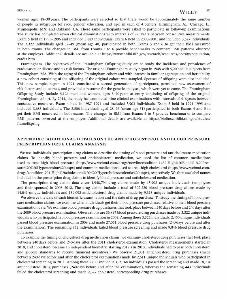
APPENDIX C : ADDITIONAL DETAILS ON THE ANTICHOLESTEROL AND BLOOD PRESSUREPRESCRIPTION DRUG CLAIMS ANALYSIS

We use individuals' prescription drug claims to describe the timing of blood pressure and anticholestero medicationclaims. To identify blood pressure and anticholesterol medication, we used the list of common medicationsused to treat high blood pressure (http://www.webmd.com/drugs/newlinecondition-1432-High%20Blood% %20Pres-sure%20%20Hypertension%20.aspx) and common medications used to treat high cholesterol (http://www.webmd.com/drugs/condition-701-High%20cholesterol%20%20 Hypercholesterolemia%20.aspx), respectively. We then use label namesincluded in the prescription drug claims to identify blood pressure and anticholesterol medication.

The prescription drug claims data cover 1,948,794 drug claims made by 45,903 unique individuals (employeesand their spouses) in 2008–2012. The drug claims include a total of 302,220 blood pressure drug claims made by14,041 unique individuals and 139,092 anticholesterol drug claims made by 9,313 unique individuals.

We observe the date of each biometric examination and the date of drug purchase. To study the timing of blood pres-sure medication claims, we examine when individuals get their blood pressure purchased relative to their blood pressureexamination date. We examine blood pressure drug purchases that took place between 240 days before and 240 days afterthe 2009 blood pressure examination. Observations are 36,897 blood pressure drug purchases made by 3,322 unique indi-viduals who participated in blood pressure examination in 2009. Among these 3,322 individuals, 2,450 unique individualspassed blood pressure examination in 2009 and made 27,051 blood pressure drug purchases (240 days before and afterthe examination). The remaining 872 individuals failed blood pressure screening and made 9,846 blood pressure drugpurchases.

To examine the timing of cholesterol drug medication claims, we examine cholesterol drug purchases that took placebetween 240 days before and 240 days after the 2011 cholesterol examination. Cholesterol measurements started in2010, and cholesterol became an independent biometric starting 2012. (In 2010, individuals had to pass both cholesteroland glucose standards to receive financial incentives.) We observe 21,031 anticholesterol drug purchases (madebetween 240 days before and after the cholesterol examination) made by 2,611 unique individuals who participated incholesterol screening in 2011. Among these 2,611 individuals, 2,168 individuals passed the screening and made 18,704anticholesterol drug purchases (240 days before and after the examination), whereas the remaining 443 individualsfailed the cholesterol screening and made 2,327 cholesterol corresponding drug purchases.

278 EINAV ET AL.

APPENDIX D : ADDITIONAL TABLES AND FIGURE

FIGURE D1 Relationship between body mass index (BMI) and health expenditure. Figure plots predictions from kernel regression oflog(yearly medical expenditure + 1) on BMI, separately for men and women. The dashed lines show the 95% confidence intervals, and thevertical dotted line shows the employer's passing standard (of 30). Observations are individual years in the complete data sample forindividuals who got their BMI measured. BMI measurements are missing for some individuals who auto-passed by passing all five metrics bysatisfying National Institutes of Health standards in the previous year or received an exemption (e.g., due to pregnancy). We droppedobservations with BMI below the 0.5th percentile and above 99.5th percentiles. The sample includes 55,373 individual-year observations,consisting of 10,892 unique men individuals and 12,670 unique women

TABLE D1 Comparisons with Coronary Artery Risk Development in Young Adults (CARDIA) and Framingham, adjusting forage and gender

Matching method Treated Controls Difference Standard error t statistics

Outcome variable: Change in BMICARDIA Unmatched 0.113 1.272 −1.159 0.05 − 21.83

Kernel 0.151 0.905 −0.754 0.53 −1.421-Nearest-neighbor 0.113 0.735 −0.622 1.24 −0.505-Nearest-neighbor 0.113 0.841 −0.728 0.65 −1.12

Framingham Unmatched 0.113 0.620 −0.507 0.05 − 10.37Kernel 0.113 0.742 −0.629 0.05 − 12.071-Nearest-neighbor 0.113 0.526 −0.413 0.24 −1.745-Nearest-neighbor 0.113 0.545 −0.432 0.12 −3.49

“Treatment” refers to workplace wellness program participants, and “control” refers to CARDIA or Framingham participants. We use logit regressionand regress treatment on age and gender to estimate the propensity scores. For kernel matching, we use the Epanechnikov kernel and 0.06 bandwidth.Once individuals are matched, we can compare change in body mass index between workplace participants and CARDIA/Framingham participants.This is an estimate of the “average treatment effect on the treated.” For the top panel, observations include 6,845 workplace wellness program participantsand 3,322 CARDIA participants. For the bottom panel, observations include 6,845 workplace wellness program participants and 3,506 Framinghamparticipants.a For workplace wellness program participants, 4,631 are on support, and 2,214 are off support.

EINAV ET AL. 279

TABLE D2 Results form a two-part model

Depedent variable: Log(medical expenditure + 1)logit GLM logit GLM logit GLM logit GLM logit GLM

A. MalesBMI 0.0451 0.00434

(0.0036) (0.00033)BP (systolic) −0.0041 −0.00002

(0.0014) (0.00013)BP (diastolic) −0.0037 −0.00039

(0.0019) (0.00019)Cholesterol −0.005 −0.00036

(0.0005) (0.00005)Glucose 0.0042 0.00048

(0.0013) (0.00010)N (individual years) 25,768 25,768 25,845 25,845 25,821 25,821 18,630 18,630 17,893 17,893N (unique individuals) 10,892 10,892 10,914 10,914 10,904 10,904 9,033 9,033 8,869 8,869B. FemalesBMI 0.0114 0.00239

(0.0035) (0.00020)BP (systolic) −0.0079 −0.00006

(0.0017) (0.00010)BP (diastolic) −0.0047 −0.00017

(0.0024) (0.00014)Cholesterol −0.0021 −0.00007

(0.0007) (0.00004)Glucose 0.0003 0.00029

(0.0017) (0.00010)N (individual years) 29,605 29,605 30,129 30,129 30,088 30,088 21,863 21,863 21,352 21,352N (unique individuals) 12,670 12,670 12,823 12,823 12,814 12,814 10,879 10,879 10,785 10,785

Note. BMI: body mass index; BP: blood pressure; GLM: generalized linear model. Table reports coefficients and standard errors (in parentheses) from atwo-part model regressing log(annual medical expenditure + 1) on each biometric measure separately. A logit model is fit for the probability of observing apositive-versus-zero outcome. Then, conditional on a positive outcome, a GLM model is fit for the positive outcome. Observations are individual years in the“complete data” sample restricted to individuals who got their biometrics measured. Biometric measurements are missing for some individuals who auto-passedby passing all five metrics by satisfying National Institutes of Health standards in the previous year or received exemptions. For each biometric, we dropped obser-vations below the 0.5th percentile and above 99.5th percentiles. Cholesterol and glucose measurement started in 2010 only. In addition to the reported coefficient,each regression includes year fixed effects and individual age fixed effects.

TABLE D3 Heterogeneity in the relationship between health changes and spending changes

Dependent variable: Log(medical expenditure + 1)Split by maximum expenditure Split by maximum BMIBelow median Above median BMI≤ 30 BMI> 30

BMI 0.0157 0.0197** 0.0144 0.0236*(0.0121) (0.00929) (0.00892) (0.0129)

N (individual years) 27,637 27,736 44,040 11,333N (unique individuals) 13,022 10,540 18,204 5,358

Note. BMI: body mass index. Table reports the same specification as in Table 5 of the main text but splitsindividuals based on their spending levels (left two columns) and BMI levels (right two columns). To cre-ate the split, we generate the highest annual spending (or BMI) of an individual that is observed over theentire observation period and use this highest level to define individual as above or below the median highestspending or above and below a highest BMI of 30.