The Impact of Differential Payroll Tax Subsidies on Minimum Wage Employment

1

The Impact of Differential Payroll Tax Subsidieson Minimum Wage Employment

Francis Kramarz, CREST- INSEE, CNRS, CEPR, and IZAThomas Philippon, MIT

September 2000

The authors would like to thank two anonymous referees as well as David Card, Bart Cockx, Bruno Crépon,Jennifer Hunt, Steve Machin, Thomas Piketty, Paolo Sestito Bruce Shearer for very helpful comments andsuggestions. We would also like to thank participants at the CEPR-Brussels Conference on minimum wage, theCNRS winter workshop in Aussois, and at the CREST, Hebrew University in Jerusalem, IZA, LSE, University ofBonn, UCL, and University of Toulouse-IDEI seminars for their remarks on previous versions of this paper.Corresponding author : Francis Kramarz, Crest-Insee, 15 bd Gabriel Péri, 92245 Malakoff, France, e-mail :[email protected] data were taken from the “Enquête Emploi” research files constructed by the Institut National de laStatistique et des Etudes Economiques (INSEE, the French national statistical agency). For further informationcontact: INSEE, Département de la diffusion, 18 bd Adolphe Pinard, 75675 Paris Cedex 14, France.

2

The Impact of Differential Payroll Tax Subsidies

on Minimum Wage Employment

Abstract

In this article, we study the impact of changes of total labor costs on employment of low-wage workersin France in a period, 1990 to 1998, that saw sudden and large changes in these costs. We uselongitudinal data from the French Labor Force survey (« enquête emploi ») in order to understand theconsequences of real decreases and real increases of the labor cost. We examine the transitionprobabilities from employment to non-employment and from non-employment to employment. Inparticular, we compare the transition probabilities of the workers that were directly affected by thechanges (“between” workers) with the transition probabilities of workers closest in the wage distributionto those directly affected (“marginal” workers). In all years with an increasing minimum cost, the“between” group (or the treated using the vocabulary of controlled experiments) comprises all workerswhose costs in year t lie between the old (year t) and the new (year t+1) minimum. In all years with adecreasing minimum, the “between” group comprises all workers whose costs in year t+1 lie betweenthe present minimum cost (year t+1) and the old (year t) minimum cost. The results can be summarizedas follows. Comparing years of increasing minimum cost and decreasing minimum cost, difference-in-difference estimates imply that an increase of 1% of the cost implies roughly an increase of 1.5% in theprobability of transiting from employment to non-employment for the treated workers, the resultingelasticity being –1.5. Second, results for the transitions from non-employment to employment are lessclear-cut. Tax subsidies have a small and insignificant impact on entry from non-employment as well ason transitions within the wage distribution. Finally, we show that the “marginal” group constitutes agood control group. In addition, there is no obvious evidence of substitution between the “between” and“marginal” groups of workers, but there is some evidence of substitution between workers within the taxsubsidy zone, with wages above those of the “marginal”, and workers outside the subsidy zone.

Keywords: Minimum Wage, Total Labor Costs, Tax SubsidiesJEL Classifications: J31, J23

Francis Kramarz Thomas PhilipponCREST-INSEE and CEPR MITDépartement de la Recherche Department of Economics15, bd Gabriel Péri 50, Memorial Drive92245 Malakoff Cedex. Cambridge, MA, 02142-1347France [email protected] [email protected]

3

1. Introduction

The importance of minimum wages on labor market outcomes is a matter of considerabledebate. Some argue that minimum wage changes have no visible impact on employment (see thediscussions surrounding the Card and Krueger’, 1994 study; see also Card and Krueger, 1998and Card and Krueger, 1995 for a recent critical analysis of the literature; see also Dickens,Machin, and Manning, 1998 for an analysis of the UK). While some others find that the fallingreal minimum wage over the eighties had impacts both on the employment of young as well asadult workers, and on the increase in wage inequality in the U.S. (see Brown, Gilroy, and Kohen,1982 for the classic survey of the employment effects of minimum wages; Brown, 1999 for anew comprehensive survey; Dolado, Kramarz, Machin, Manning, Margolis, and Teulings, 1996for a European perspective; Neumark and Washer, 1992 for the US, Abowd, Kramarz, Lemieux,and Margolis, 2000 for young workers or Abowd, Kramarz, and Margolis, 1999 for adultworkers both in France and in the US; and DiNardo, Fortin, and Lemieux, 1996, and Lee, 1999for inequality).

All these studies, indeed almost all existing ones, use wages as a measure of total labor costs.While this is a good measure for the low-wage labor market in the U.S. it is far from beingadequate in Continental Europe. Indeed, in France, for a worker paid at the minimum wage,employee-paid contributions increased from 12.22% of the wage in 1980 to 20.02% at thebeginning of 1993 whereas employer-paid contributions remained roughly stable (from 39.00%to 39.19%). But, starting in 1993, the employer-paid contributions started to decrease forminimum-wage workers (from 36.49% of the wage in 1993 to 21.77% in 1996), even though theminimum wage increased steadily over this period. Furthermore, the subsidies increaseddramatically and, maybe, unexpectedly, between 1995 and 1996.

In this article, we study the impact of changes of total labor costs on employment of low-wageworkers in France in a period, 1990 to 1998, that saw steady increases followed by sudden andlarge decreases in minimum costs. The tax subsidies were expected to counteract the negativeimpact of high minimum costs in a country with a large unemployment rate, in particular foryoung and uneducated workers.

We use longitudinal data from the French Labor Force survey (« enquête emploi ») in order tounderstand the consequences of real decreases and real increases of the labor cost. We examinethe transition probabilities from employment to non-employment and from non-employment toemployment. To estimate the effects of the changing cost, we compare these transitions betweenyears as well as within a year. In particular, we compare the transition probabilities of theworkers that were directly affected by the changes, the “between” workers, with the transitionprobabilities of workers closest in the wage distribution to those directly affected, the “marginal”workers. In all years with an increasing minimum cost, the “between” group (the treated usingthe vocabulary of controlled experiments) comprises all workers whose costs in year t liebetween the old (year t) and the new (year t+1) minimum. In those years, we examine whetherthese workers lose employment more frequently than workers paid marginally above the newminimum cost (the control group). In all years with a decreasing minimum, the “between” groupcomprises all workers whose costs in year t+1 lie between the present minimum cost (year t+1)

4

and the old (year t) minimum cost. In those years, we examine whether such workers come moreoften from non-employment than those paid marginally above the old minimum cost (the“marginal” group). We complement the first (simple difference) estimates with a difference-in-difference analysis in which the gap in employment to non-employment transitions between thetreated group and the control group, in years of increasing minimum costs, is compared to thesame gap in years of decreasing minimum costs. Similarly, we compare the gap in non-employment to employment transitions between the “between” group and the “marginal” groupin years of decreasing minimum costs with the one observed in years of increasing minimumcosts. If employment transitions of the “between” group differ structurally from those of the“marginal” group, the difference-in-difference analysis eliminates these unobserved components.

The results can be summarized as follows. Comparing years of increasing minimum cost anddecreasing minimum cost, difference-in-difference estimates imply that an increase in cost of1% implies roughly an increase of 1.5% in the probability of transiting from employment tonon-employment for the treated workers, the resulting elasticity being –1.5. There is strongevidence that the effects of cost increases and cost decreases are not symmetric.Unfortunately, the results for the transitions from non-employment to employment are lessclear-cut. Even though tax subsidies seem to have an impact on entry from non-employment,this effect is not significantly different from zero. We also show that the “marginal” group ofworkers constitute a good control group in our difference-in-difference analysis. Finally, taxsubsidies appear to have an effect on transitions within the wage distribution.

In the next section, we present the legal framework surrounding the changes in the minimumwage and in the payroll taxes and their impact of the cost of workers paid around theminimum wage. In Section 3, we present the data that we use as well as first descriptiveevidence. In Section 4, we specify our statistical models; the resulting estimates beingpresented and discussed in Section 5. We briefly conclude in Section 6.

2. Legal Framework

The first minimum wage law in France was enacted in 1950, creating a guaranteed hourly wagerate that was partially indexed to the rate of increase in consumer prices. Beginning in 1970, theoriginal minimum wage law was replaced by the current system (called the SMIC, “salaireminimum interprofessionnel de croissance”) linking the changes in the minimum wage to bothconsumer price inflation and growth in the average hourly blue-collar wage rate. In addition toformula-based increases in the SMIC, the government legislated increases many times over thenext two decades (the so-called “coup de pouce”). The statutory minimum wage in Franceregulates the hourly regular cash compensation received by an employee, including theemployee’s part of any payroll taxes.1

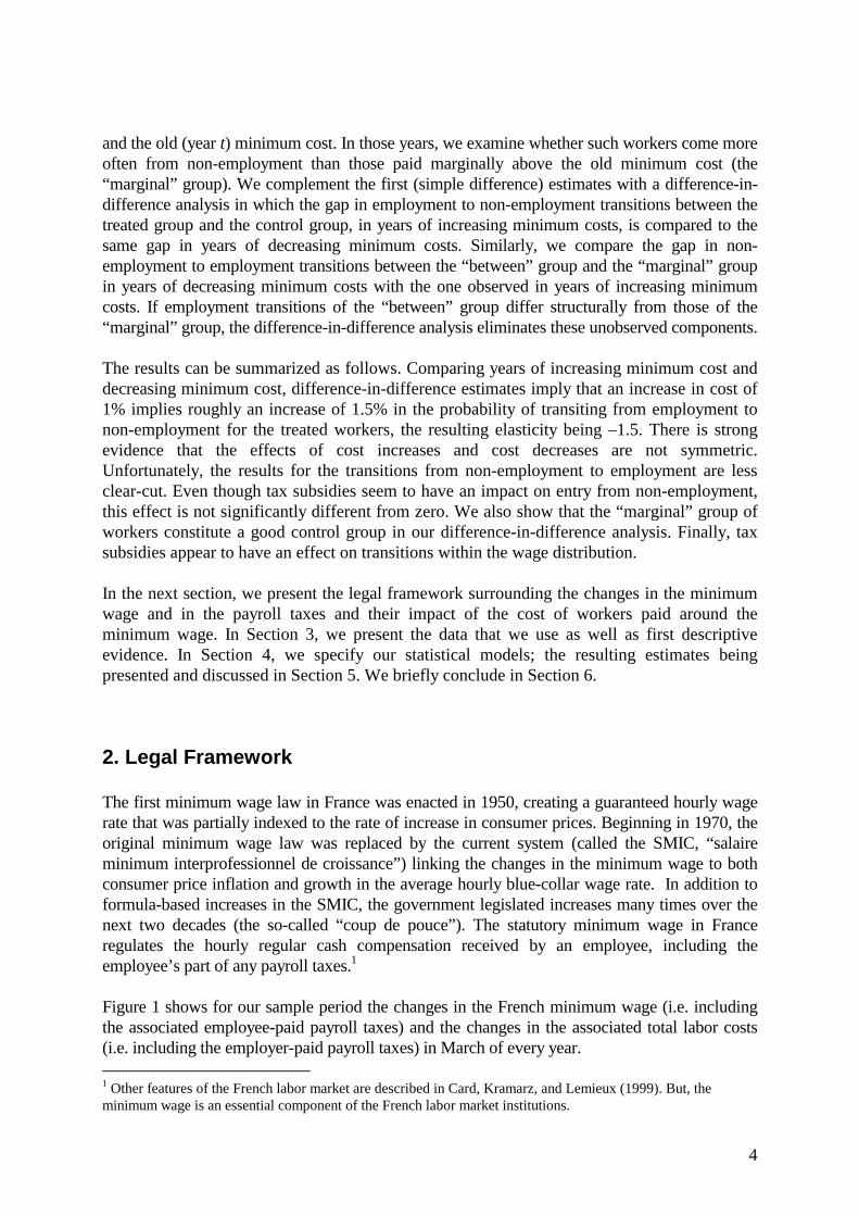
Figure 1 shows for our sample period the changes in the French minimum wage (i.e. includingthe associated employee-paid payroll taxes) and the changes in the associated total labor costs(i.e. including the employer-paid payroll taxes) in March of every year. 1 Other features of the French labor market are described in Card, Kramarz, and Lemieux (1999). But, theminimum wage is an essential component of the French labor market institutions.

5

Figure 1: Changes in the Real Minimum Cost and the Real Minimum WageSources: Dares (various years), Insee (various years)

Because of the extensive use of payroll taxes to finance mandatory employee benefits, theFrench minimum wage imposed a substantially greater cost upon the employer than its statutoryvalue. In addition, the real (statutory) minimum wage increased over the whole period, partlybecause of increases in the employee-paid payroll taxes, partly because of the voluntary policy ofthe various French governments. To counteract this increasing burden, tax exemptions wereenacted during this period. Figure 2 presents the various policies that were successivelyimplemented over the nineties. The year refers to the situation in March, the month of the Frenchlabor force survey, the data that we use in the following. In March 1994, the subsidy is made oftwo flat rates, the first one, ranging from 1 to 1.1 times the minimum wage, is equal to 5.4%,while the second, ranging from 1.1 to 1.2 times the minimum wage, is equal to 2.7%. In 1995,

0

1000

2000

3000

4000

5000

6000

7000

8000

90 91 92 93 94 95 96 97 98

year

real

fran

cs

real minimum costreal gross minimum wage

6

the ranges became respectively 1-1.2 and 1.2-1.3. In September 1995 (dated 1996 in Figure 2),the subsidy increased dramatically and its shape changed, decreasing from 18% to 5.4% forwages going from 1 times the minimum wage to 1.2 times the minimum wage. In October 1996(dated 1997 in Figure 2), the two subsidies were merged in one linear reduction that spannedfrom 1 to 1.33 times the minimum wage. In 1998, the subsidy did not change.

Figure 2: The Tax Subsidies, 1994 to 1998

Hence, between 1993 and 1995, the tax reductions were rather small (at most 6% for a minimumwage worker). But, starting in September 1995, reductions became substantial and the employer-payroll taxes decreased by 18 percentage points at the minimum wage. Employer-paid payrolltaxes went from roughly 40% at the beginning of the nineties to 21.77% in 1996. The nextfigures show the impact of the subsidies on the changes of costs for workers with a wagebetween the minimum wage and twice the minimum wage for the various years of our sample.

Reduction of Employer-Paid Payroll Taxes

0

2

4

6

8

10

12

14

16

18

20

1 1,05 1,1 1,15 1,2 1,25 1,3 1,35

Gross Wage/Min. Wage

% R

educ

tion/

Gro

ss W

age

19941995199619971998

7

Cha

nge

in C

osts

Figure 3a: Changes in Costs, 1990-1991Ratio of Cost/Minimum Cost

1 2

0

474.301

Cha

nge

in C

osts

Figure 3b: Changes in Costs, 1991-1992Ratio of Cost/Minimum Cost

1 2

0

206.181

Cha

nge

in C

osts

Figure 3c: Changes in Costs, 1992-1993Ratio of Cost/Minimum Cost

1 2

0

86.627

8

Cha

nge

in C

osts

Figure 3d: Changes in Costs, 1993-1994Ratio of Cost/Minimum Cost

1 2

-348.245

0

Cha

nge

in C

osts

Figure 3e: Changes in Costs, 1994-1995Ratio of Cost/Minimum Cost

1 2

-384.883

94.5308

Cha

nge

in C

osts

Figure 3f: Changes in Costs, 1995-1996Ratio of Cost/Minimum Cost

1 2

-764.147

0

9

Cha

nge

in C

osts

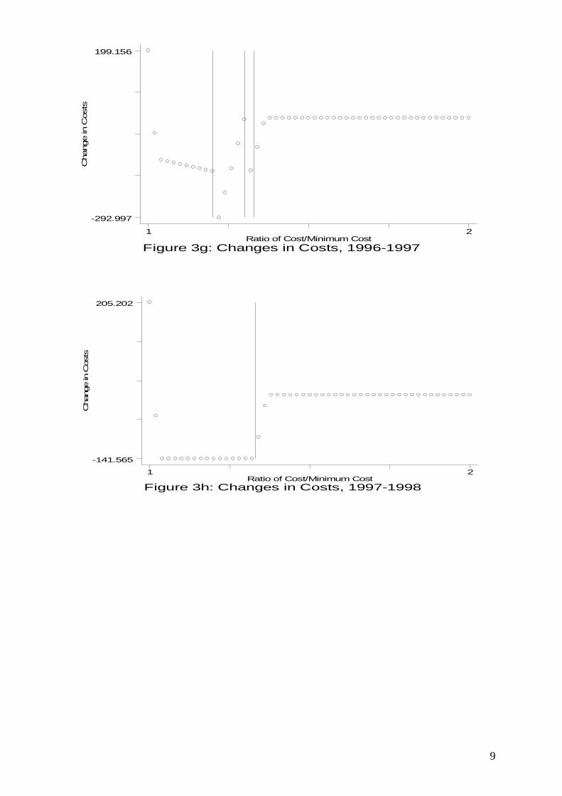
Figure 3g: Changes in Costs, 1996-1997Ratio of Cost/Minimum Cost

1 2

-292.997

199.156

Cha

nge

in C

osts

Figure 3h: Changes in Costs, 1997-1998Ratio of Cost/Minimum Cost

1 2

-141.565

205.202

10

In Figures 3a to 3h, we have computed the changes in nominal costs between consecutive yearsinduced by changes in the minimum wage and subsidies of each year.2 To simplify our thedescriptive analysis, we do not show changes in costs induced by other changes in the tax system(such as health, or pensions), even though we compute and use the exact changes in the rest ofthe analysis. More precisely, we assume for this computation that workers paid w at the initialdate will be paid exactly w at the next date unless the old wage is between the old and the newminimum wage. If we consider the first three couples of years (Figures 3a to 3c), we see thatchanges are solely due to increases in the minimum wage. Workers at the minimum have thelargest change, whereas workers with a wage above the new nominal minimum wage have anunchanged cost (given the assumptions used for this descriptive analysis). Starting in 1993-1994,the subsidies interact with the changes in the minimum wage. The vertical lines reflect theschedule of the subsidies (at 1.1, 1.2, 1.3, and 1.33 times the minimum wage depending on theyear). For instance, changes between 1993 and 1994 are characterized by a small increase in theSMIC, a decrease in payroll taxes for workers with wage between the SMIC and 1.1 times theSMIC, and a smaller decrease between 1.1 and 1.2 times the minimum wage. All workers with awage in 1993 above 1.2 times the new minimum are unaffected by these changes. The largestdecrease occurs between 1995 and 1996 when the employer payroll taxes decrease by 18.2percentage points, inducing a decrease in costs of more than 700 French Francs (120 US$) forworkers close to the minimum. Finally, Figure 3h displays a very particular and interestingfeature induced by the interaction of a large increase in the minimum wage and subsidies basedon the same minimum wage. The minimum wage strongly increased after Jacques Chirac’selection as president (a tradition in France after every presidential election). Hence, workers thatwere above the minimum wage in 1997, say at 1.1 times the minimum, had a wage at theminimum in 1998. Subsidies for such workers increased, say from 10 percentage points to themaximum of 18.2 percentage points. Consequently, their cost decreased. Therefore, theminimum wage increase induced a decrease in the cost of workers who had, in 1997, a wagebetween the new minimum wage and 1.33 times the old minimum. We will use the structure ofthese various changes in our econometric analysis. Notice, however, that the variousdiscontinuities that show up on the figures are, in reality, smoothed by the changes in the rates ofother taxes, such as those paying for the health-care system or for pensions.

In addition to these reductions for low-wage workers, contracts in various youth employmentprograms offer either minimum wage exemptions (apprenticeship, for instance) or payroll taxexemptions. These programs were the focus of Bonnal, Fougère, and Sérandon (1997) and ofMagnac (1997). To fully concentrate on the effects of the changes in the labor cost for the usualtypes of contracts, we will not include young workers (below 25) employed under any specialprogram in our analysis. Indeed, they only represent a very small proportion of the employedpopulation.

2 As in the previous Figures, the computations reflect the situation as of March of the year.

11

3. Data and First Evidence

3.1. Data Description

The data were extracted from the French «Enquête Emploi» (Labor Force Survey) for the years1990 to 1998. The sixty thousand households included in the Labor Force Survey sample areinterviewed in March of three consecutive years with one-third of the households replaced eachyear. Every member of the household is surveyed and followed provided that he or she does notmove during this three-year period. We used the INSEE research files for each of the indicatedyears. These files include the identifiers that allow us to follow individuals from year to year.Using these identifiers we created year-to-year matched files for the years 1990-91 to 1997-98.

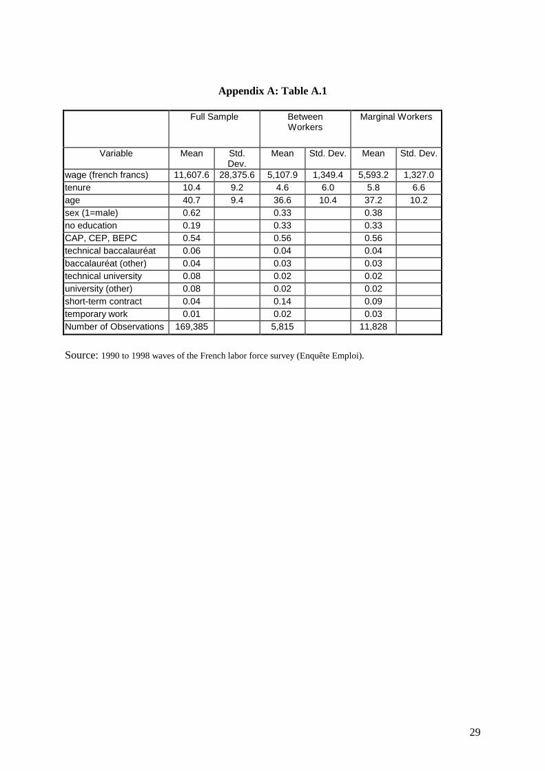
The survey measures usual monthly earnings, net of employee payroll taxes but includingemployee income taxes, and usual weekly hours. The minimum wage is defined on an hourlybasis, unfortunately the usual weekly hours measure appears to be somewhat noisy. A lot ofrespondents say that they work more than 39 hours per week, the legal limit. If one calculates anhourly wage, an unreasonable fraction is paid below the minimum. For instance, some high-paidyoung engineers declare more than 50 hours a week. Therefore, we used the monthly wagetogether with the full-time or part-time status to compute the total labor cost. For workersemployed part-time, we used the reported weekly hours to compute their full-time equivalentmonthly wage. For full-time workers, we use the reported monthly wage.All young workers employed in publicly-funded programs that either combined classroomeducation with work («apprentis», «stage de qualification» or «stage d’insertion, contrat emploi -formation») or provide subsidized low-wage employment (such as «SIVP, stage d’initiation à lavie professionnelle» ) were excluded from the database. All of these programs provide a legalexemption from the SMIC and from certain payroll taxes. These programs are limited to workers25 years old and under. In addition, all workers who declared a wage below 95% of theminimum wage without reporting employment on a special scheme were not kept in the analysisfile (they represent less than 5% of the original file). Most correspond to reporting or codingerrors as well as workers on special contracts who did not specify the type of contract. We alsoeliminated workers employed as civil-servants or in the public sector since they cannot becomenon-employed, owing to their status.The employment status in year t is equal to one for all individuals who are employed in March ofthe survey year, and equal to 0 otherwise. The French Labor Force Survey definition ofemployment is the same as the one used by the International Labor Office: a person is employedif he or she worked for pay for at least one hour during the reference week. The definition isthus consistent with the American BLS definition.Our control variables consist of education, age, sex, seniority, type of contract, wage, and year.Education was constructed as six categories: none; completed elementary school, junior highschool, or basic vocational/technical school; completed advanced vocational/technical school;completed high school (baccalauréat); completed technical college; completed undergraduate orgraduate university. Seniority was measured as the response to a direct question in the survey(years with the present employer). The type of contract was constructed as 3 categories: short-term contracts (CDD), temporary work, long-term contracts (CDI). Summary statistics arepresented in Table A.1 in the Data Appendix.

12

The data on minimum wage, price index and taxes were taken from « Les Retrospectives »,BMS ( Bulletin Mensuel de Statistiques, INSEE) in March of each year. The data on taxsubsidies were taken from « Liaisons Sociales » (DARES) and « Séries longues sur lesSalaires » ( INSEE Résultats, édition 1998).

3.2. Descriptive Analysis

Figure 4a presents a non-parametric estimation of the probabilities of being non-employed atdate t+1 conditional on being employed at date t as a function of the ratio of the cost to theminimum cost for two couples of years, 1990-1991 and 1995-1996. These years were selectedbecause the GDP growth rates were similar, but with an increasing minimum cost for the firstcouple of years and a decreasing minimum cost for the second couple of years.

In particular, in every year, workers with higher wages are less likely to become non-employed.The vertical lines correspond, from the left to the right to 0.98, 1.03, 1.1, 1.2, and 1.3 times theminimum wage. Our “between” workers (our treated group) are roughly comprised between thefirst two lines, the “marginal” workers (our control group) are roughly comprised between thesecond and the third, whereas the last two lines correspond to the steps in the subsidy schedulethat prevails in 1996. Considering first the 1990-1991 transitions, the “between” workers, i.e.those directly concerned by the minimum wage increase, have a higher job loss probability than

Figure 4a: Job Losses, 1990-91 and 1995-96, w.r.t the SMICratio of wage/minimum wage

Job Loss Prob. 90-91 Job Loss Prob. 95-96

.95904 1.99843

.031982

.153525

0.981.03 1.10 1.20 1.30

13

the “marginal” workers, who also have a higher job loss probability than the rest of thedistribution. Notice also that “marginal” workers have a roughly constant job loss probabilitywhereas “between” workers’ mirrors the minimum cost increase shown in Figure 3a. The 1995-1996 job loss probability distribution has changed, in particular in the tax subsidy zone, wherethe subsidy is the largest, i.e. close to the minimum wage, where the job loss probabilitydecreases. Indeed, the changes do not seem much stronger for the “between” than for the“marginal” workers. In fact, comparing the two couples of years in Figure 4a, there is no obviousevidence of substitution between “marginal” and “between” workers. Indeed, from this figure,effect of the changes in minimum cost between the two couples of years may appear to bedifficult to isolate. An estimation controlling for all observed factors is needed.

Simultaneously, the decrease in the minimum cost may have favored entry of low-wage workers.Therefore, we contrast entries over the same two couples of years. Figure 4b presents non-parametric estimates of the probability of coming from non-employment (in 1990 and 1995,respectively) for workers employed in the next year (1991 and 1996, respectively) as a functionof the ratio of the wage to the minimum wage. Once again, the vertical lines correspond, fromthe left to the right to 0.98, 1.03, 1.1, 1.2, and 1.3 times the minimum wage.

The results do not show any obvious difference between the two couples of years, even thoughmore entry seems to take place in the bottom of the wage distribution in all years. Indeed,

Figure 4b: Job Entry, 1990-91 and 1995-96, w.r.t the SMICratio of wage/minimum wage

Job Entry Prob. 90-91 Job Entry Prob. 95-96

.95904 1.99843

.027984

.201653

0.98 1.03 1.10 1.20 1.30

14

business conditions were not exactly similar in those two couples of years even though theywere close. This may explain the slightly larger entry in 1990-1991. Notice that “marginalworkers” do not seem to benefit from the decrease in costs more than “between workers”. Moredetailed statistical analysis is obviously needed here and will be presented in the next sections.Just note that the “marginal” workers, that we use as a control group in our statistical analysis,do not seem to be affected by substitution. But, we will come back to this question later in theanalysis. We now turn to our statistical framework in order to analyze the effects of thechanges in the minimum costs more systematically.

4. The Statistical Models

Our first interest is the analysis of the impact of minimum wage increases on transitions tonon-employment of workers directly affected by the increase. Therefore, we isolate theseworkers in our statistical framework. From the Figures 3a to 3h presented above, we see thatyears 1990 to 1992 are excellent examples of years in which the cost for minimum workersincreases while that of workers just above the new minimum does not change. The largeminimum wage increase that occurs between 1997 and 1998 is also an example whereworkers at the minimum are directly affected even though tax subsidies were already in place.In fact, workers above the new minimum up to 1.33 times the old minimum benefited from adecrease in costs. But, importantly for us, workers just above the new minimum, say betweenthe new minimum and 1.1 times the new minimum benefit from the same decrease as workerswith wage between 1.1 and 1.3 times the new minimum. Hence, in our period analysis,minimum costs increased by much larger factor than for all other categories of workers. Theeffects of such increases can be contrasted with the effects of decreases in costs that occurredduring the same period. In particular, the above Figures show that two couples of years, 1995-1996 and 1993-1994, are undoubtedly years of decreasing cost for minimum wage workers.Furthermore, in those two couples of years, workers situated above in the wage distributionbenefited less from the tax subsidies than minimum wage workers.

Therefore, our statistical analyses will contrast outcomes of workers most affected by thechanges – increases in the minimum wage or decreases in the minimum costs afterimplementation of tax subsidies - with those closest to them in the wage distribution but eithernot affected or less affected by the changes.

A look at the same Figures might lead us to use some of the discontinuities that appear in thechanging costs (the statistical methods well-suited to using such discontinuities for programevaluation are presented in Angrist and Lavy, 1999, van der Klaauw, 1996; they are based onideas of Campbell, 1969). However, there are at least two reasons for not using this type ofapproach in our particular application. First, the Figures show changes that are not the onlycost changes that occur in any given year. In particular, our computations of cost changesinclude other component of the taxes that are not shown on the graphs but are used in ourstatistical analysis. As already mentioned, these other components tend to smooth the changes.Furthermore, the data on wages that we use is not precise enough to locate and examineprecisely the discontinuities. These wages come from a household survey, and manycomponents of the wage cannot be isolated. For instance, a precise measure of the bonuses isessential to assess the exact situation of a worker vis-à-vis the minimum wage and, therefore,

15

vis-à-vis tax subsidies when the wage is around 1.2 or 1.3 times the minimum. Suchinformation is not available in the French enquête emploi. Administrative data sources wouldbe more suited to such analysis.

4.1. Exit

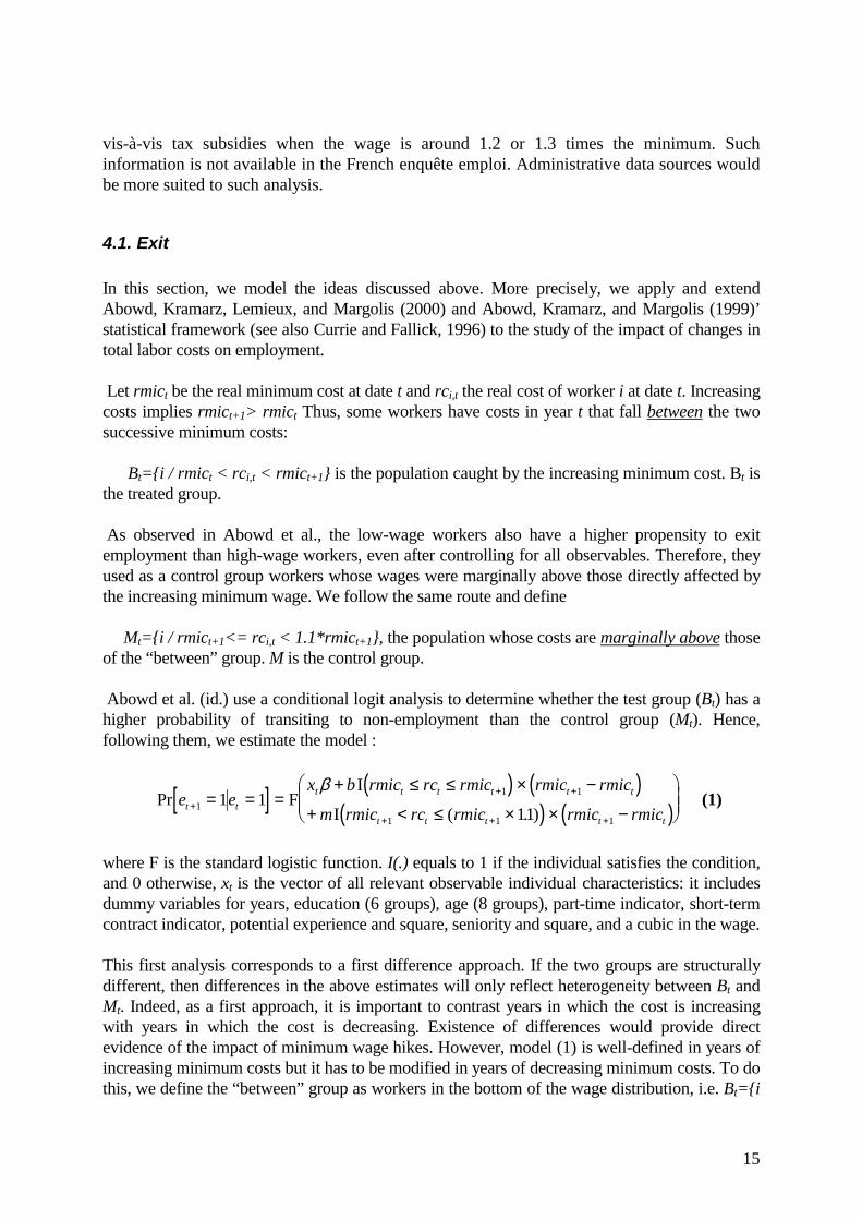
In this section, we model the ideas discussed above. More precisely, we apply and extendAbowd, Kramarz, Lemieux, and Margolis (2000) and Abowd, Kramarz, and Margolis (1999)’statistical framework (see also Currie and Fallick, 1996) to the study of the impact of changes intotal labor costs on employment.

Let rmict be the real minimum cost at date t and rci,t the real cost of worker i at date t. Increasingcosts implies rmict+1> rmict Thus, some workers have costs in year t that fall between the twosuccessive minimum costs:

Bt={i / rmict < rci,t < rmict+1} is the population caught by the increasing minimum cost. Bt isthe treated group.

As observed in Abowd et al., the low-wage workers also have a higher propensity to exitemployment than high-wage workers, even after controlling for all observables. Therefore, theyused as a control group workers whose wages were marginally above those directly affected bythe increasing minimum wage. We follow the same route and define

Mt={i / rmict+1<= rci,t < 1.1*rmict+1}, the population whose costs are marginally above thoseof the “between” group. M is the control group.

Abowd et al. (id.) use a conditional logit analysis to determine whether the test group (Bt) has ahigher probability of transiting to non-employment than the control group (Mt). Hence,following them, we estimate the model :

[ ] ( ) ( )( ) ( )

Pr FI

I ( . )e e

x b rmic rc rmic rmic rmic

m rmic rc rmic rmic rmict tt t t t t t

t t t t t+

+ +

+ + +

= = =+ ≤ ≤ × −

+ < ≤ × × −

�

��

�

��1

1 1

1 1 1

1 111

β (1)

where F is the standard logistic function. I(.) equals to 1 if the individual satisfies the condition,and 0 otherwise, xt is the vector of all relevant observable individual characteristics: it includesdummy variables for years, education (6 groups), age (8 groups), part-time indicator, short-termcontract indicator, potential experience and square, seniority and square, and a cubic in the wage.

This first analysis corresponds to a first difference approach. If the two groups are structurallydifferent, then differences in the above estimates will only reflect heterogeneity between Bt andMt. Indeed, as a first approach, it is important to contrast years in which the cost is increasingwith years in which the cost is decreasing. Existence of differences would provide directevidence of the impact of minimum wage hikes. However, model (1) is well-defined in years ofincreasing minimum costs but it has to be modified in years of decreasing minimum costs. To dothis, we define the “between” group as workers in the bottom of the wage distribution, i.e. Bt={i

16

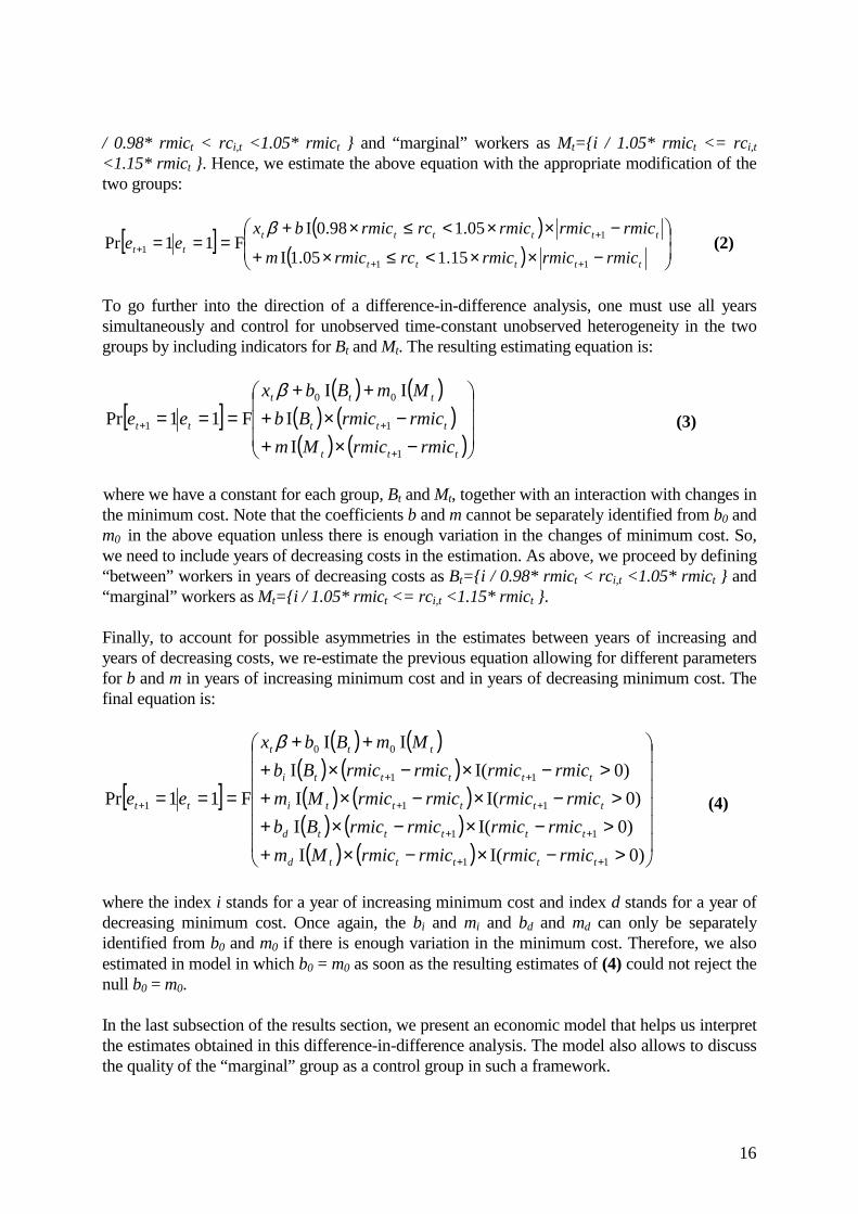
/ 0.98* rmict < rci,t <1.05* rmict } and “marginal” workers as Mt={i / 1.05* rmict <= rci,t<1.15* rmict }. Hence, we estimate the above equation with the appropriate modification of thetwo groups:

[ ] ( )( ) �

�

�

�

��

�

�

−××<≤×+

−××<≤×+===

++

++

ttttt

tttttttt rmicrmicrmicrcrmicm

rmicrmicrmicrcrmicbxee

11

11 15.105.1I

05.198.0IF11Pr

β (2)

To go further into the direction of a difference-in-difference analysis, one must use all yearssimultaneously and control for unobserved time-constant unobserved heterogeneity in the twogroups by including indicators for Bt and Mt. The resulting estimating equation is:

[ ]( ) ( )

( ) ( )( ) ( )�

��

�

�

��

�

�

−×+−×+

++===

+

++

ttt

ttt

ttt

tt

rmicrmicMmrmicrmicBbMmBbx

ee

1

1

00

1

II

IIF11Pr

β (3)

where we have a constant for each group, Bt and Mt, together with an interaction with changes inthe minimum cost. Note that the coefficients b and m cannot be separately identified from b0 andm0 in the above equation unless there is enough variation in the changes of minimum cost. So,we need to include years of decreasing costs in the estimation. As above, we proceed by defining“between” workers in years of decreasing costs as Bt={i / 0.98* rmict < rci,t <1.05* rmict } and“marginal” workers as Mt={i / 1.05* rmict <= rci,t <1.15* rmict }.

Finally, to account for possible asymmetries in the estimates between years of increasing andyears of decreasing costs, we re-estimate the previous equation allowing for different parametersfor b and m in years of increasing minimum cost and in years of decreasing minimum cost. Thefinal equation is:

[ ]

( ) ( )( ) ( )( ) ( )( ) ( )( ) ( ) �

��

�

�

��

�

�

>−×−×+>−×−×+>−×−×+

>−×−×+++

===

++

++

++

++

+

)0I(I)0I(I)0I(I

)0I(III

F11Pr

11

11

11

11

00

1

tttttd

tttttd

ttttti

ttttti

ttt

tt

rmicrmicrmicrmicMmrmicrmicrmicrmicBb


MmBbx

ee

β

(4)

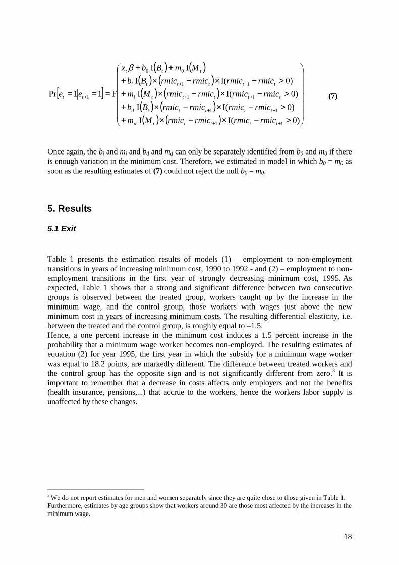
where the index i stands for a year of increasing minimum cost and index d stands for a year ofdecreasing minimum cost. Once again, the bi and mi and bd and md can only be separatelyidentified from b0 and m0 if there is enough variation in the minimum cost. Therefore, we alsoestimated in model in which b0 = m0 as soon as the resulting estimates of (4) could not reject thenull b0 = m0.

In the last subsection of the results section, we present an economic model that helps us interpretthe estimates obtained in this difference-in-difference analysis. The model also allows to discussthe quality of the “marginal” group as a control group in such a framework.

17

4.2. Entry

Decreasing cost implies rmict> rmict+1: thus, some workers have costs in year t+1 that arebetween the two successive minimum costs, Bt={i / rmict+1< rci,t+1 < rmict}. Hence, itconstitutes the population liberated by the decreasing minimum cost. Indeed, if workers arepaid their marginal product, this decrease in costs should allow non-employed workers toenter jobs. And, as above, we define Mt={i / rmict < rci,t+1 < rmict *1.1}, the population withcosts marginally above those of the “between” group.

As Abowd et al. (id.), we use a conditional logit analysis to determine whether the “between”group (B) has a higher probability of coming from non-employment than the “control” group(M).

Hence, we estimate the following model :

[ ] ( ) ( )( ) ( )��

��

�

−××≤<+−×≤≤+

===++

+++++

11

11111 )1.1(I

IF11Pr

ttttt

tttttttt rmicrmicrmicrcrmicm

rmicrmicrmicrcrmicbxee

β (5)

where all variables being defined as above.

Notice that the statistical framework is different in its interpretation from the previous onesince it adopts a retrospective perspective instead of a prospective one. In the classicevaluation problem, some workers receive a treatment and the statistician examines futureoutcomes. Here, we face the reverse situation since, in equation (5), we condition on output,i.e. the future location in the wage distribution to examine the past situation. In fact, this is anexample of the classic case-control studies in which the statistician examines what pastenvironment may have caused a future outcome, say what are the specific living conditions ofpersons affected by a particular disease. Prentice and Pyke (1979) show that the logisticframework that we use in our approach is adequate and that the interpretation of the resultingcoefficients in a retrospective study is similar to those obtained in a prospective study.

We will also estimate models equivalent to (2) and to the difference-in-difference equations(3) and (4), as explained for increasing costs, with the appropriate modifications:

[ ]( ) ( )

( ) ( )( ) ( )�

��

�

�

��

�

�

−×+−×+

++===

+

++

1

1

00

1

II

IIF11Pr

ttt

ttt

ttt

tt

rmicrmicMmrmicrmicBb

MmBbxee

β (6)

and

18

[ ]

( ) ( )( ) ( )( ) ( )( ) ( )( ) ( ) �

��

�

�

��

�

�

>−×−×+>−×−×+>−×−×+

>−×−×+++

===

++

++

++

++

+

)0I(I)0I(I)0I(I

)0I(III

F11Pr

11

11

11

11

00

1

tttttd

tttttd

ttttti

ttttti

ttt

tt



MmBbx

ee

β

(7)

Once again, the bi and mi and bd and md can only be separately identified from b0 and m0 if thereis enough variation in the minimum cost. Therefore, we estimated in model in which b0 = m0 assoon as the resulting estimates of (7) could not reject the null b0 = m0.

5. Results

5.1 Exit

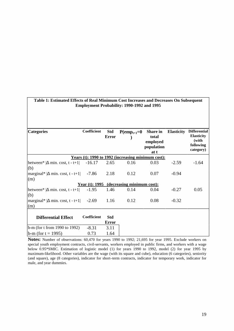
Table 1 presents the estimation results of models (1) – employment to non-employmenttransitions in years of increasing minimum cost, 1990 to 1992 - and (2) – employment to non-employment transitions in the first year of strongly decreasing minimum cost, 1995. Asexpected, Table 1 shows that a strong and significant difference between two consecutivegroups is observed between the treated group, workers caught up by the increase in theminimum wage, and the control group, those workers with wages just above the newminimum cost in years of increasing minimum costs. The resulting differential elasticity, i.e.between the treated and the control group, is roughly equal to –1.5.Hence, a one percent increase in the minimum cost induces a 1.5 percent increase in theprobability that a minimum wage worker becomes non-employed. The resulting estimates ofequation (2) for year 1995, the first year in which the subsidy for a minimum wage workerwas equal to 18.2 points, are markedly different. The difference between treated workers andthe control group has the opposite sign and is not significantly different from zero.3 It isimportant to remember that a decrease in costs affects only employers and not the benefits(health insurance, pensions,...) that accrue to the workers, hence the workers labor supply isunaffected by these changes.

3 We do not report estimates for men and women separately since they are quite close to those given in Table 1.Furthermore, estimates by age groups show that workers around 30 are those most affected by the increases in theminimum wage.

19

Table 1: Estimated Effects of Real Minimum Cost Increases and Decreases On SubsequentEmployment Probability: 1990-1992 and 1995

Categories Coefficient StdError

P(empt+1=0)

Share intotal

employedpopulation

at t

Elasticity DifferentialElasticity

(withfollowingcategory)

Years (t): 1990 to 1992 (increasing minimum cost):between* |∆ min. cost, t - t+1|(b)

-16.17 2.65 0.16 0.03 -2.59 -1.64

marginal* |∆ min. cost, t - t+1|(m)

-7.86 2.18 0.12 0.07 -0.94

Year (t): 1995 (decreasing minimum cost):between* |∆ min. cost, t - t+1|(b)

-1.95 1.46 0.14 0.04 -0.27 0.05


-2.69 1.16 0.12 0.08 -0.32

Differential Effect Coefficient StdError

b-m (for t from 1990 to 1992) -8.31 3.11b-m (for t = 1995) 0.73 1.64Notes: Number of observations: 60,470 for years 1990 to 1992; 21,695 for year 1995. Exclude workers onspecial youth employment contracts, civil-servants, workers employed in public firms, and workers with a wagebelow 0.95*SMIC. Estimation of logistic model (1) for years 1990 to 1992, model (2) for year 1995 bymaximum-likelihood. Other variables are the wage (with its square and cube), education (6 categories), seniority(and square), age (8 categories), indicator for short–term contracts, indicator for temporary work, indicator formale, and year dummies.

20

We conclude from this first analysis that there are strong differences between years ofincreasing and years of decreasing minimum costs. Workers caught up by the increase of theminimum wage tend to lose their job more often than “marginal” workers. However, there areways to go from these two simple difference analyses to a difference-in-difference analysis byestimating model (3) in which the effects are assumed to be symmetric. The estimates arepresented in Table 2.

Table 2: Estimated Effects of Real Minimum Cost Increases and Decreases On SubsequentEmployment Probability: Pooled Estimates


P(empt+1=0) Share intotal

employedpopulation

at t



Years (t): 1990 to 1992, 1997 (increasing min. cost), 1993, and 1995 (decreasing min.cost)between* (∆ min. cost, t - t+1)(b)

-2.31 1.13 0.15 0.03 -0.35 -0.38

marginal* (∆ min. cost, t - t+1)(m)

0.32 0.91 0.12 0.07 0.04


b-m (for t = 1990 to 1993, 1995,1997)

-2.63 1.37

Notes: Number of observations: 124,689 for years 1990 to 1993, 1995, and 1997. Estimation of model (3).Includes an indicator for the between group and an indicator for the marginal group. All other notes as in Table 1.

The difference-in-difference estimates of the effect of a 1% increase of the minimum cost, -0.38,are smaller than those presented in Table 1, but are still significantly different from zero.Remember that this model assumes that the effects of increases, years 1990 to 1992, and 1997and of decreases, years 1993, and 1995, in the minimum cost are symmetric.

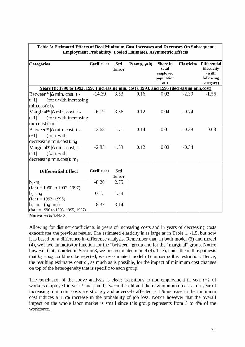
Table 3 presents the estimates of model (4) in which the symmetry is not assumed.

21

Table 3: Estimated Effects of Real Minimum Cost Increases and Decreases On SubsequentEmployment Probability: Pooled Estimates, Asymmetric Effects


P(empt+1=0) Share intotal

employedpopulation

at t



Years (t): 1990 to 1992, 1997 (increasing min. cost), 1993, and 1995 (decreasing min.cost)Between* |∆ min. cost, t -t+1| (for t with increasingmin.cost): bi

-14.39 3.53 0.16 0.02 -2.30 -1.56

Marginal* |∆ min. cost, t -t+1| (for t with increasingmin.cost): mi

-6.19 3.36 0.12 0.04 -0.74

Between* |∆ min. cost, t -t+1| (for t withdecreasing min.cost): bd

-2.68 1.71 0.14 0.01 -0.38 -0.03

Marginal* |∆ min. cost, t -t+1| (for t withdecreasing min.cost): md

-2.85 1.53 0.12 0.03 -0.34


bi -mi (for t = 1990 to 1992, 1997)

-8.20 2.75

bd -md (for t = 1993, 1995)

0.17 1.53

bi -mi - (bd -md)(for t = 1990 to 1993, 1995, 1997)

-8.37 3.14

Notes: As in Table 2.

Allowing for distinct coefficients in years of increasing costs and in years of decreasing costsexacerbates the previous results. The estimated elasticity is as large as in Table 1, -1.5, but nowit is based on a difference-in-difference analysis. Remember that, in both model (3) and model(4), we have an indicator function for the “between” group and for the “marginal” group. Noticehowever that, as noted in Section 3, we first estimated model (4). Then, since the null hypothesisthat b0 = m0 could not be rejected, we re-estimated model (4) imposing this restriction. Hence,the resulting estimates control, as much as is possible, for the impact of minimum cost changeson top of the heterogeneity that is specific to each group.

The conclusion of the above analysis is clear: transitions to non-employment in year t+1 ofworkers employed in year t and paid between the old and the new minimum costs in a year ofincreasing minimum costs are strongly and adversely affected; a 1% increase in the minimumcost induces a 1.5% increase in the probability of job loss. Notice however that the overallimpact on the whole labor market is small since this group represents from 3 to 4% of theworkforce.

22

5.2. Entry

Up to now, we have examined transitions from employment to non-employment. In thissubsection, we turn to the symmetric analysis: the impact of tax subsidies on the entry ofworkers. In particular, we want to see if workers who were previously unemployable – notproductive enough given the prevailing minimum cost – become employed after the decreasein the minimum cost.As a starting point, and similarly to the analysis of increasing costs, we estimate model (5) inyears of decreasing costs as well as in years of increasing costs. These first results arepresented in Table 4.

Table 4: Estimated Effects of Real Minimum Cost Decreases and Increases On PriorEmployment Probability: 1991-1993, 1994, 1996, and 1998


P(empt=0) Share intotal

employedpopulation

at t+1



Years (t+1): 1991 to 1993 (increasing minimum cost):between* |∆ min. cost, t - t+1|(b)

-7.44 2.61 0.19 0.04 -1.41 -0.92

marginal* |∆ min. cost, t –t+1| (m)

-3.26 2.26 0.15 0.08 -0.49

Year (t+1): 1994 (decreasing minimum cost):between* |∆ min. cost, t - t+1|(b)

-10.86 5.33 0.20 0.02 -2.17 -0.94


-7.70 3.70 0.16 0.07 -1.23

Year (t+1): 1996 (decreasing minimum cost):between* |∆ min. cost, t - t+1|(b)

-2.72 1.31 0.20 0.06 -0.54 -0.43


-0.91 1.52 0.13 0.05 -0.12

Years (t+1): 1998 (increasing minimum cost):between* |∆ min. cost, t - t+1|(b)

2.90 5.56 0.10 0.09 0.29 0.36


-0.85 5.50 0.08 0.09 -0.07


b-m (for t+1 from 1991 to 1993) -4.18 2.99b-m (for t+1 = 1994) -3.16 5.78b-m (for t+1 = 1996) -1.81 1.73b-m (for t+1 = 1998) 3.76 6.43Notes: Number of observations: 60,428 for years (t+1) 1991 to 1993; 21,465 for 1994; 21,707 for 1996; 16,379for 1998. All other notes as in Table 1.

23

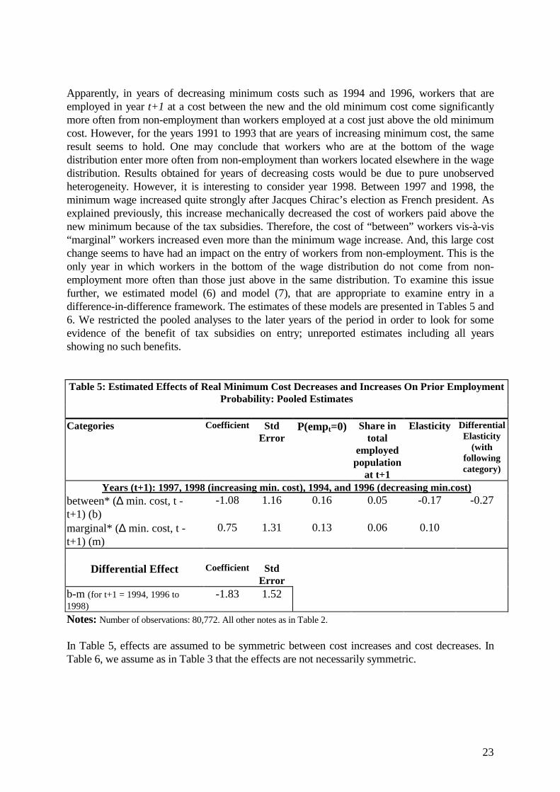
Apparently, in years of decreasing minimum costs such as 1994 and 1996, workers that areemployed in year t+1 at a cost between the new and the old minimum cost come significantlymore often from non-employment than workers employed at a cost just above the old minimumcost. However, for the years 1991 to 1993 that are years of increasing minimum cost, the sameresult seems to hold. One may conclude that workers who are at the bottom of the wagedistribution enter more often from non-employment than workers located elsewhere in the wagedistribution. Results obtained for years of decreasing costs would be due to pure unobservedheterogeneity. However, it is interesting to consider year 1998. Between 1997 and 1998, theminimum wage increased quite strongly after Jacques Chirac’s election as French president. Asexplained previously, this increase mechanically decreased the cost of workers paid above thenew minimum because of the tax subsidies. Therefore, the cost of “between” workers vis-à-vis“marginal” workers increased even more than the minimum wage increase. And, this large costchange seems to have had an impact on the entry of workers from non-employment. This is theonly year in which workers in the bottom of the wage distribution do not come from non-employment more often than those just above in the same distribution. To examine this issuefurther, we estimated model (6) and model (7), that are appropriate to examine entry in adifference-in-difference framework. The estimates of these models are presented in Tables 5 and6. We restricted the pooled analyses to the later years of the period in order to look for someevidence of the benefit of tax subsidies on entry; unreported estimates including all yearsshowing no such benefits.

Table 5: Estimated Effects of Real Minimum Cost Decreases and Increases On Prior EmploymentProbability: Pooled Estimates



employedpopulation

at t+1



Years (t+1): 1997, 1998 (increasing min. cost), 1994, and 1996 (decreasing min.cost)between* (∆ min. cost, t -t+1) (b)

-1.08 1.16 0.16 0.05 -0.17 -0.27

marginal* (∆ min. cost, t -t+1) (m)

0.75 1.31 0.13 0.06 0.10


b-m (for t+1 = 1994, 1996 to1998)

-1.83 1.52

Notes: Number of observations: 80,772. All other notes as in Table 2.

In Table 5, effects are assumed to be symmetric between cost increases and cost decreases. InTable 6, we assume as in Table 3 that the effects are not necessarily symmetric.

24

Table 6: Estimated Effects of Real Minimum Cost Decreases and Increases On Prior EmploymentProbability: Pooled Estimates, Asymmetric Effects



employedpopulation

at t+1



Years (t+1): 1997, 1998 (increasing min. cost), 1994, and 1996 (decreasing min.cost)between* |∆ min. cost, t - t+1|(for t+1 with increasing min.cost): bi

-6.03 3.71 0.14 0.03 -0.84 -0.17

marginal* |∆ min. cost, t - t+1|(for t+1 with increasing min.cost): mi

-6.13 3.82 0.11 0.03 -0.67

between* |∆ min. cost, t - t+1|(for t+1 with decreasing min.cost): bd

-3.10 1.19 0.20 0.02 -0.62 -0.43

marginal* |∆ min. cost, t - t+1|(for t+1 with decreasing min.cost):md

-1.36 1.34 0.14 0.03 -0.19


bi -mi (for t+1 = 1997 and 1998)

0.10 4.70

bd -md (for t +1= 1994, 1996)

-1.74 1.61

bi -mi - (bd -md)(for t+1 = 1994, 1996 to 1998)

-1.84 4.97

Notes: As in Table 5.

Both Tables show similar results. There is evidence of a small and insignificant effect: low-wageworkers seem to come more often from non-employment in years of cost decrease than in yearsof cost increase. Notice also that in Table 6, the only coefficient that is significantly differentfrom zero is that of “between” workers in years of costs decreases. But, most other standarderrors are too large to yield a significant differential effect. And, as mentioned earlier, this,admittedly, small effect seems to exist only in the final years of the panel. In particular, it comesfrom the couple of years 1997-1998. In a context of tax subsidies, the large minimum wageincrease that took place after Chirac’s election appears to have deterred firms from hiring low-wage workers from the pool of non-employed. Even if it is not significant, this effect did notexist at the beginning of our sample period, in particular between 1991 and 1993 when theminimum wage also increased. Therefore, the tax subsidies may have changed the behavior ofFrench employers. Note that such subsidies were the first ever to be implemented for low-wageworkers in France, without any age restriction. Indeed, many programs for young workersinclude such subsidies but the tax subsidies that we examine in this article applied to all agecategories.

25

5.3. Are “Marginal” Workers a Good Control Group ?

Let us consider a simple competitive model of labor demand with two skills (the “between”workers and “marginal” workers).4 Employment at the equilibrium depends on two demandequations:

MMBMBBBBB wwL )1log()1log(log τητη +++=

MMMMBBMBM wwL )1log()1log(log τητη +++=

where the coefficients on the log cost (wage rate plus employer-paid payroll taxes) representHicks-Allen demand elasticities and two supply equations:

MMMBBB wLwL loglogandloglog εε ==

where the coefficient on the log wage rate (not the cost) in each supply equation is the Allenelasticity of supply. When the minimum wage rate, Bw , increases the minimum cost increasesin proportion. Because the minimum cost is binding, the only movement is along the demandcurve for the “between” group. But, there is both a demand and supply response in the marketfor “marginal” workers. Hence, the equilibrium quantity changes are:

BMMM

MBBMBB

BB

B uwd

Ld+��

�

��

��

��

�

−+=

+ ηεηηη

τ )1log(log

and

MMMM

MBM

BB

M uwd

Ld+��

�

��

�

−=

+ ηεηε

τ )1log(log

where Bu and Mu are unmeasured components for the “between” and the “marginal” groupsafter a change in the minimum wage rate. The differential effect is:

( ) MBMMM

MBMBMBB

BB

M

BB

B uuwd

Ldwd

Ld−+��

�

��

��

��

�

−−+=�

�

�

�

+−

+ ηεηεηη

ττ )1log(log

)1log(log .

Of course, with no change in the minimum cost, the equation becomes

4 We borrow this analysis from Abowd, Kramarz, Margolis, Philippon (2000).

26

MBBB

M

BB

B uuwd

Ldwd

Ld−=�

�

��

�

+−

+ )1log(log

)1log(log

ττ and our difference-in-difference analysis

yields an estimate of ( ) ��

��

��

��

�

−−+

MMM

MBMBMBB ηε

ηεηη . Our “marginal” group of workers is

therefore a good control group in our pseudo-experimental analysis if ��

��

�

− MMM

MBM ηε

ηε which

comprises the specific responses of the control group to variations in economic conditions isclose to zero, i.e. the demand for “marginal” workers does not vary with changes in theminimum cost.5 The magnitude of this term depends on the elasticity of supply, Mε , for the

“marginal” group of workers. It also depends on the ratio ��

��

�

− MMM

MB

ηεη

, which must be

positive. If we assume that the own labor demand elasticity of “marginal” workers is negative

and large (equal to BBη , for simplicity), the term ��

��

�

− MMM

MB

ηεη

is small if MBη is small. This

last condition is unlikely. But, recent evidence provided by Laroque and Salanié (1999 and2000) clearly show that, for workers with potential productivity in the first quartile of thewage distribution, the decision to go from non-participation to participation requires largewage offers, in particular for men (because of multiple benefits that generate the so-calledpoverty trap). Hence, the supply elasticities for these two groups of workers must be small.

Can we find additional evidence of the small impact of changes in the minimum cost onemployment of the “marginal” group ?

In fact, our Tables 1 to 4 give us estimates of MMMM

MBM

BB

M uwd

Ld+��

�

��

�

−=

+ ηεηε

τ )1log(log

in years

of increasing costs and of Mu in other years. Taking the difference between resulting

estimates as can be done from these tables directly shows that ��

��

�

− MMM

MBM ηε

ηε is always

small and, in fact, never significantly different from zero.

Finally, comparing years before implementation of the tax subsidies and after implementation,computations presented in Appendix B tend to show that most of the action does not consist insubstitution between our “marginal” and our “between” workers but mostly in substitutionbetween workers benefiting from the subsidies, i.e. with a wage just below 1.33 times theminimum (between 1.2 and 1.33, approximately), and workers with wage just above. However,evidence of such effects should be investigated more carefully based on a structural approach.From this evidence, we may conclude that the “marginal” group is a reasonably good controlgroup.

5 Notice that this analysis extends to changes in both directions as long as the minimum cost remains binding (seeAbowd, Kramarz, Margolis, and Philippon, 2000).

27

6. Conclusion

Using longitudinal data over the 80s, and comparing years of increasing minimum costs withyears of decreasing minimum costs, we show the negative effect of minimum cost increaseson the employment of minimum wage workers. Our estimates, based on a difference-in-difference, approach suggest that the elasticity of labor demand is roughly equal to –1.5 forthis group. A similar analysis of the re-employment impact of tax subsidies gives small andinsignificant positive effects on minimum wage workers. In fact, it seems that all workers inthe tax subsidy zone benefit from the cost decreases. Unfortunately, identification of sucheffects is difficult due to the multiple phenomena that happen simultaneously. A directanalysis of the changes in employers’ hiring policies in response to the implementation of thesubsidies is needed but is beyond the scope of this paper.

References

Abowd J. M., Kramarz F., Lemieux T., and D. N. Margolis (2000), “Minimum Wage andYouth Employment in France and the United States,” in Youth Employment and the LaborMarket, D. Blanchflower and R. Freeeman eds., University of Chicago Press, 427-472.

Abowd J. M., Kramarz F., and D. N. Margolis (1999), “Minimum Wage and Employment inFrance and the United States,” NBER working paper, 6996.

Abowd J. M., Kramarz F., Margolis D. N., and T. Philippon (2000), “The Tail of TwoCountries: Minimum Wage and Employment in France and the United States,” Crest mimeo.

Angrist J., and V. Lavy (1999), “Using Maimonides’ Rule to Estimate the Effect of Class Sizeon Scholastic Achievement,” Quarterly Journal of Economics,114, 533-575.

Bonnal L., Fougère, D., and A. Sérandon (1997), “Evaluating the Impact of FrenchEmployment Policies on Individual Labor Market Histories,” Review of Economic Studies, 64,683-713.

Brown C. (1999), “Minimum Wage, Employment, and the Distribution of Income,” inHandbook of Labor Economics, O. Ashenfelter and D. Card eds., North-Holland, 3B, 2101-2163.

Brown C., Gilroy C., and A. Kohen (1982), “The Effect of the Minimum Wage onEmployment and Unemployment,” Journal of Economic Literature, 20, 487-528.

Campbell D.T. (1969), “Reforms as Experiments,” American Psychologist, 24, 409-429.

Card D., Kramarz F., and T. Lemieux, “Changes in the Relative Structure of Wages andEmployment: a Comparison of the United States, Canada, and France,” Canadian Journal ofEconomics, 32, 843-877.

Card D., and A. Krueger (1995), Myth and Measurement: the New Economics of the Minimum

28

Wage, Princeton University Press.

Card D., and A. Krueger (1998), “A Reanalysis of the Effect of the New Jersey MinimumWage Increase on Employment Using Representative Payroll Data,” NBER working paper6386, American Economic Review, forthcoming.

Currie J., and B. Fallick (1996), “The Minimum Wage and the Employment of Youth,”Journal of Human Resources, 31, 404-428.

DARES, various years, “Liaisons Sociales” (DARES, Ministry of Labor).

Dickens R., Machin S., and A. Manning (1998), “Estimating the Effect of Minimum Wageson Employment from the Distribution of Wages: a critical view,” Labour Economics, 5, 109-134.

DiNardo J., Fortin N. M., and T. Lemieux (1996), “Labor Market Institutions and theDistribution of Wages, 1973-1992 : A Semiparametric Approach,” Econometrica, 64, 5,1001-1044.

Dolado J., Kramarz F., Machin S., Manning A., Margolis D., and C. Teulings (1996), “TheEconomic Impact of Minimum Wages in Europe,” Economic Policy, 23, 317-372.

Insee, various years, “Les Retrospectives”, BMS ( Bulletin Mensuel de Statistiques, INSEE).

Insee, (1998) “Séries longues sur les Salaires”, INSEE Résultats.

Laroque G., and B. Salanié (1999), “Breaking Down Married Female Non-Employment inFrance,” Crest working paper, 9931.

Laroque G., and B. Salanié (2000), “Une Décomposition du Non-Emploi en France,” Economieet Statistique, 331, 47-66.

Lee D.S. (1999), “Wage Inequality in the United States During the 80s: Rising Dispersion orFalling Minimum Wage ?,” Quarterly Journal of Economics, 114, 941-1023.

Magnac T. (1997), “State Dependence and Heterogeneity in Youth Employment Histories,”Crest working paper 9747, Economic Journal, forthcoming.

Neumark D., and W. Wascher (1992), “Employment Effects of Minimum andSubminimumWages: Panel Data on State Minimum Wage Laws,” Industrial and LaborRelations Review, 55-81.

Prentice R.L., and R. Pyke (1979), “Logistic Disease Incidence Models and Case-ControlStudies,” Biometrika, 66, 403-411.

Van der Klaauw W. (1996), “A Regression-Discontinuity Evaluation of the Effect ofFinancial Aid Offers on Enrollment,” mimeo, New-York University.

29

Appendix A: Table A.1

Full Sample BetweenWorkers

Marginal Workers

Variable Mean Std.Dev.

Mean Std. Dev. Mean Std. Dev.

wage (french francs) 11,607.6 28,375.6 5,107.9 1,349.4 5,593.2 1,327.0tenure 10.4 9.2 4.6 6.0 5.8 6.6age 40.7 9.4 36.6 10.4 37.2 10.2sex (1=male) 0.62 0.33 0.38no education 0.19 0.33 0.33CAP, CEP, BEPC 0.54 0.56 0.56technical baccalauréat 0.06 0.04 0.04baccalauréat (other) 0.04 0.03 0.03technical university 0.08 0.02 0.02university (other) 0.08 0.02 0.02short-term contract 0.04 0.14 0.09temporary work 0.01 0.02 0.03Number of Observations 169,385 5,815 11,828

Source: 1990 to 1998 waves of the French labor force survey (Enquête Emploi).

30

Appendix B: Transitions Within the Wage Distribution

First, we split the wage distribution into bands, and estimate the Markov transition matrix foreach pair of years. Then, starting from the same initial distribution (the average one), we cansimulate the final distribution using different combinations of matrices. In particular, we want tosee if the matrices corresponding to years of decreasing costs lead to a significantly differentevolution of the wage (and cost) structure.

More precisely, we define 9 states:

1. Not Employed at date t,2. Employed and 0<Wage(t)/Minwage(t)<90%,3. Employed and 90%<Wage(t)/Minwage(t)<110%,4. Employed and 110%<Wage(t)/Minwage(t)<120%,5. Employed and 120%<Wage(t)/Minwage(t)<130%,6. Employed and 130%<Wage(t)/Minwage(t)<150%,7. Employed and 150%<Wage(t)/Minwage(t)<200%,8. Employed and 200%<Wage(t)/Minwage(t)<350%,9. Employed and 350%<Wage(t)/Minwage(t).

We define the initial distribution as the average distribution, using the cells defined above,between 1990 and 1997. For each couple of years, we multiply the initial distribution with thecorresponding transition matrix. Figure B.1 shows the relative growth of each cell. Largeincreases occur in the zone where tax subsidies take place. Even though the GDP growth wasmuch higher in 1994-1995 than in any other year6, we observe that the 1996-1997 transition isricher in low-paid jobs.

At the same time, the size of the 150-cell (that includes workers whose wages are between 130%and 150% of the minimum wage) decreased. A possible interpretation is that the cost structure isslowly adjusting, leading to substitute workers in the tax cut area for workers above the tax cutarea.

Unreported statistics show that the decrease in the 150-cell is due to a lower upward mobilitywithin the wage distribution rather than increased transitions to non-employment.

6 The French GDP growth over the period was the following: 2.2% in 1990, 0.7% in 1991, 1.3% in 1992, -

1.3% in 1993, 2.8% in 1994, 2.1% in 1995, 1.6% in 1996, and 2.3% in 1997.

31

Growth of the cells

-0.10

-0.05

0.00

0.05

0.10

0.15

0.20

90.00 110.00 120.00 130.00 150.00 200.00 350.00 600.00

Wage/minwage

9192.009495.009697.00

Figure B.1

Notes: The active population is normalized to 100. The «not employed» cell is not reported on this chart.The figure shows the relative growth of each cell based on the respective transition matrices of the indicatedcouple of years (9192 stands for 1991-1992, …). The relative growth is defined as follows:100*(final size of thecell – initial size of the cell)/(initial size of the cell). The final size of the cell is the one that is obtained byapplying the specified matrix: for 91-92, we use the estimated 1991-1992 transition matrix, similarly for 94-95and 96-97.

Documents

The Impact of Differential Payroll Tax Subsidies on Minimum Wage Employment