254The employment

effects of low-wage subsidies

Kristiina HuttunenJukka Pirttilä

Roope Uusitalo

PALKANSAAJIEN TUTKIMUSLAITOS •TYÖPAPEREITA LABOUR INSTITUTE FOR ECONOMIC RESEARCH • DISCUSSION PAPERS

We are grateful to Matz Dahlberg, Tomi Kyyrä and seminar participants at the Athens University of Economics and Business, the Helsinki Centre for Economic Research, the CESifo Area Conference

on Labour Economics, the University of Jyväskylä, and the 2009 EALE Conference (Amsterdam), the Nordic Summer Institute in Labour Economics (Aarhus), and the Nordic Seminar for Public Economics (Uppsala, Sweden) for useful comments. Kari Eerola provided excellent research assistance and Ossi

Korkeamäki helped with calculations involving the FLEED data. Financial support from the Finnish Employees’ Foundation is gratefully acknowledged.

*Labour Institute for Economic Research **Corresponding Author, Address: Department of Economics, 33014 University of Tampere,

Finland. email: jukka.pirttila@uta.fi ***Government Institute for Economic Research, IZA and IFAU

Helsinki 2009

254

The employment effects of low-wage subsidies

Kristiina Huttunen* Jukka Pirttilä** Roope Uusitalo***

ISBN 978−952−209−073−7

ISSN 1795−1801

3

ABSTRACT

Low-wage subsidies are often proposed as a solution to the unemployment problem among the

low skilled. Yet the empirical evidence on the effects of low-wage subsidies is surprisingly

scarce. This paper examines the employment effects of a Finnish payroll tax subsidy scheme,

which is targeted at the employers of older, full-time, low-wage workers. The system’s clear

eligibility criteria open up an opportunity for a reliable estimation of the causal impacts of the

subsidy, using the difference-in-difference-in-differences approach. Our results indicate that the

subsidy system had no effects on the employment rate. However, it appears to have increased

the probability of part-time workers obtaining full-time employment.

Key words: low-wage subsidies, employment, social security contributions.

JEL Classification: H24, J23, J68.

TIIVISTELMÄ

Matalapalkkatuen työllisyysvaikutukset

Usein esitetty ratkaisu vähän koulutetun työvoiman työttömyysongelmaan ovat

matalapalkkatuet, mutta niitä arvioivaa empiiristä tutkimusta ei ole paljon. Tässä työssä

tutkitaan suomalaisen työnantajille suunnatun matalapalkkatuen työllisyysvaikutuksia. Tuen

selkeä kohdentuminen (siihen ovat olleet oikeutettuja täysaikaisia, yli 54-vuotiaita

matalapalkkaisia palkanneet) tarjoaa hyvän mahdollisuuden arvioida tukijärjestelmän

vaikutuksia luotettavalla tilastotieteellisellä tavalla. Tulostemme mukaan tukijärjestelmä ei

kasvattanut kohderyhmän kokonaistyöllisyyttä. Sen sijaan osa osa-aikaisista työntekijöistä

siirtyi täysaikaisiksi tukijärjestelmän ansiosta.

Asiasanat: matalapalkkatuki, työllisyys, sosiaaliturvamaksut

4

1. INTRODUCTION

One way to reduce unemployment among the low skilled is to cut labour taxation for low-

income workers. This raises the question about the general effectiveness of targeted tax cuts

and also the more nuanced question about what the best way is to implement these cuts. Phelps

(1994, 1997) and Dreze and Malinvaud (1994), for instance, argue that a subsidy given to the

employers of low-skilled workers could be more effective in increasing the demand for those

workers than a reduction in the taxes paid by the employees. The reason is that if wages are

rigid downwards, the subsidy reduces labour costs and therefore increases labour demand more

than a reduction in the labour income tax paid by the employees themselves.1

Low-wage subsidies, in the form of targeted cuts to employers’ social security contributions,

have also been implemented in practice, for example in Belgium and in France. In some other

countries, notably Germany, there is a debate on whether low-wage subsidies should be

introduced.2 Kramarz and Philippon (2001) and Crepon and Desplatz (2002) provide

econometric evaluations of the French system.3 While these papers represent high-quality

empirical work on the subject, some elements of the French system render its evaluation a

complicated task. In particular, minimum wages have been changed simultaneously with the

subsidy system. The French system also provides benefits to all low-wage workers, which

makes it hard to find a proper comparison group that could be used to predict what would have

happened to low-wage employment without the subsidy scheme.

Low-wage subsidies have also attracted a large amount of theoretical analysis, based on search-

theoretic frameworks (see e.g. Chéron, Hairault and Langon (2008) and Brown, Merkl and

Snower (2007) and the references there). This strand of literature often involves simulation

analyses with empirically plausible parameter values or structural econometric work. Another

sizable literature deals with hiring subsidies (see Katz 1996 for a survey and Bell, Blundell and

van Reenen (1999) or Kangasharju (2007) for more recent evidence). The evidence on the

effects of these temporary subsidies is, however, not necessarily suitable for assessing the

effectiveness of permanent low-wage subsidies.

1 Edlin and Phelps (2009) argue, in addition, that low-wage subsidies might be an especially effective way to increase demand in a recession. 2 See, for instance, Knabe and Schöb (2008), which builds on the theoretical analysis in Knabe et al. (2006). 3 A large amount of other relevant empirical work exists. This literature is reviewed in more detail in Section 2.

5

On balance, it seems fair to say that empirical evidence on the effectiveness of low-wage

subsidies is still scarce. This is in marked contrast to the evidence of the targeted tax cuts for

employees. This evidence builds on the experience from in-work benefit systems implemented

in the US and the UK. The Working Families Tax Credit (WFTC) in the UK and the Earned

Income Tax Credit in the US appear to have, indeed, been successful in increasing employment

among the target groups. The design of these systems, involving a clear division between the

target group and non-eligible persons, has opened up an opportunity for reliable econometric

work that has been able to isolate the causal impacts of these policies (see Eissa and Liebman

(1996) and Eissa and Hoynes (2004) for the US case and Blundell 2006 for the UK evidence).

Even more compelling is experimental evidence from the Self-Sufficiency Project, which

provides earnings subsidies for welfare leavers in Canada. (See e.g. Michalopoulos et al. (2002)

and Card and Hyslop (2005).)

In addition, because of large differences in labour market institutions, it is not entirely clear that

a scheme that works in the Anglo-Saxon countries is directly applicable to countries, say, in

Continental Europe or in the Nordic states. The difference in the nominal recipient of the

subsidy (the employee in the case of the EITC and the WFTC, the employer in the original

Dreze-Malinvaud and Phelps proposals) can also imply that the success of low-wage subsidy

schemes cannot be evaluated based on the evidence on in-work benefits.

The purpose of this paper is to offer new evidence on the causal effects of low-wage subsidies

by examining the impacts of a highly targeted low-wage subsidy experiment that started in

Finland in 2006. Finland is a good case for analysing the effectiveness of payroll tax subsidies.

Union contracts have led to a relatively narrow wage distribution which could have contributed

to the gap in the unemployment rates between low-skilled and high-skilled workers that is

among the largest in Europe, according to the Eurostat Labour Force Survey.

The design of the Finnish low-wage subsidy scheme makes evaluating its impacts relatively

straightforward. In order to be eligible for the subsidy, workers must be over 54 years of age,

earn a salary between 900 and 2,000 euros per month and work full time. This means that we

can find several comparison groups for the targeted workers, thus allowing the difference-in-

difference-in-differences (DDD) approach. We can simultaneously control for any permanent

differences across the eligible and ineligible groups and take into account time-varying

differences in labour demand for different skill groups. The latter, particularly, may be quite

important if skill-biased technical change or globalisation changes the relative productivity of

6

different workers. In this paper we use this setup to study the impacts of the low-wage subsidy

scheme on wage rates, hours worked and employment (mainly via retention rates), offering a

full analysis of the incidence and the employment effects of the system.

The paper proceeds as follows. Section 2 reviews earlier relevant empirical work.4 Section 3

explains the Finnish subsidy system in more detail. The actual empirical analysis in the paper

has many phases and utilises several different data sets. Therefore it may be useful to set out a

fairly detailed plan of the empirical content of this paper.

In section 4, we look at the trends in the employment rates of workers in different age groups

using data from the Finnish Labour Force Survey. The main purpose is to examine the overall

employment impacts of the subsidy system.

In section 5, we use register-data of the unemployed and examine in detail whether the subsidy

system affected re-employment rates. The main interest is in finding out whether there was a

change in re-employment rate of older unemployed workers, and in particular in re-

employment rate of those older unemployed with low pre-unemployment income level or low

education level. This section therefore investigates whether the subsidy system led to increased

entry to the workforce of those unemployed who were likely to benefit from the subsidy

system.

Section 6, representing the bulk of our analysis, builds on a detailed data set that covers all

workers of employers that are members of the Finnish Employers’ Confederation. The benefit

of these data is that they contain detailed information about the working hours and monthly

wages of the workers that are needed to strictly target the analysis to the affected workers. This

enables us to build a clearly defined treatment group and corresponding control groups (in

other words, the DDD analysis). This data is then used to examine the exit rates of workers

employed by these firms. In addition, we estimate the impacts of the subsidy system on the

working hours and wages of those workers who keep their jobs.

Finally, section 7 discusses results from a number of extensions to the analysis above. Section 8

concludes.

4 For the sake of space, we do not cover the theoretical literature on payroll tax subsidies here. Brown et al. (2007) contains an extensive list of theoretical work in the area.

7

2. EARLIER EMPIRICAL WORK

The best-known scheme of targeted social security cuts has been implemented in France, where

payroll taxes were first reduced in March 1994 by 5.4% for workers earning no more than 1.1

times the minimum wage and 2.7 per cent for workers in the range between 1.1 and 1.2 times

the minimum wage. The subsidy was increased dramatically in September 1995 and its range

was extended in October 1996. At the end of 1996, the subsidy was 18% at the minimum wage

and decreased linearly thereafter, hitting zero at 1.33 times the minimum wage.5

The employment effects of the French payroll tax subsidy scheme have been evaluated by

Kramarz and Philippon (2001) and Crepon and Desplatz (2002). Given that the French

subsidy is universal, both studies suffer from a lack of a natural comparison group. Kramarz

and Philippon base their evaluation on household survey data and examine the effects of

changes in the minimum labour costs - hence capturing the effects of both the minimum wage

changes and the changes in payroll tax subsidies at the minimum wage level. By comparing

workers affected by the minimum wage increases with workers just above the new minimum

wage, they show that increases in labour costs increase transitions to non-employment.

However, their analysis regarding the effects of a decrease in the labour costs due to an

increase in the payroll tax subsidy reveals no significant employment effects. The authors

measure this as an increase in minimum-wage workers coming from non-employment.

Crepon and Desplatz (2002) perform their analysis using firm-level employment as the key

dependent variable. They calculate the ex-ante change in labour costs due to the payroll tax

subsidies, using payroll tax parameters and the composition of the firm’s labour force before

the introduction of the payroll tax changes. They find that employment in firms that received

larger subsidies grew more than employment in firms that employed fewer low-wage workers

and hence received fewer subsidies. The authors interpret this as strong evidence for the

employment effects of low-wage subsidies. Since the outcome variable is total employment,

the authors cannot discover whether the increase in employment occurs in the targeted low-

wage group or whether the increase in employment is due to an increase in high-wage workers.

5 The Finnish and French subsidy systems are roughly similar in magnitude, but the Finnish subsidy is phased out more slowly and hence has an impact on labour costs at much higher wage levels. Another important difference is naturally that the French subsidy affects all low-wage workers, while the Finnish subsidy is targeted at older workers.

8

Targeted payroll tax subsidies have also existed in the Netherlands and in Belgium. We are not

aware of the econometric evaluations of the Dutch system, but Bovenberg et al. (2000) evaluate

its effects using a simulation model calibrated to Dutch data. Their conclusion is that the most

effective way of reducing unemployment is the introduction of in-work benefits, though the

simulation results between the benefits paid to the low-wage workers or to the employers of

these workers are roughly similar. Goos and Konings (2007) evaluate the effects of changes

occurring in the ‘Maribel subsidies’ system in Belgium in the late 1990s using firm-level data.

These subsidies reduced the payroll taxes paid on manual workers. Even though the subsidy

was not specifically targeted to the employers of low-wage workers, its lump-sum structure

reduced the payroll taxes for the low-wage workers more than for the other groups. Goos and

Konings find that the subsidy had significant effects on employment.

The subsidies discussed above involve a decrease in the payroll taxes of the subsidized

workers. Gruber (1994) analyses the effect of a reverse experiment, increasing the costs of

hiring certain groups by increasing mandatory employer contributions. He examines the effects

of forcing employers to purchase health insurance that includes maternity benefits, a change

mainly affecting young women. He shows that the costs of these group-specific mandates are

mainly borne by workers in terms of lower wages and that the additional costs have little

effects on employment.

While permanent non-categorical subsidies to all employers of the low-wage workers are rather

rare, there is a large literature evaluating the effects of temporary subsidies to employers who

hire long-term unemployed persons or workers with disabilities. Many of these programs have

been evaluated using randomised trials. In his comprehensive survey of the US programs Katz

(1996) concludes that wage subsidies have been effective in improving the earnings and

employment of disadvantaged groups, at least when combined with training elements. More

recent evidence is available from Britain, where the so-called ‘New Deal’ system has led to

modest improvements in the productivity of the target group (Bell et al. 1999), and Finland

where temporary subsidies for the unemployed who find work have been found to be effective

(Kangasharju 2007)6 Finally, related literature looks at the impacts of regional employment

subsidies (see e.g. Korkeamäki and Uusitalo (2009) and Bennmarker et al. (2009).

6 See also Gesine (2009) that focuses on the wage effects of hiring subsidies. His paper also includes an extensive survey of the empirical work on hiring subsidies. Since temporary hiring subsidies are often one part

9

As discussed in the introduction, an alternative to employer-based subsidies is to target the

subsidy to employees. This is the way in which the Earned Income Tax Credit in the US and

the Working Families Tax Credit in the UK are designed. Despite the different nominal

recipients, there are also similarities that make the results from the evaluation of these subsidy

schemes relevant for the Finnish case. All these schemes share the property that the subsidy is

targeted to the low-wage workers and that the subsidy gradually decreases after earnings

increase above some threshold level. All these schemes are also intended to be permanent

subsidies for the low-wage workers instead of temporary subsidies for the newly hired.

Importantly for the evaluation, all these schemes also have other eligibility criteria in addition

to low earnings. This allows us to compare wage and employment changes after the

introduction or expansion of the subsidy in the eligible group and in some comparison group

that is in a reasonably similar position in the labour market. Using this strategy, Eissa and

Liebman (1996) and Blundell (2006) compare the changes in labour supply between single

mothers and (ineligible) single women without children. Both of these studies find substantial

effects on the labour supply.

3. THE FINNISH EMPLOYER LOW-WAGE SUBSIDY SCHEME

Since January 1st 2006 Finnish employers have been eligible for a wage subsidy if they employ

a low-wage worker that is over 54 years old. The subsidy-scheme is temporary and will be in

force until December 2010.7 The subsidy depends on the wage level and may be up to 16 per

cent of the gross wage or 13 per cent of the total pre-reform labour costs including payroll

taxes.

The subsidy covers full-time workers who are employed at least 140 hours per month and

whose wage is between 900 and 2,000 euros per month. The subsidy equals 44 per cent of the

part of the monthly wages that exceeds 900 euros. The maximum subsidy per employee is 220

euros a month. The amount of the subsidy is reduced by 55 per cent of the monthly wages

exceeding 1,600 euros.

____________________ of active labour market policies, our paper is also related to the literature of evaluating these policies. For one survey, see Calmfors et al (2004). Recent evidence is available e.g. in Adda et al (2007) and Sianesi (2008).

10

The wage subsidy is paid to the employer and can be seen as simply a reduction in the payroll

tax rate for the firms that employ old low-wage workers. In 2006 the average payroll tax rate

was 20.9 per cent of the gross wage. The tax is levied on all wages. The revenues are mainly

used for funding the employee’s pension system and the sickness insurance. The tax rate is

slightly higher for larger and more capital-intensive firms. For large firms, pension payments

also vary according to the age structure of the employees and according to the disability and

unemployment pensions granted to former employees. Still, even for large firms the payroll tax

is a proportional tax on all wages paid.

The 2006 tax subsidy created a system where the payroll tax rate is a decreasing function of

monthly wages when wages are between 900 and 1,400 euros. The payroll-tax rate is at its

minimum (5.2%) when the monthly wage equals 1,400€. When wages are between 1,400 and

1,600 euros, firms get the maximum subsidy of 220 euros. The subsidy is gradually reduced

when wages increase above 1,600 euros so that the subsidy reaches zero when the monthly

wage equals 2,000 euros. In this phase-out range the payroll taxes are strongly progressive with

tax rates increasing from 7.2 % at the wage level of 1,600 €/month to roughly 21% at the wage

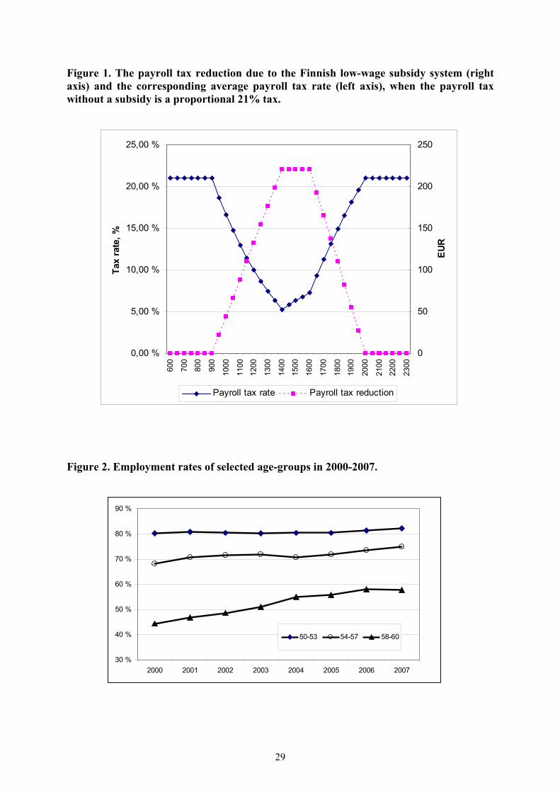
level of 2,000 €/month. Figure 1 illustrates the effects of the low-wage subsidy by plotting the

reduction in the payroll tax due to the system and the corresponding average payroll tax rate.

(Figure 1)

Finland has no minimum wage laws. However, union contracts also cover non-union workers

so that in practice the lowest legal wages are set in union contracts for about 95 per cent of the

workers. In union contracts, the lowest wages vary across sectors, regions and tasks. In typical

low-wage sector contracts, the lowest full-time wages were around 1,300 in 2006. (1,280

€/month in the retail trade, 1,301 €/month in hotels and restaurants and 1,249 €/month for

security guards). In comparison one could note that according to Statistics Finland the average

wage for full-time workers was around 2,500 euros in 2006. The subsidy is therefore targeted at

workers that are well below the average wage, with the maximum subsidy paid to those whose

wage is close to the minimum wage.

____________________ 7 Whether the system will be continued will depend on its effectiveness during the experimental period. Since the experiment will be quite long, it is reasonable to believe that firms can react to it and therefore the evaluation of this system will also reveal relevant information for a truly permanent scheme.

11

All employers except the national government are eligible for the low-wage subsidy. The

employer calculates the amount of subsidy itself and reduces the amount of its monthly tax

payments by the amount of the subsidy. In the January following the tax year the employer is

required to report the amounts that have been deducted, itemised by month and employee, to

the tax authorities.

An interesting feature of the subsidy system is that most full-time workers, especially those in

the age range eligible for the low-wage subsidy, earn more than 1,400€/month, which means

that the payroll tax is progressive for their employers. The effects of progressivity on wages

and employment crucially depend on whether the labour market is competitive or not. In

competitive labour markets, an increase in progressivity typically reduces labour supply,

whereas in an imperfect labour market, the opposite may hold. For example, in union models, a

revenue-neutral increase in tax progressivity can increase employment, since it renders nominal

wage increases less profitable for the unions, tilting the balance between employment and high

wages in favour of increased employment (see e.g. Lockwood and Manning 1993, Holmlund

and Kolm 1995 and Koskela and Vilmunen 1996). This is a relatively robust result that has

garnered some empirical support, and it also holds under different labour-market imperfections

(see e.g. the discussion in Sørensen 1997).

However, the mirror image of this result is that gross wages for low-paid workers may rise less

than they would have risen in the absence of the progressive payroll tax system.8 Second, even

if a rise in tax progressivity may increase employment at the extensive margin (i.e. the number

of employees), it can still reduce the hours of work or, more generally, effort by individual

workers at the intensive margin.9 Therefore, it is also important to account for how the hours

that are worked change because of the reform.

8 This is, in fact, what some unions, where a large proportion of members are in the low-wage area, feared and therefore they opposed the introduction of the low-wage subsidy system. 9 This point had already been examined by Jackman and Layard (1990). In the long term, tax progressivity can also reduce the incentives to acquire education.

12

4. EMPLOYMENT RATES BY AGE

As a first attempt to assess the employment effects of the wage subsidies we use data from the

Labour Force Survey. We do not have micro-data at our disposal but we used employment

rates and average hours per employed worker both calculated for one-year age groups. These

data are unpublished tables produced for internal use at Statistics Finland. Statistical

publications report similar numbers aggregated to five-year age groups.

We use data on employment rates and hours per employee for one-year age-groups between 50

and 60 from the period 2001 – 2007 and specify a simple fixed-effects model that captures

differences in employment rates across age groups and general trends in the labour markets.

The effect of the subsidy scheme is captured by an interaction term indicating that the subsidy

system has been implemented (year ≥ 2006) and that the age-group is eligible for the subsidy

(age ≥ 54). The equation to be estimated is therefore

itttiiitit yearDageDy εβα +Φ+Ω++= )()(SUBSIDY ,

where yit is the variable of interest i.e. the employment rate or average hours of age group i in

year t. The coefficient β is an unbiased estimate of eligibility for the subsidy if there are no

other age-specific trends that are correlated with the subsidy scheme. As can be seen from

Figure 2 this assumption is likely to be violated. Employment rates for the older age groups had

been increasing for several years before the introduction of wage subsidies for reasons clearly

unrelated to the subsidy scheme. To avoid interpreting these changes as an effect of wage

subsidies for workers over 54, we add age-specific linear trends to the equations that we

estimate.

(Figure 2)

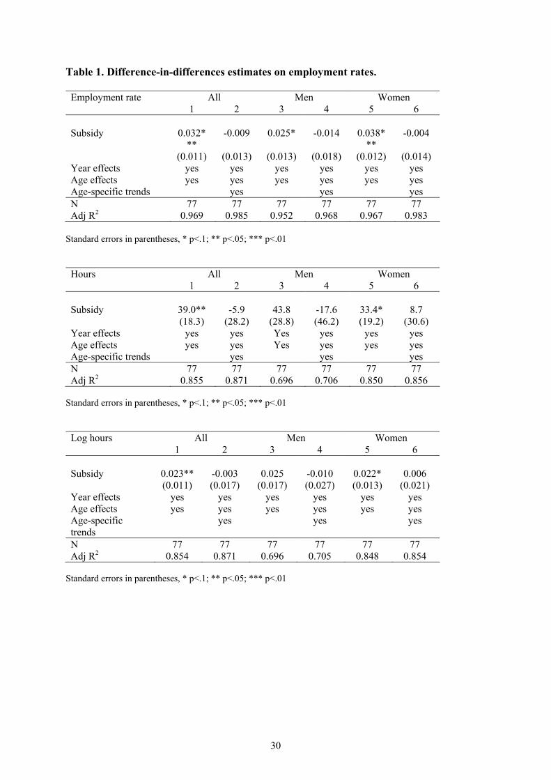
The results are displayed in Table 1. We first report the effect of the subsidy on employment

rates and then hours and per employee. The first two columns include both men and women.

The next columns report the results for men and women separately. All equations include a full

set of age and year dummies; coefficients of these dummy-variables are not reported in the

table.

13

The simple fixed-effects estimates reported in Columns 1, 3, and 5 indicate that the difference

in the employment rates before and after the introduction of the subsidy system is on average

3.2 per cent higher in the age groups eligible for the subsidy than in the younger age groups.

Also, hours per employed worker seem to have increased by 39 hours per year or by 2.3

percentage points. However, both these changes seem to be due to a general increase in

employment in the older age groups. After adding cohort-specific trends to the equations the

estimated effect decreases to close to zero and is not significant in any specification.

(Table 1)

If the employment rates of the older age groups had increased after the reform we should have

been able to detect them by using data from the Labour Force Survey. Focusing on the

employment rates instead of the number of employed workers also captures the changes in the

cohort size controlling for the changes in the labour supply. The drawback to the Labour Force

Survey is that information on wages is not available (and even information on education is

lacking from our data). Hence, we could not capture differential changes in low-wage and high-

wage employment. This is why we now proceed to our main analysis of DDD estimates, first in

Section 5, on entry (using register-data of the unemployed) and, second in Section 6, on exit

rates, hours of work and wage rates (using data from the employers’ organisation).

5. ENTRY OF THE UNEMPLOYED TO THE WORKFORCE

We analyse the effect of the subsidy on re-employment rates using individual-level data from

Finnish Longitudinal Census files. The data contains a 33% random sample of population that

resided in Finland at some point between 1990 and 2006 and hence also a random sample of

the unemployed at any given point in time. We take three separate cross-sections of data

containing those who were unemployed in the last week of the years 2003, 2004 and 2005 and

follow them up to the end of the following year. To focus on the elderly unemployed we limit

the data to those between the ages of 45 and 59 at the time when we draw the samples. The

unemployed in the first two cross-sections are not eligible for the subsidy but those who were

unemployed in the end of 2005 become eligible from the beginning of 2006 if they are over 54

years old in 2006. It would probably have been useful to include more post-reform years but

2006 was the latest available year in the database.

14

We therefore define the treatment group as those over 54 by the end of the following year and

leave the younger age groups in the control group. We then compare the changes in the re-

employment rates in these groups over time. Finding that the re-employment rates of the

treatment group increased in 2006 would provide evidence on the effects of the subsidy.

As wages for the unemployed are not available, we cannot create treatment and control groups

based on the wage level. As a partial solution we split the data by education into those with no

more than basic education and those with at least a secondary education; and by previous wage

into those whose pre-unemployment monthly wage was below 2,000 EUR and those whose

pre-unemployment wage was higher than that. Pre-unemployment wages are based on months

worked and annual income received during the previous year. To avoid excessive measurement

errors we only included data on those who had worked at least six months during the calendar

year. Since many unemployed workers have incomplete earnings histories we could calculate

reliable pre-unemployment wages for only about half of the sample.

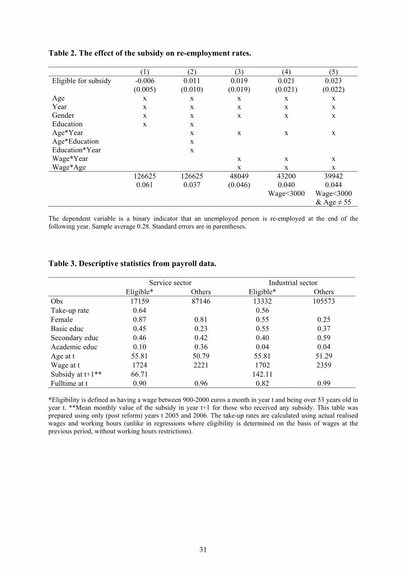
Table 2 presents the main results of the exercise. First, in Column 1 we report simple

difference-in-difference estimates where we control for the full set of age and year dummies

and define the treatment as an interaction of the post-reform period and an indicator that an

unemployed person will be over 54 by the end of the next year. The estimated effect turns out

to be close to zero and is not statistically significant. We also estimated the same model

separately for those with no more than basic education and for those with at least secondary

vocational education, but found no significant effects in either group. If those with no more

than basic education are more likely to be eligible for the subsidy, the interesting parameter is

the difference in the effect of the reform between groups differing in the level of education.

This is analysed in the second column that presents difference-in-difference-in-differences

estimates i.e. a coefficient of a triple interaction between the post-reform period, age over 54

and only compulsory education while controlling for the pair-wise interactions between these

variables. Now the coefficient is positive, indicating the re-employment rates of the

unemployed that are more likely to be eligible for the subsidy increase by one per cent due to

the reform. However, this estimate is not statistically significant either. In the third column we

use an indicator of previous wages that are below 2000 euros instead of an indicator of low

education. Due to missing wage data the sample size is dramatically reduced. The estimate is

larger than in the previous column but still insignificantly different from zero. In Column 4 we

limit the comparison group to those whose previous monthly wage is below 3000 euros and in

Column 5 exclude the unemployed who are 55 because their early retirement benefits changed

15

in 2005 in a way that is likely to increase re-employment incentives. Neither has much effect

on the estimates.

(Table 2)

6. THE IMPACT OF THE LOW-WAGE SUBSIDY ON JOB EXIT

RATES, WAGES AND WORKING HOURS

In this section we examine the impact of the low-wage subsidy scheme on the probability of

exiting from current employment. As entry into new jobs is relatively rare at old ages, reducing

exits could be a key channel to how the subsidy could affect employment. Focusing on exits is

also helpful, as the subsidy is based on a wage level which is not observed for those not

working. In addition, we examine the effect of the low-wage subsidy on wages and working

hours for those who remain in their current job.

6.1. Data

The data for this section come from the payroll records of the Finnish employers’ association.

The data cover all private sector workers in firms that are members of the association and

provide information about monthly wages, working time, and some information about workers’

individual characteristics such as age, gender and education. In addition, we have access to

register data from the tax authorities that includes the actual subsidies paid to all individuals in

Finland.

The firms that are members of the employers’ association send their wage data to the

employers’ association once a year. Data is at the individual level and covers all employees

except the firm’s top management. In the service sector the employers’ association collects data

each October. In the industrial sector the data refers to December for those receiving monthly

salaries and to the last quarter of the year for those receiving hourly wages.

The main benefit of the data is that wages are accurately reported. In most firms the wage data

comes directly from the firm’s pay system. Hours are also reported accurately in the firms that

16

pay hourly wages. The firms that pay monthly salaries typically only report normal weekly

hours. Even this information is likely to be more reliable than self-reported hours in household

surveys.

The data contains pseudo ID codes identifying each person and each firm that allow the same

person to be followed over time as long as the person remains employed by a firm that is

included in the data. Unfortunately, we have no information on what happens to persons if they

disappear from the data. They may have moved to the public sector, become unemployed or

retired. The firm identifiers can be used for calculating the number of employees in each firm

and for identifying employees that change firms.

6.2. Set up

The sample that we use in the empirical analysis is constructed as follows. We have two years

of data before the reform (2004 and 2005) and two years after the reform (2006 and 2007). We

drew four separate samples: for each year (t+1); we take those employed at the end of the

previous year (t) and follow them until the end of year t+1. To limit the comparison group to

reasonably similar workers we restricted both samples to those over 45 and below 59 years at

the time when the wage information was collected (time t). In addition, we only consider

employees whose wage is less than 3,000 € per month.

We determine eligibility for the subsidy based on age and monthly wage in year t, and calculate

the subsidy based on monthly wage in that year. We begin by dividing the data into two age

groups (below 54/above 54) and two wage groups (below 2,000/above 2,000). We thus have

four different age-wage categories. Our treatment group is the workers who are eligible for the

subsidy, i.e. older low-wage workers.

Notice that we do not restrict the treatment group to full-time workers. If we did this, we would

not capture the possibility that a part-time worker could become a full-time worker because of

the introduction of the subsidy.10

10 On the other hand, the treatment group now includes part-time workers who are not eligible for the subsidy. We also analysed the case where the treatment group was restricted to full-time workers. See the discussion at the end of Section 6.

17

Table 3 collects some descriptive analysis of the target and the control group in the post-

reform years, 2006 and 2007. Most eligible workers work in the service sector. The take-up

rate is calculated as the share of those who actually received the benefit in year t+1 according

to data from the Tax Register to those who would eligible for the benefit according to the wage

and the working hours reported in the employers’ association data. Analysis of the take-up rate

reveals that take-up is higher in bigger firms and in firms where the mean wage is smaller than

the average.11

The share of female workers in the treatment group is higher than their average share in both

sectors. Not surprisingly, workers in the treatment group are also less educated than other

workers. The mean wage in the eligible group is at the phase-out range of the subsidy,

suggesting that most of the target group employees face a progressive payroll tax system.

(Table 3)

The goal of this part of the study is to identify the effect of the low-wage subsidy on the

employment of the treatment group. Identifying this effect requires controlling for any

systematic shocks to the labour-market outcomes of the treatment group that are correlated with

but not due to the subsidy. We use difference-in-difference-in-differences strategies to

overcome these problems. This strategy can be described as follows. First, we include year

effects to capture any systematic overall trends in employment and earnings during the time the

subsidy was introduced. Second, we include a dummy for the treatment group (workers eligible

for the subsidy based on their earnings in year t and age) to control for permanent employment

and earnings differentials between the treatment group and other workers. Finally, we include

both age-by-year effects and wage group-by-year effects. That is, we compare the change in the

outcome for treatment individuals (older low-wage workers) with the change in the outcome

for control individuals within the same wage group (younger low-wage group), and compare

this with the difference in difference of outcome between older high-wage workers and

younger high-wage workers. This is the “difference-in-difference-in-differences” (DDD)

estimator. Its identifying assumption is that there is no contemporaneous shock that affects the

relative outcomes of the treatment group differently than other older workers or other low-wage

workers.

11 Representatives of the federations of industries and entrepreneurs have suggested that cumbersome

18

We begin by estimating the effect of the low-wage subsidy on the job exit rate. We defined

those who were not found in the same firm the next year (t+1) as leavers. The regression

equation has the following form:

)**()*()*()*()1|0(

876

543211

WAGEGAGEGYEARWAGEGYEARAGEGYEARWAGEGAGEGWAGEGAGEGYEAREEP

tittitt

ittttititit

ββββββββα

++++++++===+ X (1)

In this equation i indexes individuals, t indexes years, itX is a vector of individual

characteristics, )1|0( 1 ==+ itit EEP is the probability that a worker leaves a firm between t and

t+1. YEAR controls for common time shocks, AGEG is an age group dummy, which controls

for permanent differences between older and younger workers, WAGEG is a wage group

dummy, which controls for permanent differences between low wage and high wage workers,

AGEG*WAGEG controls for time-invariant characteristics of the treatment group,

YEAR*AGEG controls for the time-specific shocks that affect the outcome of older workers,

and YEAR*WAGEG captures the time-specific shocks common to low-wage workers. The

third level interaction term ( 8β ) captures all variations in outcome specific to older low-wage

workers after the introduction of the low-wage subsidy scheme.

We also estimate a specification where we replaced the treatment-dummy variable

)**( WAGEGAGEGYEARt with the amount of the subsidy the employer would be eligible

for. Now the effect of the subsidy is also identified from the differences in the size of the

subsidy among the eligible group. Since the size of the subsidy depends on the wage level we

replace the rough low-wage high-wage groups with finer 100 euro wage intervals. At the same

time we fully control for age by including it as one-year age dummies.

We calculated the low-wage subsidy that the firm would get for each worker in year t+1 if

his/her wage remained unchanged from year t. Since the payroll tax subsidy was introduced

only in 2006, this measure is zero for all workers in the 2003 and 2004 samples. For the 2005

sample the measure gets positive values if the 2005 wage is below 2,000 euros and if the

worker is over 53 (i.e. over 54 and hence eligible in 2006), and likewise for the 2006 sample.

Our model is therefore identified from the differences in the changes in job-leaving rates

between the group that becomes eligible for the low-wage subsidies and groups that are either

____________________ administrative details related to the subsidy system may explain why some firms have not applied for the subsidies.

19

too young to be eligible or have a wage exceeding 2,000 euros. In both cases we estimate the

impacts of eligibility for the low-wage subsidy, not the effect of actually receiving the subsidy.

As we report in the empirical section, the take-up rates were well below 100 per cent,

indicating that not all firms that are eligible for the subsidy ever apply for it12.

We then examine the effects on hours conditional on employment. In this analysis of

adjustment in the intensive margin we limit the data to those who are employed in the same

firm in both years t and t+1. We also examine the effects on hourly wages using data on the

workers who stay in the firm. The regression equation has the following form:

)**()*()*()*()log(

876

543211

WAGEGAGEGYEARWAGEGYEARAGEGYEARWAGEGAGEGWAGEGAGEGYEARY

tittitt

ittttitit

ββββββββα

++++++++=+ X

(2)

Where Y denotes the weekly working hours or monthly earnings in year t+1. We thus look at

the effect of subsidy eligibility on working hours and earnings.

6.3. Results

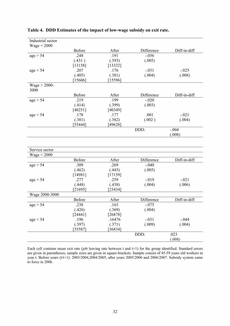
Table 4 illustrates a DDD estimation of the effect of low-wage subsidy on job-leaving rates for

the industrial sector. The upper panel compares the change in job exit rates for older low-wage

workers (treatment individuals) before and after the introduction of the low-wage subsidy

scheme with the change in the job exit rates of younger low-wage workers. Each cell contains

the mean job-leaving rate for the group labelled on the axes, along with standard errors and the

number of observations. There is a clear fall in the job-leaving rates for both groups during this

period. The difference-in-differences estimate, i.e. the difference in the changes of the job-

leaving rate between older and younger low-wage workers is -2.5 per cent. If there was a

distinct labour market shock that affected older workers over this period, this estimate would

not correctly identify the impact of the low-wage subsidy scheme. In the bottom panel we

perform the same exercise for high-wage workers. The difference between the change in the

job-leaving rate for older and younger high-wage workers is also negative, -2.1 per cent.

Taking the difference between these two panels, we get the DDD estimate, which is negative

but not statistically significant.

12 Our results should therefore be interpreted as effects of eligibility, or intention to treat effect.

20

In the lower panel we perform the same exercise for service sector workers. Now, while the

DD between older and younger low-wage workers indicates a 2.1 per cent fall in the job-

leaving rate, this difference is even more pronounced for high-wage workers (-4.4.). According

to the lower panel, the DDD estimate indicates that there was a 2% increase in the job-leaving

rate for older workers. The results in this table demonstrate the power and importance of the

DDD estimation. Without the other control group, one would mistakenly conclude that the

subsidy system was effective in reducing exit rates.

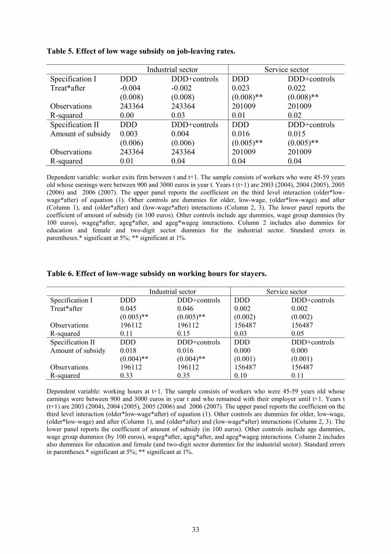
The first row of Table 5 presents the results of the same analysis in a regression framework.

We first re-report the coefficient of the treatment variable (older*low-wage*after) in our DDD

specification for industrial sector workers. We estimate this linear probability model by OLS.

In Column 2 we control for other observables, such as educational category (4), gender, union

contract, and two-digit industry. Adding these control variables does not render the coefficient

significant.

The lower panel reports the results of a specification where we explain the job-leaving rate by

the amount of the subsidy the worker’s employer is eligible for (in 100 euros). The

specification in the first column includes controls for age-group, wage-group and time period.

In the next column we report the results for a specification which controls for time-specific

shocks to age- and wage-groups, as well as age-group wage-group interaction. Now we find

that even if we take into account the actual amount of the subsidy the employers could be

eligible for, the system is still not effective in reducing exit rates. The result remains when

controls for gender, education and industry are included.

Columns 3 and 4 report the same estimations for service-sector workers. As illustrated in Table

4 according to the DDD specification there seems to be an approximately 2 per cent increase in

the job-leaving rate for those service-sector workers who are eligible for the subsidy. The

additional control variables include dummies for gender, educational category and educational

field. The results in the lower panel indicate a 1.5 % increase in exit probability. These results

are clearly puzzling. It should be noted, however, that this does not necessarily indicate a

higher exit to non-employment, since leavers may also be moving to another job.

Since some of the workers were also affected by the pension reform, we have checked the

robustness of the results when those who were 55 years old at time t (the group whose early

21

retirement channel changed) are dropped from the sample. The qualitative results remain the

same: the exit rates did not decline in a statistically significant way in either sector.13

Next, we analyse how low-wage subsidies affected working hours and earnings for those who

remained with their employer. Table 6 reports the OLS estimates of the third-level interaction

from equation (1), where the dependent variable is now the log weekly working hours. From

the upper panel, we find that the introduction of the wage subsidy increased the working hours

for older workers in the industrial sector by almost 4.5 per cent. The lower panel suggests,

however, that when measured by the actual amount of the subsidy the employers are eligible

for, the impact on working hours decreases to 1.8 per cent. There are probably some non-linear

effects on working hours, depending on the workers’ wage level. There seems to be no effect of

the low-wage subsidy for service-sector workers. We also looked to see whether this increase

in working hours was due to a possible increase in the share of full-time workers within the

group of older low-wage workers. Our results (not reported) indicated that the low-wage

subsidy did, in fact, significantly increase the likelihood of becoming a full-time worker for

part-time workers in the industrial sector14.

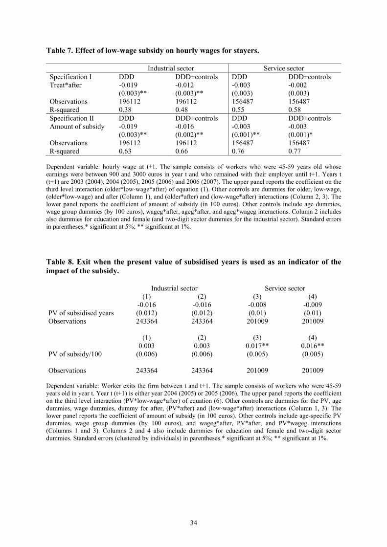
Table 7 reports the results of regression where the dependent variable is log real hourly wages.

The sample consists of stayers, i.e. workers who have remained with the same employer for at

least two periods. For the industrial sector there seems to be an almost 2 per cent decrease in

hourly wages. For the service sector the results are less clear. The low wage subsidy had no or

very little effect on hourly wages15.

All these estimations were carried out using the subsidy eligibility definition, which is based on

age and earnings in year t. This includes both part-time and full-time workers. As a robustness

check we examined how results change if eligibility for the subsidy is restricted only to full-

time workers in year t. We included controls for full-time work in time t in these regressions.

This did not have an effect on our results.

13 These results are available from the authors upon request. 14 The subsidy increased the likelihood of becoming a full-time worker by 7 per cent. Subsidies had no impact on the working hours of workers who were already full-time workers in year t. 15 Even though the hourly wages decreased in the industrial sector, the monthly wages increased, since there was an overall increase in working hours.

22

7. SOME EXTENSIONS

7.1. Taking ageing into account

The analysis above is based on a sharp distinction between the treatment group and the control

group. This does not take into account the possibility that, because of the subsidy system, an

employer may want to keep a low-wage worker who is 53 because he will soon be eligible for

the subsidy. Therefore, the subsidy can also have positive externalities for people outside the

treatment group through anticipation effects.16

We will take into account these considerations as follows. We first calculate age-specific

retention rates based on pre-reform data. Then, for example, the probability that a 52-year-old

worker will stay in the same firm until he or she is eligible for the subsidy is

54,5353,5254,52 * ppp = , where jip , denotes the probability of a worker of i years of age staying

in the firm until he is j years old, conditional on his having been in the firm when he was i years

old. Now the key explanatory variable is the expected number of subsidized years that is also

positive for workers younger than 54.

Then we use this notion, which we call the present value of the subsidy (PV), in place of the

‘AGEG’ (age group) terms in the regressions as below:

)**()*()*()*()1|0(

,876

543211

titittitt

ittttititit

PVWAGEGYEARPVYEARPVYEARWAGEGPVWAGEGPVYEAREEP

ββββββββα

++++++++===+ X , (6)

which is otherwise similar to the earlier exit regression (1), but the variable AGEG is replaced

by the age-specific present values of subsidised years (the PVs). Again, the interesting variable

is the last, triple interaction, term.

The results for the exit rate, presented in Table 8, that take into account the correction for

ageing are in line with earlier results presented in Table 4: the subsidy system did not reduce

the exit rates in a statistically significant way.

16 Another kind of anticipation effect would arise if the subsidy system were foreseen in years before the system took effect. However, the system was introduced so late (in budget negotiations in early autumn 2005; the corresponding legislation was passed even later) that this complication is likely to play a very small role.

23

7.2. Take-up

As noted above, the comparison of changes in the exit rates, hours worked and wages between

those who are eligible for the low-wage subsidy and those who are not reveals the impact of the

reform, not the impact of actually receiving wage subsidies. As long as we are primarily

concerned about the effects of introducing a low-wage subsidy policy, this is probably the main

parameter of interest. However, incomplete take-up is likely to lead to smaller employment

effects than a policy that would automatically reduce payroll taxes for the eligible workers. If

we are interested in evaluating the effects of actually receiving low-wage subsidies or in

identifying labour demand elasticities due to a reduction in the labour costs, we need to account

for the incomplete take-up rates.

Moving away from analysing the effects of the policy change to the effects of a reduction in

payroll taxes immediately introduces serious selectivity problems. While we can probably treat

the change in policy as an exogenous effect from the perspective of the firm, we cannot ignore

the fact that those firms that actually apply for the wage subsidies are not a randomly selected

sub-group of eligible firms.

A standard solution to this selectivity problem is to use eligibility for subsidies as an instrument

for receiving subsidies. A simple model (omitting the year, age and wage dummies for

simplicity) consists of a two-equation system

iii

iii

RSSY

νλκεβα

++=++=

(7)

where Y is the outcome of interest, S indicates that the firm receives subsidies (or the amount of

subsidy) for the worker i, and R that the firm is eligible for the subsidies (or the amount that the

firm is entitled to). In the simplest case, where both equations are linear and both the eligibility

for the subsidy and recipiency of the subsidy are dummy variables, the IV estimate for the

effect of the subsidy is the Wald estimate

]0|[]1|[]0|[]1|[

=−==−=

=iiii

iiiiWALD RSERSE

RYERYEβ (8)

24

The numerator in this expression is the difference in the outcome variable between the persons

that are eligible for the subsidy, and the denominator is the difference in the fraction actually

receiving the subsidy. If receiving the subsidy is impossible for those who are not eligible for

the subsidy 0]0|[ ==ii RSE , the Wald estimate simply scales up the effects by multiplying

the difference between eligible and ineligible persons by the inverse of the take-up rate. One

should also note that as long as eligibility for the subsidy has some effect on the fraction

receiving subsidies the denominator of the equation is strictly positive, and inferences on

whether the effect is significantly different from zero can be based directly on the numerator.

Hence, if eligibility for the subsidy has no significant effect on the outcome of interest, neither

has actually receiving the subsidy had any effect.

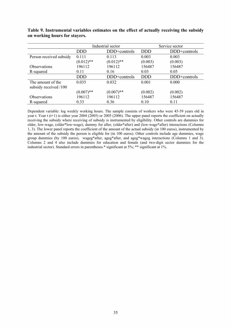
To illustrate the role of the take-up rate, we show the impact of actually receiving the subsidy

on working hours when eligibility for the subsidy is used as an instrument for received

subsidies (Table 9). As expected, the point estimate of the subsidy has increased in the

industrial sector: since the take-up rate is close to 50%, the coefficient of the actual subsidy is

roughly two times larger than the coefficient of eligibility alone. In the service sector, since the

effects of eligibility are not significant, neither are the impacts of actually receiving the

subsidy. The results regarding earnings (not shown) follow the same pattern.

7.3. Other potential extensions

The usual worry with the targeted subsidy systems is whether they lead to substitution or

replacement effects. This ‘revolving door’ issue may arise if employers simply shed ineligible

workers to be able to benefit more from the subsidies for eligible workers. Then even if the

share of the targeted workers rises, overall employment may not necessarily increase. Given

that we did not find statistically significant employment effects for the target group, there is

little need to examine the substitution effects in our case.

Finally, if the goods market is non-competitive, the tax cut may also lead to increased profits

because the market prices of the final goods do not necessarily move in a one-to-one relation

with marginal costs. (See the analysis in e.g. Myles, Ch. 11, (1995) for commodity taxes; the

analytics are similar with respect to the taxation on labour.) Preliminary analysis using data on

Finnish corporations, combined with information about firm-specific low-wage subsidies, does

25

not seem to reveal robust linkages between the amount of subsidies received and the profit

rates.17

8. CONCLUSIONS

While low-wage subsidies are often regarded as a promising way to improve the labour-market

prospects of low-skilled workers, the current evidence on their effectiveness is scarce. The

evidence is mainly based on universal subsidy schemes that are difficult to evaluate because of

the lack of a natural comparison group. Using detailed, individual-level, panel data, this paper

estimated the employment effects of a Finnish low-wage subsidy scheme that was targeted to

low-wage older workers. The clear eligibility criteria opened up a way to use the DDD

estimation strategy that allows for controlling for, for example, time-varying differences for

labour demand of a given skill category. In fact, we find that leaving out the other control

group, essentially returning to the standard DiD analysis similar to earlier papers in the field,

would produce upwards-biased estimates of the impacts of the subsidy system.

The results indicate that the subsidy scheme was not effective in increasing the employment of

eligible workers. However, it might have led to increased working hours in the industrial sector

by making some former part-time workers work full-time. The results regarding the impacts on

wages are somewhat ambiguous: monthly wages rise, but hourly wages (in comparison to

wages in the control groups) seem to have dropped in some cases. This is interesting because it

is, in fact, one of the theoretical predictions of the impacts of progressive taxes under

imperfectly competitive labour markets.

We also considered a number of extensions to the basic analysis, including the fact that

workers close to the eligible age are ‘almost’ in the treatment group if they stay in the same

firm, and imperfect take-up rates. These extensions did not change the basic qualitative results

above.

17 This issue was analysed using register-data of all Finnish corporations, available from the tax authorities, from 2004-2007. The profit rate (profit/turnover) was explained in a fixed-effects framework by the subsidy (divided by turnover) the firm received and firm and year dummies. This analysis did not provide evidence that subsidies had increased the profitability of the subset of firms that received them.

26

Quite why the results are so disappointing remains unclear. Perhaps the subsidy has not been

sufficiently large, given that the treatment group (elderly workers) can consist of workers for

whom it is particularly difficult to remain employed or to be hired. Or perhaps the wage

demand for these workers is simply inelastic. Needless to say, these results cannot be regarded

as a universal case against low-wage subsidies. What they demonstrate is the need for careful

evaluation of these schemes that can, one hopes, in the end, help design the schemes in the best

possible way.

References:

Adda, J., Costa Dias, M., Meghir, C., Sianesi, B. (2007): Labour Market Programmes and

Labour Market Outcomes: A Study of the Swedish Active Labour Market Interventions,

mimeo.

Bell, B., R. Blundell and J. Van Reenen (1999) ‘Getting the Unemployed Back to Work: The

Role of Targeted Wage Subsidies’, International Tax and Public Finance, 6, 339-360.

Bennmarker, H., E. Mellander, and B. Öckert (2009) ‘Do regional payroll tax reductions

boost employment?’ Labour Economics (forthcoming).

Blundell, R. (2006) ‘Earned Income Tax Credit Policies: Impact and Optimality, The Adam

Smith Lecture 2005’, Labour Economics 13, 423-443.

Bovenberg, A. Lans & Graafland, Johan J. & de Mooij, Ruud A. (2000) ‘Tax reform and the

Dutch labor market: an applied general equilibrium approach’, Journal of Public Economics

78, 193-214.

Brown, A., C. Merkl and D. Snower (2007) ‘Comparing the effectiveness of low-wage

subsidies’, CEPR Discussion Paper No. 6334.

Calmfors, L.; A. Forslund and M. Hemström (2004) ‘The effects of active labour market

policies in Sweden: What is the evidence?’, in J. Agell, M. Keen and A.J. Weichenrieder

(Eds.) Labor Market Institutions and Public Regulation, MIT Press.

Card, D. and D. Hyslop (2005) ‘Estimating the Effects of a Time-Limited Earnings Subsidy

for Welfare Leavers’ Econometrica, 73 (6), 1723–1770.

Chéron, A., J.-O. Hairault and F. Langot, (2008) ’A quantitative evaluation of payroll tax

subsidies for low-wage workers: An equilibrium search framework’, Journal of Public

Economics 92, 817-843.

27

Crépon B. and R. Desplatz (2002) ‘Evaluating the effects of payroll tax subsidies for low

wage workers’, INSEE mimeo.

Drèze, J.H. and E. Malinvaud (1994) ‘Growth and Employment: The Scope for a European

Initiative’, European Economy, No. 1. 77–106.

Edlin, A. and E. Phelps (2009) ‘Getting serious about job creation: Part I’, The Economists’

Voice 6, Issue 5, Article 3.

Eissa, N. and H. Hoynes (2004) ’Taxes and the labor market participation of married couples:

the earned income tax credit’, Journal of Public Economics 88, 1931–1958.

Eissa, N. and J. Liebman (1996) ’Labor supply response to the earned income tax credit’

Quarterly Journal of Economics CXI, 605–637.

Gesine, S. (2009) Employer wage subsidies and wages in Germany. IAB Discussion Paper

9/2009.

Goos, M. and J. Konings (2007), ‘The Impact of Payroll Tax Reductions on Employment and

Wages: A Natural Experiment Using Firm Level Data,’ LICOS Discussion Papers 17807.

Gruber J (1994) “The Incidence of Mandated Maternity Benefits” American Economic

Review 84(3), 622–641.

Holmlund, B. and A.-S. Kolm (1995) ‘Progressive Taxation, Wage Setting, and

Unemployment: Theory and Swedish Evidence. Swedish Economic Policy Review 2, 423-

460.

Jackman, R. and R. Layard (1990) ‘The Real Effects of Tax-based Incomes Policies’,

Scandinavian Journal of Economics 92, 309-324.

Katz, L. (1996) ‘Wage subsidies for the disadvantaged’ NBER Working Paper 5679.

Knabe, A. and R. Schöb (2008) ‘Minimum wages and their alternatives: A critical

assessment’, CESifo Working Paper No. 2494.

Knabe, A., R. Schöb and J. Weimann (2006) ‘Marginal employment subsidization: A new

concept and a reappraisal’, Kyklos 59, 557-577.

Korkeamäki, O. and R. Uusitalo (2009) ‘Employment and wage effects of a payroll-tax cut:

Evidence from a regional experiment’, International Tax and Public Finance, forthcoming.

Koskela, E. and J. Vilmunen (1996) ‘Tax Progression is Good for Employment in Popular

Models of Trade Union Behaviour’, Labour Economics 3, 65-80.

28

Kramarz, F. and T. Philippon (2001) ‘The impact of differential payroll tax subsidies on

minimum wage employment’, Journal of Public Economics 82, 115-146.

Lockwood B and Manning A. (1993) Wage setting and the tax system. Theory and evidence

for the United Kingdom. Journal of Public Economics 52:1–29.

Michalopoulos, C., D. Tattrie, C. Miller, P. Robins, P. Morris, D. Gyarmati, C. Redcross, K.

Foley, R. Ford (2002) ‘Making Work Pay: Final Report of the Self Sufficiency Project for

Long Term Welfare Recipients’. Ottawa: Social Research and Demonstration Corporation.

Myles, G. (1995) Public Economics. Cambridge University Press.

Phelps, E. (1994) “Low-Wage Employment Subsidies versus the Welfare State”, American

Economic Review, Papers and Proceedings ,84, 54-58.

Phelps, E. (1997) Rewarding Work: How to Restore Participation and Self-Support to Free

Enterprise, Cambridge, MA: Harvard University Press.

Sianesi, B. (2008): Differential Effects of Active Labour Market Programs for the

Unemployed, Labour Economics 15, 392-421.

Sørensen, P.B. (1997) ‘Public Finance Solutions to the European Unemployment Problem?’

Economic Policy October 1997, 223-264.

29

0,00 %

5,00 %

10,00 %

15,00 %

20,00 %

25,00 %

600

700

800

900

1000

1100

1200

1300

1400

1500

1600

1700

1800

1900

2000

2100

2200

2300

Tax

rate

, %

0

50

100

150

200

250

EUR

Payroll tax rate Payroll tax reduction

30 %

40 %

50 %

60 %

70 %

80 %

90 %

2000 2001 2002 2003 2004 2005 2006 2007

50-53 54-57 58-60

Figure 1. The payroll tax reduction due to the Finnish low-wage subsidy system (right axis) and the corresponding average payroll tax rate (left axis), when the payroll tax without a subsidy is a proportional 21% tax.

Figure 2. Employment rates of selected age-groups in 2000-2007.

30

Table 1. Difference-in-differences estimates on employment rates. Employment rate All Men Women 1 2 3 4 5 6 Subsidy 0.032*

** -0.009 0.025* -0.014 0.038*

** -0.004

(0.011) (0.013) (0.013) (0.018) (0.012) (0.014) Year effects yes yes yes yes yes yes Age effects yes yes yes yes yes yes Age-specific trends yes yes yes N 77 77 77 77 77 77 Adj R2 0.969 0.985 0.952 0.968 0.967 0.983

Standard errors in parentheses, * p<.1; ** p<.05; *** p<.01 Hours All Men Women 1 2 3 4 5 6 Subsidy 39.0** -5.9 43.8 -17.6 33.4* 8.7 (18.3) (28.2) (28.8) (46.2) (19.2) (30.6) Year effects yes yes Yes yes yes yes Age effects yes yes Yes yes yes yes Age-specific trends yes yes yes N 77 77 77 77 77 77 Adj R2 0.855 0.871 0.696 0.706 0.850 0.856

Standard errors in parentheses, * p<.1; ** p<.05; *** p<.01 Log hours All Men Women 1 2 3 4 5 6 Subsidy 0.023** -0.003 0.025 -0.010 0.022* 0.006 (0.011) (0.017) (0.017) (0.027) (0.013) (0.021) Year effects yes yes yes yes yes yes Age effects yes yes yes yes yes yes Age-specific trends

yes yes yes

N 77 77 77 77 77 77 Adj R2 0.854 0.871 0.696 0.705 0.848 0.854

Standard errors in parentheses, * p<.1; ** p<.05; *** p<.01

31

Table 2. The effect of the subsidy on re-employment rates. (1) (2) (3) (4) (5) Eligible for subsidy -0.006

(0.005) 0.011

(0.010) 0.019

(0.019) 0.021

(0.021) 0.023

(0.022) Age x x x x x Year x x x x x Gender x x x x x Education x x Age*Year x x x x Age*Education x Education*Year x Wage*Year x x x Wage*Age x x x 126625 126625 48049 43200 39942 0.061 0.037 (0.046) 0.040 0.044 Wage<3000 Wage<3000

& Age ≠ 55 The dependent variable is a binary indicator that an unemployed person is re-employed at the end of the following year. Sample average 0.28. Standard errors are in parentheses. Table 3. Descriptive statistics from payroll data. Service sector Industrial sector Eligible* Others Eligible* Others Obs 17159 87146 13332 105573 Take-up rate 0.64 0.56 Female 0.87 0.81 0.55 0.25 Basic educ 0.45 0.23 0.55 0.37 Secondary educ 0.46 0.42 0.40 0.59 Academic educ 0.10 0.36 0.04 0.04 Age at t 55.81 50.79 55.81 51.29 Wage at t 1724 2221 1702 2359 Subsidy at t+1** 66.71 142.11 Fulltime at t 0.90 0.96 0.82 0.99

*Eligibility is defined as having a wage between 900-2000 euros a month in year t and being over 53 years old in year t. **Mean monthly value of the subsidy in year t+1 for those who received any subsidy. This table was prepared using only (post reform) years t 2005 and 2006. The take-up rates are calculated using actual realised wages and working hours (unlike in regressions where eligibility is determined on the basis of wages at the previous period, without working hours restrictions).

32

Table 4. DDD Estimates of the impact of low-wage subsidy on exit rate. Industrial sector Wage < 2000 Before After Difference Diff-in-diff age > 54 .248

(.431 ) [13158]

.191 (.393)

[13332]

-.056 (.005)

age < 54 .207 (.405)

[15606]

.176 (.381)

[15596]

-.031 (.004)

-.025 (.008)

Wage > 2000-3000

Before After Difference Diff-in-diff age > 54 .219

(.414) [40251]

.199 (.399)

[40349]

-.020 (.003)

age < 54 .178 (.381)

[55444]

.177 (.382)

[49628]

.001 (.002 )

-.021 (.004)

DDD: -.004 (.008)

Service sector Wage < 2000 Before After Difference Diff-in-diff age > 54 .309

(.462) [14981]

.269 (.443)

[17159]

-.040 (.005)

age < 54 .277 (.448)

[21695]

.259 (.438)

[23434]

-.019 (.004)

-.021 (.006)

Wage 2000-3000 Before After Difference Diff-in-diff age > 54 .238

(.426) [24441]

.163 (.369)

[26878]

-.075 (.004)

age < 54 .196 (.397)

[35587]

.16476 (.371)

[36834]

-.031 (.009)

-.044 (.004)

DDD: .023

(.008) Each cell contains mean exit rate (job leaving rate between t and t+1) for the group identified. Standard errors are given in parentheses; sample sizes are given in square brackets. Sample consist of 45-59 years old workers in year t. Before years (t/t+1): 2003/2004,2004/2005, after years 2005/2006 and 2006/2007. Subsidy system came to force in 2006.

33

Table 5. Effect of low wage subsidy on job-leaving rates. Industrial sector Service sector Specification I DDD DDD+controls DDD DDD+controls Treat*after -0.004 -0.002 0.023 0.022 (0.008) (0.008) (0.008)** (0.008)** Observations 243364 243364 201009 201009 R-squared 0.00 0.03 0.01 0.02 Specification II DDD DDD+controls DDD DDD+controls Amount of subsidy 0.003 0.004 0.016 0.015 (0.006) (0.006) (0.005)** (0.005)** Observations 243364 243364 201009 201009 R-squared 0.01 0.04 0.04 0.04

Dependent variable: worker exits firm between t and t+1. The sample consists of workers who were 45-59 years old whose earnings were between 900 and 3000 euros in year t. Years t (t+1) are 2003 (2004), 2004 (2005), 2005 (2006) and 2006 (2007). The upper panel reports the coefficient on the third level interaction (older*low-wage*after) of equation (1). Other controls are dummies for older, low-wage, (older*low-wage) and after (Column 1), and (older*after) and (low-wage*after) interactions (Column 2, 3). The lower panel reports the coefficient of amount of subsidy (in 100 euros). Other controls include age dummies, wage group dummies (by 100 euros), wageg*after, ageg*after, and ageg*wageg interactions. Column 2 includes also dummies for education and female and two-digit sector dummies for the industrial sector. Standard errors in parentheses.* significant at 5%; ** significant at 1%. Table 6. Effect of low-wage subsidy on working hours for stayers. Industrial sector Service sector Specification I DDD DDD+controls DDD DDD+controls Treat*after 0.045 0.046 0.002 0.002 (0.005)** (0.005)** (0.002) (0.002) Observations 196112 196112 156487 156487 R-squared 0.11 0.15 0.03 0.05 Specification II DDD DDD+controls DDD DDD+controls Amount of subsidy 0.018 0.016 0.000 0.000 (0.004)** (0.004)** (0.001) (0.001) Observations 196112 196112 156487 156487 R-squared 0.33 0.35 0.10 0.11

Dependent variable: working hours at t+1. The sample consists of workers who were 45-59 years old whose earnings were between 900 and 3000 euros in year t and who remained with their employer until t+1. Years t (t+1) are 2003 (2004), 2004 (2005), 2005 (2006) and 2006 (2007). The upper panel reports the coefficient on the third level interaction (older*low-wage*after) of equation (1). Other controls are dummies for older, low-wage, (older*low-wage) and after (Column 1), and (older*after) and (low-wage*after) interactions (Column 2, 3). The lower panel reports the coefficient of amount of subsidy (in 100 euros). Other controls include age dummies, wage group dummies (by 100 euros), wageg*after, ageg*after, and ageg*wageg interactions. Column 2 includes also dummies for education and female (and two-digit sector dummies for the industrial sector). Standard errors in parentheses.* significant at 5%; ** significant at 1%.

34

Table 7. Effect of low-wage subsidy on hourly wages for stayers. Industrial sector Service sector Specification I DDD DDD+controls DDD DDD+controls Treat*after -0.019 -0.012 -0.003 -0.002 (0.003)** (0.003)** (0.003) (0.003) Observations 196112 196112 156487 156487 R-squared 0.38 0.48 0.55 0.58 Specification II DDD DDD+controls DDD DDD+controls Amount of subsidy -0.019 -0.016 -0.003 -0.003 (0.003)** (0.002)** (0.001)** (0.001)* Observations 196112 196112 156487 156487 R-squared 0.63 0.66 0.76 0.77

Dependent variable: hourly wage at t+1. The sample consists of workers who were 45-59 years old whose earnings were between 900 and 3000 euros in year t and who remained with their employer until t+1. Years t (t+1) are 2003 (2004), 2004 (2005), 2005 (2006) and 2006 (2007). The upper panel reports the coefficient on the third level interaction (older*low-wage*after) of equation (1). Other controls are dummies for older, low-wage, (older*low-wage) and after (Column 1), and (older*after) and (low-wage*after) interactions (Column 2, 3). The lower panel reports the coefficient of amount of subsidy (in 100 euros). Other controls include age dummies, wage group dummies (by 100 euros), wageg*after, ageg*after, and ageg*wageg interactions. Column 2 includes also dummies for education and female (and two-digit sector dummies for the industrial sector). Standard errors in parentheses.* significant at 5%; ** significant at 1%. Table 8. Exit when the present value of subsidised years is used as an indicator of the impact of the subsidy. Industrial sector Service sector (1) (2) (3) (4)

PV of subsidised years -0.016 (0.012)

-0.016 (0.012)

-0.008 (0.01)

-0.009 (0.01)

Observations 243364 243364 201009 201009 (1) (2) (3) (4)

PV of subsidy/100 0.003

(0.006) 0.003

(0.006) 0.017** (0.005)

0.016** (0.005)

Observations 243364 243364 201009 201009

Dependent variable: Worker exits the firm between t and t+1. The sample consists of workers who were 45-59 years old in year t. Year t (t+1) is either year 2004 (2005) or 2005 (2006). The upper panel reports the coefficient on the third level interaction (PV*low-wage*after) of equation (6). Other controls are dummies for the PV, age dummies, wage dummies, dummy for after, (PV*after) and (low-wage*after) interactions (Column 1, 3). The lower panel reports the coefficient of amount of subsidy (in 100 euros). Other controls include age-specific PV dummies, wage group dummies (by 100 euros), and wageg*after, PV*after, and PV*wageg interactions (Columns 1 and 3). Columns 2 and 4 also include dummies for education and female and two-digit sector dummies. Standard errors (clustered by individuals) in parentheses.* significant at 5%; ** significant at 1%.

35

Table 9. Instrumental variables estimates on the effect of actually receiving the subsidy on working hours for stayers. Industrial sector Service sector DDD DDD+controls DDD DDD+controls Person received subsidy 0.111 0.113 0.003 0.003 (0.012)** (0.012)** (0.003) (0.003) Observations 196112 196112 156487 156487 R-squared 0.11 0.16 0.03 0.05 DDD DDD+controls DDD DDD+controls The amount of the subsidy received /100

0.035 0.032 0.001 0.000

(0.007)** (0.007)** (0.002) (0.002) Observations 196112 196112 156487 156487 R-squared 0.33 0.36 0.10 0.11

Dependent variable: log weekly working hours. The sample consists of workers who were 45-59 years old in year t. Year t (t+1) is either year 2004 (2005) or 2005 (2006). The upper panel reports the coefficient on actually receiving the subsidy where receiving of subsidy is instrumented by eligibility. Other controls are dummies for older, low-wage, (older*low-wage), dummy for after, (older*after) and (low-wage*after) interactions (Columns 1, 3). The lower panel reports the coefficient of the amount of the actual subsidy (in 100 euros), instrumented by the amount of the subsidy the person is eligible for (in 100 euros). Other controls include age dummies, wage group dummies (by 100 euros), wageg*after, ageg*after, and ageg*wageg interactions (Columns 1 and 3). Columns 2 and 4 also include dummies for education and female (and two-digit sector dummies for the industrial sector). Standard errors in parentheses.* significant at 5%; ** significant at 1%.